# Bootstrap: the pymrm this page was checked with, and the gallery files it was
# published with. Works in a checkout, in CI and on a fresh Colab VM.
GALLERY_REF = "gallery-2026.11.10.3"  # replaced by the release tag at publication
PYMRM = ">=3.3.0,<4"  # equals meta.yaml pymrm_min_version, up to the next major
PAGE = "A2.3-taylor-aris-dispersion"  # equals the page directory

import os, sys, urllib.request
from pathlib import Path
_shared = next((p / "shared" for p in (Path.cwd(), *Path.cwd().parents)
                if (p / "shared" / "gallery_bootstrap.py").is_file()), None)
if _shared is None:
    _shared = (Path(os.environ.get("XDG_CACHE_HOME") or Path.home() / ".cache")
               / "pymrm-gallery" / GALLERY_REF)
    _shared.mkdir(parents=True, exist_ok=True)
    urllib.request.urlretrieve(
        "https://raw.githubusercontent.com/computational-chemical-engineering/"
        f"pymrm-gallery/{GALLERY_REF}/shared/gallery_bootstrap.py",
        _shared / "gallery_bootstrap.py")
sys.path.insert(0, str(_shared))
sys.modules.pop("gallery_bootstrap", None)
from gallery_bootstrap import setup
setup(PAGE, PYMRM, GALLERY_REF); # the semicolon stops the cell echoing the pathTaylor–Aris dispersion: how a velocity profile becomes a diffusivity
sec:A
struct:S3
struct:S6
tier:T0
data:tier2
phase:liquid
Shear plus molecular diffusion produces spreading that looks exactly like diffusion but is thousands of times faster. Solved two independent ways, checked against Taylor’s own capillary measurement, and the time it takes for his result to hold measured and derived.
Taylor–Aris dispersion: how a velocity profile becomes a diffusivity
Catalog ID: A2.3 · Structures: S3 (1-D steady BVP), S6 (2-D PDE) · Tier: T0
Push a slug of dye through a narrow tube in laminar flow and it spreads far faster than molecular diffusion could manage, yet it spreads symmetrically, as if by diffusion, despite a velocity profile that is anything but symmetric. Taylor explained why in 1953, and turned the effect into a way of measuring molecular diffusivities. This page computes his dispersion coefficient by two independent routes, recomputes his capillary measurement, and answers the question his paper leaves as an inequality: how long the slug must travel before his result holds.
import numpy as np
import matplotlib.pyplot as plt
from scipy.integrate import quad
from scipy.optimize import brentq
from scipy.special import j0, jn_zeros
from gallery_utils import load_data, load_meta, cite_data, Claims
from model import (closure, run_history, velocity_deviation, radial_grid,   # this page's model.py
                   radial_eigenvalue, Slug)

plt.rcParams.update({"figure.dpi": 110, "axes.grid": True, "grid.alpha": 0.3})
claims = Claims(PAGE.split("-")[0])
Background
In Poiseuille flow the fluid at the axis moves at twice the mean speed and the fluid at the wall does not move at all. A slug of solute released across the section should therefore be drawn out into a parabolic spike, sharply skewed, with a long tail at the axis.
That is not what happens. Taylor observed that after a while the slug is symmetric about a point moving at the mean speed, and spreads as though obeying Fick’s law with an effective diffusivity far larger than the molecular one. His explanation is a competition:
- shear stretches the solute axially, creating radial concentration gradients;
- molecular diffusion erases those radial gradients.
If the second is fast compared with the first, no radial gradient survives long enough to matter, the skew never develops, and what is left is symmetric spreading. The counter-intuitive consequence is that the dispersion coefficient is inversely proportional to the molecular diffusivity: making the solute diffuse faster radially makes the slug spread less axially, because it spends less time sampling the fast and slow streamlines separately.
This is the ancestor of every axial-dispersion coefficient in reactor modelling, and it is why an S4 breakthrough curve can use a single lumped \(D_{\mathrm{ax}}\) instead of resolving the radial profile.
The published model
The full problem (Taylor’s Eq. 11) is a 2-D axisymmetric advection-diffusion in a tube of radius \(a\) with Poiseuille flow:
\[ \frac{\partial C}{\partial t} + u(r)\frac{\partial C}{\partial x} = D\left[\frac{1}{r}\frac{\partial}{\partial r}\!\left(r\frac{\partial C}{\partial r}\right) + \frac{\partial^2 C}{\partial x^2}\right], \qquad u(r) = u_0\left(1 - \frac{r^2}{a^2}\right), \]
with \(\partial C/\partial r = 0\) at the axis and the wall. \(u_0\) is the centreline velocity; the cross-sectional mean is \(u_0/2\).
Taylor’s result (his Eq. 25). Relative to a plane moving at \(u_0/2\), the section-mean concentration disperses as if by diffusion with
\[ k = \frac{a^{2} u_0^{2}}{192\, D}. \]
Written with the mean velocity \(\bar u = u_0/2\) this is the more familiar \(k = a^2\bar u^2/48D\): the same number. The factor of four between the two forms is the commonest way to get this wrong.
When it applies (his Eq. 16). Radial equilibration takes a time of order \(a^2/(3.83^2 D)\), from the first zero of \(J_1\). The result holds once convection has had much longer than that to act, so in dimensionless time \(\tau = tD/a^2\) the requirement is
\[ \tau \gg \frac{1}{3.83^{2}} \approx 0.068 . \]
The closure. Eq. 25 is the leading term of a homogenisation, and that is the form this page solves. Split the velocity into its mean and deviation, \(u = \bar u + u'\), and let \(B(r)\) solve
\[ \frac{D}{r}\frac{\mathrm{d}}{\mathrm{d}r}\!\left(r\frac{\mathrm{d}B}{\mathrm{d}r}\right) = u'(r), \qquad \frac{\mathrm{d}B}{\mathrm{d}r} = 0 \ \text{at}\ r = 0,\,a . \]
Then \(k = -\langle u' B\rangle\), the area average. \(B\) is fixed only up to a constant, and \(\langle u'\rangle = 0\) is what makes the constant irrelevant. On a grid the same holds only if \(u'\) has zero mean on that grid, which is the discretisation choice the validation section measures.
The approach to Eq. 25. The same closure written in time, \(\partial B/\partial t = D\nabla_r^2 B - u'\) from \(B = 0\) (a release across the whole section), expands in the radial eigenfunctions \(J_0(j_n r/a)\) of the no-flux tube, with \(j_n\) the zeros of \(J_1\) (\(j_1 = 3.8317\), Taylor’s 3.83). Each mode relaxes as \(\mathrm{e}^{-j_n^2 \tau}\), so the variance growth rate of the section mean, divided by Taylor’s value, approaches 1 as
\[ \frac{1}{2}\frac{\mathrm{d}\sigma^2/\mathrm{d}t}{D + k} - 1 = -\frac{k}{D + k}\sum_{n} \alpha_n\, \mathrm{e}^{-j_n^{2}\tau}, \qquad \alpha_n = \frac{192\,\beta_n^{2}}{j_n^{2}},\quad \beta_n = \frac{\langle (\tfrac{1}{2} - r^2/a^2)\, J_0(j_n r/a)\rangle}{\lvert J_0(j_n)\rvert}, \]
with \(\sum_n \alpha_n = 1\). This series is derived on this page from the closure; Taylor’s paper gives only the first zero.
Parameters and assumptions
Assumptions: steady fully-developed laminar flow; constant molecular diffusivity; a dilute solute that does not alter the flow; no wall adsorption; and, for Eq. 25, enough time for radial equilibration.
Everything below is dimensionless: lengths in tube radii \(a\), time in \(a^2/D\), velocity in \(D/a\). The only parameter left is the Peclet number \(\mathrm{Pe} = u_0 a/D\), and Taylor’s result becomes
\[ \frac{k}{D} = \frac{\mathrm{Pe}^{2}}{192}. \]
Taylor’s own capillary ran at \(\mathrm{Pe} \approx\) 2.2e3, where \(k\) exceeds \(D\) by a factor of about 2.5e4. That is too extreme to simulate directly (the slug would need a domain thousands of radii long), so the direct simulation here uses a moderate Peclet number where the same limit holds but the grid is affordable, and the closure calculation, which has no such restriction, covers the rest.
PE_REF = 50.0                    # Peclet number of the direct simulation, u0 a / D
TARGET = 1.0 + PE_REF ** 2 / 192  # (D + k)/D from Taylor's Eq. 25, the growth-rate target
T_EQ = 1.0 / 3.83 ** 2           # Taylor's Eq. 16 equilibration time, in a^2/D
BANDS = (0.10, 0.05, 0.03, 0.02, 0.01)   # settling bands around Taylor's rate
DT = 5e-4                        # backward-Euler step, a^2/D
N_R = 24                         # radial cells of the 2-D simulation
TAU_END = 1.2                    # simulated window, the same for every run
N_Z_LADDER = (400, 800, 1600, 3200, 6400)   # axial cells on 80 tube radii
FIT_WINDOW = (0.2, 0.45)         # where the slowest radial mode alone remains
print(f"Pe = {PE_REF:.0f}, (D + k)/D = {TARGET:.4f}, equilibration time {T_EQ:.4f} a^2/D")
Pe = 50, (D + k)/D = 14.0208, equilibration time 0.0682 a^2/DThe data
One worked measurement from Taylor’s Section 9, and the independently measured diffusivity range he checks it against.
The point of the comparison is worth stating carefully. Reproducing Taylor’s dispersion coefficient would prove nothing: it is just arithmetic on his own fit. What his argument claims is that a dispersion measurement can be inverted into a molecular diffusivity, and that is testable: the \(D\) implied by his capillary run has to land inside the range that Furth and Ullmann measured for the same solute by entirely different means. The sidecar’s reading check is quoted below. Its second inferred value (Eq. 42) is not transcribed, because the tube radius of those runs is not stated beside the calculation.
obs = load_data("taylor-1953-dispersion.csv", page=PAGE)
meta = load_meta("taylor-1953-dispersion.csv", page=PAGE)
TAY = dict(zip(obs.quantity, obs.value))

print(obs[["quantity", "value", "unit", "source"]].to_string(index=False,
                                                          float_format=lambda v: f"{v:.4g}"))
print(f"\n{cite_data(meta)}")
print("\nreading check quoted in the sidecar:")
print("  " + " ".join(meta["validation"]["internal_consistency"].split())[:150] + " ...")
quantity value unit source
tube_radius 0.0252 cm Taylor Eq. 36
centreline_velocity 0.524 cm/s Taylor Eq. 35
elapsed_time 240 s Taylor Eq. 35
erf_fit_parameter 0.0828 1/cm Taylor Eq. 35
dispersion_coefficient 0.152 cm2/s Taylor Eq. 35
inferred_diffusivity 6e-06 cm2/s Taylor Eq. 36
literature_diffusivity_min 4.35e-06 cm2/s Furth & Ullmann 1927
literature_diffusivity_max 1.5e-05 cm2/s Furth & Ullmann 1927
Taylor, G. I. (1953) — Proceedings of the Royal Society of London A 219(1137) 186-203 — doi:10.1098/rspa.1953.0139 — table
reading check quoted in the sidecar:
The four measured quantities over-determine the answer, so the transcription can be checked against itself. From the fitted profile, 4 k t = beta^-2 w ...PyMRM implementation
Two independent routes to the same number, and the modal series as a third.
The closure is a 1-D steady BVP in \(r\), closure in model.py: construct_grad and construct_div with nu=1 for cylindrical geometry, the no-flux conditions {"a": 1, "b": 0, "d": 0} at axis and wall (\(\mathrm{d}B/\mathrm{d}n = 0\)), shape (n_r, 1). It is linear and has no convective term, so it is one sparse solve with no numerical dispersion. The system is pure Neumann, singular by one constant, and one cell’s equation is replaced by \(B = 0\). The cylindrical divergence conserves the area sum \(\sum_i w_i(\cdot)\) with \(w_i = r_{f,i+1}^2 - r_{f,i}^2\), so the dropped equation follows from the others exactly when \(\sum_i w_i u'_i = 0\). model.py therefore subtracts the grid’s own mean \(\sum_i w_i u_i\), not the exact \(u_0/2\).
The direct simulation, Slug: a 2-D axisymmetric slug released across the section in a frame moving at the mean speed, state shape (n_z, n_r, 1), first-order upwind convection along \(z\) (construct_convflux_upwind), axial and radial diffusion, a no-flux wall, and closed ends: no diffusive flux and a face velocity of zero on the two end faces, so nothing crosses them (the slug never comes near them, 40 radii away). The operator is constant, assembled once and factorised once; each backward-Euler step is one triangular solve. Upwind adds numerical dispersion, and the validation section measures it rather than hiding it.
At every step History records the section-mean moments of the state and of its time derivative \(-(J c + g)\), so the variance growth rate is computed at every step from the semi-discrete derivative, and a settling time is the root of the rate inside the step where it last leaves a band, not a sampled read.
CL = closure(PE_REF)                       # n_r = 200, the grid's own mean subtracted
u_c, u_dev_c = velocity_deviation(CL.r_c, CL.w, PE_REF, mean="continuous")
print(f"Pe = {PE_REF:.0f}, n_r = 200")
print(f"  closure          k/D = {CL.k_over_D:12.6f}")
print(f"  Taylor Eq. 25    k/D = {PE_REF ** 2 / 192:12.6f}")
print(f"  grid mean of u - u0/2, over u0: {np.sum(CL.w * u_dev_c) / PE_REF:.3e} "
      "(the exact mean is not the grid's mean)")
Pe = 50, n_r = 200
closure k/D = 13.020833
Taylor Eq. 25 k/D = 13.020833
grid mean of u - u0/2, over u0: 6.250e-06 (the exact mean is not the grid's mean)# The 2-D runs: the axial ladder at fixed dt and n_r, then the checks on the other
# two knobs, then the two defect runs of the break table.
RUNS = {n_z: run_history(PE_REF, n_z, dt=DT, n_r=N_R, tau_end=TAU_END,
keep=(0.05, 0.2, 0.5, 1.0) if n_z == 1600 else ())
for n_z in N_Z_LADDER}
RUN_NR48 = run_history(PE_REF, 800, dt=DT, n_r=2 * N_R, tau_end=TAU_END)
RUN_DT2 = run_history(PE_REF, 3200, dt=2 * DT, n_r=N_R, tau_end=TAU_END) # also a break row
WALL_B = 0.03 # a first-order wall uptake, for the break table
RUN_WALL = run_history(PE_REF, 3200, dt=DT, n_r=N_R, tau_end=TAU_END, wall_b=WALL_B)
RUN_WALL_6400 = run_history(PE_REF, 6400, dt=DT, n_r=N_R, tau_end=TAU_END, wall_b=WALL_B)
print("runs: n_z = " + ", ".join(str(n) for n in RUNS)
+ f" at dt = {DT}, n_r = {N_R}; n_z = 800 at n_r = {2 * N_R}; n_z = 3200 at dt = {2 * DT}; "
f"n_z = 3200 and 6400 with wall uptake b = {WALL_B}")runs: n_z = 400, 800, 1600, 3200, 6400 at dt = 0.0005, n_r = 24; n_z = 800 at n_r = 48; n_z = 3200 at dt = 0.001; n_z = 3200 and 6400 with wall uptake b = 0.03Results
The closure field \(B(r)\) is the whole mechanism in one picture: it is the lag between a streamline and the mean, and \(k\) is how strongly that lag correlates with the velocity deviation that produced it.
fig, axes = plt.subplots(1, 3, figsize=(12.4, 3.6))
axes[0].plot(u_c / PE_REF, CL.r_c, color="tab:blue", lw=1.8, label=r"$u/u_0$")
axes[0].plot(CL.u_dev / PE_REF, CL.r_c, color="tab:red", lw=1.8, label=r"$u'/u_0$")
axes[0].axvline(0, color="k", lw=0.8)
axes[0].set(xlabel=r"velocity / $u_0$", ylabel=r"$r/a$", title="the shear that does it")
axes[0].legend(fontsize=8)

axes[1].plot(CL.B[:, 0] / PE_REF, CL.r_c, color="tab:purple", lw=1.9)
axes[1].axvline(0, color="k", lw=0.8)
axes[1].set(xlabel=r"$B\,D/(a^2 u_0)$", ylabel=r"$r/a$", title="closure field $B(r)$")

PES = np.logspace(0.3, 2.6, 26)
K_SWEEP = np.array([closure(p, n_r=160).k_over_D for p in PES])
axes[2].loglog(PES, K_SWEEP, "o", ms=4.5, color="tab:blue", label="closure")
axes[2].loglog(PES, PES ** 2 / 192, "-", color="k", lw=1.2, label=r"$\mathrm{Pe}^2/192$")
axes[2].set(xlabel=r"$\mathrm{Pe}=u_0a/D$", ylabel=r"$k/D$",
            title="Taylor's Eq. 25 over 2.5 decades of Pe")
axes[2].legend(fontsize=8)
fig.tight_layout()
plt.show()

SWEEP_ERR = K_SWEEP / (PES ** 2 / 192) - 1
SWEEP_SPREAD = float(SWEEP_ERR.max() - SWEEP_ERR.min())
print(f"relative deviation from Eq. 25 over Pe = {PES[0]:.0f} to {PES[-1]:.0f} (n_r = 160): "
      f"{SWEEP_ERR.mean():.4e} at every Pe, n_r^4 times it {160 ** 4 * SWEEP_ERR.mean():.3f}; "
      f"spread across Pe (here {SWEEP_SPREAD:.0e})")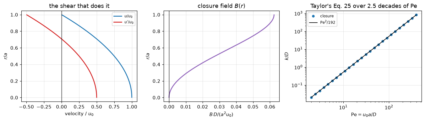
relative deviation from Eq. 25 over Pe = 2 to 398 (n_r = 160): -4.5775e-09 at every Pe, n_r^4 times it -3.000; spread across Pe (here 6e-13)The sweep over \(\mathrm{Pe}\) is an identity, not a test: the closure is linear in \(u'\), so \(B \propto \mathrm{Pe}\) and \(k \propto \mathrm{Pe}^2\) exactly, and its relative error is the same at every Peclet number, the grid error printed above, to round-off. The plot shows the scaling; the grid refinement in check 1 is what tests the closure.
And the direct simulation: a slug released across the section, seen in the frame moving at \(u_0/2\). It stays symmetric: that is Taylor’s observation, and it is not obvious from the parabolic velocity profile that produced it.
fig, axes = plt.subplots(1, 2, figsize=(11.4, 4.0))
_h = RUNS[1600]
for (tau, cm), col in zip(_h.profiles.items(), plt.cm.viridis(np.linspace(.15, .85, 4))):
    axes[0].plot(_h.slug.z_c, cm / cm.max(), color=col, lw=1.6, label=fr"$\tau$ = {tau}")
axes[0].set(xlabel=r"$(x - u_0 t/2)/a$", ylabel=r"section-mean $C_m/C_{m,\max}$",
            xlim=(-25, 25), title=r"the slug stays symmetric ($n_z$ = 1600)")
axes[0].legend(fontsize=8)
_s = RUNS[3200].slug
im = axes[1].pcolormesh(_s.z_c, _s.r_c, _s.c.reshape(_s.shape)[..., 0].T, cmap="magma",
                        shading="auto")
axes[1].set(xlabel=r"$(x - u_0 t/2)/a$", ylabel=r"$r/a$", xlim=(-25, 25),
            title=fr"the 2-D field at $\tau$ = {TAU_END}: radial gradients are small")
fig.colorbar(im, ax=axes[1], label=r"$C$ (unit total mass)")
fig.tight_layout()
plt.show()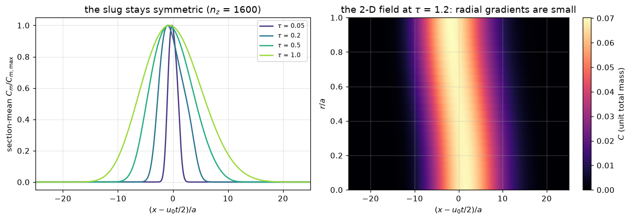
When Taylor’s result starts to hold
Taylor could only bound when Eq. 25 applies: wait “much longer than” the equilibration time \(a^2/(3.83^2 D)\). The modal series of the closure turns that inequality into a number. The first mode carries most of the deficit, so after a short start-up the deficit is one exponential, \(A\,\mathrm{e}^{-j_1^2\tau}\) with \(A = \alpha_1 k/(D+k)\), and the time after which the rate stays within a band \(b\) of Taylor’s value is close to \(\ln(A/b)/j_1^2\): every factor \(\mathrm{e}\) of accuracy costs one more equilibration time. The cell below computes the series (the closed forms stay in the notebook, apart from model.py) and the 2-D simulation checks it.
def modal_coefficients(n_modes=40, zeros_of=1):
    """Eigenvalues j_n^2 and weights alpha_n of the closure's modal series.

    ``zeros_of=1`` takes the zeros of J1, the no-flux tube. ``zeros_of=0`` takes
    the zeros of J0, the modes of an absorbing wall, which exists for the break
    table.
    """
    j = jn_zeros(zeros_of, n_modes)
    norm = np.array([np.sqrt(quad(lambda r: j0(z * r) ** 2 * 2 * r, 0, 1, limit=200)[0])
                     for z in j])
    beta = np.array([quad(lambda r: (0.5 - r * r) * j0(z * r) * 2 * r, 0, 1, limit=200)[0]
                     for z in j]) / norm
    return j ** 2, 192 * beta ** 2 / j ** 2


def modal_deviation(tau, Pe=PE_REF, coeffs=None):
    """Growth rate over Taylor's value, minus 1, from the modal series."""
    lam, alpha = modal_coefficients() if coeffs is None else coeffs
    k = Pe ** 2 / 192
    return -(k / (1 + k)) * np.sum(alpha * np.exp(-lam * np.atleast_1d(tau)[:, None]), axis=1)


def modal_settle(band, Pe=PE_REF, coeffs=None):
    """Settling time for a band: the root of |deviation| = band (it falls monotonically)."""
    coeffs = modal_coefficients() if coeffs is None else coeffs
    return brentq(lambda t: abs(modal_deviation(t, Pe, coeffs)[0]) - band, 1e-6, 10.0,
                  xtol=1e-14)


def modal_window_deficit(tau0, tau1, Pe=PE_REF, coeffs=None):
    """Mean of the deviation over a window, from the modal series."""
    lam, alpha = modal_coefficients() if coeffs is None else coeffs
    k = Pe ** 2 / 192
    return float(-(k / (1 + k)) * np.sum(alpha / lam * (np.exp(-lam * tau0)
                                                         - np.exp(-lam * tau1))) / (tau1 - tau0))


MODES = modal_coefficients()
J1SQ = float(MODES[0][0])
ALPHA1 = float(MODES[1][0])
A_MODAL = ALPHA1 * (TARGET - 1) / TARGET
TAU_MODAL = {b: modal_settle(b) for b in BANDS}
print(f"first mode: j_1^2 = {J1SQ:.4f}, alpha_1 = {ALPHA1:.5f} "
      f"(sum of 40 weights {np.sum(MODES[1]):.6f}), A = alpha_1 k/(D+k) = {A_MODAL:.5f}")
print(f"{'band':>8}{'tau (series)':>15}{'ln(A/b)/j_1^2':>16}{'equilibration times':>21}")
for b in BANDS:
    print(f"{100 * b:7.0f}%{TAU_MODAL[b]:15.5f}{np.log(A_MODAL / b) / J1SQ:16.5f}"
          f"{TAU_MODAL[b] / T_EQ:21.2f}")
first mode: j_1^2 = 14.6820, alpha_1 = 0.97066 (sum of 40 weights 1.000000), A = alpha_1 k/(D+k) = 0.90143
band tau (series) ln(A/b)/j_1^2 equilibration times
10% 0.14977 0.14976 2.20
5% 0.19698 0.19697 2.89
3% 0.23177 0.23177 3.40
2% 0.25938 0.25938 3.80
1% 0.30659 0.30659 4.50# The simulated growth rate on every rung against the series.
fig, axes = plt.subplots(1, 2, figsize=(11.6, 4.0))
_f = RUNS[3200]
axes[0].loglog(_f.t[1:], _f.variance[1:] - _f.variance[0], color="tab:blue", lw=1.9,
label="simulated, $n_z$ = 3200")
axes[0].loglog(_f.t[1:], 2 * TARGET * _f.t[1:], "k:", lw=1.4, label=r"Taylor $2(D+k)t$")
axes[0].axvline(T_EQ, color="tab:red", lw=1.2)
axes[0].text(T_EQ * 1.1, 1e-3, "Taylor's Eq. 16\nequilibration time", fontsize=8,
color="tab:red")
axes[0].set(xlabel=r"$\tau = tD/a^2$", ylabel=r"$(\sigma^2 - \sigma_0^2)/a^2$",
title="ballistic, then diffusive")
axes[0].legend(fontsize=8, loc="upper left")
for n_z, col in zip(N_Z_LADDER, ("0.85", "0.7", "0.5", "0.3", "tab:blue")):
h = RUNS[n_z]
axes[1].semilogx(h.t[1:], h.rate[1:] / TARGET, color=col, lw=1.0, label=f"$n_z$ = {n_z}")
_tt = np.logspace(-2.5, np.log10(TAU_END), 300)
axes[1].semilogx(_tt, 1 + modal_deviation(_tt), "k--", lw=1.3, label="modal series")
for band, st in ((0.05, ":"), (0.02, "--")):
axes[1].axhline(1 + band, color="tab:green", lw=0.9, ls=st)
axes[1].axhline(1 - band, color="tab:green", lw=0.9, ls=st)
axes[1].axvline(T_EQ, color="tab:red", lw=1.2)
axes[1].set(xlabel=r"$\tau = tD/a^2$", ylabel="growth rate / Taylor's value",
ylim=(0.8, 1.12), xlim=(0.05, TAU_END), title="when does Eq. 25 hold?")
axes[1].legend(fontsize=7, loc="lower right")
fig.tight_layout()
plt.show()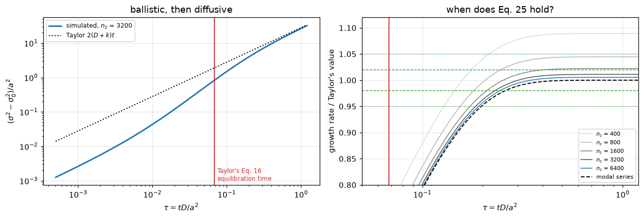
On every mesh the simulated rate settles above Taylor’s value, by a floor that halves with each doubling of \(n_z\): first-order upwind adds the numerical diffusivity \(\lvert u'\rvert\Delta z/2\) on every streamline, and its area mean, \(\langle\lvert u'\rvert\rangle = u_0/4\), enters the dispersion directly. A floor shifts every settling time: the rate enters a band from below, so it enters early by \(\ln(1 + \text{floor}/b)/\lambda\), and a band narrower than the floor is never entered at all. The settling check of the validation section measures both and removes the shift.
Validation
The checks are listed by the cell below. Then every number is registered as a claim, and a defect-injection table re-runs the computation behind each one with a defect in place.
CHECKS = ["the closure against Eq. 25, refined, with two choices of the mean",
          "the direct 2-D simulation against Eq. 25, refined, and its numerical-dispersion floor",
          "Taylor's worked capillary run",
          "the settling study, refined in dz, dt and n_r, against the modal series"]
print(f"{len(CHECKS)} checks:\n" + "\n".join(f"  {i + 1}. {c}" for i, c in enumerate(CHECKS)))
4 checks:
1. the closure against Eq. 25, refined, with two choices of the mean
2. the direct 2-D simulation against Eq. 25, refined, and its numerical-dispersion floor
3. Taylor's worked capillary run
4. the settling study, refined in dz, dt and n_r, against the modal series# 1. The closure against Taylor's closed form, refined, with the two choices of
# the mean, and the pinned cell moved from the axis to the wall.
EXACT = PE_REF ** 2 / 192
N_CL = (25, 50, 100, 200, 400, 800)
def closure_ladder(mean, **kw):
err = np.array([abs(closure(PE_REF, n_r=n, mean=mean, **kw).k_over_D / EXACT - 1)
for n in N_CL])
pin = np.array([abs(closure(PE_REF, n_r=n, mean=mean, pin=n - 1, **kw).k_over_D
- closure(PE_REF, n_r=n, mean=mean, **kw).k_over_D) / EXACT
for n in N_CL])
return err, pin
CL_DISC, PIN_DISC = closure_ladder("discrete")
CL_CONT, PIN_CONT = closure_ladder("continuous")
I200, I100 = N_CL.index(200), N_CL.index(100)
ORDER_DISC = float(np.log2(CL_DISC[I100] / CL_DISC[I200]))
ORDER_CONT = float(np.log2(CL_CONT[I100] / CL_CONT[I200]))
print("1. Closure against Eq. 25, Pe = 50, relative errors")
print(f" {'n_r':>5}{'grid mean':>13}{'pin moved':>12}{'u0/2 mean':>13}{'pin moved':>12}")
for i, n in enumerate(N_CL):
pin_disc = " < 1e-11" if PIN_DISC[i] < 1e-11 else f"{PIN_DISC[i]:12.1e}"
print(f" {n:5d}{CL_DISC[i]:13.2e}{pin_disc:>12}{CL_CONT[i]:13.2e}{PIN_CONT[i]:12.1e}")
print(f" observed order, n_r 100 to 200: {ORDER_DISC:.2f} with the grid's mean, "
f"{ORDER_CONT:.2f} with u0/2")
print(f" moving the pinned cell to the wall changes k by (here {PIN_DISC[I200]:.0e}) "
f"with the grid's mean, {PIN_CONT[I200]:.1e} with u0/2 (n_r = 200)")1. Closure against Eq. 25, Pe = 50, relative errors
n_r grid mean pin moved u0/2 mean pin moved
25 7.67e-06 < 1e-11 6.36e-03 9.5e-03
50 4.80e-07 < 1e-11 1.60e-03 2.4e-03
100 3.00e-08 < 1e-11 4.00e-04 6.0e-04
200 1.87e-09 < 1e-11 1.00e-04 1.5e-04
400 1.19e-10 < 1e-11 2.50e-05 3.7e-05
800 8.35e-12 < 1e-11 6.25e-06 9.4e-06
observed order, n_r 100 to 200: 4.00 with the grid's mean, 2.00 with u0/2
moving the pinned cell to the wall changes k by (here 1e-13) with the grid's mean, 1.5e-04 with u0/2 (n_r = 200)What check 1 shows. With the grid’s own mean subtracted, the closure reproduces Eq. 25 at fourth order, and the pinned cell changes \(k\) by round-off only; at \(n_r = 800\) the error has reached that round-off. With the exact mean \(u_0/2\), whose grid average is not zero, the singular system is inconsistent: the dropped equation is where the inconsistency goes, so moving the pin from the axis to the wall changes \(k\) by more than the whole error, and the error falls only at second order. The order is measured, not derived: the finite-volume scheme is formally second order, and the quadratic velocity profile cancels its leading error once the mean is consistent.
# 2. The direct 2-D simulation against Eq. 25, axial refinement at dt = 5e-4,
#    n_r = 24. The rate over a window [tau0, tau1] is the variance growth between
#    them. A window opened at tau = 0.2 still contains the start-up deficit; one
#    opened at 0.6 does not.
EARLY, LATE = (0.2, 1.0), (0.6, 1.2)
DIRECT = {n_z: {w: h.window_dispersion(*w) / TARGET - 1 for w in (EARLY, LATE)}
          for n_z, h in RUNS.items()}
FLOOR = {n_z: float(h.rate[-1] / TARGET - 1) for n_z, h in RUNS.items()}
MASS = {n_z: abs(h.mass[-1] / h.mass[0] - 1) for n_z, h in RUNS.items()}
COLSUM = float(np.max(np.abs(RUNS[3200].slug.column_sums())))
K24 = closure(PE_REF, n_r=N_R).k_over_D


def floor_closed_form(n_z):
    """Upwind's <|u'|> dz/2 = Pe dz/8, plus the 24-cell radial error of k, over D + k."""
    return (PE_REF * (80.0 / n_z) / 8 + K24 - EXACT) / TARGET


def richardson(x_coarse, x_fine):
    return 2 * x_fine - x_coarse                      # first order in dz


RICH_EARLY = richardson(DIRECT[3200][EARLY], DIRECT[6400][EARLY])
RICH_LATE = richardson(DIRECT[3200][LATE], DIRECT[6400][LATE])
MODAL_EARLY = modal_window_deficit(*EARLY)
MODAL_LATE = modal_window_deficit(*LATE)
print("2. Direct simulation against Eq. 25 (Pe = 50); D_eff/(D + k) - 1")
print(f"   {'n_z':>5}{'dz':>8}{'window 0.2-1.0':>16}{'window 0.6-1.2':>16}"
      f"{'floor at 1.2':>14}{'floor, closed form':>20}{'mass':>9}")
for n_z in N_Z_LADDER:
    print(f"   {n_z:5d}{80 / n_z:8.4f}{100 * DIRECT[n_z][EARLY]:15.3f}%"
          f"{100 * DIRECT[n_z][LATE]:15.3f}%{100 * FLOOR[n_z]:13.4f}%"
          f"{100 * floor_closed_form(n_z):19.4f}%   (here {MASS[n_z]:.0e})")
print(f"   Richardson limit (3200, 6400): window 0.2-1.0 {100 * RICH_EARLY:+.3f} % "
      f"(modal series {100 * MODAL_EARLY:+.3f} %), window 0.6-1.2 {100 * RICH_LATE:+.4f} % "
      f"(modal series {100 * MODAL_LATE:+.4f} %)")
FLOOR_ORDER = float(np.log2(FLOOR[3200] / FLOOR[6400]))
FLOOR_RATIO = FLOOR[3200] / floor_closed_form(3200)
print(f"   column sums of V^T J on n_z = 3200: max (here {COLSUM:.0e})")
print(f"   floor: observed order {FLOOR_ORDER:.3f} (3200 to 6400), "
      f"over its closed form at 3200 {FLOOR_RATIO:.5f}; radial part (k_24 - k)/(D + k) "
      f"{(K24 - EXACT) / TARGET:.1e}")
2. Direct simulation against Eq. 25 (Pe = 50); D_eff/(D + k) - 1
n_z dz window 0.2-1.0 window 0.6-1.2 floor at 1.2 floor, closed form mass
400 0.2000 8.499% 8.913% 8.9144% 8.9145% (here 6e-14)
800 0.1000 4.042% 4.455% 4.4568% 4.4568% (here 9e-14)
1600 0.0500 1.813% 2.226% 2.2280% 2.2280% (here 2e-14)
3200 0.0250 0.699% 1.112% 1.1136% 1.1136% (here 1e-13)
6400 0.0125 0.141% 0.555% 0.5564% 0.5564% (here 3e-13)
Richardson limit (3200, 6400): window 0.2-1.0 -0.416 % (modal series -0.407 %), window 0.6-1.2 -0.0024 % (modal series -0.0015 %)
column sums of V^T J on n_z = 3200: max (here 4e-15)
floor: observed order 1.001 (3200 to 6400), over its closed form at 3200 0.99999; radial part (k_24 - k)/(D + k) -8.4e-06What check 2 shows. Over the late window the simulation converges onto Eq. 25 at first order in \(\Delta z\): the extrapolated limit is zero to the accuracy of the modal start-up term. Over the window opened at \(\tau = 0.2\) it converges to a value below Eq. 25, and the modal series predicts that offset: it is the start-up deficit inside the window, not a failure of Eq. 25 and not numerical dispersion. The floor is upwind’s numerical dispersion in closed form, \(\mathrm{Pe}\,\Delta z/8\) over \(1 + \mathrm{Pe}^2/192\), plus the small radial error of the 24-cell grid. Mass is conserved to round-off because no boundary passes any flux: the column sums of the volume-weighted operator, \(V^{\mathsf T}J\), are zero to round-off, so \(\mathrm{d}M_0/\mathrm{d}t = 0\) for every state, not only for one that stays away from the ends.
# 3. Against Taylor's own measurement. His claim is that dispersion can be
#    inverted into a molecular diffusivity, so the test is whether the D implied
#    by his capillary run falls inside the independently measured range.
def taylor_inversion(a=TAY["tube_radius"], t=TAY["elapsed_time"], divisor=192.0):
    """k from his erf fit (4 k t = beta^-2), then D from Eq. 25."""
    k = 1.0 / (4.0 * t * TAY["erf_fit_parameter"] ** 2)
    return k, a ** 2 * TAY["centreline_velocity"] ** 2 / (divisor * k)


LO, HI = TAY["literature_diffusivity_min"], TAY["literature_diffusivity_max"]


def inside_margin(D):
    """Smallest relative distance of D to the ends of the measured range (negative outside)."""
    return min((D - LO) / LO, (HI - D) / HI)


K_FIT, D_INF = taylor_inversion()
PE_EXP = TAY["centreline_velocity"] * TAY["tube_radius"] / D_INF
print("3. Taylor's worked capillary run, recomputed")
print(f"   k from his erf fit   {K_FIT:8.4f} cm2/s   he prints {TAY['dispersion_coefficient']}")
print(f"   D from his Eq. 25    {D_INF:8.3e} cm2/s   he prints {TAY['inferred_diffusivity']:.2e}")
print(f"   relative agreement   k {100 * abs(K_FIT / TAY['dispersion_coefficient'] - 1):.2f} %, "
      f"D {100 * abs(D_INF / TAY['inferred_diffusivity'] - 1):.2f} %")
print(f"   independently measured range (Furth & Ullmann 1927, KMnO4, 18 C): "
      f"{LO:.3e} to {HI:.3e} cm2/s")
print(f"   inferred value lies inside it: {LO <= D_INF <= HI} "
      f"(margin {inside_margin(D_INF):.3f} relative to the nearer end)")
print(f"   Pe of that experiment = {PE_EXP:.0f}, so k/D = {PE_EXP ** 2 / 192:.0f}")
3. Taylor's worked capillary run, recomputed
k from his erf fit 0.1519 cm2/s he prints 0.152
D from his Eq. 25 5.977e-06 cm2/s he prints 6.00e-06
relative agreement k 0.04 %, D 0.38 %
independently measured range (Furth & Ullmann 1927, KMnO4, 18 C): 4.350e-06 to 1.500e-05 cm2/s
inferred value lies inside it: True (margin 0.374 relative to the nearer end)
Pe of that experiment = 2209, so k/D = 25420# 4. The settling study, refined in all three knobs.
# Raw: the root of the rate where it last leaves each band, per mesh.
# Corrected: raw + ln(1 + floor/b)/lam, the shift a constant floor causes when
# the rate enters the band from below; lam and A fitted on the run itself.
def settling(h):
floor = float(h.rate[-1] / TARGET - 1)
lam, A = h.fit_relaxation(TARGET, floor, *FIT_WINDOW)
raw, corr = {}, {}
for b in BANDS:
t = h.settle(TARGET, b)
raw[b] = t
if np.isfinite(t):
if not h.rate[int(t / (h.t[1] - h.t[0]))] < TARGET:
raise RuntimeError("the band is entered from above; the shift does not apply")
corr[b] = t + np.log(1 + floor / b) / lam
else:
corr[b] = np.nan
return {"floor": floor, "lam": lam, "A": A, "raw": raw, "corr": corr}
SET = {n_z: settling(h) for n_z, h in RUNS.items()}
SET_NR48, SET_DT2 = settling(RUN_NR48), settling(RUN_DT2)
def row(vals):
return "".join(" never" if not np.isfinite(vals[b]) else f"{vals[b]:11.5f}" for b in BANDS)
hdr = "".join(f"{f'+/-{100 * b:.0f}%':>11}" for b in BANDS)
print("4. Settling times; dz = 80/n_z")
print(f" {'':24}{hdr}{'lam':>10}{'A':>9}")
for n_z, s in SET.items():
print(f" raw n_z = {n_z:5d} {row(s['raw'])}{s['lam']:10.4f}{s['A']:9.5f}")
for n_z, s in SET.items():
print(f" corrected n_z = {n_z:5d} {row(s['corr'])}")
print(f" corrected, n_z = 800 at n_r = 48 {row(SET_NR48['corr'])}{SET_NR48['lam']:10.4f}")
print(f" corrected, n_z = 3200 at dt = 1e-3 {row(SET_DT2['corr'])}{SET_DT2['lam']:10.4f}")
print(f" modal series {row(TAU_MODAL)}{J1SQ:10.4f}{A_MODAL:9.5f}")
# corrected times from n_z = 3200, or from 6400 for a band the 3200 floor shuts out
FINEST = {b: 3200 if np.isfinite(SET[3200]["raw"][b]) else 6400 for b in BANDS}
CORR_BEST = {b: SET[FINEST[b]]["corr"][b] for b in BANDS}
CORR_VS_MODAL = {b: CORR_BEST[b] / TAU_MODAL[b] - 1 for b in BANDS}
SPREAD_3 = abs(SET[1600]["corr"][0.03] / SET[6400]["corr"][0.03] - 1)
SPREAD_10 = abs(SET[400]["corr"][0.10] / SET[6400]["corr"][0.10] - 1)
def raw_moves(sets):
"""Rise of every raw settling time per doubling of n_z, where both rungs enter the band."""
return [sets[N_Z_LADDER[i + 1]]["raw"][b] - sets[N_Z_LADDER[i]]["raw"][b]
for b in BANDS for i in range(len(N_Z_LADDER) - 1)
if np.isfinite(sets[N_Z_LADDER[i]]["raw"][b])]
RAW_MOVES = raw_moves(SET)
print(" corrected times taken from: " + ", ".join(f"{100 * b:.0f}% n_z = {FINEST[b]}" for b in BANDS))
print(f" corrected over the series - 1: "
+ ", ".join(f"{100 * b:.0f}% {100 * CORR_VS_MODAL[b]:+.2f} %" for b in BANDS))
print(f" the corrected +/-3 % time from n_z = 1600 and 6400 differs by {SPREAD_3:.1e} relative, "
f"the +/-10 % time from n_z = 400 and 6400 by {SPREAD_10:.1e}")
print(f" every raw time rises under refinement: smallest rise {min(RAW_MOVES):.5f} over "
f"{len(RAW_MOVES)} doublings")
def lam_be(n_r, dt):
"""Decay rate backward Euler gives the discrete slowest radial mode: ln(1 + lam_h dt)/dt."""
return float(np.log(1 + radial_eigenvalue(n_r) * dt) / dt)
LAM_H = radial_eigenvalue(N_R)
LAM_CASES = (("n_z = 3200", SET[3200]["lam"], N_R, DT),
("n_z = 3200, dt = 1e-3", SET_DT2["lam"], N_R, 2 * DT),
("n_z = 800, n_r = 48", SET_NR48["lam"], 2 * N_R, DT))
LAM_GAP = {lab: lam / lam_be(n, dt) - 1 for lab, lam, n, dt in LAM_CASES}
print(f" decay rate: j_1^2 = {J1SQ:.4f}; discrete radial eigenvalue on {N_R} cells "
f"{LAM_H:.4f}; backward Euler on it, ln(1 + lam_h dt)/dt:")
for lab, lam, n, dt in LAM_CASES:
print(f" {lab:24s} fitted {lam:.4f}, predicted {lam_be(n, dt):.4f}, "
f"fitted/predicted - 1 = {LAM_GAP[lab]:+.1e}")
LAM_SHARE = 1 - lam_be(N_R, DT) / J1SQ
print(f" predicted rate over j_1^2 - 1 at dt = {DT}, n_r = {N_R}: {-LAM_SHARE:+.4%}; "
f"corrected +/-3 % time over the series - 1: {CORR_VS_MODAL[0.03]:+.4%}")4. Settling times; dz = 80/n_z
+/-10% +/-5% +/-3% +/-2% +/-1% lam A
raw n_z = 400 0.10702 never never never never 14.5975 0.90146
raw n_z = 800 0.12541 0.15447 never never never 14.5975 0.90146
raw n_z = 1600 0.13687 0.17287 0.19506 never never 14.5975 0.90146
raw n_z = 3200 0.14341 0.18434 0.21148 0.23056 never 14.5975 0.90146
raw n_z = 6400 0.14693 0.19089 0.22146 0.24407 0.27807 14.5975 0.90146
corrected n_z = 400 0.15068 never never never never
corrected n_z = 800 0.15066 0.19812 never never never
corrected n_z = 1600 0.15065 0.19812 0.23311 never never
corrected n_z = 3200 0.15064 0.19812 0.23311 0.26089 never
corrected n_z = 6400 0.15064 0.19812 0.23311 0.26089 0.30837
corrected, n_z = 800 at n_r = 48 0.15042 0.19781 never never never 14.6207
corrected, n_z = 3200 at dt = 1e-3 0.15119 0.19884 0.23396 0.26184 never 14.5447
modal series 0.14977 0.19698 0.23177 0.25938 0.30659 14.6820 0.90143
corrected times taken from: 10% n_z = 3200, 5% n_z = 3200, 3% n_z = 3200, 2% n_z = 3200, 1% n_z = 6400
corrected over the series - 1: 10% +0.58 %, 5% +0.58 %, 3% +0.58 %, 2% +0.58 %, 1% +0.58 %
the corrected +/-3 % time from n_z = 1600 and 6400 differs by 5.7e-06 relative, the +/-10 % time from n_z = 400 and 6400 by 2.4e-04
every raw time rises under refinement: smallest rise 0.00352 over 10 doublings
decay rate: j_1^2 = 14.6820; discrete radial eigenvalue on 24 cells 14.6508; backward Euler on it, ln(1 + lam_h dt)/dt:
n_z = 3200 fitted 14.5975, predicted 14.5974, fitted/predicted - 1 = +8.6e-06
n_z = 3200, dt = 1e-3 fitted 14.5447, predicted 14.5445, fitted/predicted - 1 = +9.4e-06
n_z = 800, n_r = 48 fitted 14.6207, predicted 14.6206, fitted/predicted - 1 = +8.3e-06
predicted rate over j_1^2 - 1 at dt = 0.0005, n_r = 24: -0.5760%; corrected +/-3 % time over the series - 1: +0.5795%What check 4 shows. The raw settling times rise under every axial refinement, as a floor that shrinks with \(\Delta z\) requires. Corrected for the floor, the meshes agree with each other: the ±3 % time from 1600 and 6400 cells to 5.7e-6, the ±10 % time from 400 and 6400 cells to 2.4e-4, so the correction removes the axial error. What is left against the modal series is a bias of about half a per cent, the same in every band, and it is the decay rate: the 24-cell radial operator’s slowest eigenvalue \(\lambda_h\) lies below \(j_1^2\), and backward Euler damps that mode at \(\ln(1 + \lambda_h\Delta t)/\Delta t\) instead of \(\lambda_h\). That prediction matches the fitted rate to about \(10^{-5}\) at the reference step, at the doubled step and on 48 radial cells, and its shortfall against \(j_1^2\) equals the bias of the corrected times. The ±1 % band, which only the 6400-cell mesh can enter, carries the same bias.
Claims: what each number is, and how it is checked
Every number the page stands behind is registered once, in the cell below, with how it is checked (docs/claims-design.md in the gallery repository):
- a value is a result whose size is set by physics, by the data, by a closed form or by a discretisation. CI holds it to a relative tolerance of the committed baseline, 5 % unless the cell says otherwise;
- a bound is a quantity whose size is not physics: a round-off gap between two readings of one equation, a convergence order. It is checked against its stated limits on every run, on every machine, and states its basis;
- an exact result is a label, checked for equality, with its distance to the threshold that decided it.
Every claim has a row in the defect table below that fails its own check, so none is labelled structural.
def value(name, x, rtol=0.05, **kw):
    claims.value(name, x, rtol=rtol, **kw)


def bound(name, x, *, max=None, min=None, basis, note=None, structural=False):
    claims.bound(name, x, max=max, min=min, basis=basis, note=note, structural=structural)


# --- check 1: the closure ---------------------------------------------------------
value("closure_rel_err_n200", CL_DISC[I200], note="grid mean subtracted, n_r = 200")
bound("closure_order_grid_mean", ORDER_DISC, min=3.8, max=4.2, basis="chosen",
      note="measured fourth order, n_r 100 to 200; the scheme is formally second order")
bound("closure_pin_gap_grid_mean_n200", PIN_DISC[I200], max=1e-11, basis="identity",
      note="a consistent pure-Neumann system: the pinned cell cannot change k")
value("closure_u0half_rel_err_n200", CL_CONT[I200], note="exact mean u0/2 subtracted")
value("closure_u0half_pin_gap_n200", PIN_CONT[I200], note="pin at the wall instead of the axis")
bound("closure_order_u0half", ORDER_CONT, min=1.9, max=2.1, basis="theory",
      note="the grid mean of u - u0/2 is a second-order quadrature error")
value("closure_u0half_grid_mean_n200", float(np.sum(CL.w * u_dev_c) / PE_REF),
      note="grid area average of u - u0/2, over u0")
bound("closure_pe_sweep_spread", SWEEP_SPREAD, max=1e-11, basis="identity", structural=True,
      note="k is proportional to Pe^2 exactly (the closure is linear in u'), so the relative "
           "error is one number at every Pe; no defect of the closure changes that")
# --- check 2: the direct simulation ---------------------------------------------
value("direct_rel_err_n3200", DIRECT[3200][EARLY], note="window tau 0.2 to 1.0")
value("direct_richardson_rel_err", abs(RICH_EARLY), note="window 0.2 to 1.0, n_z 3200 and 6400")
value("modal_window_deficit_early", abs(MODAL_EARLY), rtol=1e-6, note="window 0.2 to 1.0")
value("direct_late_rel_err_n3200", DIRECT[3200][LATE], note="window tau 0.6 to 1.2")
value("direct_late_richardson_rel_err", RICH_LATE, rtol=0.2,
      note="window 0.6 to 1.2, n_z 3200 and 6400; the modal start-up term is -1.5e-5")
value("numerical_dispersion_floor_n3200", FLOOR[3200], rtol=1e-3)
value("floor_over_closed_form_n3200", FLOOR_RATIO, rtol=1e-4,
      note="floor over (Pe dz/8 + k_24 - k)/(D + k)")
bound("numerical_dispersion_order", FLOOR_ORDER, min=0.95, max=1.05, basis="theory",
      note="first-order upwind; n_z 3200 to 6400")
bound("mass_conservation_err", max(MASS.values()), max=1e-11, basis="identity",
      note="closed boundaries and a conservative scheme; worst over the five meshes")
bound("operator_column_sum_n3200", COLSUM, max=1e-11, basis="identity",
      note="V^T J = 0: no boundary passes flux, so dM0/dt = 0 for every state")
# --- check 3: Taylor's capillary run ---------------------------------------------
value("taylor_k_rel_err", abs(K_FIT / TAY["dispersion_coefficient"] - 1),
      note="k from his erf fit against the k he prints")
value("taylor_D_rel_err", abs(D_INF / TAY["inferred_diffusivity"] - 1))
claims.exact("taylor_D_inside_range", bool(LO <= D_INF <= HI), margin=inside_margin(D_INF),
             min_margin=0.05, note="relative distance to the nearer end of Furth & Ullmann's range")
value("taylor_pe_experiment", PE_EXP)
value("taylor_k_over_D_experiment", PE_EXP ** 2 / 192)
# --- the settling study ------------------------------------------------------------
for b in BANDS:
    p = f"{100 * b:.0f}pct"
    value(f"tau_settle_{p}_modal", TAU_MODAL[b], rtol=1e-6, note="modal series, 40 modes")
    value(f"tau_settle_{p}_corrected", CORR_BEST[b], rtol=1e-3,
          note=f"floor-corrected, n_z = {FINEST[b]}")
    value(f"tau_settle_{p}_corrected_vs_modal", CORR_VS_MODAL[b], rtol=0.05)
    if b >= 0.02:
        value(f"tau_settle_{p}_n3200", SET[3200]["raw"][b], rtol=1e-3, note="raw root, n_z = 3200")
value("tau_settle_3pct_mesh_spread", SPREAD_3, rtol=0.5,
      note="corrected time, n_z 1600 against 6400; a discretisation residual")
value("tau_settle_10pct_mesh_spread", SPREAD_10, rtol=0.5,
      note="corrected time, n_z 400 against 6400; a discretisation residual")
for lab, key in (("n_z = 3200", "relaxation_rate_vs_be_prediction"),
                 ("n_z = 3200, dt = 1e-3", "relaxation_rate_vs_be_prediction_dt1e-3"),
                 ("n_z = 800, n_r = 48", "relaxation_rate_vs_be_prediction_nr48")):
    value(key, LAM_GAP[lab], rtol=0.5,
          note=f"fitted decay rate over ln(1 + lam_h dt)/dt, minus 1, {lab}")
value("relaxation_rate_shortfall_n24", LAM_SHARE, rtol=1e-6,
      note="1 - ln(1 + lam_h dt)/(dt j_1^2) at dt = 5e-4, n_r = 24")
value("modal_alpha1", ALPHA1, rtol=1e-6, note="weight of the first radial mode")
value("modal_amplitude", A_MODAL, rtol=1e-6, note="alpha_1 k/(D + k) at Pe = 50")
value("relaxation_rate_n3200", SET[3200]["lam"], rtol=1e-3, note=f"fit on tau {FIT_WINDOW}")
value("relaxation_amplitude_vs_modal", SET[3200]["A"] / A_MODAL - 1, rtol=0.5,
      note="fitted A over the series' alpha_1 k/(D + k), minus 1")
claims.count("bands_entered_n3200", [b - SET[3200]["floor"] for b in BANDS], 0.0,
             min_margin=5e-4, relative=False,
             note="bands wider than the n_z = 3200 floor; margin in absolute deviation")
value("raw_time_smallest_rise", min(RAW_MOVES),
      note="smallest rise of a raw settling time per doubling of n_z, in a^2/D")
print(f"{len(claims.metrics)} claims: "
      + ", ".join(f"{sum(c['kind'] == k for c in claims.metrics.values())} {k}"
                  for k in ("value", "bound", "exact")))
54 claims: 45 value, 7 bound, 2 exactThe defect-injection table
Each row breaks one thing on purpose, re-runs the computation behind one or more claims with the defect in place (a changed argument of the same function, or one of the defect runs made in the implementation cell, never a typed number), and hands the result to claims.breaks, which records whether the claim’s own check (its tolerance or its bound) catches it. Every claim that is not structural must be failed by at least one row, and the last cell of the page raises otherwise.
BREAK = []


def brk(name, metric, broken):
    """One injected defect: ``broken`` is what claim ``metric`` becomes with it."""
    caught = claims.breaks(name, metric, broken)
    BREAK.append((name, metric, claims[metric], float(broken), caught))


# the closure
_nu0 = abs(closure(PE_REF, nu=0).k_over_D / EXACT - 1)
_nomean = abs(closure(PE_REF, subtract_mean=False).k_over_D / EXACT - 1)
brk("closure: nu = 0, a plane channel", "closure_rel_err_n200", _nu0)
brk("closure: full u on the right, mean not subtracted", "closure_rel_err_n200", _nomean)
_cl_e, _cl_p = CL_CONT, PIN_CONT          # the u0/2 ladder, computed in check 1
brk("closure: exact mean u0/2, not the grid's", "closure_order_grid_mean", ORDER_CONT)
brk("closure: exact mean u0/2, not the grid's", "closure_pin_gap_grid_mean_n200", _cl_p[I200])
brk("closure: exact mean u0/2, on 100 cells", "closure_u0half_rel_err_n200", _cl_e[I100])
brk("closure: exact mean u0/2, on 100 cells", "closure_u0half_pin_gap_n200", _cl_p[I100])
_nm_e, _ = closure_ladder("continuous", subtract_mean=False)
brk("closure: full u on the right, mean not subtracted", "closure_order_u0half",
    np.log2(_nm_e[I100] / _nm_e[I200]))
_rf200 = radial_grid(200)[0]
brk("closure: Cartesian weights dr in the grid mean", "closure_u0half_grid_mean_n200",
    np.sum(np.diff(_rf200) * u_dev_c) / PE_REF)
# the direct simulation
brk("2-D: n_z = 1600 instead of 3200", "direct_rel_err_n3200", DIRECT[1600][EARLY])
_wall_w = {w: richardson(RUN_WALL.window_dispersion(*w) / TARGET - 1,
                         RUN_WALL_6400.window_dispersion(*w) / TARGET - 1) for w in (EARLY, LATE)}
brk(f"2-D: wall uptake b = {WALL_B} on both rungs", "direct_richardson_rel_err", abs(_wall_w[EARLY]))
_m0 = modal_coefficients(zeros_of=0)
brk("series: modes of an absorbing wall (J0 zeros)", "modal_window_deficit_early",
    abs(modal_window_deficit(*EARLY, coeffs=_m0)))
brk("2-D: n_z = 1600 instead of 3200", "direct_late_rel_err_n3200", DIRECT[1600][LATE])
brk(f"2-D: wall uptake b = {WALL_B}", "direct_late_rel_err_n3200",
    RUN_WALL.window_dispersion(*LATE) / TARGET - 1)
brk(f"2-D: wall uptake b = {WALL_B} on both rungs", "direct_late_richardson_rel_err", _wall_w[LATE])
brk("2-D: n_z = 1600 instead of 3200", "numerical_dispersion_floor_n3200", FLOOR[1600])
_floor_wall = float(RUN_WALL.rate[-1] / TARGET - 1)
brk(f"2-D: wall uptake b = {WALL_B}", "numerical_dispersion_floor_n3200", _floor_wall)
brk(f"2-D: wall uptake b = {WALL_B}", "floor_over_closed_form_n3200",
    _floor_wall / floor_closed_form(3200))
brk(f"2-D: wall uptake b = {WALL_B} on both rungs", "numerical_dispersion_order",
    np.log2(_floor_wall / float(RUN_WALL_6400.rate[-1] / TARGET - 1)))
brk("2-D: open ends, upwind carries u'C through the end faces", "operator_column_sum_n3200",
    np.max(np.abs(Slug(PE_REF, n_z=3200, n_r=N_R, closed_ends=False).column_sums())))
brk(f"2-D: wall uptake b = {WALL_B}", "mass_conservation_err", abs(RUN_WALL.mass[-1] / RUN_WALL.mass[0] - 1))
# Taylor's capillary run
_kt, _ = taylor_inversion(t=420.0)
brk("Taylor: elapsed time 240 s read as 420 s", "taylor_k_rel_err",
    abs(_kt / TAY["dispersion_coefficient"] - 1))
_, _Da = taylor_inversion(a=0.0522)
_, _D48 = taylor_inversion(divisor=48.0)
brk("Taylor: tube radius 0.0252 read as 0.0522 cm", "taylor_D_rel_err",
    abs(_Da / TAY["inferred_diffusivity"] - 1))
brk("Taylor: Eq. 25 with the mean velocity, 192 -> 48", "taylor_D_rel_err",
    abs(_D48 / TAY["inferred_diffusivity"] - 1))
brk("Taylor: tube radius 0.0252 read as 0.0522 cm", "taylor_D_inside_range", bool(LO <= _Da <= HI))
brk("Taylor: Eq. 25 with the mean velocity, 192 -> 48", "taylor_D_inside_range",
    bool(LO <= _D48 <= HI))
brk("Taylor: tube radius 0.0252 read as 0.0522 cm", "taylor_pe_experiment",
    TAY["centreline_velocity"] * 0.0522 / _Da)
brk("Taylor: tube radius 0.0252 read as 0.0522 cm", "taylor_k_over_D_experiment",
    (TAY["centreline_velocity"] * 0.0522 / _Da) ** 2 / 192)
# the settling study
_tau_m0 = {b: modal_settle(b, coeffs=_m0) for b in BANDS}
for b in BANDS:
    p = f"{100 * b:.0f}pct"
    brk("series: modes of an absorbing wall (J0 zeros)", f"tau_settle_{p}_modal", _tau_m0[b])
    _s = SET[FINEST[b]]
    _slab = _s["raw"][b] + np.log(1 + _s["floor"] / b) / np.pi ** 2
    brk("floor shift with the slab eigenvalue pi^2", f"tau_settle_{p}_corrected", _slab)
    brk("floor shift with the slab eigenvalue pi^2", f"tau_settle_{p}_corrected_vs_modal",
        _slab / TAU_MODAL[b] - 1)
    if b >= 0.02:
        brk("2-D: dt = 1e-3 instead of 5e-4", f"tau_settle_{p}_corrected_vs_modal",
            SET_DT2["corr"][b] / TAU_MODAL[b] - 1)
        brk("2-D: dt = 1e-3 instead of 5e-4", f"tau_settle_{p}_n3200", SET_DT2["raw"][b])
_slab_sp = abs((SET[1600]["raw"][0.03] + np.log(1 + SET[1600]["floor"] / 0.03) / np.pi ** 2)
               / (SET[6400]["raw"][0.03] + np.log(1 + SET[6400]["floor"] / 0.03) / np.pi ** 2) - 1)
brk("floor shift with the slab eigenvalue pi^2", "tau_settle_3pct_mesh_spread", _slab_sp)
brk("series: modes of an absorbing wall (J0 zeros)", "modal_alpha1", _m0[1][0])
brk("series: modes of an absorbing wall (J0 zeros)", "modal_amplitude",
    _m0[1][0] * (TARGET - 1) / TARGET)
brk("2-D: dt = 1e-3 instead of 5e-4", "relaxation_rate_n3200", SET_DT2["lam"])
_set_wall = settling(RUN_WALL)
brk(f"2-D: wall uptake b = {WALL_B}", "relaxation_amplitude_vs_modal", _set_wall["A"] / A_MODAL - 1)
brk(f"2-D: wall uptake b = {WALL_B}", "relaxation_rate_vs_be_prediction",
    _set_wall["lam"] / lam_be(N_R, DT) - 1)
for key, n_r, dt in (("relaxation_rate_vs_be_prediction_dt1e-3", N_R, 2 * DT),
                     ("relaxation_rate_vs_be_prediction_nr48", 2 * N_R, DT)):
    # the fitted rate does not depend on n_z (check 4), so the wall run is on 800 cells
    _h = run_history(PE_REF, 800, dt=dt, n_r=n_r, tau_end=TAU_END, wall_b=WALL_B)
    brk(f"2-D: wall uptake b = {WALL_B} (n_z = 800, n_r = {n_r}, dt = {dt:g})", key,
        settling(_h)["lam"] / lam_be(n_r, dt) - 1)
brk("radial eigenvalue of the slab (nu = 0)", "relaxation_rate_shortfall_n24",
    1 - np.log(1 + radial_eigenvalue(N_R, nu=0) * DT) / (DT * J1SQ))
_slab10 = abs((SET[400]["raw"][0.10] + np.log(1 + SET[400]["floor"] / 0.10) / np.pi ** 2)
              / (SET[6400]["raw"][0.10] + np.log(1 + SET[6400]["floor"] / 0.10) / np.pi ** 2) - 1)
brk("floor shift with the slab eigenvalue pi^2", "tau_settle_10pct_mesh_spread", _slab10)
brk("2-D: n_z = 1600 instead of 3200", "bands_entered_n3200",
    int(sum(b > SET[1600]["floor"] for b in BANDS)))
brk("2-D: dt = 1e-3 instead of 5e-4 on the n_z = 3200 rung", "raw_time_smallest_rise",
    min(raw_moves({**SET, 3200: SET_DT2})))

print(f"{'injected defect':<56} {'claim':<38} {'clean':>16} {'broken':>16}  caught")
for name, metric, clean, broken, caught in BREAK:
    is_bound = claims.metrics[metric]["kind"] == "bound"
    shown = f"(here {clean:.1e})" if is_bound else f"{clean:10.4g}"
    broke = f"(here {broken:.1e})" if is_bound else f"{broken:10.4g}"
    print(f"{name[:56]:<56} {metric[:38]:<38} {shown:>16} {broke:>16}  "
          f"{'yes' if caught else 'NO'}")
_caught = {m for _, m, _, _, c in BREAK if c}
_structural = sorted(k for k, c in claims.metrics.items() if c.get("structural"))
_open = sorted(k for k in claims.metrics if k not in _caught and k not in _structural)
print(f"\n{len(BREAK)} rows; {len(_caught)} of {len(claims.metrics)} claims are failed by at "
      f"least one row; structural: {', '.join(_structural) or 'none'}; "
      f"open: {', '.join(_open) or 'none'}")
_uncaught = [(n, m) for n, m, _, _, c in BREAK if not c]
print("rows that do not fail their claim: " + (", ".join(f"{n} -> {m}" for n, m in _uncaught)
                                               or "none"))
injected defect claim clean broken caught
closure: nu = 0, a plane channel closure_rel_err_n200 1.875e-09 0.4666 yes
closure: full u on the right, mean not subtracted closure_rel_err_n200 1.875e-09 4 yes
closure: exact mean u0/2, not the grid's closure_order_grid_mean (here 4.0e+00) (here 2.0e+00) yes
closure: exact mean u0/2, not the grid's closure_pin_gap_grid_mean_n200 (here 1.1e-13) (here 1.5e-04) yes
closure: exact mean u0/2, on 100 cells closure_u0half_rel_err_n200 9.998e-05 0.0003997 yes
closure: exact mean u0/2, on 100 cells closure_u0half_pin_gap_n200 0.00015 0.0005997 yes
closure: full u on the right, mean not subtracted closure_order_u0half (here 2.0e+00) (here -1.3e-03) yes
closure: Cartesian weights dr in the grid mean closure_u0half_grid_mean_n200 6.25e-06 0.1667 yes
2-D: n_z = 1600 instead of 3200 direct_rel_err_n3200 0.006985 0.01813 yes
2-D: wall uptake b = 0.03 on both rungs direct_richardson_rel_err 0.004159 0.003398 yes
series: modes of an absorbing wall (J0 zeros) modal_window_deficit_early 0.004072 0.05275 yes
2-D: n_z = 1600 instead of 3200 direct_late_rel_err_n3200 0.01112 0.02226 yes
2-D: wall uptake b = 0.03 direct_late_rel_err_n3200 0.01112 0.01196 yes
2-D: wall uptake b = 0.03 on both rungs direct_late_richardson_rel_err -2.45e-05 0.000812 yes
2-D: n_z = 1600 instead of 3200 numerical_dispersion_floor_n3200 0.01114 0.02228 yes
2-D: wall uptake b = 0.03 numerical_dispersion_floor_n3200 0.01114 0.012 yes
2-D: wall uptake b = 0.03 floor_over_closed_form_n3200 1 1.078 yes
2-D: wall uptake b = 0.03 on both rungs numerical_dispersion_order (here 1.0e+00) (here 9.0e-01) yes
2-D: open ends, upwind carries u'C through the end faces operator_column_sum_n3200 (here 4.0e-15) (here 2.1e+00) yes
2-D: wall uptake b = 0.03 mass_conservation_err (here 3.5e-13) (here 6.9e-02) yes
Taylor: elapsed time 240 s read as 420 s taylor_k_rel_err 0.000404 0.4288 yes
Taylor: tube radius 0.0252 read as 0.0522 cm taylor_D_rel_err 0.003808 3.274 yes
Taylor: Eq. 25 with the mean velocity, 192 -> 48 taylor_D_rel_err 0.003808 2.985 yes
Taylor: tube radius 0.0252 read as 0.0522 cm taylor_D_inside_range 1 0 yes
Taylor: Eq. 25 with the mean velocity, 192 -> 48 taylor_D_inside_range 1 0 yes
Taylor: tube radius 0.0252 read as 0.0522 cm taylor_pe_experiment 2209 1067 yes
Taylor: tube radius 0.0252 read as 0.0522 cm taylor_k_over_D_experiment 2.542e+04 5924 yes
series: modes of an absorbing wall (J0 zeros) tau_settle_10pct_modal 0.1498 0.3559 yes
floor shift with the slab eigenvalue pi^2 tau_settle_10pct_corrected 0.1506 0.1541 yes
floor shift with the slab eigenvalue pi^2 tau_settle_10pct_corrected_vs_modal 0.00582 0.02895 yes
2-D: dt = 1e-3 instead of 5e-4 tau_settle_10pct_corrected_vs_modal 0.00582 0.009484 yes
2-D: dt = 1e-3 instead of 5e-4 tau_settle_10pct_n3200 0.1434 0.1439 yes
series: modes of an absorbing wall (J0 zeros) tau_settle_5pct_modal 0.197 0.4758 yes
floor shift with the slab eigenvalue pi^2 tau_settle_5pct_corrected 0.1981 0.2047 yes
floor shift with the slab eigenvalue pi^2 tau_settle_5pct_corrected_vs_modal 0.005801 0.0393 yes
2-D: dt = 1e-3 instead of 5e-4 tau_settle_5pct_corrected_vs_modal 0.005801 0.009458 yes
2-D: dt = 1e-3 instead of 5e-4 tau_settle_5pct_n3200 0.1843 0.185 yes
series: modes of an absorbing wall (J0 zeros) tau_settle_3pct_modal 0.2318 0.5641 yes
floor shift with the slab eigenvalue pi^2 tau_settle_3pct_corrected 0.2331 0.2435 yes
floor shift with the slab eigenvalue pi^2 tau_settle_3pct_corrected_vs_modal 0.005795 0.05049 yes
2-D: dt = 1e-3 instead of 5e-4 tau_settle_3pct_corrected_vs_modal 0.005795 0.009458 yes
2-D: dt = 1e-3 instead of 5e-4 tau_settle_3pct_n3200 0.2115 0.2123 yes
series: modes of an absorbing wall (J0 zeros) tau_settle_2pct_modal 0.2594 0.6342 yes
floor shift with the slab eigenvalue pi^2 tau_settle_2pct_corrected 0.2609 0.2754 yes
floor shift with the slab eigenvalue pi^2 tau_settle_2pct_corrected_vs_modal 0.005793 0.06179 yes
2-D: dt = 1e-3 instead of 5e-4 tau_settle_2pct_corrected_vs_modal 0.005793 0.009457 yes
2-D: dt = 1e-3 instead of 5e-4 tau_settle_2pct_n3200 0.2306 0.2314 yes
series: modes of an absorbing wall (J0 zeros) tau_settle_1pct_modal 0.3066 0.7541 yes
floor shift with the slab eigenvalue pi^2 tau_settle_1pct_corrected 0.3084 0.3229 yes
floor shift with the slab eigenvalue pi^2 tau_settle_1pct_corrected_vs_modal 0.005792 0.05314 yes
floor shift with the slab eigenvalue pi^2 tau_settle_3pct_mesh_spread 5.742e-06 0.05298 yes
series: modes of an absorbing wall (J0 zeros) modal_alpha1 0.9707 0.8435 yes
series: modes of an absorbing wall (J0 zeros) modal_amplitude 0.9014 0.7834 yes
2-D: dt = 1e-3 instead of 5e-4 relaxation_rate_n3200 14.6 14.54 yes
2-D: wall uptake b = 0.03 relaxation_amplitude_vs_modal 3.508e-05 -0.0001368 yes
2-D: wall uptake b = 0.03 relaxation_rate_vs_be_prediction 8.619e-06 -0.004745 yes
2-D: wall uptake b = 0.03 (n_z = 800, n_r = 24, dt = 0.0 relaxation_rate_vs_be_prediction_dt1e- 9.413e-06 -0.004757 yes
2-D: wall uptake b = 0.03 (n_z = 800, n_r = 48, dt = 0.0 relaxation_rate_vs_be_prediction_nr48 8.302e-06 -0.00473 yes
radial eigenvalue of the slab (nu = 0) relaxation_rate_shortfall_n24 0.00576 0.3304 yes
floor shift with the slab eigenvalue pi^2 tau_settle_10pct_mesh_spread 0.0002395 0.1258 yes
2-D: n_z = 1600 instead of 3200 bands_entered_n3200 4 3 yes
2-D: dt = 1e-3 instead of 5e-4 on the n_z = 3200 rung raw_time_smallest_rise 0.003522 0.003 yes
62 rows; 53 of 54 claims are failed by at least one row; structural: closure_pe_sweep_spread; open: none
rows that do not fail their claim: noneWhat pymrm adds
To Taylor’s result: nothing. Eq. 25 is right, the closure reproduces it, and the 2-D simulation converges onto it. His capillary run recomputes, and the diffusivity it implies lies inside the independently measured range.
To the question he left open, a number with two independent routes to it. Taylor could only say that his result holds once the slug has travelled “much longer than” the radial equilibration time. The page answers it twice: from the modal series of the closure (a derivation in this notebook, using scipy, not a library feature) and from the 2-D transient, assembled from pymrm’s construct_convflux_upwind, construct_grad and construct_div and solved on one factorisation. The two agree once the simulation’s numerical-dispersion floor is removed, to the time-step and radial-grid residual that check 4 measures. The cell below prints the numbers.
The answer is less demanding than “much longer than” suggests, and it has a simple form: within a band \(b\) of Taylor’s rate from about \(\ln(A/b)\) equilibration times, \(A \approx 0.9\) at this Peclet number, so each factor \(\mathrm{e}\) of accuracy costs one more equilibration time. In a reactor context this says that a lumped axial dispersion coefficient becomes safe once the residence time is a few radial diffusion times \(a^2/(3.83^2 D)\): a real restriction for a wide tube or a poorly diffusing solute, but not an order-of-magnitude margin.
What the page measures about the numerics. First-order upwind adds a floor to the simulated rate, in closed form \(\mathrm{Pe}\,\Delta z/8\) over \(1 + \mathrm{Pe}^2/192\), and a floor biases every settling time low, because the rate enters a band from below. A band narrower than the floor is never entered at all, however long the run. Refinement removes the floor only in the limit, at first order; a scheme without numerical dispersion would remove it at the source. On this page the floor shift \(\ln(1 + \text{floor}/b)/\lambda\) removes it from each mesh’s settling times, and the corrected times agree across the five meshes.
print("The numbers behind the paragraphs above, from the cells that computed them:")
for b in BANDS:
    p = f"{100 * b:.0f}pct"
    print(f"  +/-{100 * b:2.0f} %: series tau = {claims[f'tau_settle_{p}_modal']:.4f} "
          f"({claims[f'tau_settle_{p}_modal'] / T_EQ:.2f} equilibration times), "
          f"simulation corrected {claims[f'tau_settle_{p}_corrected']:.4f} "
          f"({100 * claims[f'tau_settle_{p}_corrected_vs_modal']:+.2f} %)"
          + (f", raw on n_z = 3200 {claims[f'tau_settle_{p}_n3200']:.4f}" if b >= 0.02 else ""))
print(f"  A = alpha_1 k/(D + k) = {A_MODAL:.4f}; the floor on n_z = 3200 is "
      f"{100 * claims['numerical_dispersion_floor_n3200']:.3f} %, "
      f"{claims['floor_over_closed_form_n3200']:.5f} of its closed form")
The numbers behind the paragraphs above, from the cells that computed them:
+/-10 %: series tau = 0.1498 (2.20 equilibration times), simulation corrected 0.1506 (+0.58 %), raw on n_z = 3200 0.1434
+/- 5 %: series tau = 0.1970 (2.89 equilibration times), simulation corrected 0.1981 (+0.58 %), raw on n_z = 3200 0.1843
+/- 3 %: series tau = 0.2318 (3.40 equilibration times), simulation corrected 0.2331 (+0.58 %), raw on n_z = 3200 0.2115
+/- 2 %: series tau = 0.2594 (3.80 equilibration times), simulation corrected 0.2609 (+0.58 %), raw on n_z = 3200 0.2306
+/- 1 %: series tau = 0.3066 (4.50 equilibration times), simulation corrected 0.3084 (+0.58 %)
A = alpha_1 k/(D + k) = 0.9014; the floor on n_z = 3200 is 1.114 %, 0.99999 of its closed formReuse
The closure is the reusable part. closure in model.py needs only a velocity profile and a geometry; it is not specific to Poiseuille flow. Swap velocity_deviation for a turbulent profile, an annulus or a packed-bed velocity distribution and the same few lines give that geometry’s dispersion coefficient. Subtract the mean on the grid (sum(w * u)), so that the pinned singular system is consistent; check 1 shows what the exact mean costs. Changing nu=1 to nu=0 gives the plane channel, whose analytic answer is \(k = 2\bar u^2 h^2/105D\); the area weights w must then change with it, which radial_grid does not do.
Where this feeds the rest of the gallery. Every axial-dispersion coefficient in an S4 model (breakthrough curves, tracer RTDs, J1.5 adsorption) is a lumped stand-in for this calculation. This page is what justifies the lumping, and the modal series says when: within a band \(b\) after about \(\ln(0.9/b)/3.83^2\) radial diffusion times \(a^2/D\) for a slug released across the section. A release concentrated near the axis changes the amplitudes and needs its own series.
Do not read a settling time off one mesh. The criterion “the growth rate stays within a band” is met sooner on a coarse grid, because first-order upwind lifts the whole curve above the target by a floor proportional to \(\Delta z\), and a band narrower than that floor is never entered. Check the floor against its closed form, \(\langle\lvert u'\rvert\rangle\Delta z/2\) over the target, and correct for it, or use a scheme without numerical dispersion.
Careful with the velocity convention. \(u_0\) here is the centreline value, as in Taylor’s paper. Using the mean velocity in Eq. 25 without changing 192 to 48 gives an answer four times too small; the break table shows what that does to Taylor’s inferred diffusivity.
Related pages. A2.1 closes the dispersion model this page justifies; A4.9 (multicomponent diffusion); D2.2 (the plug-flow limit this relaxes); J1.5.
Cite the source, not this page: Taylor, G. I., Dispersion of soluble matter in solvent flowing slowly through a tube, Proc. R. Soc. Lond. A 219(1137) 186-203 (1953), doi:10.1098/rspa.1953.0139.
# Claims: every registered number printed, agreement.json written for CI, and an
# exception raised when a claim fails its own check or has no break row.
claims.says("2.2e3", "taylor_pe_experiment")            # Parameters and assumptions
claims.says("2.5e4", "taylor_k_over_D_experiment")      # Parameters and assumptions
claims.says("0.9", "modal_amplitude")                   # What pymrm adds, Reuse
claims.says("5.7e-6", "tau_settle_3pct_mesh_spread")    # check 4
claims.says("2.4e-4", "tau_settle_10pct_mesh_spread")   # check 4
claims.report();   # the semicolon keeps the notebook from echoing the payload
Claims for A2.3:
closure_rel_err_n200 = 1.875e-09 value rtol 0.05
closure_order_grid_mean = (here 4.0e+00) bound bound [3.8, 4.2] [chosen]
closure_pin_gap_grid_mean_n200 = (here 1.1e-13) bound bound <= 1e-11 [identity]
closure_u0half_rel_err_n200 = 9.9981e-05 value rtol 0.05
closure_u0half_pin_gap_n200 = 0.00014998 value rtol 0.05
closure_order_u0half = (here 2.0e+00) bound bound [1.9, 2.1] [theory]
closure_u0half_grid_mean_n200 = 6.25e-06 value rtol 0.05
closure_pe_sweep_spread = (here 6.3e-13) bound bound <= 1e-11 [identity]
direct_rel_err_n3200 = 0.0069854 value rtol 0.05
direct_richardson_rel_err = 0.0041586 value rtol 0.05
modal_window_deficit_early = 0.0040719 value rtol 1e-06
direct_late_rel_err_n3200 = 0.011119 value rtol 0.05
direct_late_richardson_rel_err = -2.4498e-05 value rtol 0.2
numerical_dispersion_floor_n3200 = 0.011136 value rtol 0.001
floor_over_closed_form_n3200 = 0.99999 value rtol 0.0001
numerical_dispersion_order = (here 1.0e+00) bound bound [0.95, 1.05] [theory]
mass_conservation_err = (here 3.5e-13) bound bound <= 1e-11 [identity]
operator_column_sum_n3200 = (here 4.0e-15) bound bound <= 1e-11 [identity]
taylor_k_rel_err = 0.00040401 value rtol 0.05
taylor_D_rel_err = 0.0038079 value rtol 0.05
taylor_D_inside_range = True exact exact, margin 0.374
taylor_pe_experiment = 2209.2 value rtol 0.05
taylor_k_over_D_experiment = 25420 value rtol 0.05
tau_settle_10pct_modal = 0.14977 value rtol 1e-06
tau_settle_10pct_corrected = 0.15064 value rtol 0.001
tau_settle_10pct_corrected_vs_modal = 0.0058201 value rtol 0.05
tau_settle_10pct_n3200 = 0.14341 value rtol 0.001
tau_settle_5pct_modal = 0.19698 value rtol 1e-06
tau_settle_5pct_corrected = 0.19812 value rtol 0.001
tau_settle_5pct_corrected_vs_modal = 0.0058009 value rtol 0.05
tau_settle_5pct_n3200 = 0.18434 value rtol 0.001
tau_settle_3pct_modal = 0.23177 value rtol 1e-06
tau_settle_3pct_corrected = 0.23311 value rtol 0.001
tau_settle_3pct_corrected_vs_modal = 0.0057946 value rtol 0.05
tau_settle_3pct_n3200 = 0.21148 value rtol 0.001
tau_settle_2pct_modal = 0.25938 value rtol 1e-06
tau_settle_2pct_corrected = 0.26089 value rtol 0.001
tau_settle_2pct_corrected_vs_modal = 0.0057934 value rtol 0.05
tau_settle_2pct_n3200 = 0.23056 value rtol 0.001
tau_settle_1pct_modal = 0.30659 value rtol 1e-06
tau_settle_1pct_corrected = 0.30837 value rtol 0.001
tau_settle_1pct_corrected_vs_modal = 0.0057918 value rtol 0.05
tau_settle_3pct_mesh_spread = 5.7423e-06 value rtol 0.5
tau_settle_10pct_mesh_spread = 0.0002395 value rtol 0.5
relaxation_rate_vs_be_prediction = 8.6193e-06 value rtol 0.5
relaxation_rate_vs_be_prediction_dt1e-3 = 9.4132e-06 value rtol 0.5
relaxation_rate_vs_be_prediction_nr48 = 8.3024e-06 value rtol 0.5
relaxation_rate_shortfall_n24 = 0.0057597 value rtol 1e-06
modal_alpha1 = 0.97066 value rtol 1e-06
modal_amplitude = 0.90143 value rtol 1e-06
relaxation_rate_n3200 = 14.598 value rtol 0.001
relaxation_amplitude_vs_modal = 3.508e-05 value rtol 0.5
bands_entered_n3200 = 4 exact exact, margin 0.00114
raw_time_smallest_rise = 0.0035221 value rtol 0.05