# Bootstrap: the pymrm this page was checked with, and the gallery files it was
# published with. Works in a checkout, in CI and on a fresh Colab VM.
GALLERY_REF = "gallery-2026.11.10.3"  # replaced by the release tag at publication
PYMRM = ">=3.4.0,<4"  # equals meta.yaml pymrm_min_version, up to the next major
PAGE = "D2.2-van-welsenaere-froment-runaway"  # equals the page directory

import os, sys, urllib.request
from pathlib import Path
_shared = next((p / "shared" for p in (Path.cwd(), *Path.cwd().parents)
                if (p / "shared" / "gallery_bootstrap.py").is_file()), None)
if _shared is None:
    _shared = (Path(os.environ.get("XDG_CACHE_HOME") or Path.home() / ".cache")
               / "pymrm-gallery" / GALLERY_REF)
    _shared.mkdir(parents=True, exist_ok=True)
    urllib.request.urlretrieve(
        "https://raw.githubusercontent.com/computational-chemical-engineering/"
        f"pymrm-gallery/{GALLERY_REF}/shared/gallery_bootstrap.py",
        _shared / "gallery_bootstrap.py")
sys.path.insert(0, str(_shared))
sys.modules.pop("gallery_bootstrap", None)
from gallery_bootstrap import setup
setup(PAGE, PYMRM, GALLERY_REF); # the semicolon stops the cell echoing the pathParametric sensitivity and runaway in a fixed bed
sec:D
struct:S2
tier:T0
data:tier6
phase:gas-solid
Two 1970 criteria for when a cooled tubular reactor stops being controllable, rebuilt, then swept over the whole operating plane the original could only sample.
Parametric sensitivity and runaway in a fixed bed
Catalog ID: D2.2 · Structures: S2 (plug flow with reaction) · Tier: T0
An exothermic reaction in a cooled tube always makes a hot spot. Raise the inlet concentration a few percent and the hot spot may rise a few degrees, or it may rise by hundreds. There is a boundary, and Van Welsenaere and Froment found two ways to locate it without integrating anything.
from dataclasses import replace

import numpy as np
import pandas as pd
import matplotlib.pyplot as plt
from scipy.optimize import brentq
from gallery_utils import load_data, load_meta, cite_data, Claims
from model import (VWFCase, kexp, maxima_curve, ps_curve, t_max_peak, t_tangency,
                   inlet_limits, back_integrate, critical_points, RunawayTube,
                   critical_p0, critical_p0_bisect)

plt.rcParams.update({"figure.dpi": 110, "axes.grid": True, "grid.alpha": 0.3})
claims = Claims(PAGE.split("-")[0])
Background
Put an exothermic reaction in a tube with a cooled wall and the temperature profile has a maximum. Where that maximum sits is a design question with consequences: too hot and the catalyst sinters, the selectivity collapses, or the tube itself creeps. What makes it hard is that the hot spot is not merely sensitive to the operating variables: over part of the range it is violently sensitive. In the base case of this paper at \(T_w\) = 625 K, 5 % more inlet pressure from 0.0164 atm raises the hot spot by 7.47 K, while 1 % more from 0.0182 atm raises it by 304 K (both computed below, converged in the grid; on the page’s default 1500 cells they are 7.4 K and 304 K).
Before 1970 there were two ways to deal with this. Bilous and Amundson (1956) perturbed a known steady state, which requires having integrated the reactor first. Barkelew (1959) integrated a very large number of cases and condensed the results into an empirical chart, which requires trial and error to use and is tied to his modified rate expression.
Van Welsenaere and Froment did something different: they looked for intrinsic features of the solution, characteristic points that exist in the temperature profile whether or not anyone has computed it, and translated them into the p–T phase plane, where they become geometry. The result is a set of closed-form inequalities on the inlet conditions. No computer, which in 1970 was the point.
Note the terminology, which they are careful about: with gas and solid at the same temperature, an ideal tubular reactor is always stable in the strict sense. There is no bifurcation here. “Runaway” is a statement about sensitivity, not about multiplicity, which is what distinguishes this page from B1.1, where the multiplicity is real.
The published model
Reactor (their Eqs. 3–4). One dimension, pseudo-homogeneous, constant wall temperature, single irreversible pseudo-first-order reaction:
\[ \frac{\mathrm{d}p}{\mathrm{d}z} = -A\,p\,\mathrm{e}^{-a/T+b}, \qquad \frac{\mathrm{d}T}{\mathrm{d}z} = B\,p\,\mathrm{e}^{-a/T+b} - C\,(T-T_w), \]
\[ A = \frac{M P \rho_b}{\rho_g} p_B^0, \qquad B = \frac{(-\Delta H)\rho_b}{c_p} p_B^0, \qquad C = \frac{2U}{c_p R}, \qquad z = \frac{z'}{u}, \]
with \(p = p^0\) and \(T = T_0 = T_w\) at \(z = 0\). The axial coordinate is a contact time, not a length.
The p–T plane. Dividing one equation by the other removes \(z\) altogether, so every reactor is a single trajectory in the \((T, p)\) plane. Two loci live in that plane and neither depends on the inlet conditions:
- the maxima curve (Eq. 7), where \(\mathrm{d}T/\mathrm{d}z = 0\): \(p_m = (T_m - T_w) \big/ \left[\tfrac{B}{C}\mathrm{e}^{-a/T_m+b}\right]\);
- the \(p_s\) curve (Eq. 18), the locus of the inflexion points that appear before the maximum: \(p_s = T_i^2 \big/ \left[a\tfrac{B}{C}\mathrm{e}^{-a/T_i+b}\right]\).
First criterion. The maxima curve has a maximum of its own, at
\[ T_M = \tfrac{1}{2}\left[a - \sqrt{a\,(a - 4T_w)}\right] \qquad (8) \]
A trajectory that crosses the maxima curve beyond its peak is one where a further small increase in \(p^0\) moves the hot spot sharply. So: the trajectory through the maximum of the maxima curve is critical.
Second criterion. An inflexion point before the maximum is what makes the hot spot grow. So: the critical trajectory is the one tangent to the \(p_s\) curve. The tangency condition reduces to one implicit equation in \(t = a/T_i\) (Eq. 20),
\[ K = \frac{t-2}{t\,\mathrm{e}^{-t+20}}\left[1 - t\left(1 - \frac{t}{t_w}\right)\right], \qquad K = \frac{A}{C}\mathrm{e}^{b-20}, \quad t_w = \frac{a}{T_w}, \]
which the paper solves graphically, through its Figs. 6 and 7, to avoid needing a computer.
From the critical point to the inlet. Both criteria give a critical \((T_{cr}, p_{cr})\) inside the reactor; getting back to the inlet needs an extrapolation, and the paper gives a lower and an upper limit rather than one value:
\[ (p^0)_l = \frac{T_{cr}^2}{a\frac{B}{C}\mathrm{e}^{-a/T_{cr}+b}} + \frac{A}{B}(T_{cr}-T_0) \quad (27), \qquad (p^0)_u = \frac{A}{B}(T_{cr}-T_w)\left[\frac{1}{\sqrt{X}} + 1\right]^2 \quad (28), \]
with \(X = \frac{A}{C}\mathrm{e}^{-a/T_{cr}+b}\). Their empirical observation, the one that makes the method usable, is that the mean of the two limits is an excellent estimate of the true critical inlet pressure, and for the first criterion that mean has the closed form (30)
\[ (p^0)_m = \frac{A}{B}(T_M-T_w)\left[1 + \frac{1}{\sqrt{X}} + \frac{1}{X}\right]. \]
Parameters and assumptions
Assumptions: one dimension, no axial dispersion; pseudo-homogeneous, so gas and solid share a temperature; constant wall temperature; constant fluid density and velocity; a single irreversible reaction, pseudo-first-order in the limiting reactant with the second reactant in excess at \(p_B^0\); ideal gas.
One trap in this paper, and it is a units trap. \(c_p\) is printed as kcal/m³·°C: it is already a volumetric heat capacity. Multiplying it by \(\rho_g\) “to fix the units” changes \(B\) and \(C\) by that factor and moves the runaway boundary with no other symptom; the break table below runs it. \(\rho_g\) appears only in \(A\).
One trap in getting the numbers out. This is a 1970 scan and the Elsevier full-text API returns the publisher’s OCR of it, which discards the mid-dot decimal separator: R = 00125 m for 0.0125 m, b = 19837 for 19.837, 001353 for 0.01353 atm. The API is excellent for prose and useless for numbers. Everything below was read from a 600 dpi render of the printed page, and the validation section shows the check that the reading is right.
par = load_data("van-welsenaere-froment-1970-parameters.csv", page=PAGE)
print(par.to_string(index=False))

CASE = VWFCase.from_table(zip(par.symbol, par.value))
TW = 625.0                     # K, the wall (and inlet) temperature of Examples 1 and 2
print(f"\nA = {CASE.A:.6g} 1/hr,  B = {CASE.B:.6g} K/(hr atm),  C = {CASE.C:.6g} 1/hr")
symbol value unit description
M 29.4800 kg/kmol mean molecular weight
P 1.0000 atm total pressure
rho_b 1300.0000 kg/m3 catalyst bulk density
rho_g 1.2930 kg/m3 gas density
minus_dH 307000.0000 kcal/kmol heat of reaction
c_p 0.3230 kcal/(m3 degC) volumetric heat capacity of the gas
u 3600.0000 m/hr superficial velocity
U 82.7000 kcal/(m2 hr degC) overall wall heat transfer coefficient
R 0.0125 m tube radius (base case; varied in Example 4)
p_B0 0.2080 atm partial pressure of the second reactant (in excess)
a 13636.0000 1/K activation energy over the gas constant, E/R
b 19.8370 - logarithm of the frequency factor
A = 6165.04 1/hr, B = 2.57006e+08 K/(hr atm), C = 40965.9 1/hrThe data
Two datasets. The parameters are the base case of their Section 1. The examples are every number printed in their Section 6: four worked problems, including the intermediate steps, so a reimplementation can be checked stage by stage rather than only at the answer.
These are not measurements. The paper contains no experimental data at all; its numbers are partly closed-form extrapolations and partly its own fourth-order Runge–Kutta integrations. This page is therefore provenance tier 6, validated against a published reference solution in the same sense as B1.1 and F3.1. The kind column separates the two, because a criterion value and an integration value test different things and should not be pooled.
ex = load_data("van-welsenaere-froment-1970-examples.csv", page=PAGE)
ex_meta = load_meta("van-welsenaere-froment-1970-examples.csv", page=PAGE)


def paper(example, quantity):
    """A value printed in Section 6, read from the examples CSV."""
    hit = ex[(ex.example == example) & (ex.quantity == quantity)]
    return float(hit.value.iloc[0])


print(ex.groupby(["example", "kind"]).size().unstack(fill_value=0).to_string())
print(f"\n{cite_data(ex_meta)}")
print(f"provenance tier {ex_meta['provenance_tier']['tier']}: "
      + " ".join(ex_meta["provenance_tier"]["note"].split())[:96] + " ...")
kind criterion integration
example
1a 4 1
1b 10 1
2 1 2
3 4 1
4 6 0
Van Welsenaere, R. J.; Froment, G. F. (1970) — Chemical Engineering Science 25(10) 1503-1516 — doi:10.1016/0009-2509(70)85073-4 — table
provenance tier 6: THESE ARE NOT MEASUREMENTS. They are the authors' own computed values - partly closed-form extra ...PyMRM implementation
Two pieces, both in model.py next to this notebook. The reactor, RunawayTube, is convection with a source in the contact time \(z\): construct_convflux_upwind then construct_div, the same two calls as C2.1, with the state \((p, T)\) on a (n_z, 2) grid and the source differentiated per cell by NumJac. The inlet values enter through shapes_d, so changing the inlet pressure changes one vector and no operator. The criteria (t_max_peak, t_tangency, inlet_limits) are algebra on the groups \(A\), \(B\), \(C\) and touch no operator at all; back_integrate is the paper’s own definition of the exact critical inlet pressure, a phase-plane quadrature with solve_ivp.
Three implementation choices are worth stating.
Newton is bounded, scaled and checked. RunawayTube.solve calls newton with bounds keeping \(T > 0\), where the Arrhenius factor is defined, with the step test scaled by the inlet values (scale), so \(p\) in atm and \(T\) in K are each judged against their own size, and it raises when Newton does not converge. Past the critical inlet pressure the solution is still bounded, and the differential equations, an initial-value problem in \(z\), have one solution per inlet pressure. The discrete system need not: on 1500 cells some backward-Euler cells near the inlet have further, ignited roots in the runaway region. Newton started from the solution at a neighbouring inlet pressure follows the low root, the one that converges to the differential solution under refinement, and the page checks every traced state against an independent solve (Validation).
The critical inlet pressure is a root. The reactor’s hot spot rises monotonically with \(p^0\), so the critical value is the root of \(T_{\max}(p^0) - T_M\), found by brentq on independent solves from the inlet state. The bracket starts from the paper’s own Eq. 27 and Eq. 30 values; Eq. 30 is an estimate, not a bound, so critical_p0 raises its upper end by 1 % at a time until the root is bracketed. pymrm.continuation does not fit this step: it follows a solution branch over parameter values given in advance and does not locate the value at which a functional of the solution reaches a target; and every solve in the bracket converges from the inlet state, so pseudo_transient has nothing to do. Bisection on the same bracket is kept as a second route (Validation).
The hot spot against \(p^0\) is a continuation. Sweeping the inlet pressure is what pymrm.continuation is for (RunawayTube.trace_inlet), with its branch-jump check at its default: a correction that moves the state by more than 20 % of its largest value away from the secant prediction is rejected and the sub-step is halved. Past the critical pressure the hot spot moves upstream, and the march reaches every requested value; every traced state is checked against an independent solve (Validation).
Results
The paper’s Figs. 1 and 2 are the sensitivity itself: a set of profiles at inlet pressures that differ by a few percent. Below, the same sweep, with the critical value marked.
TM_625 = t_max_peak(CASE, TW)
CP_625 = critical_points(CASE, TW)
LO_625, UP_625, MEAN_625 = inlet_limits(CASE, TM_625, TW)
P_CRIT = critical_p0(CASE, TW, LO_625, MEAN_625)       # pymrm reactor, criterion 1
levels = [0.008, 0.012, 0.0145, 0.0158, 0.0164, P_CRIT, 0.0168, 0.0172]

fig, axes = plt.subplots(1, 2, figsize=(11.5, 4.3))
cmap = plt.cm.viridis(np.linspace(0.05, 0.92, len(levels)))
tubes = {}
for p0, col in zip(levels, cmap):
    m = tubes[p0] = RunawayTube(CASE, p0, TW).solve()
    z_m = m.z_c * CASE.u                       # back to metres for the plot
    crit = p0 == P_CRIT
    kw = dict(color="tab:red" if crit else col, lw=2.2 if crit else 1.4,
              zorder=5 if crit else 2)
    axes[0].plot(z_m, m.p, **kw)
    axes[1].plot(z_m, m.T, label=f"{p0*1000:.2f}" + (" (critical)" if crit else ""),
                 **kw)
axes[0].set(xlabel="z' (m)", ylabel="p (atm)", xlim=(0, 1))
axes[1].set(xlabel="z' (m)", ylabel="T (K)", xlim=(0, 1))
axes[1].axhline(TM_625, color="k", ls="--", lw=0.9)
axes[1].text(0.985, TM_625 + 0.7, r"$T_M$ (Eq. 8)", fontsize=8, ha="right")
axes[1].legend(title=r"$p^0$ (10$^{-3}$ atm)", fontsize=8, loc="lower right",
               ncol=2)
fig.suptitle(f"Parametric sensitivity at $T_w$ = {TW:.0f} K "
             f"(their Figs. 1 and 2, rebuilt)", fontsize=11)
fig.tight_layout()
plt.show()

print(f"critical inlet partial pressure at Tw = {TW:.0f} K, pymrm reactor: {P_CRIT:.5f} atm")
print(f"paper, by back-integration from the critical point:      "
      f"{paper('1a', 'p0_critical'):.5f} atm")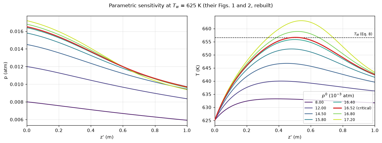
critical inlet partial pressure at Tw = 625 K, pymrm reactor: 0.01652 atm
paper, by back-integration from the critical point:      0.01651 atm
The whole argument is easier to see in the p–T plane, where the trajectories are inlet-independent geometry against two fixed curves.
fig, ax = plt.subplots(figsize=(6.6, 4.8))
Tgrid = np.linspace(TW + 0.4, 700.0, 400)
ax.plot(Tgrid, maxima_curve(CASE, Tgrid, TW), "k-", lw=1.6, label="maxima curve (Eq. 7)")
ax.plot(Tgrid, ps_curve(CASE, Tgrid), "k--", lw=1.4, label=r"$p_s$ curve (Eq. 18)")

ax.plot([TM_625], [maxima_curve(CASE, TM_625, TW)], "ko", ms=7, zorder=6)
ax.annotate("criterion 1:\nmaximum of the\nmaxima curve",
            (TM_625, maxima_curve(CASE, TM_625, TW)), textcoords="offset points",
            xytext=(26, -6), fontsize=8,
            arrowprops=dict(arrowstyle="-", lw=0.7, color="k"))
Tt = CP_625["T2"]
ax.plot([Tt], [ps_curve(CASE, Tt)], "s", color="tab:purple", ms=7, zorder=6)
ax.annotate("criterion 2:\ntangency with $p_s$",
            (Tt, ps_curve(CASE, Tt)), textcoords="offset points",
            xytext=(-58, 42), fontsize=8, color="tab:purple",
            arrowprops=dict(arrowstyle="-", lw=0.7, color="tab:purple"))

for p0, col in zip(levels, cmap):
    m = tubes[p0]
    crit = p0 == P_CRIT
    ax.plot(m.T, m.p, color="tab:red" if crit else col,
            lw=2.2 if crit else 1.1, zorder=5 if crit else 2)
ax.set(xlabel="T (K)", ylabel="p (atm)", xlim=(TW, 690), ylim=(0, 0.022),
       title=r"Trajectories in the $p$–$T$ plane; red is critical")
ax.legend(fontsize=8, loc="upper right")
fig.tight_layout()
plt.show()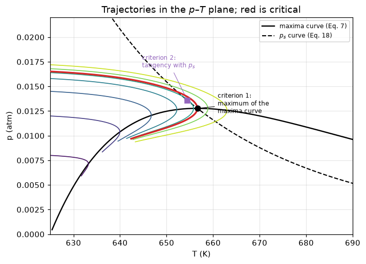
The hot spot against the inlet pressure
The profiles above stop at 0.0172 atm, just past the critical value. Followed further with pymrm.continuation, the hot spot shows what “runaway” means here: no jump and no second solution, but a stretch of inlet pressure over which it climbs by hundreds of kelvin, and beyond it a solution that is still bounded, below the adiabatic temperature \(T_w + (B/A)\,p^0\). The critical value of criterion 1 is not where that stretch is: the steepest relative sensitivity, \(\mathrm{d}\ln T_{\max}/\mathrm{d}\ln p^0\), lies about 11 % higher in inlet pressure (computed below). The criterion marks the start of the sensitive region, with a margin, not the cliff.
The curve is on the page’s 1500 cells. There the steep part is under-resolved by a few kelvin: the hot spot at 0.0182 atm is 3.1 K and at 0.019 atm 2.7 K below its value converged in the grid (Richardson from 12 000 and 24 000 cells), against 0.04 K in the controlled region (Validation).
P_SWEEP = np.round(np.arange(0.008, 0.0190 + 1e-9, 1e-4), 6)
TRACE = RunawayTube(CASE, P_SWEEP[0], TW).trace_inlet(P_SWEEP)
assert TRACE.success, TRACE.message
HS_SWEEP = np.array([x[:, 1].max() for x in TRACE.xs])


def hot_spot(p0, Tw=TW, case=CASE, **kw):
    """Hot spot (K) of an independent solve from the inlet state."""
    return RunawayTube(case, p0, Tw, **kw).solve().hot_spot()


SENS_P = (0.0164, 0.0164 * 1.05, 0.0182, 0.0182 * 1.01, 0.0190)


def hot_spots(case=CASE, n_z=1500):
    """Hot spots at SENS_P on ``n_z`` cells."""
    return np.array([hot_spot(p, case=case, n_z=n_z) for p in SENS_P])


def converged_hot_spots(case=CASE):
    """Hot spots at SENS_P, Richardson-extrapolated from 12 000 and 24 000 cells."""
    h1, h2 = hot_spots(case, 12000), hot_spots(case, 24000)
    return h2 + (h2 - h1)


def sensitivity(hs):
    """Hot-spot rise for 5 % more p0 from 0.0164 atm and for 1 % more from 0.0182 atm."""
    return hs[1] - hs[0], hs[3] - hs[2]


def steepest_over_critical_pct(hs_sweep, p_crit=None):
    """Where d ln T_max / d ln p0 is largest along the sweep, % above the critical p0."""
    slope = np.gradient(np.log(hs_sweep), np.log(P_SWEEP))
    return (P_SWEEP[int(np.argmax(slope))] / (P_CRIT if p_crit is None else p_crit) - 1) * 100


HS_1500, HS_CONV = hot_spots(), converged_hot_spots()
DT_5PCT, DT_1PCT = sensitivity(HS_1500)
DT_5PCT_CONV, DT_1PCT_CONV = sensitivity(HS_CONV)
ERR_0182, ERR_0190 = HS_CONV[2] - HS_1500[2], HS_CONV[4] - HS_1500[4]
STEEP_PCT = steepest_over_critical_pct(HS_SWEEP)
HS_019 = HS_SWEEP[-1]
T_AD_019 = TW + CASE.B / CASE.A * P_SWEEP[-1]

fig, ax = plt.subplots(figsize=(6.6, 4.3))
ax.plot(P_SWEEP * 1000, HS_SWEEP, "k-", lw=1.6, label="hot spot, pymrm continuation")
ax.plot(P_SWEEP * 1000, TW + CASE.B / CASE.A * P_SWEEP, ":", color="tab:gray",
        label=r"adiabatic limit $T_w + (B/A)\,p^0$")
ax.axvline(P_CRIT * 1000, color="tab:red", lw=1.0, ls="--", label="critical (criterion 1)")
ax.set(xlabel=r"$p^0$ (10$^{-3}$ atm)", ylabel=r"$T_{\max}$ (K)", ylim=(620, 1450),
       title=f"Hot spot against inlet pressure, $T_w$ = {TW:.0f} K")
ax.legend(fontsize=8, loc="upper left")
fig.tight_layout()
plt.show()

print(f"5 % more p0 from 0.0164 atm: hot spot +{DT_5PCT:.1f} K on 1500 cells, "
      f"+{DT_5PCT_CONV:.2f} K converged")
print(f"1 % more p0 from 0.0182 atm: hot spot +{DT_1PCT:.0f} K on 1500 cells, "
      f"+{DT_1PCT_CONV:.0f} K converged")
print(f"grid error of the hot spot on 1500 cells: {ERR_0182:.1f} K at 0.0182 atm, "
      f"{ERR_0190:.1f} K at 0.019 atm")
print(f"at p0 = {P_SWEEP[-1]:.4f} atm the hot spot is {HS_019:.0f} K on 1500 cells "
      f"({HS_CONV[4]:.0f} K converged), below the adiabatic {T_AD_019:.0f} K")
print(f"steepest d ln T_max / d ln p0 at {STEEP_PCT:.0f} % above criterion 1's critical "
      f"p0 (sampled every 1e-4 atm)")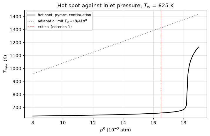
5 % more p0 from 0.0164 atm: hot spot +7.4 K on 1500 cells, +7.47 K converged
1 % more p0 from 0.0182 atm: hot spot +304 K on 1500 cells, +304 K converged
grid error of the hot spot on 1500 cells: 3.1 K at 0.0182 atm, 2.7 K at 0.019 atm
at p0 = 0.0190 atm the hot spot is 1165 K on 1500 cells (1167 K converged), below the adiabatic 1417 K
steepest d ln T_max / d ln p0 at 11 % above criterion 1's critical p0 (sampled every 1e-4 atm)
The runaway boundary across wall temperatures (their Fig. 8)
Their Fig. 8 gives the critical inlet pressure against the wall temperature: four curves (the two criteria’s brackets) through a handful of points, because each exact value cost a numerical back-integration. Here each criterion’s exact value is the same back-integration, at 21 wall temperatures, and the interesting quantity is not the boundary itself but the width of the bracket, which is the price of not integrating.
TW_SWEEP = np.arange(600.0, 701.0, 5.0)


def criteria_sweep(case=CASE, limits=inlet_limits, tangency=t_tangency):
    """Brackets, means and exact (back-integrated) inlet pressures of both criteria.

    Each criterion has its own critical trajectory and therefore its own exact
    inlet pressure; comparing both against criterion 1's would flatter one of them.
    """
    out = {k: [] for k in ("lo1", "up1", "m1", "ex1", "lo2", "up2", "m2", "ex2")}
    for T in TW_SWEEP:
        T1 = t_max_peak(case, T)
        T2 = tangency(case, T)
        for i, Tc, pc in ((1, T1, maxima_curve(case, T1, T)), (2, T2, ps_curve(case, T2))):
            lo, up, mean = limits(case, Tc, T)
            out[f"lo{i}"].append(lo)
            out[f"up{i}"].append(up)
            out[f"m{i}"].append(mean)
            out[f"ex{i}"].append(back_integrate(case, Tc, pc, T))
    s = {k: np.array(v) for k, v in out.items()}
    s["w1"] = (s["up1"] - s["lo1"]) / s["ex1"] * 100       # bracket width, % of own exact
    s["w2"] = (s["up2"] - s["lo2"]) / s["ex2"] * 100
    s["e1"] = (s["m1"] / s["ex1"] - 1) * 100                # error of the mean, %
    s["e2"] = (s["m2"] / s["ex2"] - 1) * 100
    s["cons"] = (1 - s["ex2"] / s["ex1"]) * 100             # criterion 2 below criterion 1, %
    return s


SW = criteria_sweep()
I625 = int(np.argmin(abs(TW_SWEEP - TW)))

fig, axes = plt.subplots(1, 2, figsize=(11.5, 4.4))
ax = axes[0]
ax.fill_between(TW_SWEEP, SW["lo1"], SW["up1"], color="tab:blue", alpha=0.16,
                label="criterion 1 bracket")
ax.fill_between(TW_SWEEP, SW["lo2"], SW["up2"], color="tab:purple", alpha=0.16,
                label="criterion 2 bracket")
ax.plot(TW_SWEEP, SW["m1"], color="tab:blue", lw=1.3, ls="--", label="criterion 1 mean")
ax.plot(TW_SWEEP, SW["m2"], color="tab:purple", lw=1.3, ls="--", label="criterion 2 mean")
ax.plot(TW_SWEEP, SW["ex1"], color="k", lw=2.0, label="criterion 1, exact")
ax.plot(TW_SWEEP, SW["ex2"], color="k", lw=1.2, ls="-.", label="criterion 2, exact")
ax.set(xlabel=r"$T_w$ (K)", ylabel=r"critical $p^0$ (atm)", xlim=(600, 700),
       ylim=(0, 0.045), title="Their Fig. 8, at 21 wall temperatures")
ax.legend(fontsize=8)

ax = axes[1]
ax.plot(TW_SWEEP, SW["w1"], color="tab:blue", lw=1.8, label="criterion 1, bracket width")
ax.plot(TW_SWEEP, SW["w2"], color="tab:purple", lw=1.8, label="criterion 2, bracket width")
ax.plot(TW_SWEEP, SW["e1"], color="tab:blue", lw=1.2, ls=":",
        label="criterion 1, error of the mean")
ax.plot(TW_SWEEP, SW["e2"], color="tab:purple", lw=1.2, ls=":",
        label="criterion 2, error of the mean")
ax.axhline(0.0, color="k", lw=0.8)
ax.set(xlabel=r"$T_w$ (K)", ylabel="% of that criterion's exact $p^0$",
       xlim=(600, 700), title="Bracket width, and the error of taking the mean")
ax.legend(fontsize=8)
fig.tight_layout()
plt.show()

print("bracket width, as a percentage of that criterion's own exact critical p0:")
for lbl, w in (("criterion 1", SW["w1"]), ("criterion 2", SW["w2"])):
    print(f"   {lbl}: {w.min():.1f} % to {w.max():.1f} %")
print("error of the mean, as a percentage of that criterion's own exact value:")
for lbl, e in (("criterion 1", SW["e1"]), ("criterion 2", SW["e2"])):
    print(f"   {lbl}: {e.min():+.2f} % to {e.max():+.2f} %")
print(f"criterion 2's bracket is the narrower at every wall temperature: "
      f"{bool(np.all(SW['w2'] < SW['w1']))}")
print(f"criterion 2's exact critical p0 is the lower at every wall temperature: "
      f"{bool(np.all(SW['cons'] > 0))}, by {SW['cons'][0]:.1f} % at 600 K and "
      f"{SW['cons'][-1]:.1f} % at 700 K")
print(f"criterion 1's mean is the closer to its exact value at every wall temperature: "
      f"{bool(np.all(abs(SW['e1']) < abs(SW['e2'])))}")
print(f"at Tw = 625 K: error of the mean {SW['e1'][I625]:+.2f} % (criterion 1) and "
      f"{SW['e2'][I625]:+.2f} % (criterion 2); exact values {SW['cons'][I625]:.2f} % apart")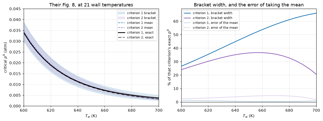
bracket width, as a percentage of that criterion's own exact critical p0:
   criterion 1: 26.5 % to 66.0 %
   criterion 2: 20.6 % to 36.7 %
error of the mean, as a percentage of that criterion's own exact value:
   criterion 1: +0.29 % to +1.21 %
   criterion 2: +1.73 % to +4.73 %
criterion 2's bracket is the narrower at every wall temperature: True
criterion 2's exact critical p0 is the lower at every wall temperature: True, by 0.3 % at 600 K and 14.8 % at 700 K
criterion 1's mean is the closer to its exact value at every wall temperature: True
at Tw = 625 K: error of the mean +0.81 % (criterion 1) and +3.16 % (criterion 2); exact values 0.93 % apart
Their Fig. 7, recomputed
Both of their Figs. 6 and 7 are graphical solutions of one implicit equation, Eq. 20, and the paper says as much: the figures are there “to facilitate the solution of (20)”. Solving it directly turns them from inputs into checks. The curve below is their Fig. 7 recomputed rather than read, and their \(t_r\) in Example 1(b) is a value they took off that graph by eye.
tr = np.linspace(19.0, 20.0, 240)


def lnK_at(t, tw):
    return np.log((t - 2.0) / (t * np.exp(-t + 20.0)) * (1.0 - t * (1.0 - t / tw)))


K_625 = CASE.A / CASE.C * np.exp(CASE.b - 20.0)
fig, ax = plt.subplots(figsize=(6.0, 4.2))
ax.plot(tr, lnK_at(tr, 20.0), "k-", lw=1.8)
ax.plot([paper("1b", "t_r")], [np.log(K_625) - (CASE.a / TW - 20.0)], "o", color="tab:red",
        ms=8, label=f"their Example 1(b):\n$t_r$ = {paper('1b', 't_r')} read off the graph")
ax.set(xlabel=r"$t_r$", ylabel=r"$\ln K_r$", xlim=(19.0, 20.0), ylim=(-5, 0),
       title="Their Fig. 7, recomputed from Eq. 20 rather than read")
ax.legend(fontsize=8, loc="lower right")
fig.tight_layout()
plt.show()

t_direct = CASE.a / CP_625["T2"]
print(f"t from solving Eq. 20 directly : {t_direct:.4f}   their graphical value "
      f"{paper('1b', 't')}")
print(f"t_r equivalent                 : {t_direct - (CASE.a / TW - 20.0):.4f}"
      f"   their {paper('1b', 't_r')}")
print(f"(T_i)_t                        : {CP_625['T2']:.2f} K   their {paper('1b', 'T_cr')} K")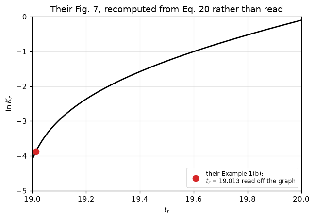
t from solving Eq. 20 directly : 20.8347   their graphical value 20.831
t_r equivalent                 : 19.0171   their 19.013
(T_i)_t                        : 654.48 K   their 654.6 K
Validation
Five checks, in increasing order of how much of the page they exercise, then the claims and the break table.
# 1. Does the parameter reading survive contact with the paper's own derived
#    quantities? Each of these depends on the whole table at once, and none was
#    used to obtain it, so a single mis-set decimal point breaks all of them.
print("1. Parameter reading, against derived values printed in the paper")
checks = [("ln K (Eq. 22)", np.log(K_625), paper("1b", "ln_K")),
          ("t_w (Eq. 21b)", CASE.a / TW, paper("1b", "t_w")),
          ("T_M (Eq. 8)", TM_625, paper("1a", "T_cr"))]
for name, val, ref in checks:
    print(f"   {name:<16} {val:>14.6g}   paper {ref:>8}   "
          f"rel {abs(val - ref) / abs(ref) * 100:5.2f} %")


def identity_gap(Tm, Tw=TW, a=CASE.a):
    """Relative gap of T_M^2 = a (T_M - T_w), which Eq. 8 makes exact."""
    return abs(Tm ** 2 - a * (Tm - Tw)) / Tm ** 2


ID_GAP = identity_gap(TM_625)
print(f"   identity T_M^2 = a(T_M - T_w), the reason Eqs. 27 and 29 agree at T_M: "
      f"relative gap below 1e-12 (here {ID_GAP:.0e})")
1. Parameter reading, against derived values printed in the paper
ln K (Eq. 22) -2.05685 paper -2.055 rel 0.09 %
t_w (Eq. 21b) 21.8176 paper 21.818 rel 0.00 %
T_M (Eq. 8) 656.618 paper 656.6 rel 0.00 %
identity T_M^2 = a(T_M - T_w), the reason Eqs. 27 and 29 agree at T_M: relative gap below 1e-12 (here 2e-15)# 2. Grid independence. First-order upwind, so successive differences halve.
GRID_NS = (200, 400, 800, 1600, 3200)
def grid_study(ns=GRID_NS, case=CASE, p0=0.0164):
"""Hot spots on the grids ``ns``, the observed order of the last three, and the
Richardson estimate of the error at the default n_z = 1500."""
vals = [hot_spot(p0, case=case, n_z=n) for n in ns]
order = np.log2((vals[-2] - vals[-3]) / (vals[-1] - vals[-2]))
richardson = vals[-1] + (vals[-1] - vals[-2])
return vals, order, abs(richardson - hot_spot(p0, case=case)), richardson
GRID_VALS, GRID_ORDER, ERR_1500, RICH = grid_study()
print("2. Grid independence: hot spot at Tw = 625 K, p0 = 0.0164 atm")
for i, (n, v) in enumerate(zip(GRID_NS, GRID_VALS)):
print(f" n_z = {n:5d} T_max = {v:.5f} K"
+ ("" if i == 0 else f" change {v - GRID_VALS[i - 1]:+.2e}"))
print(f" observed order {GRID_ORDER:.3f}; Richardson estimate {RICH:.5f} K; "
f"error at n_z = 1500 is about {ERR_1500:.1e} K")2. Grid independence: hot spot at Tw = 625 K, p0 = 0.0164 atm
n_z = 200 T_max = 655.53181 K
n_z = 400 T_max = 655.68022 K change +1.48e-01
n_z = 800 T_max = 655.75531 K change +7.51e-02
n_z = 1600 T_max = 655.79307 K change +3.78e-02
n_z = 3200 T_max = 655.81202 K change +1.89e-02
observed order 0.996; Richardson estimate 655.83096 K; error at n_z = 1500 is about 4.0e-02 K# 3. The four worked examples, one by one. `kind` separates the values that
# test the closed-form criteria from those that test the ODE solve.
def examples(case=CASE):
"""Every value printed in Section 6, recomputed for ``case``, beside the paper's."""
rows = []
def rec(example, quantity, computed):
hit = ex[(ex.example == example) & (ex.quantity == quantity)]
if hit.empty:
return
ref = float(hit.value.iloc[0])
rows.append({"example": example, "quantity": quantity, "kind": hit.kind.iloc[0],
"paper": ref, "computed": computed,
"rel_pct": abs(computed - ref) / abs(ref) * 100})
A, B, C, a, b = case.A, case.B, case.C, case.a, case.b
# Example 1(a): first criterion
TM = t_max_peak(case, TW)
lo1, up1, mean1 = inlet_limits(case, TM, TW)
cp = critical_points(case, TW)
for q, v in (("T_cr", TM), ("p0_lower", lo1), ("p0_upper", up1), ("p0_mean", mean1),
("p0_critical", cp["p0_1"])):
rec("1a", q, v)
# Example 1(b): second criterion, solving Eq. 20 instead of reading Figs. 6-7
K = A / C * np.exp(b - 20.0)
Tt = cp["T2"]
lo2, up2, mean2 = inlet_limits(case, Tt, TW)
for q, v in (("t_w", a / TW), ("ln_K", np.log(K)), ("delta_t", a / TW - 20.0),
("ln_K_r", np.log(K) - (a / TW - 20.0)), ("t", a / Tt),
("t_r", a / Tt - (a / TW - 20.0)), ("T_cr", Tt), ("p0_lower", lo2),
("p0_upper", up2), ("p0_mean", mean2), ("p0_critical", cp["p0_2"])):
rec("1b", q, v)
# Example 2: subcritical, an imposed hot spot of 640 K
Tm2 = 640.0
X2 = A / C * kexp(case, Tm2)
p_m2 = A / B * (Tm2 - TW) * (1.0 + 1.0 / np.sqrt(X2) + 1.0 / X2) # Eq. 30
rec("2", "p0_mean", p_m2)
rec("2", "p0_exact", back_integrate(case, Tm2, maxima_curve(case, Tm2, TW), TW))
rec("2", "T_max", hot_spot(p_m2, case=case))
# Example 3: given p0 and an imposed hot spot, find the wall temperature
p0_3, Tm3 = 0.0075, 675.0
dT_ad3 = B / A * p0_3 # Eq. 32
Q3 = 1.0 / np.sqrt(A / C * kexp(case, Tm3)) # Eq. 34
dT_eff3 = dT_ad3 / (1.0 + Q3 + Q3 ** 2) # Eq. 31
Tw3 = Tm3 - dT_eff3 # Eq. 33
for q, v in (("dT_ad", dT_ad3), ("Q", Q3), ("dT_eff", dT_eff3), ("T_w", Tw3),
("T_max", hot_spot(p0_3, Tw=Tw3, case=case))):
rec("3", q, v)
# Example 4: given p0 and Tw, find the radius that is critical
p0_4 = 0.0125
dT_ad4 = B / A * p0_4
dT_eff4 = TM - TW
Q4 = brentq(lambda q: 1.0 + q + q * q - dT_ad4 / dT_eff4, 0.0, 1e3)
C4 = Q4 ** 2 * A * kexp(case, TM)
for q, v in (("T_cr", TM), ("dT_eff", dT_eff4), ("dT_ad", dT_ad4), ("Q", Q4),
("C", C4), ("R", 2.0 * case.U / (case.c_p * C4))):
rec("4", q, v)
return pd.DataFrame(rows)
def example_stats(comp):
"""Mean and worst relative deviation (%), overall and per kind."""
return dict(mean=comp.rel_pct.mean(), worst=comp.rel_pct.max(),
criterion=comp[comp.kind == "criterion"].rel_pct.mean(),
integration=comp[comp.kind == "integration"].rel_pct.mean())
COMP = examples()
EXS = example_stats(COMP)
print("3. The four worked examples of Section 6\n" + COMP.to_string(index=False, formatters={
"paper": "{:.5g}".format, "computed": "{:.5g}".format, "rel_pct": "{:.3f}".format}))
for kind, sub in COMP.groupby("kind"):
print(f" {kind:<11}: n = {len(sub):2d} mean |dev| = {sub.rel_pct.mean():.3f} %"
f" worst = {sub.rel_pct.max():.3f} % ({sub.loc[sub.rel_pct.idxmax(), 'quantity']})")
print(f" overall : n = {len(COMP):2d} mean |dev| = {EXS['mean']:.3f} %"
f" worst = {EXS['worst']:.3f} %")3. The four worked examples of Section 6
example quantity kind paper computed rel_pct
1a T_cr criterion 656.6 656.62 0.003
1a p0_lower criterion 0.01353 0.013532 0.016
1a p0_upper criterion 0.01976 0.019757 0.013
1a p0_mean criterion 0.01665 0.016645 0.031
1a p0_critical integration 0.01651 0.016511 0.005
1b t_w criterion 21.818 21.818 0.002
1b ln_K criterion -2.055 -2.0568 0.090
1b delta_t criterion 1.8176 1.8176 0.000
1b ln_K_r criterion -3.873 -3.8744 0.037
1b t criterion 20.831 20.835 0.018
1b t_r criterion 19.013 19.017 0.022
1b T_cr criterion 654.6 654.48 0.018
1b p0_lower criterion 0.01423 0.014287 0.400
1b p0_upper criterion 0.01948 0.019458 0.111
1b p0_mean criterion 0.01686 0.016873 0.075
1b p0_critical integration 0.01641 0.016357 0.326
2 p0_mean criterion 0.01269 0.012684 0.044
2 p0_exact integration 0.01201 0.012011 0.007
2 T_max integration 641.5 641.52 0.003
3 dT_ad criterion 312.6 312.66 0.018
3 Q criterion 3.094 3.0931 0.030
3 dT_eff criterion 22.9 22.888 0.051
3 T_w criterion 652.2 652.11 0.014
3 T_max integration 677 676.98 0.003
4 T_cr criterion 656.6 656.62 0.003
4 dT_eff criterion 31.6 31.618 0.058
4 dT_ad criterion 521.09 521.1 0.001
4 Q criterion 3.4675 3.4662 0.037
4 C criterion 29206 29224 0.062
4 R criterion 0.0175 0.017522 0.127
criterion : n = 25 mean |dev| = 0.051 % worst = 0.400 % (p0_lower)
integration: n = 5 mean |dev| = 0.069 % worst = 0.326 % (p0_critical)
overall : n = 30 mean |dev| = 0.054 % worst = 0.400 %# 4. Two independent routes to the same critical inlet pressure. The pymrm
# reactor discretises the tube in z and its hot spot is root-found against
# T_M; the back-integration is a quadrature in the p-T plane with an adaptive
# Runge-Kutta and never forms the reactor grid at all. They should agree, and
# they are the only pair of numbers on this page that does not involve the
# paper. Bisection on the same bracket is a second route to the reactor value.
TW_CROSS = np.arange(600.0, 701.0, 20.0)
def cross_check(n_z=1500, bisect_tol=1e-7, case=CASE):
"""Per wall temperature: back-integrated and reactor critical p0, the
bracket of Eqs. 27 and 30, and the reactor value by bisection."""
rows = []
for T in TW_CROSS:
cpts = critical_points(case, T)
lo, up, mean = inlet_limits(case, cpts["T1"], T)
root = critical_p0(case, T, lo, mean, n_z=n_z)
rows.append(dict(Tw=T, back=cpts["p0_1"], reactor=root,
bisect=critical_p0_bisect(case, T, lo, mean, tol=bisect_tol, n_z=n_z),
lower=lo, upper=up))
df = pd.DataFrame(rows)
df["rel_pct"] = (df.reactor - df.back).abs() / df.back * 100
return df
CROSS = cross_check()
CROSS_WORST = CROSS.rel_pct.max()
BISECT_GAP = (CROSS.bisect - CROSS.reactor).abs().max()
BRACKETED = bool(((CROSS.lower <= CROSS.back) & (CROSS.back <= CROSS.upper)).all())
P_CRIT_REL_MARGIN = float(np.minimum((CROSS.back - CROSS.lower) / CROSS.back,
(CROSS.upper - CROSS.back) / CROSS.back).min())
print("4. pymrm reactor root vs phase-plane back-integration (criterion 1)")
for r in CROSS.itertuples():
print(f" Tw = {r.Tw:.0f} K: back-integration {r.back:.5f} pymrm {r.reactor:.5f} "
f"{r.rel_pct:5.2f} % inside its bracket: {r.lower <= r.back <= r.upper}")
print(f" worst disagreement between the two methods: {CROSS_WORST:.2f} %")
print(f" criterion 1 brackets its own critical value everywhere: {BRACKETED}")
print(f" bisection to 1e-7 atm against the root: below 1e-7 atm "
f"(here {BISECT_GAP:.0e} atm)")4. pymrm reactor root vs phase-plane back-integration (criterion 1)
Tw = 600 K: back-integration 0.03395 pymrm 0.03396 0.02 % inside its bracket: True
Tw = 620 K: back-integration 0.01890 pymrm 0.01891 0.03 % inside its bracket: True
Tw = 640 K: back-integration 0.01131 pymrm 0.01132 0.05 % inside its bracket: True
Tw = 660 K: back-integration 0.00727 pymrm 0.00728 0.08 % inside its bracket: True
Tw = 680 K: back-integration 0.00502 pymrm 0.00503 0.13 % inside its bracket: True
Tw = 700 K: back-integration 0.00371 pymrm 0.00372 0.18 % inside its bracket: True
worst disagreement between the two methods: 0.18 %
criterion 1 brackets its own critical value everywhere: True
bisection to 1e-7 atm against the root: below 1e-7 atm (here 3e-08 atm)# 5. The continuation sweep against independent solves from the inlet state.
def trace_gap(trace=TRACE, n_z=1500):
"""Largest temperature gap (K), over every cell and every traced point,
between the sweep and independent solves from the inlet state."""
return max(float(np.max(abs(x[:, 1] - RunawayTube(CASE, p, TW, n_z=n_z).solve().T)))
for p, x in zip(trace.params, trace.xs))
TRACE_GAP = trace_gap()
print(f"5. Continuation against independent solves at all {len(P_SWEEP)} inlet pressures")
print(f" largest temperature gap over all cells below 1e-6 K (here {TRACE_GAP:.0e} K)")5. Continuation against independent solves at all 111 inlet pressures
largest temperature gap over all cells below 1e-6 K (here 4e-09 K)Claims: what each number is, and how it is checked
Every number the page stands behind is registered once, in the cell below (docs/claims-design.md in the gallery repository):
- a value is a result whose size is set by physics, the data or the discretisation. CI holds it to a relative tolerance of the committed baseline, 5 % unless the cell says otherwise. Closed-form and root-found values carry tighter tolerances, set by their solver tolerances;
- a bound is a quantity whose size is not physics: an identity, a solver-tolerance gap, a convergence order. It is checked against its stated limits on every run and states its basis;
- an exact result is a count or a label, with its distance to the threshold that decided it.
# --- the worked examples ------------------------------------------------------
claims.value("examples_mean_dev_pct", EXS["mean"])
claims.value("examples_worst_dev_pct", EXS["worst"])
claims.value("criterion_mean_dev_pct", EXS["criterion"])
claims.value("integration_mean_dev_pct", EXS["integration"])
for name, n in (("n_examples", len(COMP)),
                ("n_examples_criterion", int((COMP.kind == "criterion").sum())),
                ("n_examples_integration", int((COMP.kind == "integration").sum()))):
    claims.exact(name, n, structural=True,
                 note="rows of the examples CSV that the page recomputes; set by the data")
# --- criterion 1 at 625 K ---------------------------------------------------------
claims.value("T_M_at_625K", TM_625, rtol=1e-9, unit="K")
claims.bound("tm_identity_rel", ID_GAP, max=1e-12, basis="identity",
             note="T_M^2 = a (T_M - T_w) follows from Eq. 8")
claims.value("p0_critical_at_625K", CP_625["p0_1"], rtol=1e-6, unit="atm",
             note="back-integration, solve_ivp rtol 1e-11")
claims.value("p0_critical_reactor_625K", P_CRIT, rtol=1e-6, unit="atm",
             note="brentq to 1e-12 atm on Newton solves at tol 1e-10 (scaled)")
# --- two routes, and the bisection ---------------------------------------------------
claims.value("cross_method_worst_pct", CROSS_WORST)
claims.bound("bisection_vs_root_atm", BISECT_GAP, max=1e-7, basis="tolerance",
             unit="atm", note="bisection to a bracket narrower than 1e-7 atm")
claims.exact("criterion1_brackets_exact", BRACKETED, margin=P_CRIT_REL_MARGIN,
             min_margin=0.01,
             note="margin: smallest distance of the exact value to an end of its bracket, "
                  "relative to the exact value")
# --- the grid ----------------------------------------------------------------------------
claims.bound("hotspot_grid_order", GRID_ORDER, min=0.9, max=1.1, basis="theory",
             note="first-order upwind, n_z 800, 1600, 3200")
claims.value("hotspot_error_n1500_K", ERR_1500, unit="K",
             note="Richardson estimate from n_z = 1600 and 3200")
# --- sensitivity and the continuation sweep ---------------------------------------------
claims.value("dT_hotspot_5pct_from_0164_K", DT_5PCT, unit="K", note="1500 cells")
claims.value("dT_hotspot_5pct_converged_K", DT_5PCT_CONV, unit="K",
             note="Richardson from 12000 and 24000 cells")
claims.value("dT_hotspot_1pct_converged_K", DT_1PCT_CONV, unit="K",
             note="Richardson from 12000 and 24000 cells")
claims.value("hotspot_grid_err_0182_K", ERR_0182, unit="K", note="1500 cells against converged")
claims.value("hotspot_grid_err_0190_K", ERR_0190, unit="K", note="1500 cells against converged")
claims.value("hotspot_0190_converged_K", HS_CONV[4], unit="K")
claims.value("steepest_sensitivity_above_crit_pct", STEEP_PCT, rtol=0.1,
             note="argmax on the 1e-4 atm sweep: rtol covers one sample spacing")
claims.value("dT_hotspot_1pct_from_0182_K", DT_1PCT, unit="K")
claims.value("hotspot_p0190_K", HS_019, unit="K")
claims.bound("trace_vs_independent_K", TRACE_GAP, max=1e-6, basis="tolerance", unit="K",
             note="newton tol 1e-10 on the scaled unknowns in both")
# --- the Fig. 8 sweep --------------------------------------------------------------------
claims.value("bracket_width_c1_min_pct", SW["w1"].min())
claims.value("bracket_width_c1_max_pct", SW["w1"].max())
claims.value("bracket_width_c2_min_pct", SW["w2"].min())
claims.value("bracket_width_c2_max_pct", SW["w2"].max())
claims.value("mean_error_c1_min_pct", SW["e1"].min())
claims.value("mean_error_c1_max_pct", SW["e1"].max())
claims.value("mean_error_c2_min_pct", SW["e2"].min())
claims.value("mean_error_c2_max_pct", SW["e2"].max())
claims.value("c2_below_c1_600K_pct", SW["cons"][0])
claims.value("c2_below_c1_700K_pct", SW["cons"][-1])
claims.value("mean_error_c1_625K_pct", SW["e1"][I625])
claims.value("mean_error_c2_625K_pct", SW["e2"][I625])
claims.value("c2_below_c1_625K_pct", SW["cons"][I625])
claims.exact("c2_bracket_narrower_everywhere", bool(np.all(SW["w2"] < SW["w1"])),
             margin=float((SW["w1"] - SW["w2"]).min()), min_margin=0.5,
             note="margin in percentage points of the criterion's own exact p0")
claims.exact("c2_more_conservative_everywhere", bool(np.all(SW["cons"] > 0)),
             margin=float(SW["cons"].min()), min_margin=0.05, note="margin in percent")
claims.exact("c1_mean_closer_everywhere", bool(np.all(abs(SW["e1"]) < abs(SW["e2"]))),
             margin=float((abs(SW["e2"]) - abs(SW["e1"])).min()), min_margin=0.1,
             note="margin in percentage points")

# prose numbers
claims.says("7.4", "dT_hotspot_5pct_from_0164_K")      # Background
claims.says("7.47", "dT_hotspot_5pct_converged_K")
claims.says("304", "dT_hotspot_1pct_converged_K")
claims.says("11", "steepest_sensitivity_above_crit_pct")  # "about 11 % higher"
claims.says("3.1", "hotspot_grid_err_0182_K")
claims.says("2.7", "hotspot_grid_err_0190_K")
claims.says("304", "dT_hotspot_1pct_from_0182_K")      # Background
claims.says("27", "bracket_width_c1_min_pct")          # What pymrm adds: "27 % to 66 %"
claims.says("66", "bracket_width_c1_max_pct")
claims.says("21", "bracket_width_c2_min_pct")          # "21 % to 37 %"
claims.says("37", "bracket_width_c2_max_pct")
claims.says("0.3", "c2_below_c1_600K_pct")             # "0.3 % at 600 K"
claims.says("15", "c2_below_c1_700K_pct")              # "15 % at 700 K"
claims.says("0.3", "mean_error_c1_min_pct")            # "+0.3 % to +1.2 %"
claims.says("1.2", "mean_error_c1_max_pct")
claims.says("1.7", "mean_error_c2_min_pct")            # "+1.7 % to +4.7 %"
claims.says("4.7", "mean_error_c2_max_pct")
claims.says("0.8", "mean_error_c1_625K_pct")           # "0.8 % ... 3.2 %"
claims.says("3.2", "mean_error_c2_625K_pct")
claims.says("0.9", "c2_below_c1_625K_pct")             # "differ by 0.9 %"
claims.says("0.18", "cross_method_worst_pct") # What pymrm addsTrueThe defect-injection table
Each row breaks one thing on purpose, re-runs the computation behind one claim with the defect in place, and hands the result to claims.breaks, which records whether the claim’s own check (its tolerance or its bound) catches it. The first row is the units trap of this paper. Every claim that is not structural must be failed by at least one row, and the last cell of the page raises otherwise.
BREAK = []


def brk(name, metric, value, note=""):
    """One injected defect: ``value`` is what claim ``metric`` becomes with it."""
    caught = claims.breaks(name, metric, value)
    clean = claims[metric]
    if claims.metrics[metric]["kind"] == "bound":
        clean = f"(here {clean:.2e})"      # a bound's own value is not published: masked
    BREAK.append(dict(defect=name, metric=metric, clean=clean, broken=value,
                      caught=caught, note=note))


# --- the units trap: c_p multiplied by rho_g ------------------------------------------
TRAP = "c_p multiplied by rho_g (the units trap)"
CASE_TRAP = replace(CASE, c_p=CASE.c_p * CASE.rho_g)
_exs = example_stats(examples(CASE_TRAP))
for k, metric in (("mean", "examples_mean_dev_pct"), ("worst", "examples_worst_dev_pct"),
                  ("criterion", "criterion_mean_dev_pct"),
                  ("integration", "integration_mean_dev_pct")):
    brk(TRAP, metric, _exs[k])
brk(TRAP, "p0_critical_at_625K", critical_points(CASE_TRAP, TW)["p0_1"])
_lo, _up, _mean = inlet_limits(CASE_TRAP, TM_625, TW)
brk(TRAP, "p0_critical_reactor_625K", critical_p0(CASE_TRAP, TW, _lo, _mean))
_hs_trap, _hs_conv_trap = hot_spots(CASE_TRAP), converged_hot_spots(CASE_TRAP)
_dt5, _dt1 = sensitivity(_hs_trap)
brk(TRAP, "dT_hotspot_5pct_from_0164_K", _dt5)
brk(TRAP, "dT_hotspot_1pct_from_0182_K", _dt1)
_dt5c, _dt1c = sensitivity(_hs_conv_trap)
brk(TRAP, "dT_hotspot_5pct_converged_K", _dt5c)
brk(TRAP, "dT_hotspot_1pct_converged_K", _dt1c)
brk(TRAP, "hotspot_grid_err_0182_K", _hs_conv_trap[2] - _hs_trap[2])
brk(TRAP, "hotspot_grid_err_0190_K", _hs_conv_trap[4] - _hs_trap[4])
brk(TRAP, "hotspot_0190_converged_K", _hs_conv_trap[4])
brk(TRAP, "hotspot_error_n1500_K", grid_study(case=CASE_TRAP)[2])
_sw_trap = criteria_sweep(CASE_TRAP)
for metric, val in (("c2_below_c1_600K_pct", _sw_trap["cons"][0]),
                    ("c2_below_c1_700K_pct", _sw_trap["cons"][-1]),
                    ("mean_error_c1_625K_pct", _sw_trap["e1"][I625]),
                    ("mean_error_c2_625K_pct", _sw_trap["e2"][I625]),
                    ("c2_below_c1_625K_pct", _sw_trap["cons"][I625]),
                    ("bracket_width_c1_min_pct", _sw_trap["w1"].min()),
                    ("bracket_width_c2_min_pct", _sw_trap["w2"].min()),
                    ("mean_error_c2_min_pct", _sw_trap["e2"].min()),
                    ("c1_mean_closer_everywhere",
                     bool(np.all(abs(_sw_trap["e1"]) < abs(_sw_trap["e2"]))))):
    brk(TRAP, metric, val)
_trace_trap = RunawayTube(CASE_TRAP, P_SWEEP[0], TW).trace_inlet(P_SWEEP)
assert _trace_trap.success, _trace_trap.message
brk(TRAP, "hotspot_p0190_K", _trace_trap.xs[-1][:, 1].max())
brk("critical p0 taken as the Eq. 28 upper limit", "steepest_sensitivity_above_crit_pct",
    steepest_over_critical_pct(HS_SWEEP, UP_625))


# --- the criteria ------------------------------------------------------------------------
def _t_max_peak_plus(case, Tw):
    """Eq. 8 with the other root of the quadratic."""
    return 0.5 * (case.a + np.sqrt(case.a * (case.a - 4.0 * Tw)))


def _t_max_peak_typo(case, Tw):
    """Eq. 8 with 2 T_w instead of 4 T_w under the root."""
    return 0.5 * (case.a - np.sqrt(case.a * (case.a - 2.0 * Tw)))


brk("Eq. 8 with the other root of the quadratic", "T_M_at_625K", _t_max_peak_plus(CASE, TW))
brk("Eq. 8 with 2 T_w under the root", "tm_identity_rel",
    identity_gap(_t_max_peak_typo(CASE, TW)))


def _limits_no_square(case, T_cr, Tw, T0=None):
    """Eq. 28 without the square."""
    lo, _, _ = inlet_limits(case, T_cr, Tw, T0)
    X = case.A / case.C * kexp(case, T_cr)
    up = case.A / case.B * (T_cr - Tw) * (1.0 / np.sqrt(X) + 1.0)
    return lo, up, 0.5 * (lo + up)


NOSQ = "Eq. 28 without the square"
_sw_nosq = criteria_sweep(limits=_limits_no_square)
for metric, val in (("bracket_width_c1_max_pct", _sw_nosq["w1"].max()),
                    ("bracket_width_c2_max_pct", _sw_nosq["w2"].max()),
                    ("mean_error_c1_min_pct", _sw_nosq["e1"].min()),
                    ("mean_error_c1_max_pct", _sw_nosq["e1"].max()),
                    ("mean_error_c2_max_pct", _sw_nosq["e2"].max()),
                    ("c1_mean_closer_everywhere",
                     bool(np.all(abs(_sw_nosq["e1"]) < abs(_sw_nosq["e2"]))))):
    brk(NOSQ, metric, val)
_cross_nosq = [_limits_no_square(CASE, t_max_peak(CASE, T), T) for T in TW_CROSS]
_cross_nosq = [lo <= b <= up for (lo, up, _), b in zip(_cross_nosq, CROSS.back)]
brk(NOSQ, "criterion1_brackets_exact", bool(all(_cross_nosq)))
TWTM = "Eq. 20 with t_w = a/T_M instead of a/T_w"
_sw_twtm = criteria_sweep(tangency=lambda case, Tw: t_tangency(case, t_max_peak(case, Tw)))
brk(TWTM, "c2_bracket_narrower_everywhere", bool(np.all(_sw_twtm["w2"] < _sw_twtm["w1"])))
brk(TWTM, "c2_more_conservative_everywhere", bool(np.all(_sw_twtm["cons"] > 0)))

# --- discretisation and solvers ---------------------------------------------------------------
brk("reactor on n_z = 1000", "cross_method_worst_pct", cross_check(n_z=1000).rel_pct.max())
brk("reactor on n_z = 1000", "p0_critical_reactor_625K",
    critical_p0(CASE, TW, LO_625, MEAN_625, n_z=1000))
brk("bisection to 1e-4 atm", "bisection_vs_root_atm",
    abs(critical_p0_bisect(CASE, TW, LO_625, MEAN_625, tol=1e-4) - P_CRIT))
brk("last grid 2400 cells, read as a doubling", "hotspot_grid_order",
    grid_study(ns=(200, 400, 800, 1600, 2400))[1])
_trace_1000 = RunawayTube(CASE, P_SWEEP[0], TW, n_z=1000).trace_inlet(P_SWEEP)
brk("sweep on n_z = 1000, independent solves on 1500", "trace_vs_independent_K",
    max(abs(x[:, 1].max() - h) for x, h in zip(_trace_1000.xs, HS_SWEEP)))

pd.set_option("display.width", 200)
print(pd.DataFrame(BREAK).to_string(index=False, formatters={
    "clean": lambda v: f"{v:.5g}" if isinstance(v, float) else str(v),
    "broken": lambda v: f"{v:.5g}" if isinstance(v, float) else str(v)}))
defect metric clean broken caught note
c_p multiplied by rho_g (the units trap) examples_mean_dev_pct 0.054104 5.5103 True
c_p multiplied by rho_g (the units trap) examples_worst_dev_pct 0.40029 26.855 True
c_p multiplied by rho_g (the units trap) criterion_mean_dev_pct 0.05118 6.2057 True
c_p multiplied by rho_g (the units trap) integration_mean_dev_pct 0.068722 2.0335 True
c_p multiplied by rho_g (the units trap) p0_critical_at_625K 0.016511 0.017177 True
c_p multiplied by rho_g (the units trap) p0_critical_reactor_625K 0.016517 0.017183 True
c_p multiplied by rho_g (the units trap) dT_hotspot_5pct_from_0164_K 7.4338 4.5799 True
c_p multiplied by rho_g (the units trap) dT_hotspot_1pct_from_0182_K 304.42 2.4442 True
c_p multiplied by rho_g (the units trap) dT_hotspot_5pct_converged_K 7.4667 4.5914 True
c_p multiplied by rho_g (the units trap) dT_hotspot_1pct_converged_K 303.7 2.4575 True
c_p multiplied by rho_g (the units trap) hotspot_grid_err_0182_K 3.058 0.071838 True
c_p multiplied by rho_g (the units trap) hotspot_grid_err_0190_K 2.6616 0.22021 True
c_p multiplied by rho_g (the units trap) hotspot_0190_converged_K 1167.3 682.83 True
c_p multiplied by rho_g (the units trap) hotspot_error_n1500_K 0.040405 0.026517 True
c_p multiplied by rho_g (the units trap) c2_below_c1_600K_pct 0.28099 0.39456 True
c_p multiplied by rho_g (the units trap) c2_below_c1_700K_pct 14.831 18.982 True
c_p multiplied by rho_g (the units trap) mean_error_c1_625K_pct 0.81138 0.67926 True
c_p multiplied by rho_g (the units trap) mean_error_c2_625K_pct 3.1554 3.4699 True
c_p multiplied by rho_g (the units trap) c2_below_c1_625K_pct 0.93427 1.2992 True
c_p multiplied by rho_g (the units trap) bracket_width_c1_min_pct 26.539 29.447 True
c_p multiplied by rho_g (the units trap) bracket_width_c2_min_pct 20.553 11.248 True
c_p multiplied by rho_g (the units trap) mean_error_c2_min_pct 1.7281 -1.1006 True
c_p multiplied by rho_g (the units trap) c1_mean_closer_everywhere True False True
c_p multiplied by rho_g (the units trap) hotspot_p0190_K 1164.7 682.61 True
critical p0 taken as the Eq. 28 upper limit steepest_sensitivity_above_crit_pct 10.797 -7.3766 True
Eq. 8 with the other root of the quadratic T_M_at_625K 656.62 12979 True
Eq. 8 with 2 T_w under the root tm_identity_rel (here 2.43e-15) 41.611 True
Eq. 28 without the square bracket_width_c1_max_pct 65.965 -8.935 True
Eq. 28 without the square bracket_width_c2_max_pct 36.666 -47.315 True
Eq. 28 without the square mean_error_c1_min_pct 0.29351 -48.372 True
Eq. 28 without the square mean_error_c1_max_pct 1.2069 -36.598 True
Eq. 28 without the square mean_error_c2_max_pct 4.7298 -32.809 True
Eq. 28 without the square c1_mean_closer_everywhere True False True
Eq. 28 without the square criterion1_brackets_exact True False True
Eq. 20 with t_w = a/T_M instead of a/T_w c2_bracket_narrower_everywhere True False True
Eq. 20 with t_w = a/T_M instead of a/T_w c2_more_conservative_everywhere True False True
reactor on n_z = 1000 cross_method_worst_pct 0.18252 0.27374 True
reactor on n_z = 1000 p0_critical_reactor_625K 0.016517 0.01652 True
bisection to 1e-4 atm bisection_vs_root_atm (here 2.99e-08) 1.7838e-05 True
last grid 2400 cells, read as a doubling hotspot_grid_order (here 9.96e-01) 1.5811 True
sweep on n_z = 1000, independent solves on 1500 trace_vs_independent_K (here 4.16e-09) 1.6793 True What pymrm adds
Their Figs. 6 and 7 exist only because there was no computer. Both are graphical solutions of Eq. 20. Solving it directly (t_tangency) turns them from inputs into checks, and the recomputed Fig. 7 above shows where their graphical reading sits.
Their Fig. 8 was four curves through a handful of points. Each exact value on it cost a numerical back-integration, so the paper computed few. With the same back-integration at 21 wall temperatures, three things the original could only assert at a point are visible across the range.
The bracket is wide: 27 % to 66 % of the value it brackets for the first criterion, 21 % to 37 % for the second. So the useful output of the method was never the bracket itself but its midpoint. That is what makes the “rather curious rule” the authors report worth reporting.
The second criterion’s bracket really is the narrower, at every wall temperature, as they claim, and its critical pressure really is the more conservative: lower than the first criterion’s at every wall temperature, by 0.3 % at 600 K and 15 % at 700 K.
But the first criterion’s midpoint is the better estimate, not the second’s, at every wall temperature: +0.3 % to +1.2 % against its own exact value, where the second criterion’s midpoint runs +1.7 % to +4.7 % high. The paper compares the two only at \(T_w\) = 625 K, where their exact critical pressures differ by 0.9 %, and concludes they “entirely confirm” each other. Already there the first criterion’s midpoint is 0.8 % above its exact value and the second’s 3.2 %: narrower bracket and better midpoint are different virtues, and here they belong to different criteria.
The pymrm reactor is the independent check. The exact values above come from the phase plane; the reactor model solves the tube itself, and its hot spot reaches \(T_M\) at inlet pressures that agree with the back-integration to 0.18 % or better from 600 to 700 K, the first-order upwind error at 1500 cells. The same model, followed with pymrm.continuation, draws the hot spot through the runaway region, where the solution stays bounded and every continuation step converges.
That is the honest limit of this page. Nothing here contradicts the paper: the criteria are reproduced, not improved, but it does quantify, across the operating plane, claims the original supports at a single point.
Reuse
The criteria on their own. t_max_peak, t_tangency and inlet_limits in model.py need only a VWFCase (the groups \(A\), \(B\), \(C\) and the Arrhenius constants \(a\), \(b\)): no reactor object, no pymrm. For a different chemistry, build a VWFCase from its constants and the criteria carry over unchanged, provided the reaction is still pseudo-first-order and irreversible.
The reactor. RunawayTube.residual is the whole model, and RunawayTube.set_inlet changes the inlet without rebuilding an operator. To add axial dispersion, build a construct_grad/construct_div diffusion operator and add it to jac_const, and replace the inlet dictionary by a Danckwerts condition ({"a": D, "b": v, "d": v} with the inlet values through shapes_d): the source term does not change. To make the wall temperature vary along the tube, give Tw as an array of shape (n_z,); reaction broadcasts it. To move to a two-phase (heterogeneous) description, the pellet equation of B1.1 couples in through pymrm.coupling.BlockLayout.
Thresholds. critical_p0 finds the inlet pressure at which the hot spot reaches any target, by a root-finder on independent solves. Give it a lower end below the root and a first guess of the upper end (the paper’s Eq. 27 and Eq. 30 values for the first criterion); it raises the upper end by 1 % at a time until the root is bracketed, and raises a ValueError after 30 tries. Keep the guess close: far above the critical value, Newton from the inlet state does not converge. trace_inlet follows the hot spot over a list of inlet pressures with pymrm.continuation.
Watch the units. \(c_p\) is volumetric here. If you take \(c_p\) from a data book in kcal/(kg·°C), multiply by \(\rho_g\) before using it in \(B\) and \(C\).
Related pages. C2.1 (the same plug-flow operators, real kinetics), B1.1 (multiplicity, which this problem does not have), C2.10 (o-xylene, the classic hot spot, the same reactor three years earlier), D2.1, D2.3.
Cite the source, not this page: Van Welsenaere, R. J. and Froment, G. F., Parametric sensitivity and runaway in fixed bed catalytic reactors, Chemical Engineering Science 25(10) 1503–1516 (1970), doi:10.1016/0009-2509(70)85073-4.
# Claims: prints every registered number, writes agreement.json for CI, and
# raises when a claim fails its own check or has no break row.
claims.report();   # the semicolon keeps the notebook from echoing the payload
Claims for D2.2:
examples_mean_dev_pct = 0.054104 value rtol 0.05
examples_worst_dev_pct = 0.40029 value rtol 0.05
criterion_mean_dev_pct = 0.05118 value rtol 0.05
integration_mean_dev_pct = 0.068722 value rtol 0.05
n_examples = 30 exact exact
n_examples_criterion = 25 exact exact
n_examples_integration = 5 exact exact
T_M_at_625K = 656.62 value rtol 1e-09
tm_identity_rel = (here 2.4e-15) bound bound <= 1e-12 [identity]
p0_critical_at_625K = 0.016511 value rtol 1e-06
p0_critical_reactor_625K = 0.016517 value rtol 1e-06
cross_method_worst_pct = 0.18252 value rtol 0.05
bisection_vs_root_atm = (here 3.0e-08) bound bound <= 1e-07 [tolerance]
criterion1_brackets_exact = True exact exact, margin 0.121
hotspot_grid_order = (here 1.0e+00) bound bound [0.9, 1.1] [theory]
hotspot_error_n1500_K = 0.040405 value rtol 0.05
dT_hotspot_5pct_from_0164_K = 7.4338 value rtol 0.05
dT_hotspot_5pct_converged_K = 7.4667 value rtol 0.05
dT_hotspot_1pct_converged_K = 303.7 value rtol 0.05
hotspot_grid_err_0182_K = 3.058 value rtol 0.05
hotspot_grid_err_0190_K = 2.6616 value rtol 0.05
hotspot_0190_converged_K = 1167.3 value rtol 0.05
steepest_sensitivity_above_crit_pct = 10.797 value rtol 0.1
dT_hotspot_1pct_from_0182_K = 304.42 value rtol 0.05
hotspot_p0190_K = 1164.7 value rtol 0.05
trace_vs_independent_K = (here 4.2e-09) bound bound <= 1e-06 [tolerance]
bracket_width_c1_min_pct = 26.539 value rtol 0.05
bracket_width_c1_max_pct = 65.965 value rtol 0.05
bracket_width_c2_min_pct = 20.553 value rtol 0.05
bracket_width_c2_max_pct = 36.666 value rtol 0.05
mean_error_c1_min_pct = 0.29351 value rtol 0.05
mean_error_c1_max_pct = 1.2069 value rtol 0.05
mean_error_c2_min_pct = 1.7281 value rtol 0.05
mean_error_c2_max_pct = 4.7298 value rtol 0.05
c2_below_c1_600K_pct = 0.28099 value rtol 0.05
c2_below_c1_700K_pct = 14.831 value rtol 0.05
mean_error_c1_625K_pct = 0.81138 value rtol 0.05
mean_error_c2_625K_pct = 3.1554 value rtol 0.05
c2_below_c1_625K_pct = 0.93427 value rtol 0.05
c2_bracket_narrower_everywhere = True exact exact, margin 2.57
c2_more_conservative_everywhere = True exact exact, margin 0.281
c1_mean_closer_everywhere = True exact exact, margin 0.876