# Bootstrap: the pymrm this page was checked with, and the gallery files it was
# published with. Works in a checkout, in CI and on a fresh Colab VM.
GALLERY_REF = "gallery-2026.11.10.3"  # replaced by the release tag at publication
PYMRM = ">=3.3.0,<4"  # equals meta.yaml pymrm_min_version, up to the next major
PAGE = "A2.5-edwards-richardson-dispersion"  # equals the page directory

import os, sys, urllib.request
from pathlib import Path
_shared = next((p / "shared" for p in (Path.cwd(), *Path.cwd().parents)
                if (p / "shared" / "gallery_bootstrap.py").is_file()), None)
if _shared is None:
    _shared = (Path(os.environ.get("XDG_CACHE_HOME") or Path.home() / ".cache")
               / "pymrm-gallery" / GALLERY_REF)
    _shared.mkdir(parents=True, exist_ok=True)
    urllib.request.urlretrieve(
        "https://raw.githubusercontent.com/computational-chemical-engineering/"
        f"pymrm-gallery/{GALLERY_REF}/shared/gallery_bootstrap.py",
        _shared / "gallery_bootstrap.py")
sys.path.insert(0, str(_shared))
sys.modules.pop("gallery_bootstrap", None)
from gallery_bootstrap import setup
setup(PAGE, PYMRM, GALLERY_REF); # the semicolon stops the cell echoing the pathWhere the axial dispersion coefficient comes from: Edwards & Richardson’s packed bed
sec:A
struct:S4
tier:T1
data:tier2
phase:gas
A pulse of argon in air, two response curves, and the two-point moment method that turns them into D_L, reproduced in pymrm, against the points digitised from their Figure 9.
Where the axial dispersion coefficient comes from
Catalog ID: A2.5 · Structures: S4 (1-D transient advection-dispersion) · Tier: T1
A2.1 takes the axial-dispersion reactor as given and asks what its boundary conditions mean. A2.3 derives a dispersion coefficient for a tube from first principles. This page is about the third question, the experimental one: for a real packed bed, where does the number come from, and how good is it?
import time
import numpy as np
import pandas as pd
import matplotlib.pyplot as plt
from IPython.display import Markdown, display
from scipy.optimize import least_squares
from pymrm import vanleer
from gallery_utils import load_data, load_meta, cite_data, Claims
from model import (TracerBed, simulate_experiment, simulate_two_zone,  # this page's model.py
                   moments, invert_two_point, emg, D_two_zone, channelling_case,
                   two_zone_split, peak_time, STEP_LOG, X0, X1, SIGMA, TAIL)

plt.rcParams.update({"figure.dpi": 110, "axes.grid": True, "grid.alpha": 0.3})
claims = Claims(PAGE.split("-")[0])
SEED = 20260802                # every resampling below seeds from this, explicitly


# Deviations are reported ONE way everywhere on this page:
#     dev = (model - measured) / measured
def dev(model, measured):
    return np.asarray(model, float) / np.asarray(measured, float) - 1.0
Background
Edwards and Richardson pushed air through beds of glass ballotini, sand and powdered perspex, injected a pulse of argon, and watched it come out on a \(\beta\)-ray ionisation detector. They did this over a wider Reynolds-number range than anyone before them (the range they print is listed under Parameters and assumptions) and produced the correlation that is still quoted for gas-phase axial dispersion in packed beds.
Three things make this a page rather than a curve fit.
The measurement is an inverse problem, and its forward model is the thing the gallery already builds. A dispersion coefficient is never observed. What is observed is a concentration against time at two positions; \(D_L\) is whatever value of the parameter in
\[\frac{\partial c}{\partial t} + u\frac{\partial c}{\partial x} = D_L\frac{\partial^2 c}{\partial x^2}\]
makes the second curve follow from the first. So a page that can solve that equation can simulate the whole experiment, invert it with the authors’ own formulae, and check that the number it gets back is the number it put in. That check has real power, because the discretisation adds dispersion of its own and the inversion cannot tell it apart from the physical kind.
The correlation has structure, not just constants. It is a molecular diffusion floor plus an eddy-diffusion term, and each has a limit the model must hit: at low Reynolds number \(D_L\) must approach the molecular diffusivity times a tortuosity factor, and at high Reynolds number the Péclet number must approach 2. In between, the data show a maximum in Péclet number that the sum of those two mechanisms cannot produce at all, and that is what the paper’s third term is for.
They also found where their own model fails. With their finest particles the moment analysis returned dispersion coefficients far above the correlation, and the response curve computed from the fitted \(D_L\) peaked later than the one they measured. They attributed it to channelling. That diagnostic, the shape disagreeing while the moments agree by construction, is reproduced in the last part of the results.
The published model
The measurement
For a pulse in an infinite uniform bed, Aris showed that two response curves measured a distance \(\Delta x\) apart are related by three exact statements, which are Edwards & Richardson’s Eqs. (5), (6) and (7):
\[A_1 = A_2, \qquad \Delta\bar t = \bar t_2 - \bar t_1 = \frac{\Delta x}{u}, \qquad \Delta\sigma^2 = \sigma_2^2 - \sigma_1^2 = \frac{2 D_L \Delta x}{u^3},\]
with area, mean and variance defined by their Eqs. (2) to (4),
\[A=\int_0^\infty c\,\mathrm dt,\qquad \bar t=\frac1A\int_0^\infty c\,t\,\mathrm dt,\qquad \sigma^2=\frac1A\int_0^\infty c\,t^2\,\mathrm dt-\bar t^{\,2}.\]
Everything that happens before the first detector (the shape of the injected pulse, the distributor, the entrance section) cancels in the differences. That is the whole point of measuring twice, and it is why the method needs no knowledge of the input.
The three relations are exact for the equation above, not approximations. In Laplace space the downstream transfer function is \(\exp(\lambda\Delta x)\) with \(\lambda = \bigl(u-\sqrt{u^2+4D_Ls}\bigr)/2D_L = -s/u + D_Ls^2/u^3 + O(s^3)\), and the first three coefficients of that expansion are exactly the three statements above.
The correlation
Two mechanisms, taken as additive (their Eqs. 13 to 15):
\[D_L = \gamma D_M + \tfrac12 u d_p .\]
The first term is molecular diffusion reduced by the tortuosity of the bed; the second is the mixing-cell and turbulent-mixing limit \(\mathrm{Pe} = u d_p/D_L = 2\) of Aris & Amundson and of Prausnitz. This form rises monotonically to \(\mathrm{Pe}=2\) and can never exceed it, but the measurements do. Radial mixing inside the bed reduces axial spreading, and E&R put that in as an empirical correction factor on the eddy term (their Eq. 16):
\[D_L = \gamma D_M + \frac{\tfrac12 u d_p}{1 + \beta D_M/(u d_p)} .\]
With \(\gamma\) measured and \(\beta\) fitted this is their Eq. (17), quoted in the abstract as the result of the paper, and divided through by \(u d_p\) with the voidage \(\varepsilon\) and Schmidt number \(\mathrm{Sc}\) they state, their Eq. (18):
\[\mathrm{Pe}^{-1} = \frac{a}{\mathrm{Re}} + \frac{\tfrac12}{1+b/\mathrm{Re}}, \qquad a = \frac{\gamma\varepsilon}{\mathrm{Sc}},\quad b = \frac{\beta\varepsilon}{\mathrm{Sc}} .\]
The constants as printed are listed in the next cell, read from the dataset.
Definitions matter here. \(u\) is the interstitial velocity throughout, so \(\mathrm{Re} = u d_p \varepsilon/\nu\) is built on the superficial velocity \(u\varepsilon\) while \(\mathrm{Pe} = u d_p / D_L\) is not. Mixing the two is the easiest way to be wrong by a factor \(1/\varepsilon\).
Parameters and assumptions
The system is one gas pair only. Argon traced into air. The paper says plainly that “only one system (argon-air) has been studied and thus the effect of variations in the kinematic viscosity term \(\nu\) in the Reynolds number has not been established”. Nothing on this page tests it either.
Assumptions carried into every calculation below. One-dimensional flow with no radial concentration gradient (the paper’s porous distributor is what buys this); constant \(u\) and constant \(D_L\); a non-porous, non-adsorbing solid, so no intraparticle hold-up; and an infinite bed, in the sense that the pulse never reaches either end while it is being observed.
\(\nu\) is not printed, but it is implied. The paper gives \(\mathrm{Sc}\) and \(D_M\), so \(\nu = \mathrm{Sc}\,D_M\). Every velocity below comes from that. It is a reconstruction from two printed numbers, not an outside value.
Two runs are worked in detail, both taken from figure legends: the large-particle check of Figure 13 and the fine-particle failure of Figure 15. Figure 15’s legend prints no detector separation, and the paper’s test section was one of two tubes. Where the Figure-15 reconstruction needs a \(\Delta x\) it assumes the one Figure 13 prints; the section that uses it says so and reports the alternative beside it. Nothing else on the page depends on the choice. The cell below prints every one of these numbers from the dataset.
stated = load_data("edwards-richardson-1968-stated.csv", page=PAGE)
tab1 = load_data("edwards-richardson-1968-table1.csv", page=PAGE)
P = dict(zip(stated.quantity, stated.value))          # printed values, by name

gamma = P["tortuosity_factor_gamma"]          # Eq. (17), p. 119
beta = P["correction_constant_beta"]          # Eq. (17), p. 119
D_M = P["molecular_diffusivity_argon_air"]    # cm2/s, p. 117
eps18 = P["voidage_used_in_eq18"]             # voidage used for Eq. (18), p. 119
Sc18 = P["schmidt_number_used_in_eq18"]       # Schmidt number used for Eq. (18), p. 119
nu_air = Sc18 * D_M                           # cm2/s, reconstructed: nu = Sc D_M
C_EDDY = P["eq18_eddy_coefficient"]           # eddy coefficient, from Pe -> 2
A_printed = P["eq18_molecular_coefficient"]   # Eq. (18) as printed, p. 119
B_printed = P["eq18_correction_coefficient"]

DP13, RE13, DX13 = (P["fig13_particle_diameter"], P["fig13_reynolds"],
                    P["fig13_separation"])        # Figure 13 legend, p. 119
DP15, RE15, DL15 = (P["fig15_particle_diameter"], P["fig15_reynolds"],
                    P["fig15_apparent_dispersion_coefficient"])   # Figure 15, p. 120
DX_SHORT, DX_LONG = P["bed_length_min"], P["bed_length_max"]      # conclusions, p. 120

display(Markdown(rf"""
**As printed.** Eq. (17): $D_L = {gamma}\,D_M + 0.5\,u d_p/(1 + {beta}\,D_M/(u d_p))$, valid for
${P['reynolds_min']} < \mathrm{{Re}} < {P['reynolds_max']:g}$ and
${P['particle_diameter_min']} < d_p < {P['particle_diameter_max']}$ cm.
Eq. (18): $\mathrm{{Pe}}^{{-1}} = {A_printed}\,\mathrm{{Re}}^{{-1}} + {C_EDDY}/(1 + {B_printed}\,\mathrm{{Re}}^{{-1}})$,
with $\varepsilon$ = {eps18} and Sc = {Sc18}.

| quantity | value | source |
|---|---|---|
| $D_M$, argon in air | {D_M} cm²/s | p. 117 |
| $\nu = \mathrm{{Sc}}\,D_M$ | {nu_air:.4f} cm²/s | reconstructed |
| Figure 13 run | Re = {RE13}, $d_p$ = {DP13} cm, $\Delta x$ = {DX13:g} cm | legend, p. 119 |
| Figure 15 run | $d_p$ = {DP15} cm, Re = {RE15}, apparent $D_L$ = {DL15} cm²/s | legend, p. 120 |
| test sections | {DX_SHORT} cm and {DX_LONG - DX_SHORT:g} cm long, so separations from {DX_SHORT} to {DX_LONG} cm | pp. 111, 120 |
"""))
As printed. Eq. (17): \(D_L = 0.73\,D_M + 0.5\,u d_p/(1 + 9.7\,D_M/(u d_p))\), valid for \(0.008 < \mathrm{Re} < 50\) and \(0.0377 < d_p < 0.6\) cm. Eq. (18): \(\mathrm{Pe}^{-1} = 0.38\,\mathrm{Re}^{-1} + 0.5/(1 + 5.0\,\mathrm{Re}^{-1})\), with \(\varepsilon\) = 0.37 and Sc = 0.72.
| quantity | value | source |
|---|---|---|
| \(D_M\), argon in air | 0.205 cm²/s | p. 117 |
| \(\nu = \mathrm{Sc}\,D_M\) | 0.1476 cm²/s | reconstructed |
| Figure 13 run | Re = 24.6, \(d_p\) = 0.3 cm, \(\Delta x\) = 100 cm | legend, p. 119 |
| Figure 15 run | \(d_p\) = 0.0097 cm, Re = 0.071, apparent \(D_L\) = 0.503 cm²/s | legend, p. 120 |
| test sections | 21.3 cm and 100 cm long, so separations from 21.3 to 121.3 cm | pp. 111, 120 |
The data
Three files, of two very different kinds.
Printed numbers. The constants, ranges and worked-run conditions, and Table 1’s particle properties. These were read off 600 dpi page renders because the text layer of this 1968 Pergamon scan drops the mid-dot decimal separator (it renders the largest bead size as 0607 and the finest as o%l97). Nothing was repaired by inference.
Digitised measurements. Edwards & Richardson print no table of dispersion coefficients; the measurements exist only as Figures 7 to 9 and 14. Figure 9, the Péclet-Reynolds plot for the five large bead sizes, was digitised (marker positions only), which is what makes this page tier 2 rather than tier 6. The count and the Reynolds range come out of the file below, not out of this sentence.
Two things made that digitisation cheap and safe. The dashed curve drawn through the points is Eq. (18), whose constants are printed, so its pixel path could be computed rather than traced and then erased before marker detection; that the computed path lands on the printed dashes over the whole figure is itself a check on both the axis calibration and the transcription. And Eq. (18) contains no particle-size term, so the five marker shapes carry no information this test needs: only positions were extracted and no row carries a series label.
Where the extraction needed help, and where it failed. In four places the glyphs overlap by more than half their width, and there the ink centroid of the blob belongs to more than one marker. Those clusters were redone as units: every row inside them discarded, and one centre per glyph put back at the best-fit position of that glyph’s own template, seeded by a visual audit of the 600 dpi render. One of the discarded rows sat on a bare stretch of the dashed curve, and one marker that had carried no row at all was added. The sidecar carries the boxes, the old rows and the new centres, and the cell below counts them. Some glyphs are still fused into their neighbours badly enough that no centre can be fixed for them; they are listed in the sidecar and printed below, with what including the most nearly resolvable of them would do to the headline.
fig9 = load_data("edwards-richardson-1968-fig9.csv", page=PAGE)
meta9 = load_meta("edwards-richardson-1968-fig9.csv", page=PAGE)
print(cite_data(meta9))
print(f"\nFigure 9: {len(fig9)} markers, "
      f"Re {fig9.reynolds.min():.5f} to {fig9.reynolds.max():.3g}, "
      f"Pe {fig9.peclet.min():.4f} to {fig9.peclet.max():.3f}")
print(f"the paper's own stated range: Re {P['reynolds_min']} to {P['reynolds_max']:g}"
      "  (never used in the axis calibration)")

# The audit of the merged clusters, counted from the sidecar rather than retyped.
clusters = meta9["corrected"]["clusters"]
n_old_rows = sum(len(c["old_rows"]) for c in clusters)
n_new_rows = sum(len(c["new_centres"]) for c in clusters)
moved_px = np.concatenate([c["moved_px"] for c in clusters])
MOVED_PX = 5.0                     # the ink-centroid systematic of the sidecar, px
big_moves = moved_px[moved_px >= MOVED_PX]
print(f"\nmerged-cluster audit: {len(clusters)} clusters, {n_old_rows} rows replaced by"
      f" {n_new_rows} re-fitted centres; {len(big_moves)} of the {len(moved_px)} replaced"
      f" rows moved by {MOVED_PX:g} px or more ({big_moves.min():.1f} to"
      f" {big_moves.max():.1f} px)")

# What the extraction could NOT do, read from the sidecar rather than retyped.
gone = meta9["missing"]["unrecovered_markers"]
print(f"\n{len(gone)} glyphs are fused into a neighbour and carry no row in the file,"
      " at approximately")
for m in gone:
    print(f"   Re {m['reynolds']:6.2f}  Pe {m['peclet']:5.2f}"
          f"   ({m['leftover_ink_px']} px of unexplained ink at"
          f" ({m['pixel_x']}, {m['pixel_y']}))")
print(f"   -> {meta9['missing']['effect_if_included']}")

print("\nTable 1, the sizes Figures 7 and 9 cover:")
big = tab1[tab1.d_p_cm >= P["particle_diameter_min"]]
print(big[["material", "d_p_cm", "voidage", "material_density_g_cm3",
           "bulk_density_g_cm3"]].to_string(index=False))


# A check Table 1 pays for: 1 - bulk/material density must be the printed voidage.
# It tests three transcribed columns against each other on every row.
def voidage_residuals(voidage):
    return (1.0 - tab1.bulk_density_g_cm3 / tab1.material_density_g_cm3 - voidage).abs()


resid_void = voidage_residuals(tab1.voidage)
print(f"\nvoidage against 1 - bulk/material density, all {len(tab1)} rows:"
      f" worst absolute residual {resid_void.max():.4f}"
      f" (on d_p = {tab1.d_p_cm[resid_void.idxmax()]} cm),"
      f" mean {resid_void.mean():.4f}")

print("\nprinted constants used below:")
for k in ("tortuosity_factor_gamma", "correction_constant_beta",
          "molecular_diffusivity_argon_air", "voidage_used_in_eq18",
          "schmidt_number_used_in_eq18", "dispersion_coefficient_low_Re"):
    row = stated[stated.quantity == k].iloc[0]
    print(f"  {k:38s} {row.value:>9g} {row.unit:8s} (p. {row.page})")
Edwards, M. F.; Richardson, J. F. (1968) — Chemical Engineering Science 23(2) 109-123 — doi:10.1016/0009-2509(68)87056-3 — digitised from Figure 9, journal page 116
Figure 9: 55 markers, Re 0.00857 to 49.1, Pe 0.0228 to 4.158
the paper's own stated range: Re 0.008 to 50 (never used in the axis calibration)
merged-cluster audit: 4 clusters, 10 rows replaced by 11 re-fitted centres; 7 of the 10 replaced rows moved by 5 px or more (9.5 to 26.5 px)
3 glyphs are fused into a neighbour and carry no row in the file, at approximately
Re 0.82 Pe 2.08 (171 px of unexplained ink at (1394.1, 337.7))
Re 1.79 Pe 2.67 (309 px of unexplained ink at (1596.5, 272.3))
Re 2.49 Pe 3.62 (275 px of unexplained ink at (1681.7, 192.3))
-> adding that circle - a ring fit at (1592.0, 263.0), which the calibration puts at Re = 1.76, Pe = 2.77 - would move the mean absolute deviation from 11.75 % to 11.62 %, the bias from +0.003 % to +0.08 %, and the count above Pe = 2 from 30 to 31 - inside the systematics the notebook already reports, which is why the choice is put to the maintainer rather than made here
Table 1, the sizes Figures 7 and 9 cover:
material d_p_cm voidage material_density_g_cm3 bulk_density_g_cm3
glass beads 0.6070 0.368 2.45 1.55
glass beads 0.3000 0.383 2.87 1.77
glass beads 0.2030 0.361 2.77 1.77
glass beads 0.0728 0.375 2.76 1.72
glass beads 0.0377 0.371 2.85 1.79
voidage against 1 - bulk/material density, all 8 rows: worst absolute residual 0.0018 (on d_p = 0.0728 cm), mean 0.0006
printed constants used below:
tortuosity_factor_gamma 0.73 dimensionless (p. 119)
correction_constant_beta 9.7 dimensionless (p. 119)
molecular_diffusivity_argon_air 0.205 cm2/s (p. 117)
voidage_used_in_eq18 0.37 dimensionless (p. 119)
schmidt_number_used_in_eq18 0.72 dimensionless (p. 119)
dispersion_coefficient_low_Re 0.15 cm2/s (p. 117)Five checks the paper pays for, before any modelling
A page-image transcription is a transcription and needs checking like any other (the B3.1 lesson). This paper hands over five ways to do it, none of which needs the figure or a solver, and each of which can fail on a single mis-read digit. The defect table in the validation injects exactly such digits and shows the numbers move. One of the five does not come out, and it is reported as it stands.
def D_L_eq17(u, dp, D_M=D_M, gamma=gamma, beta=beta):
    """E&R Eq. (17): molecular floor plus corrected eddy term. u is INTERSTITIAL."""
    return gamma * D_M + 0.5 * u * dp / (1.0 + beta * D_M / (u * dp))


def Pe_eq18(Re, A=A_printed, B=B_printed, C=C_EDDY):
    """E&R Eq. (18): Pe^-1 = A/Re + C/(1 + B/Re)."""
    return 1.0 / (A / Re + C / (1.0 + B / Re))


def Pe_max_eq18(A=A_printed, B=B_printed, C=C_EDDY):
    """Where d(Pe^-1)/dRe vanishes: C B/(Re+B)^2 = A/Re^2, in closed form."""
    r = np.sqrt(A / (C * B))
    Re_s = r * B / (1.0 - r)
    return Re_s, Pe_eq18(Re_s, A=A, B=B, C=C)


def eq18_from_eq17(g=gamma, b=beta, eps=eps18, Sc=Sc18):
    """D_M/(u d_p) = (nu/Sc)/(Re nu/eps) = eps/(Sc Re): Eq. (18)'s coefficients."""
    return g * eps / Sc, b * eps / Sc


k18 = eps18 / Sc18
A_derived, B_derived = eq18_from_eq17()

# --- 1. gamma is the low-Re plateau over D_M ----------------------------------
gamma_ratio = P["dispersion_coefficient_low_Re"] / D_M
gamma_ci = P["dispersion_coefficient_low_Re_ci95"] / D_M
# --- 3. where Eq. (18)'s voidage comes from -------------------------------------
eps_mean = float(big.voidage.mean())
# --- 4. the maximum of Eq. (18), which the paper only bounds --------------------
Re_star, Pe_star = Pe_max_eq18()

print(f"1. gamma from the low-Re plateau: {P['dispersion_coefficient_low_Re']} / {D_M}"
      f" = {gamma_ratio:.4f} +/- {gamma_ci:.4f}, printed as {gamma}")
print(f"2. Eq.(18) coefficients from Eq.(17), scaled by eps/Sc = {k18:.5f}:")
print(f"     {gamma} x {k18:.5f} = {A_derived:.5f}   printed {A_printed}"
      f"   ({abs(A_derived - A_printed):.4f} absolute,"
      f" {abs(dev(A_derived, A_printed)):.2%})")
print(f"     {beta} x {k18:.5f} = {B_derived:.5f}   printed {B_printed}"
      f"   ({abs(B_derived - B_printed):.4f} absolute,"
      f" {abs(dev(B_derived, B_printed)):.2%})")
print(f"3. mean voidage of the {len(big)} large sizes in Table 1 = {eps_mean:.4f},"
      f" printed as e = {eps18}")
print(f"4. maximum of Eq.(18): Pe = {Pe_star:.4f} at Re = {Re_star:.4f}")
print(f"     the conclusions say only 'a maximum, greater than"
      f" {P['peclet_maximum_claim']:.0f}'")
print("     Gunn (1993) Fig. 1 plots these data together with Gunn & Pryce's")
print("     frequency-response set and puts the maximum of the COMBINED gas-phase")
print("     results 'at a Reynolds number of ~4', not of E&R's points alone")
print(f"   high-Re limit of Eq.(18): Pe -> 1/C = {1 / C_EDDY:.1f}, printed as"
      f" 'about {P['peclet_high_Re_limit']:.0f}'")
print(f"   low-Re limit of Eq.(17):  D_L -> gamma D_M = {gamma * D_M:.5f} cm2/s,"
      f" measured {P['dispersion_coefficient_low_Re']}")
1. gamma from the low-Re plateau: 0.15 / 0.205 = 0.7317 +/- 0.0307, printed as 0.73
2. Eq.(18) coefficients from Eq.(17), scaled by eps/Sc = 0.51389:
0.73 x 0.51389 = 0.37514 printed 0.38 (0.0049 absolute, 1.28%)
9.7 x 0.51389 = 4.98472 printed 5.0 (0.0153 absolute, 0.31%)
3. mean voidage of the 5 large sizes in Table 1 = 0.3716, printed as e = 0.37
4. maximum of Eq.(18): Pe = 3.1860 at Re = 3.1950
the conclusions say only 'a maximum, greater than 3'
Gunn (1993) Fig. 1 plots these data together with Gunn & Pryce's
frequency-response set and puts the maximum of the COMBINED gas-phase
results 'at a Reynolds number of ~4', not of E&R's points alone
high-Re limit of Eq.(18): Pe -> 1/C = 2.0, printed as 'about 2'
low-Re limit of Eq.(17): D_L -> gamma D_M = 0.14965 cm2/s, measured 0.15# --- 5. the crossover Reynolds number, and the one check that does NOT work.
# Molecular diffusion "predominates" where gamma D_M exceeds the uncorrected
# eddy term u d_p/2, i.e. at Re = 2 gamma eps D_M / nu.
def Re_crossover(D_mol, nu_fluid, gamma=gamma, eps=eps18):
return 2.0 * gamma * eps * D_mol / nu_fluid
def nu_for_liquid_crossover(gamma=gamma):
"""The kinematic viscosity the printed liquid crossover implies."""
return (2.0 * gamma * eps18 * P["typical_diffusivity_liquid"]
/ P["crossover_reynolds_liquid"])
GAMMA_WRONG = 0.63 # a one-digit misreading of the printed gamma
Re_gas = Re_crossover(P["typical_diffusivity_gas"], nu_air)
Re_gas_wrong_gamma = Re_crossover(P["typical_diffusivity_gas"], nu_air, gamma=GAMMA_WRONG)
nu_implied = nu_for_liquid_crossover()
NU_WATER_20C = 0.0100 # cm2/s, water at 20 C, an OUTSIDE number
Re_liq_water = Re_crossover(P["typical_diffusivity_liquid"], NU_WATER_20C)
display(Markdown(rf"""
**The gas crossover comes out to {abs(dev(Re_gas, P['crossover_reynolds_gas'])):.1%};
the liquid one does not come out at all.**
Using only numbers printed in the paper ($\gamma$ = {gamma}, $\varepsilon$ =
{eps18}, the "typical" gas diffusivity {P['typical_diffusivity_gas']} cm²/s and
$\nu = \mathrm{{Sc}}\,D_M$ = {nu_air:.4f} cm²/s), the Reynolds number at which
molecular diffusion stops dominating is **{Re_gas:.3f}**, against the
**{P['crossover_reynolds_gas']}** the paper prints: a deviation of
{dev(Re_gas, P['crossover_reynolds_gas']):+.1%}, which is what rounding "about
1.8" to two figures buys and is *not* an exact reproduction. Nothing was tuned,
though: a $\gamma$ of {GAMMA_WRONG} instead of {gamma} would give
{Re_gas_wrong_gamma:.2f}, {abs(dev(Re_gas_wrong_gamma, P['crossover_reynolds_gas'])):.0%}
away.
The same expression with their liquid diffusivity
{P['typical_diffusivity_liquid']:.0e} cm²/s reproduces their printed
{P['crossover_reynolds_liquid']:.0e} only for a kinematic viscosity of
**{nu_implied:.4f} cm²/s**. Water at 20 °C is {NU_WATER_20C:.4f} cm²/s and would
give {Re_liq_water:.2e}, a factor {Re_liq_water / P['crossover_reynolds_liquid']:.1f}
larger. The liquid figure therefore implies a liquid roughly
{nu_implied / NU_WATER_20C:.1f} times as viscous as water, or a different convention.
**The page states that rather than repairing it**; the number is printed, and it
is used nowhere below.
"""))The gas crossover comes out to 1.7%; the liquid one does not come out at all. Using only numbers printed in the paper (\(\gamma\) = 0.73, \(\varepsilon\) = 0.37, the “typical” gas diffusivity 0.5 cm²/s and \(\nu = \mathrm{Sc}\,D_M\) = 0.1476 cm²/s), the Reynolds number at which molecular diffusion stops dominating is 1.830, against the 1.8 the paper prints: a deviation of +1.7%, which is what rounding “about 1.8” to two figures buys and is not an exact reproduction. Nothing was tuned, though: a \(\gamma\) of 0.63 instead of 0.73 would give 1.58, 12% away.
The same expression with their liquid diffusivity 1e-05 cm²/s reproduces their printed 3e-04 only for a kinematic viscosity of 0.0180 cm²/s. Water at 20 °C is 0.0100 cm²/s and would give 5.40e-04, a factor 1.8 larger. The liquid figure therefore implies a liquid roughly 1.8 times as viscous as water, or a different convention. The page states that rather than repairing it; the number is printed, and it is used nowhere below.
PyMRM implementation
Two models, both S4, both in this page’s model.py and both assembled once.
TracerBed is Eq. (1) on a bed long enough that the pulse never reaches either end. construct_convflux_upwind for \(u\,\partial c/\partial x\), construct_grad and construct_div with nu=0 for the Cartesian slab, van Leer TVD on top of the first-order upwind flux, and a \(\theta\)-method in time on the upwind and diffusive operator, so that implicit Euler (\(\theta=1\)) and Crank-Nicolson (\(\theta=\tfrac12\)) can be compared. The limiter correction (the TVD face flux minus the upwind one) is taken at the new time level. The inlet admits no tracer (\(c = 0\)); the outlet is {"outflow": True}, a face that carries the last cell’s value with no diffusive flux. Every keyword after limiter exists only so that a defect can be injected in the break table.
How each TVD step is solved. The step equations are nonlinear only through the limiter. TracerBed solves them by deferred correction: the operator \(I/\Delta t + \theta A\) is constant, so it is factorised once per step size, and the limiter correction is iterated on that factorisation until a sweep changes no cell by more than tol, warm-started from the previous step’s correction. The alternative is newton with ConvFluxTVD, the exact Jacobian of the limited flux, which refactorises at every iteration. The two solve exactly the same equations, so the choice is about cost and robustness, not about the answer. Pitfall P10, where deferred correction stalls, is a steady problem; here every step starts from the previous one at a Courant number of one half. The cell after the next runs one experiment both ways and prints the gap and the cost, and the page keeps deferred correction because the gap is far below every effect it reports and the exact-Jacobian route is not cheaper. Every deferred step raises if it reaches its sweep cap.
TwoZoneBed is the same equation on two mobile zones that exchange laterally. Layout (n, 2), spatial axis first and fields last, with the volume fractions in the mass matrix and in the face velocities. The per-cell exchange \(\pm\kappa(c_1 - c_2)\) is one call, construct_coefficient_matrix with the \(2\times2\) block kappa * [[1, -1], [-1, 1]] and the shapes ((n, 2, 1), (n, 1, 2)): rows index (cell, zone), columns (cell, zone), and the block is repeated in every cell. The face dispersion \(\theta_i D_0\) is constant in each zone, so no face mean is needed.
# The run E&R print on Figure 13. The voidage is selected by matching d_p.
def voidage_of(dp, column="voidage"):
    return float(tab1.loc[np.isclose(tab1.d_p_cm, dp), column].iloc[0])


EPS13 = voidage_of(DP13)
U13 = RE13 * nu_air / (DP13 * EPS13)          # Re = u d_p eps / nu
D13 = D_L_eq17(U13, DP13)
PE17_13, PE18_13 = U13 * DP13 / D13, Pe_eq18(RE13)

print(f"Figure 13 conditions, as printed: Re = {RE13}, d_p = {DP13} cm, "
      f"Delta x = {DX13:.0f} cm")
print(f"  voidage from Table 1              {EPS13}")
print(f"  interstitial velocity  u        = {U13:8.4f} cm/s"
      f"   (superficial {U13 * EPS13:.4f} cm/s)")
print(f"  Eq. (17)               D_L      = {D13:8.4f} cm2/s")
print(f"  so Pe = u d_p / D_L             = {PE17_13:8.4f}")
print(f"  and Eq. (18) at Re = {RE13}      = {PE18_13:8.4f}")
print(f"  the two agree to {abs(dev(PE17_13, PE18_13)):.2%}, which is"
      " the rounding in Eq. (18)'s")
print("  printed constants and NOT an independent check (see the validation).")
Figure 13 conditions, as printed: Re = 24.6, d_p = 0.3 cm, Delta x = 100 cm
voidage from Table 1 0.383
interstitial velocity u = 31.6010 cm/s (superficial 12.1032 cm/s)
Eq. (17) D_L = 4.0679 cm2/s
so Pe = u d_p / D_L = 2.3305
and Eq. (18) at Re = 24.6 = 2.3203
the two agree to 0.44%, which is the rounding in Eq. (18)'s
printed constants and NOT an independent check (see the validation).# The two step solvers on one experiment: Figure 13, 800 cells, Crank-Nicolson.
N_ROUTE, TOL_NEWTON = 800, 1e-12
def timed(f, **kw):
t0 = time.perf_counter()
out = f(**kw)
return out, time.perf_counter() - t0
def iterations(method, since):
return np.array([k for m, k in STEP_LOG[since:] if m == method])
_mark = len(STEP_LOG)
RUN800, T_DEF = timed(simulate_experiment, u=U13, D=D13, dx_probe=DX13, n=N_ROUTE, theta=0.5)
IT_DEF = iterations("deferred", _mark)
_mark = len(STEP_LOG)
RUN800_NT, T_NEWT = timed(simulate_experiment, u=U13, D=D13, dx_probe=DX13, n=N_ROUTE,
theta=0.5, method="newton", tol=TOL_NEWTON)
IT_NEWT = iterations("newton", _mark)
def route_gaps(run_a, run_b):
"""Largest response-curve difference over the peak, and the relative D_hat gap."""
_, _, a1, a2, dx = run_a
_, _, b1, b2, _ = run_b
c_gap = max(np.abs(a1 - b1).max(), np.abs(a2 - b2).max()) / a2.max()
D_gap = abs(invert_two_point(*run_b[1:])[1] / invert_two_point(*run_a[1:])[1] - 1)
return c_gap, D_gap
ROUTE_C_GAP, ROUTE_D_GAP = route_gaps(RUN800, RUN800_NT)
# the same comparison on the two-zone bed, at the Figure-15 velocity (defined below)
EPS15 = voidage_of(DP15)
U15 = RE15 * nu_air / (DP15 * EPS15)
D15 = D_L_eq17(U15, DP15)
TH1, RATIO = 0.15, 2.0
u1_ref = RATIO * U15
u2_ref = (U15 - TH1 * u1_ref) / (1.0 - TH1)
kappa_ref = D_two_zone(TH1, u1_ref, u2_ref, 1.0) / (DL15 - D15)
TZ_KW = dict(th1=TH1, u1=u1_ref, u2=u2_ref, D0=D15, kappa=kappa_ref, n=500)
_mark = len(STEP_LOG)
TZ500, T_TZ_DEF = timed(simulate_two_zone, **TZ_KW)
_mark = len(STEP_LOG)
TZ500_NT, T_TZ_NEWT = timed(simulate_two_zone, **TZ_KW, method="newton", tol=TOL_NEWTON)
TZ_ROUTE_C_GAP, TZ_ROUTE_D_GAP = route_gaps(TZ500[:5], TZ500_NT[:5])
print("deferred correction against newton with the exact TVD Jacobian, same step equations")
print(f" Figure 13, n = {N_ROUTE}: largest response difference over the peak"
f" (here {ROUTE_C_GAP:.1e}), D_hat gap (here {ROUTE_D_GAP:.1e})")
print(f" two-zone bed, n = {TZ_KW['n']}: largest response difference over the peak"
f" (here {TZ_ROUTE_C_GAP:.1e}), D_hat gap (here {TZ_ROUTE_D_GAP:.1e})")
print(f" deferred: median sweeps per step (here {np.median(IT_DEF):.0f}),"
f" worst (here {IT_DEF.max()}); newton: median iterations (here"
f" {np.median(IT_NEWT):.0f}), worst (here {IT_NEWT.max()})")
print(f" wall time, Figure 13 run: deferred (here {T_DEF:.1f} s),"
f" newton (here {T_NEWT:.1f} s)")
print(f" wall time, two-zone run: deferred (here {T_TZ_DEF:.1f} s),"
f" newton (here {T_TZ_NEWT:.1f} s)")deferred correction against newton with the exact TVD Jacobian, same step equations
Figure 13, n = 800: largest response difference over the peak (here 5.2e-08), D_hat gap (here 2.0e-09)
two-zone bed, n = 500: largest response difference over the peak (here 1.5e-08), D_hat gap (here 4.0e-10)
deferred: median sweeps per step (here 9), worst (here 20); newton: median iterations (here 4), worst (here 7)
wall time, Figure 13 run: deferred (here 3.7 s), newton (here 8.2 s)
wall time, two-zone run: deferred (here 6.1 s), newton (here 15.1 s)Results
The correlation against the measurements
Left: the digitised markers of Figure 9 with Eq. (18) through them, and, the point of the panel, the same model without the radial-mixing correction, which is Eq. (15). Right: the dispersion coefficient itself against velocity for the five bead sizes, showing the molecular floor they share and the linear branches that separate them.
The right-hand panel is drawn against velocity rather than Reynolds number for a reason. Eq. (17) depends on the particle size only through the product \(u d_p\), and \(\mathrm{Re} = u d_p\varepsilon/\nu\) contains the same product, so plotted against Re the five curves collapse onto one to within the spread of their voidages. That is not a defect of the plot; it is why Figure 7 of the paper carries a single dotted line through five series of markers.
Re_d, Pe_d = fig9.reynolds.to_numpy(), fig9.peclet.to_numpy()
Re_grid = np.logspace(np.log10(0.006), np.log10(80), 400)
PE_CEIL = 1.0 / C_EDDY                     # the supremum of Eq. (15)


def Pe_eq15(Re, A=A_printed):
    """Eq. (15): Eq. (16) with the correction factor removed, i.e. beta = 0."""
    return 1.0 / (A / Re + C_EDDY)


fig, axes = plt.subplots(1, 2, figsize=(12.2, 4.4))
ax = axes[0]
ax.loglog(Re_d, Pe_d, "o", ms=4.5, mfc="none", color="tab:blue",
          label=f"Fig. 9, {len(Re_d)} digitised markers")
ax.loglog(Re_grid, Pe_eq18(Re_grid), "-", color="k", lw=1.8, label="Eq. (18)")
ax.loglog(Re_grid, Pe_eq15(Re_grid), "--", color="tab:red", lw=1.4,
          label="Eq. (15), no radial-mixing term")
ax.axhline(PE_CEIL, color="tab:green", lw=1.0, ls=":")
ax.text(0.012, 2.15, r"$\mathrm{Pe}\to 2$", color="tab:green", fontsize=8)
ax.plot([Re_star], [Pe_star], "*", ms=13, color="tab:orange", zorder=5,
        label=f"Eq. (18) maximum, Pe = {Pe_star:.2f}")
ax.set(xlabel=r"$\mathrm{Re}=u d_p \varepsilon/\nu$",
       ylabel=r"$\mathrm{Pe}=u d_p/D_L$", ylim=(0.015, 8),
       title="Figure 9, and what the correction factor is for")
ax.legend(fontsize=8, loc="upper left")

ax = axes[1]
u_grid = np.logspace(-2.2, 2.4, 300)          # interstitial velocity, cm/s
for _, row in big.iterrows():
    dp = row.d_p_cm
    ax.loglog(u_grid, D_L_eq17(u_grid, dp), lw=1.5, label=f"$d_p$ = {dp} cm")
ax.axhline(gamma * D_M, color="k", lw=1.2, ls=":")
ax.text(0.008, gamma * D_M * 1.2,
        r"$\gamma D_M$ = " + f"{gamma * D_M:.3f}" + r" cm$^2$/s", fontsize=8)
ax.set(xlabel=r"interstitial velocity $u$, cm/s", ylabel=r"$D_L$, cm$^2$/s",
       title="Eq. (17) against velocity: one floor, five branches")
ax.legend(fontsize=8, loc="upper left")
fig.tight_layout()
plt.show()

n_above2 = int((Pe_d > PE_CEIL).sum())
display(Markdown(rf"""
**{n_above2} of the {len(Pe_d)} digitised points lie above $\mathrm{{Pe}} = {PE_CEIL:.0f}$**,
the largest at {Pe_d.max():.2f}. Eq. (15), molecular diffusion plus an
uncorrected eddy term, has a supremum of exactly {PE_CEIL:.0f} and can
therefore not produce any of them. That is not a matter of fitted constants: the
eddy coefficient is $\tfrac12$ *because* the mixing-cell limit is
$\mathrm{{Pe}} = 2$, so no choice of $\gamma$ moves the ceiling. The maximum is
the evidence for a third mechanism, and it is why the paper has an Eq. (16).
"""))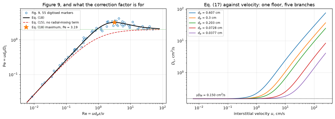
30 of the 55 digitised points lie above \(\mathrm{Pe} = 2\), the largest at 4.16. Eq. (15), molecular diffusion plus an uncorrected eddy term, has a supremum of exactly 2 and can therefore not produce any of them. That is not a matter of fitted constants: the eddy coefficient is \(\tfrac12\) because the mixing-cell limit is \(\mathrm{Pe} = 2\), so no choice of \(\gamma\) moves the ceiling. The maximum is the evidence for a third mechanism, and it is why the paper has an Eq. (16).
The experiment, simulated
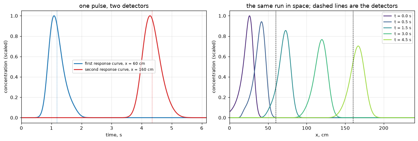
The forward problem at the conditions of their Figure 13: two response curves at the printed separation, the moments of each, and Eqs. (6) and (7) applied to the differences. Note how much of the second curve’s width is inherited from the first: that is exactly what the subtraction removes.
N13 = 1600
RUN1600 = simulate_experiment(U13, D13, dx_probe=DX13, n=N13, theta=0.5)
bed, t, c1, c2, dx13 = RUN1600
u_hat, D_hat, A1, A2 = invert_two_point(t, c1, c2, dx13)
A1m, t1m, s1m = moments(t, c1)
A2m, t2m, s2m = moments(t, c2)

fig, axes = plt.subplots(1, 2, figsize=(12.2, 4.2))
ax = axes[0]
ax.plot(t, c1 / c1.max(), color="tab:blue", lw=1.8,
        label=f"first response curve, x = {X1:.0f} cm")
ax.plot(t, c2 / c2.max(), color="tab:red", lw=1.8,
        label=f"second response curve, x = {X1 + DX13:.0f} cm")
for tt, col in ((t1m, "tab:blue"), (t2m, "tab:red")):
    ax.axvline(tt, color=col, lw=0.9, ls=":")
ax.set(xlabel="time, s", ylabel="concentration (scaled)",
       title="one pulse, two detectors", xlim=(0, t2m + 6 * np.sqrt(s2m)))
ax.legend(fontsize=8)

ax = axes[1]
b2 = TracerBed(bed.L, N13, U13, D13)
cs = emg(b2.x_c, X0, SIGMA, TAIL)
scale = cs.max()
dt2 = 0.5 * b2.h / U13
tt = 0.0
snaps = [0.0, 0.5, 1.5, 3.0, 4.5]
for target, col in zip(snaps, plt.cm.viridis(np.linspace(0.1, 0.85, len(snaps)))):
    while tt < target - 1e-12:
        cs = b2.step(cs, dt2, theta=0.5)
        tt += dt2
    ax.plot(b2.x_c, cs / scale, color=col, lw=1.5, label=f"t = {target:.1f} s")
for xx in (X1, X1 + DX13):
    ax.axvline(xx, color="k", lw=0.8, ls="--")
ax.set(xlabel="x, cm", ylabel="concentration (scaled)", xlim=(0, bed.L),
       title="the same run in space; dashed lines are the detectors")
ax.legend(fontsize=8)
fig.tight_layout()
plt.show()

display(Markdown(rf"""
| quantity | first curve | second curve | difference | E&R |
|---|---|---|---|---|
| area $A$ | {A1m:.6g} | {A2m:.6g} | ratio {A2m / A1m:.8f} | Eq. (5), $A_1=A_2$ |
| mean, s | {t1m:.4f} | {t2m:.4f} | {t2m - t1m:.4f} | Eq. (6), $\Delta x/u$ = {dx13 / U13:.4f} |
| variance, s² | {s1m:.5f} | {s2m:.5f} | {s2m - s1m:.5f} | Eq. (7), $2D_L\Delta x/u^3$ = {2 * D13 * dx13 / U13 ** 3:.5f} |

Inverting the two differences with Eqs. (6) and (7) on {N13} cells returns
$u$ = {u_hat:.5f} cm/s against the {U13:.5f} cm/s put in
({abs(dev(u_hat, U13)):.1e} relative) and $D_L$ = {D_hat:.5f} cm²/s against
{D13:.5f} ({abs(dev(D_hat, D13)):.1e}). The second curve's variance is
{s2m / s1m:.1f} times the first's, but only {(s2m - s1m) / s2m:.0%} of it is
what the bed between the detectors did; the rest is the injected pulse, and it
cancels.
"""))
| quantity | first curve | second curve | difference | E&R |
|---|---|---|---|---|
| area \(A\) | 0.030786 | 0.030786 | ratio 1.00000053 | Eq. (5), \(A_1=A_2\) |
| mean, s | 1.1819 | 4.3479 | 3.1660 | Eq. (6), \(\Delta x/u\) = 3.1660 |
| variance, s² | 0.06469 | 0.09048 | 0.02580 | Eq. (7), \(2D_L\Delta x/u^3\) = 0.02579 |
Inverting the two differences with Eqs. (6) and (7) on 1600 cells returns \(u\) = 31.60106 cm/s against the 31.60104 cm/s put in (4.9e-07 relative) and \(D_L\) = 4.06839 cm²/s against 4.06794 (1.1e-04). The second curve’s variance is 1.4 times the first’s, but only 29% of it is what the bed between the detectors did; the rest is the injected pulse, and it cancels.
What the grid measures instead of the bed
That recovery is not free. A first-order upwind convective flux adds a numerical diffusivity \(u h/2\), and a \(\theta\)-method in time adds \((\theta-\tfrac12)u^2 \Delta t\), for implicit Euler \(u^2\Delta t/2\). Neither is distinguishable from physical dispersion by any measurement, because they enter the equation in exactly the same place. So a tracer experiment simulated on a coarse grid reports its own truncation error as a dispersion coefficient.
A2.1 measures the steady-state version of this (\(u\,\mathrm dz/2\) masquerading as a lower Péclet number). Here it is in the transient inverse problem, and it is quantitative: the prediction is made before the runs, with no fitted constant.
LADDER = (400, 800, 1600, 3200)
SCHEMES = (("upwind, implicit Euler", None, 1.0),
           ("van Leer, implicit Euler", vanleer, 1.0),
           ("van Leer, Crank-Nicolson", vanleer, 0.5))
CFL = 0.5


def predicted_excess(h, limiter, theta, u=U13, cfl=CFL):
    """u h/2 for upwind plus (theta - 1/2) u^2 dt, dt = cfl h/u."""
    return (0.0 if limiter is not None else u * h / 2.0) + (theta - 0.5) * u ** 2 * cfl * h / u


rows = []
for n in LADDER:
    for tag, lim, th in SCHEMES:
        run = (RUN800 if (n, lim, th) == (N_ROUTE, vanleer, 0.5) else
               RUN1600 if (n, lim, th) == (N13, vanleer, 0.5) else
               simulate_experiment(U13, D13, dx_probe=DX13, n=n, cfl=CFL, theta=th,
                                   limiter=lim))
        uh, Dh, _, _ = invert_two_point(*run[1:])
        rows.append(dict(scheme=tag, n=n, h=run[0].h, D_hat=Dh, excess=Dh - D13, u_err=uh / U13 - 1,
                         predicted=predicted_excess(run[0].h, lim, th)))
tab = pd.DataFrame(rows)
tab["ratio"] = np.where(tab.predicted > 0, tab.excess / tab.predicted, np.nan)
tab["rel_err"] = np.abs(tab.D_hat / D13 - 1.0)

for tag, g in tab.groupby("scheme", sort=False):
    print(tag)
    for _, r in g.iterrows():
        extra = (f"predicted {r.predicted:8.5f}  ratio {r.ratio:6.4f}"
                 if r.predicted > 0 else "predicted 0 (both terms switched off)")
        print(f"   n = {int(r.n):5d}  h = {r.h:7.4f}  D_hat = {r.D_hat:9.5f}"
              f"  excess {r.excess:+9.5f}  {extra}")
    print()


def local_orders(err, h):
    err, h = np.asarray(err, float), np.asarray(h, float)
    return np.log(err[:-1] / err[1:]) / np.log(h[:-1] / h[1:])


cn = tab[tab.scheme == "van Leer, Crank-Nicolson"]
ie = tab[tab.scheme == "van Leer, implicit Euler"]
ORD_CN = local_orders(cn.rel_err, cn.h)
ORD_IE = local_orders(ie.rel_err, ie.h)
with_pred = tab.dropna(subset=["ratio"])
worst_ratio = float(np.abs(with_pred.ratio - 1).max())
coarse = tab.query("scheme == 'upwind, implicit Euler' and n == 400").D_hat.iloc[0]
ERR_CN_FINEST = float(cn[cn.n == LADDER[-1]].rel_err.iloc[0])
print("van Leer, Crank-Nicolson, observed order between successive grids: "
      + ", ".join(f"{o:.2f}" for o in ORD_CN))
display(Markdown(rf"""
The predicted excess is $u h/2$ for upwind plus $u^2\Delta t/2$ for implicit
Euler, with no fitted constant anywhere, and it accounts for the measured excess
to within **{worst_ratio:.1%}** over {len(with_pred)} runs and a factor of
{LADDER[-1] // LADDER[0]} in grid spacing. Switch both off (van Leer plus
Crank-Nicolson) and the recovered $D_L$ converges on the input at an observed
order between **{ORD_CN.min():.2f} and {ORD_CN.max():.2f}** on successive grids,
reaching {ERR_CN_FINEST:.1e} relative at $n$ = {LADDER[-1]}.

Read the first row the other way round and it is a warning about the
*experiment*, not about the code. A dispersion coefficient inferred from a pulse
is only as good as the resolution of whatever propagates it: at $n$ = {LADDER[0]}
the answer is {coarse / D13:.1f} times the truth, and the response curves it came
from look perfectly smooth.
"""))
upwind, implicit Euler
n = 400 h = 0.6000 D_hat = 18.28841 excess +14.22047 predicted 14.22047 ratio 1.0000
n = 800 h = 0.3000 D_hat = 11.17818 excess +7.11023 predicted 7.11023 ratio 1.0000
n = 1600 h = 0.1500 D_hat = 7.62306 excess +3.55512 predicted 3.55512 ratio 1.0000
n = 3200 h = 0.0750 D_hat = 5.84550 excess +1.77756 predicted 1.77756 ratio 1.0000
van Leer, implicit Euler
n = 400 h = 0.6000 D_hat = 8.82805 excess +4.76011 predicted 4.74016 ratio 1.0042
n = 800 h = 0.3000 D_hat = 6.44093 excess +2.37298 predicted 2.37008 ratio 1.0012
n = 1600 h = 0.1500 D_hat = 5.25338 excess +1.18544 predicted 1.18504 ratio 1.0003
n = 3200 h = 0.0750 D_hat = 4.66052 excess +0.59257 predicted 0.59252 ratio 1.0001
van Leer, Crank-Nicolson
n = 400 h = 0.6000 D_hat = 4.09747 excess +0.02952 predicted 0 (both terms switched off)
n = 800 h = 0.3000 D_hat = 4.07151 excess +0.00357 predicted 0 (both terms switched off)
n = 1600 h = 0.1500 D_hat = 4.06839 excess +0.00045 predicted 0 (both terms switched off)
n = 3200 h = 0.0750 D_hat = 4.06800 excess +0.00006 predicted 0 (both terms switched off)
van Leer, Crank-Nicolson, observed order between successive grids: 3.05, 3.00, 2.99The predicted excess is \(u h/2\) for upwind plus \(u^2\Delta t/2\) for implicit Euler, with no fitted constant anywhere, and it accounts for the measured excess to within 0.4% over 8 runs and a factor of 8 in grid spacing. Switch both off (van Leer plus Crank-Nicolson) and the recovered \(D_L\) converges on the input at an observed order between 2.99 and 3.05 on successive grids, reaching 1.4e-05 relative at \(n\) = 3200.
Read the first row the other way round and it is a warning about the experiment, not about the code. A dispersion coefficient inferred from a pulse is only as good as the resolution of whatever propagates it: at \(n\) = 400 the answer is 4.5 times the truth, and the response curves it came from look perfectly smooth.
Where the correlation says dispersion matters
Eq. (17) is usually wanted for one purpose: deciding whether a bed can be treated as plug flow. The bed Péclet number is \(\mathrm{Pe}_L = uL/D_L =
(L/d_p)\,\mathrm{Pe}\), so the correlation and the aspect ratio settle it between them. What a given \(\mathrm{Pe}_L\) then does to conversion is A2.1’s subject and is not rebuilt here.
L_over_dp = np.logspace(0.7, 3.2, 220)
Re_ax = np.logspace(np.log10(P["reynolds_min"]), np.log10(P["reynolds_max"]), 220)
G_R, G_L = np.meshgrid(Re_ax, L_over_dp)
PeL = G_L * Pe_eq18(G_R)

fig, ax = plt.subplots(figsize=(7.0, 4.4))
cf = ax.contourf(G_R, G_L, np.log10(PeL), levels=np.linspace(-1, 4.5, 23),
                 cmap="viridis")
cl = ax.contour(G_R, G_L, PeL, levels=[1, 10, 100, 1000], colors="w", linewidths=1.1)
ax.clabel(cl, fmt="Pe_L = %g", fontsize=8)
ax.set(xscale="log", yscale="log", xlabel=r"$\mathrm{Re}$", ylabel=r"$L/d_p$",
       title="bed Peclet number from Eq. (18), argon in air")
fig.colorbar(cf, ax=ax, label=r"$\log_{10}\mathrm{Pe}_L$")
ax.grid(alpha=0.25, color="w")
fig.tight_layout()
plt.show()

RE_SLOW, RE_FAST, L_DP, PE_L_NEED = 0.01, 10.0, 100.0, 100.0


def plug_flow_numbers(A=A_printed, B=B_printed):
    """Pe_L of a bed L_DP particles deep at RE_SLOW and RE_FAST, and the depth
    that reaches PE_L_NEED at RE_SLOW and at the Peclet maximum."""
    Pe_s, Pe_f = Pe_eq18(RE_SLOW, A, B), Pe_eq18(RE_FAST, A, B)
    return L_DP * Pe_s, L_DP * Pe_f, PE_L_NEED / Pe_s, PE_L_NEED / Pe_max_eq18(A, B)[1]


PEL_SLOW, PEL_FAST, LDP_SLOW, LDP_MAX = plug_flow_numbers()
display(Markdown(rf"""
The map is read along a horizontal line. A bed {L_DP:.0f} particles deep runs at
$\mathrm{{Pe}}_L$ = {PEL_SLOW:.1f} at $\mathrm{{Re}}$ = {RE_SLOW} but
{PEL_FAST:.0f} at $\mathrm{{Re}}$ = {RE_FAST:.0f}: the *same bed*, two orders of
magnitude apart in how nearly it is plug flow, because at low Reynolds number
$D_L$ stops falling with velocity and sits on the molecular floor
$\gamma D_M$ = {gamma * D_M:.3f} cm²/s. Reaching $\mathrm{{Pe}}_L$ =
{PE_L_NEED:.0f} needs $L/d_p$ = {LDP_SLOW:.0f} at $\mathrm{{Re}}$ = {RE_SLOW}
and only {LDP_MAX:.0f} at the Péclet maximum, $\mathrm{{Re}}$ = {Re_star:.1f}.

That is the practical content of the molecular-diffusion term, and it is why a
correlation carrying only the eddy branch would mislead badly in exactly the
regime (slow flow, small particles) where laboratory reactors live.
"""))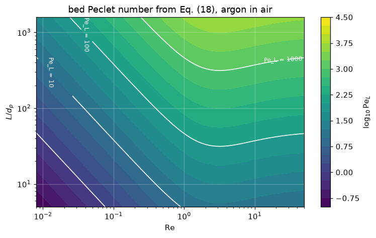
The map is read along a horizontal line. A bed 100 particles deep runs at \(\mathrm{Pe}_L\) = 2.6 at \(\mathrm{Re}\) = 0.01 but 269 at \(\mathrm{Re}\) = 10: the same bed, two orders of magnitude apart in how nearly it is plug flow, because at low Reynolds number \(D_L\) stops falling with velocity and sits on the molecular floor \(\gamma D_M\) = 0.150 cm²/s. Reaching \(\mathrm{Pe}_L\) = 100 needs \(L/d_p\) = 3800 at \(\mathrm{Re}\) = 0.01 and only 31 at the Péclet maximum, \(\mathrm{Re}\) = 3.2.
That is the practical content of the molecular-diffusion term, and it is why a correlation carrying only the eddy branch would mislead badly in exactly the regime (slow flow, small particles) where laboratory reactors live.
The fine-particle anomaly, and what their own diagnostic says about it
With the finest beads, the sand and the diakon, Edwards and Richardson’s moment analysis returned dispersion coefficients far above Eq. (17); Figure 15 prints one such apparent \(D_L\). They then applied their own consistency test, computing the second response curve from the first with that \(D_L\), and found the measured curve peaked earlier than the computed one. They attributed it to channelling: the materials “have a fair spread of particle sizes … it is thought that channels are being formed, the fine particles being swept aside laterally”.
The moment method cannot itself tell a genuinely larger \(D_L\) from a velocity distribution, because it only ever sees two moments. The shape can. So the question a solver can answer is: what velocity structure reproduces both their \(D_L\) and the sign of their shape discrepancy? The model is TwoZoneBed, with \(\kappa\) set in every case so that the two-point moment method returns their apparent \(D_L\).
UMF15 = voidage_of(DP15, "u_mf_cm_s")
U_OVER_UMF15 = U15 * EPS15 / UMF15
print(f"Figure 15 conditions: d_p = {DP15} cm, Re = {RE15}, "
      f"apparent D_L = {DL15} cm2/s")
print(f"  voidage (Table 1)                       {EPS15}")
print(f"  interstitial velocity                   {U15:.4f} cm/s")
print(f"  superficial velocity                    {U15 * EPS15:.4f} cm/s")
print(f"  minimum fluidisation velocity (Table 1) {UMF15} cm/s"
      f"   -> the run sits at {U_OVER_UMF15:.0%} of it")
print(f"  Eq. (17) prediction                     {D15:.5f} cm2/s")
print(f"  measured / predicted                    {DL15 / D15:.2f}"
      f"   (deviation {dev(D15, DL15):+.1%})")
Figure 15 conditions: d_p = 0.0097 cm, Re = 0.071, apparent D_L = 0.503 cm2/s
voidage (Table 1) 0.41
interstitial velocity 2.6351 cm/s
superficial velocity 1.0804 cm/s
minimum fluidisation velocity (Table 1) 1.23 cm/s -> the run sits at 88% of it
Eq. (17) prediction 0.14981 cm2/s
measured / predicted 3.36 (deviation -70.2%)# DX_ASSUMED. Figure 15's legend prints the bead size, the Reynolds number and
# the apparent D_L, and NOT the detector separation. E&R p. 111 say the test
# section was "either of two tubes", and their conclusions quote the range of
# separations. Everything below ASSUMES the section Figure 13 prints; the
# alternative is run at the end of this section, and it is not a small difference.
DX_ASSUMED = DX13
FLUX_FRACS = (0.01, 0.03, 0.05, 0.08, 0.25, 0.40, 0.60, 0.80)
N_FLUX = 800
def fine_case(flux_frac, **kw):
"""channelling_case at the Figure-15 conditions, tuned to E&R's apparent D_L."""
kw.setdefault("dx_probe", DX_ASSUMED)
return channelling_case(flux_frac, U15, D15, DL15, **kw)
def flux_scan(**kw):
out = {ff: fine_case(ff, n=N_FLUX, **kw) for ff in FLUX_FRACS}
df = pd.DataFrame([{k: v for k, v in r.items() if k not in ("t", "sim", "comp", "first")}
for r in out.values()])
df["u1_over_u"], df["u2_over_u"] = df.u1 / U15, df.u2 / U15
df["slow_minority"] = df.u1 < df.u2 # zone 1 holds the minority volume
return df, out
scan, SCAN_RUNS = flux_scan()
print(f"The minority zone holds {scan.th1.iloc[0]:.0%} of the void. kappa is set in every row")
print(f"so that the two-point moment method returns E&R's measured {DL15} cm2/s.\n")
print(scan[["flux_frac", "u1_over_u", "u2_over_u", "kappa", "D_hat", "lag", "resid"]]
.to_string(index=False,
formatters={"flux_frac": "{:.2f}".format,
"u1_over_u": "{:.3f}".format,
"u2_over_u": "{:.3f}".format,
"kappa": "{:.3f}".format,
"D_hat": "{:.4f}".format,
"lag": "{:+.2%}".format,
"resid": "{:.1%}".format}))The minority zone holds 15% of the void. kappa is set in every row
so that the two-point moment method returns E&R's measured 0.503 cm2/s.
flux_frac u1_over_u u2_over_u kappa D_hat lag resid
0.01 0.067 1.165 0.385 0.5033 +0.23% 3.3%
0.03 0.200 1.141 0.283 0.5033 +0.27% 3.8%
0.05 0.333 1.118 0.197 0.5033 +0.32% 4.5%
0.08 0.533 1.082 0.096 0.5033 +0.36% 6.3%
0.25 1.667 0.882 0.197 0.5032 -0.23% 3.6%
0.40 2.667 0.706 1.229 0.5032 -0.11% 1.2%
0.60 4.000 0.471 3.981 0.5032 -0.04% 0.6%
0.80 5.333 0.235 8.306 0.5032 -0.03% 0.3%# The scan above holds the minority VOLUME fixed and moves the flow split. That
# is one slice of the parameter space, and the peak displacement it bounds is a
# maximum over that slice only. Here the volume fraction moves too, with the
# velocity RATIO held fixed, so that every row is still tuned to the same
# measured D_L. Both directions are run: the minority zone slow, and fast.
#
# A bed with (th1, u1/u2) is the bed (1 - th1, u2/u1) with the zones renamed, so
# only th1 < 0.5 is scanned: the other half would repeat each bed. The cell
# checks that once.
SLOW, FAST = 0.2, 5.0 # u1/u2 for the two directions
TH_SCAN = (0.03, 0.05, 0.15, 0.35)
N_SPLIT, N_COARSE, N_FINE = 1000, 500, 2000 # production grid, and the ladder
LAG_FLOOR = 0.0005 # 0.05 % of the transit time
def split_case(th1, ratio, n=N_SPLIT, **kw):
return two_zone_split(th1, ratio, U15, D15, DL15, n=n, dx_probe=DX_ASSUMED, **kw)
def split_scan(n=N_SPLIT, **kw):
rows = []
for th1 in TH_SCAN:
for ratio in (SLOW, FAST):
r = split_case(th1, ratio, n=n, **kw)
# zone 1 is the minority by volume here, so it is slow when ratio < 1
rows.append(dict(th1=th1, ratio=ratio, minority_slow=ratio < 1.0,
D_hat=r["D_hat"], lag=r["lag"], resid=r["resid"]))
df = pd.DataFrame(rows)
df["expected_sign"] = np.where(df.minority_slow, 1.0, -1.0)
df["sign_ok"] = np.sign(df.lag) == df.expected_sign
return df
th_scan = split_scan()
th_coarse = split_scan(n=N_COARSE) # the coarse rung of the ladder
_ref, _mirror = split_case(0.15, SLOW), split_case(0.85, FAST)
MIRROR_GAP = abs(_mirror["lag"] - _ref["lag"]) + abs(_mirror["resid"] - _ref["resid"])
print("Volume split scanned at fixed velocity ratio; kappa retuned every row.")
print("'minority_slow' is whether the zone holding LESS of the void is the slower one;")
print(f"'sign_ok' is whether the computed peak then lags, as E&R report. n = {N_SPLIT}.\n")
print(th_scan.drop(columns="expected_sign").assign(lag_n500=th_coarse.lag).to_string(
index=False, formatters={"th1": "{:.2f}".format, "ratio": "{:.1f}".format,
"D_hat": "{:.4f}".format, "lag": "{:+.3%}".format,
"lag_n500": "{:+.3%}".format, "resid": "{:.1%}".format}))
print(f"\nthe same bed with the zones renamed, th1 = 0.85 at u1/u2 = {FAST:g} against"
f" th1 = 0.15 at {SLOW:g}: lag and residual differ by (here {MIRROR_GAP:.1e})")
sign_ok = int(th_scan.sign_ok.sum())
sign_ok_coarse = int(th_coarse.sign_ok.sum())
flux_ok = int((np.sign(scan.lag) == np.where(scan.slow_minority, 1, -1)).sum())
above = th_scan[th_scan.lag.abs() > LAG_FLOOR]
bad_coarse = th_coarse[~th_coarse.sign_ok]
print(f"\nsign follows minority-by-volume-slow in {sign_ok} of {len(th_scan)}"
f" beds here and {flux_ok} of {len(scan)} in the flux scan above;")
print(f"{len(above)} of the {len(th_scan)} beds displace the peak by more than {LAG_FLOOR:.2%}.")
print(f"on {N_COARSE} cells the sign rule holds in {sign_ok_coarse} of {len(th_coarse)}; the"
" exception(s) at th1 = " + (", ".join(f"{v:.2f}" for v in bad_coarse.th1) or "none")
+ " are the coarse grid's.")
LAG_MAX_CLASS = float(th_scan.lag.abs().max())
LAG_MAX_SLICE = float(scan.lag.abs().max())
print(f"largest peak lag anywhere: {LAG_MAX_CLASS:.2%} of the transit"
f" time, at th1 = {th_scan.loc[th_scan.lag.abs().idxmax(), 'th1']:.2f};"
f" largest shape residual: {th_scan.resid.max():.1%} of peak")
print(f"the th1 = {TH1} slice reported above tops out at"
f" {LAG_MAX_SLICE:.2%} and {scan.resid.max():.1%}, so a maximum over one slice")
print("is not a maximum over the model class (the ratio on matched grids follows).")
# The ladder: every bed of the split scan one grid finer, and the flow-scan maximum
# with the split-scan maximum on matched grids.
th_fine = split_scan(n=N_FINE)
LAG_CHANGE = (th_fine.lag / th_scan.lag - 1).abs()
LAG_CHANGE_COARSE = (th_scan.lag / th_coarse.lag - 1).abs()
SIGN_OK_FINE = int(th_fine.sign_ok.sum())
ABOVE_FINE = th_fine[th_fine.lag.abs() > LAG_FLOOR]
I_MAX = int(th_scan.lag.abs().idxmax()) # the bed of the largest lag
RESID_CHANGE = abs(th_fine.resid.iloc[I_MAX] / th_scan.resid.iloc[I_MAX] - 1)
RESID_CHANGE_COARSE = abs(th_scan.resid.iloc[I_MAX] / th_coarse.resid.iloc[I_MAX] - 1)
print(f"\nthe split scan on {N_COARSE}, {N_SPLIT} and {N_FINE} cells:")
print(th_scan[["th1", "ratio", "minority_slow"]].assign(
lag_n500=th_coarse.lag, lag_n1000=th_scan.lag, lag_n2000=th_fine.lag,
change=LAG_CHANGE).to_string(index=False, formatters={
"th1": "{:.2f}".format, "ratio": "{:.1f}".format, "lag_n500": "{:+.3%}".format,
"lag_n1000": "{:+.3%}".format, "lag_n2000": "{:+.3%}".format,
"change": "{:.1%}".format}))
CHANGE_SLOW = float(LAG_CHANGE[th_scan.minority_slow].max())
CHANGE_FAST = float(LAG_CHANGE[~th_scan.minority_slow].max())
print(f"largest change of a lag from {N_SPLIT} to {N_FINE} cells: {CHANGE_FAST:.0%} where the"
f" minority zone is fast, {CHANGE_SLOW:.1%} where it is slow;")
print(f"on {N_FINE} cells the sign rule holds in {SIGN_OK_FINE} of {len(th_fine)} beds,"
f" {len(ABOVE_FINE)} of them above {LAG_FLOOR:.2%}; the largest residual moves by"
f" {RESID_CHANGE:.1%}.")
N_MATCH = (2 * N_FLUX, 4 * N_FLUX) # 1600 and 3200 cells, for both scans
FF_MAX = float(scan.loc[scan.lag.abs().idxmax(), "flux_frac"])
_th_max, _r_max = th_scan.th1.iloc[I_MAX], th_scan.ratio.iloc[I_MAX]
MATCH = {n: (abs(split_case(_th_max, _r_max, n=n)["lag"]), abs(fine_case(FF_MAX, n=n)["lag"]))
for n in N_MATCH}
print(f"\nmatched grids: largest split-scan lag (th1 = {_th_max:.2f}, u1/u2 = {_r_max:g}) and"
f" largest flow-scan lag (share {FF_MAX:.2f})")
print(f" n = {N_FLUX:5d} / {N_SPLIT}: {LAG_MAX_CLASS:.3%} and {LAG_MAX_SLICE:.3%} (the scans above)")
for n, (lc, ls) in MATCH.items():
print(f" n = {n:5d}: {lc:.3%} and {ls:.3%}, ratio {lc / ls:.2f}")
RATIO_MATCH = {n: lc / ls for n, (lc, ls) in MATCH.items()}
LAG_SLICE_FINE = MATCH[N_MATCH[-1]][1]
LAG_CLASS_FINE = MATCH[N_MATCH[-1]][0]Volume split scanned at fixed velocity ratio; kappa retuned every row.
'minority_slow' is whether the zone holding LESS of the void is the slower one;
'sign_ok' is whether the computed peak then lags, as E&R report. n = 1000.
th1 ratio minority_slow D_hat lag resid sign_ok lag_n500
0.03 0.2 True 0.5032 +1.330% 18.0% True +1.139%
0.03 5.0 False 0.5031 -0.330% 4.9% True -0.215%
0.05 0.2 True 0.5032 +1.063% 12.8% True +0.981%
0.05 5.0 False 0.5031 -0.195% 3.0% True -0.129%
0.15 0.2 True 0.5031 +0.279% 3.7% True +0.164%
0.15 5.0 False 0.5031 -0.113% 1.0% True -0.114%
0.35 0.2 True 0.5031 +0.055% 0.9% True -0.011%
0.35 5.0 False 0.5031 -0.024% 0.2% True -0.004%
the same bed with the zones renamed, th1 = 0.85 at u1/u2 = 5 against th1 = 0.15 at 0.2: lag and residual differ by (here 7.0e-15)
sign follows minority-by-volume-slow in 8 of 8 beds here and 8 of 8 in the flux scan above;
7 of the 8 beds displace the peak by more than 0.05%.
on 500 cells the sign rule holds in 7 of 8; the exception(s) at th1 = 0.35 are the coarse grid's.
largest peak lag anywhere: 1.33% of the transit time, at th1 = 0.03; largest shape residual: 18.0% of peak
the th1 = 0.15 slice reported above tops out at 0.36% and 6.3%, so a maximum over one slice
is not a maximum over the model class (the ratio on matched grids follows).
the split scan on 500, 1000 and 2000 cells:
th1 ratio minority_slow lag_n500 lag_n1000 lag_n2000 change
0.03 0.2 True +1.139% +1.330% +1.350% 1.5%
0.03 5.0 False -0.215% -0.330% -0.385% 16.9%
0.05 0.2 True +0.981% +1.063% +1.084% 1.9%
0.05 5.0 False -0.129% -0.195% -0.246% 26.1%
0.15 0.2 True +0.164% +0.279% +0.293% 4.9%
0.15 5.0 False -0.114% -0.113% -0.112% 0.9%
0.35 0.2 True -0.011% +0.055% +0.059% 7.9%
0.35 5.0 False -0.004% -0.024% -0.035% 47.8%
largest change of a lag from 1000 to 2000 cells: 48% where the minority zone is fast, 7.9% where it is slow;
on 2000 cells the sign rule holds in 8 of 8 beds, 7 of them above 0.05%; the largest residual moves by 1.2%.
matched grids: largest split-scan lag (th1 = 0.03, u1/u2 = 0.2) and largest flow-scan lag (share 0.08)
n = 800 / 1000: 1.330% and 0.360% (the scans above)
n = 1600: 1.348% and 0.460%, ratio 2.93
n = 3200: 1.345% and 0.493%, ratio 2.73FF_SLOW, FF_FAST = 0.03, 0.40
slow, fast = SCAN_RUNS[FF_SLOW], SCAN_RUNS[FF_FAST]
fig, axes = plt.subplots(1, 2, figsize=(12.2, 4.4), sharey=True)
for ax, case, ttl in ((axes[0], slow, "minority zone SLOW (a stagnant pocket)"),
(axes[1], fast, "minority zone FAST (a channel)")):
t_, sim, comp = case["t"], case["sim"], case["comp"]
pk = sim.max()
ax.plot(t_, sim / pk, color="k", lw=2.0,
label="two-zone bed (the 'measurement')")
ax.plot(t_, comp / comp.max(), "o", ms=3.2, mfc="none", color="tab:red",
markevery=max(1, len(t_) // 60),
label=r"computed from the first curve with the fitted $D_L$")
ax.axvline(peak_time(t_, sim), color="k", lw=0.8, ls=":")
ax.axvline(peak_time(t_, comp), color="tab:red", lw=0.8, ls=":")
lo = peak_time(t_, sim)
ax2 = ax.twinx()
ax2.plot(t_, 100 * (comp / comp.max() - sim / pk), color="tab:blue", lw=1.3)
ax2.axhline(0.0, color="tab:blue", lw=0.6, ls=":")
ax2.set_ylim(-4.0, 4.0)
ax2.set_ylabel("computed - simulated, % of peak", color="tab:blue",
fontsize=8)
ax2.tick_params(axis="y", labelcolor="tab:blue", labelsize=8)
ax2.grid(False)
ax.set(xlabel="time, s", xlim=(lo - 8, lo + 16),
title=f"{ttl}\ncomputed peak {case['lag']:+.2%} of transit time")
ax.legend(fontsize=8, loc="upper left")
axes[0].set_ylabel("concentration (scaled)")
fig.tight_layout()
plt.show()
# is the sign an artefact of the injected pulse shape? repeat with a nearly symmetric one
TAIL_SYM = 0.4
sym_slow = fine_case(FF_SLOW, tail=TAIL_SYM, n=N_FLUX)
sym_fast = fine_case(FF_FAST, tail=TAIL_SYM, n=N_FLUX)
def sigma_over_tbar(dx, u=U15, D=DL15):
"""sqrt(2 D dx/u^3) / (dx/u) at E&R's apparent D_L: falls as dx^-1/2."""
return np.sqrt(2 * D * dx / u ** 3) / (dx / u)
sig_t, sig_t_alt = sigma_over_tbar(DX_ASSUMED), sigma_over_tbar(DX_SHORT)
alt = fine_case(FF_SLOW, n=N_FLUX, dx_probe=DX_SHORT)
res_slow, res_fast = slow["resid"], fast["resid"]
fast_lags = scan.loc[~scan.slow_minority, "lag"]
display(Markdown(rf"""
**The sign of E&R's shape discrepancy picks out the slow zone, not the fast
one.** Constrained to reproduce their measured $D_L$ = {DL15} cm²/s, the
two-zone bed makes the computed curve peak *later* than the simulated one (the
sense they report) only when the zone holding the smaller share of the void is
the **slower** one. With a fast channel the sign is the wrong way round in every
case tried, between {fast_lags.min():+.2%} and {fast_lags.max():+.2%}. Nor is it
an artefact of the injected pulse: repeating the two runs with a nearly symmetric
injection instead of the long-tailed one gives {sym_slow['lag']:+.2%} and
{sym_fast['lag']:+.2%}, the same signs.
**How far that generalises, tested rather than assumed.** Scanning the volume
split as well ($\theta_1$ from {min(TH_SCAN):.2f} to {max(TH_SCAN):.2f} in zone 1,
each direction, every bed still tuned to the same measured $D_L$, and each bed
counted once, since $(\theta_1, u_1/u_2)$ and $(1-\theta_1, u_2/u_1)$ are the
same bed), the sign follows minority-by-volume-slow in **{sign_ok} of
{len(th_scan)}** beds on {N_SPLIT} cells, including the ones where the minority
zone is the fast one; {len(above)} of them displace the peak by more than
{LAG_FLOOR:.2%} of the transit time. On {N_COARSE} cells the rule fails in
{len(th_coarse) - sign_ok_coarse} bed(s), at $\theta_1$ =
{", ".join(f"{v:.2f}" for v in bad_coarse.th1) or "none"}, where the lag is
small; refined, the sign is the rule's. On {N_FINE} cells it holds in
{SIGN_OK_FINE} of {len(th_fine)}, {len(ABOVE_FINE)} of them above the floor. The
lags themselves are values at their grid. Every bed was run one grid finer: where
the minority zone is slow the lag changes by at most {CHANGE_SLOW:.1%}, where it is
fast by up to {CHANGE_FAST:.0%}, so the fast-minority lags are grid values good
to about {CHANGE_FAST:.0%}, not converged numbers. No sign changes. So the claim the page makes is the conditional one: *when* a
two-zone bed at this $D_L$ displaces the peak measurably, the direction E&R
report is the one a slow minority zone gives.
**What is small is the peak displacement, not the asymmetry, and how small
depends on where you look.** At the published slice, $\theta_1$ = {TH1}, the
largest lag is {LAG_MAX_SLICE:.2%} of the transit time on {N_FLUX} cells and
{LAG_SLICE_FINE:.2%} on {N_MATCH[-1]}, far below what a chart recorder
resolves. That is a maximum over one slice, not over the model class: letting
the volume fraction move as well, still tuned to the same measured $D_L$, reaches
**{LAG_MAX_CLASS:.2%}** at $\theta_1$ = {_th_max:.2f} ({LAG_CLASS_FINE:.2%} on
{N_MATCH[-1]} cells). On matched grids the ratio of the two maxima is
{RATIO_MATCH[N_MATCH[0]]:.2f} on {N_MATCH[0]} cells and
{RATIO_MATCH[N_MATCH[-1]]:.2f} on {N_MATCH[-1]}, and the shape residual reaches
{th_scan.resid.max():.1%} of peak (it moves by {RESID_CHANGE:.1%} on {N_FINE} cells). So the peak displacement bounds
nothing about the model class; what it says is that in the regime E&R's own
picture describes, the discrepancy is mostly *shape*. The blue traces above are
the computed curve minus the simulated one, spanning {res_slow:.1%} of the peak
in the slow case against {res_fast:.1%} in the fast one.
**Is that visible to them?** Not answerable from the paper, and the page does
not claim it is. Appendix A gives percentage standard deviations of a five-pulse
average ({P['percent_sd_pulse_area']} % in area and
{P['percent_sd_pulse_variance']} % in variance), but those are the scatter of
*integrated moments*, and a residual of a few per cent of the peak is a
*pointwise* quantity. The two are not commensurable: a standard deviation
on an integral bounds pointwise noise neither above nor below. The only
pointwise statement in the paper is that below about $c_\mathrm{{max}}$/30 "the
noise level becomes too great for accurate measurements" (p. 114), which is a
statement about the tail, not the peak. So the residual is **comparable to, but
not demonstrably above, their reported reproducibility**, and what a two-zone
bed at their measured $D_L$ produces is a discrepancy of the size they would
have had to argue about, not one this page can show they must have seen.
**Δx is assumed, and it matters.** Figure 15's legend prints {DP15} cm beads,
$\mathrm{{Re}}$ = {RE15} and $D_L$ = {DL15} cm²/s, and **not** the detector
separation. Everything above takes $\Delta x$ = {DX_ASSUMED:.0f} cm, which is
what Figure 13 prints for the large-particle run; the paper's other test section
was {DX_SHORT} cm. At {DX_ASSUMED:.0f} cm the response curve has
$\sigma/\bar t$ = {sig_t:.1%}, close to plug flow, so there is not much shape for
a velocity distribution to distort. At {DX_SHORT} cm it is {sig_t_alt:.1%},
{sig_t_alt / sig_t:.1f} times larger, so that argument would be weaker at the
shorter section, but running it is not the same as arguing it. The same
slow-zone case at {DX_SHORT} cm gives a lag of {alt['lag']:+.2%} against
{slow['lag']:+.2%}, and a shape residual of {alt['resid']:.1%} of peak against
{res_slow:.1%}: the sign is unchanged and the discrepancy gets
**{"smaller" if alt['resid'] < res_slow else "larger"}**, because the shorter
section also gives the two zones less distance in which to differentiate. The
$\sigma/\bar t$ scaling alone predicts the wrong direction here, which is the
reason to run the alternative rather than reason about it. What survives either
way: the sign, and the fact that the shape residual is much larger than the peak
displacement.
A discrepancy large enough to see on a chart recorder therefore implies
**either** a slow region rather than a channel, **or** structure coarser than
any two-zone description tuned to {DL15} cm²/s can hold, for instance an
exchange so slow that the apparent $D_L$ is still growing with bed length, which
the two-point method would faithfully report as a length-dependent "dispersion
coefficient". The scan does not choose between those two branches, and the
metadata for this page must not either.
E&R checked for a length dependence and found none, but only for the *large*
particles, over {DX_SHORT} to {DX_LONG} cm. For the fine particles the check is
not reported, and it is exactly the measurement that would settle both this and
the $\Delta x$ assumption above.
**What this does not do.** It does not fit their response curves: those are not
tabulated and Figure 15's abscissa carries no scale. It reproduces the sign and
the order of magnitude of a diagnostic from their printed $D_L$ and their
printed conditions, and it says which of two channelling pictures is consistent
with it.
"""))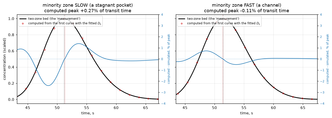
The sign of E&R’s shape discrepancy picks out the slow zone, not the fast one. Constrained to reproduce their measured \(D_L\) = 0.503 cm²/s, the two-zone bed makes the computed curve peak later than the simulated one (the sense they report) only when the zone holding the smaller share of the void is the slower one. With a fast channel the sign is the wrong way round in every case tried, between -0.23% and -0.03%. Nor is it an artefact of the injected pulse: repeating the two runs with a nearly symmetric injection instead of the long-tailed one gives +0.38% and -0.15%, the same signs.
How far that generalises, tested rather than assumed. Scanning the volume split as well (\(\theta_1\) from 0.03 to 0.35 in zone 1, each direction, every bed still tuned to the same measured \(D_L\), and each bed counted once, since \((\theta_1, u_1/u_2)\) and \((1-\theta_1, u_2/u_1)\) are the same bed), the sign follows minority-by-volume-slow in 8 of 8 beds on 1000 cells, including the ones where the minority zone is the fast one; 7 of them displace the peak by more than 0.05% of the transit time. On 500 cells the rule fails in 1 bed(s), at \(\theta_1\) = 0.35, where the lag is small; refined, the sign is the rule’s. On 2000 cells it holds in 8 of 8, 7 of them above the floor. The lags themselves are values at their grid. Every bed was run one grid finer: where the minority zone is slow the lag changes by at most 7.9%, where it is fast by up to 48%, so the fast-minority lags are grid values good to about 48%, not converged numbers. No sign changes. So the claim the page makes is the conditional one: when a two-zone bed at this \(D_L\) displaces the peak measurably, the direction E&R report is the one a slow minority zone gives.
What is small is the peak displacement, not the asymmetry, and how small depends on where you look. At the published slice, \(\theta_1\) = 0.15, the largest lag is 0.36% of the transit time on 800 cells and 0.49% on 3200, far below what a chart recorder resolves. That is a maximum over one slice, not over the model class: letting the volume fraction move as well, still tuned to the same measured \(D_L\), reaches 1.33% at \(\theta_1\) = 0.03 (1.34% on 3200 cells). On matched grids the ratio of the two maxima is 2.93 on 1600 cells and 2.73 on 3200, and the shape residual reaches 18.0% of peak (it moves by 1.2% on 2000 cells). So the peak displacement bounds nothing about the model class; what it says is that in the regime E&R’s own picture describes, the discrepancy is mostly shape. The blue traces above are the computed curve minus the simulated one, spanning 3.8% of the peak in the slow case against 1.2% in the fast one.
Is that visible to them? Not answerable from the paper, and the page does not claim it is. Appendix A gives percentage standard deviations of a five-pulse average (1.37 % in area and 1.3 % in variance), but those are the scatter of integrated moments, and a residual of a few per cent of the peak is a pointwise quantity. The two are not commensurable: a standard deviation on an integral bounds pointwise noise neither above nor below. The only pointwise statement in the paper is that below about \(c_\mathrm{max}\)/30 “the noise level becomes too great for accurate measurements” (p. 114), which is a statement about the tail, not the peak. So the residual is comparable to, but not demonstrably above, their reported reproducibility, and what a two-zone bed at their measured \(D_L\) produces is a discrepancy of the size they would have had to argue about, not one this page can show they must have seen.
Δx is assumed, and it matters. Figure 15’s legend prints 0.0097 cm beads, \(\mathrm{Re}\) = 0.071 and \(D_L\) = 0.503 cm²/s, and not the detector separation. Everything above takes \(\Delta x\) = 100 cm, which is what Figure 13 prints for the large-particle run; the paper’s other test section was 21.3 cm. At 100 cm the response curve has \(\sigma/\bar t\) = 6.2%, close to plug flow, so there is not much shape for a velocity distribution to distort. At 21.3 cm it is 13.4%, 2.2 times larger, so that argument would be weaker at the shorter section, but running it is not the same as arguing it. The same slow-zone case at 21.3 cm gives a lag of +0.23% against +0.27%, and a shape residual of 1.7% of peak against 3.8%: the sign is unchanged and the discrepancy gets smaller, because the shorter section also gives the two zones less distance in which to differentiate. The \(\sigma/\bar t\) scaling alone predicts the wrong direction here, which is the reason to run the alternative rather than reason about it. What survives either way: the sign, and the fact that the shape residual is much larger than the peak displacement.
A discrepancy large enough to see on a chart recorder therefore implies either a slow region rather than a channel, or structure coarser than any two-zone description tuned to 0.503 cm²/s can hold, for instance an exchange so slow that the apparent \(D_L\) is still growing with bed length, which the two-point method would faithfully report as a length-dependent “dispersion coefficient”. The scan does not choose between those two branches, and the metadata for this page must not either.
E&R checked for a length dependence and found none, but only for the large particles, over 21.3 to 121.3 cm. For the fine particles the check is not reported, and it is exactly the measurement that would settle both this and the \(\Delta x\) assumption above.
What this does not do. It does not fit their response curves: those are not tabulated and Figure 15’s abscissa carries no scale. It reproduces the sign and the order of magnitude of a diagnostic from their printed \(D_L\) and their printed conditions, and it says which of two channelling pictures is consistent with it.
umf_sand = float(tab1.loc[tab1.material == "sand", "u_mf_cm_s"].iloc[0])
umf_diakon = float(tab1.loc[tab1.material == "diakon", "u_mf_cm_s"].iloc[0])
display(Markdown(rf"""
### One number that bears on their explanation, from Table 1 alone, and the sentence that cuts against it

At $\mathrm{{Re}}$ = {RE15} the superficial velocity is {U15 * EPS15:.3f} cm/s,
and Table 1 gives the minimum fluidisation velocity of those same {DP15} cm
beads as {UMF15} cm/s. The anomalous run therefore sits at
**{U_OVER_UMF15:.0%} of incipient fluidisation**, a number the paper never
states, from two printed values on different pages, transcribed independently.

It is offered as corroboration because of what E&R write on p. 120: "the
transition is sharper with the material with the narrowest size range, occurring
only at velocities near those giving rise to bed expansion". But **the sentence
immediately before that one, in the same paragraph, points the other way**:
"However, this phenomenon occurs at velocities considerably below those at which
either bed expansion or fluidisation takes place."

Both sentences are printed, three lines apart, and the paper is in tension with
itself here. {U_OVER_UMF15:.0%} of $u_\mathrm{{mf}}$ is what the *quoted*
sentence would lead you to expect and is hard to call "considerably below", so
the number corroborates one half of the paragraph and sits awkwardly against the
other. Quoting only the half it agrees with would be the easy version of this
paragraph and the wrong one.

Two further limits on what {U_OVER_UMF15:.0%} can carry. Table 1 prints that
$u_\mathrm{{mf}}$ as the authors' own value for that size, and the anomaly is
reported for the sand and the diakon as well, whose tabulated $u_\mathrm{{mf}}$
are {umf_sand} and {umf_diakon} cm/s against Figure 15's single quoted run. So
what the number establishes is narrower than "the bed was near fluidisation": it
is that this particular run was not in a regime where incipient fluidisation is
orders of magnitude away, so a mechanism involving particle motion is not
excluded on velocity grounds, while the sentence above says the authors saw the
effect where it was.
"""))
One number that bears on their explanation, from Table 1 alone, and the sentence that cuts against it
At \(\mathrm{Re}\) = 0.071 the superficial velocity is 1.080 cm/s, and Table 1 gives the minimum fluidisation velocity of those same 0.0097 cm beads as 1.23 cm/s. The anomalous run therefore sits at 88% of incipient fluidisation, a number the paper never states, from two printed values on different pages, transcribed independently.
It is offered as corroboration because of what E&R write on p. 120: “the transition is sharper with the material with the narrowest size range, occurring only at velocities near those giving rise to bed expansion”. But the sentence immediately before that one, in the same paragraph, points the other way: “However, this phenomenon occurs at velocities considerably below those at which either bed expansion or fluidisation takes place.”
Both sentences are printed, three lines apart, and the paper is in tension with itself here. 88% of \(u_\mathrm{mf}\) is what the quoted sentence would lead you to expect and is hard to call “considerably below”, so the number corroborates one half of the paragraph and sits awkwardly against the other. Quoting only the half it agrees with would be the easy version of this paragraph and the wrong one.
Two further limits on what 88% can carry. Table 1 prints that \(u_\mathrm{mf}\) as the authors’ own value for that size, and the anomaly is reported for the sand and the diakon as well, whose tabulated \(u_\mathrm{mf}\) are 1.95 and 0.67 cm/s against Figure 15’s single quoted run. So what the number establishes is narrower than “the bed was near fluidisation”: it is that this particular run was not in a regime where incipient fluidisation is orders of magnitude away, so a mechanism involving particle motion is not excluded on velocity grounds, while the sentence above says the authors saw the effect where it was.
Validation
Five checks, in decreasing order of how much they can fail, then the claims and a table that breaks each of them on purpose.
One deviation convention throughout the page, including the sections above: \(\mathrm{dev} = (\text{model} - \text{measured})/\text{measured}\). At the scatter of Figure 9 the reciprocal is not interchangeable with it, and the cell below prints what taking it the other way round would do. The convention is fixed once, in the helper dev(), and used everywhere.
# --- V1. Eq. (18) against the digitised measurements ---------------------
def v1_stats(Pe_meas, A=A_printed, B=B_printed, Re=Re_d):
    """Eq. (18) and its nulls against a set of measured Peclet numbers."""
    mod = Pe_eq18(Re, A, B)
    d = dev(mod, Pe_meas)
    d15 = dev(Pe_eq15(Re, A), Pe_meas)
    pe_const = float(np.exp(np.mean(np.log(Pe_meas))))       # best constant in ln Pe
    rev = np.asarray(Pe_meas) / mod - 1.0                     # the reciprocal convention
    return dict(mad=float(np.abs(d).mean()), median=float(np.median(np.abs(d))),
                bias=float(d.mean()), worst=float(np.abs(d).max()),
                logrms=float(np.std(np.log(mod / Pe_meas))),
                mad15=float(np.abs(d15).mean()), bias15=float(d15.mean()),
                mad_mol=float(np.abs(dev(Re / A, Pe_meas)).mean()),
                pe_const=pe_const, mad_const=float(np.abs(dev(pe_const, Pe_meas)).mean()),
                mad_rev=float(np.abs(rev).mean()), bias_rev=float(rev.mean()))


V1 = v1_stats(Pe_d)
print(f"V1  Eq. (18) vs {len(Pe_d)} markers.  deviation = (model - measured)/measured")
print(f"     mean |dev| {V1['mad']:7.2%}   median |dev| {V1['median']:7.2%}"
      f"   bias {V1['bias']:+8.3%}   worst {V1['worst']:7.2%}")
print(f"     log scatter (1 s.d.) {V1['logrms']:.4f} in ln Pe ="
      f" {np.expm1(V1['logrms']):.2%}")
print(f"\n     null baselines on the same {len(Pe_d)} points:")
print(f"       Eq. (15), no radial-mixing term        mean |dev|"
      f" {V1['mad15']:8.2%}   bias {V1['bias15']:+7.2%}")
print(f"       molecular branch alone, Pe = Re/{A_printed}   mean |dev|"
      f" {V1['mad_mol']:8.2%}")
print(f"       best single constant, Pe = {V1['pe_const']:.3f}       mean |dev|"
      f" {V1['mad_const']:8.2%}")
print("\n     taken the other way round, (measured - model)/model, the mean")
print(f"     absolute deviation is {V1['mad_rev']:.2%}, barely different,")
print(f"     but the bias becomes {V1['bias_rev']:+.2%} instead of {V1['bias']:+.3%}."
      "  Hence one convention.")
print("\n     Eq.(15) is the informative null: it has the right molecular branch")
print("     and the right high-Re limit, and still misses by a factor, because")
print(f"     its ceiling of {PE_CEIL:.0f} sits below {n_above2} of the {len(Pe_d)} points.")
V1 Eq. (18) vs 55 markers. deviation = (model - measured)/measured
mean |dev| 11.75% median |dev| 9.96% bias +0.003% worst 39.46%
log scatter (1 s.d.) 0.1367 in ln Pe = 14.64%
null baselines on the same 55 points:
Eq. (15), no radial-mixing term mean |dev| 29.91% bias -29.83%
molecular branch alone, Pe = Re/0.38 mean |dev| 669.99%
best single constant, Pe = 1.176 mean |dev| 281.30%
taken the other way round, (measured - model)/model, the mean
absolute deviation is 11.77%, barely different,
but the bias becomes +1.88% instead of +0.003%. Hence one convention.
Eq.(15) is the informative null: it has the right molecular branch
and the right high-Re limit, and still misses by a factor, because
its ceiling of 2 sits below 30 of the 55 points.# --- V2. refit the paper's own constants to the digitised points ---------
# This checks the DIGITISATION, not the correlation: gamma and beta were
# fitted by E&R to these very markers, so recovering them from an
# independent reading of the same figure tests the reading.
def pe_model(Re, g, b):
return 1.0 / (g * k18 / Re + C_EDDY / (1.0 + b * k18 / Re))
def fit(Re, Pe, free_gamma, g_fixed=gamma, max_nfev=None):
"""Least squares in ln Pe; returns the parameters and whether the fit succeeded."""
if free_gamma:
f = least_squares(lambda p: np.log(pe_model(Re, *p) / Pe), [gamma, beta],
max_nfev=max_nfev)
return f.x, f.success
f = least_squares(lambda p: np.log(pe_model(Re, g_fixed, p[0]) / Pe), [beta],
max_nfev=max_nfev)
return np.array([g_fixed, f.x[0]]), f.success
# The points are not independent: the series labels were not extracted, and
# neighbours in Re are often the same bead size. Ordinary standard errors would
# assume an independence the data do not have, so the interval is a moving-block
# bootstrap over contiguous Reynolds windows (the A3.4 lesson).
#
# AN INTERVAL BELONGS TO AN ESTIMATOR, NOT TO A QUANTITY. Two estimators are
# reported below, beta with gamma held at the printed value and both free, and
# each is bootstrapped THROUGH ITSELF. Quoting one estimator's interval beside
# the other's point estimate is how a page ends up claiming an exclusion it has
# not earned.
BLOCK, NBOOT, BLOCKS = 6, 1500, (3, 6, 9, 12)
def block_bootstrap(Re, Pe, block, seed, free_gamma, nboot=NBOOT, **fit_kw):
"""Refit the SAME estimator on moving-block resamples of the digitised points.
Returns the parameter draws and the number of resamples whose fit failed."""
order = np.argsort(Re)
Re_s, Pe_s = Re[order], Pe[order]
r = np.random.default_rng(seed)
n_blocks = int(np.ceil(len(Re_s) / block))
out, failed = [], 0
for _ in range(nboot):
idx = np.concatenate([np.arange(s, min(s + block, len(Re_s)))
for s in r.integers(0, len(Re_s) - block + 1, n_blocks)])
x, ok = fit(Re_s[idx], Pe_s[idx], free_gamma, **fit_kw)
out.append(x)
failed += not ok
return np.array(out), failed
def v2_stats(Pe_meas, g_fixed=gamma, blocks=BLOCKS):
"""Both estimators, their intervals at every block size, and the counts."""
fb, ok_b = fit(Re_d, Pe_meas, True)
ff, ok_f = fit(Re_d, Pe_meas, False, g_fixed=g_fixed)
rows, failed = {}, 0
for blk in blocks:
bfree, nf1 = block_bootstrap(Re_d, Pe_meas, blk, SEED, True)
bfix, nf2 = block_bootstrap(Re_d, Pe_meas, blk, SEED, False, g_fixed=g_fixed)
failed += nf1 + nf2
rows[blk] = dict(fix=np.percentile(bfix[:, 1], [2.5, 97.5]),
free=np.percentile(bfree[:, 1], [2.5, 97.5]),
gamma=np.percentile(bfree[:, 0], [2.5, 97.5]))
return dict(beta_fix=ff[1], gamma_free=fb[0], beta_free=fb[1], rows=rows,
failed=failed + (not ok_b) + (not ok_f))
def inside(lo_hi, x=beta):
return lo_hi[0] <= x <= lo_hi[1]
def inside_margin(rows, key, x=beta):
"""Smallest relative distance of an interval end to x, over the block sizes."""
return min(min(abs(r[key][0] - x), abs(r[key][1] - x)) / x for r in rows.values())
V2 = v2_stats(Pe_d)
R6 = V2["rows"][BLOCK]
print("V2 block bootstrap, each estimator resampled through itself")
print(f" {'estimator':<34s} {'point':>8s} {'95 % interval':>20s} contains"
f" the printed {beta}?")
for lbl, est, key in ((f"beta, gamma held at {gamma}", V2["beta_fix"], "fix"),
("beta, both free", V2["beta_free"], "free")):
lo, hi = R6[key]
print(f" {lbl:<34s} {est:8.2f} {f'[{lo:.2f}, {hi:.2f}]':>20s}"
f" {'yes' if inside(R6[key]) else 'NO'}")
print(f" {'gamma, both free':<34s} {V2['gamma_free']:8.3f}"
f" {f'[{R6['gamma'][0]:.3f}, {R6['gamma'][1]:.3f}]':>20s}"
f" printed {gamma}: {'yes' if inside(R6['gamma'], gamma) else 'NO'}")
print(f" fits that failed, over every resample of every block size: {V2['failed']}")
print("\n block-size dependence of the two beta intervals (the blocks are not a unit")
print(" of independence, only a dependence-robust device; see the caveat below):")
for blk, r in V2["rows"].items():
print(f" block {blk:2d} gamma fixed [{r['fix'][0]:5.2f}, {r['fix'][1]:5.2f}]"
f" {'contains' if inside(r['fix']) else 'EXCLUDES':>8s} {beta}"
f" both free [{r['free'][0]:5.2f}, {r['free'][1]:5.2f}]"
f" {'contains' if inside(r['free']) else 'EXCLUDES':>8s} {beta}")
n_hold_fix = sum(inside(r["fix"]) for r in V2["rows"].values())
n_hold_free = sum(inside(r["free"]) for r in V2["rows"].values())
hi_fix = [r["fix"][1] for r in V2["rows"].values()]
print(f" -> the printed {beta} sits inside the gamma-fixed interval at"
f" {n_hold_fix} of the {len(BLOCKS)} block sizes and inside the both-free"
f" one at {n_hold_free};")
print(f" the gamma-fixed upper limit runs from {min(hi_fix):.2f} to"
f" {max(hi_fix):.2f}, i.e. it straddles {beta}. Whether {beta} is 'excluded'"
" is decided")
print(" in the second decimal by a tuning constant, which is not a"
" finding about the paper.")
display(Markdown(rf"""
**V2. The figure and the page image are independent witnesses, and they agree.**
$\gamma$ and $\beta$ were fitted by Edwards and Richardson to the markers of
Figure 9, so refitting them to a fresh digitisation of that figure does not test
the correlation; it tests the extraction and the transcription of Eq. (17)
against each other. Holding $\gamma$ at the printed {gamma}, least squares in
$\ln\mathrm{{Pe}}$ over the {len(Re_d)} points returns $\beta$ =
**{V2['beta_fix']:.2f}** against the printed **{beta}**
({abs(dev(V2['beta_fix'], beta)):.1%}), with a 95 % block-bootstrap interval
**[{R6['fix'][0]:.2f}, {R6['fix'][1]:.2f}]**. Fitting both parameters is a
*different* estimator and returns $\gamma$ = {V2['gamma_free']:.3f}, $\beta$ =
{V2['beta_free']:.2f}, with intervals [{R6['gamma'][0]:.3f}, {R6['gamma'][1]:.3f}]
and [{R6['free'][0]:.2f}, {R6['free'][1]:.2f}].
**Each interval is quoted beside the estimate it belongs to, and no exclusion is
claimed.** The printed {beta} sits inside the $\gamma$-fixed interval, the one
that matches the reported {V2['beta_fix']:.2f}, at {n_hold_fix} of the
{len(BLOCKS)} block sizes tried, and inside the both-free interval at
{n_hold_free}. It is not comfortably inside either: the $\gamma$-fixed upper
limit runs from {min(hi_fix):.2f} to {max(hi_fix):.2f} across those block sizes,
so it straddles {beta}, and the both-free upper limit sits a little lower still.
**Whether {beta} falls inside or outside is therefore decided in the second
decimal by the block size**, which is a tuning constant of the interval and not a
fact about the paper. The printed {gamma} lies inside the both-free interval for
$\gamma$. Nothing here supports a claim that the digitisation disagrees with the
printed constants, and a uniform 5 px shift of the extraction, one of the two
systematics V3 bounds, moves $\beta$ by more than the gap (the defect table
prints it).
**What the blocks are and are not.** Resampling contiguous blocks of {BLOCK}
points is a dependence-robust device, not a claim that a block is one
experiment: the five bead sizes interleave in Reynolds number above
$\mathrm{{Re}} \approx 1$, so a contiguous block there mixes series. The
interval is wider than an independence-assuming standard error, which is the
point; how much wider is not something this figure can settle.
"""))V2 block bootstrap, each estimator resampled through itself
estimator point 95 % interval contains the printed 9.7?
beta, gamma held at 0.73 8.98 [7.50, 9.94] yes
beta, both free 8.58 [6.90, 9.50] NO
gamma, both free 0.702 [0.672, 0.745] printed 0.73: yes
fits that failed, over every resample of every block size: 0
block-size dependence of the two beta intervals (the blocks are not a unit
of independence, only a dependence-robust device; see the caveat below):
block 3 gamma fixed [ 7.44, 10.22] contains 9.7 both free [ 7.02, 9.74] contains 9.7
block 6 gamma fixed [ 7.50, 9.94] contains 9.7 both free [ 6.90, 9.50] EXCLUDES 9.7
block 9 gamma fixed [ 8.00, 9.74] contains 9.7 both free [ 7.08, 9.45] EXCLUDES 9.7
block 12 gamma fixed [ 7.98, 9.69] EXCLUDES 9.7 both free [ 6.76, 9.57] EXCLUDES 9.7
-> the printed 9.7 sits inside the gamma-fixed interval at 3 of the 4 block sizes and inside the both-free one at 1;
the gamma-fixed upper limit runs from 9.69 to 10.22, i.e. it straddles 9.7. Whether 9.7 is 'excluded' is decided
in the second decimal by a tuning constant, which is not a finding about the paper.V2. The figure and the page image are independent witnesses, and they agree. \(\gamma\) and \(\beta\) were fitted by Edwards and Richardson to the markers of Figure 9, so refitting them to a fresh digitisation of that figure does not test the correlation; it tests the extraction and the transcription of Eq. (17) against each other. Holding \(\gamma\) at the printed 0.73, least squares in \(\ln\mathrm{Pe}\) over the 55 points returns \(\beta\) = 8.98 against the printed 9.7 (7.4%), with a 95 % block-bootstrap interval [7.50, 9.94]. Fitting both parameters is a different estimator and returns \(\gamma\) = 0.702, \(\beta\) = 8.58, with intervals [0.672, 0.745] and [6.90, 9.50].
Each interval is quoted beside the estimate it belongs to, and no exclusion is claimed. The printed 9.7 sits inside the \(\gamma\)-fixed interval, the one that matches the reported 8.98, at 3 of the 4 block sizes tried, and inside the both-free interval at 1. It is not comfortably inside either: the \(\gamma\)-fixed upper limit runs from 9.69 to 10.22 across those block sizes, so it straddles 9.7, and the both-free upper limit sits a little lower still. Whether 9.7 falls inside or outside is therefore decided in the second decimal by the block size, which is a tuning constant of the interval and not a fact about the paper. The printed 0.73 lies inside the both-free interval for \(\gamma\). Nothing here supports a claim that the digitisation disagrees with the printed constants, and a uniform 5 px shift of the extraction, one of the two systematics V3 bounds, moves \(\beta\) by more than the gap (the defect table prints it).
What the blocks are and are not. Resampling contiguous blocks of 6 points is a dependence-robust device, not a claim that a block is one experiment: the five bead sizes interleave in Reynolds number above \(\mathrm{Re} \approx 1\), so a contiguous block there mixes series. The interval is wider than an independence-assuming standard error, which is the point; how much wider is not something this figure can settle.
# --- V3. how much of V1 is the digitisation? ----------------------------
#     Two perturbations, both bounded by the sidecar: the worst ordinate tick
#     residual and the ink-centroid-versus-bounding-box ambiguity of a
#     triangular glyph (5 px). The ordinate calibration is read from the sidecar.
PX_PER_DECADE = 604.56          # sidecar acquisition step (1): px per decade in Pe
TICK_PX = 3.8                   # sidecar step (1): worst ordinate tick residual, px
SHIFTS = ((+TICK_PX, "worst ordinate tick residual"),
          (-TICK_PX, "worst ordinate tick residual"),
          (+MOVED_PX, "triangle ink centroid vs box centre"),
          (-MOVED_PX, "triangle ink centroid vs box centre"))


def shifted(px, px_per_decade=PX_PER_DECADE):
    return Pe_d * 10 ** (-px / px_per_decade)


def v3_stats(px_per_decade=PX_PER_DECADE):
    out = [v1_stats(shifted(s, px_per_decade)) for s, _ in SHIFTS]
    return (max(abs(o["mad"] - V1["mad"]) for o in out),
            max(abs(o["bias"]) for o in out), out)


V3_MAD_MOVE, V3_BIAS_MAX, V3_OUT = v3_stats()
print("V3  sensitivity of the V1 headline to the two digitisation systematics")
print(f"     as extracted                          mean |dev| {V1['mad']:7.2%}"
      f"   bias {V1['bias']:+7.2%}")
for (shift_px, why), o in zip(SHIFTS, V3_OUT):
    print(f"     every point moved {shift_px:+5.1f} px in Pe      "
          f"mean |dev| {o['mad']:7.2%}   bias {o['bias']:+7.2%}   ({why})")
print(f"     -> the SCATTER is the measurement's, not the extraction's (it moves by at"
      f" most {100 * V3_MAD_MOVE:.2f} percentage points);")
print(f"        the BIAS reaches {V3_BIAS_MAX:.2%} under the same shifts, so it is"
      " not claimed.")
V3 sensitivity of the V1 headline to the two digitisation systematics
as extracted mean |dev| 11.75% bias +0.00%
every point moved +3.8 px in Pe mean |dev| 11.80% bias +1.46% (worst ordinate tick residual)
every point moved -3.8 px in Pe mean |dev| 11.77% bias -1.43% (worst ordinate tick residual)
every point moved +5.0 px in Pe mean |dev| 11.84% bias +1.93% (triangle ink centroid vs box centre)
every point moved -5.0 px in Pe mean |dev| 11.79% bias -1.88% (triangle ink centroid vs box centre)
-> the SCATTER is the measurement's, not the extraction's (it moves by at most 0.09 percentage points);
the BIAS reaches 1.93% under the same shifts, so it is not claimed.# --- V4. a second model, and an independent closed form for it -----------
TZ_LADDER = (500, 1000, 2000)
def two_zone_err(n, **kw):
run = TZ500 if (n == 500 and not kw) else simulate_two_zone(**{**TZ_KW, "n": n, **kw})
_, tt, a, b, dxx, Dg = run
return abs(dev(invert_two_point(tt, a, b, dxx)[1], Dg))
TZ_ERR = np.array([two_zone_err(n) for n in TZ_LADDER])
TZ_ORD = local_orders(TZ_ERR, [1.0 / n for n in TZ_LADDER])
print("V4 two-zone model: pymrm solve against an independent closed form")
print(f" D_add = th1^2 th2^2 (u1 - u2)^2 / kappa, target D0 + D_add = {DL15} cm2/s")
for n, e in zip(TZ_LADDER, TZ_ERR):
print(f" n = {n:5d} relative deviation of D_hat {e:.2e}")
print(" observed order between successive grids: "
+ ", ".join(f"{o:.2f}" for o in TZ_ORD))
TZ_DEFECTS = {"exchange coefficient doubled in the solve only": dict(kappa_scale=2.0),
"theta-weighted mass matrix replaced by the identity": dict(mass="identity")}
TZ_DEFECT_ERR = {lbl: two_zone_err(500, **kw) for lbl, kw in TZ_DEFECTS.items()}
print(" the same check with the assembly broken on purpose, n = 500:")
for lbl, e in TZ_DEFECT_ERR.items():
print(f" {lbl:<52s} relative deviation {e:.2e}")V4 two-zone model: pymrm solve against an independent closed form
D_add = th1^2 th2^2 (u1 - u2)^2 / kappa, target D0 + D_add = 0.503 cm2/s
n = 500 relative deviation of D_hat 2.01e-03
n = 1000 relative deviation of D_hat 2.47e-04
n = 2000 relative deviation of D_hat 3.07e-05
observed order between successive grids: 3.03, 3.00
the same check with the assembly broken on purpose, n = 500:
exchange coefficient doubled in the solve only relative deviation 3.49e-01
theta-weighted mass matrix replaced by the identity relative deviation 2.13e+00# --- V5. the simulated experiment's own diagnostics, and what they cannot see.
# The clean run is the 800-cell Crank-Nicolson run of the solver check.
BASE = dict(u=U13, D=D13, dx_probe=DX13, n=N_ROUTE, cfl=CFL, theta=0.5)
def diagnostics(run, u=U13, D=D13):
"""D_hat/D - 1, u_hat/u - 1 and A2/A1 - 1 of a simulated experiment."""
uh, Dh, a1, a2 = invert_two_point(*run[1:])
return Dh / D - 1.0, uh / u - 1.0, a2 / a1 - 1.0
def recovered(**kw):
return diagnostics(simulate_experiment(**{**BASE, **kw}),
u=kw.get("u", U13), D=kw.get("D", D13))
DIAG = diagnostics(RUN800)
L_SHORT = 0.3 # cm of bed past the second detector, for the defect
DEFECTS = {
"nu = 1 (cylindrical) instead of nu = 0": dict(nu=1),
"Dirichlet outlet, bed as published": dict(outlet="dirichlet"),
f"Dirichlet outlet, bed {L_SHORT} cm past the second detector":
dict(outlet="dirichlet", l_tail=L_SHORT),
"record cut off at 65 % of its length": dict(t_end_mult=0.65),
f"bare upwind, n = {N_ROUTE}": dict(limiter=None),
"bare upwind, n = 200": dict(limiter=None, n=200),
}
DEFECT_DIAG = {name: recovered(**kw) for name, kw in DEFECTS.items()}
OUTLET_GAP = abs(DEFECT_DIAG["Dirichlet outlet, bed as published"][0] - DIAG[0])
print("V5 the simulated experiment's diagnostics under injected defects")
print(f" reference: D_L = {D13:.5f} cm2/s, u = {U13:.5f} cm/s, n = {N_ROUTE}\n")
print(f" {'injected defect':<54s} {'D_hat/D_L-1':>12s} {'u_hat/u-1':>11s}"
f" {'A2/A1-1':>11s}")
for name, (dD, du, dA) in {"none, the model as published": DIAG, **DEFECT_DIAG}.items():
print(f" {name:<54s} {dD:12.3e} {du:11.2e} {dA:11.2e}")
print(f"\n the outlet condition with the bed as published: D_hat moves by"
f" (here {OUTLET_GAP:.1e})")
# V5c. A defect the diagnostics cannot see, because it is upstream of the solver:
# the voidage read off the wrong row of Table 1. The 0.203 cm row sits directly
# beside the 0.300 cm row used here, the likeliest transcription slip on the page.
DP_ADJ = 0.203 # the row beside DP13 in Table 1
EPS_ADJ = voidage_of(DP_ADJ)
def chain(eps_used, **kw):
"""u and D_L from Eq. (17) with a given voidage, and the diagnostics of a run."""
u_e = RE13 * nu_air / (DP13 * eps_used)
D_e = D_L_eq17(u_e, DP13)
return u_e, D_e, recovered(u=u_e, D=D_e, **kw)
CHAIN = {lbl: chain(e) for lbl, e in ((f"{EPS_ADJ}, the {DP_ADJ} cm row beside it", EPS_ADJ),
(f"{eps18}, Eq. (18)'s rounded value", eps18))}
print("\nV5c a defect the diagnostics above cannot see: the wrong row of Table 1")
print(f" {'voidage used':<34s} {'u, cm/s':>9s} {'D_L Eq.(17)':>12s}"
f" {'D_hat/D_L-1':>12s} {'u_hat/u-1':>11s} {'A2/A1-1':>11s}")
for lbl, (u_e, D_e, dg) in {f"{EPS13}, the {DP13} cm row (right)": (U13, D13, DIAG),
**CHAIN}.items():
print(f" {lbl:<34s} {u_e:9.4f} {D_e:12.4f} {dg[0]:12.3e} {dg[1]:11.2e}"
f" {dg[2]:11.2e}")
u_adj, D_adj, diag_adj = CHAIN[f"{EPS_ADJ}, the {DP_ADJ} cm row beside it"]
CHAIN_U_DEV, CHAIN_D_DEV = abs(dev(u_adj, U13)), abs(dev(D_adj, D13))
CHAIN_DIAG_MOVE = float(np.max(np.abs(np.subtract(diag_adj, DIAG))))
print(f" -> u moves {CHAIN_U_DEV:.1%} and D_L moves {CHAIN_D_DEV:.1%}, and no"
f" diagnostic moves by more than (here {CHAIN_DIAG_MOVE:.1e}).")
print(" They test the solver, not the parameter chain that feeds it.")V5 the simulated experiment's diagnostics under injected defects
reference: D_L = 4.06794 cm2/s, u = 31.60104 cm/s, n = 800
injected defect D_hat/D_L-1 u_hat/u-1 A2/A1-1
none, the model as published 8.771e-04 3.28e-06 3.56e-06
nu = 1 (cylindrical) instead of nu = 0 -1.533e-03 1.25e-03 -6.24e-01
Dirichlet outlet, bed as published 8.771e-04 3.28e-06 3.56e-06
Dirichlet outlet, bed 0.3 cm past the second detector -5.447e-04 9.94e-04 -1.12e-01
record cut off at 65 % of its length -5.673e-01 6.79e-03 -2.67e-02
bare upwind, n = 800 1.165e+00 2.89e-15 -1.47e-14
bare upwind, n = 200 4.661e+00 5.59e-08 -5.15e-08
the outlet condition with the bed as published: D_hat moves by (here 0.0e+00)
V5c a defect the diagnostics above cannot see: the wrong row of Table 1
voidage used u, cm/s D_L Eq.(17) D_hat/D_L-1 u_hat/u-1 A2/A1-1
0.383, the 0.3 cm row (right) 31.6010 4.0679 8.771e-04 3.28e-06 3.56e-06
0.361, the 0.203 cm row beside it 33.5269 4.3485 8.676e-04 3.28e-06 3.68e-06
0.37, Eq. (18)'s rounded value 32.7114 4.2296 8.715e-04 3.28e-06 3.63e-06
-> u moves 6.1% and D_L moves 6.9%, and no diagnostic moves by more than (here 9.5e-06).
They test the solver, not the parameter chain that feeds it.# V5b. the transcription checks, broken by one digit each
print("V5b the transcription checks, one mis-read digit at a time")
print(f" {'':<46s} {'derived':>9s} {'printed':>9s} {'|dev|':>8s}")
DIGITS = (("as printed", gamma, beta), (f"gamma mis-read as {GAMMA_WRONG}", GAMMA_WRONG, beta),
("gamma mis-read as 0.78", 0.78, beta), ("beta mis-read as 9.1", gamma, 9.1),
("beta mis-read as 8.7", gamma, 8.7))
for name, g, b in DIGITS:
a_, b_ = eq18_from_eq17(g, b)
print(f" Eq.(18) 1st coeff {name:<28s} {a_:9.4f} {A_printed:9.4f}"
f" {abs(dev(a_, A_printed)):8.2%}")
print(f" Eq.(18) 2nd coeff {'':<28s} {b_:9.4f} {B_printed:9.4f}"
f" {abs(dev(b_, B_printed)):8.2%}")
print(f"\n the maximum of Eq. (18), which the paper bounds at 'greater than"
f" {P['peclet_maximum_claim']:.0f}'")
COEFF_DIGITS = (("as printed", A_printed, B_printed), ("1st coeff 0.30", 0.30, B_printed),
("1st coeff 0.48", 0.48, B_printed), ("2nd coeff 3.0", A_printed, 3.0),
("2nd coeff 8.0", A_printed, 8.0))
for lbl, a_c, b_c in COEFF_DIGITS:
rs, ps = Pe_max_eq18(a_c, b_c)
print(f" {lbl:<18s} Pe_max = {ps:6.3f} at Re = {rs:7.3f}"
f" consistent with '> {P['peclet_maximum_claim']:.0f}':"
f" {'yes' if ps > P['peclet_maximum_claim'] else 'NO'}")
print(f"\n and the gas crossover Reynolds number, printed as {P['crossover_reynolds_gas']}")
for g in (GAMMA_WRONG, 0.68, gamma, 0.78):
rc = Re_crossover(P["typical_diffusivity_gas"], nu_air, gamma=g)
print(f" gamma = {g:4.2f} -> Re = {rc:5.3f}"
f" ({abs(dev(rc, P['crossover_reynolds_gas'])):6.2%} from printed)")V5b the transcription checks, one mis-read digit at a time
derived printed |dev|
Eq.(18) 1st coeff as printed 0.3751 0.3800 1.28%
Eq.(18) 2nd coeff 4.9847 5.0000 0.31%
Eq.(18) 1st coeff gamma mis-read as 0.63 0.3238 0.3800 14.80%
Eq.(18) 2nd coeff 4.9847 5.0000 0.31%
Eq.(18) 1st coeff gamma mis-read as 0.78 0.4008 0.3800 5.48%
Eq.(18) 2nd coeff 4.9847 5.0000 0.31%
Eq.(18) 1st coeff beta mis-read as 9.1 0.3751 0.3800 1.28%
Eq.(18) 2nd coeff 4.6764 5.0000 6.47%
Eq.(18) 1st coeff beta mis-read as 8.7 0.3751 0.3800 1.28%
Eq.(18) 2nd coeff 4.4708 5.0000 10.58%
the maximum of Eq. (18), which the paper bounds at 'greater than 3'
as printed Pe_max = 3.186 at Re = 3.195 consistent with '> 3': yes
1st coeff 0.30 Pe_max = 3.491 at Re = 2.650 consistent with '> 3': yes
1st coeff 0.48 Pe_max = 2.922 at Re = 3.900 consistent with '> 3': NO
2nd coeff 3.0 Pe_max = 2.655 at Re = 3.040 consistent with '> 3': NO
2nd coeff 8.0 Pe_max = 3.836 at Re = 3.564 consistent with '> 3': yes
and the gas crossover Reynolds number, printed as 1.8
gamma = 0.63 -> Re = 1.579 (12.26% from printed)
gamma = 0.68 -> Re = 1.705 ( 5.30% from printed)
gamma = 0.73 -> Re = 1.830 ( 1.66% from printed)
gamma = 0.78 -> Re = 1.955 ( 8.63% from printed)Claims: what each number is, and how it is checked
Every number the page stands behind is registered once, in the cell below, with how it is checked (docs/claims-design.md in the gallery repository):
- a value is a result whose size is set by physics, by the data, by a closed form or by a discretisation. CI holds it to a relative tolerance of the committed baseline, 5 % unless the cell says otherwise; arithmetic on printed or digitised numbers, which no machine changes, is held to 1e-4;
- a bound is a quantity whose size is not physics: a gap between two solvers of the same equations, a convergence order, a guard. It is checked against its stated limits on every run, on every machine, and states its basis;
- an exact result is a count or a label, checked for equality, with its distance to the threshold that decided it.
FIXED = 1e-4                    # rtol for arithmetic on printed or digitised numbers
# bare upwind on 800 cells and finer, where the record holds the whole second curve
_up_rows = tab[(tab.scheme == "upwind, implicit Euler") & (tab.n >= N_ROUTE)].u_err.abs()
UPWIND_U_ID = float(max(_up_rows.max(), abs(DEFECT_DIAG[f"bare upwind, n = {N_ROUTE}"][1])))
print(f"bare upwind, implicit Euler on {N_ROUTE} to {LADDER[-1]} cells and Crank-Nicolson on"
      f" {N_ROUTE}: largest |u_hat/u - 1| (here {UPWIND_U_ID:.1e})")
U_ORDER = float(np.log(abs(DIAG[1]) / abs(dev(u_hat, U13))) / np.log(N13 / N_ROUTE))


def value(name, x, rtol=0.05, **kw):
    claims.value(name, x, rtol=rtol, **kw)


def bound(name, x, *, max=None, min=None, basis, note=None, structural=False):
    claims.bound(name, x, max=max, min=min, basis=basis, note=note, structural=structural)


# --- the data and the transcription checks ---------------------------------------
claims.exact("n_fig9_markers", len(Pe_d))
claims.count("n_points_above_pe2", Pe_d, PE_CEIL, min_margin=0.01,
             note="relative distance of the nearest point to Pe = 2")
value("fig9_pe_largest", Pe_d.max(), rtol=FIXED)
value("eps_mean_large_sizes", eps_mean, rtol=FIXED)
value("voidage_density_resid_worst", resid_void.max(), rtol=FIXED)
value("voidage_density_resid_mean", resid_void.mean(), rtol=FIXED)
value("gamma_from_low_Re_plateau_rel_dev", abs(dev(gamma_ratio, gamma)), rtol=FIXED)
value("eq18_coeff1_from_eq17_rel_dev", abs(dev(A_derived, A_printed)), rtol=FIXED)
value("eq18_coeff2_from_eq17_rel_dev", abs(dev(B_derived, B_printed)), rtol=FIXED)
value("eq18_pe_max", Pe_star, rtol=FIXED)
value("eq18_re_at_pe_max", Re_star, rtol=FIXED)
claims.exact("eq18_pe_max_above_3", bool(Pe_star > P["peclet_maximum_claim"]),
             margin=Pe_star / P["peclet_maximum_claim"] - 1, min_margin=0.01,
             note="relative distance of Pe_max to the paper's bound")
value("gas_crossover_Re", Re_gas, rtol=FIXED)
value("gas_crossover_Re_rel_dev", abs(dev(Re_gas, P["crossover_reynolds_gas"])), rtol=FIXED)
value("liquid_crossover_nu_implied", nu_implied, rtol=FIXED)
value("liquid_crossover_Re_water", Re_liq_water, rtol=FIXED)
value("eq17_vs_eq18_fig13_rel_dev", abs(dev(PE17_13, PE18_13)), rtol=FIXED)
value("fig13_velocity", U13, rtol=FIXED)
value("fig13_D_eq17", D13, rtol=FIXED)
# --- V1, V3: Eq. (18) against the digitised points -------------------------------
value("eq18_vs_fig9_mean_abs_dev", V1["mad"], rtol=FIXED)
value("eq18_vs_fig9_median_abs_dev", V1["median"], rtol=FIXED)
value("eq18_vs_fig9_bias", V1["bias"], rtol=FIXED)
value("eq18_vs_fig9_worst", V1["worst"], rtol=FIXED)
value("eq18_vs_fig9_log_scatter", V1["logrms"], rtol=FIXED)
value("eq15_vs_fig9_mean_abs_dev", V1["mad15"], rtol=FIXED)
value("eq15_vs_fig9_bias", V1["bias15"], rtol=FIXED)
value("null_molecular_mean_abs_dev", V1["mad_mol"], rtol=FIXED)
value("null_constant_pe", V1["pe_const"], rtol=FIXED)
value("null_constant_mean_abs_dev", V1["mad_const"], rtol=FIXED)
value("reciprocal_mean_abs_dev", V1["mad_rev"], rtol=FIXED)
value("reciprocal_bias", V1["bias_rev"], rtol=FIXED)
value("shift_mad_largest_move", V3_MAD_MOVE, rtol=FIXED, note="percentage-point move, as a fraction")
value("shift_bias_largest", V3_BIAS_MAX, rtol=FIXED)
# --- V2: the refit -----------------------------------------------------------------
TOL_FIT = 1e-3                 # least-squares and bootstrap percentiles, not exact arithmetic
value("beta_refit_gamma_fixed", V2["beta_fix"], rtol=TOL_FIT)
value("beta_refit_rel_dev", abs(dev(V2["beta_fix"], beta)), rtol=TOL_FIT)
value("gamma_refit_free", V2["gamma_free"], rtol=TOL_FIT)
value("beta_refit_free", V2["beta_free"], rtol=TOL_FIT)
for key, nm in (("fix", "beta_ci_gamma_fixed"), ("free", "beta_ci_free"),
                ("gamma", "gamma_ci_free")):
    value(f"{nm}_lo", R6[key][0], rtol=TOL_FIT, note=f"block {BLOCK}, {NBOOT} resamples")
    value(f"{nm}_hi", R6[key][1], rtol=TOL_FIT, note=f"block {BLOCK}, {NBOOT} resamples")
value("beta_ci_gamma_fixed_hi_min_over_blocks", min(hi_fix), rtol=TOL_FIT)
value("beta_ci_gamma_fixed_hi_max_over_blocks", max(hi_fix), rtol=TOL_FIT)
claims.exact("blocks_beta_inside_gamma_fixed", n_hold_fix,
             margin=inside_margin(V2["rows"], "fix"), min_margin=1e-4,
             note="relative distance of the nearest interval end to the printed beta")
claims.exact("blocks_beta_inside_free", n_hold_free,
             margin=inside_margin(V2["rows"], "free"), min_margin=1e-4,
             note="relative distance of the nearest interval end to the printed beta")
bound("bootstrap_failed_fits", V2["failed"], max=0, basis="chosen",
      note="every least-squares fit of every resample must report success")
# --- the simulated experiment --------------------------------------------------------
value("fig13_area_ratio_dev", A2m / A1m - 1, note=f"n = {N13}, Crank-Nicolson")
value("fig13_u_rel_err", abs(dev(u_hat, U13)), note=f"n = {N13}")
value("fig13_D_rel_err", abs(dev(D_hat, D13)), note=f"n = {N13}")
value("fig13_variance_ratio", s2m / s1m, rtol=FIXED)
value("fig13_bed_share_of_variance", (s2m - s1m) / s2m, rtol=FIXED)
value("numerical_dispersion_prediction_worst", worst_ratio,
      note=f"{len(with_pred)} runs, upwind and implicit Euler")
value("upwind_n400_over_true", coarse / D13, rtol=FIXED)
value("moment_recovery_rel_err_n3200", ERR_CN_FINEST, note="van Leer, Crank-Nicolson")
bound("moment_recovery_order_min", ORD_CN.min(), min=2.8, max=3.2, basis="chosen",
      note="measured third order on successive grids; the scheme is second order")
bound("moment_recovery_order_max", ORD_CN.max(), min=2.8, max=3.2, basis="chosen",
      note="measured third order on successive grids; the scheme is second order")
bound("moment_recovery_finest_over_solver_gap", ERR_CN_FINEST / ROUTE_D_GAP, min=1e3,
      basis="chosen", note="finest-grid error against the two-solver gap at n = 800")
bound("tvd_two_route_curve_gap", ROUTE_C_GAP, max=1e-6, basis="tolerance",
      note="deferred sweeps to 1e-9 against newton to 1e-12; over the peak")
bound("tvd_two_route_D_gap", ROUTE_D_GAP, max=1e-7, basis="tolerance",
      note="relative D_hat gap, Figure 13 at n = 800")
bound("two_zone_two_route_D_gap", TZ_ROUTE_D_GAP, max=1e-7, basis="tolerance",
      note="relative D_hat gap, two-zone bed at n = 500")
bound("deferred_worst_sweeps", max(k for m, k in STEP_LOG if m == "deferred"), max=40,
      basis="tolerance", note="every deferred step up to here; a step that reaches the cap raises")
value("v5_D_ratio_dev", DIAG[0], note=f"n = {N_ROUTE}, Crank-Nicolson")
value("v5_u_ratio_dev", DIAG[1], note=f"n = {N_ROUTE}")
value("v5_area_ratio_dev", DIAG[2], note=f"n = {N_ROUTE}")
bound("v5_outlet_dirichlet_gap", OUTLET_GAP, max=1e-12, basis="theory",
      note="the pulse never reaches the outlet, 80 cm downstream of the second detector")
value("parameter_chain_u_shift", CHAIN_U_DEV, rtol=FIXED)
value("parameter_chain_D_L_shift_unseen", CHAIN_D_DEV, rtol=FIXED)
bound("parameter_chain_diagnostic_move", CHAIN_DIAG_MOVE, max=1e-4, basis="chosen",
      note="the diagnostics depend on the voidage only through the cell Peclet number")
# --- the two-zone bed ------------------------------------------------------------------
value("two_zone_rel_err_n500", TZ_ERR[0])
value("two_zone_break_smallest_response", min(TZ_DEFECT_ERR.values()),
      note="the smaller deviation of the two broken assemblies, n = 500")
value("two_zone_vs_closed_form_rel_err", TZ_ERR[-1], note=f"n = {TZ_LADDER[-1]}")
bound("two_zone_order_min", TZ_ORD.min(), min=2.8, max=3.2, basis="chosen",
      note="measured third order on successive grids")
# --- the fine-particle anomaly ---------------------------------------------------------
value("fig15_u_over_umf", U_OVER_UMF15, rtol=FIXED)
value("fig15_measured_over_eq17", DL15 / D15, rtol=FIXED)
claims.count("flux_scan_sign_ok", scan.lag * np.where(scan.slow_minority, 1, -1), 0.0,
             min_margin=1e-5, relative=False, note="smallest |lag| in the flux scan")
value("flux_scan_lag_max", LAG_MAX_SLICE)
value("flux_scan_resid_max", scan.resid.max())
value("flux_scan_fast_lag_min", fast_lags.min())
value("flux_scan_fast_lag_max", fast_lags.max())
value("slow_case_resid", res_slow)
value("fast_case_resid", res_fast)
value("symmetric_pulse_slow_lag", sym_slow["lag"])
value("symmetric_pulse_fast_lag", sym_fast["lag"])
claims.count("split_scan_sign_ok", th_scan.lag * th_scan.expected_sign, 0.0,
             min_margin=1e-5, relative=False, note="smallest |lag| in the split scan")
claims.count("split_scan_above_floor", th_scan.lag.abs(), LAG_FLOOR, min_margin=0.05,
             note="relative distance of the nearest |lag| to the 0.05 % floor")
claims.count("split_scan_sign_ok_above_floor", above.lag * above.expected_sign, 0.0,
             min_margin=1e-5, relative=False)
claims.count("split_scan_sign_ok_n500", th_coarse.lag * th_coarse.expected_sign, 0.0,
             min_margin=1e-5, relative=False, note="the coarse rung, where the rule fails")
value("split_lag_change_fast_minority", CHANGE_FAST, rtol=0.1,
      note=f"largest relative change of a lag, {N_SPLIT} to {N_FINE} cells")
value("split_lag_change_slow_minority", CHANGE_SLOW, rtol=0.1,
      note=f"largest relative change of a lag, {N_SPLIT} to {N_FINE} cells")
claims.count("split_scan_sign_ok_n2000", th_fine.lag * th_fine.expected_sign, 0.0,
             min_margin=1e-5, relative=False, note="smallest |lag| on the fine rung")
claims.count("split_scan_above_floor_n2000", th_fine.lag.abs(), LAG_FLOOR, min_margin=0.05,
             note="relative distance of the nearest |lag| to the 0.05 % floor, fine rung")
value("split_scan_lag_max", LAG_MAX_CLASS)
value("split_scan_resid_max", th_scan.resid.max(), rtol=0.03,
      note=f"moves by {RESID_CHANGE:.1%} on {N_FINE} cells")
value("split_resid_change_fine", RESID_CHANGE, rtol=0.2)
for n in N_MATCH:
    value(f"split_scan_lag_max_n{n}", MATCH[n][0])
    value(f"flux_scan_lag_max_n{n}", MATCH[n][1])
    value(f"lag_ratio_matched_n{n}", RATIO_MATCH[n], note="split-scan over flow-scan maximum")
bound("upwind_u_identity", UPWIND_U_ID, max=1e-10, basis="identity",
      note="bare upwind, implicit Euler n >= 800 and Crank-Nicolson n = 800: a linear scheme")
bound("u_ratio_order", U_ORDER, min=2.4, max=3.0, basis="chosen",
      note=f"van Leer, u_hat/u - 1 at n = {N_ROUTE} and {N13}")
bound("two_zone_mirror_gap", MIRROR_GAP, max=1e-9, basis="identity",
      note="(th1, u1/u2) and (1 - th1, u2/u1) are one bed with the zones renamed")
value("sigma_over_tbar_assumed", sig_t, rtol=FIXED)
value("sigma_over_tbar_short", sig_t_alt, rtol=FIXED)
value("short_section_lag", alt["lag"])
value("short_section_resid", alt["resid"])
# --- the plug-flow map ------------------------------------------------------------------
value("pe_L_100dp_re_slow", PEL_SLOW, rtol=FIXED)
value("pe_L_100dp_re_fast", PEL_FAST, rtol=FIXED)
value("l_over_dp_needed_re_slow", LDP_SLOW, rtol=FIXED)
value("l_over_dp_needed_at_max", LDP_MAX, rtol=FIXED)
print(f"{len(claims.metrics)} claims: "
      + ", ".join(f"{sum(c['kind'] == k for c in claims.metrics.values())} {k}"
                  for k in ("value", "bound", "exact")))
bare upwind, implicit Euler on 800 to 3200 cells and Crank-Nicolson on 800: largest |u_hat/u - 1| (here 2.0e-13)
113 claims: 87 value, 14 bound, 12 exactThe defect-injection table
Each row breaks one thing on purpose, re-runs the computation behind one or more claims with the defect in place (a changed argument of the same function, or one of the defect runs made above, never a typed number), and hands the result to claims.breaks, which records whether the claim’s own check (its tolerance or its bound) catches it. Every claim must be failed by at least one row, and the last cell of the page raises otherwise. Rows that do not fail their claim are kept where they show what a check is blind to.
BREAK = []


def brk(name, metric, broken):
    """One injected defect: ``broken`` is what claim ``metric`` becomes with it."""
    caught = claims.breaks(name, metric, broken)
    BREAK.append((name, metric, claims[metric], float(broken), caught))


# -- the data
_fused = next(m for m in gone if "nearly resolvable" in m["why"])   # as the sidecar says
_pe_plus = np.append(Pe_d, _fused["peclet"])
_lbl_fused = f"the fused marker at Re = {_fused['reynolds']} included"
brk(_lbl_fused, "n_fig9_markers", len(_pe_plus))
brk(_lbl_fused, "n_points_above_pe2", int((_pe_plus > PE_CEIL).sum()))
_pe_shift = shifted(MOVED_PX)
_lbl_shift = f"every marker {MOVED_PX:g} px higher (ink centroid vs box)"
brk(_lbl_shift, "fig9_pe_largest", _pe_shift.max())
brk("mean voidage over all rows of Table 1", "eps_mean_large_sizes", tab1.voidage.mean())
_void_shift = voidage_residuals(tab1.voidage.shift(-1).fillna(tab1.voidage.iloc[-1]))
brk("voidage column read one row down", "voidage_density_resid_worst", _void_shift.max())
brk("voidage column read one row down", "voidage_density_resid_mean", _void_shift.mean())
# -- the transcription
_DM_WRONG = 0.250
brk(f"D_M read as {_DM_WRONG}", "gamma_from_low_Re_plateau_rel_dev",
    abs(dev(P["dispersion_coefficient_low_Re"] / _DM_WRONG, gamma)))
_a_w, _ = eq18_from_eq17(GAMMA_WRONG, beta)
_, _b_w = eq18_from_eq17(gamma, 8.7)
brk(f"gamma read as {GAMMA_WRONG}", "eq18_coeff1_from_eq17_rel_dev", abs(dev(_a_w, A_printed)))
brk("beta read as 8.7", "eq18_coeff2_from_eq17_rel_dev", abs(dev(_b_w, B_printed)))
_B_WRONG = 3.0
_re_w, _pe_w = Pe_max_eq18(A_printed, _B_WRONG)
_lbl_B = f"Eq. (18) 2nd coefficient read as {_B_WRONG}"
brk(_lbl_B, "eq18_pe_max", _pe_w)
brk(_lbl_B, "eq18_re_at_pe_max", _re_w)
brk(_lbl_B, "eq18_pe_max_above_3", bool(_pe_w > P["peclet_maximum_claim"]))
_lbl_g = f"gamma read as {GAMMA_WRONG}"
brk(_lbl_g, "gas_crossover_Re", Re_gas_wrong_gamma)
brk(_lbl_g, "gas_crossover_Re_rel_dev", abs(dev(Re_gas_wrong_gamma, P["crossover_reynolds_gas"])))
brk(_lbl_g, "liquid_crossover_nu_implied", nu_for_liquid_crossover(GAMMA_WRONG))
brk(_lbl_g, "liquid_crossover_Re_water",
    Re_crossover(P["typical_diffusivity_liquid"], NU_WATER_20C, gamma=GAMMA_WRONG))
_lbl_adj = f"voidage of the adjacent Table 1 row ({EPS_ADJ})"
brk(_lbl_adj, "eq17_vs_eq18_fig13_rel_dev", abs(dev(u_adj * DP13 / D_adj, PE18_13)))
brk(_lbl_adj, "fig13_velocity", u_adj)
brk(_lbl_adj, "fig13_D_eq17", D_adj)
# -- V1 and V3
_V1B = v1_stats(Pe_d, B=_B_WRONG)
for key, nm in (("mad", "eq18_vs_fig9_mean_abs_dev"), ("median", "eq18_vs_fig9_median_abs_dev"),
                ("worst", "eq18_vs_fig9_worst"), ("logrms", "eq18_vs_fig9_log_scatter"),
                ("mad_rev", "reciprocal_mean_abs_dev"), ("bias_rev", "reciprocal_bias")):
    brk(_lbl_B, nm, _V1B[key])
_V1S = v1_stats(_pe_shift)
brk(_lbl_shift, "eq18_vs_fig9_bias", _V1S["bias"])
brk(_lbl_shift, "null_constant_pe", _V1S["pe_const"])
brk(_lbl_fused, "null_constant_mean_abs_dev",
    v1_stats(_pe_plus, Re=np.append(Re_d, _fused["reynolds"]))["mad_const"])
_A_WRONG = 0.30
_V1A = v1_stats(Pe_d, A=_A_WRONG)
_lbl_A = f"Eq. (18) 1st coefficient read as {_A_WRONG}"
brk(_lbl_A, "eq15_vs_fig9_mean_abs_dev", _V1A["mad15"])
brk(_lbl_A, "eq15_vs_fig9_bias", _V1A["bias15"])
brk(_lbl_A, "null_molecular_mean_abs_dev", _V1A["mad_mol"])
_PXD_WRONG = PX_PER_DECADE / 10
_mv, _bm, _ = v3_stats(_PXD_WRONG)
_lbl_px = f"ordinate calibration read as {_PXD_WRONG:g} px per decade"
brk(_lbl_px, "shift_mad_largest_move", _mv)
brk(_lbl_px, "shift_bias_largest", _bm)
# -- V2
_V2S = v2_stats(_pe_shift, blocks=(BLOCK,))
brk(_lbl_shift, "beta_refit_gamma_fixed", _V2S["beta_fix"])
brk(_lbl_shift, "beta_refit_rel_dev", abs(dev(_V2S["beta_fix"], beta)))
brk(_lbl_shift, "gamma_refit_free", _V2S["gamma_free"])
brk(_lbl_shift, "beta_refit_free", _V2S["beta_free"])
for key, nm in (("fix", "beta_ci_gamma_fixed"), ("free", "beta_ci_free"),
                ("gamma", "gamma_ci_free")):
    brk(_lbl_shift, f"{nm}_lo", _V2S["rows"][BLOCK][key][0])
    brk(_lbl_shift, f"{nm}_hi", _V2S["rows"][BLOCK][key][1])
_V2G = v2_stats(Pe_d, g_fixed=GAMMA_WRONG)
brk(f"gamma held at {GAMMA_WRONG} in the fixed estimator", "beta_ci_gamma_fixed_hi_min_over_blocks",
    min(r["fix"][1] for r in _V2G["rows"].values()))
brk(f"gamma held at {GAMMA_WRONG} in the fixed estimator", "beta_ci_gamma_fixed_hi_max_over_blocks",
    max(r["fix"][1] for r in _V2G["rows"].values()))
brk(f"gamma held at {GAMMA_WRONG} in the fixed estimator", "blocks_beta_inside_gamma_fixed",
    sum(inside(r["fix"]) for r in _V2G["rows"].values()))
_V2S4 = v2_stats(_pe_shift)
brk(_lbl_shift, "blocks_beta_inside_free", sum(inside(r["free"]) for r in _V2S4["rows"].values()))
_, _nf = block_bootstrap(Re_d, Pe_d, BLOCK, SEED, True, max_nfev=3)
brk("least squares capped at 3 evaluations", "bootstrap_failed_fits", _nf)
# -- the simulated experiment
_RUN_IE = tab[(tab.scheme == "van Leer, implicit Euler")]
_r800 = diagnostics(RUN800)
_A800 = moments(RUN800[1], RUN800[3])[0] / moments(RUN800[1], RUN800[2])[0] - 1
brk(f"n = {N_ROUTE} instead of {N13}", "fig13_area_ratio_dev", _A800)
brk(f"n = {N_ROUTE} instead of {N13}", "fig13_u_rel_err", abs(_r800[1]))
brk(f"n = {N_ROUTE} instead of {N13}", "fig13_D_rel_err", abs(_r800[0]))
_RUN_SHORT = simulate_experiment(U13, D13, dx_probe=DX_SHORT, n=N13, theta=0.5)
_s1, _s2 = moments(_RUN_SHORT[1], _RUN_SHORT[2])[2], moments(_RUN_SHORT[1], _RUN_SHORT[3])[2]
_lbl_dx = f"detectors {DX_SHORT} cm apart, the other test section"
brk(_lbl_dx, "fig13_variance_ratio", _s2 / _s1)
brk(_lbl_dx, "fig13_bed_share_of_variance", (_s2 - _s1) / _s2)
_cut = simulate_experiment(U13, D13, dx_probe=DX13, n=LADDER[0], cfl=CFL, theta=1.0,
                           limiter=None, t_end_mult=0.65)
_cut_ratio = (invert_two_point(*_cut[1:])[1] - D13) / predicted_excess(_cut[0].h, None, 1.0)
brk(f"upwind n = {LADDER[0]} with its record cut at 65 %", "numerical_dispersion_prediction_worst",
    max(worst_ratio, abs(_cut_ratio - 1)))
_cfl1 = simulate_experiment(U13, D13, dx_probe=DX13, n=LADDER[0], cfl=1.0, theta=1.0, limiter=None)
brk(f"upwind n = {LADDER[0]} at a Courant number of 1", "upwind_n400_over_true",
    invert_two_point(*_cfl1[1:])[1] / D13)
brk("implicit Euler instead of Crank-Nicolson", "moment_recovery_rel_err_n3200",
    float(ie[ie.n == LADDER[-1]].rel_err.iloc[0]))
brk("implicit Euler instead of Crank-Nicolson", "moment_recovery_order_min", ORD_IE.min())
brk("implicit Euler instead of Crank-Nicolson", "moment_recovery_order_max", ORD_IE.max())
_TOL_LOOSE = 1e-5
_loose = simulate_experiment(**BASE, tol=_TOL_LOOSE)
_lc, _lD = route_gaps(_loose, RUN800_NT)
_lbl_tol = f"deferred sweeps stopped at {_TOL_LOOSE:g}"
brk(_lbl_tol, "tvd_two_route_curve_gap", _lc)
brk(_lbl_tol, "tvd_two_route_D_gap", _lD)
brk(_lbl_tol, "moment_recovery_finest_over_solver_gap", ERR_CN_FINEST / _lD)
_tz_loose = simulate_two_zone(**TZ_KW, tol=_TOL_LOOSE)
brk(_lbl_tol, "two_zone_two_route_D_gap", route_gaps(_tz_loose[:5], TZ500_NT[:5])[1])
_TOL_TIGHT = 1e-14
_mark = len(STEP_LOG)
simulate_experiment(**BASE, tol=_TOL_TIGHT, max_corr=200)
brk(f"deferred sweeps to {_TOL_TIGHT:g}", "deferred_worst_sweeps",
    iterations("deferred", _mark).max())
for name, (dD, du, dA) in DEFECT_DIAG.items():
    brk(name, "v5_D_ratio_dev", dD)
    brk(name, "v5_u_ratio_dev", du)
    brk(name, "v5_area_ratio_dev", dA)
brk(f"Dirichlet outlet, bed {L_SHORT} cm past the second detector", "v5_outlet_dirichlet_gap",
    abs(DEFECT_DIAG[f"Dirichlet outlet, bed {L_SHORT} cm past the second detector"][0] - DIAG[0]))
_u37, _D37, _ = CHAIN[f"{eps18}, Eq. (18)'s rounded value"]
_lbl_37 = f"Eq. (18)'s rounded voidage {eps18} instead of the adjacent row"
brk(_lbl_37, "parameter_chain_u_shift", abs(dev(_u37, U13)))
brk(_lbl_37, "parameter_chain_D_L_shift_unseen", abs(dev(_D37, D13)))
_up_adj = chain(EPS_ADJ, limiter=None)[2]
brk("the adjacent-row voidage seen through bare upwind", "parameter_chain_diagnostic_move",
    float(np.max(np.abs(np.subtract(_up_adj, DEFECT_DIAG[f"bare upwind, n = {N_ROUTE}"])))))
# -- the two-zone bed
for lbl, e in TZ_DEFECT_ERR.items():
    brk(lbl, "two_zone_rel_err_n500", e)
brk("dispersion inside each zone doubled, under both broken assemblies",
    "two_zone_break_smallest_response",
    min(two_zone_err(500, D0=2 * D15, **kw) for kw in TZ_DEFECTS.values()))
brk(f"n = {TZ_LADDER[-2]} instead of {TZ_LADDER[-1]}", "two_zone_vs_closed_form_rel_err", TZ_ERR[-2])
_tz_id = [two_zone_err(n, mass="identity") for n in TZ_LADDER[:2]]
brk("theta-weighted mass matrix replaced by the identity", "two_zone_order_min",
    local_orders(_tz_id, [1.0 / n for n in TZ_LADDER[:2]]).min())
# -- the fine-particle anomaly
_EPS_SAND = voidage_of(float(tab1.loc[tab1.material == "sand", "d_p_cm"].iloc[0]))
_u15s = RE15 * nu_air / (DP15 * _EPS_SAND)
_lbl_sand = f"the sand row's voidage ({_EPS_SAND}) for the {DP15} cm beads"
brk(f"u_mf read from the sand row ({umf_sand} cm/s)", "fig15_u_over_umf",
    U15 * EPS15 / umf_sand)
brk(_lbl_g, "fig15_measured_over_eq17", DL15 / D_L_eq17(U15, DP15, gamma=GAMMA_WRONG))
brk(_lbl_sand, "sigma_over_tbar_assumed", sigma_over_tbar(DX_ASSUMED, u=_u15s))
brk(_lbl_sand, "sigma_over_tbar_short", sigma_over_tbar(DX_SHORT, u=_u15s))
_lbl_vol = "exchange coefficient doubled in the bed after kappa is tuned"
_scan_v, _runs_v = flux_scan(kappa_scale=2.0)
brk(_lbl_vol, "flux_scan_sign_ok",
    int((np.sign(_scan_v.lag) == np.where(_scan_v.slow_minority, 1, -1)).sum()))
brk(_lbl_vol, "flux_scan_lag_max", _scan_v.lag.abs().max())
brk(_lbl_vol, "flux_scan_resid_max", _scan_v.resid.max())
_fl_v = _scan_v.loc[~_scan_v.slow_minority, "lag"]
brk(_lbl_vol, "flux_scan_fast_lag_min", _fl_v.min())
brk(_lbl_vol, "flux_scan_fast_lag_max", _fl_v.max())
brk(_lbl_vol, "slow_case_resid", _runs_v[FF_SLOW]["resid"])
brk(_lbl_vol, "fast_case_resid", _runs_v[FF_FAST]["resid"])
brk(_lbl_vol, "symmetric_pulse_slow_lag", fine_case(FF_SLOW, tail=TAIL_SYM, n=N_FLUX,
                                                    kappa_scale=2.0)["lag"])
brk(_lbl_vol, "symmetric_pulse_fast_lag", fine_case(FF_FAST, tail=TAIL_SYM, n=N_FLUX,
                                                    kappa_scale=2.0)["lag"])
_lbl_coarse = f"the split scan on {N_COARSE} cells instead of {N_SPLIT}"
_above_c = th_coarse[th_coarse.lag.abs() > LAG_FLOOR]
brk(_lbl_coarse, "split_scan_sign_ok", sign_ok_coarse)
brk(_lbl_coarse, "split_scan_above_floor", len(_above_c))
brk(_lbl_coarse, "split_scan_sign_ok_above_floor", int(_above_c.sign_ok.sum()))
brk(_lbl_coarse, "split_scan_lag_max", th_coarse.lag.abs().max())
brk(_lbl_coarse, "split_scan_resid_max", th_coarse.resid.max())
brk(f"the split scan on {N_SPLIT} cells (the rule holds)", "split_scan_sign_ok_n500", sign_ok)
_lbl_rung = f"the ladder one rung coarser ({N_COARSE} against {N_SPLIT} cells)"
brk(_lbl_rung, "split_lag_change_fast_minority",
    float(LAG_CHANGE_COARSE[~th_scan.minority_slow].max()))
brk(_lbl_rung, "split_lag_change_slow_minority",
    float(LAG_CHANGE_COARSE[th_scan.minority_slow].max()))
brk(_lbl_rung, "split_resid_change_fine", RESID_CHANGE_COARSE)
brk(_lbl_coarse, "split_scan_sign_ok_n2000", sign_ok_coarse)
brk(_lbl_coarse, "split_scan_above_floor_n2000", len(_above_c))
for n in N_MATCH:
    brk(f"the split-scan maximum on {N_COARSE} cells", f"split_scan_lag_max_n{n}",
        th_coarse.lag.abs().max())
    brk(f"the flow-scan maximum on {N_FLUX} cells", f"flux_scan_lag_max_n{n}", LAG_MAX_SLICE)
    brk(f"maxima from unmatched grids ({N_SPLIT} and {N_FLUX} cells)", f"lag_ratio_matched_n{n}",
        LAG_MAX_CLASS / LAG_MAX_SLICE)
brk("the van Leer limiter (implicit Euler ladder, n >= 800)", "upwind_u_identity",
    float(tab[(tab.scheme == "van Leer, implicit Euler") & (tab.n >= N_ROUTE)].u_err.abs().max()))
brk("record cut off at 65 % of its length, at n = 800", "u_ratio_order",
    float(np.log(abs(DEFECT_DIAG["record cut off at 65 % of its length"][1])
                 / abs(dev(u_hat, U13))) / np.log(N13 / N_ROUTE)))
_wrong_mirror = split_case(0.85, SLOW)
brk(f"the mirror taken without inverting u1/u2 (th1 = 0.85 at {SLOW:g})", "two_zone_mirror_gap",
    abs(_wrong_mirror["lag"] - _ref["lag"]) + abs(_wrong_mirror["resid"] - _ref["resid"]))
_alt_v = fine_case(FF_SLOW, n=N_FLUX, dx_probe=DX_SHORT, kappa_scale=2.0)
brk(_lbl_vol, "short_section_lag", _alt_v["lag"])
brk(_lbl_vol, "short_section_resid", _alt_v["resid"])
# -- the plug-flow map
_pf = plug_flow_numbers(B=_B_WRONG)
for nm, v in zip(("pe_L_100dp_re_slow", "pe_L_100dp_re_fast", "l_over_dp_needed_re_slow",
                  "l_over_dp_needed_at_max"), _pf):
    brk(_lbl_B, nm, v)
_pfA = plug_flow_numbers(A=_A_WRONG)
for nm, v in zip(("pe_L_100dp_re_slow", "l_over_dp_needed_re_slow"), (_pfA[0], _pfA[2])):
    brk(_lbl_A, nm, v)

print(f"{'injected defect':<60} {'claim':<40} {'clean':>16} {'broken':>16}  caught")
for name, metric, clean, broken, caught in BREAK:
    is_bound = claims.metrics[metric]["kind"] == "bound"
    shown = f"(here {clean:.1e})" if is_bound else f"{clean:10.4g}"
    broke = f"(here {broken:.1e})" if is_bound else f"{broken:10.4g}"
    print(f"{name[:60]:<60} {metric[:40]:<40} {shown:>16} {broke:>16}  "
          f"{'yes' if caught else 'NO'}")
_caught = {m for _, m, _, _, c in BREAK if c}
_structural = sorted(k for k, c in claims.metrics.items() if c.get("structural"))
_open = sorted(k for k in claims.metrics if k not in _caught and k not in _structural)
print(f"\n{len(BREAK)} rows; {len(_caught)} of {len(claims.metrics)} claims are failed by at "
      f"least one row; structural: {', '.join(_structural) or 'none'}; "
      f"open: {', '.join(_open) or 'none'}")
_uncaught = [(n, m) for n, m, _, _, c in BREAK if not c]
print("rows that do not fail their claim: " + (", ".join(f"{n} -> {m}" for n, m in _uncaught)
                                               or "none"))
injected defect claim clean broken caught
the fused marker at Re = 1.79 included n_fig9_markers 55 56 yes
the fused marker at Re = 1.79 included n_points_above_pe2 30 31 yes
every marker 5 px higher (ink centroid vs box) fig9_pe_largest 4.158 4.08 yes
mean voidage over all rows of Table 1 eps_mean_large_sizes 0.3716 0.3885 yes
voidage column read one row down voidage_density_resid_worst 0.001812 0.03807 yes
voidage column read one row down voidage_density_resid_mean 0.0006316 0.01331 yes
D_M read as 0.25 gamma_from_low_Re_plateau_rel_dev 0.002339 0.1781 yes
gamma read as 0.63 eq18_coeff1_from_eq17_rel_dev 0.01279 0.148 yes
beta read as 8.7 eq18_coeff2_from_eq17_rel_dev 0.003056 0.1058 yes
Eq. (18) 2nd coefficient read as 3.0 eq18_pe_max 3.186 2.655 yes
Eq. (18) 2nd coefficient read as 3.0 eq18_re_at_pe_max 3.195 3.04 yes
Eq. (18) 2nd coefficient read as 3.0 eq18_pe_max_above_3 1 0 yes
gamma read as 0.63 gas_crossover_Re 1.83 1.579 yes
gamma read as 0.63 gas_crossover_Re_rel_dev 0.01664 0.1226 yes
gamma read as 0.63 liquid_crossover_nu_implied 0.01801 0.01554 yes
gamma read as 0.63 liquid_crossover_Re_water 0.0005402 0.0004662 yes
voidage of the adjacent Table 1 row (0.361) eq17_vs_eq18_fig13_rel_dev 0.004414 0.003139 yes
voidage of the adjacent Table 1 row (0.361) fig13_velocity 31.6 33.53 yes
voidage of the adjacent Table 1 row (0.361) fig13_D_eq17 4.068 4.349 yes
Eq. (18) 2nd coefficient read as 3.0 eq18_vs_fig9_mean_abs_dev 0.1175 0.1163 yes
Eq. (18) 2nd coefficient read as 3.0 eq18_vs_fig9_median_abs_dev 0.0996 0.09261 yes
Eq. (18) 2nd coefficient read as 3.0 eq18_vs_fig9_worst 0.3946 0.3729 yes
Eq. (18) 2nd coefficient read as 3.0 eq18_vs_fig9_log_scatter 0.1367 0.137 yes
Eq. (18) 2nd coefficient read as 3.0 reciprocal_mean_abs_dev 0.1177 0.1388 yes
Eq. (18) 2nd coefficient read as 3.0 reciprocal_bias 0.0188 0.1039 yes
every marker 5 px higher (ink centroid vs box) eq18_vs_fig9_bias 3.076e-05 0.01926 yes
every marker 5 px higher (ink centroid vs box) null_constant_pe 1.176 1.153 yes
the fused marker at Re = 1.79 included null_constant_mean_abs_dev 2.813 2.81 yes
Eq. (18) 1st coefficient read as 0.3 eq15_vs_fig9_mean_abs_dev 0.2991 0.2549 yes
Eq. (18) 1st coefficient read as 0.3 eq15_vs_fig9_bias -0.2983 -0.2209 yes
Eq. (18) 1st coefficient read as 0.3 null_molecular_mean_abs_dev 6.7 8.689 yes
ordinate calibration read as 60.456 px per decade shift_mad_largest_move 0.0009173 0.1005 yes
ordinate calibration read as 60.456 px per decade shift_bias_largest 0.01926 0.2098 yes
every marker 5 px higher (ink centroid vs box) beta_refit_gamma_fixed 8.98 8.398 yes
every marker 5 px higher (ink centroid vs box) beta_refit_rel_dev 0.07422 0.1342 yes
every marker 5 px higher (ink centroid vs box) gamma_refit_free 0.7018 0.714 yes
every marker 5 px higher (ink centroid vs box) beta_refit_free 8.583 8.181 yes
every marker 5 px higher (ink centroid vs box) beta_ci_gamma_fixed_lo 7.505 6.869 yes
every marker 5 px higher (ink centroid vs box) beta_ci_gamma_fixed_hi 9.936 9.338 yes
every marker 5 px higher (ink centroid vs box) beta_ci_free_lo 6.9 6.509 yes
every marker 5 px higher (ink centroid vs box) beta_ci_free_hi 9.503 9.112 yes
every marker 5 px higher (ink centroid vs box) gamma_ci_free_lo 0.6716 0.6831 yes
every marker 5 px higher (ink centroid vs box) gamma_ci_free_hi 0.7446 0.756 yes
gamma held at 0.63 in the fixed estimator beta_ci_gamma_fixed_hi_min_over_blocks 9.692 8.475 yes
gamma held at 0.63 in the fixed estimator beta_ci_gamma_fixed_hi_max_over_blocks 10.22 8.901 yes
gamma held at 0.63 in the fixed estimator blocks_beta_inside_gamma_fixed 3 0 yes
every marker 5 px higher (ink centroid vs box) blocks_beta_inside_free 1 0 yes
least squares capped at 3 evaluations bootstrap_failed_fits (here 0.0e+00) (here 1.5e+03) yes
n = 800 instead of 1600 fig13_area_ratio_dev 5.336e-07 3.56e-06 yes
n = 800 instead of 1600 fig13_u_rel_err 4.941e-07 3.281e-06 yes
n = 800 instead of 1600 fig13_D_rel_err 0.0001099 0.0008771 yes
detectors 21.3 cm apart, the other test section fig13_variance_ratio 1.399 1.085 yes
detectors 21.3 cm apart, the other test section fig13_bed_share_of_variance 0.2851 0.07813 yes
upwind n = 400 with its record cut at 65 % numerical_dispersion_prediction_worst 0.004209 0.7399 yes
upwind n = 400 at a Courant number of 1 upwind_n400_over_true 4.496 5.661 yes
implicit Euler instead of Crank-Nicolson moment_recovery_rel_err_n3200 1.381e-05 0.1457 yes
implicit Euler instead of Crank-Nicolson moment_recovery_order_min (here 3.0e+00) (here 1.0e+00) yes
implicit Euler instead of Crank-Nicolson moment_recovery_order_max (here 3.0e+00) (here 1.0e+00) yes
deferred sweeps stopped at 1e-05 tvd_two_route_curve_gap (here 5.2e-08) (here 2.2e-04) yes
deferred sweeps stopped at 1e-05 tvd_two_route_D_gap (here 2.0e-09) (here 1.6e-05) yes
deferred sweeps stopped at 1e-05 moment_recovery_finest_over_solver_gap (here 6.8e+03) (here 8.6e-01) yes
deferred sweeps stopped at 1e-05 two_zone_two_route_D_gap (here 4.0e-10) (here 8.9e-06) yes
deferred sweeps to 1e-14 deferred_worst_sweeps (here 3.0e+01) (here 4.6e+01) yes
nu = 1 (cylindrical) instead of nu = 0 v5_D_ratio_dev 0.0008771 -0.001533 yes
nu = 1 (cylindrical) instead of nu = 0 v5_u_ratio_dev 3.281e-06 0.001254 yes
nu = 1 (cylindrical) instead of nu = 0 v5_area_ratio_dev 3.56e-06 -0.6237 yes
Dirichlet outlet, bed as published v5_D_ratio_dev 0.0008771 0.0008771 NO
Dirichlet outlet, bed as published v5_u_ratio_dev 3.281e-06 3.281e-06 NO
Dirichlet outlet, bed as published v5_area_ratio_dev 3.56e-06 3.56e-06 NO
Dirichlet outlet, bed 0.3 cm past the second detector v5_D_ratio_dev 0.0008771 -0.0005447 yes
Dirichlet outlet, bed 0.3 cm past the second detector v5_u_ratio_dev 3.281e-06 0.0009936 yes
Dirichlet outlet, bed 0.3 cm past the second detector v5_area_ratio_dev 3.56e-06 -0.1124 yes
record cut off at 65 % of its length v5_D_ratio_dev 0.0008771 -0.5673 yes
record cut off at 65 % of its length v5_u_ratio_dev 3.281e-06 0.006791 yes
record cut off at 65 % of its length v5_area_ratio_dev 3.56e-06 -0.02675 yes
bare upwind, n = 800 v5_D_ratio_dev 0.0008771 1.165 yes
bare upwind, n = 800 v5_u_ratio_dev 3.281e-06 2.887e-15 yes
bare upwind, n = 800 v5_area_ratio_dev 3.56e-06 -1.465e-14 yes
bare upwind, n = 200 v5_D_ratio_dev 0.0008771 4.661 yes
bare upwind, n = 200 v5_u_ratio_dev 3.281e-06 5.594e-08 yes
bare upwind, n = 200 v5_area_ratio_dev 3.56e-06 -5.147e-08 yes
Dirichlet outlet, bed 0.3 cm past the second detector v5_outlet_dirichlet_gap (here 0.0e+00) (here 1.4e-03) yes
Eq. (18)'s rounded voidage 0.37 instead of the adjacent row parameter_chain_u_shift 0.06094 0.03514 yes
Eq. (18)'s rounded voidage 0.37 instead of the adjacent row parameter_chain_D_L_shift_unseen 0.06898 0.03975 yes
the adjacent-row voidage seen through bare upwind parameter_chain_diagnostic_move (here 9.5e-06) (here 8.8e-03) yes
exchange coefficient doubled in the solve only two_zone_rel_err_n500 0.002014 0.3486 yes
theta-weighted mass matrix replaced by the identity two_zone_rel_err_n500 0.002014 2.131 yes
dispersion inside each zone doubled, under both broken assem two_zone_break_smallest_response 0.3486 0.2689 yes
n = 1000 instead of 2000 two_zone_vs_closed_form_rel_err 3.072e-05 0.0002466 yes
theta-weighted mass matrix replaced by the identity two_zone_order_min (here 3.0e+00) (here 8.9e-03) yes
u_mf read from the sand row (1.95 cm/s) fig15_u_over_umf 0.8784 0.554 yes
gamma read as 0.63 fig15_measured_over_eq17 3.358 3.89 yes
the sand row's voidage (0.42) for the 0.0097 cm beads sigma_over_tbar_assumed 0.06179 0.06254 yes
the sand row's voidage (0.42) for the 0.0097 cm beads sigma_over_tbar_short 0.1339 0.1355 yes
exchange coefficient doubled in the bed after kappa is tuned flux_scan_sign_ok 8 6 yes
exchange coefficient doubled in the bed after kappa is tuned flux_scan_lag_max 0.003599 0.0007887 yes
exchange coefficient doubled in the bed after kappa is tuned flux_scan_resid_max 0.06325 0.02826 yes
exchange coefficient doubled in the bed after kappa is tuned flux_scan_fast_lag_min -0.002344 -0.0004501 yes
exchange coefficient doubled in the bed after kappa is tuned flux_scan_fast_lag_max -0.0002861 4.617e-05 yes
exchange coefficient doubled in the bed after kappa is tuned slow_case_resid 0.03777 0.01916 yes
exchange coefficient doubled in the bed after kappa is tuned fast_case_resid 0.01228 0.001317 yes
exchange coefficient doubled in the bed after kappa is tuned symmetric_pulse_slow_lag 0.003804 0.001225 yes
exchange coefficient doubled in the bed after kappa is tuned symmetric_pulse_fast_lag -0.001487 -0.0004685 yes
the split scan on 500 cells instead of 1000 split_scan_sign_ok 8 7 yes
the split scan on 500 cells instead of 1000 split_scan_above_floor 7 6 yes
the split scan on 500 cells instead of 1000 split_scan_sign_ok_above_floor 7 6 yes
the split scan on 500 cells instead of 1000 split_scan_lag_max 0.0133 0.01139 yes
the split scan on 500 cells instead of 1000 split_scan_resid_max 0.1799 0.1871 yes
the split scan on 1000 cells (the rule holds) split_scan_sign_ok_n500 7 8 yes
the ladder one rung coarser (500 against 1000 cells) split_lag_change_fast_minority 0.4781 4.912 yes
the ladder one rung coarser (500 against 1000 cells) split_lag_change_slow_minority 0.07928 6.133 yes
the ladder one rung coarser (500 against 1000 cells) split_resid_change_fine 0.01209 0.03876 yes
the split scan on 500 cells instead of 1000 split_scan_sign_ok_n2000 8 7 yes
the split scan on 500 cells instead of 1000 split_scan_above_floor_n2000 7 6 yes
the split-scan maximum on 500 cells split_scan_lag_max_n1600 0.01348 0.01139 yes
the flow-scan maximum on 800 cells flux_scan_lag_max_n1600 0.004597 0.003599 yes
maxima from unmatched grids (1000 and 800 cells) lag_ratio_matched_n1600 2.932 3.696 yes
the split-scan maximum on 500 cells split_scan_lag_max_n3200 0.01345 0.01139 yes
the flow-scan maximum on 800 cells flux_scan_lag_max_n3200 0.004925 0.003599 yes
maxima from unmatched grids (1000 and 800 cells) lag_ratio_matched_n3200 2.73 3.696 yes
the van Leer limiter (implicit Euler ladder, n >= 800) upwind_u_identity (here 2.0e-13) (here 2.7e-06) yes
record cut off at 65 % of its length, at n = 800 u_ratio_order (here 2.7e+00) (here 1.4e+01) yes
the mirror taken without inverting u1/u2 (th1 = 0.85 at 0.2) two_zone_mirror_gap (here 7.0e-15) (here 3.1e-02) yes
exchange coefficient doubled in the bed after kappa is tuned short_section_lag 0.002315 0.0004823 yes
exchange coefficient doubled in the bed after kappa is tuned short_section_resid 0.01656 0.006273 yes
Eq. (18) 2nd coefficient read as 3.0 pe_L_100dp_re_slow 2.632 2.631 NO
Eq. (18) 2nd coefficient read as 3.0 pe_L_100dp_re_fast 269.3 236.6 yes
Eq. (18) 2nd coefficient read as 3.0 l_over_dp_needed_re_slow 3800 3800 NO
Eq. (18) 2nd coefficient read as 3.0 l_over_dp_needed_at_max 31.39 37.67 yes
Eq. (18) 1st coefficient read as 0.3 pe_L_100dp_re_slow 2.632 3.333 yes
Eq. (18) 1st coefficient read as 0.3 l_over_dp_needed_re_slow 3800 3000 yes
131 rows; 113 of 113 claims are failed by at least one row; structural: none; open: none
rows that do not fail their claim: Dirichlet outlet, bed as published -> v5_D_ratio_dev, Dirichlet outlet, bed as published -> v5_u_ratio_dev, Dirichlet outlet, bed as published -> v5_area_ratio_dev, Eq. (18) 2nd coefficient read as 3.0 -> pe_L_100dp_re_slow, Eq. (18) 2nd coefficient read as 3.0 -> l_over_dp_needed_re_slowWhat each check can and cannot see
The V5 rows of the table above say three things that the numbers alone would not.
\(A_2/A_1\) and \(\hat D_L/D_L\) are complementary, not redundant: each is blind to what the other catches. A wrong geometry leaves the recovered dispersion coefficient within its tolerance and destroys the area ratio; the coarse upwind grids do the reverse. Reporting either alone would have hidden a defect the other catches.
They are not jointly sufficient, and V5c is the proof. Every diagnostic on this page is computed inside the simulation, so all of them are blind to what goes into it. Substituting the voidage of the row printed directly beside the one this section uses, in a table with eight columns, changes every physical number in the Figure-13 section and leaves all three diagnostics unchanged to the bound printed there. The pair tests the solver; it does not test the parameter chain. What guards that chain is elsewhere and is weaker: V5b breaks the transcription of \(\gamma\) and \(\beta\) one digit at a time, the Table 1 voidages are checked against the printed bulk and material densities in The data, and the row itself is selected by matching \(d_p\) rather than by copying a number across. That last one is the only real defence against this particular slip, and it is a coding convention, not a measurement.
\(\hat u/u\) confirms the bookkeeping and little else. It moves only when the record is cut short, and not when the dispersion coefficient is out by a factor of five. For a linear scheme it is an identity of the discrete system: bare upwind recovers \(u\) to round-off with either time integrator (the upwind_u_identity claim). The nonlinear van Leer limiter breaks it, and with the limiter it is a discretisation error that falls with the grid (the u_ratio_order claim; the claims table prints both).
And the outlet row is a blind spot stated as one: with the bed continuing 80 cm past the second detector, changing the outlet from an outflow face to an absorbing one moves nothing above round-off. Nothing on this page tests the outlet condition, because in this geometry nothing can; a bed cut short behind the detector does see it. A2.1 is where that question lives.
Note finally what the agreement between Eq. (17) and Eq. (18) at the Figure 13 Reynolds number is not: those two routes share \(\gamma\), \(\beta\), \(\varepsilon\) and Sc, so all it measures is the rounding of Eq. (18)’s printed constants to two significant figures. It is on the page as arithmetic, not as evidence.
Blind spots: claims this page does not make
- It does not test whether a packed bed obeys Eq. (1). Every simulation here assumes it. The paper’s evidence for the assumption is its Figure 13 comparison, whose response curves are not tabulated and are not reproduced.
- It does not test the Reynolds-number definition. Only one gas pair was ever run, so the \(\nu\) in Re is untested; the authors say so themselves and nothing here improves on it.
- It does not test the particle-size independence. Figure 9’s five series were digitised without labels, on purpose, because Eq. (18) contains no particle-size term. The paper’s claim that there is “no consistent trend with particle size” is therefore not checked here; checking it would need the labels and a maintainer-reviewed shape assignment.
- The agreement against Figure 9 is a goodness of fit, not a prediction. \(\gamma\) and \(\beta\) were fitted to these markers. The independent content of the comparison is the shape (that the maximum exists and sits where it does) and the recovery of \(\beta\) from a fresh reading of the figure.
- The moment-recovery check is about the solver, not the physics. It shows that pymrm plus Eqs. (6) and (7) return what was put in, and it quantifies the numerical dispersion that would otherwise be mistaken for the real thing. It says nothing about whether the Eq. (17) value at Figure 13’s conditions is what that bed actually did.
- Neither that check nor the area ratio tests the parameter chain. Both are computed inside the simulation, so both are blind to a wrong voidage, a wrong \(\nu\) or the wrong row of Table 1; the defect table measures how blind.
- Some markers were not recovered, one row was moved off a bare stretch of the dashed curve, the merged clusters were re-fitted and one missed marker was added; all of it is in the sidecar (counted in The data), with the effect on the headline of including the most nearly resolvable of the unrecovered ones. The review overlay is
queue_cases/A2.5/review/fig9-overlay.png, and no conclusion turns on any single marker. - The liquid crossover Reynolds number is not reproduced, and is left unexplained rather than repaired.
- It does not test the outlet boundary condition, and the defect table shows it cannot: with the bed as published, an absorbing outlet and an outflow face return the same numbers. That question belongs to
A2.1. - The two-zone section is a demonstration of sufficiency, not an identification. One number, an apparent \(D_L\), cannot fix three parameters; the scan says what the sign of the shape discrepancy implies, and no more. In particular the peak displacement is not a bound on what a two-zone description can explain: it is a maximum over whichever slice of \((\theta_1, u_1/u_2)\) is scanned, and it grows severalfold (printed above) when the volume fraction is allowed to move.
- Figure 15’s detector separation is assumed, not printed. The separation of Figure 13 is used; the paper’s other test section is shorter, and the anomaly section reports what that does.
What pymrm adds
To the correlation: nothing. Eq. (18) against Figure 9, the refit, the transcription checks and the location of the Péclet maximum are arithmetic and scipy on printed and digitised numbers. The location of the maximum is new relative to the paper (Edwards and Richardson bound it and never solve for it), but it is a closed form, not a pymrm result.
To the measurement, a forward model to invert. The two beds in model.py are assembled from pymrm’s construct_convflux_upwind, construct_grad, construct_div and construct_coefficient_matrix, with van Leer TVD from interp_cntr_to_stagg_tvd and, for the solver check, ConvFluxTVD with newton. That is what lets the page simulate the whole experiment and run it through the paper’s own inversion: the numerical-dispersion budget \(u h/2 + (\theta-\tfrac12)u^2\Delta t\), predicted before the runs and confirmed on the ladder, and the two-zone reading of the authors’ fine-particle shape diagnostic. Their Appendix B computed the second response curve from the first by explicit finite differences and tested convergence by halving the intervals; this page shows what the untested version costs, and that the error is not noise but a plausible dispersion coefficient. The moments, the convolution and the fits are numpy and scipy.
Reuse
The measurement chain is the reusable part. simulate_experiment plus invert_two_point in model.py is a complete virtual tracer experiment: give it a velocity and a dispersion coefficient and it returns what a two-detector rig would report. Point it at any S4 model (a reactor with reaction, an adsorbing bed, a membrane module) and it answers “what apparent \(D_L\) would a residence-time experiment assign to this?” That is often the more useful number, because the apparent one is what a fitted model inherits.
TwoZoneBed generalises immediately. Two mobile zones with lateral exchange is also the structure of a mobile/stagnant adsorbent bed, of the bubble and emulsion phases of a fluidised bed (E2.1), and of a trickle bed’s wetted and dry regions. Only the exchange coefficient and the velocity split change; the exchange stays one construct_coefficient_matrix call with a \(2\times2\) block and the shapes ((n, 2, 1), (n, 1, 2)). A zone with zero velocity needs no change to the assembly, but its outflow face then carries nothing.
Take the numerical-dispersion budget with you. \(u h/2 + (\theta-\tfrac12) u^2\Delta t\) is not specific to this problem. Any transient convective calculation on a first-order upwind flux carries it, and in an inverse problem it does not show up as a wiggle; it shows up as a plausible parameter value.
Deferred correction or Newton in a TVD time step. Both solve the same step equations; deferred correction reuses one factorisation, Newton with ConvFluxTVD refactorises every iteration. In a time step at a moderate Courant number deferred correction converges (it raises otherwise), and the solver check above measures what it leaves; for a steady problem use ConvFluxTVD and newton (pitfall P10).
Related pages. A2.1 (what a bed Péclet number does to conversion, and the steady-state form of the same truncation error), A2.3 (where a dispersion coefficient comes from when the velocity profile is known), J1.5 (the same operator with adsorption), A2.6 (Gunn’s stochastic model of the same quantity).
On Gunn. Gunn’s 1993 note On axial dispersion in fixed beds replots these very data (his Figure 1, “Edwards and Richardson [7]”) against his own stochastic model. His Figure 1 carries two gas-phase data sets, Gunn & Pryce’s frequency-response measurements and E&R’s pulse-response ones, and the sentence usually quoted from it (“of particular interest is the maximum that is found in the experimental results at a Reynolds number of \(\approx\) 4”) is about that combined set, not about E&R’s points alone. Eq. (18)’s own maximum is printed in the five checks above. Read as a statement about E&R’s data specifically it would be an over-reading of Gunn, so the comparison on this page is offered as “another reader of the same figure put the maximum here”, not as an independent determination. That paper is catalogued separately as A2.6 and is deliberately not built into this page: it prints its Eq. (42) but not the function \(p(\mathrm{Re})\) that makes it evaluable, which lives in Gunn’s 1969 and 1987 papers.
Cite the source, not this page: Edwards, M. F. & Richardson, J. F., Gas dispersion in packed beds, Chemical Engineering Science 23(2) 109-123 (1968), doi:10.1016/0009-2509(68)87056-3.
# Claims: every registered number printed, agreement.json written for CI, and an
# exception raised when a claim fails its own check or has no break row.
claims.report();   # the semicolon keeps the notebook from echoing the payload
Claims for A2.5:
n_fig9_markers = 55 exact exact
n_points_above_pe2 = 30 exact exact, margin 0.0154
fig9_pe_largest = 4.1584 value rtol 0.0001
eps_mean_large_sizes = 0.3716 value rtol 0.0001
voidage_density_resid_worst = 0.0018116 value rtol 0.0001
voidage_density_resid_mean = 0.00063163 value rtol 0.0001
gamma_from_low_Re_plateau_rel_dev = 0.0023388 value rtol 0.0001
eq18_coeff1_from_eq17_rel_dev = 0.012792 value rtol 0.0001
eq18_coeff2_from_eq17_rel_dev = 0.0030556 value rtol 0.0001
eq18_pe_max = 3.186 value rtol 0.0001
eq18_re_at_pe_max = 3.195 value rtol 0.0001
eq18_pe_max_above_3 = True exact exact, margin 0.062
gas_crossover_Re = 1.8299 value rtol 0.0001
gas_crossover_Re_rel_dev = 0.016637 value rtol 0.0001
liquid_crossover_nu_implied = 0.018007 value rtol 0.0001
liquid_crossover_Re_water = 0.0005402 value rtol 0.0001
eq17_vs_eq18_fig13_rel_dev = 0.0044139 value rtol 0.0001
fig13_velocity = 31.601 value rtol 0.0001
fig13_D_eq17 = 4.0679 value rtol 0.0001
eq18_vs_fig9_mean_abs_dev = 0.11749 value rtol 0.0001
eq18_vs_fig9_median_abs_dev = 0.099601 value rtol 0.0001
eq18_vs_fig9_bias = 3.0761e-05 value rtol 0.0001
eq18_vs_fig9_worst = 0.39455 value rtol 0.0001
eq18_vs_fig9_log_scatter = 0.13665 value rtol 0.0001
eq15_vs_fig9_mean_abs_dev = 0.29913 value rtol 0.0001
eq15_vs_fig9_bias = -0.29827 value rtol 0.0001
null_molecular_mean_abs_dev = 6.6999 value rtol 0.0001
null_constant_pe = 1.1755 value rtol 0.0001
null_constant_mean_abs_dev = 2.813 value rtol 0.0001
reciprocal_mean_abs_dev = 0.11767 value rtol 0.0001
reciprocal_bias = 0.018802 value rtol 0.0001
shift_mad_largest_move = 0.00091731 value rtol 0.0001
shift_bias_largest = 0.019257 value rtol 0.0001
beta_refit_gamma_fixed = 8.9801 value rtol 0.001
beta_refit_rel_dev = 0.074221 value rtol 0.001
gamma_refit_free = 0.70182 value rtol 0.001
beta_refit_free = 8.5825 value rtol 0.001
beta_ci_gamma_fixed_lo = 7.505 value rtol 0.001
beta_ci_gamma_fixed_hi = 9.9361 value rtol 0.001
beta_ci_free_lo = 6.8998 value rtol 0.001
beta_ci_free_hi = 9.5026 value rtol 0.001
gamma_ci_free_lo = 0.67165 value rtol 0.001
gamma_ci_free_hi = 0.74458 value rtol 0.001
beta_ci_gamma_fixed_hi_min_over_blocks = 9.6915 value rtol 0.001
beta_ci_gamma_fixed_hi_max_over_blocks = 10.221 value rtol 0.001
blocks_beta_inside_gamma_fixed = 3 exact exact, margin 0.000875
blocks_beta_inside_free = 1 exact exact, margin 0.0041
bootstrap_failed_fits = (here 0.0e+00) bound bound <= 0 [chosen]
fig13_area_ratio_dev = 5.3362e-07 value rtol 0.05
fig13_u_rel_err = 4.9409e-07 value rtol 0.05
fig13_D_rel_err = 0.00010991 value rtol 0.05
fig13_variance_ratio = 1.3988 value rtol 0.0001
fig13_bed_share_of_variance = 0.2851 value rtol 0.0001
numerical_dispersion_prediction_worst = 0.0042089 value rtol 0.05
upwind_n400_over_true = 4.4957 value rtol 0.0001
moment_recovery_rel_err_n3200 = 1.3806e-05 value rtol 0.05
moment_recovery_order_min = (here 3.0e+00) bound bound [2.8, 3.2] [chosen]
moment_recovery_order_max = (here 3.0e+00) bound bound [2.8, 3.2] [chosen]
moment_recovery_finest_over_solver_gap = (here 6.8e+03) bound bound >= 1000 [chosen]
tvd_two_route_curve_gap = (here 5.2e-08) bound bound <= 1e-06 [tolerance]
tvd_two_route_D_gap = (here 2.0e-09) bound bound <= 1e-07 [tolerance]
two_zone_two_route_D_gap = (here 4.0e-10) bound bound <= 1e-07 [tolerance]
deferred_worst_sweeps = (here 3.0e+01) bound bound <= 40 [tolerance]
v5_D_ratio_dev = 0.00087705 value rtol 0.05
v5_u_ratio_dev = 3.2814e-06 value rtol 0.05
v5_area_ratio_dev = 3.5602e-06 value rtol 0.05
v5_outlet_dirichlet_gap = (here 0.0e+00) bound bound <= 1e-12 [theory]
parameter_chain_u_shift = 0.060942 value rtol 0.0001
parameter_chain_D_L_shift_unseen = 0.06898 value rtol 0.0001
parameter_chain_diagnostic_move = (here 9.5e-06) bound bound <= 0.0001 [chosen]
two_zone_rel_err_n500 = 0.0020142 value rtol 0.05
two_zone_break_smallest_response = 0.34861 value rtol 0.05
two_zone_vs_closed_form_rel_err = 3.0724e-05 value rtol 0.05
two_zone_order_min = (here 3.0e+00) bound bound [2.8, 3.2] [chosen]
fig15_u_over_umf = 0.87835 value rtol 0.0001
fig15_measured_over_eq17 = 3.3575 value rtol 0.0001
flux_scan_sign_ok = 8 exact exact, margin 0.000286
flux_scan_lag_max = 0.003599 value rtol 0.05
flux_scan_resid_max = 0.063245 value rtol 0.05
flux_scan_fast_lag_min = -0.0023443 value rtol 0.05
flux_scan_fast_lag_max = -0.00028607 value rtol 0.05
slow_case_resid = 0.037774 value rtol 0.05
fast_case_resid = 0.012279 value rtol 0.05
symmetric_pulse_slow_lag = 0.003804 value rtol 0.05
symmetric_pulse_fast_lag = -0.0014871 value rtol 0.05
split_scan_sign_ok = 8 exact exact, margin 0.000237
split_scan_above_floor = 7 exact exact, margin 0.0993
split_scan_sign_ok_above_floor = 7 exact exact, margin 0.00055
split_scan_sign_ok_n500 = 7 exact exact, margin 4.01e-05
split_lag_change_fast_minority = 0.47811 value rtol 0.1
split_lag_change_slow_minority = 0.079276 value rtol 0.1
split_scan_sign_ok_n2000 = 8 exact exact, margin 0.00035
split_scan_above_floor_n2000 = 7 exact exact, margin 0.186
split_scan_lag_max = 0.013303 value rtol 0.05
split_scan_resid_max = 0.17987 value rtol 0.03
split_resid_change_fine = 0.012094 value rtol 0.2
split_scan_lag_max_n1600 = 0.013479 value rtol 0.05
flux_scan_lag_max_n1600 = 0.0045972 value rtol 0.05
lag_ratio_matched_n1600 = 2.932 value rtol 0.05
split_scan_lag_max_n3200 = 0.013448 value rtol 0.05
flux_scan_lag_max_n3200 = 0.0049253 value rtol 0.05
lag_ratio_matched_n3200 = 2.7303 value rtol 0.05
upwind_u_identity = (here 2.0e-13) bound bound <= 1e-10 [identity]
u_ratio_order = (here 2.7e+00) bound bound [2.4, 3] [chosen]
two_zone_mirror_gap = (here 7.0e-15) bound bound <= 1e-09 [identity]
sigma_over_tbar_assumed = 0.061788 value rtol 0.0001
sigma_over_tbar_short = 0.13388 value rtol 0.0001
short_section_lag = 0.0023147 value rtol 0.05
short_section_resid = 0.016558 value rtol 0.05
pe_L_100dp_re_slow = 2.6315 value rtol 0.0001
pe_L_100dp_re_fast = 269.3 value rtol 0.0001
l_over_dp_needed_re_slow = 3800.1 value rtol 0.0001
l_over_dp_needed_at_max = 31.387 value rtol 0.0001