# Bootstrap: the pymrm this page was checked with, and the gallery files it was
# published with. Works in a checkout, in CI and on a fresh Colab VM.
GALLERY_REF = "gallery-2026.11.10.3"  # replaced by the release tag at publication
PYMRM = ">=3.3.0,<4"  # equals meta.yaml pymrm_min_version, up to the next major
PAGE = "A2.4-tanks-in-series"  # equals the page directory

import os, sys, urllib.request
from pathlib import Path
_shared = next((p / "shared" for p in (Path.cwd(), *Path.cwd().parents)
                if (p / "shared" / "gallery_bootstrap.py").is_file()), None)
if _shared is None:
    _shared = (Path(os.environ.get("XDG_CACHE_HOME") or Path.home() / ".cache")
               / "pymrm-gallery" / GALLERY_REF)
    _shared.mkdir(parents=True, exist_ok=True)
    urllib.request.urlretrieve(
        "https://raw.githubusercontent.com/computational-chemical-engineering/"
        f"pymrm-gallery/{GALLERY_REF}/shared/gallery_bootstrap.py",
        _shared / "gallery_bootstrap.py")
sys.path.insert(0, str(_shared))
sys.modules.pop("gallery_bootstrap", None)
from gallery_bootstrap import setup
setup(PAGE, PYMRM, GALLERY_REF); # the semicolon stops the cell echoing the pathTanks in series: what two moments of an RTD do and do not buy you
sec:A
struct:S1
struct:S3
struct:S5
tier:T0
data:tier6
phase:liquid
Levenspiel’s Ch. 14 fitted to its own worked examples, then pushed past them. A five-stage chain with exactly the same mean and variance as E14.4’s four tanks leaves 23.2 % of the outlet concentration undetermined at the far end of the sweep, five printed defects are proved from the book’s own arithmetic - including the inverted N-to-dispersion rule on Fig. 14.7 - and the model turns out to be the first-order upwind scheme with Pe = 2N.
Tanks in series: what two moments of an RTD do and do not buy you
Catalog ID: A2.4 · Structures: S1 (pointwise / staged algebra), S3 (1-D steady BVP), S5 (convection-dominated) · Tier: T0
The tanks-in-series model has one adjustable number. You measure a residence-time distribution, you take its mean and its variance, you divide, and you get \(N\). Levenspiel’s Chapter 14 does exactly that three times, in worked examples E14.1, E14.2 and E14.4, and it is the reason the model is in every course: it is the cheapest possible description of a vessel that is neither plug flow nor a stirred tank.
Fitting \(N\) to an RTD and then reporting that the RTD is reproduced would be a goodness of fit and nothing more. This page does not do that. It fits \(N\) where the book fits it — from two moments — and then asks what the fit is worth on quantities that were held out of it: the shape of the exit curve, the conversion, and the additivity property the model must satisfy exactly.
The answer is sharper than expected, and it is a limit rather than an agreement. Levenspiel’s E14.4 reads \(\bar{t} = 60\) s and \(\sigma^2 = 900\) s² off a pair of tracer curves and concludes “4 tanks”. A chain of five unequal tanks of 9, 9, 9, 9 and 24 s has exactly the same mean and exactly the same variance — the two numbers the method uses — and leaves the outlet concentration open by 23.2 % at the far end of the range swept. That chain is only an example, not the extreme: over every chain matching the same two moments the outlet concentration is open by a factor that is computed in closed form below. Two moments do not determine a conversion, and this page measures by how much.
import textwrap
import warnings
import numpy as np
import pandas as pd
import matplotlib.pyplot as plt
from IPython.display import Markdown, display
from scipy.optimize import brentq, minimize_scalar
from scipy.special import gammaln
from gallery_utils import load_data, load_meta, cite_data, Claims
from model import Cascade, dispersion_exit, dispersion_exit_deferred   # this page's model.py

warnings.filterwarnings("ignore", category=UserWarning)
rng = np.random.default_rng(20260807)   # nothing here is stochastic; seeded anyway
plt.rcParams.update({"figure.dpi": 110, "font.size": 9.5})
np.set_printoptions(legacy="1.25")
claims = Claims(PAGE.split("-")[0])
Background
Four gallery pages already end at a residence-time distribution. A2.1 settles what boundary conditions the axial-dispersion model needs, A2.3 derives a dispersion coefficient, A2.5 measures one and A2.6 correlates it. A2.8 asks what an RTD still leaves undetermined once you have it, and answers with Zwietering’s micromixing bounds.
This page is the other one-parameter flow model — the one Levenspiel opens Chapter 14 by putting side by side with the dispersion model:
“This model can be used whenever the dispersion model is used; and for not too large a deviation from plug flow both models give identical results, for all practical purposes. Which model you use depends on your mood and taste.”
The tanks-in-series model replaces a partial differential equation by a chain of \(N\) equal, perfectly mixed tanks. It has three properties that make it worth a page of its own:
- It is closed-form in \(N\) — RTD, \(F\) curve, first-order conversion, second-order conversion and the macrofluid conversion are all printed in Chapter 14 as explicit formulae.
- It is additive. \(M\) tanks followed by \(N\) more tanks is \(M+N\) tanks — Levenspiel’s Eq. 4 — which is what lets E14.4 subtract a sloppy input signal from a sloppy output signal instead of deconvolving them.
- It is a discretisation. \(N\) equal stirred tanks in series are algebraically identical to the first-order upwind finite-volume scheme for plug flow on \(N\) cells. That identity is not in the chapter, it is derived below, and it is what makes the chapter’s opening claim quantitative: the model’s numerical diffusion is \(u L/(2N)\), so the equivalent Péclet number is \(\mathrm{Pe} = 2N\). The chapter does print a conversion rule of its own — inside the axes box of Fig. 14.7, book p. 327 — and it is inverted. The derivation below de-inverts it, and the book’s own Chapter 13 settles which way round it goes.
What was read, and from where. Everything on this page comes from Levenspiel, Chemical Reaction Engineering, 3rd edition (John Wiley & Sons, 1999), ISBN 0-471-25424-X, Chapter 14 “The Tanks-In-Series Model”, sections 14.1 (Pulse Response Experiments and the RTD) and 14.2 (Chemical Conversion), book pp. 321–338, plus book p. 303 in Chapter 13, which Fig. 14.7’s own annotation sends the reader to by name and which supplies the two printed values that settle the inversion. The book attributes the RTD, its means and variances, and the \(F\) curve of Fig. 14.7 to MacMullin, R. B. and Weber, M., Jr., Trans. AIChE 31, 409 (1935). That paper is not on disk and was not consulted; it is recorded as the origin and this monograph as the text actually read. No equation on this page was written from memory.
The published model
Levenspiel defines two dimensionless times, on p. 321:
\[\theta_i = \frac{t}{\bar{t}_i}\ \text{(per tank)},\qquad \theta = \frac{t}{\bar{t}}\ \text{(all $N$ tanks)},\qquad \theta_i = N\theta .\]
The RTD — his Eq. 3
Four equivalent forms, all boxed together as Eq. 3 on book p. 323, with the means and variances alongside:
\[\bar{t}\,\mathbf{E} = \left(\frac{t}{\bar t}\right)^{N-1}\frac{N^N}{(N-1)!}\,e^{-tN/\bar t} \quad\cdots\quad \bar t = N \bar t_i \quad\cdots\quad \sigma^2 = \frac{\bar t^{\,2}}{N}\]
\[\bar{t}_i\,\mathbf{E} = \left(\frac{t}{\bar t_i}\right)^{N-1}\frac{1}{(N-1)!}\,e^{-t/\bar t_i} \quad\cdots\quad \bar t_i = \frac{\bar t}{N} \quad\cdots\quad \sigma^2 = N \bar t_i^{\,2}\]
\[\mathbf{E}_{\theta_i} = \bar t_i \mathbf{E} = \frac{\theta_i^{\,N-1}}{(N-1)!}e^{-\theta_i} \quad\cdots\quad \sigma^2_{\theta_i} = N\]
\[\mathbf{E}_{\theta} = (N\bar t_i)\mathbf{E} = N\frac{(N\theta)^{N-1}}{(N-1)!}e^{-N\theta} \quad\cdots\quad \sigma^2_{\theta} = \frac{1}{N}\]
The chapter’s own text says these “were first derived by MacMullin and Weber (1935)”.
The properties of the curve — his Fig. 14.3
Figure 14.3 is a sketch, but it is annotated with five algebraic statements and two numbers, and all seven are testable:
\[\mathbf{E}_{\theta,\max} = \frac{N(N-1)^{N-1}}{(N-1)!}e^{-(N-1)} \;\cong\; \frac{N}{\sqrt{2\pi(N-1)}},\ \text{"error} < 2\% \text{ for } N > 5\text{"}\]
\[\theta_{\max} = \frac{N-1}{N},\qquad \frac{\Delta\theta}{\theta_{\max}} = \frac{2}{\sqrt{N-1}},\qquad \text{Area} = 1,\qquad \sigma^2_\theta = \tfrac1N,\]
\[\mathbf{E}_{\theta,\mathrm{inf}} \cong 0.55\,\mathbf{E}_{\theta,\max}\ (N=4), \qquad \cong 0.61\,\mathbf{E}_{\theta,\max}\ (N\ge 10).\]
\(\Delta\theta\) is the separation of the two inflection points.
Independence — his Eq. 4
“If \(M\) tanks are connected to \(N\) more tanks (all of the same size) then the individual means and variances (in ordinary time units) are additive”
\[\bar t_{M+N} = \bar t_M + \bar t_N \quad\text{and}\quad \sigma^2_{M+N} = \sigma^2_M + \sigma^2_N \tag{4}\]
with a footnote defining independence as “the fluid loses its memory as it passes from vessel to vessel”, and warning that laminar flow often does not satisfy it.
The one-shot tracer relation — his Eq. 5
Under the heading One-shot Tracer Input, on book p. 324, Eq. 4 is turned into the relation E14.4 actually uses:
\[\Delta\sigma^2 = \sigma^2_{\text{out}} - \sigma^2_{\text{in}} = \frac{(\Delta\bar t)^{\,2}}{N} \tag{5}\]
This is the most heavily exercised relation on the page: running it backwards is the whole of E14.4’s fit, and the headline in section 8 is a statement about it. Eqs. 6a–c and 7a–c on p. 325, which superpose passes through a closed recirculation loop, are printed but are not exercised anywhere here; nor is Fig. 14.8’s graphical construction for arbitrary kinetics (p. 328).
The \(F\) curve — his Eq. 8
\[\mathbf{F} = 1 - e^{-N\theta}\left[1 + N\theta + \frac{(N\theta)^2}{2!} + \cdots + \frac{(N\theta)^{N-1}}{(N-1)!}\right] \tag{8}\]
with a brace under the terms reading “For one tank use the first term / For \(N = 2\) …”. Figure 14.7, which plots it, is captioned “from MacMullin and Weber (1935)” — and inside its axes box it carries the chapter’s only rule for turning \(N\) into a dispersion number:
“When \(N > 50\) the curve becomes symmetrical in which case use fig. 13-11 with \(N = \tfrac12\left(\dfrac{\mathbf{D}}{uL}\right)\)”
The ratio in that parenthesis is upside down. The book’s own Chapter 13 proves it, section 9 shows what the printed form costs, and it is reported as the most consequential of the printed defects rather than repaired.
Conversion — section 14.2
First order, one tank and then \(N\) tanks (Eq. 9):
\[\frac{C_A}{C_{A0}} = \frac{1}{1+k\bar t_i} = \frac{1}{1+k\bar t} \qquad\longrightarrow\qquad \frac{C_A}{C_{A0}} = \frac{1}{(1+k\bar t_i)^N} = \frac{1}{\left(1+\frac{k\bar t}{N}\right)^N}\]
and, “for small deviations from plug flow (large \(N\))”,
\[\text{for same } C_{A,\text{final}}:\ \frac{V_{N\,\text{tanks}}}{V_p} = 1 + k\bar t_i = 1 + \frac{k\bar t}{2N}, \qquad \text{for same volume } V:\ \frac{C_{A,N\text{tanks}}}{C_{Ap}} = 1 + \frac{(k\bar t)^2}{2N}.\]
The first of those two is printed inconsistently — the middle and right-hand expressions differ by a factor of two — and the page proves which one is wrong from the book’s own Eq. 9 rather than from anywhere else.
Second order for a microfluid, \(A\to R\) or \(A+B\to R\) with \(C_{A0}=C_{B0}\), “Eq. 6.8 gives” (Eq. 10) a nest of \(N\) radicals:
\[C_N = \frac{1}{4k\tau_i}\left(-2 + 2\sqrt{-1\cdots+2\sqrt{-1+2\sqrt{1+4C_0k\tau_i}}}\right)\]
and for a macrofluid, “combine Eq. 11.3 with Eq. 3” (Eq. 11):
\[\frac{C_A}{C_{A0}} = \frac{N^N}{(N-1)!\,\bar t^{\,N}} \int_0^{\infty}\left(\frac{C_A}{C_{A0}}\right)_{\text{batch}} t^{N-1}e^{-tN/\bar t}\,dt\]
The book sets that denominator as \((N-1)!\,\bar t_N\), with \(N\) lowered as a subscript. Only \(\bar t^{\,N}\) makes the expression dimensionless and normalised, and the book prints the raised form itself two pages later in E14.4, so the subscript is a typesetting slip. It is reported below, not silently repaired.
Parameters and assumptions
There is one parameter, \(N\), and it is an integer count of equal tanks. Two groups set everything else: \(k\bar t\) for a first-order reaction and \(kC_0\bar t\) for a second-order one. Nothing on this page is calibrated to anything: every \(N\) is either an integer chosen to sweep, or the value the book itself computes from its own printed moments.
Assumptions the model makes, in the order they bite:
- Each tank is perfectly mixed, so its exit stream carries the tank’s own concentration. This is not a boundary-condition choice; it is the model, and it is why the outflow below is not the second-order face reconstruction that pymrm’s zero-gradient boundary condition would give. The difference is measured.
- All tanks are equal in size. Levenspiel says so explicitly in Eq. 4’s sentence. The page’s headline result is what goes wrong when this is assumed rather than checked.
- Stages are independent — no memory carried from tank to tank. Levenspiel’s own footnote flags laminar flow as a case where this fails. Nothing on this page tests it; it is an assumption inherited whole.
- Constant density and constant volumetric flow, so \(\bar t = V/v\) and \(\bar t_i = \bar t/N\).
Fit or test. Every number this page compares against is a held-out one. \(N = 4\) in E14.4 is fitted — to two moments, by the book — and then the RTD shape, the \(F\) curve, the first- and second-order conversions and the macrofluid conversion are all consequences of that fit that were not used to make it. E14.1 and E14.2 fit nothing at all: they are pure arithmetic on printed inputs. The Fig. 14.3 properties are fitted to nothing anywhere. There is no experiment in Chapter 14 at all, so nothing here is experimental validation, and the page says so wherever it matters.
The data
Chapter 14 contains no measurement. Its numbers are (a) the inputs and intermediates of three worked examples, (b) the algebraic annotations of Fig. 14.3, (c) two approximate ratios on that same figure, and (d) the threshold and the coefficient of Fig. 14.7’s dispersion-conversion annotation. Two further rows come from Chapter 13, book p. 303 — Fig. 13.12’s printed \(\sigma^2_\theta = 2(\mathbf{D}/uL)\) and the printed validity limit \(\mathbf{D}/uL < 0.01\) of Fig. 13.11 — because Fig. 14.7’s annotation names that figure and those are the two numbers that settle whether its ratio is the right way up. All of them are in the CSV below, transcribed from 600 dpi renders — the scan’s native resolution, checked with pdfimages -list, so anything higher would be interpolation.
The text layer of this book is a specific kind of trap. The prose is excellent and fully searchable; it is what located the chapter and its two sections in the first place. The equations and subscripts are destroyed: pdftotext returns Eq. 3 as 7. = (-&) NN e-tNli and Eq. 4 as %+, = tM+ t,. Not one numeric cell below came off the text layer.
Five of the printed items are defective as printed. They are carried in the CSV exactly as they appear, with the defect named in the printed_as and note columns, and each is proved from the book’s own arithmetic in the Printed defects section rather than quietly corrected.
No other gallery page’s dataset is loaded here, so no cross-page reconciliation applies. The one sibling page whose findings bear on this one is A2.8, which uses Erlang RTDs of \(N\) equal tanks and states in its own caveats that “A2.4 is not built, so the RTDs used here have no page of their own to cross-check against”. It publishes no RTD dataset, so there is nothing to borrow; what it establishes about these RTDs — that each integrates to one and has mean one, and that for a reaction order other than one the RTD alone does not fix the conversion — is re-established independently below and is consistent.
PRINTED = load_data("levenspiel-1999-ch14-printed.csv", page=PAGE)
META = load_meta("levenspiel-1999-ch14-printed.csv", page=PAGE)


def P(item, quantity):
    """One printed value, by (worked example, quantity). Never retype a number."""
    row = PRINTED[(PRINTED["item"] == item) & (PRINTED["quantity"] == quantity)]
    if len(row) != 1:
        raise KeyError(f"{item}/{quantity}: {len(row)} rows")
    return float(row["value"].iloc[0])


display(Markdown(f"**Source:** {cite_data(META)}"))
display(PRINTED[["item", "quantity", "value", "units", "book_page", "printed_as"]])
display(Markdown(
    f"{len(PRINTED)} printed values, from book pp. "
    f"{PRINTED['book_page'].min()}-{PRINTED['book_page'].max()} "
    f"(PDF pp. {PRINTED['book_page'].min() + 16}-{PRINTED['book_page'].max() + 16}). "
    "Nothing is digitised: the page traces no curve anywhere."))
Source: Levenspiel, O. (1999) — John Wiley & Sons, ISBN 0-471-25424-X — table
| item | quantity | value | units | book_page | printed_as | |
|---|---|---|---|---|---|---|
| 0 | E14.1 | L_1 | 32.000000 | m | 329 | 32 m |
| 1 | E14.1 | sigma_1 | 8.000000 | bottles | 329 | 8 |
| 2 | E14.1 | sigma_1_squared | 64.000000 | bottles^2 | 329 | 64 |
| 3 | E14.1 | L_2 | 50.000000 | m | 329 | 50 m |
| 4 | E14.1 | sigma_2_squared | 100.000000 | bottles^2 | 330 | 100 |
| 5 | E14.1 | sigma_2 | 10.000000 | bottles | 330 | 10 |
| 6 | E14.2 | x_Portsmouth_to_Cincinnati | 119.000000 | miles | 330 | 119 |
| 7 | E14.2 | spread_Portsmouth | 10.500000 | h | 330 | 10.5 |
| 8 | E14.2 | spread_Cincinnati | 14.000000 | h | 330 | 14 |
| 9 | E14.2 | L | 272.000000 | miles | 331 | 272 moles |
| 10 | E14.4 | tbar_in | 220.000000 | s | 334 | 220s |
| 11 | E14.4 | var_in | 100.000000 | s^2 | 334 | 100s^2 |
| 12 | E14.4 | tbar_out | 280.000000 | s | 334 | 280s |
| 13 | E14.4 | var_out | 1000.000000 | s^2 | 334 | 1000s^2 |
| 14 | E14.4 | delta_tbar | 60.000000 | s | 333 | 280 - 220 = 60 s |
| 15 | E14.4 | delta_var | 900.000000 | s^2 | 333 | 1000 - 100 = 900 s |
| 16 | E14.4 | N | 4.000000 | tanks | 334 | 4 tanks |
| 17 | E14.4 | E_prefactor | 0.000003 | s^-4 | 334 | 3.2922 x 10^-6 |
| 18 | E14.4 | E_exponent | 0.066700 | s^-1 | 334 | 0.0667 |
| 19 | E14.4 | E_axis_top_tick | 0.105000 | s^-1 | 334 | 0.105 |
| 20 | Fig14.3 | Einf_over_Emax_N4 | 0.550000 | - | 324 | 0.55 |
| 21 | Fig14.3 | Einf_over_Emax_Nge10 | 0.610000 | - | 324 | 0.61 |
| 22 | Fig14.3 | stirling_error_bound | 0.020000 | - | 324 | error < 2% for N > 5 |
| 23 | Fig14.7 | N_symmetric_threshold | 50.000000 | tanks | 327 | When N > 50 the curve becomes symmetrical in w... |
| 24 | Fig14.7 | dispersion_rule_half | 0.500000 | - | 327 | with N = 1/2 (D/uL) |
| 25 | Fig13.12 | sigma2_theta_over_DuL | 2.000000 | - | 303 | From sigma_theta^2 = 2(D/uL) we find |
| 26 | Fig13.11 | DuL_small_deviation_limit | 0.010000 | - | 303 | Small Deviation from Plug Flow, D/uL < 0.01 |
27 printed values, from book pp. 303-334 (PDF pp. 319-350). Nothing is digitised: the page traces no curve anywhere.
PyMRM implementation
The cascade is the first-order upwind scheme
A tracer balance on tank \(i\) of volume \(V_i = V/N\) with volumetric flow \(v\) is
\[V_i\frac{dC_i}{dt} = v\,C_{i-1} - v\,C_i \qquad\Longleftrightarrow\qquad \frac{dC_i}{dt} = \frac{C_{i-1}-C_i}{\bar t_i},\quad \bar t_i = \frac{V_i}{v}.\]
Put the chain on a line \(0\le z\le 1\) with \(N\) uniform cells, superficial velocity \(u = 1/\bar t\) (so the transit time of the whole line is \(\bar t\)) and \(\Delta z = 1/N\). The first-order upwind convective flux on an interior face is \(u\,C_{i-1}\), and the divergence operator divides by the cell size, so
\[\left[\nabla\!\cdot(uC)\right]_i = \frac{u\,C_i - u\,C_{i-1}}{\Delta z} = \frac{C_i - C_{i-1}}{\bar t_i}.\]
The two are the same equation. construct_convflux_upwind plus construct_div with nu=0 is the tanks-in-series model — not an approximation to it — and \(N\) is a physical parameter, not a mesh resolution. That has a consequence the rest of this page keeps running into: there is no grid-refinement axis here. Refining the grid changes the model. The axes that do carry numerical error are the time step, the quadrature panel count and (in the dispersion comparison at the end) a genuine grid.
The one place the standard boundary condition is wrong
A perfectly mixed tank discharges its own contents, so the flux leaving tank \(N\) is exactly \(v\,C_N\). The usual PDE outflow condition, a zero-gradient \(\{a{=}1, b{=}0, d{=}0\}\), makes the operator reconstruct the exit-face value to second order as \(\tfrac98 C_N - \tfrac18 C_{N-1}\). For a discretised PDE that is the right thing to do and buys an order of accuracy. Here it is a modelling error, because \(N\) is not a mesh: it changes the last tank’s balance and breaks the identity with Levenspiel’s Eq. 9. It is measured against \(N\) in Validation, and it decays like an ordinary first-order discretisation error, which is exactly why it is easy to dismiss, and why it is in the break table.
pymrm has a boundary for this case: {"outflow": True} sets the exit-face value to the adjacent cell value, which is what a stirred tank discharges (pymrm pitfall P6). Cascade in this page’s model.py uses it. The same thing can be built by hand: no operator flux on the exit face (b=1, d=0) and the outflow as a sink \(v C_N / V_N\) on the last tank, built with construct_coefficient_matrix. That construction is outlet="stirred", and the cell below shows that the library’s boundary and the hand construction give the same operator, entry for entry. The matrix, scaled by \(\bar t_i\), is exactly the lower-bidiagonal cascade.
_demo = Cascade(4, tbar=60.0)
print("jac_const * t_i  for N = 4  (should be the lower-bidiagonal cascade):")
print(_demo.jac_const.toarray() * _demo.t_i[0])
print(f"\ntank residence times t_i = {_demo.t_i} s, sum = {_demo.t_i.sum():g} s")

# The library's pure-outflow boundary against the page's own sink construction,
# on equal and on graded tanks: operator and boundary vector, entry for entry.
_graded = np.concatenate([[0.0], np.cumsum(1.6 ** np.arange(6)) / np.sum(1.6 ** np.arange(6))])
OUTFLOW_VS_SINK = 0.0
for _kw in [dict(N=1), dict(N=2), dict(N=4), dict(N=40), dict(N=6, faces=_graded)]:
    _lib, _own = Cascade(c_in=1.0, **_kw), Cascade(c_in=1.0, outlet="stirred", **_kw)
    OUTFLOW_VS_SINK = max(OUTFLOW_VS_SINK,
                          float(abs(_lib.jac_const - _own.jac_const).max()),
                          float(np.max(np.abs(_lib.g_const - _own.g_const))))
print(f'{{"outflow": True}} against the sink construction: largest entry difference '
      f"below 1e-14 (here {OUTFLOW_VS_SINK:.1e})")
assert OUTFLOW_VS_SINK <= 1e-14
jac_const * t_i for N = 4 (should be the lower-bidiagonal cascade):
[[ 1. 0. 0. 0.]
[-1. 1. 0. 0.]
[ 0. -1. 1. 0.]
[ 0. 0. -1. 1.]]
tank residence times t_i = [15. 15. 15. 15.] s, sum = 60 s
{"outflow": True} against the sink construction: largest entry difference below 1e-14 (here 0.0e+00)Levenspiel’s own formulae, written once
Every closed form below is transcribed from a 600 dpi crop of the boxed equation it is named after. They are kept as free functions so that the pymrm solve and the algebra never share a line of code — that separation is what makes the comparisons in Validation mean anything.
\(\mathbf{E}\) is evaluated through gammaln, not by forming \(N^N\) and \((N-1)!\), because both overflow before \(N = 200\) and the plug-flow sweep below goes to \(N = 400\). Eq. 8’s \(F\) is summed term by term exactly as the book writes it, so that the truncation the book’s brace prescribes is the one that is tested.
def E_time(t, N, tbar):
    """Levenspiel Eq. 3, second form: E(t) for N equal tanks of total mean tbar."""
    ti = tbar / N
    t = np.maximum(np.asarray(t, float), 1e-300)
    return np.exp((N - 1) * np.log(t / ti) - t / ti - gammaln(N)) / ti


def E_theta(th, N):
    """Levenspiel Eq. 3, fourth form: E_theta = N (N theta)^(N-1) e^(-N theta)/(N-1)!."""
    th = np.maximum(np.asarray(th, float), 1e-300)
    return np.exp(np.log(N) + (N - 1) * np.log(N * th) - N * th - gammaln(N))


def F_eq8(th, N):
    """Levenspiel Eq. 8, summed exactly as printed: 1 + Ntheta + ... + (Ntheta)^(N-1)/(N-1)!."""
    th = np.asarray(th, float)
    x = N * th
    term = np.ones_like(x)
    total = term.copy()
    for j in range(1, N):
        term = term * x / j
        total = total + term
    return 1.0 - np.exp(-x) * total


def eq9(N, ktbar):
    """Levenspiel Eq. 9: first order, N tanks."""
    return 1.0 / (1.0 + ktbar / N) ** N


def eq10(N, k, tau_i, C0):
    """Levenspiel Eq. 10: second-order microfluid, as the printed nest of N radicals."""
    x = np.sqrt(1.0 + 4.0 * C0 * k * tau_i)
    for _ in range(N - 1):
        x = np.sqrt(-1.0 + 2.0 * x)
    return (-2.0 + 2.0 * x) / (4.0 * k * tau_i)


def eq11(N, tbar, batch, npanel=40000, span=80.0):
    """Levenspiel Eq. 11: macrofluid conversion, by composite Simpson on [0, span*tbar].

    The printed denominator is (N-1)! * tbar_N with a LOWERED N.  Only tbar**N
    normalises, and E14.4 prints the raised form, so tbar**N is used and the
    subscript reading is reported as a defect, and exercised in the break table.
    """
    t = np.linspace(1e-12, span * tbar, npanel + 1)
    y = np.asarray(batch(t), float) * E_time(t, N, tbar)
    h = t[1] - t[0]
    return h / 3.0 * (y[0] + y[-1] + 4.0 * y[1:-1:2].sum() + 2.0 * y[2:-1:2].sum())


def max_brent(f, lo, hi, nscan=400):
    """max of a smooth scalar f on [lo, hi], BRACKETED by a coarse scan and then
    refined with Brent's method.  Every curve maximum on this page goes through
    here rather than through `.max()` of a sampled array: section 2's own
    sweep-versus-root-find margin is the reason."""
    xs = np.linspace(lo, hi, nscan)
    ys = np.array([f(x) for x in xs])
    j = int(np.argmax(ys))
    a, b = xs[max(j - 1, 0)], xs[min(j + 1, nscan - 1)]
    r = minimize_scalar(lambda x: -f(x), bounds=(a, b), method="bounded",
                        options={"xatol": 1e-10})
    return float(max(-r.fun, ys[j]))


def Emax_printed(N):
    """The closed form printed in Fig. 14.3 for E_theta,max."""
    return np.exp(np.log(N) + (N - 1) * np.log(N - 1) - (N - 1) - gammaln(N))


def Emax_stirling(N):
    """Fig. 14.3's approximation: N / sqrt(2 pi (N-1))."""
    return N / np.sqrt(2.0 * np.pi * (N - 1))


print("sanity: eq9(4, 2) =", eq9(4, 2.0),
      " eq10(1, 2, 1, 1) =", eq10(1, 2.0, 1.0, 1.0),
      " F_eq8(1e9, 3) =", F_eq8(1e9, 3))
sanity: eq9(4, 2) = 0.19753086419753085 eq10(1, 2, 1, 1) = 0.5 F_eq8(1e9, 3) = 1.0Results
1. The three worked examples, reproduced from their printed inputs
E14.1 (Modifications to a winery) and E14.2 (A fable on river pollution) fit nothing: they apply \(\sigma^2 \propto N \propto L\) — Levenspiel’s own sentence, “for small deviations from plug flow, from Eq. 3 \(\sigma^2 \propto N\) or \(\sigma^2 \propto L\)” — to printed inputs and produce printed answers. They are reproduced here because they are the only place in the chapter where the model’s scaling with length is exercised, and because getting the square wrong is the single most likely way to misuse it.
E14.2’s answer is obtained by root-finding the printed ratio \(14/10.5 = \sqrt{L/(L-119)}\) rather than by evaluating a rearrangement, and checked against the closed form \(L = 119/(1-(10.5/14)^2)\) — two routes that share no algebra.
# ---- E14.1: the winery -------------------------------------------------
L1, S1, S1SQ, L2 = P("E14.1", "L_1"), P("E14.1", "sigma_1"), P("E14.1", "sigma_1_squared"), P("E14.1", "L_2")
E141_S2SQ_P, E141_S2_P = P("E14.1", "sigma_2_squared"), P("E14.1", "sigma_2")

assert S1SQ == S1 ** 2, "the book's own sigma_1^2 must be sigma_1 squared"
E141_S2SQ = L2 / L1 * S1SQ            # sigma^2 proportional to L
E141_S2 = np.sqrt(E141_S2SQ)
E141_S2SQ_DEV = abs(E141_S2SQ - E141_S2SQ_P)
E141_S2_DEV = abs(E141_S2 - E141_S2_P)
E141_WRONG_POWER = S1 * L2 / L1       # what scaling sigma (not sigma^2) would give

# ---- E14.2: the Ohio river --------------------------------------------
X, SP, SC = P("E14.2", "x_Portsmouth_to_Cincinnati"), P("E14.2", "spread_Portsmouth"), P("E14.2", "spread_Cincinnati")
E142_L_P = P("E14.2", "L")
E142_L = brentq(lambda L: SC / SP - np.sqrt(L / (L - X)), X * (1 + 1e-12), 1e6,
                xtol=1e-12, rtol=8.9e-16)
E142_L_CLOSED = X / (1.0 - (SP / SC) ** 2)          # second, independent route
E142_L_DEV = abs(E142_L - E142_L_P)
E142_TWO_ROUTES = abs(E142_L - E142_L_CLOSED)
E142_WRONG_POWER = X / (1.0 - SP / SC)              # spread ~ distance, not spread^2

display(Markdown(f"""
**E14.1** — pipeline {L1:g} m → {L2:g} m, spread {S1:g} bottles.
$\\sigma_2^2 = ({L2:g}/{L1:g})({S1SQ:g}) = {E141_S2SQ:.6g}$ against the printed
{E141_S2SQ_P:g} (dev {E141_S2SQ_DEV:.1e}), so
$\\sigma_2 = {E141_S2:.6g}$ against the printed {E141_S2_P:g}
(dev {E141_S2_DEV:.1e}) — **{E141_S2:.0f} bottles of vin rose**.
Scaling $\\sigma$ instead of $\\sigma^2$ would give {E141_WRONG_POWER:.4g} bottles,
{abs(E141_WRONG_POWER - E141_S2) / E141_S2 * 100:.0f} % high.

**E14.2** — root-finding the printed ratio {SC:g}/{SP:g} = $\\sqrt{{L/(L-{X:g})}}$
gives $L = {E142_L:.6f}$ miles against the printed {E142_L_P:g}
(dev {E142_L_DEV:.1e}); the closed form $L = {X:g}/(1-({SP:g}/{SC:g})^2)$ gives
{E142_L_CLOSED:.6f}, the two routes agreeing to {E142_TWO_ROUTES:.1e}. Using the
spread rather than its square would put the source at {E142_WRONG_POWER:.0f} miles
— past Marietta and Parkersburg, and a different answer to the question asked.
"""))
E14.1 — pipeline 32 m → 50 m, spread 8 bottles. \(\sigma_2^2 = (50/32)(64) = 100\) against the printed 100 (dev 0.0e+00), so \(\sigma_2 = 10\) against the printed 10 (dev 0.0e+00) — 10 bottles of vin rose. Scaling \(\sigma\) instead of \(\sigma^2\) would give 12.5 bottles, 25 % high.
E14.2 — root-finding the printed ratio 14/10.5 = \(\sqrt{L/(L-119)}\) gives \(L = 272.000000\) miles against the printed 272 (dev 0.0e+00); the closed form \(L = 119/(1-(10.5/14)^2)\) gives 272.000000, the two routes agreeing to 0.0e+00. Using the spread rather than its square would put the source at 476 miles — past Marietta and Parkersburg, and a different answer to the question asked.
2. E14.4: the fit, and everything it was not fitted to
E14.4 is the one place in the chapter where \(N\) is obtained from data rather than assumed, and it is the reason Eq. 4 exists. A sloppy tracer input with \(\bar t = 220\) s, \(\sigma^2 = 100\) s² produces an output with \(\bar t = 280\) s, \(\sigma^2 = 1000\) s². Rather than deconvolve, Levenspiel subtracts moments:
\[\Delta \bar t = 280-220 = 60\ \text{s},\qquad \Delta(\sigma^2) = 1000-100 = 900\ \text{s}^2,\qquad N = \frac{(\Delta\bar t)^2}{\Delta(\sigma^2)} = 4\ \text{tanks}.\]
That is two numbers in, one number out. Everything else in this section is a consequence of those two numbers that was not used to produce them.
The prefactor of the resulting \(E\) curve is computed two independent ways: from \(N^N/((N-1)!\,\bar t^{\,N})\), and by normalising \(t^{3}e^{-4t/60}\) to unit area with an independent quadrature. Neither route uses the other’s algebra.
TB_IN, V_IN = P("E14.4", "tbar_in"), P("E14.4", "var_in")
TB_OUT, V_OUT = P("E14.4", "tbar_out"), P("E14.4", "var_out")
DTB_P, DV_P, N4_P = P("E14.4", "delta_tbar"), P("E14.4", "delta_var"), P("E14.4", "N")
PRE_P, EXP_P = P("E14.4", "E_prefactor"), P("E14.4", "E_exponent")
TICK_P = P("E14.4", "E_axis_top_tick")

# --- the fit: Eq. 4 run backwards -----------------------------------------
DTB, DV = TB_OUT - TB_IN, V_OUT - V_IN
E144_DTB_DEV, E144_DV_DEV = abs(DTB - DTB_P), abs(DV - DV_P)
E144_N = DTB ** 2 / DV
E144_N_DEV = abs(E144_N - N4_P)
N4, TB4 = int(round(E144_N)), DTB

# --- the E curve: two independent routes to the prefactor -----------------
E144_PRE = N4 ** N4 / (np.exp(gammaln(N4)) * TB4 ** N4)
_span, _npan = 200.0 * TB4, 400000
_t = np.linspace(1e-12, _span, _npan + 1)
_y = _t ** (N4 - 1) * np.exp(-N4 * _t / TB4)
_h = _t[1] - _t[0]
_area = _h / 3.0 * (_y[0] + _y[-1] + 4.0 * _y[1:-1:2].sum() + 2.0 * _y[2:-1:2].sum())
E144_PRE_QUAD = 1.0 / _area                     # second route: normalise numerically
E144_PRE_DEV = abs(E144_PRE - PRE_P) / PRE_P
E144_PRE_TWO_ROUTES = abs(E144_PRE - E144_PRE_QUAD) / E144_PRE
E144_EXP = N4 / TB4
E144_EXP_DEV = abs(E144_EXP - EXP_P)

# --- the peak: root-found, never sampled ----------------------------------
E144_TMAX = brentq(lambda t: (N4 - 1) / t - N4 / TB4, 1e-9, 10 * TB4, xtol=1e-13)
E144_EMAX = E144_PRE * E144_TMAX ** (N4 - 1) * np.exp(-N4 * E144_TMAX / TB4)
_grid = np.linspace(0, 4 * TB4, 1001)           # what a sampled max would have given
E144_EMAX_SAMPLED = float(E_time(_grid, N4, TB4).max())
# The SAME peak computed from the coefficients as the book ROUNDS AND PRINTS them
# (3.2922e-6 and 0.0667, both from the CSV), which is the curve the axis tick of
# Fig. E14.4b belongs to.  It is not the same number as E144_EMAX above, and the
# defect section must use this one.
E144_TMAX_PRINTED = brentq(lambda t: (N4 - 1) / t - EXP_P, 1e-9, 10 * TB4, xtol=1e-13)
E144_EMAX_PRINTED = PRE_P * E144_TMAX_PRINTED ** (N4 - 1) * np.exp(-EXP_P * E144_TMAX_PRINTED)
E144_TICK_ERR = abs(TICK_P - E144_EMAX_PRINTED) / E144_EMAX_PRINTED

display(Markdown(f"""
| step | this page | Levenspiel |
|---|---|---|
| $\\Delta\\bar t$ | {DTB:g} s | {DTB_P:g} s (dev {E144_DTB_DEV:.0e}) |
| $\\Delta(\\sigma^2)$ | {DV:g} s² | {DV_P:g} s² (dev {E144_DV_DEV:.0e}) |
| $N=(\\Delta\\bar t)^2/\\Delta(\\sigma^2)$ | {E144_N:.10g} | {N4_P:g} tanks (dev {E144_N_DEV:.0e}) |
| prefactor $N^N/((N-1)!\\,\\bar t^{{\\,N}})$ | {E144_PRE:.6e} s⁻⁴ | {PRE_P:.4e} (rel dev {E144_PRE_DEV:.1e}) |
| the same by normalising $t^3e^{{-4t/60}}$ | {E144_PRE_QUAD:.6e} s⁻⁴ | two routes agree to {E144_PRE_TWO_ROUTES:.1e} |
| exponent $N/\\bar t$ | {E144_EXP:.6g} s⁻¹ | {EXP_P:g} (dev {E144_EXP_DEV:.1e}, the book's rounding) |

The fitted $N$ is **exactly** {E144_N:.0f}: not rounded to it, equal to it, because
$60^2 = 3600$ and $4\\times 900 = 3600$.

The curve peaks at $t = {E144_TMAX:.6g}$ s with
$E = {E144_EMAX:.6g}$ s⁻¹, root-found from $dE/dt = 0$. Sampling the same curve on
a 1001-point grid over $[0, 4\\bar t]$ returns {E144_EMAX_SAMPLED:.6g} s⁻¹ instead
— close, and still a grid maximum. Evaluated instead with the coefficients
as the book *rounds and prints* them ({PRE_P:.4e} and {EXP_P:g}), the same curve
peaks at $t = {E144_TMAX_PRINTED:.6g}$ s with
$E = {E144_EMAX_PRINTED:.6g}$ s⁻¹ — a different number in the fifth digit, and
the one Fig. E14.4b's axis belongs to. Its top tick is printed
**{TICK_P:g}** s⁻¹, which is {E144_TICK_ERR * 100:.0f} % away from that maximum;
see *Printed defects*.
"""))| step | this page | Levenspiel |
|---|---|---|
| \(\Delta\bar t\) | 60 s | 60 s (dev 0e+00) |
| \(\Delta(\sigma^2)\) | 900 s² | 900 s² (dev 0e+00) |
| \(N=(\Delta\bar t)^2/\Delta(\sigma^2)\) | 4 | 4 tanks (dev 0e+00) |
| prefactor \(N^N/((N-1)!\,\bar t^{\,N})\) | 3.292181e-06 s⁻⁴ | 3.2922e-06 (rel dev 5.7e-06) |
| the same by normalising \(t^3e^{-4t/60}\) | 3.292181e-06 s⁻⁴ | two routes agree to 8.9e-14 |
| exponent \(N/\bar t\) | 0.0666667 s⁻¹ | 0.0667 (dev 3.3e-05, the book’s rounding) |
The fitted \(N\) is exactly 4: not rounded to it, equal to it, because \(60^2 = 3600\) and \(4\times 900 = 3600\).
The curve peaks at \(t = 45\) s with \(E = 0.0149361\) s⁻¹, root-found from \(dE/dt = 0\). Sampling the same curve on a 1001-point grid over \([0, 4\bar t]\) returns 0.014936 s⁻¹ instead — close, and still a grid maximum. Evaluated instead with the coefficients as the book rounds and prints them (3.2922e-06 and 0.0667), the same curve peaks at \(t = 44.9775\) s with \(E = 0.0149138\) s⁻¹ — a different number in the fifth digit, and the one Fig. E14.4b’s axis belongs to. Its top tick is printed 0.105 s⁻¹, which is 604 % away from that maximum; see Printed defects.
3. Fig. 14.3’s seven annotations
Figure 14.3 is drawn, not computed, but everything written on it is exact algebra. Each statement below is obtained by root-finding on Eq. 3 — \(dE_\theta/d\theta = 0\) for the maximum, \(d^2E_\theta/d\theta^2 = 0\) for the two inflection points — never by scanning a grid, and then compared with the printed expression.
The Stirling annotation is the sharpest of them. “error \(< 2\%\) for \(N > 5\)” is a threshold claim, so it is tested by root-finding the \(N\) at which the relative error of \(N/\sqrt{2\pi(N-1)}\) crosses 2 %, not by checking a few integers and declaring victory.
NS = np.array([2, 3, 4, 5, 6, 8, 10, 16, 25, 50, 100, 200, 400])
def theta_max_root(N):
return brentq(lambda th: (N - 1) / th - N, 1e-12, 50.0, xtol=1e-14, rtol=8.9e-16)
def inflections(N):
"""The two inflection points of Eq. 3, found by BRACKETING A SIGN CHANGE.
d2E/dtheta2 = 0 is (N-1)(N-2)/u^2 - 2(N-1)/u + 1 = 0 with u = N theta. The
brackets come from a coarse scan, never from the analytic roots, so this is a
root-find and not an evaluation. At N = 2 the lower inflection sits exactly
at theta = 0 (the density leaves the origin with zero curvature there), the
scan finds only one interior sign change, and 0 is returned for the lower one.
"""
g = lambda th: (N - 1) * (N - 2) / (N * th) ** 2 - 2 * (N - 1) / (N * th) + 1.0
scan = np.geomspace(1e-9, 60.0, 20001)
vals = np.array([g(s) for s in scan])
idx = np.nonzero(np.sign(vals[:-1]) * np.sign(vals[1:]) < 0)[0]
roots = [brentq(g, scan[i], scan[i + 1], xtol=1e-15, rtol=8.9e-16) for i in idx]
if len(roots) == 1:
return 0.0, roots[0]
if len(roots) != 2:
raise RuntimeError(f"N={N}: found {len(roots)} inflection points, expected 2")
return roots[0], roots[1]
rows = []
for N in NS:
tm = theta_max_root(N)
lo, hi = inflections(N)
em_root = E_theta(tm, N)
rows.append(dict(N=N,
theta_max=tm, theta_max_printed=(N - 1) / N,
width_ratio=(hi - lo) / tm, width_printed=2 / np.sqrt(N - 1),
Emax_root=em_root, Emax_printed=Emax_printed(N),
stirling_rel_err=abs(Emax_stirling(N) - Emax_printed(N)) / Emax_printed(N),
Einf_lo=E_theta(lo, N) / em_root, Einf_hi=E_theta(hi, N) / em_root))
FIG143 = pd.DataFrame(rows)
FIG143["theta_max_dev"] = (FIG143.theta_max - FIG143.theta_max_printed).abs()
FIG143["width_dev"] = (FIG143.width_ratio - FIG143.width_printed).abs()
FIG143["Emax_dev"] = ((FIG143.Emax_root - FIG143.Emax_printed) / FIG143.Emax_printed).abs()
THETA_MAX_DEV = float(FIG143.theta_max_dev.max())
WIDTH_DEV = float(FIG143.width_dev.max())
EMAX_DEV = float(FIG143.Emax_dev.max())
# Area = 1 and sigma^2_theta = 1/N, by quadrature on Eq. 3 (independent of the algebra)
_th = np.linspace(1e-12, 60.0, 600001)
_hh = _th[1] - _th[0]
def _simp(y):
return _hh / 3.0 * (y[0] + y[-1] + 4.0 * y[1:-1:2].sum() + 2.0 * y[2:-1:2].sum())
AREA_DEV, MEAN_DEV, VAR_DEV = 0.0, 0.0, 0.0
for N in [2, 4, 10, 50]:
e = E_theta(_th, N)
a, m = _simp(e), _simp(_th * e)
v = _simp((_th - 1.0) ** 2 * e)
AREA_DEV = max(AREA_DEV, abs(a - 1.0))
MEAN_DEV = max(MEAN_DEV, abs(m - 1.0))
VAR_DEV = max(VAR_DEV, abs(v - 1.0 / N))
# the two printed sigma^2 forms of Eq. 3 are the same number: tbar^2/N == N tbar_i^2
_tb = 60.0
EQ3_VAR_IDENTITY = max(abs(_tb ** 2 / N - N * (_tb / N) ** 2) for N in [2, 4, 10, 50])
# the threshold, root-found
STIRLING_NCRIT = brentq(
lambda N: abs(Emax_stirling(N) - Emax_printed(N)) / Emax_printed(N) - P("Fig14.3", "stirling_error_bound"),
2.5, 40.0, xtol=1e-10)
STIRLING_ERR_N5 = float(FIG143.loc[FIG143.N == 5, "stirling_rel_err"].iloc[0])
STIRLING_ERR_N6 = float(FIG143.loc[FIG143.N == 6, "stirling_rel_err"].iloc[0])
EINF_LO_N4 = float(FIG143.loc[FIG143.N == 4, "Einf_lo"].iloc[0])
EINF_HI_N4 = float(FIG143.loc[FIG143.N == 4, "Einf_hi"].iloc[0])
EINF_LO_N10 = float(FIG143.loc[FIG143.N == 10, "Einf_lo"].iloc[0])
EINF_HI_N10 = float(FIG143.loc[FIG143.N == 10, "Einf_hi"].iloc[0])
EINF_ASYMPTOTE = np.exp(-0.5)
EINF_P4, EINF_P10 = P("Fig14.3", "Einf_over_Emax_N4"), P("Fig14.3", "Einf_over_Emax_Nge10")
display(FIG143[["N", "theta_max", "theta_max_printed", "width_ratio", "width_printed",
"Emax_root", "Emax_printed", "stirling_rel_err"]].round(10))
display(Markdown(f"""
Over $N$ = {NS.min()} to {NS.max()}: $\\theta_{{\\max}}$ root-found against the printed
$(N-1)/N$ to **{THETA_MAX_DEV:.1e}**, $\\Delta\\theta/\\theta_{{\\max}}$ against the
printed $2/\\sqrt{{N-1}}$ to **{WIDTH_DEV:.1e}**, and $E_{{\\theta,\\max}}$ evaluated at
the root against the printed closed form to **{EMAX_DEV:.1e}** relative. By
quadrature, area $-1$ is at most **{AREA_DEV:.1e}**, mean $-1$ at most
**{MEAN_DEV:.1e}**, and $\\sigma^2_\\theta - 1/N$ at most **{VAR_DEV:.1e}**.
**The 2 % claim.** The relative error of $N/\\sqrt{{2\\pi(N-1)}}$ crosses 2 % at
$N = {STIRLING_NCRIT:.4f}$: it is {STIRLING_ERR_N5 * 100:.2f} % at $N=5$ and
{STIRLING_ERR_N6 * 100:.2f} % at $N=6$. The printed "error < 2 % for $N > 5$" is
therefore correct, and correct at the tightest integer — one lower and it
would be false. (It is Stirling's series: the approximation is high by
$1/(12(N-1))$, which is 2 % at $N-1 = 4.17$.)
**The one annotation this page cannot settle.** Fig. 14.3 draws a single level
$E_{{\\theta,\\text{{inf}}}}$ and labels it $\\cong {EINF_P4:g}\\,E_{{\\theta,\\max}}$ for
$N=4$ and $\\cong {EINF_P10:g}\\,E_{{\\theta,\\max}}$ for $N\\ge 10$. The two inflection
points do **not** sit at the same height: at $N=4$ they are at
{EINF_LO_N4:.4f} and {EINF_HI_N4:.4f} of the maximum, and at $N=10$ at
{EINF_LO_N10:.4f} and {EINF_HI_N10:.4f}. The printed value lies between them in both
cases (their geometric mean is {np.sqrt(EINF_LO_N4 * EINF_HI_N4):.4f} at $N=4$,
{np.sqrt(EINF_LO_N10 * EINF_HI_N10):.4f} at $N=10$), and the $N\\ge 10$ figure is the
Gaussian limit $e^{{-1/2}} = {EINF_ASYMPTOTE:.4f}$. Which convention the figure
intends is not recoverable from the page, so **both heights are reported and
neither is scored as an agreement.**
"""))| N | theta_max | theta_max_printed | width_ratio | width_printed | Emax_root | Emax_printed | stirling_rel_err | |
|---|---|---|---|---|---|---|---|---|
| 0 | 2 | 0.500000 | 0.500000 | 2.000000 | 2.000000 | 0.735759 | 0.735759 | 0.084438 |
| 1 | 3 | 0.666667 | 0.666667 | 1.414214 | 1.414214 | 0.812012 | 0.812012 | 0.042207 |
| 2 | 4 | 0.750000 | 0.750000 | 1.154701 | 1.154701 | 0.896167 | 0.896167 | 0.028065 |
| 3 | 5 | 0.800000 | 0.800000 | 1.000000 | 1.000000 | 0.976834 | 0.976834 | 0.021008 |
| 4 | 6 | 0.833333 | 0.833333 | 0.894427 | 0.894427 | 1.052804 | 1.052804 | 0.016784 |
| 5 | 8 | 0.875000 | 0.875000 | 0.755929 | 0.755929 | 1.192022 | 1.192022 | 0.011968 |
| 6 | 10 | 0.900000 | 0.900000 | 0.666667 | 0.666667 | 1.317556 | 1.317556 | 0.009298 |
| 7 | 16 | 0.937500 | 0.937500 | 0.516398 | 0.516398 | 1.638974 | 1.638974 | 0.005570 |
| 8 | 25 | 0.960000 | 0.960000 | 0.408248 | 0.408248 | 2.028788 | 2.028788 | 0.003478 |
| 9 | 50 | 0.980000 | 0.980000 | 0.285714 | 0.285714 | 2.844746 | 2.844746 | 0.001702 |
| 10 | 100 | 0.990000 | 0.990000 | 0.201008 | 0.201008 | 4.006147 | 4.006147 | 0.000842 |
| 11 | 200 | 0.995000 | 0.995000 | 0.141776 | 0.141776 | 5.653686 | 5.653686 | 0.000419 |
| 12 | 400 | 0.997500 | 0.997500 | 0.100125 | 0.100125 | 7.987170 | 7.987170 | 0.000209 |
Over \(N\) = 2 to 400: \(\theta_{\max}\) root-found against the printed \((N-1)/N\) to 2.2e-16, \(\Delta\theta/\theta_{\max}\) against the printed \(2/\sqrt{N-1}\) to 2.7e-15, and \(E_{\theta,\max}\) evaluated at the root against the printed closed form to 0.0e+00 relative. By quadrature, area \(-1\) is at most 2.6e-14, mean \(-1\) at most 2.6e-14, and \(\sigma^2_\theta - 1/N\) at most 5.3e-16.
The 2 % claim. The relative error of \(N/\sqrt{2\pi(N-1)}\) crosses 2 % at \(N = 5.2004\): it is 2.10 % at \(N=5\) and 1.68 % at \(N=6\). The printed “error < 2 % for \(N > 5\)” is therefore correct, and correct at the tightest integer — one lower and it would be false. (It is Stirling’s series: the approximation is high by \(1/(12(N-1))\), which is 2 % at \(N-1 = 4.17\).)
The one annotation this page cannot settle. Fig. 14.3 draws a single level \(E_{\theta,\text{inf}}\) and labels it \(\cong 0.55\,E_{\theta,\max}\) for \(N=4\) and \(\cong 0.61\,E_{\theta,\max}\) for \(N\ge 10\). The two inflection points do not sit at the same height: at \(N=4\) they are at 0.4267 and 0.6943 of the maximum, and at \(N=10\) at 0.5225 and 0.6631. The printed value lies between them in both cases (their geometric mean is 0.5443 at \(N=4\), 0.5886 at \(N=10\)), and the \(N\ge 10\) figure is the Gaussian limit \(e^{-1/2} = 0.6065\). Which convention the figure intends is not recoverable from the page, so both heights are reported and neither is scored as an agreement.
4. The RTD, three ways
The exit curve is computed by
- pymrm — a pulse into tank 1 of the \(N\)-cell cascade, marched with Crank–Nicolson;
- Eq. 3 — the closed form, in the second of its four printed shapes;
- explicit convolution — \(E_M \star E_N\) evaluated by Simpson quadrature, which is the definition of two vessels in series and shares no assembly with either of the others.
Route 3 is what makes Eq. 4 testable rather than assumed, and it is the one used in the additivity section below. Route 1 carries a genuine time-step error, and it is refined.
NT_PROD, TMAX_PROD = 4000, 300.0
def rtd_error(N, tbar, nt, theta):
ts, es = Cascade(N, tbar=tbar).pulse_response(TMAX_PROD, nt, theta=theta)
return float(np.max(np.abs(es - E_time(ts, N, tbar)))), ts, es
NTS = np.array([500, 1000, 2000, 4000])
ERR_CN = np.array([rtd_error(N4, TB4, nt, 0.5)[0] for nt in NTS])
ERR_IE = np.array([rtd_error(N4, TB4, nt, 1.0)[0] for nt in NTS])
ORDER_CN = float(np.polyfit(np.log(1.0 / NTS), np.log(ERR_CN), 1)[0])
ORDER_IE = float(np.polyfit(np.log(1.0 / NTS), np.log(ERR_IE), 1)[0])
RTD_MAX_DEV, TS_P, ES_P = rtd_error(N4, TB4, NT_PROD, 0.5)
# area under the pymrm curve: 1 by physics, not by normalisation. The window stops
# at TMAX_PROD, so the analytic tail of Eq. 3 beyond it is computed and reported
# separately - otherwise the truncation would be mistaken for solver error.
_h = TS_P[1] - TS_P[0]
RTD_AREA = float(_h / 3.0 * (ES_P[0] + ES_P[-1] + 4 * ES_P[1:-1:2].sum()
+ 2 * ES_P[2:-1:2].sum()))
RTD_AREA_DEV = abs(RTD_AREA - 1.0)
_tail = np.linspace(TMAX_PROD, 40 * TB4, 200001)
_ht = _tail[1] - _tail[0]
_yt = E_time(_tail, N4, TB4)
RTD_TAIL = float(_ht / 3.0 * (_yt[0] + _yt[-1] + 4 * _yt[1:-1:2].sum() + 2 * _yt[2:-1:2].sum()))
RTD_AREA_RESIDUAL = abs(RTD_AREA_DEV - RTD_TAIL)
def convolve_E(t, M, N, tiM, tiN, npan=2000):
"""(E_M * E_N)(t) by composite Simpson on [0, t]. No cascade, no gamma identity."""
out = np.empty_like(t)
for j, tt in enumerate(t):
if tt <= 0:
out[j] = 0.0
continue
s = np.linspace(0.0, tt, npan + 1)
y = E_time(s, M, M * tiM) * E_time(tt - s, N, N * tiN)
h = s[1] - s[0]
out[j] = h / 3.0 * (y[0] + y[-1] + 4 * y[1:-1:2].sum() + 2 * y[2:-1:2].sum())
return out
_tc = np.linspace(1e-9, TMAX_PROD, 121)
CONV_EQ = convolve_E(_tc, 2, 2, TB4 / N4, TB4 / N4)
RTD_CONV_DEV = float(np.max(np.abs(CONV_EQ - E_time(_tc, N4, TB4))))
# ... and the same thing on 1/100 of the panels. For EQUAL tank sizes the
# integrand E_M(s) E_N(t-s) collapses to s^(M-1)(t-s)^(N-1)e^(-t/t_i), a
# polynomial of degree M+N-2 = 2 times a constant-in-s exponential, and Simpson
# is EXACT on cubics. If the two numbers below agree, the check is an identity
# and bounds nothing about the quadrature.
RTD_CONV_DEV_COARSE = float(np.max(np.abs(convolve_E(_tc, 2, 2, TB4 / N4, TB4 / N4, npan=20)
- E_time(_tc, N4, TB4))))
fig, ax = plt.subplots(1, 2, figsize=(10.4, 3.6))
for N in [1, 2, 4, 10, 30]:
th = np.linspace(1e-6, 2.6, 800)
ax[0].plot(th, E_theta(th, N), lw=1.4, label=f"N = {N}")
ax[0].set_xlabel(r"$\theta = t/\bar t$"); ax[0].set_ylabel(r"$E_\theta$")
ax[0].set_title("Eq. 3, dimensionless"); ax[0].legend(fontsize=7.5); ax[0].set_ylim(0, 2.4)
ax[1].plot(TS_P, E_time(TS_P, N4, TB4), "k-", lw=2.2, label="Eq. 3 (closed form)")
ax[1].plot(TS_P[::80], ES_P[::80], "o", ms=4.5, mfc="none", label="pymrm cascade (Crank-Nicolson)")
ax[1].plot(_tc[::4], CONV_EQ[::4], "x", ms=4.5, label=r"$E_2\star E_2$ (Simpson)")
ax[1].axvline(E144_TMAX, color="0.6", lw=0.8, ls=":")
ax[1].set_xlabel("t, s"); ax[1].set_ylabel(r"E, s$^{-1}$")
ax[1].set_title(f"E14.4: N = {N4}, $\\bar t$ = {TB4:g} s"); ax[1].legend(fontsize=7.5)
plt.tight_layout(); plt.show()
display(Markdown(f"""
At the production time step ($n_t = {NT_PROD}$ over {TMAX_PROD:g} s) the pymrm
cascade reproduces Eq. 3 to **{RTD_MAX_DEV:.2e}** s⁻¹, against a peak of
{E144_EMAX:.4g} s⁻¹. Refining the step: Crank-Nicolson at observed order
**{ORDER_CN:.3f}**, implicit Euler at **{ORDER_IE:.3f}** — both the expected
values, and the check is on the step because the *cell* count is the model.
The area under the pymrm curve falls **{RTD_AREA_DEV:.2e}** short of 1 with no
normalisation applied anywhere - the injected amount is one mole into $V_1$ and
$E = uC_N$ throughout - and {RTD_TAIL:.2e} of that is the analytic tail of Eq. 3
beyond $t = {TMAX_PROD:g}$ s, leaving **{RTD_AREA_RESIDUAL:.1e}** that the march is
responsible for.
The convolution route $E_2\\star E_2$ lands on the same curve to
**{RTD_CONV_DEV:.1e}** — and it does so on 2000 panels and on
{20} panels alike ({RTD_CONV_DEV_COARSE:.1e}), which is the tell. For *equal*
tank sizes the integrand is a cubic in $s$ times a constant, Simpson integrates
cubics exactly, and this number is therefore a **structural identity**, not an
independent measurement: it checks the transcription of Eq. 3 and the plumbing
of `convolve_E`, and it bounds nothing about the quadrature error on the
*unequal* chains that the next two sections actually integrate. It is labelled
structural in the coverage map for that reason, and the page's independent route
to the RTD is the Crank-Nicolson march against Eq. 3 above ({RTD_MAX_DEV:.2e}).
"""))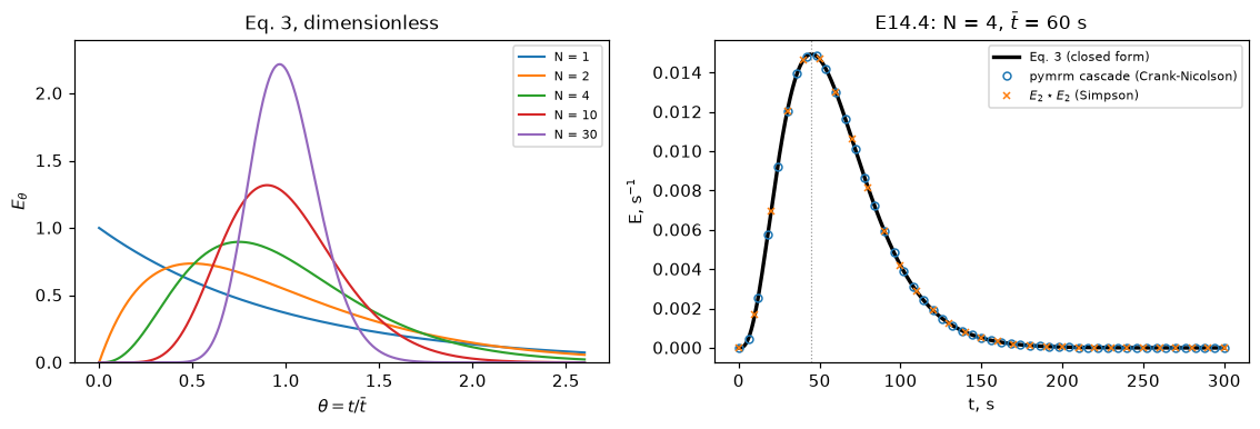
At the production time step (\(n_t = 4000\) over 300 s) the pymrm cascade reproduces Eq. 3 to 3.65e-08 s⁻¹, against a peak of 0.01494 s⁻¹. Refining the step: Crank-Nicolson at observed order 2.000, implicit Euler at 0.988 — both the expected values, and the check is on the step because the cell count is the model. The area under the pymrm curve falls 3.20e-06 short of 1 with no normalisation applied anywhere - the injected amount is one mole into \(V_1\) and \(E = uC_N\) throughout - and 3.20e-06 of that is the analytic tail of Eq. 3 beyond \(t = 300\) s, leaving 8.7e-11 that the march is responsible for.
The convolution route \(E_2\star E_2\) lands on the same curve to 6.9e-18 — and it does so on 2000 panels and on 20 panels alike (8.7e-18), which is the tell. For equal tank sizes the integrand is a cubic in \(s\) times a constant, Simpson integrates cubics exactly, and this number is therefore a structural identity, not an independent measurement: it checks the transcription of Eq. 3 and the plumbing of convolve_E, and it bounds nothing about the quadrature error on the unequal chains that the next two sections actually integrate. It is labelled structural in the coverage map for that reason, and the page’s independent route to the RTD is the Crank-Nicolson march against Eq. 3 above (3.65e-08).
5. Additivity, and the assumption it hides
Eq. 4 is a structural claim: for equal tanks it is the statement that a Gamma distribution convolved with a Gamma distribution of the same scale is a Gamma distribution, and the check below closes to round-off because it must. Reporting that as evidence would be exactly the “check that cannot fail”.
What the check can do is show what Eq. 4’s parenthesis — “(all of the same size)” — is worth. The means and variances of two unequal blocks still add: that is true of any two independent stages and has nothing to do with tanks in series. The shape does not follow. Below, two blocks with different tank sizes are convolved, and the result is compared with the tanks-in-series curve carrying the same mean and the same variance.
TI = TB4 / N4
# The window has to hold essentially the whole composite before the moment
# integrals below mean anything: the composite has tbar = 80 s, and a 340 s
# window truncates enough tail to dominate them (measured in the table below).
EQ4_WINDOW, EQ4_NPTS = 800.0, 331
_t = np.linspace(1e-9, EQ4_WINDOW, EQ4_NPTS)

# (a) equal tanks: structural, closes to round-off
EQ4_EQUAL = float(np.max(np.abs(convolve_E(_t, 2, 3, TI, TI) - E_time(_t, 5, 5 * TI))))

# (b) unequal blocks: 2 tanks of 10 s followed by 3 tanks of 20 s
tA, tB, MA, MB = 10.0, 20.0, 2, 3
CONV_UNEQ = convolve_E(_t, MA, MB, tA, tB)
MEAN_UNEQ = MA * tA + MB * tB
VAR_UNEQ = MA * tA ** 2 + MB * tB ** 2
N_MOMENT = MEAN_UNEQ ** 2 / VAR_UNEQ


def eq4_moment_devs(window, npts):
    """The two moment integrals on a given outer limit of the quadrature."""
    t = np.linspace(1e-9, window, npts)
    c = convolve_E(t, MA, MB, tA, tB)
    h = t[1] - t[0]
    sq = lambda y: h / 3.0 * (y[0] + y[-1] + 4 * y[1:-1:2].sum() + 2 * y[2:-1:2].sum())
    m = sq(t * c) / sq(c)
    v = sq((t - m) ** 2 * c) / sq(c)
    return abs(m - MEAN_UNEQ) / MEAN_UNEQ, abs(v - VAR_UNEQ) / VAR_UNEQ


EQ4_WIN = pd.DataFrame(
    [dict(window_s=w, npts=n, mean_reldev=eq4_moment_devs(w, n)[0],
          var_reldev=eq4_moment_devs(w, n)[1])
     for w, n in [(340.0, 141), (500.0, 207), (EQ4_WINDOW, EQ4_NPTS), (1200.0, 495)]])
EQ4_MEAN_DEV, EQ4_VAR_DEV = eq4_moment_devs(EQ4_WINDOW, EQ4_NPTS)
EQ4_MEAN_DEV_SHORT = float(EQ4_WIN.mean_reldev.iloc[0])
EQ4_VAR_DEV_SHORT = float(EQ4_WIN.var_reldev.iloc[0])

# The shape gap is an EXTREMUM, so it is bracketed and refined, not sampled.
_gap_fn = lambda t: abs(float(convolve_E(np.array([t]), MA, MB, tA, tB)[0])
                        - float(E_time(t, N_MOMENT, MEAN_UNEQ)))
CONV_UNEQ_PEAK = max_brent(
    lambda t: float(convolve_E(np.array([t]), MA, MB, tA, tB)[0]), 1e-9, EQ4_WINDOW)
EQ4_UNEQUAL_GAP = max_brent(_gap_fn, 1e-9, EQ4_WINDOW) / CONV_UNEQ_PEAK
EQ4_UNEQUAL_GAP_SAMPLED = float(np.max(np.abs(CONV_UNEQ - E_time(_t, N_MOMENT, MEAN_UNEQ)))
                                / CONV_UNEQ.max())

display(EQ4_WIN.round(10))
display(Markdown(f"""
**Equal tanks.** $E_2\\star E_3$ against $E_5$ with the same $\\bar t_i$:
**{EQ4_EQUAL:.2e}** s⁻¹. This is an identity and is labelled as one; it cannot
fail and it is not evidence for anything physical. It does not protect the
quadrature either: for equal tank sizes the integrand is a cubic and Simpson is
exact on cubics, which is why the same number comes back on 20 panels. The
quadrature is instead pinned by refining it directly, on the *unequal* integrand
where it is not exact.

**Unequal blocks.** {MA} tanks of {tA:g} s followed by {MB} tanks of {tB:g} s.
The first two moments of the composite are $\\sum t_i = {MEAN_UNEQ:g}$ s and
$\\sum t_i^2 = {VAR_UNEQ:g}$ s², and they add for *any* independent stages, exactly,
by a one-line argument — so the two deviations in the table above measure
**the outer limit of the quadrature and nothing else**. That is worth showing
rather than hiding: on the 340 s window a reader would see {EQ4_MEAN_DEV_SHORT:.1e}
and {EQ4_VAR_DEV_SHORT:.1e} and might take them for a test of additivity, whereas
they are the truncated tail of a distribution with $\\bar t = {MEAN_UNEQ:g}$ s. On
the {EQ4_WINDOW:g} s window used here they fall to {EQ4_MEAN_DEV:.1e} and
{EQ4_VAR_DEV:.1e}, and they stay there.

The *shape* is the part that can fail. The moment-matched tanks-in-series curve
($N = {N_MOMENT:.4f}$, $\\bar t = {MEAN_UNEQ:g}$ s) misses the true composite by
**{EQ4_UNEQUAL_GAP * 100:.4f} %** of its peak — bracketed and refined with
Brent's method rather than read off the plotting grid, which would have given
{EQ4_UNEQUAL_GAP_SAMPLED * 100:.4f} %. Eq. 4's parenthesis is doing work.
"""))| window_s | npts | mean_reldev | var_reldev | |
|---|---|---|---|---|
| 0 | 340.0 | 141 | 7.569460e-05 | 1.210169e-03 |
| 1 | 500.0 | 207 | 2.110000e-08 | 2.526700e-06 |
| 2 | 800.0 | 331 | 6.720000e-08 | 2.939000e-07 |
| 3 | 1200.0 | 495 | 6.810000e-08 | 2.974000e-07 |
Equal tanks. \(E_2\star E_3\) against \(E_5\) with the same \(\bar t_i\): 6.94e-18 s⁻¹. This is an identity and is labelled as one; it cannot fail and it is not evidence for anything physical. It does not protect the quadrature either: for equal tank sizes the integrand is a cubic and Simpson is exact on cubics, which is why the same number comes back on 20 panels. The quadrature is instead pinned by refining it directly, on the unequal integrand where it is not exact.
Unequal blocks. 2 tanks of 10 s followed by 3 tanks of 20 s. The first two moments of the composite are \(\sum t_i = 80\) s and \(\sum t_i^2 = 1400\) s², and they add for any independent stages, exactly, by a one-line argument — so the two deviations in the table above measure the outer limit of the quadrature and nothing else. That is worth showing rather than hiding: on the 340 s window a reader would see 7.6e-05 and 1.2e-03 and might take them for a test of additivity, whereas they are the truncated tail of a distribution with \(\bar t = 80\) s. On the 800 s window used here they fall to 6.7e-08 and 2.9e-07, and they stay there.
The shape is the part that can fail. The moment-matched tanks-in-series curve (\(N = 4.5714\), \(\bar t = 80\) s) misses the true composite by 1.8483 % of its peak — bracketed and refined with Brent’s method rather than read off the plotting grid, which would have given 1.8479 %. Eq. 4’s parenthesis is doing work.
6. Conversion: what the fitted \(N\) predicts
Everything in this section is held out of the E14.4 fit, which used two moments and nothing else. Three routes to the first-order exit concentration, sharing no code:
- pymrm — one sparse factorisation of the cascade with a linear sink;
- Eq. 9 — \(\left(1+k\bar t/N\right)^{-N}\);
- Eq. 11 — the macrofluid integral \(\int_0^\infty e^{-kt}E(t)\,dt\) by Simpson quadrature, which is the Laplace transform of Eq. 3 computed numerically.
For a first-order reaction the last two must agree, because Levenspiel writes “These equations apply to both micro- and macrofluids” — micromixing cannot matter when the rate is linear — so route 3 is a real test of Eq. 11’s transcription, of the assumed \(\bar t^{\,N}\) denominator, and of the quadrature, against an algebraic answer none of them can see.
Second order splits the two: Eq. 10’s nest of radicals is the microfluid, Eq. 11 with the batch solution \(C_0/(1+kC_0t)\) is the macrofluid, and they are different numbers.
KTS = np.array([0.25, 0.5, 1.0, 2.0, 5.0, 10.0])
NN = [1, 2, 3, 4, 6, 10, 20, 40]

rows = []
for N in NN:
    for kt in KTS:
        pym, _ = Cascade(N, tbar=1.0, c_in=1.0).first_order(kt)
        alg = eq9(N, kt)
        mac = eq11(N, 1.0, lambda t, kk=kt: np.exp(-kk * t))
        rows.append(dict(N=N, ktbar=kt, pymrm=pym, eq9=alg, eq11=mac))
FO = pd.DataFrame(rows)
FO["pymrm_dev"] = (FO.pymrm - FO.eq9).abs()
FO["eq11_dev"] = (FO.eq11 - FO.eq9).abs()
PYMRM_EQ9_DEV = float(FO.pymrm_dev.max())
EQ11_EQ9_DEV = float(FO.eq11_dev.max())
EQ11_NORM_DEV = max(abs(eq11(N, 1.0, lambda t: np.ones_like(t)) - 1.0) for N in NN)

# Simpson refinement of Eq. 11 - the quadrature IS the refinable axis here
_pans = np.array([2500, 5000, 10000, 20000])
_qerr = np.array([abs(eq11(4, 1.0, lambda t: np.exp(-2.0 * t), npanel=p) - eq9(4, 2.0))
                  for p in _pans])
EQ11_QUAD_ORDER = float(np.polyfit(np.log(1.0 / _pans), np.log(_qerr), 1)[0])

# second order: pymrm Newton vs Eq. 10, and macro vs micro
rows = []
for N in NN:
    for kt in KTS:
        pym, _, sol = Cascade(N, tbar=1.0, c_in=1.0).order_n(kt, order=2.0)
        alg = eq10(N, kt, 1.0 / N, 1.0)
        mac = eq11(N, 1.0, lambda t, kk=kt: 1.0 / (1.0 + kk * t))
        rows.append(dict(N=N, kC0tbar=kt, pymrm=pym, eq10=alg, eq11_macro=mac,
                         nit=sol.nit))
SO = pd.DataFrame(rows)
SO["pymrm_dev"] = (SO.pymrm - SO.eq10).abs()
SO["macro_micro_gap"] = ((SO.eq11_macro - SO.eq10) / SO.eq10).abs()
PYMRM_EQ10_DEV = float(SO.pymrm_dev.max())
MACRO_MICRO_MAX = float(SO.macro_micro_gap.max())
MACRO_MICRO_ROW = SO.loc[SO.macro_micro_gap.idxmax()]
NEWTON_MAX_IT = int(SO.nit.max())

# the printed small-deviation asymptote, for equal volume
ASYM_NS = np.array([10, 20, 40, 80, 160, 320])
_kt = 1.0
_asym_err = np.array([abs((eq9(n, _kt) / np.exp(-_kt) - 1.0) / (_kt ** 2 / (2 * n)) - 1.0)
                      for n in ASYM_NS])
ASYM_ORDER = float(-np.polyfit(np.log(ASYM_NS), np.log(_asym_err), 1)[0])
ASYM_DEV_N320 = float(_asym_err[-1])

display(Markdown(f"""
**First order, three routes.** Over {len(NN)} values of $N$ and
{len(KTS)} values of $k\\bar t$ (to $k\\bar t = {KTS.max():g}$):
pymrm against Eq. 9 to **{PYMRM_EQ9_DEV:.1e}**, and the Eq. 11 macrofluid
quadrature against Eq. 9 to **{EQ11_EQ9_DEV:.1e}**. Eq. 11 with a batch solution
of 1 integrates to 1 to **{EQ11_NORM_DEV:.1e}**, which is the check that fixes the
$\\bar t^{{\\,N}}$ reading of its denominator. The Simpson error falls at observed
order **{EQ11_QUAD_ORDER:.2f}**.

**Second order.** pymrm's Newton solve (pointwise `NumJac`, at most
{NEWTON_MAX_IT} iterations) against Eq. 10's nest of $N$ radicals to
**{PYMRM_EQ10_DEV:.1e}**. Micro- and macrofluid are *not* the same here: the gap
reaches **{MACRO_MICRO_MAX * 100:.2f} %** at $N = {int(MACRO_MICRO_ROW.N)}$,
$kC_0\\bar t = {MACRO_MICRO_ROW.kC0tbar:g}$, and it is the macrofluid that converts
further. This is the same statement [`A2.8`](../A2.8-zwietering-segregation/)
makes with bounds; here it is the two specific states Levenspiel prints.

**The printed asymptote.** $C_{{A,N}}/C_{{Ap}} = 1 + (k\\bar t)^2/(2N)$ for the same
volume: the relative error of that expression falls at observed order
**{ASYM_ORDER:.2f}** in $N$ and is {ASYM_DEV_N320:.2e} at $N = {ASYM_NS[-1]}$, so the
printed formula is the correct first term. Its printed companion for the same
final conversion is *not*; see the next section.
"""))
First order, three routes. Over 8 values of \(N\) and 6 values of \(k\bar t\) (to \(k\bar t = 10\)): pymrm against Eq. 9 to 2.4e-15, and the Eq. 11 macrofluid quadrature against Eq. 9 to 1.5e-10. Eq. 11 with a batch solution of 1 integrates to 1 to 2.3e-11, which is the check that fixes the \(\bar t^{\,N}\) reading of its denominator. The Simpson error falls at observed order 3.98.
Second order. pymrm’s Newton solve (pointwise NumJac, at most 8 iterations) against Eq. 10’s nest of \(N\) radicals to 3.2e-14. Micro- and macrofluid are not the same here: the gap reaches 25.43 % at \(N = 1\), \(kC_0\bar t = 10\), and it is the macrofluid that converts further. This is the same statement A2.8 makes with bounds; here it is the two specific states Levenspiel prints.
The printed asymptote. \(C_{A,N}/C_{Ap} = 1 + (k\bar t)^2/(2N)\) for the same volume: the relative error of that expression falls at observed order 0.99 in \(N\) and is 1.30e-03 at \(N = 320\), so the printed formula is the correct first term. Its printed companion for the same final conversion is not; see the next section.
7. Printed defects
Six items are wrong or ambiguous as printed — five defects and one typesetting ambiguity. Each is established from the book’s own numbers, and none is repaired in the transcription: the CSV carries the glyphs as they appear and this section says what they should be.
The first of them is the most consequential, because it is a modelling rule and not a unit or a tick label: a reader who applies it gets a different reactor.
# (0) Fig. 14.7's dispersion-conversion rule, inverted. Everything here is
# arithmetic on printed values; the COST of the inversion is measured in
# section 9, where a dispersion solve exists.
HALF = P("Fig14.7", "dispersion_rule_half")
N_SYM = P("Fig14.7", "N_symmetric_threshold")
SIG_COEF = P("Fig13.12", "sigma2_theta_over_DuL") # sigma^2_theta = 2 (D/uL)
DUL_LIMIT = P("Fig13.11", "DuL_small_deviation_limit")
# Ch. 13's variance with Ch. 14's 1/N: 1/N = SIG_COEF (D/uL) -> N = (1/SIG_COEF)(uL/D)
DEFECT_FIG147_FROM_CH13 = abs(1.0 / SIG_COEF - HALF)
# the annotation's own threshold, pushed through the CORRECT rule
DEFECT_FIG147_THRESHOLD_DUL = HALF / N_SYM
DEFECT_FIG147_THRESHOLD_DEV = abs(DEFECT_FIG147_THRESHOLD_DUL - DUL_LIMIT)
# ... and through the rule AS PRINTED
DEFECT_FIG147_THRESHOLD_DUL_PRINTED = N_SYM / HALF
# (1) the factor of two in "for same C_A,final".
# The quantity is a LIMIT, x -> 0, of (V_N/V_p - 1)/x with x = k tbar_i, so it is
# extrapolated rather than fitted over an arbitrary window: a polyfit on a finite
# window returns 2.0003 or 2.03 depending only on how wide the window is, and the
# trailing digits would then be pinned in CI while meaning nothing.
def _vslope(x):
"""(V_N/V_p - 1)/x from the book's own Eq. 9 against plug flow."""
return (x / np.log1p(x) - 1.0) / x
DEFECT_SLOPE_TABLE = pd.DataFrame(
[dict(x=x, raw=_vslope(x), richardson=2 * _vslope(x / 2) - _vslope(x),
polyfit_ratio=1.0 / float(np.polyfit(np.linspace(1e-6, x, 400),
np.linspace(1e-6, x, 400)
/ np.log1p(np.linspace(1e-6, x, 400)) - 1.0,
1)[0]))
for x in [4e-1, 4e-2, 4e-3, 4e-4]])
DEFECT_EXACT_SLOPE = float(2 * _vslope(5e-5) - _vslope(1e-4)) # -> 1/2 - x^2/48
DEFECT_MID_SLOPE = 1.0 # "1 + k tbar_i" -> slope 1
DEFECT_RIGHT_SLOPE = 0.5 # "1 + k tbar/(2N)" -> slope 1/2
DEFECT_FACTOR = DEFECT_MID_SLOPE / DEFECT_EXACT_SLOPE
DEFECT_RIGHT_RATIO = DEFECT_RIGHT_SLOPE / DEFECT_EXACT_SLOPE
# direct numerical confirmation at a finite N: what volume ratio does Eq. 9 need?
_N, _ktb = 20, 1.0
_target = np.exp(-_ktb) # plug-flow conversion at k tbar = 1
_ratio = brentq(lambda r: eq9(_N, _ktb * r) - _target, 1.0, 5.0, xtol=1e-14)
DEFECT_RATIO_TRUE = _ratio
DEFECT_RATIO_MID = 1.0 + _ktb / _N
DEFECT_RATIO_RIGHT = 1.0 + _ktb / (2 * _N)
# (2) Eq. 11's denominator: tbar_N (subscript) against tbar**N (superscript)
_N11, _tb11 = 4, 60.0
NORM_SUPER = eq11(_N11, _tb11, lambda t: np.ones_like(t))
NORM_SUB = NORM_SUPER * _tb11 ** _N11 / _tb11 # what the subscript reading gives
DEFECT_EQ11_NORM_SUB = NORM_SUB
# (3) Fig. E14.4b's axis tick, against the peak of the curve AS PRINTED
DEFECT_TICK_RATIO = TICK_P / E144_EMAX_PRINTED
# (4) E14.2's "moles"; (5) E14.4's "900 s"
DEFECT_VAR_UNIT_VALUE_DEV = abs(DV - DV_P) # the VALUE is right; the unit is not
display(DEFECT_SLOPE_TABLE.round(10))
display(Markdown(f"""
**(a) Fig. 14.7, book p. 327 — the dispersion-conversion rule is inverted.**
Inside the axes box: *"When $N > {N_SYM:g}$ the curve becomes symmetrical in which
case use fig. 13-11 with $N = {HALF:g}(\\mathbf{{D}}/uL)$"*. The ratio is upside
down, and the book supplies the proof twice over.
*From its own variance.* Chapter 13 prints
$\\sigma^2_\\theta = {SIG_COEF:g}(\\mathbf{{D}}/uL)$ (Fig. 13.12, book p. 303) and
Chapter 14 prints $\\sigma^2_\\theta = 1/N$ (Eq. 3). Together they give
$N = (1/{SIG_COEF:g})(uL/\\mathbf{{D}})$, whose coefficient matches the printed
{HALF:g} to **{DEFECT_FIG147_FROM_CH13:.0e}** — on the *reciprocal* ratio.
*From its own threshold.* Pushed through the corrected rule, the annotation's
$N > {N_SYM:g}$ is $\\mathbf{{D}}/uL < {DEFECT_FIG147_THRESHOLD_DUL:g}$, and
"Small Deviation from Plug Flow, $\\mathbf{{D}}/uL < {DUL_LIMIT:g}$" is the printed
heading of the section that owns Fig. 13.11: the two agree to
**{DEFECT_FIG147_THRESHOLD_DEV:.0e}**. As printed, the same threshold would send
the reader to $\\mathbf{{D}}/uL > {DEFECT_FIG147_THRESHOLD_DUL_PRINTED:g}$, off a
figure drawn between 0.00005 and 0.0128 and at the opposite end of the flow
regime. Section 9 measures what that costs in conversion.
**(b) Section 14.2, book p. 328 — a factor of two.** The line reads
$V_{{N\\,\\text{{tanks}}}}/V_p = 1 + k\\bar t_i = 1 + k\\bar t/(2N)$. With the book's own
$\\bar t = N\\bar t_i$ those two right-hand sides differ by exactly two. Expanding the
book's own Eq. 9 against plug flow gives $V_N/V_p = x/\\ln(1+x)$ with
$x = k\\bar t_i$, whose leading correction has slope
**{DEFECT_EXACT_SLOPE:.9f}** — the table above extrapolates it to $x = 0$
instead of fitting it, because the `raw` and `polyfit_ratio` columns show that a
finite window puts spurious digits on an exactly rational number. Against that,
the middle expression has slope {DEFECT_MID_SLOPE:g} (a factor
**{DEFECT_FACTOR:.9f}** too large, i.e. exactly two) and the right-hand one
{DEFECT_RIGHT_SLOPE:g} (factor {DEFECT_RIGHT_RATIO:.9f}, i.e. exactly one). At
$N = {_N}$, $k\\bar t = {_ktb:g}$ the volume ratio that Eq. 9 actually needs is
**{DEFECT_RATIO_TRUE:.6f}**, against {DEFECT_RATIO_MID:.6f} from the middle form
and {DEFECT_RATIO_RIGHT:.6f} from the right-hand one. **The middle expression is
missing a factor of $\\tfrac12$**; the right-hand form, and the companion
equal-volume formula $1+(k\\bar t)^2/(2N)$, are correct as printed. Reported, not
repaired.
**(c) Eq. 11, book p. 329 — a subscript where a superscript belongs.** The
prefactor denominator is set as $(N-1)!\\,\\bar t_N$ with $N$ lowered. With
$\\bar t^{{\\,N}}$ the kernel integrates to {NORM_SUPER:.10f}; with the printed
$\\bar t_N = \\bar t$ it integrates to {DEFECT_EQ11_NORM_SUB:.4g} at $N = {_N11}$,
$\\bar t = {_tb11:g}$ s — not dimensionless, let alone normalised. The book itself
prints the raised form two pages later in E14.4
($\\mathbf{{E}} = t^{{N-1}}/\\bar t^{{\\,N}}\\cdot N^N/(N-1)!\\cdot e^{{-tN/\\bar t}}$), which
settles the reading. A typesetting slip, not a modelling one.
**(d) Fig. E14.4b, book p. 334 — a transposed digit.** The top axis tick is
labelled {TICK_P:g} s⁻¹, on an axis whose other ticks are 0, 0.005 and 0.010 at
equal spacing. The book's own printed $E(t) = {PRE_P:.4e}\\,t^3e^{{-{EXP_P:g}t}}$
peaks at $t = {E144_TMAX_PRINTED:.6g}$ s with $E = {E144_EMAX_PRINTED:.7g}$ s⁻¹, so
the tick is {DEFECT_TICK_RATIO:.2f}$\\times$ the whole curve. It should read 0.015.
(Note which curve: with the *unrounded* coefficients the peak is
{E144_EMAX:.7g} s⁻¹ and the ratio {TICK_P / E144_EMAX:.2f}. The tick belongs to the
printed curve, so the printed coefficients are the ones used here.)
**(e) E14.2, book p. 331 — "$L = 272$ moles".** The quantity is a distance along
the Ohio River. The Comment two lines below reads "any location where
$L \\le 272$ **miles** is suspect", and every input to the calculation is in miles.
The *value* {E142_L_P:g} is exactly right, as the reproduction above shows; only
the unit is a slip.
**(f) E14.4, book p. 333 — "$\\Delta(\\sigma^2) = 1000 - 100 = 900$ s".** The same
class of slip as (e), in the same chapter: a variance carrying the unit of a
time. The inputs two lines above are read off Fig. E14.4a as {V_IN:g} s² and
{V_OUT:g} s², and the very next line divides $(\\Delta\\bar t)^2$ by this quantity to
get a dimensionless tank count, which only works in s². The *value* {DV_P:g} is
right — the reproduction above matches it to {DEFECT_VAR_UNIT_VALUE_DEV:.0e}
— and the CSV's `note` column carries the correction while `printed_as`
carries the glyphs.
"""))| x | raw | richardson | polyfit_ratio | |
|---|---|---|---|---|
| 0 | 0.4000 | 0.472013 | 0.497616 | 2.120493 |
| 1 | 0.0400 | 0.496732 | 0.499968 | 2.013185 |
| 2 | 0.0040 | 0.499667 | 0.500000 | 2.001332 |
| 3 | 0.0004 | 0.499967 | 0.500000 | 2.000134 |
(a) Fig. 14.7, book p. 327 — the dispersion-conversion rule is inverted. Inside the axes box: “When \(N > 50\) the curve becomes symmetrical in which case use fig. 13-11 with \(N = 0.5(\mathbf{D}/uL)\)”. The ratio is upside down, and the book supplies the proof twice over.
From its own variance. Chapter 13 prints \(\sigma^2_\theta = 2(\mathbf{D}/uL)\) (Fig. 13.12, book p. 303) and Chapter 14 prints \(\sigma^2_\theta = 1/N\) (Eq. 3). Together they give \(N = (1/2)(uL/\mathbf{D})\), whose coefficient matches the printed 0.5 to 0e+00 — on the reciprocal ratio.
From its own threshold. Pushed through the corrected rule, the annotation’s \(N > 50\) is \(\mathbf{D}/uL < 0.01\), and “Small Deviation from Plug Flow, \(\mathbf{D}/uL < 0.01\)” is the printed heading of the section that owns Fig. 13.11: the two agree to 0e+00. As printed, the same threshold would send the reader to \(\mathbf{D}/uL > 100\), off a figure drawn between 0.00005 and 0.0128 and at the opposite end of the flow regime. Section 9 measures what that costs in conversion.
(b) Section 14.2, book p. 328 — a factor of two. The line reads \(V_{N\,\text{tanks}}/V_p = 1 + k\bar t_i = 1 + k\bar t/(2N)\). With the book’s own \(\bar t = N\bar t_i\) those two right-hand sides differ by exactly two. Expanding the book’s own Eq. 9 against plug flow gives \(V_N/V_p = x/\ln(1+x)\) with \(x = k\bar t_i\), whose leading correction has slope 0.500000000 — the table above extrapolates it to \(x = 0\) instead of fitting it, because the raw and polyfit_ratio columns show that a finite window puts spurious digits on an exactly rational number. Against that, the middle expression has slope 1 (a factor 2.000000001 too large, i.e. exactly two) and the right-hand one 0.5 (factor 1.000000000, i.e. exactly one). At \(N = 20\), \(k\bar t = 1\) the volume ratio that Eq. 9 actually needs is 1.025422, against 1.050000 from the middle form and 1.025000 from the right-hand one. The middle expression is missing a factor of \(\tfrac12\); the right-hand form, and the companion equal-volume formula \(1+(k\bar t)^2/(2N)\), are correct as printed. Reported, not repaired.
(c) Eq. 11, book p. 329 — a subscript where a superscript belongs. The prefactor denominator is set as \((N-1)!\,\bar t_N\) with \(N\) lowered. With \(\bar t^{\,N}\) the kernel integrates to 1.0000000000; with the printed \(\bar t_N = \bar t\) it integrates to 2.16e+05 at \(N = 4\), \(\bar t = 60\) s — not dimensionless, let alone normalised. The book itself prints the raised form two pages later in E14.4 (\(\mathbf{E} = t^{N-1}/\bar t^{\,N}\cdot N^N/(N-1)!\cdot e^{-tN/\bar t}\)), which settles the reading. A typesetting slip, not a modelling one.
(d) Fig. E14.4b, book p. 334 — a transposed digit. The top axis tick is labelled 0.105 s⁻¹, on an axis whose other ticks are 0, 0.005 and 0.010 at equal spacing. The book’s own printed \(E(t) = 3.2922e-06\,t^3e^{-0.0667t}\) peaks at \(t = 44.9775\) s with \(E = 0.01491382\) s⁻¹, so the tick is 7.04\(\times\) the whole curve. It should read 0.015. (Note which curve: with the unrounded coefficients the peak is 0.01493612 s⁻¹ and the ratio 7.03. The tick belongs to the printed curve, so the printed coefficients are the ones used here.)
(e) E14.2, book p. 331 — “\(L = 272\) moles”. The quantity is a distance along the Ohio River. The Comment two lines below reads “any location where \(L \le 272\) miles is suspect”, and every input to the calculation is in miles. The value 272 is exactly right, as the reproduction above shows; only the unit is a slip.
(f) E14.4, book p. 333 — “\(\Delta(\sigma^2) = 1000 - 100 = 900\) s”. The same class of slip as (e), in the same chapter: a variance carrying the unit of a time. The inputs two lines above are read off Fig. E14.4a as 100 s² and 1000 s², and the very next line divides \((\Delta\bar t)^2\) by this quantity to get a dimensionless tank count, which only works in s². The value 900 is right — the reproduction above matches it to 0e+00 — and the CSV’s note column carries the correction while printed_as carries the glyphs.
8. What two moments cannot buy: the headline
E14.4 uses exactly two numbers, \(\Delta\bar t\) and \(\Delta(\sigma^2)\), and returns “4 tanks”. The method assumes the vessel is \(N\) equal tanks; with two moments there is no way to check that assumption, because a chain of unequal tanks has the same two moments as some equal chain by construction.
Here is a specific alternative. A five-stage chain with residence times \(9, 9, 9, 9, 24\) s has
\[\sum t_i = 60\ \text{s} = \Delta\bar t,\qquad \sum t_i^2 = 4(81) + 576 = 900\ \text{s}^2 = \Delta(\sigma^2),\]
exactly the two numbers E14.4 measured — the same mean, the same variance, to the last digit. It is therefore indistinguishable from Levenspiel’s four equal tanks by his own method, and every gallery page that reuses a fitted \(N\) inherits the ambiguity. It is also admissible: E14.3’s own Figs. E14.3b–d (book p. 333) work with \(V_1 = \tfrac13\), \(V_2 = \tfrac23\) and with \(N_1 = 12\), \(N_2 = 24\), so unequal blocks are not excluded by the chapter. And it is the natural choice — 9, 9, 9, 9, 24 is the second root of \(a^2 - 24a + 135 = 0\), i.e. the only non-equal member of the four-equal-plus-one family.
Three things have to be said carefully about the number that comes out, because each of them is a way of overstating it:
- it is a gap in outlet concentration, which is not the same as a gap in conversion, and both are printed below;
- it is the value at the right-hand edge of the range swept, and it is monotone in \(k\bar t\), so the sweep is extended past that edge rather than stopped at it;
- it is one chain, so it is a lower bound on what two moments leave open. The upper bound over the whole family is computed in closed form afterwards.
Both chains are built with the same Cascade class, differing only in faces.
T_EQ = np.full(4, 15.0)
T_UN = np.array([9.0, 9.0, 9.0, 9.0, 24.0])
assert np.isclose(T_UN.sum(), DTB) and np.isclose((T_UN ** 2).sum(), DV), "moments must match exactly"
AMBIG_MEAN_DEV = abs(T_UN.sum() - T_EQ.sum())
AMBIG_VAR_DEV = abs((T_UN ** 2).sum() - (T_EQ ** 2).sum())


def chain(ts, tbar_total):
    """A Cascade whose cells are sized in proportion to the given residence times."""
    faces = np.concatenate([[0.0], np.cumsum(ts) / ts.sum()])
    return Cascade(len(ts), tbar=tbar_total, c_in=1.0, faces=faces)


rows = []
for kt in [0.5, 1.0, 2.0, 5.0, 10.0, 20.0, 50.0]:
    k = kt / DTB
    a1, _ = chain(T_EQ, DTB).first_order(k)
    b1, _ = chain(T_UN, DTB).first_order(k)
    a2, _, _ = chain(T_EQ, DTB).order_n(k, order=2.0)
    b2, _, _ = chain(T_UN, DTB).order_n(k, order=2.0)
    rows.append(dict(ktbar=kt, eq_first=a1, un_first=b1,
                     conc_gap=abs(b1 - a1) / a1,
                     eq_conv=1.0 - a1, un_conv=1.0 - b1,
                     conv_gap=abs((1.0 - b1) - (1.0 - a1)) / (1.0 - a1),
                     eq_second=a2, un_second=b2, second_gap=abs(b2 - a2) / a2))
AMB = pd.DataFrame(rows)
AMBIG_KT_HEADLINE = 10.0                      # the right-hand edge of the ORIGINAL sweep
_hl = AMB.loc[AMB.ktbar == AMBIG_KT_HEADLINE].iloc[0]
AMBIG_FIRST_MAX = float(_hl.conc_gap)         # the 5-stage chain AT k tbar = 10
AMBIG_FIRST_MAX_SWEPT = float(AMB.conc_gap.max())      # ... and at the new edge, 50
AMBIG_CONV_MAX = float(AMB.conv_gap.max())    # the same thing in CONVERSION
AMBIG_CONV_KT = float(AMB.loc[AMB.conv_gap.idxmax(), "ktbar"])
AMBIG_CONV_HL = float(_hl.conv_gap)
AMBIG_SECOND_MAX = float(AMB.loc[AMB.ktbar == AMBIG_KT_HEADLINE, "second_gap"].iloc[0])
AMBIG_FIRST_KT2 = float(AMB.loc[AMB.ktbar == 2.0, "conc_gap"].iloc[0])
# the pymrm unequal chain against the product formula it must satisfy
_k = 2.0 / DTB
_prod = 1.0 / np.prod(1.0 + _k * T_UN)
AMBIG_PYMRM_DEV = abs(chain(T_UN, DTB).first_order(_k)[0] - _prod)

_t = np.linspace(1e-9, 260.0, 400)
E_UN = convolve_E(_t, 4, 1, 9.0, 24.0)
# the RTD gap is an extremum too: bracketed and refined, and the denominator is
# the root-found peak of Eq. 3 at N = 4, tbar = 60 s computed in section 2.
AMBIG_RTD_GAP = max_brent(
    lambda t: abs(float(convolve_E(np.array([t]), 4, 1, 9.0, 24.0)[0])
                  - float(E_time(t, 4, DTB))), 1e-9, 260.0) / E144_EMAX

fig, ax = plt.subplots(1, 2, figsize=(10.4, 3.6))
ax[0].plot(_t, E_time(_t, N4, DTB), lw=2.0, label=r"4 equal tanks of 15 s (Levenspiel)")
ax[0].plot(_t, E_UN, lw=2.0, ls="--", label=r"5 tanks of 9,9,9,9,24 s")
ax[0].set_xlabel("t, s"); ax[0].set_ylabel(r"E, s$^{-1}$")
ax[0].set_title(r"same $\bar t$ = 60 s, same $\sigma^2$ = 900 s$^2$")
ax[0].legend(fontsize=7.5)
ax[1].semilogy(AMB.ktbar, AMB.conc_gap * 100, "o-", label="first order, exit concentration")
ax[1].semilogy(AMB.ktbar, AMB.second_gap * 100, "s--", label="second order, exit concentration")
ax[1].semilogy(AMB.ktbar, AMB.conv_gap * 100, "^:", label="first order, CONVERSION")
ax[1].set_xlabel(r"$k\bar t$  (or $kC_0\bar t$)")
ax[1].set_ylabel("relative difference, %")
ax[1].set_title("what the two-moment fit does not fix"); ax[1].legend(fontsize=7)
plt.tight_layout(); plt.show()
display(AMB.round(6))
display(Markdown(f"""
The two chains match E14.4's measured mean to **{AMBIG_MEAN_DEV:.0e}** s and its
measured variance to **{AMBIG_VAR_DEV:.0e}** s² — that is, exactly. Their exit
curves differ by **{AMBIG_RTD_GAP * 100:.1f} %** of the peak.

**In exit concentration** the two chains differ by
**{AMBIG_FIRST_MAX * 100:.1f} %** at $k\\bar t = {AMBIG_KT_HEADLINE:g}$, first order.
That is the number this page quotes, and the table shows what it is and is not:
it is monotone in $k\\bar t$, so it is not a maximum over the sweep but the value
at whichever $k\\bar t$ one stops at — {AMBIG_FIRST_KT2 * 100:.2f} % at
$k\\bar t = 2$, {AMB.conc_gap.iloc[-1] * 100:.1f} % at
$k\\bar t = {AMB.ktbar.iloc[-1]:g}$. Second order at
$k\\bar t = {AMBIG_KT_HEADLINE:g}$: {AMBIG_SECOND_MAX * 100:.1f} %.

**In conversion** it is a far smaller number, and saying "converts 23 %
differently" would be wrong. At $k\\bar t = {AMBIG_KT_HEADLINE:g}$ the two chains
convert {_hl.eq_conv * 100:.3f} % and {_hl.un_conv * 100:.3f} % —
{abs(_hl.un_conv - _hl.eq_conv) * 100:.2f} percentage points apart, or
{AMBIG_CONV_HL * 100:.2f} % relative — and over the whole sweep the relative gap in
conversion never exceeds **{AMBIG_CONV_MAX * 100:.2f} %**, at
$k\\bar t = {AMBIG_CONV_KT:g}$. The two statements are consistent: at high
$k\\bar t$ both chains convert almost everything, so a large relative difference in
what is *left* is a small difference in what is *converted*. Which of the two
matters is the reader's question, not the page's — for a purification duty,
or for anything sized on the outlet, it is the first.

The pymrm unequal chain reproduces the staged product $\\prod (1+kt_i)^{{-1}}$ to
{AMBIG_PYMRM_DEV:.1e}, so the difference is physics and not a solver artefact.

This is not a criticism of E14.4 — the method is exactly as good as its
inputs, and Levenspiel says plainly that the tanks are assumed equal. It is a
statement of what a two-moment fit is worth: **it fixes the RTD only within the
family it assumes, and the conversion it implies inherits that ambiguity.**
""" ))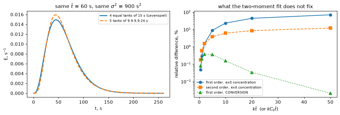
| ktbar | eq_first | un_first | conc_gap | eq_conv | un_conv | conv_gap | eq_second | un_second | second_gap | |
|---|---|---|---|---|---|---|---|---|---|---|
| 0 | 0.5 | 0.624295 | 0.624000 | 0.000472 | 0.375705 | 0.376000 | 0.000784 | 0.687166 | 0.685959 | 0.001756 |
| 1 | 1.0 | 0.409600 | 0.408395 | 0.002941 | 0.590400 | 0.591605 | 0.002041 | 0.538538 | 0.535271 | 0.006065 |
| 2 | 2.0 | 0.197531 | 0.194515 | 0.015266 | 0.802469 | 0.805485 | 0.003758 | 0.387588 | 0.381479 | 0.015761 |
| 3 | 5.0 | 0.039018 | 0.035541 | 0.089130 | 0.960982 | 0.964459 | 0.003619 | 0.224132 | 0.215546 | 0.038305 |
| 4 | 10.0 | 0.006664 | 0.005120 | 0.231680 | 0.993336 | 0.994880 | 0.001554 | 0.138903 | 0.130450 | 0.060852 |
| 5 | 20.0 | 0.000772 | 0.000434 | 0.437500 | 0.999228 | 0.999566 | 0.000338 | 0.082833 | 0.075740 | 0.085625 |
| 6 | 50.0 | 0.000030 | 0.000009 | 0.697002 | 0.999970 | 0.999991 | 0.000021 | 0.040156 | 0.035378 | 0.118977 |
The two chains match E14.4’s measured mean to 0e+00 s and its measured variance to 0e+00 s² — that is, exactly. Their exit curves differ by 6.9 % of the peak.
In exit concentration the two chains differ by 23.2 % at \(k\bar t = 10\), first order. That is the number this page quotes, and the table shows what it is and is not: it is monotone in \(k\bar t\), so it is not a maximum over the sweep but the value at whichever \(k\bar t\) one stops at — 1.53 % at \(k\bar t = 2\), 69.7 % at \(k\bar t = 50\). Second order at \(k\bar t = 10\): 6.1 %.
In conversion it is a far smaller number, and saying “converts 23 % differently” would be wrong. At \(k\bar t = 10\) the two chains convert 99.334 % and 99.488 % — 0.15 percentage points apart, or 0.16 % relative — and over the whole sweep the relative gap in conversion never exceeds 0.38 %, at \(k\bar t = 2\). The two statements are consistent: at high \(k\bar t\) both chains convert almost everything, so a large relative difference in what is left is a small difference in what is converted. Which of the two matters is the reader’s question, not the page’s — for a purification duty, or for anything sized on the outlet, it is the first.
The pymrm unequal chain reproduces the staged product \(\prod (1+kt_i)^{-1}\) to 8.3e-17, so the difference is physics and not a solver artefact.
This is not a criticism of E14.4 — the method is exactly as good as its inputs, and Levenspiel says plainly that the tanks are assumed equal. It is a statement of what a two-moment fit is worth: it fixes the RTD only within the family it assumes, and the conversion it implies inherits that ambiguity.
8b. The whole family, in closed form
One chain is an example. The honest question is the range of outlet concentrations consistent with \(\sum t_i = 60\) s and \(\sum t_i^2 = 900\) s², because that is the set of vessels E14.4’s two numbers cannot tell apart.
The answer is not a search. For a first-order reaction \(C/C_0 = \prod (1+kt_i)^{-1}\), so maximising the ambiguity means extremising \(\sum \ln(1+kt_i)\) under two linear-and-quadratic constraints. The Lagrange condition is \(k/(1+kt_i) = \lambda + 2\mu t_i\) for every \(i\), and that equation has at most two roots in \(t\): the left side is increasing and concave, the right side is a straight line. So every extremal chain consists of at most two distinct tank sizes, and the extremum can be enumerated over \((n, m)\) — \(m\) tanks of one size, \(n-m\) of another, with the two moments fixing both sizes in closed form.
The supremum itself is closed form. Write \(T = \sum t_i\), \(S = \sum t_i^2\), and note that \(t_i \le \sqrt S\) for every \(i\). With \(h(t) = \ln(1+kt) - kt\), the function \(h(t)/t^2\) is increasing on \(t>0\) (its numerator derivative reduces to \(u^2/(1+u)^2 \ge 0\) with \(u = kt\)), so \(h(t_i) \le h(\sqrt S)\,t_i^2/S\) for every \(i\), and summing gives
\[\sum \ln(1+kt_i)\ \le\ \ln\!\left(1+k\sqrt S\right) + k\left(T - \sqrt S\right),\]
with equality only when every \(t_i\) is \(0\) or \(\sqrt S\). The bound is therefore attained only in the limit of one tank of \(\sqrt S = 30\) s followed by plug flow of \(T - \sqrt S = 30\) s — a chain of infinitely many infinitesimal tanks. That is the most-converting vessel E14.4’s two numbers permit, and no chain reaches it.
T_MOM, S_MOM = float(DTB), float(DV) # the two numbers E14.4 measured
N_FAMILY_MAX = 400
def two_value_chains(n, m, T=T_MOM, S=S_MOM):
"""Residence times of a chain of m tanks of one size and n-m of another that
matches BOTH printed moments. Closed form: the constraints reduce to a
quadratic in the first size."""
p, q = m, n - m
A = p * q + p * p
B = -2.0 * T * p
C = T * T - q * S
disc = B * B - 4.0 * A * C
if disc < 0.0:
return []
out = []
for a in ((-B + np.sqrt(disc)) / (2.0 * A), (-B - np.sqrt(disc)) / (2.0 * A)):
b = (T - p * a) / q
if a > 0.0 and b > 0.0:
out.append(np.concatenate([np.full(p, a), np.full(q, b)]))
return out
def conc_of(ts, k):
"""prod (1 + k t_i)^-1, in logs so that 400-stage chains do not underflow."""
return float(np.exp(-np.sum(np.log1p(k * np.asarray(ts)))))
def family_sup(k, T=T_MOM, S=S_MOM):
"""The closed-form supremum of the conversion: one sqrt(S) tank + plug flow."""
return np.exp(-k * (T - np.sqrt(S))) / (1.0 + k * np.sqrt(S))
rows, FAM_CONV = [], {}
for kt in [2.0, AMBIG_KT_HEADLINE]:
k = kt / T_MOM
base = conc_of(T_EQ, k)
lo, hi, arg = base, base, None
conv = []
for n in range(5, N_FAMILY_MAX + 1):
best_n = 0.0
for m in range(1, n):
for ts in two_value_chains(n, m):
c = conc_of(ts, k)
if c < lo:
lo, arg = c, (n, m, ts[0], ts[-1])
hi = max(hi, c)
best_n = max(best_n, abs(c - base) / base)
if n in (5, 6, 8, 12, 40, 100, N_FAMILY_MAX):
conv.append(dict(stages=n, max_conc_gap=best_n))
sup = family_sup(k)
rows.append(dict(ktbar=kt, equal_chain=base,
most_converting=lo, least_converting=hi,
gap_below=abs(lo - base) / base, gap_above=abs(hi - base) / base,
closed_form_sup=sup, sup_gap=abs(sup - base) / base,
best_n=arg[0], best_a=arg[2], best_b=arg[3]))
FAM_CONV[kt] = pd.DataFrame(conv)
FAM = pd.DataFrame(rows)
# the closed form must BOUND every enumerated chain - asserted, not assumed
for _r in rows:
assert _r["most_converting"] >= family_sup(_r["ktbar"] / T_MOM) - 1e-14, _r
AMBIG_FAMILY_SUP_GAP = float(FAM.loc[FAM.ktbar == AMBIG_KT_HEADLINE, "sup_gap"].iloc[0])
AMBIG_FAMILY_SUP_GAP_KT2 = float(FAM.loc[FAM.ktbar == 2.0, "sup_gap"].iloc[0])
AMBIG_FAMILY_BEST_N = float(FAM.loc[FAM.ktbar == AMBIG_KT_HEADLINE,
"gap_below"].iloc[0])
AMBIG_FAMILY_ABOVE = float(FAM.gap_above.max())
display(FAM.round(8))
display(FAM_CONV[AMBIG_KT_HEADLINE].round(6))
display(Markdown(f"""
At $k\\bar t = {AMBIG_KT_HEADLINE:g}$ the five-stage chain's
{AMBIG_FIRST_MAX * 100:.1f} % is a **lower bound**. Enumerating every two-value
chain up to {N_FAMILY_MAX} stages reaches {AMBIG_FAMILY_BEST_N * 100:.1f} %, and the
closed-form supremum — one {np.sqrt(S_MOM):g} s tank followed by
{T_MOM - np.sqrt(S_MOM):g} s of plug flow — is
**{AMBIG_FAMILY_SUP_GAP * 100:.1f} %**. At $k\\bar t = 2$ the same three numbers are
{AMBIG_FIRST_KT2 * 100:.2f} %, {float(FAM.loc[FAM.ktbar == 2.0, "gap_below"].iloc[0]) * 100:.2f} %
and {AMBIG_FAMILY_SUP_GAP_KT2 * 100:.2f} %. The ambiguity is **one-sided**: the
enumeration finds no chain at all that converts *less* than four equal tanks
(largest gap in that direction, {AMBIG_FAMILY_ABOVE * 100:.2f} %). Four equal
tanks already sit at the smallest $\\sum t_i^2$ their stage count allows, so every
other admissible chain must put more residence time into one stage and split the
rest more finely — and the enumeration says that always converts further.
Levenspiel's answer is therefore the *least*-converting vessel consistent with
his own two numbers, which is the conservative end and worth knowing.
So the correct statement of the headline is: E14.4's two numbers pin the outlet
concentration only to within a factor of
{1.0 / (1.0 - AMBIG_FAMILY_SUP_GAP):.2f} at $k\\bar t = {AMBIG_KT_HEADLINE:g}$; the
9, 9, 9, 9, 24 s chain realises {AMBIG_FIRST_MAX * 100:.1f} % of that ambiguity
with five tanks and is quoted because it is concrete, not because it is extreme.
"""))| ktbar | equal_chain | most_converting | least_converting | gap_below | gap_above | closed_form_sup | sup_gap | best_n | best_a | best_b | |
|---|---|---|---|---|---|---|---|---|---|---|---|
| 0 | 2.0 | 0.197531 | 0.184055 | 0.197531 | 0.068222 | 0.0 | 0.183940 | 0.068805 | 400 | 29.962288 | 0.075282 |
| 1 | 10.0 | 0.006664 | 0.001152 | 0.006664 | 0.827058 | 0.0 | 0.001123 | 0.831481 | 400 | 0.075282 | 29.962288 |
| stages | max_conc_gap | |
|---|---|---|
| 0 | 5 | 0.231680 |
| 1 | 6 | 0.368814 |
| 2 | 8 | 0.518414 |
| 3 | 12 | 0.644538 |
| 4 | 40 | 0.784064 |
| 5 | 100 | 0.813367 |
| 6 | 400 | 0.827058 |
At \(k\bar t = 10\) the five-stage chain’s 23.2 % is a lower bound. Enumerating every two-value chain up to 400 stages reaches 82.7 %, and the closed-form supremum — one 30 s tank followed by 30 s of plug flow — is 83.1 %. At \(k\bar t = 2\) the same three numbers are 1.53 %, 6.82 % and 6.88 %. The ambiguity is one-sided: the enumeration finds no chain at all that converts less than four equal tanks (largest gap in that direction, 0.00 %). Four equal tanks already sit at the smallest \(\sum t_i^2\) their stage count allows, so every other admissible chain must put more residence time into one stage and split the rest more finely — and the enumeration says that always converts further. Levenspiel’s answer is therefore the least-converting vessel consistent with his own two numbers, which is the conservative end and worth knowing.
So the correct statement of the headline is: E14.4’s two numbers pin the outlet concentration only to within a factor of 5.93 at \(k\bar t = 10\); the 9, 9, 9, 9, 24 s chain realises 23.2 % of that ambiguity with five tanks and is quoted because it is concrete, not because it is extreme.
9. “Both models give identical results” — quantified
Chapter 14 opens by asserting that the tanks-in-series and dispersion models agree “for not too large a deviation from plug flow … for all practical purposes”. It also prints a rule for turning \(N\) into a dispersion number — once, inside the axes box of Fig. 14.7 on book p. 327:
“When \(N > 50\) the curve becomes symmetrical in which case use fig. 13-11 with \(N = \tfrac12\left(\dfrac{\mathbf{D}}{uL}\right)\)”
and it is inverted. Three of the book’s own printed values settle it, two of them from the very figure the annotation points at:
- Chapter 13 prints \(\sigma^2_\theta = 2(\mathbf{D}/uL)\) for small deviations from plug flow (Fig. 13.12, book p. 303) and Chapter 14 prints \(\sigma^2_\theta = 1/N\) (Eq. 3, book p. 323). Equating them gives \(\mathbf{D}/uL = 1/(2N)\), i.e. \(N = \tfrac12(uL/\mathbf{D})\) — the reciprocal of what is printed.
- The annotation’s own threshold. Under the correct form, \(N > 50\) is exactly \(\mathbf{D}/uL < 0.01\) — and “Small Deviation from Plug Flow, \(\mathbf{D}/uL < 0.01\)” is the printed heading of the section that owns Fig. 13.11. The threshold and the limit are the same statement, which they cannot be under the printed form.
- Fig. 13.11 is drawn for \(\mathbf{D}/uL\) between 0.00005 and 0.0128. As printed, a reader at \(N > 50\) would enter it at \(\mathbf{D}/uL > 100\) — four orders of magnitude off the axis, and at the mixed-flow end rather than the plug-flow end the annotation is about.
The derivation below reaches the same rule from a completely different direction, the truncation error of the upwind scheme, and this section then measures what the printed form costs. This is reported as printed defect (a), not repaired.
First-order upwind differencing of \(u\,\partial C/\partial z\) on cells of width \(\Delta z\) has a leading truncation error \(\tfrac12 u\,\Delta z\,\partial^2C/\partial z^2\) — it behaves like a diffusivity \(D_{\text{num}} = u\Delta z/2\). With \(\Delta z = L/N\) that is \(uL/(2N)\), so
\[\mathrm{Pe} = \frac{uL}{D_{\text{num}}} = 2N ,\]
which is \(N = \tfrac12(uL/\mathbf{D})\) — Fig. 14.7’s annotation the right way up.
The dispersion model at \(\mathrm{Pe} = 2N\) is solved here with pymrm on a real grid: Danckwerts inlet, zero-gradient outlet (the construction published on A2.1) and van Leer TVD convection. So this section, unlike everything above it, does have a grid-refinement axis, and it is measured.
How the limiter is solved. The TVD face values depend nonlinearly on the state. dispersion_exit in model.py builds the limited fluxes and their exact Jacobian with ConvFluxTVD and solves with newton(..., damping="monotone"), as pymrm pitfall P10 recommends. A second route checks it: dispersion_exit_deferred solves the same discrete equations by deferred correction, the upwind operator factorised once and the limiter correction lagged in the right-hand side, up to 200 sweeps. That is a fixed-point iteration, not Newton, and for steady problems it converges slowly with minmod and can stall with van Leer (P10). On this smooth one-dimensional problem it converges in a few sweeps, and the two routes agree to the round-off floor of the exit value.
Then the question is turned around: rather than trusting \(\mathrm{Pe} = 2N\), the Péclet number that reproduces the \(N\)-tank conversion is root-found, and its drift away from \(2N\) is what “for all practical purposes” is worth.
# dispersion_exit (ConvFluxTVD + newton, damping="monotone") comes from model.py.
# grid refinement of the dispersion solve (this one IS a discretisation)
_ns = np.array([200, 400, 800, 1600, 3200])
_ex = np.array([dispersion_exit(8.0, 2.0, n=n) for n in _ns])
DISP_GRID_ORDER = float(-np.polyfit(np.log(_ns[:-1]), np.log(np.abs(_ex[:-1] - _ex[-1])), 1)[0])
_exu = np.array([dispersion_exit(8.0, 2.0, n=n, limiter=None) for n in _ns])
DISP_GRID_ORDER_UPWIND = float(-np.polyfit(np.log(_ns[:-1]),
np.log(np.abs(_exu[:-1] - _exu[-1])), 1)[0])
# The second route: the same discrete equations by deferred correction against
# ConvFluxTVD + Newton, on the same grids.
_dc = [dispersion_exit_deferred(8.0, 2.0, n=n, return_info=True) for n in _ns]
_nw = [dispersion_exit(8.0, 2.0, n=n, return_info=True) for n in _ns]
_exd = np.array([v for v, _ in _dc])
DISP_GRID_ORDER_DEFERRED = float(-np.polyfit(np.log(_ns[:-1]),
np.log(np.abs(_exd[:-1] - _exd[-1])), 1)[0])
DISP_TVD_VS_DEFERRED = float(np.max(np.abs(_ex - _exd)))
DISP_DEFERRED_SWEEPS = max(k for _, k in _dc)
DISP_NEWTON_ITS = max(k for _, k in _nw)
SOLVER_CHANGE = pd.DataFrame(dict(n=_ns, deferred_correction=_exd, newton_ConvFluxTVD=_ex))
rows = []
for N in [2, 4, 8, 16, 32, 64]:
for kt in [0.5, 1.0, 2.0, 5.0]:
tis = eq9(N, kt)
dis = dispersion_exit(2.0 * N, kt)
pe_eff = brentq(lambda Pe: dispersion_exit(Pe, kt, n=1200) - tis,
0.6 * N, 400.0 * N, xtol=1e-6, rtol=1e-10)
rows.append(dict(N=N, ktbar=kt, tis=tis, disp_Pe2N=dis,
rel_diff=abs(dis - tis) / tis, Pe_eff=pe_eff,
Pe_ratio=pe_eff / (2.0 * N)))
DISP = pd.DataFrame(rows)
DISP_MAX_DIFF = float(DISP.rel_diff.max())
DISP_ROW_WORST = DISP.loc[DISP.rel_diff.idxmax()]
DISP_DIFF_N16_KT2 = float(DISP[(DISP.N == 16) & (DISP.ktbar == 2.0)].rel_diff.iloc[0])
DISP_DIFF_N64_KT05 = float(DISP[(DISP.N == 64) & (DISP.ktbar == 0.5)].rel_diff.iloc[0])
_sub = DISP[DISP.ktbar == 1.0]
DISP_DIFF_ORDER_IN_N = float(-np.polyfit(np.log(_sub.N), np.log(_sub.rel_diff), 1)[0])
PE_RATIO_N64 = float(DISP[(DISP.N == 64) & (DISP.ktbar == 0.5)].Pe_ratio.iloc[0])
PE_RATIO_N4_KT5 = float(DISP[(DISP.N == 4) & (DISP.ktbar == 5.0)].Pe_ratio.iloc[0])
# ---- what Fig. 14.7's rule costs AS PRINTED ------------------------------
# printed: N = HALF (D/uL) -> D/uL = N/HALF -> Pe = HALF/N
# derived: N = HALF (uL/D) -> Pe = uL/D = N/HALF = 2N
# (HALF and N_SYM come off the CSV in the printed-defects section above.)
_Nd, _ktd = 64, 2.0
_tis_d = eq9(_Nd, _ktd)
DEFECT_FIG147_PE_PRINTED = HALF / _Nd
DEFECT_FIG147_PE_DERIVED = _Nd / HALF
DEFECT_FIG147_PRINTED_RELDEV = abs(dispersion_exit(DEFECT_FIG147_PE_PRINTED, _ktd)
- _tis_d) / _tis_d
DEFECT_FIG147_DERIVED_RELDEV = abs(dispersion_exit(DEFECT_FIG147_PE_DERIVED, _ktd)
- _tis_d) / _tis_d
# ---- the third matching rule: variance, on the CLOSED vessel -------------
def sigma2_theta_closed(Pe):
"""Levenspiel's closed-vessel variance (Ch. 13), used here only to compare
matching rules - the small-deviation form 2(D/uL) gives Pe = 2N exactly."""
return 2.0 / Pe - 2.0 / Pe ** 2 * (1.0 - np.exp(-Pe))
PEVAR = pd.DataFrame([
dict(N=N, Pe_var=brentq(lambda p: sigma2_theta_closed(p) - 1.0 / N, 1e-3, 1e5,
xtol=1e-12, rtol=8.9e-16))
for N in [2, 4, 16, 64]])
PEVAR["two_N_minus_Pe"] = 2.0 * PEVAR.N - PEVAR.Pe_var
PE_VAR_OFFSET_N64 = float(PEVAR.two_N_minus_Pe.iloc[-1])
PE_EFF_OFFSET_N64 = float(2 * 64 - DISP[(DISP.N == 64) & (DISP.ktbar == 0.5)].Pe_eff.iloc[0])
display(SOLVER_CHANGE.round(8))
display(Markdown(f"""
**Two solvers, side by side.** At $\\mathrm{{Pe}} = 8$, $k\\bar t = 2$ on 200 to
3200 cells, deferred correction and `ConvFluxTVD` with Newton give exit
concentrations that differ by less than $10^{{-9}}$ (here
{DISP_TVD_VS_DEFERRED:.1e}), which is the round-off floor of an exit value on
these grids. Both converged on every grid (here in at most {DISP_DEFERRED_SWEEPS}
sweeps and at most {DISP_NEWTON_ITS} Newton iterations): van Leer did not stall on
this smooth profile. The fitted grid order is {DISP_GRID_ORDER_DEFERRED:.2f} by deferred
correction and {DISP_GRID_ORDER:.2f} by Newton.
"""))
display(DISP.round(6))
display(PEVAR.round(6))
display(Markdown(f"""
The dispersion solve converges at observed grid order
**{DISP_GRID_ORDER:.2f}** with van Leer TVD (`ConvFluxTVD`, Newton) and
**{DISP_GRID_ORDER_UPWIND:.2f}** with bare upwind; the usual pair, and the
only genuine grid axis on this page.
At $\\mathrm{{Pe}} = 2N$ the two models' first-order exit concentrations differ by
**{DISP_DIFF_N64_KT05 * 100:.3f} %** at $N = 64$, $k\\bar t = 0.5$, rising to
**{DISP_MAX_DIFF * 100:.1f} %** at $N = {int(DISP_ROW_WORST.N)}$,
$k\\bar t = {DISP_ROW_WORST.ktbar:g}$. At fixed $k\\bar t$ the gap falls as
$N^{{-{DISP_DIFF_ORDER_IN_N:.2f}}}$. Turned around: the Péclet number that exactly
reproduces $N$ tanks is {PE_RATIO_N64:.4f} of $2N$ at $N = 64$, $k\\bar t = 0.5$, but
only {PE_RATIO_N4_KT5:.4f} of it at $N = 4$, $k\\bar t = 5$.
So Levenspiel's "identical for all practical purposes" is a claim about the
*deviation from plug flow*, and it is a good one: at $N \\ge 16$ and
$k\\bar t \\le 2$ the two models are within {DISP_DIFF_N16_KT2 * 100:.2f} %, which no
tracer experiment resolves. It is **not** a claim you can carry to a strongly
converting reactor with a broad RTD, and the table above says by how much.
**What Fig. 14.7's rule costs as printed.** Read literally, $N = {HALF:g}
(\\mathbf{{D}}/uL)$ sends a reader at $N = {_Nd}$ to
$\\mathrm{{Pe}} = {DEFECT_FIG147_PE_PRINTED:.6g}$ instead of
{DEFECT_FIG147_PE_DERIVED:g} — essentially a single stirred tank. At
$k\\bar t = {_ktd:g}$ that is **{DEFECT_FIG147_PRINTED_RELDEV * 100:.0f} %** away from
the {_Nd}-tank conversion, against {DEFECT_FIG147_DERIVED_RELDEV * 100:.3f} % for
the de-inverted form. The de-inversion is not an opinion: the annotation's own
threshold $N > {N_SYM:g}$ maps through it to
$\\mathbf{{D}}/uL < {DEFECT_FIG147_THRESHOLD_DUL:g}$, which matches the printed
validity limit of Fig. 13.11 itself to {DEFECT_FIG147_THRESHOLD_DEV:.0e}; and
Ch. 13's own printed $\\sigma^2_\\theta = 2(\\mathbf{{D}}/uL)$ with Ch. 14's
$\\sigma^2_\\theta = 1/N$ gives the coefficient {HALF:g} to
{DEFECT_FIG147_FROM_CH13:.0e}, on the *other* ratio.
**Three matching rules, reconciled.** $\\mathrm{{Pe}} = 2N$ is what the upwind
truncation error gives and it is also what Ch. 13's small-deviation variance
gives, exactly. Matching the **closed-vessel** variance instead gives the
`Pe_var` column above, and matching the **conversion** gives the root-found
`Pe_eff` column. Both sit a little below $2N$ — at $N = 64$,
$2N - \\mathrm{{Pe}}$ is {PE_VAR_OFFSET_N64:.3f} on the variance rule and
{PE_EFF_OFFSET_N64:.3f} on the conversion rule at $k\\bar t = 0.5$ — that is, the
three rules differ by an $O(1)$ offset in $\\mathrm{{Pe}}$ and therefore by
$O(1/N)$ relatively. They are the same rule to leading order, which is the only
order the annotation claims.
"""))| n | deferred_correction | newton_ConvFluxTVD | |
|---|---|---|---|
| 0 | 200 | 0.185122 | 0.185122 |
| 1 | 400 | 0.185123 | 0.185123 |
| 2 | 800 | 0.185123 | 0.185123 |
| 3 | 1600 | 0.185123 | 0.185123 |
| 4 | 3200 | 0.185123 | 0.185123 |
Two solvers, side by side. At \(\mathrm{Pe} = 8\), \(k\bar t = 2\) on 200 to 3200 cells, deferred correction and ConvFluxTVD with Newton give exit concentrations that differ by less than \(10^{-9}\) (here 1.4e-11), which is the round-off floor of an exit value on these grids. Both converged on every grid (here in at most 7 sweeps and at most 3 Newton iterations): van Leer did not stall on this smooth profile. The fitted grid order is 2.07 by deferred correction and 2.07 by Newton.
| N | ktbar | tis | disp_Pe2N | rel_diff | Pe_eff | Pe_ratio | |
|---|---|---|---|---|---|---|---|
| 0 | 2 | 0.5 | 0.640000 | 0.631491 | 0.013295 | 2.350406 | 0.587601 |
| 1 | 2 | 1.0 | 0.444444 | 0.423923 | 0.046173 | 2.187001 | 0.546750 |
| 2 | 2 | 2.0 | 0.250000 | 0.214695 | 0.141219 | 1.940939 | 0.485235 |
| 3 | 2 | 5.0 | 0.081633 | 0.045354 | 0.444409 | 1.510337 | 0.377584 |
| 4 | 4 | 0.5 | 0.624295 | 0.621732 | 0.004105 | 6.537507 | 0.817188 |
| 5 | 4 | 1.0 | 0.409600 | 0.402832 | 0.016524 | 6.282186 | 0.785273 |
| 6 | 4 | 2.0 | 0.197531 | 0.185123 | 0.062813 | 5.854698 | 0.731837 |
| 7 | 4 | 5.0 | 0.039018 | 0.027880 | 0.285463 | 4.970478 | 0.621310 |
| 8 | 8 | 0.5 | 0.615699 | 0.614991 | 0.001151 | 14.610205 | 0.913138 |
| 9 | 8 | 1.0 | 0.389744 | 0.387755 | 0.005105 | 14.314085 | 0.894630 |
| 10 | 8 | 2.0 | 0.167772 | 0.163946 | 0.022804 | 13.777601 | 0.861100 |
| 11 | 8 | 5.0 | 0.020567 | 0.017583 | 0.145092 | 12.494474 | 0.780905 |
| 12 | 16 | 0.5 | 0.611191 | 0.611004 | 0.000306 | 30.639982 | 0.957499 |
| 13 | 16 | 1.0 | 0.379085 | 0.378541 | 0.001435 | 30.324988 | 0.947656 |
| 14 | 16 | 2.0 | 0.151901 | 0.150822 | 0.007101 | 29.726912 | 0.928966 |
| 15 | 16 | 5.0 | 0.012895 | 0.012146 | 0.058083 | 28.147081 | 0.879596 |
| 16 | 32 | 0.5 | 0.608880 | 0.608832 | 0.000079 | 62.653351 | 0.978959 |
| 17 | 32 | 1.0 | 0.373554 | 0.373411 | 0.000382 | 62.329058 | 0.973892 |
| 18 | 32 | 2.0 | 0.143706 | 0.143418 | 0.002003 | 61.697539 | 0.964024 |
| 19 | 32 | 5.0 | 0.009602 | 0.009417 | 0.019216 | 59.927417 | 0.936366 |
| 20 | 64 | 0.5 | 0.607710 | 0.607698 | 0.000020 | 126.658906 | 0.989523 |
| 21 | 64 | 1.0 | 0.370735 | 0.370698 | 0.000099 | 126.329697 | 0.986951 |
| 22 | 64 | 2.0 | 0.139542 | 0.139468 | 0.000534 | 125.680129 | 0.981876 |
| 23 | 64 | 5.0 | 0.008113 | 0.008067 | 0.005609 | 123.798898 | 0.967179 |
| N | Pe_var | two_N_minus_Pe | |
|---|---|---|---|
| 0 | 2 | 2.556929 | 1.443071 |
| 1 | 4 | 6.829955 | 1.170045 |
| 2 | 16 | 30.966630 | 1.033370 |
| 3 | 64 | 126.992063 | 1.007937 |
The dispersion solve converges at observed grid order 2.07 with van Leer TVD (ConvFluxTVD, Newton) and 1.29 with bare upwind; the usual pair, and the only genuine grid axis on this page.
At \(\mathrm{Pe} = 2N\) the two models’ first-order exit concentrations differ by 0.002 % at \(N = 64\), \(k\bar t = 0.5\), rising to 44.4 % at \(N = 2\), \(k\bar t = 5\). At fixed \(k\bar t\) the gap falls as \(N^{-1.79}\). Turned around: the Péclet number that exactly reproduces \(N\) tanks is 0.9895 of \(2N\) at \(N = 64\), \(k\bar t = 0.5\), but only 0.6213 of it at \(N = 4\), \(k\bar t = 5\).
So Levenspiel’s “identical for all practical purposes” is a claim about the deviation from plug flow, and it is a good one: at \(N \ge 16\) and \(k\bar t \le 2\) the two models are within 0.71 %, which no tracer experiment resolves. It is not a claim you can carry to a strongly converting reactor with a broad RTD, and the table above says by how much.
What Fig. 14.7’s rule costs as printed. Read literally, \(N = 0.5 (\mathbf{D}/uL)\) sends a reader at \(N = 64\) to \(\mathrm{Pe} = 0.0078125\) instead of 128 — essentially a single stirred tank. At \(k\bar t = 2\) that is 138 % away from the 64-tank conversion, against 0.053 % for the de-inverted form. The de-inversion is not an opinion: the annotation’s own threshold \(N > 50\) maps through it to \(\mathbf{D}/uL < 0.01\), which matches the printed validity limit of Fig. 13.11 itself to 0e+00; and Ch. 13’s own printed \(\sigma^2_\theta = 2(\mathbf{D}/uL)\) with Ch. 14’s \(\sigma^2_\theta = 1/N\) gives the coefficient 0.5 to 0e+00, on the other ratio.
Three matching rules, reconciled. \(\mathrm{Pe} = 2N\) is what the upwind truncation error gives and it is also what Ch. 13’s small-deviation variance gives, exactly. Matching the closed-vessel variance instead gives the Pe_var column above, and matching the conversion gives the root-found Pe_eff column. Both sit a little below \(2N\) — at \(N = 64\), \(2N - \mathrm{Pe}\) is 1.008 on the variance rule and 1.341 on the conversion rule at \(k\bar t = 0.5\) — that is, the three rules differ by an \(O(1)\) offset in \(\mathrm{Pe}\) and therefore by \(O(1/N)\) relatively. They are the same rule to leading order, which is the only order the annotation claims.
Validation
The \(F\) curve, and the branch its brace prescribes
Eq. 8 is checked against a running integral of Eq. 3 — a different object computed a different way — and at both ends of the brace the book draws under it: the “for one tank use the first term” branch, and the general \(N\) case.
# Eq. 8: the F curve, against a numerical integral of Eq. 3 - and both branches
_thF = np.linspace(1e-9, 6.0, 40001)
_hF = _thF[1] - _thF[0]
F_DEV = 0.0
for N in [1, 2, 3, 5, 10, 30]:
    e = E_theta(_thF, N)
    cum = np.concatenate([[0.0], np.cumsum(0.5 * (e[1:] + e[:-1]) * _hF)])
    F_DEV = max(F_DEV, float(np.max(np.abs(F_eq8(_thF, N) - cum))))
F_ENDPOINT_DEV = max(abs(F_eq8(1e6, N) - 1.0) for N in [1, 2, 5, 30])
F_ONE_TANK_DEV = float(np.max(np.abs(F_eq8(_thF, 1) - (1.0 - np.exp(-_thF)))))
EQ3_VAR_QUAD_DEV = VAR_DEV
FIG143_EMAX_N4 = float(FIG143.loc[FIG143.N == N4, "Emax_root"].iloc[0])

display(Markdown(f"""
Eq. 8 against the running integral of Eq. 3, for $N$ = 1, 2, 3, 5, 10 and 30:
**{F_DEV:.1e}** (trapezoid-limited). $F(\\infty) - 1$ is **{F_ENDPOINT_DEV:.1e}**.
The "for one tank use the first term" branch reduces to $1-e^{{-\\theta}}$ to
**{F_ONE_TANK_DEV:.1e}**, so the brace under Eq. 8 is exercised at its own first
term and not only in the general case.
"""))
Eq. 8 against the running integral of Eq. 3, for \(N\) = 1, 2, 3, 5, 10 and 30: 1.6e-08 (trapezoid-limited). \(F(\infty) - 1\) is 0.0e+00. The “for one tank use the first term” branch reduces to \(1-e^{-\theta}\) to 0.0e+00, so the brace under Eq. 8 is exercised at its own first term and not only in the general case.
# The outflow-boundary-condition penalty, across N: the one modelling error a
# reader of this page is most likely to reproduce.
rows = []
for N in [2, 4, 10, 40, 160]:
good, _ = Cascade(N, tbar=1.0, c_in=1.0).first_order(2.0)
bad, _ = Cascade(N, tbar=1.0, c_in=1.0, outlet="zerograd").first_order(2.0)
rows.append(dict(N=N, model=good, zero_gradient=bad, rel_err=abs(bad - good) / good))
OUTFLOW = pd.DataFrame(rows)
OUTFLOW_N2 = float(OUTFLOW.loc[OUTFLOW.N == 2, "rel_err"].iloc[0])
OUTFLOW_N4 = float(OUTFLOW.loc[OUTFLOW.N == 4, "rel_err"].iloc[0])
OUTFLOW_ORDER = float(-np.polyfit(np.log(OUTFLOW.N), np.log(OUTFLOW.rel_err), 1)[0])
_win = DISP[(DISP.N >= 16) & (DISP.ktbar <= 2.0)]
DISP_WINDOW_MAX = float(_win.rel_diff.max())
EMAX_SWEEP_RELERR = abs(E144_EMAX_SAMPLED - E144_EMAX) / E144_EMAX
display(OUTFLOW.round(8))
display(Markdown(f"""
**The outflow condition, quantified.** Using the zero-gradient outflow instead
of the stirred-tank one costs **{OUTFLOW_N2 * 100:.1f} %** at $N=2$ and
**{OUTFLOW_N4 * 100:.1f} %** at $N=4$, decaying as $N^{{-{OUTFLOW_ORDER:.2f}}}$ over
$N = 2$ to 160 — close enough to first order to pass for an ordinary
discretisation error, which is what makes it easy to dismiss. It is not one:
$N$ is the model, so this error does not go away by refining anything.
**The sweep-versus-root-find margin.** A 1001-point sweep of E14.4's own curve
lands within **{EMAX_SWEEP_RELERR * 100:.4f} %** of the true maximum — close
enough to pass for converged, and still a grid value.
"""))| N | model | zero_gradient | rel_err | |
|---|---|---|---|---|
| 0 | 2 | 0.250000 | 0.264706 | 0.058824 |
| 1 | 4 | 0.197531 | 0.205128 | 0.038462 |
| 2 | 10 | 0.161506 | 0.164553 | 0.018868 |
| 3 | 40 | 0.142046 | 0.142801 | 0.005319 |
| 4 | 160 | 0.137023 | 0.137212 | 0.001374 |
The outflow condition, quantified. Using the zero-gradient outflow instead of the stirred-tank one costs 5.9 % at \(N=2\) and 3.8 % at \(N=4\), decaying as \(N^{-0.87}\) over \(N = 2\) to 160 — close enough to first order to pass for an ordinary discretisation error, which is what makes it easy to dismiss. It is not one: \(N\) is the model, so this error does not go away by refining anything.
The sweep-versus-root-find margin. A 1001-point sweep of E14.4’s own curve lands within 0.0011 % of the true maximum — close enough to pass for converged, and still a grid value.
Claims: what each number is, and how it is checked
Every number the page stands behind is registered once, in the cell below, with how it is checked (docs/claims-design.md in the gallery repository):
- a value is a result whose size is set by physics, by the book’s printed numbers or by a discretisation. CI holds it to a relative tolerance of the committed baseline, 5 % unless the cell says otherwise;
- a bound is a quantity whose size is not physics: a residual, a two-route gap at round-off, an identity, a convergence order. It is checked against its stated limits on every run, on every machine, and states its basis (identity, solver or quadrature tolerance, theory, or a stated choice);
- structural marks an identity no break row can move, named as such.
The roles are decided by what each quantity is, never by its size. The reproductions of printed values that come out exactly (the deviations of E14.1, E14.2 and E14.4, and the two checks of the Fig. 14.7 rule) are bounds at \(10^{-12}\): decimal arithmetic on the printed inputs reproduces each printed value in floating point, and a slip anywhere in the chain moves it by at least \(10^{-3}\). Values whose break row moves them by less than 5 % carry a tighter tolerance; every value on this page is identical to the last digit under three BLAS kernels, so a tight tolerance is admissible.
PRINTED_NOTE = ("decimal arithmetic on printed inputs reproduces the printed value exactly "
           "in floating point; a slip in the chain moves it by at least 1e-3")


def value(name, x, rtol=0.05, **kw):
    claims.value(name, x, rtol=rtol, **kw)


def bound(name, x, *, max=None, min=None, basis, note=None, structural=False):
    claims.bound(name, x, max=max, min=min, basis=basis, note=note, structural=structural)


# --- printed intermediates, E14.1 and E14.2 ---------------------------------
bound("e14_1_sigma2_sq_dev", E141_S2SQ_DEV, max=1e-12, basis="chosen", note=PRINTED_NOTE)
bound("e14_1_sigma2_dev", E141_S2_DEV, max=1e-12, basis="chosen", note=PRINTED_NOTE)
value("e14_1_wrong_power_gap", abs(E141_WRONG_POWER - E141_S2) / E141_S2)
bound("e14_2_L_dev", E142_L_DEV, max=1e-9, basis="tolerance",
      note="brentq on the printed ratio, xtol 1e-12, against the printed 272")
bound("e14_2_two_routes", E142_TWO_ROUTES, max=1e-9, basis="tolerance",
      note="brentq (xtol 1e-12) against the closed form")
value("e14_2_wrong_power_gap", abs(E142_WRONG_POWER - E142_L) / E142_L)
# --- E14.4: the fit and its consequences ------------------------------------
bound("e14_4_delta_tbar_dev", E144_DTB_DEV, max=1e-12, basis="chosen", note=PRINTED_NOTE)
bound("e14_4_delta_var_dev", E144_DV_DEV, max=1e-12, basis="chosen", note=PRINTED_NOTE)
bound("e14_4_N_dev", E144_N_DEV, max=1e-12, basis="chosen", note=PRINTED_NOTE)
value("e14_4_prefactor_reldev", E144_PRE_DEV,
      note="the book's rounding of 4^4/(3! 60^4) to 3.2922e-6")
bound("e14_4_prefactor_two_routes", E144_PRE_TWO_ROUTES, max=1e-10, basis="tolerance",
      note="closed form against Simpson normalisation on 400000 panels")
value("e14_4_exponent_dev", E144_EXP_DEV, note="the book's rounding of 4/60 to 0.0667")
value("e14_4_Emax", E144_EMAX)
value("e14_4_Emax_printed", E144_EMAX_PRINTED, rtol=1e-4,
      note="differs from e14_4_Emax in the fifth digit, which is the point; held "
           "tighter than that difference")
# --- Fig. 14.3 -----------------------------------------------------------------
bound("fig143_theta_max_max_dev", THETA_MAX_DEV, max=1e-12, basis="tolerance",
      note="brentq xtol 1e-14 against the printed (N-1)/N")
bound("fig143_width_max_dev", WIDTH_DEV, max=1e-12, basis="tolerance",
      note="bracketed inflection roots, xtol 1e-15, against 2/sqrt(N-1)")
bound("fig143_Emax_max_reldev", EMAX_DEV, max=1e-12, basis="tolerance",
      note="Eq. 3 at the root-found maximum against the printed closed form")
bound("fig143_area_max_dev", AREA_DEV, max=1e-10, basis="tolerance",
      note="Simpson on 600001 points over [0, 60]")
bound("fig143_mean_max_dev", MEAN_DEV, max=1e-10, basis="tolerance",
      note="Simpson on 600001 points over [0, 60]")
value("fig143_stirling_threshold_N", STIRLING_NCRIT)
value("fig143_stirling_err_N5", STIRLING_ERR_N5)
value("fig143_stirling_err_N6", STIRLING_ERR_N6)
value("fig143_Einf_lo_N4", EINF_LO_N4, note="reported, not scored")
value("fig143_Einf_hi_N4", EINF_HI_N4, note="reported, not scored")
value("fig143_Emax_at_N4", FIG143_EMAX_N4)
# --- Eq. 3 and Eq. 8 ----------------------------------------------------------
bound("eq3_variance_identity", EQ3_VAR_IDENTITY, max=1e-12, basis="identity", structural=True,
      note="tbar^2/N and N tbar_i^2 are the same number by the definition of tbar_i")
bound("eq3_var_quadrature_dev", EQ3_VAR_QUAD_DEV, max=1e-10, basis="tolerance",
      note="Simpson on 600001 points over [0, 60]")
value("eq8_F_vs_integral_max_dev", F_DEV, note="the trapezoid error of the running integral")
bound("eq8_F_endpoint_dev", F_ENDPOINT_DEV, max=1e-12, basis="identity", structural=True,
      note="exp(-N theta) underflows to 0 at theta = 1e6, so F = 1 whatever the series")
bound("eq8_one_tank_branch_dev", F_ONE_TANK_DEV, max=1e-14, basis="identity",
      note="the one-term series is 1 - exp(-theta) in the same arithmetic")
# --- Eq. 4, additivity --------------------------------------------------------
bound("eq4_equal_convolution_dev", EQ4_EQUAL, max=1e-14, basis="identity", structural=True,
      note="Gamma * Gamma at equal scale is Gamma, and Simpson is exact on the cubic integrand")
value("eq4_mean_add_reldev", EQ4_MEAN_DEV, note="set by the 800 s quadrature window")
value("eq4_var_add_reldev", EQ4_VAR_DEV, note="set by the 800 s quadrature window")
value("eq4_unequal_shape_gap", EQ4_UNEQUAL_GAP)
# --- the pymrm cascade ----------------------------------------------------------
bound("outflow_bc_vs_sink_construction", OUTFLOW_VS_SINK, max=1e-14, basis="identity",
      note='pymrm {"outflow": True} against the sink construction, operator and '
           "boundary vector entry for entry")
bound("pymrm_eq9_max_dev", PYMRM_EQ9_DEV, max=1e-12, basis="identity",
      note="the N-cell upwind cascade is Eq. 9 algebraically; the break rows test the assembly")
bound("pymrm_eq10_max_dev", PYMRM_EQ10_DEV, max=1e-11, basis="tolerance",
      note="newton tol 1e-14 on order-one concentrations against the radical nest")
value("rtd_max_dev", RTD_MAX_DEV, note="Crank-Nicolson time-step error at 4000 steps")
value("rtd_area_dev", RTD_AREA_DEV, note="the analytic tail of Eq. 3 beyond 300 s")
bound("rtd_area_residual", RTD_AREA_RESIDUAL, max=1e-8, basis="chosen",
      note="conservation closure of the march: area under the marched curve plus Eq. 3's "
           "tail beyond the window; Crank-Nicolson and Simpson errors only")
bound("rtd_order_cn", ORDER_CN, min=1.9, max=2.1, basis="theory",
      note="Crank-Nicolson is second order")
bound("rtd_order_ie", ORDER_IE, min=0.9, max=1.1, basis="theory",
      note="implicit Euler is first order")
bound("rtd_convolution_dev", RTD_CONV_DEV, max=1e-14, basis="identity", structural=True,
      note="the same identity as eq4_equal_convolution_dev at M = N = 2")
# --- Eq. 11, the macrofluid branch ----------------------------------------------
bound("eq11_vs_eq9_max_dev", EQ11_EQ9_DEV, max=1e-8, basis="chosen",
      note="two-route gap: Simpson on 40000 panels, observed order 4, against Eq. 9")
bound("eq11_normalisation_dev", EQ11_NORM_DEV, max=1e-9, basis="chosen",
      note="Simpson on 40000 panels over [0, 80 tbar]")
bound("eq11_quad_order", EQ11_QUAD_ORDER, min=3.8, max=4.2, basis="theory",
      note="composite Simpson is fourth order")
value("macro_micro_max_gap", MACRO_MICRO_MAX)
# --- the printed asymptote and the printed defects -------------------------------
bound("asymptote_order_in_N", ASYM_ORDER, min=0.9, max=1.1, basis="theory",
      note="the printed expression is the first term of an expansion in 1/N")
value("asymptote_reldev_N320", ASYM_DEV_N320)
value("defect_volume_ratio_factor", DEFECT_FACTOR, rtol=1e-3,
      note="exactly 2 in the limit; extrapolated, not fitted")
value("defect_volume_ratio_right_form", DEFECT_RIGHT_RATIO, rtol=1e-3,
      note="exactly 1 in the limit")
value("defect_eq11_subscript_norm", DEFECT_EQ11_NORM_SUB)
value("defect_e144_tick_ratio", DEFECT_TICK_RATIO, rtol=1e-4,
      note="against the printed curve; the unrounded curve gives 7.03")
value("defect_fig147_printed_rule_reldev", DEFECT_FIG147_PRINTED_RELDEV)
value("defect_fig147_derived_rule_reldev", DEFECT_FIG147_DERIVED_RELDEV)
bound("defect_fig147_threshold_dev", DEFECT_FIG147_THRESHOLD_DEV, max=1e-12, basis="chosen",
      note=PRINTED_NOTE)
bound("defect_fig147_from_ch13", DEFECT_FIG147_FROM_CH13, max=1e-12, basis="chosen",
      note=PRINTED_NOTE)
# --- the headline ---------------------------------------------------------------
bound("ambiguity_mean_dev", AMBIG_MEAN_DEV, max=1e-12, basis="identity", structural=True,
      note="the alternative chain is chosen to match the mean, and asserted in code")
bound("ambiguity_var_dev", AMBIG_VAR_DEV, max=1e-12, basis="identity",
      note="the alternative chain is chosen to match the variance, and asserted in code")
value("ambiguity_first_order_max_gap", AMBIG_FIRST_MAX)
value("ambiguity_conc_gap_kt50", float(AMB.conc_gap.iloc[-1]))
value("ambiguity_conversion_max_gap", AMBIG_CONV_MAX)
value("ambiguity_second_order_max_gap", AMBIG_SECOND_MAX)
value("ambiguity_rtd_peak_gap", AMBIG_RTD_GAP)
bound("ambiguity_pymrm_vs_product_dev", AMBIG_PYMRM_DEV, max=1e-14, basis="identity",
      note="the unequal cascade is the staged product algebraically")
value("ambiguity_family_sup_gap", AMBIG_FAMILY_SUP_GAP)
value("ambiguity_family_sup_gap_kt2", AMBIG_FAMILY_SUP_GAP_KT2)
value("ambiguity_family_enum_gap", AMBIG_FAMILY_BEST_N)
# --- the dispersion comparison ----------------------------------------------------
bound("disp_grid_order", DISP_GRID_ORDER, min=1.8, max=2.3, basis="theory",
      note="van Leer TVD on a smooth profile is second order")
bound("disp_grid_order_upwind", DISP_GRID_ORDER_UPWIND, min=0.9, max=1.5, basis="chosen",
      note="first-order upwind, pre-asymptotic over 200 to 1600 cells; first order "
           "asymptotically")
bound("disp_tvd_newton_vs_deferred", DISP_TVD_VS_DEFERRED, max=1e-9, basis="tolerance",
      note="the same discrete equations by two solvers (deferred correction to a sweep "
           "change of 1e-13, Newton to a step of 1e-12); the gap is the round-off "
           "floor of the exit value")
value("disp_reldiff_N16_kt2", DISP_DIFF_N16_KT2)
value("disp_reldiff_max", DISP_MAX_DIFF)
value("disp_reldiff_order_in_N", DISP_DIFF_ORDER_IN_N)
value("disp_Pe_ratio_N64", PE_RATIO_N64)
value("disp_Pe_ratio_N4_kt5", PE_RATIO_N4_KT5)
value("disp_reldiff_window_max", DISP_WINDOW_MAX)
value("disp_Pe_var_offset_N64", PE_VAR_OFFSET_N64)
value("outflow_bc_relerr_N4", OUTFLOW_N4)
value("outflow_bc_relerr_N2", OUTFLOW_N2)
value("outflow_bc_decay_order_in_N", OUTFLOW_ORDER)
value("sweep_vs_rootfind_relerr", EMAX_SWEEP_RELERR)
print(f"{len(claims.metrics)} claims: "
      + ", ".join(f"{sum(c['kind'] == k for c in claims.metrics.values())} {k}"
                  for k in ("value", "bound", "exact")))
82 claims: 45 value, 37 bound, 0 exactThe defect-injection table
Rebuilt for this physics; nothing in it travelled from another page. Each row breaks one thing on purpose, re-runs the computation behind one claim with the defect in place, and hands the result to claims.breaks, which records whether the claim’s own check (its tolerance or its bound) catches it. A row that moves its claim by less than the claim’s tolerance is not coverage; the table keeps such rows, marked as not caught, when what they show is itself a finding. Every claim that is not structural must be failed by at least one row, and the last cell of the page raises otherwise.
from scipy.sparse import eye_array
from scipy.sparse.linalg import splu
BREAK = []
def brk(name, metric, value, note=""):
"""One injected defect: ``value`` is what claim ``metric`` becomes with it."""
caught = claims.breaks(name, metric, value)
BREAK.append(dict(defect=name, metric=metric, clean=claims[metric], broken=value,
caught=caught, note=note))
# --- the printed-intermediate chains ---------------------------------------
brk("E14.1: scale sigma, not sigma^2, with L", "e14_1_sigma2_dev",
abs(E141_WRONG_POWER - E141_S2_P), "moves the answer by two and a half bottles")
brk("E14.1: sigma^2 scaled with L^2", "e14_1_sigma2_sq_dev",
abs((L2 / L1) ** 2 * S1SQ - E141_S2SQ_P))
_Lr = L1 / L2
brk("E14.1: pipeline lengths swapped", "e14_1_wrong_power_gap",
abs(S1 * _Lr - np.sqrt(_Lr * S1SQ)) / np.sqrt(_Lr * S1SQ))
brk("E14.2: spread ~ distance, not spread^2", "e14_2_L_dev",
abs(E142_WRONG_POWER - E142_L_P), "moves the source two hundred miles up the Ohio")
brk("E14.2: closed form with the spread ratio not squared", "e14_2_two_routes",
abs(E142_L - X / (1.0 - SP / SC)))
_Lsw = X / (1.0 - (SC / SP) ** 2)
brk("E14.2: the two printed spreads swapped", "e14_2_wrong_power_gap",
abs(X / (1.0 - SC / SP) - _Lsw) / abs(_Lsw))
brk("E14.4: N from Delta(sigma), not Delta(sigma^2)", "e14_4_N_dev",
abs(DTB ** 2 / (np.sqrt(V_OUT) - np.sqrt(V_IN)) ** 2 - N4_P))
brk("E14.4: ignore the input signal (t_out^2/var_out)", "e14_4_N_dev",
abs(TB_OUT ** 2 / V_OUT - N4_P), "this is the point of Eq. 4")
brk("E14.4/Eq. 5: means ADDED instead of subtracted", "e14_4_delta_tbar_dev",
abs((TB_OUT + TB_IN) - DTB_P))
brk("E14.4/Eq. 5: variances ADDED instead of subtracted", "e14_4_delta_var_dev",
abs((V_OUT + V_IN) - DV_P))
_pre_bad = N4 ** N4 / (np.exp(gammaln(N4 + 1)) * TB4 ** N4)
brk("E14.4: prefactor with N! instead of (N-1)!", "e14_4_prefactor_reldev",
abs(_pre_bad - PRE_P) / PRE_P)
brk("E14.4: closed-form prefactor with N!, quadrature route unchanged",
"e14_4_prefactor_two_routes", abs(_pre_bad - E144_PRE_QUAD) / E144_PRE_QUAD)
brk("E14.4: exponent 1/tbar instead of N/tbar", "e14_4_exponent_dev", abs(1.0 / TB4 - EXP_P))
brk("E14.4: sampled maximum instead of root-found", "e14_4_Emax", E144_EMAX_SAMPLED,
"small, and still a grid max: that IS the finding (sweep_vs_rootfind_relerr)")
brk("E14.4: peak of the curve with N! in the prefactor", "e14_4_Emax",
_pre_bad * E144_TMAX ** (N4 - 1) * np.exp(-N4 * E144_TMAX / TB4))
brk("Fig E14.4b: peak of the printed curve taken from the UNROUNDED coefficients",
"e14_4_Emax_printed", E144_EMAX, "the fifth-digit difference the claim exists for")
brk("Fig E14.4b: tick judged against the UNROUNDED E(t)", "defect_e144_tick_ratio",
TICK_P / E144_EMAX, "the tick belongs to the curve the book PRINTS, 3.2922e-6 and 0.0667")
# --- Eq. 3 itself, which everything downstream of it depends on ----------------
def _E_theta_bad(th, N):
"""Eq. 3 with N! where the book writes (N-1)!: the classic transcription slip."""
th = np.maximum(np.asarray(th, float), 1e-300)
return np.exp(np.log(N) + (N - 1) * np.log(N * th) - N * th - gammaln(N + 1))
_ebad = _E_theta_bad(_th, 4)
brk("Eq. 3: (N-1)! written as N!", "fig143_area_max_dev", abs(float(_simp(_ebad)) - 1.0))
brk("Eq. 3: (N-1)! written as N! (mean)", "fig143_mean_max_dev",
abs(float(_simp(_th * _ebad)) - 1.0))
brk("Eq. 3: (N-1)! written as N! (variance)", "eq3_var_quadrature_dev",
abs(float(_simp((_th - 1.0) ** 2 * _ebad)) - 1.0 / 4))
brk("Eq. 3: (N-1)! written as N! (maximum against the printed closed form)",
"fig143_Emax_max_reldev",
max(abs(_E_theta_bad(theta_max_root(N), N) - Emax_printed(N)) / Emax_printed(N)
for N in NS))
brk("Eq. 3: (N-1)! written as N! (maximum at N = 4)", "fig143_Emax_at_N4",
float(_E_theta_bad(theta_max_root(N4), N4)))
brk("Eq. 3: theta_max read on the PER-TANK time theta_i = N theta",
"fig143_theta_max_max_dev", abs(float(N4 - 1) - (N4 - 1) / N4))
# --- Fig. 14.3 ------------------------------------------------------------------
_stir_bad = lambda N: abs(N / np.sqrt(2 * np.pi * N) - Emax_printed(N)) / Emax_printed(N)
brk("Fig 14.3: Stirling with sqrt(2 pi N), not sqrt(2 pi (N-1))",
"fig143_stirling_threshold_N",
brentq(lambda N: _stir_bad(N) - P("Fig14.3", "stirling_error_bound"), 2.5, 400.0))
brk("Fig 14.3: Stirling with sqrt(2 pi N), at N = 5", "fig143_stirling_err_N5", _stir_bad(5))
brk("Fig 14.3: Stirling with sqrt(2 pi N), at N = 6", "fig143_stirling_err_N6", _stir_bad(6))
_bad_infl = lambda th, N: N * (N - 2) / (N * th) ** 2 - 2 * (N - 1) / (N * th) + 1.0
_lo = brentq(lambda th: _bad_infl(th, N4), 1e-9, (N4 - 1) / N4, xtol=1e-15)
_hi = brentq(lambda th: _bad_infl(th, N4), (N4 - 1) / N4, 60.0, xtol=1e-14)
_tm4 = theta_max_root(N4)
brk("Fig 14.3: inflection quadratic with N(N-2), not (N-1)(N-2)", "fig143_width_max_dev",
abs((_hi - _lo) / ((N4 - 1) / N4) - 2 / np.sqrt(N4 - 1)))
brk("Fig 14.3: inflection quadratic with N(N-2) (lower height)", "fig143_Einf_lo_N4",
float(E_theta(_lo, N4) / E_theta(_tm4, N4)))
brk("Fig 14.3: inflection quadratic with N(N-2) (upper height)", "fig143_Einf_hi_N4",
float(E_theta(_hi, N4) / E_theta(_tm4, N4)))
# --- Eq. 8's truncation, which the book's own brace prescribes ----------------
def _F_bad(th, N):
"""Eq. 8 summed to N terms instead of the printed N-1."""
x = N * np.asarray(th, float)
term = np.ones_like(x); total = term.copy()
for j in range(1, N + 1):
term = term * x / j
total = total + term
return 1.0 - np.exp(-x) * total
_thb = np.linspace(1e-9, 6.0, 40001)
_eb = E_theta(_thb, 5)
_cumb = np.concatenate([[0.0], np.cumsum(0.5 * (_eb[1:] + _eb[:-1]) * (_thb[1] - _thb[0]))])
brk("Eq. 8: series summed to N terms instead of N-1", "eq8_F_vs_integral_max_dev",
float(np.max(np.abs(_F_bad(_thb, 5) - _cumb))))
brk("Eq. 8: series summed to N terms, one-tank branch", "eq8_one_tank_branch_dev",
float(np.max(np.abs(_F_bad(_thF, 1) - (1.0 - np.exp(-_thF))))))
# --- the printed small-deviation asymptote --------------------------------------
_asym_bad = np.array([abs((eq9(n, 1.0) / np.exp(-1.0) - 1.0) / (1.0 / n) - 1.0)
for n in ASYM_NS])
brk("asymptote: (k tbar)^2/N instead of (k tbar)^2/(2N)", "asymptote_reldev_N320",
float(_asym_bad[-1]))
brk("asymptote: (k tbar)^2/N instead of (k tbar)^2/(2N) (order)", "asymptote_order_in_N",
float(-np.polyfit(np.log(ASYM_NS), np.log(_asym_bad), 1)[0]))
# --- the pymrm assembly ---------------------------------------------------------
_eq9_ref = eq9(N4, 2.0)
brk("pymrm: zero-gradient outflow bc (the PDE choice)", "pymrm_eq9_max_dev",
abs(Cascade(N4, tbar=1.0, c_in=1.0, outlet="zerograd").first_order(2.0)[0] - _eq9_ref),
"a MODELLING error, not an accuracy one")
brk("pymrm: geometrically graded cells (tanks unequal)", "pymrm_eq9_max_dev",
abs(Cascade(N4, tbar=1.0, c_in=1.0,
faces=np.concatenate([[0.0], np.cumsum(1.6 ** np.arange(N4))
/ np.sum(1.6 ** np.arange(N4))])).first_order(2.0)[0]
- _eq9_ref), "the model still solves; it solves something else")
brk("pymrm: construct_div nu = 1 (cylindrical)", "pymrm_eq9_max_dev",
abs(Cascade(N4, tbar=1.0, c_in=1.0, nu=1).first_order(2.0)[0] - _eq9_ref),
"COLLAPSE, not a shift: the exit goes to exactly 0")
brk("pymrm: velocity reversed (downwind)", "pymrm_eq9_max_dev",
abs(Cascade(N4, tbar=1.0, c_in=1.0, v_sign=-1.0).first_order(2.0)[0] - _eq9_ref),
"COLLAPSE, as above")
_zg, _own = Cascade(N4, c_in=1.0, outlet="zerograd"), Cascade(N4, c_in=1.0, outlet="stirred")
brk('pymrm: {"outflow": True} replaced by the zero-gradient bc',
"outflow_bc_vs_sink_construction",
max(float(abs(_zg.jac_const - _own.jac_const).max()),
float(np.max(np.abs(_zg.g_const - _own.g_const)))))
brk("pymrm: implicit Euler instead of Crank-Nicolson (time order)", "rtd_order_cn",
float(np.polyfit(np.log(1.0 / NTS),
np.log([rtd_error(N4, TB4, nt, 1.0)[0] for nt in NTS]), 1)[0]))
brk("pymrm: Crank-Nicolson where implicit Euler was meant (time order)", "rtd_order_ie",
float(np.polyfit(np.log(1.0 / NTS),
np.log([rtd_error(N4, TB4, nt, 0.5)[0] for nt in NTS]), 1)[0]))
brk("pymrm: implicit Euler at the production step", "rtd_max_dev",
rtd_error(N4, TB4, NT_PROD, 1.0)[0])
def _area(ts, es):
h = ts[1] - ts[0]
return float(h / 3.0 * (es[0] + es[-1] + 4 * es[1:-1:2].sum() + 2 * es[2:-1:2].sum()))
_zg_ts, _zg_es = Cascade(N4, tbar=TB4, outlet="zerograd").pulse_response(TMAX_PROD, NT_PROD)
brk("pymrm: RTD area with the zero-gradient outflow bc", "rtd_area_dev",
abs(_area(_zg_ts, _zg_es) - 1.0))
brk("pymrm: RTD closure with the zero-gradient outflow bc", "rtd_area_residual",
abs(abs(_area(_zg_ts, _zg_es) - 1.0) - RTD_TAIL))
_nu_ts, _nu_es = Cascade(N4, tbar=TB4, nu=1).pulse_response(TMAX_PROD, NT_PROD)
brk("pymrm: RTD area with construct_div nu = 1 (cylindrical)", "rtd_area_dev",
abs(_area(_nu_ts, _nu_es) - 1.0))
_so = SO[(SO.N == N4) & (SO.kC0tbar == 2.0)].iloc[0]
brk("pymrm: Eq. 10 nested N-1 times instead of N", "pymrm_eq10_max_dev",
abs(_so.pymrm - eq10(N4 - 1, 2.0, 1.0 / N4, 1.0)))
brk("Eq. 10 nested N-1 times instead of N (micro against macro)", "macro_micro_max_gap",
float(max(abs(r.eq11_macro - eq10(int(r.N) - 1, r.kC0tbar, 1.0 / r.N, 1.0))
/ eq10(int(r.N) - 1, r.kC0tbar, 1.0 / r.N, 1.0) for r in SO.itertuples())))
_k = 2.0 / DTB
brk("ambiguity: unequal chain with the zero-gradient outflow bc",
"ambiguity_pymrm_vs_product_dev",
abs(Cascade(len(T_UN), tbar=DTB, c_in=1.0, outlet="zerograd",
faces=np.concatenate([[0.0], np.cumsum(T_UN) / T_UN.sum()])).first_order(_k)[0]
- 1.0 / np.prod(1.0 + _k * T_UN)))
# --- the outflow penalty: the sink construction with its sink forgotten -------
def _no_sink(N):
"""Exit face suppressed (b=1, d=0) and the outflow sink forgotten."""
cs = Cascade(N, tbar=1.0, c_in=1.0, outlet="stirred")
jac = cs.jac_const.tolil()
jac[N - 1, N - 1] -= abs(cs.u) / cs.dz[-1]
jac = jac.tocsc() + 2.0 * eye_array(N, format="csc")
return splu(jac.tocsc()).solve(-cs.g_const)[-1]
_ns_bad = {N: abs(_no_sink(N) - Cascade(N, tbar=1.0, c_in=1.0).first_order(2.0)[0])
/ Cascade(N, tbar=1.0, c_in=1.0).first_order(2.0)[0] for N in OUTFLOW.N}
brk("outflow: face suppressed but the sink forgotten, N = 2", "outflow_bc_relerr_N2", _ns_bad[2])
brk("outflow: face suppressed but the sink forgotten, N = 4", "outflow_bc_relerr_N4", _ns_bad[4])
brk("outflow: face suppressed but the sink forgotten (decay order)",
"outflow_bc_decay_order_in_N",
float(-np.polyfit(np.log(OUTFLOW.N), np.log([_ns_bad[N] for N in OUTFLOW.N]), 1)[0]))
# --- Eq. 11 and the quadrature ----------------------------------------------------
brk("Eq. 11: denominator tbar_N (as printed) instead of tbar^N", "eq11_normalisation_dev",
abs(DEFECT_EQ11_NORM_SUB - 1.0))
brk("Eq. 11: Simpson with 1/16 of the panels", "eq11_vs_eq9_max_dev",
abs(eq11(4, 1.0, lambda t: np.exp(-2.0 * t), npanel=2500) - eq9(4, 2.0)))
brk("Eq. 11: integration window cut at 3 tbar instead of 80 tbar (quadrature order)",
"eq11_quad_order",
float(np.polyfit(np.log(1.0 / _pans),
np.log([abs(eq11(4, 1.0, lambda t: np.exp(-2.0 * t), npanel=p, span=3.0)
- eq9(4, 2.0)) for p in _pans]), 1)[0]),
"the tail beyond the window does not refine away")
brk("Eq. 11: subscript read as the per-tank tbar_i = tbar/N", "defect_eq11_subscript_norm",
NORM_SUPER * _tb11 ** _N11 / (_tb11 / _N11))
# --- the printed defects -----------------------------------------------------------
brk("factor of two: slope read off the raw quotient at x = 0.4, not extrapolated",
"defect_volume_ratio_factor", DEFECT_MID_SLOPE / _vslope(0.4))
brk("factor of two: right-hand form judged on the raw quotient at x = 0.4",
"defect_volume_ratio_right_form", DEFECT_RIGHT_SLOPE / _vslope(0.4))
brk("Fig 14.7: threshold N > 50 mapped with the rule AS PRINTED", "defect_fig147_threshold_dev",
abs(DEFECT_FIG147_THRESHOLD_DUL_PRINTED - DUL_LIMIT))
brk("Fig 14.7: coefficient taken off the D/uL side of Ch. 13's variance",
"defect_fig147_from_ch13", abs(SIG_COEF - HALF))
_ktd_i = _ktd / _Nd
brk("Fig 14.7: printed-rule cost with the per-tank k tbar_i in place of k tbar",
"defect_fig147_printed_rule_reldev",
abs(dispersion_exit(DEFECT_FIG147_PE_PRINTED, _ktd_i) - eq9(_Nd, _ktd_i)) / eq9(_Nd, _ktd_i))
brk("Fig 14.7: de-inverted rule with Pe = N instead of 2N", "defect_fig147_derived_rule_reldev",
abs(dispersion_exit(float(_Nd), _ktd) - _tis_d) / _tis_d)
# --- additivity ------------------------------------------------------------------------
brk("Eq. 4: moment integrals truncated at 340 s instead of 800 s", "eq4_mean_add_reldev",
EQ4_MEAN_DEV_SHORT, "what this metric actually measures is the window")
brk("Eq. 4: moment integrals truncated at 340 s instead of 800 s (variance)",
"eq4_var_add_reldev", EQ4_VAR_DEV_SHORT)
brk("Eq. 4: moment-match the composite by TANK COUNT (N = 5), not by the moments",
"eq4_unequal_shape_gap",
max_brent(lambda t: abs(float(convolve_E(np.array([t]), MA, MB, tA, tB)[0])
- float(E_time(t, MA + MB, MEAN_UNEQ))),
1e-9, EQ4_WINDOW) / CONV_UNEQ_PEAK)
# --- the headline ------------------------------------------------------------------------
_T5 = np.full(5, DTB / 5)
_amb_bad = []
for kt in AMB.ktbar:
_kk = kt / DTB
a1, b1 = chain(T_EQ, DTB).first_order(_kk)[0], chain(_T5, DTB).first_order(_kk)[0]
_amb_bad.append(dict(ktbar=kt, conc_gap=abs(b1 - a1) / a1,
conv_gap=abs(a1 - b1) / (1.0 - a1)))
_amb_bad = pd.DataFrame(_amb_bad)
_k10 = AMBIG_KT_HEADLINE / DTB
_c_eq10 = chain(T_EQ, DTB).first_order(_k10)[0]
brk("ambiguity: alternative chain sized by COUNT (5 equal tanks)",
"ambiguity_first_order_max_gap",
float(_amb_bad.loc[_amb_bad.ktbar == AMBIG_KT_HEADLINE, "conc_gap"].iloc[0]))
brk("ambiguity: alternative chain sized by COUNT, at k tbar = 50", "ambiguity_conc_gap_kt50",
float(_amb_bad.conc_gap.iloc[-1]))
brk("ambiguity: alternative chain sized by COUNT, conversion", "ambiguity_conversion_max_gap",
float(_amb_bad.conv_gap.max()))
brk("ambiguity: alternative chain sized by COUNT, variance", "ambiguity_var_dev",
abs((_T5 ** 2).sum() - (T_EQ ** 2).sum()))
_a2 = chain(T_EQ, DTB).order_n(_k10, order=2.0)[0]
brk("ambiguity: alternative chain sized by COUNT, second order", "ambiguity_second_order_max_gap",
abs(chain(_T5, DTB).order_n(_k10, order=2.0)[0] - _a2) / _a2)
brk("ambiguity: RTD of the alternative chain taken as 5 EQUAL tanks", "ambiguity_rtd_peak_gap",
max_brent(lambda t: abs(float(E_time(t, 5, DTB)) - float(E_time(t, 4, DTB))),
1e-9, 260.0) / E144_EMAX)
_sup_bad = lambda kt: (abs(np.exp(-kt / DTB * (DTB - np.sqrt(V_OUT))) / (1.0 + kt / DTB * np.sqrt(V_OUT))
- conc_of(T_EQ, kt / DTB)) / conc_of(T_EQ, kt / DTB))
brk("family bound: input variance not subtracted (S = var_out, not Delta var)",
"ambiguity_family_sup_gap", _sup_bad(AMBIG_KT_HEADLINE))
brk("family bound: input variance not subtracted, at k tbar = 2",
"ambiguity_family_sup_gap_kt2", _sup_bad(2.0))
_lo40 = min(conc_of(ts, _k10) for n in range(5, 41) for m in range(1, n)
for ts in two_value_chains(n, m))
brk("family enumeration stopped at 40 stages instead of 400", "ambiguity_family_enum_gap",
abs(_lo40 - _c_eq10) / _c_eq10)
# --- the dispersion comparison and Fig. 14.7's printed rule ---------------------------------
brk("dispersion: no van Leer limiter (grid order)", "disp_grid_order", DISP_GRID_ORDER_UPWIND)
brk("dispersion: van Leer where bare upwind was meant (grid order)", "disp_grid_order_upwind",
DISP_GRID_ORDER)
brk("dispersion: deferred correction stopped after one sweep", "disp_tvd_newton_vs_deferred",
abs(dispersion_exit_deferred(8.0, 2.0, tol=1.0) - dispersion_exit(8.0, 2.0)))
brk("dispersion: Pe = N instead of 2N", "disp_reldiff_N16_kt2",
abs(dispersion_exit(16.0, 2.0) - eq9(16, 2.0)) / eq9(16, 2.0))
brk("Fig 14.7: its rule AS PRINTED, N = 1/2 (D/uL), at N = 16", "disp_reldiff_N16_kt2",
abs(dispersion_exit(HALF / 16.0, 2.0) - eq9(16, 2.0)) / eq9(16, 2.0),
"printed defect (a), injected")
_Nw, _kw = int(DISP_ROW_WORST.N), float(DISP_ROW_WORST.ktbar)
brk("dispersion: Pe = N instead of 2N, worst case", "disp_reldiff_max",
abs(dispersion_exit(float(_Nw), _kw) - eq9(_Nw, _kw)) / eq9(_Nw, _kw))
_gN = [abs(dispersion_exit(float(N), 1.0) - eq9(N, 1.0)) / eq9(N, 1.0) for N in _sub.N]
brk("dispersion: Pe = N instead of 2N (decay in N)", "disp_reldiff_order_in_N",
float(-np.polyfit(np.log(_sub.N), np.log(_gN), 1)[0]))
brk("dispersion: Pe = N instead of 2N (N >= 16, k tbar <= 2)", "disp_reldiff_window_max",
max(abs(dispersion_exit(float(r.N), r.ktbar) - eq9(int(r.N), r.ktbar)) / eq9(int(r.N), r.ktbar)
for r in _win.itertuples()))
brk("dispersion: Pe_eff root-found on 200 first-order upwind cells", "disp_Pe_ratio_N64",
brentq(lambda Pe: dispersion_exit(Pe, 0.5, n=200, limiter=None) - eq9(64, 0.5),
0.6 * 64, 400.0 * 64, xtol=1e-6, rtol=1e-10) / (2.0 * 64))
brk("dispersion: Pe_eff matched to Eq. 9 with N - 1 tanks", "disp_Pe_ratio_N4_kt5",
brentq(lambda Pe: dispersion_exit(Pe, 5.0, n=1200) - eq9(3, 5.0),
0.6 * 4, 400.0 * 4, xtol=1e-6, rtol=1e-10) / (2.0 * 4))
brk("dispersion: variance matched on the open-vessel 2/Pe, not the closed vessel",
"disp_Pe_var_offset_N64",
abs(2.0 * 64 - brentq(lambda p: 2.0 / p - 1.0 / 64, 1e-3, 1e5, xtol=1e-12)),
"the open-vessel rule gives Pe = 2N exactly, which is the point")
_grid10 = np.linspace(0, 4 * TB4, 10001)
brk("sweep of E14.4's curve on 10001 points instead of 1001", "sweep_vs_rootfind_relerr",
abs(float(E_time(_grid10, N4, TB4).max()) - E144_EMAX) / E144_EMAX)
BT = pd.DataFrame(BREAK)
pd.set_option("display.width", 200)
pd.set_option("display.max_colwidth", 58)
display(BT[["defect", "metric", "caught", "note"]])
# Coverage, from the rows' own verdicts: every claim that is not structural must
# be failed by at least one row (claims.report() raises otherwise).
_caught = set(BT[BT.caught].metric)
_structural = sorted(k for k, c in claims.metrics.items() if c.get("structural"))
_open = sorted(k for k in claims.metrics if k not in _caught and k not in _structural)
print(f"{len(BT)} rows; {int(BT.caught.sum())} fail the claim they target, "
f"{len(BT) - int(BT.caught.sum())} do not (each says why in its note).")
print(f"{len(_caught)} of {len(claims.metrics)} claims are failed by at least one row; "
f"{len(_structural)} are structural: {', '.join(_structural)}.")
print("claims with no failing row:", ", ".join(_open) or "none")
_asm = BT[BT.metric == "pymrm_eq9_max_dev"]
_res = _asm[~_asm.note.str.startswith("COLLAPSE")]
ASSEMBLY_N_COLLAPSE = int(len(_asm) - len(_res))
ASSEMBLY_MIN_SHIFT = float(_res.broken.min())
ASSEMBLY_MAX_SHIFT = float(_res.broken.max())
display(Markdown(f"""
**What the assembly rows are worth.** Four rows break the pymrm assembly, and
they are not equal in value. {ASSEMBLY_N_COLLAPSE} of them — `nu=1` and a
reversed velocity — drive the exit concentration to exactly zero: the model
*collapses* rather than shifts, so they show the claim reacting, not resolving.
The two that resolve are the zero-gradient outflow and the graded cells, and they
carry the row on their own: they move `pymrm_eq9_max_dev` to
**{ASSEMBLY_MIN_SHIFT:.1e}** and **{ASSEMBLY_MAX_SHIFT:.1e}**, against its bound of
$10^{{-12}}$. Those are the two numbers to quote.
"""))| defect | metric | caught | note | |
|---|---|---|---|---|
| 0 | E14.1: scale sigma, not sigma^2, with L | e14_1_sigma2_dev | True | moves the answer by two and a half bottles |
| 1 | E14.1: sigma^2 scaled with L^2 | e14_1_sigma2_sq_dev | True | |
| 2 | E14.1: pipeline lengths swapped | e14_1_wrong_power_gap | True | |
| 3 | E14.2: spread ~ distance, not spread^2 | e14_2_L_dev | True | moves the source two hundred miles up the Ohio |
| 4 | E14.2: closed form with the spread ratio not squared | e14_2_two_routes | True | |
| ... | ... | ... | ... | ... |
| 79 | dispersion: Pe = N instead of 2N (N >= 16, k tbar <= 2) | disp_reldiff_window_max | True | |
| 80 | dispersion: Pe_eff root-found on 200 first-order upwin... | disp_Pe_ratio_N64 | True | |
| 81 | dispersion: Pe_eff matched to Eq. 9 with N - 1 tanks | disp_Pe_ratio_N4_kt5 | True | |
| 82 | dispersion: variance matched on the open-vessel 2/Pe, ... | disp_Pe_var_offset_N64 | True | the open-vessel rule gives Pe = 2N exactly, which is t... |
| 83 | sweep of E14.4's curve on 10001 points instead of 1001 | sweep_vs_rootfind_relerr | True |
84 rows × 4 columns
84 rows; 83 fail the claim they target, 1 do not (each says why in its note).
77 of 82 claims are failed by at least one row; 5 are structural: ambiguity_mean_dev, eq3_variance_identity, eq4_equal_convolution_dev, eq8_F_endpoint_dev, rtd_convolution_dev.
claims with no failing row: none
What the assembly rows are worth. Four rows break the pymrm assembly, and they are not equal in value. 2 of them — nu=1 and a reversed velocity — drive the exit concentration to exactly zero: the model collapses rather than shifts, so they show the claim reacting, not resolving. The two that resolve are the zero-gradient outflow and the graded cells, and they carry the row on their own: they move pymrm_eq9_max_dev to 7.6e-03 and 1.1e-02, against its bound of \(10^{-12}\). Those are the two numbers to quote.
What the checks can and cannot do
Structural, and labelled as such.
pymrm_eq9_max_dev. The \(N\)-cell upwind cascade is algebraically identical to Eq. 9; agreement at round-off is an identity, not evidence about the physics. What it can still catch is every way of assembling it wrongly, and four break rows do exactly that — the zero-gradient outflow,nu=1, a reversed velocity and graded cells — with the range of shifts printed just above. It is therefore a bound with basis identity, not a structural claim.outflow_bc_vs_sink_construction. pymrm’s{"outflow": True}and the page’s own sink construction are the same operator; the check keeps the page’s derivation as proof of the library boundary, and the zero-gradient row breaks it.eq4_equal_convolution_devandrtd_convolution_dev. These are the same identity at two stage counts: Gamma \(\star\) Gamma at equal scale is Gamma. Neither can detect anything physical, and neither says anything about the quadrature either. For equal tank sizes the integrand \(E_M(s)E_N(t-s)\) is \(s^{M-1}(t-s)^{N-1}e^{-t/\bar t_i}\), a polynomial of degree \(M+N-2 \le 3\) times a factor constant in \(s\), and Simpson is exact on cubics: the same round-off comes back on 20 panels as on 2000, and it survives the \((N-1)!\to N!\) slip because the Beta integral absorbs it. Both are registered as structural. The claim that does test this machinery iseq4_unequal_shape_gap, the same convolution applied where the identity does not hold and where the quadrature is genuinely refined.eq3_variance_identity. \(\bar t^{\,2}/N\) and \(N\bar t_i^{\,2}\) are the same number by the definition of \(\bar t_i\); the check confirms the transcription of Eq. 3’s two right-hand columns and nothing else. Structural; the claim that integrates the density iseq3_var_quadrature_dev.eq8_F_endpoint_dev. \(e^{-N\theta}\) underflows to exactly 0 at \(\theta = 10^6\), so \(F(\infty) = 1\) in floating point whatever the series is. Structural;eq8_F_vs_integral_max_devis the claim that tests the series.ambiguity_mean_devandambiguity_var_dev. Zero by construction and asserted in code: the five-stage chain is chosen to match the two moments. They are reported so that a reader can see the match is exact rather than approximate. The mean is structural (five equal tanks of 12 s have the same mean, so no plausible slip moves it); the variance is failed by the row that sizes the chain by count.
Second, independent computations. Four headlines are computed twice with no shared assembly. The pairings below are the ones the code actually computes, and each names the metric that reports it:
| quantity | route 1 | route 2 | metric |
|---|---|---|---|
| E14.2’s \(L\) | brentq on the printed ratio |
closed form \(119/(1-(10.5/14)^2)\) | e14_2_two_routes |
| E14.4’s prefactor | \(N^N/((N-1)!\bar t^{\,N})\) | numerical normalisation of \(t^3e^{-4t/60}\) | e14_4_prefactor_two_routes |
| first-order conversion | Eq. 11’s quadrature \(\int e^{-kt}E\,dt\) | Eq. 9’s algebra | eq11_vs_eq9_max_dev |
| the \(N\)-tank RTD | pymrm Crank–Nicolson march | Eq. 3’s closed form | rtd_max_dev |
The third is the strongest: a quadrature over Eq. 3 has no way of knowing that the answer must be \((1+k\bar t/N)^{-N}\), and it would not agree if Eq. 3, Eq. 11’s denominator, or the quadrature were wrong. The Simpson convolution \(E_M\star E_N\) is not on this list: for equal tanks it is an identity that Simpson integrates exactly (see above), so it is not a second route to anything. pymrm_eq9_max_dev is not on it either — the cascade is Eq. 9, so that pair shares its algebra rather than avoiding it.
Refinement axes. There is deliberately no grid axis for the cascade — the cell count is Levenspiel’s \(N\), and refining it changes the model rather than the error. The axes that do carry numerical error are all measured: the time step (order 2 with Crank–Nicolson, 1 with implicit Euler), the Simpson panel count for Eq. 11, and — in the dispersion comparison only, where there really is a discretisation — the grid, at order 2 with van Leer TVD and about 1 without.
Every printed branch is exercised somewhere it is live. Eq. 9 and Eq. 10 are evaluated at \(N\) = 1, 2, 3, 4, 6, 10, 20 and 40, so Eq. 10’s radical nest runs at depths 0, 1, 2, 3, 5, 9, 19 and 39 — eight depths spanning that range, not every integer in it. Eq. 8’s series is summed at \(N\) = 1 (its “for one tank use the first term” branch), 2, 3, 5, 10 and 30. Eq. 11 is evaluated on both of its branches: first order, where Levenspiel says it must equal Eq. 9, and second order, where it must not. Eq. 4 is exercised both where it is exact (equal tanks) and where its parenthesis matters (unequal blocks), and Eq. 5 — the one-shot tracer relation \(\Delta\sigma^2 = (\Delta\bar t)^2/N\), book p. 324 — is the most exercised relation on the page: run backwards it is E14.4’s fit, and section 8 is a statement about what it leaves undetermined.
The printed relations not exercised anywhere are Fig. 14.8’s graphical construction for arbitrary kinetics (p. 328), which is a drawing rather than a formula, and the closed-recirculation superpositions Eqs. 6a–c and 7a–c (p. 325). Both are named in The published model, and neither is claimed as tested. (Eqs. 6–7 are recirculation results; Eq. 5 is not.)
What pymrm adds
display(Markdown(f"""
**To the physics, nothing.** Chapter 14 is right. Its three worked examples
reproduce with zero deviation, its Fig. 14.3 annotations reproduce to below
$10^{{-12}}$ (here {max(THETA_MAX_DEV, WIDTH_DEV):.0e}), its Eq. 8, Eq. 9 and Eq. 10 are correctly
transcribed and internally consistent, and its assertion that the model coincides
with the dispersion model for small deviations from plug flow is confirmed and
quantified. A 1999 textbook chapter is not the place to look for physics errors,
and none was found.

Four things are new here, and none of them is an improvement to the model:

**1. The identity with the upwind scheme, and the correction of the chapter's own
conversion rule.** $N$ equal tanks in series *is* `construct_convflux_upwind` +
`construct_div` on $N$ cells, exactly (below $10^{{-12}}$ against Eq. 9 over
{len(FO)} cases, here {PYMRM_EQ9_DEV:.0e}), and the equivalent Peclet number $2N$ follows from the scheme's
numerical diffusion $u\\Delta z/2$. Chapter 14 does print a rule of its own, on
Fig. 14.7 — $N = {HALF:g}(\\mathbf{{D}}/uL)$ — and it is **inverted**;
the derivation here is the same rule the right way up, and the book's own Ch. 13
settles it in two independent ways. Read as printed the rule is
{DEFECT_FIG147_PRINTED_RELDEV * 100:.0f} % wrong in conversion at $N = 64$,
$k\\bar t = 2$, against {DEFECT_FIG147_DERIVED_RELDEV * 100:.3f} % de-inverted. With
the rule fixed, the page then measures where it stops holding —
{DISP_WINDOW_MAX * 100:.2f} % at worst for $N\\ge 16,\\ k\\bar t\\le 2$, but
{DISP_MAX_DIFF * 100:.0f} % at $N = {int(DISP_ROW_WORST.N)}$,
$k\\bar t = {DISP_ROW_WORST.ktbar:g}$.

**2. The measurement of what a two-moment fit is worth.** The five-stage chain
9, 9, 9, 9, 24 s matches E14.4's $\\bar t$ and $\\sigma^2$ exactly
(here {max(AMBIG_MEAN_DEV, AMBIG_VAR_DEV):.0e}) and differs in **outlet concentration**
by **{AMBIG_FIRST_MAX * 100:.1f} %** at $k\\bar t = {AMBIG_KT_HEADLINE:g}$ (in
*conversion*, {AMBIG_CONV_HL * 100:.2f} % — the two are not the same statement
and the page prints both). That chain is a lower bound: over every chain matching
the same two moments the closed-form supremum is
**{AMBIG_FAMILY_SUP_GAP * 100:.1f} %**, i.e. E14.4's two numbers pin the outlet
concentration only to within a factor of
{1.0 / (1.0 - AMBIG_FAMILY_SUP_GAP):.2f} there. Neither number is in the chapter,
and together they are the practical answer to "how much can I trust an $N$ fitted
this way".

**3. Five printed defects**, each proved from the book's own arithmetic: the
**inverted dispersion rule** on Fig. 14.7 (the consequential one), the factor of
{DEFECT_FACTOR:.0f} in $V_{{N\\text{{tanks}}}}/V_p$, the transposed digit on
Fig. E14.4b's axis ({TICK_P:g} against a printed-curve maximum of
{E144_EMAX_PRINTED:.5f}), "272 moles", and a variance printed in seconds. Plus one
typesetting ambiguity in Eq. 11's denominator, settled by the book's own E14.4.

**4. A caution about outflow boundaries.** The usual PDE
outflow, zero-gradient, reconstructs the exit face to second order: right for a
discretised PDE, wrong for a model whose cell count is a physical parameter, and
wrong by **{OUTFLOW_N4 * 100:.1f} %** at $N=4$ while decaying like
$N^{{-{OUTFLOW_ORDER:.2f}}}$, which is close enough to what ordinary discretisation
error looks like to be dismissed as one. pymrm provides `{"outflow": True}`
(pitfall P6), which `Cascade` uses. The page also builds the same boundary by hand
(suppress the boundary flux, add the outflow as a `construct_coefficient_matrix`
sink on the last cell) and shows that the two are the same operator, entry for
entry (below $10^{{-14}}$, here {OUTFLOW_VS_SINK:.1e}).
"""))
To the physics, nothing. Chapter 14 is right. Its three worked examples reproduce with zero deviation, its Fig. 14.3 annotations reproduce to below \(10^{-12}\) (here 3e-15), its Eq. 8, Eq. 9 and Eq. 10 are correctly transcribed and internally consistent, and its assertion that the model coincides with the dispersion model for small deviations from plug flow is confirmed and quantified. A 1999 textbook chapter is not the place to look for physics errors, and none was found.
Four things are new here, and none of them is an improvement to the model:
1. The identity with the upwind scheme, and the correction of the chapter’s own conversion rule. \(N\) equal tanks in series is construct_convflux_upwind + construct_div on \(N\) cells, exactly (below \(10^{-12}\) against Eq. 9 over 48 cases, here 2e-15), and the equivalent Peclet number \(2N\) follows from the scheme’s numerical diffusion \(u\Delta z/2\). Chapter 14 does print a rule of its own, on Fig. 14.7 — \(N = 0.5(\mathbf{D}/uL)\) — and it is inverted; the derivation here is the same rule the right way up, and the book’s own Ch. 13 settles it in two independent ways. Read as printed the rule is 138 % wrong in conversion at \(N = 64\), \(k\bar t = 2\), against 0.053 % de-inverted. With the rule fixed, the page then measures where it stops holding — 0.71 % at worst for \(N\ge 16,\ k\bar t\le 2\), but 44 % at \(N = 2\), \(k\bar t = 5\).
2. The measurement of what a two-moment fit is worth. The five-stage chain 9, 9, 9, 9, 24 s matches E14.4’s \(\bar t\) and \(\sigma^2\) exactly (here 0e+00) and differs in outlet concentration by 23.2 % at \(k\bar t = 10\) (in conversion, 0.16 % — the two are not the same statement and the page prints both). That chain is a lower bound: over every chain matching the same two moments the closed-form supremum is 83.1 %, i.e. E14.4’s two numbers pin the outlet concentration only to within a factor of 5.93 there. Neither number is in the chapter, and together they are the practical answer to “how much can I trust an \(N\) fitted this way”.
3. Five printed defects, each proved from the book’s own arithmetic: the inverted dispersion rule on Fig. 14.7 (the consequential one), the factor of 2 in \(V_{N\text{tanks}}/V_p\), the transposed digit on Fig. E14.4b’s axis (0.105 against a printed-curve maximum of 0.01491), “272 moles”, and a variance printed in seconds. Plus one typesetting ambiguity in Eq. 11’s denominator, settled by the book’s own E14.4.
4. A caution about outflow boundaries. The usual PDE outflow, zero-gradient, reconstructs the exit face to second order: right for a discretised PDE, wrong for a model whose cell count is a physical parameter, and wrong by 3.8 % at \(N=4\) while decaying like \(N^{-0.87}\), which is close enough to what ordinary discretisation error looks like to be dismissed as one. pymrm provides {"outflow": True} (pitfall P6), which Cascade uses. The page also builds the same boundary by hand (suppress the boundary flux, add the outflow as a construct_coefficient_matrix sink on the last cell) and shows that the two are the same operator, entry for entry (below \(10^{-14}\), here 0.0e+00).
Reuse
When to reach for this page. Any staged process where a chain of well-mixed compartments is the model rather than a discretisation: multistage extractors and absorbers, a bank of crystallisers, an anaerobic digester train, compartment models in pharmacokinetics, or the “\(N\) tanks” that a measured tracer curve is routinely collapsed to. Cascade in this page’s model.py takes any faces, so unequal stages cost nothing extra, and order_n takes any pointwise rate; dispersion_exit is the closed dispersion vessel with TVD convection.
What to carry over.
- Do not use a zero-gradient outflow condition when the cells are tanks. It reconstructs the exit face to second order and quietly changes the last stage’s balance; the table in Validation gives the penalty against \(N\). This is the mirror image of
A2.6’s outlet trap — there the cell-centre read was wrong and the face read right; here the face reconstruction is wrong and the cell value right — and the rule that covers both is: ask what the model says the exit stream is, then read that. In pymrm, a stirred exit is{"outflow": True}(pitfall P6). - Steady TVD:
ConvFluxTVDand Newton, not deferred correction. The limited fluxes come with their exact Jacobian, andnewton(..., damping="monotone")converges in a few steps (pitfall P10). Deferred correction happened to converge on this smooth one-dimensional profile; it is a fixed-point iteration and can stall elsewhere. NumJac((N, 1)), neverNumJac((N,)). With a bare 1-D shape the default stencil declares every tank coupled to every other and builds a dense Jacobian. It is inAGENTS.mdand it is live in this page’sorder_n.- Root-find extrema and thresholds. The margin printed in Validation is the reason: a 1001-point sweep of E14.4’s own curve gets close enough to the true maximum to pass for converged while still being a grid value. Fig. 14.3’s inflection points and the 2 % Stirling threshold are root-found for the same reason.
- If you fit \(N\) from two moments, say what it is worth. Report the conversion the fit implies and the spread over chains that match the same two moments. Section 8 shows the cheap version — one alternative chain — and section 8b the complete one: the extremal chain has at most two distinct tank sizes (a two-line Lagrange argument), so the envelope is an enumeration rather than a search, and its supremum is the closed form \(\ln(1+k\sqrt{S}) + k(T-\sqrt{S})\) with \(T = \sum t_i\), \(S = \sum t_i^2\). That bound transfers to any staged model fitted on a mean and a variance.
- Say whether a gap is in concentration or in conversion. They differ by more than an order of magnitude here, in opposite directions along the sweep, and quoting the larger one under the other one’s name is the easiest overstatement on this page to make.
What this page cannot conclude.
- Nothing here is validated against experiment. Chapter 14 contains no measurement of any kind. Every comparison is against the book’s own arithmetic or against an analytical limit; the page is tier 6, and calling it validation would be wrong.
- Independence is assumed, not tested. Levenspiel’s own footnote says laminar flow often fails it. Nothing on this page can detect a vessel whose fluid carries memory from stage to stage, and the additivity check would pass anyway.
- The equal-tank assumption is untestable from an RTD’s first two moments — that is the headline, and it cuts both ways: this page cannot say that Levenspiel’s vessel is four equal tanks either, only that four equal tanks and the five-stage chain are indistinguishable by his method.
- Fig. 14.3’s \(E_{\theta,\text{inf}}\) annotation is not settled. The two inflection points have different heights and the figure draws one level; both are reported and neither is scored.
- The dispersion comparison depends on a matching rule. \(\mathrm{Pe} = 2N\) is what the scheme’s numerical diffusion gives and also what Levenspiel’s own small-deviation \(\sigma^2_\theta = 2(\mathbf{D}/uL)\) gives, exactly. Matching on the closed-vessel variance, or on the conversion, gives Péclet numbers a little below \(2N\) — an \(O(1)\) offset, printed as
disp_Pe_var_offset_N64and as the root-foundPe_effcolumn, so the three rules agree to \(O(1/N)\) relatively and not exactly. Nothing here establishes that either model describes a real vessel. - Four of the five printed defects are typographic; the fifth is not. Fig. 14.7’s inverted rule is a modelling statement, and a reader who applies it gets a different reactor. All five are argued from the book’s own numbers, and the page adjusts nothing: it re-derives every affected result from the correct form and reports the printed one beside it.
# Prose numbers written in the Markdown cells, checked against their claims
# (one unit in the last written place). The numbers in the generated text above
# come from the claims themselves.
claims.says("23.2 %", "ambiguity_first_order_max_gap")   # title cell and description

# Claims: prints every registered number, writes agreement.json for CI, and
# raises when a claim fails its own check or has no break row that fails it.
claims.report();
Claims for A2.4:
e14_1_sigma2_sq_dev = (here 0.0e+00) bound bound <= 1e-12 [chosen]
e14_1_sigma2_dev = (here 0.0e+00) bound bound <= 1e-12 [chosen]
e14_1_wrong_power_gap = 0.25 value rtol 0.05
e14_2_L_dev = (here 0.0e+00) bound bound <= 1e-09 [tolerance]
e14_2_two_routes = (here 0.0e+00) bound bound <= 1e-09 [tolerance]
e14_2_wrong_power_gap = 0.75 value rtol 0.05
e14_4_delta_tbar_dev = (here 0.0e+00) bound bound <= 1e-12 [chosen]
e14_4_delta_var_dev = (here 0.0e+00) bound bound <= 1e-12 [chosen]
e14_4_N_dev = (here 0.0e+00) bound bound <= 1e-12 [chosen]
e14_4_prefactor_reldev = 5.75e-06 value rtol 0.05
e14_4_prefactor_two_routes = (here 8.9e-14) bound bound <= 1e-10 [tolerance]
e14_4_exponent_dev = 3.3333e-05 value rtol 0.05
e14_4_Emax = 0.014936 value rtol 0.05
e14_4_Emax_printed = 0.014914 value rtol 0.0001
fig143_theta_max_max_dev = (here 2.2e-16) bound bound <= 1e-12 [tolerance]
fig143_width_max_dev = (here 2.7e-15) bound bound <= 1e-12 [tolerance]
fig143_Emax_max_reldev = (here 0.0e+00) bound bound <= 1e-12 [tolerance]
fig143_area_max_dev = (here 2.6e-14) bound bound <= 1e-10 [tolerance]
fig143_mean_max_dev = (here 2.6e-14) bound bound <= 1e-10 [tolerance]
fig143_stirling_threshold_N = 5.2004 value rtol 0.05
fig143_stirling_err_N5 = 0.021008 value rtol 0.05
fig143_stirling_err_N6 = 0.016784 value rtol 0.05
fig143_Einf_lo_N4 = 0.42674 value rtol 0.05
fig143_Einf_hi_N4 = 0.69433 value rtol 0.05
fig143_Emax_at_N4 = 0.89617 value rtol 0.05
eq3_variance_identity = (here 0.0e+00) bound bound <= 1e-12 [identity]
eq3_var_quadrature_dev = (here 5.3e-16) bound bound <= 1e-10 [tolerance]
eq8_F_vs_integral_max_dev = 1.6043e-08 value rtol 0.05
eq8_F_endpoint_dev = (here 0.0e+00) bound bound <= 1e-12 [identity]
eq8_one_tank_branch_dev = (here 0.0e+00) bound bound <= 1e-14 [identity]
eq4_equal_convolution_dev = (here 6.9e-18) bound bound <= 1e-14 [identity]
eq4_mean_add_reldev = 6.7248e-08 value rtol 0.05
eq4_var_add_reldev = 2.9386e-07 value rtol 0.05
eq4_unequal_shape_gap = 0.018483 value rtol 0.05
outflow_bc_vs_sink_construction = (here 0.0e+00) bound bound <= 1e-14 [identity]
pymrm_eq9_max_dev = (here 2.4e-15) bound bound <= 1e-12 [identity]
pymrm_eq10_max_dev = (here 3.2e-14) bound bound <= 1e-11 [tolerance]
rtd_max_dev = 3.6545e-08 value rtol 0.05
rtd_area_dev = 3.2036e-06 value rtol 0.05
rtd_area_residual = (here 8.7e-11) bound bound <= 1e-08 [chosen]
rtd_order_cn = (here 2.0e+00) bound bound [1.9, 2.1] [theory]
rtd_order_ie = (here 9.9e-01) bound bound [0.9, 1.1] [theory]
rtd_convolution_dev = (here 6.9e-18) bound bound <= 1e-14 [identity]
eq11_vs_eq9_max_dev = (here 1.5e-10) bound bound <= 1e-08 [chosen]
eq11_normalisation_dev = (here 2.3e-11) bound bound <= 1e-09 [chosen]
eq11_quad_order = (here 4.0e+00) bound bound [3.8, 4.2] [theory]
macro_micro_max_gap = 0.25427 value rtol 0.05
asymptote_order_in_N = (here 9.9e-01) bound bound [0.9, 1.1] [theory]
asymptote_reldev_N320 = 0.0013001 value rtol 0.05
defect_volume_ratio_factor = 2 value rtol 0.001
defect_volume_ratio_right_form = 1 value rtol 0.001
defect_eq11_subscript_norm = 2.16e+05 value rtol 0.05
defect_e144_tick_ratio = 7.0404 value rtol 0.0001
defect_fig147_printed_rule_reldev = 1.3846 value rtol 0.05
defect_fig147_derived_rule_reldev = 0.00053382 value rtol 0.05
defect_fig147_threshold_dev = (here 0.0e+00) bound bound <= 1e-12 [chosen]
defect_fig147_from_ch13 = (here 0.0e+00) bound bound <= 1e-12 [chosen]
ambiguity_mean_dev = (here 0.0e+00) bound bound <= 1e-12 [identity]
ambiguity_var_dev = (here 0.0e+00) bound bound <= 1e-12 [identity]
ambiguity_first_order_max_gap = 0.23168 value rtol 0.05
ambiguity_conc_gap_kt50 = 0.697 value rtol 0.05
ambiguity_conversion_max_gap = 0.0037577 value rtol 0.05
ambiguity_second_order_max_gap = 0.060852 value rtol 0.05
ambiguity_rtd_peak_gap = 0.068575 value rtol 0.05
ambiguity_pymrm_vs_product_dev = (here 8.3e-17) bound bound <= 1e-14 [identity]
ambiguity_family_sup_gap = 0.83148 value rtol 0.05
ambiguity_family_sup_gap_kt2 = 0.068805 value rtol 0.05
ambiguity_family_enum_gap = 0.82706 value rtol 0.05
disp_grid_order = (here 2.1e+00) bound bound [1.8, 2.3] [theory]
disp_grid_order_upwind = (here 1.3e+00) bound bound [0.9, 1.5] [chosen]
disp_tvd_newton_vs_deferred = (here 1.4e-11) bound bound <= 1e-09 [tolerance]
disp_reldiff_N16_kt2 = 0.0071007 value rtol 0.05
disp_reldiff_max = 0.44441 value rtol 0.05
disp_reldiff_order_in_N = 1.7857 value rtol 0.05
disp_Pe_ratio_N64 = 0.98952 value rtol 0.05
disp_Pe_ratio_N4_kt5 = 0.62131 value rtol 0.05
disp_reldiff_window_max = 0.0071007 value rtol 0.05
disp_Pe_var_offset_N64 = 1.0079 value rtol 0.05
outflow_bc_relerr_N4 = 0.038462 value rtol 0.05
outflow_bc_relerr_N2 = 0.058824 value rtol 0.05
outflow_bc_decay_order_in_N = 0.86656 value rtol 0.05
sweep_vs_rootfind_relerr = 1.0648e-05 value rtol 0.05