This notebook demonstrates a generalized approach to coupling a reactor model with a particle model, applicable in various simulation scenarios.
Implementation Notes
The code is modular and supports multi-component systems.
Boundary conditions are flexible and can be customized for the reactor model.
The framework is designed for extensibility, allowing users to implement custom kinetics, geometries, and coupling strategies.
The notebook includes plotting utilities and example usage for both standalone and coupled simulations.
Refer to the docstrings in each class and function for further details on usage and customization.
Overview of the Model Classes
This notebook contains the following main classes:
DiffusionConvectionReactionNonLinear: A 1D model for plug flow reactors with convection, diffusion, and nonlinear reaction kinetics. Supports both steady-state and transient solutions, and can be flexibly coupled to other models via a user-supplied kinetics function.
Kinetics: A simple class for first-order reaction kinetics, providing both the rate and the Jacobian for use in nonlinear solvers.
ParticleModel: A general 1D (or quasi-1D) reaction-diffusion model for a particle, supporting arbitrary geometry and user-supplied nonlinear kinetics. Designed for both steady-state and transient solutions, and can be used for multi-component systems.
Each class is documented with detailed docstrings, and the notebook demonstrates how to use these classes for both standalone and coupled simulations.
import math
import numpy as np
from matplotlib import pyplot as plt
import scipy.sparse.linalg as sla
from scipy.sparse import csc_array
from pymrm import construct_grad, construct_convflux_upwind, interp_cntr_to_stagg_tvd, minmod, construct_div, newton, construct_coefficient_matrix, NumJac, non_uniform_grid, update_csc_array_indices, construct_convflux_upwind, construct_interface_matrices
class DiffusionConvectionReactionNonLinear:
"""
1D diffusion-convection-reaction model with optional nonlinear kinetics.
This class models a 1D domain with convection, diffusion, and nonlinear reaction kinetics.
It supports both steady-state and transient solutions, and can be flexibly coupled to
other models via the g_kinetics argument.
Parameters
----------
shape : tuple
Shape of the concentration field (number of grid points, number of components).
axis : int, optional
Axis along which the diffusion and convection occur (default: 0).
g_kinetics : callable, optional
Function returning (reaction residual, jacobian) for the nonlinear kinetics.
L : float, optional
Length of the domain (default: 1.0).
v : float or array, optional
Velocity (default: 1.0).
D : float or array, optional
Diffusion coefficient (default: 0.0).
c_0 : float or array, optional
Initial concentration (default: 0.0).
bc : tuple, optional
Boundary conditions for the domain.
dt : float, optional
Time step size (default: np.inf for steady-state).
freq_out : int, optional
Output frequency for time stepping (default: 10).
Attributes
----------
c : ndarray
Concentration field.
c_old : ndarray
Previous concentration field (for time stepping).
z_f, z_c : ndarray
Face and center grid points.
jac_const : sparse matrix
Constant part of the Jacobian.
g_const : ndarray
Constant part of the residual.
"""
def __init__(self, shape, axis = 0, g_kinetics=None, L = 1.0, v = 1.0, D = 0.0, c_0 = 0.0, bc = None, dt=np.inf, freq_out=10, callback_newton = None):
# Initialize model parameters
self.shape = shape # Shape of the concentration field
self.axis = axis # Axis along which the diffusion and convection occur
self.v = np.asarray(v) # Velocity
self.D = np.asarray(D) # Diffusion coefficient
self.L = L # Domain length
self.bc = bc # Boundary conditions
self.dt = dt # Time step size
self.freq_out = freq_out # Frequency of output (e.g., every 10 steps)
self.z_f = np.linspace(0, self.L, self.shape[self.axis] + 1) # Cell-face positions
self.z_c = 0.5 * (self.z_f[:-1] + self.z_f[1:]) # Cell-centered grid points
self.init_field(c_0) # Initialize the concentration field
self.init_jac() # Initialize the Jacobian matrix
self.g_kinetics = g_kinetics # Kinetics function
self.callback_newton = callback_newton # Callback function for Newton's method
def init_field(self, c_0=0):
"""
Initialize the concentration field with a uniform value.
Parameters
----------
c_0 : float or array, optional
Initial concentration value(s).
"""
# Initialize the concentration field with a uniform value (default is 0.0)
c = np.asarray(c_0)
shape = (1,) * (len(self.shape) - c.ndim) + c.shape
c = c.reshape(shape)
self.c = np.broadcast_to(c, self.shape).copy()
self.c_old = self.c.copy() # Store the old concentration field for time-stepping
def init_jac(self):
"""
Construct the Jacobian matrix and constant terms for the system.
"""
# Construct the Jacobian matrix and constant terms for the system
grad_mat, grad_bc = construct_grad(self.shape, self.z_f, self.z_c, self.bc, axis=self.axis) # Gradient operator
self.div_mat = construct_div(self.c.shape, self.z_f, axis=self.axis) # Divergence operator
diff_mat = construct_coefficient_matrix(self.D, shape = self.shape, axis=self.axis) # Diffusion coefficient matrix
convflux_mat, convflux_bc = construct_convflux_upwind(self.shape, self.z_f, self.z_c, self.bc, axis=self.axis, v = self.v) # Convection flux operator
jac_convdiff = self.div_mat @ (convflux_mat -diff_mat @ grad_mat) #- div_v_mat # Diffusion term
self.g_const = self.div_mat @ (convflux_bc -diff_mat @ grad_bc) # Boundary condition forcing term
jac_accum = construct_coefficient_matrix(1.0/self.dt, shape = self.shape) # Accumulation term
self.jac_const = jac_accum + jac_convdiff # Total Jacobian matrix
def g(self, c):
"""
Compute the residual vector and Jacobian matrix for the current time step.
Parameters
----------
c : array
Current concentration values.
Returns
-------
tuple
Residual vector and Jacobian matrix.
"""
# Compute the residual vector and Jacobian matrix for the current time step
c_f, dc_f = interp_cntr_to_stagg_tvd(self.c, self.z_f, self.z_c, self.bc, self.v, minmod)
dg_conv = self.div_mat @ (self.v * dc_f).reshape((-1, 1))
g = self.g_const + self.jac_const @ c.reshape((-1, 1)) + dg_conv- self.c_old.reshape((-1, 1)) / self.dt
if self.g_kinetics is not None:
g_react, jac_react = self.g_kinetics(c)
g -= g_react.reshape((-1, 1))
jac = self.jac_const - jac_react
else:
jac = self.jac_const
return g, jac
def step_dt(self):
"""
Store the current concentration as the previous value for time stepping.
"""
self.c_old = self.c.copy()
def solve(self):
"""
Solve the system using Newton's method.
"""
result = newton(lambda c: self.g(c), self.c, maxfev=10, callback=self.callback_newton)
self.c[...] = result.x.reshape((self.c.shape)) # Update the concentration fieldclass Kinetics:
"""
Simple kinetics class for single-component first-order reactions.
This class provides a rate function and a method to compute the Jacobian
for a first-order reaction of the form: rate = -k * c.
Parameters
----------
shape : tuple
Shape of the concentration field.
k : float
Reaction rate constant.
Methods
-------
rate(c)
Returns the reaction rate for concentration c.
compute_g(c)
Returns (reaction residual, jacobian) for use in nonlinear solvers.
"""
def __init__(self, shape, k):
"""
Initialize the Kinetics class.
Parameters
----------
shape : tuple
Shape of the concentration field.
k : float
Reaction rate constant.
"""
# Initialize the kinetics function
self.shape = shape
self.k = k
self.numjac = NumJac(shape)
def rate(self, c):
"""
Compute the reaction rate for a given concentration.
Parameters
----------
c : array
Concentration values.
Returns
-------
array
Reaction rate.
"""
# Define the rate of reaction
rate = np.zeros(self.shape)
r = self.k * c[...,0]
rate[...,0] = -r
return rate
def compute_g(self, c):
"""
Compute the residual and Jacobian for the reaction kinetics.
Parameters
----------
c : array
Concentration values.
Returns
-------
tuple
Residual and Jacobian.
"""
return self.numjac(self.rate, c)
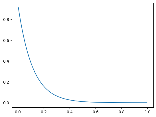
Example: Steady-State Solution of a Plug Flow Reactor
This example demonstrates how to compute a steady-state solution for a plug flow reactor using first-order kinetics. The reactor is modeled as a 1D domain with convection, diffusion, and nonlinear reaction kinetics.
The model is configured to simulate the reaction-diffusion process under steady-state conditions, utilizing the kinetic parameters and boundary conditions defined in the code.
shape = (100,1)
kinetics = Kinetics(shape, 10.0)

bc = ({'a':0, 'b': 1, 'd': 1}, {'a':1, 'b': 0, 'd': 0})
reactor_model = DiffusionConvectionReactionNonLinear(shape, bc = bc, g_kinetics = kinetics.compute_g)
reactor_model.solve()

plt.plot(reactor_model.z_c, reactor_model.c[:,0])
class ParticleModel:
    """
    General 1D (or quasi-1D) reaction-diffusion model for a particle.

    This class models a particle with arbitrary geometry and user-supplied
    nonlinear kinetics. It supports both steady-state and transient solutions,
    and can be used for multi-component systems.

    Parameters
    ----------
    shape : tuple
        Shape of the concentration field (number of grid points, number of components).
    axis : int, optional
        Axis along which the diffusion occurs (default: -2).
    c_0 : float or array, optional
        Initial concentration (default: 0.0).
    R : float, optional
        Particle radius (default: 1.0).
    D : float or array, optional
        Diffusion coefficient(s) (default: 1.0).
    nu : int, optional
        Geometric factor for divergence operator (default: 2).
    dt : float, optional
        Time step size (default: np.inf for steady-state).
    g_kinetics : callable, optional
        Function returning (reaction residual, jacobian) for the nonlinear kinetics.

    Attributes
    ----------
    c : ndarray
        Concentration field.
    c_old : ndarray
        Previous concentration field (for time stepping).
    r_f, r_c : ndarray
        Face and center grid points.
    jac_diff : sparse matrix
        Diffusion Jacobian.
    jac_diff_bc : sparse matrix
        Boundary condition Jacobian.
    r_apparent_mat, r_apparent_bc_mat : ndarray
        Matrices for computing apparent reaction rates.
    numjac : NumJac
        Numerical Jacobian helper for nonlinear kinetics.

    Methods
    -------
    init_field(c_0)
        Initialize the concentration field.
    init_jac()
        Construct the Jacobian matrix and constant terms for the system.
    g(c, c_b)
        Returns (residual, jacobian) for the current time step.
    step_time()
        Updates c_old for time stepping.
    apparent_reaction_rate(c_b, solve=True, compute_jac=False)
        Computes the apparent reaction rate for given boundary concentrations.
    schur_init(c=None)
        Store the current concentration for Schur complement updates.
    schur_post_step(c)
        Update the concentration after a Schur complement step.
    """

    def __init__(self, shape, axis = -2, c_0 = 0.0, R=1.0, D=1.0, nu=2, dt=np.inf, g_kinetics=None):
        """
        Initialize the diffusion-reaction model.

        Parameters
        ----------
        shape : tuple
            Shape of the concentration field (number of grid points, number of components).
        axis : int, optional
            Axis along which the diffusion occurs (default: -2).
        c_0 : float or array, optional
            Initial concentration (default: 0.0).
        R : float, optional
            Particle radius (default: 1.0).
        D : float or array, optional
            Diffusion coefficient(s) (default: 1.0).
        nu : int, optional
            Geometric factor for divergence operator (default: 2).
        dt : float, optional
            Time step size (default: np.inf for steady-state).
        g_kinetics : callable, optional
            Function returning (reaction residual, jacobian) for the nonlinear kinetics.
        """
        # Initialize model parameters
        self.shape = shape  # Shape of the concentration field
        if axis < 0:
            self.axis = len(shape)+ axis  # Axis along which the diffusion occurs
        else:
            self.axis = axis
        self.shape_d = tuple(1 if i == self.axis else s for i, s in enumerate(self.shape))
        self.shape_c_b = tuple(s for i, s in enumerate(shape) if i != self.axis)
        self.nu = nu  # Geometric factor for divergence operator
        self.bc = ({'a': 1, 'b': 0, 'd': 0},  # Left boundary conditions
                   {'a': 0, 'b': 1, 'd': 1})  # Right boundary conditions
        self.D = D  # Diffusion coefficients
        self.R = R  # Particle radius
        self.dt = dt  # Time step size

        # Generate a non-uniform grid for cell-face positions
        dr_large = 0.1 * self.R
        self.r_f = non_uniform_grid(0, self.R, self.shape[self.axis] + 1, dr_large, 0.75)
        self.r_c = 0.5 * (self.r_f[:-1] + self.r_f[1:])

        # Initialize the concentration field and Jacobian matrix
        self.init_field(c_0)
        if (self.dt == np.inf):
            self.c_old = None
        else:
            self.c_old = np.zeros_like(self.c)
        self.init_jac()
        self.g_kinetics = g_kinetics

    def init_field(self, c_0=0.0):
        """
        Initialize the concentration field with a uniform value.

        Parameters
        ----------
        c_0 : float or array, optional
            Initial concentration value(s).
        """
        # Initialize the concentration field with a uniform value (default is 0.0)
        c = np.asarray(c_0)
        shape = (1,) * (len(self.shape) - c.ndim) + c.shape  # Ensure c
        c = c.reshape(shape)  # Reshape c to 2D
        self.c = np.broadcast_to(c, self.shape).copy()  # Broadcast c to the correct shape

    def init_jac(self):
        """
        Construct the Jacobian matrix and constant terms for the system.
        """
        # Construct the Jacobian matrix and constant terms for the system
        grad_mat, _, grad_bc_mat = construct_grad(self.shape, self.r_f, self.r_c, self.bc, axis = self.axis, shapes_d=(None,self.shape_d))
        div_mat = construct_div(self.shape, self.r_f, nu=self.nu, axis = self.axis)

        # Construct diffusion coefficient matrix
        D = np.asarray(self.D)
        if D.ndim == 0:
            D = D[None]
        shape_D = (1,)*(len(self.shape)-D.ndim) + D.shape
        D = D.reshape(shape_D)
        diff_mat = construct_coefficient_matrix(D, shape=self.shape, axis = self.axis)

        # Compute flux terms
        flux_mat = -diff_mat @ grad_mat
        flux_bc_mat = -diff_mat @ grad_bc_mat

        # Compute Jacobian of diffusion term and boundary forcing term
        self.jac_diff = div_mat @ flux_mat
        self.jac_diff_bc = div_mat @ flux_bc_mat
        self.jac_diff_bc_array = self.jac_diff_bc.toarray()

        # Accumulation term for time-dependent problems
        self.jac_accum = construct_coefficient_matrix(1.0 / self.dt, shape=self.shape)

        # Apparent reaction rate terms
        # Use correct indices for the last face (right boundary)
        shape_f_t = (math.prod(self.shape[0:self.axis]), self.shape[self.axis]+1, math.prod(self.shape[self.axis+1:]))
        i_col = (shape_f_t[2]*shape_f_t[1]*np.arange(shape_f_t[0]).reshape((-1, 1)) + shape_f_t[2]*self.shape[self.axis] + np.arange(shape_f_t[2]).reshape((1, -1))).ravel()
        self.r_apparent_mat = ((self.nu + 1) / self.R) * flux_mat[i_col, :]
        self.r_apparent_bc_mat = ((self.nu + 1) / self.R) * flux_bc_mat[i_col, :]

        # Numerical Jacobian for reaction terms
        self.numjac = NumJac(self.shape)

    def g(self, c, c_b):
        """
        Compute the residual vector and Jacobian matrix for the current time step.

        Parameters
        ----------
        c : array
            Current concentration values.
        c_b : array
            Boundary concentration values.

        Returns
        -------
        tuple
            Residual vector and Jacobian matrix.
        """
        # Compute the residual vector and Jacobian matrix for the current time step
        c_b = np.asarray(c_b)
        g = self.jac_diff_bc @ c_b.reshape((-1,1)) + self.jac_diff @ c.reshape((-1, 1))
        jac = self.jac_diff
        if self.c_old is not None:
            g_accum  = self.jac_accum @ (c.reshape((-1, 1)) - self.c_old.reshape((-1, 1)))
            g += g_accum
            jac += self.jac_accum
        if self.g_kinetics is not None:
            g_react, jac_react = self.g_kinetics(c)
            g -= g_react.reshape((-1, 1))
            jac -= jac_react
        return g, jac

    def step_time(self):
        """
        Store the current concentration as the previous value for time stepping.
        """
        self.c_old = self.c.copy()

    def apparent_reaction_rate(self, c_b, solve = False, compute_jac = False):
        """
        Compute the apparent reaction rate based on the current concentration field.

        Parameters
        ----------
        c_b : array
            Boundary concentration values.
        solve : bool, optional
            If True, solve for the steady-state concentration before computing the rate.
        compute_jac : bool, optional
            If True, also compute the Jacobian of the apparent reaction rate.

        Returns
        -------
        array or tuple
            Apparent reaction rates for each component, and optionally the Jacobian.
        """
        if solve and not compute_jac:
            result = newton(lambda c: self.g(c, c_b), self.c, maxfev=10)
            self.c[...] = result.x.reshape(self.shape)

        c_vec = self.c.reshape((-1, 1))
        c_b_vec = np.asarray(c_b).reshape((-1, 1))
        if compute_jac:
            self.c_b_prev = c_b.copy()
            g, jac_ss = self.g(self.c, c_b)
            jac_ss_lu = sla.splu(jac_ss)
            dc = -jac_ss_lu.solve(g)
            c_vec[...] += dc
            r_apparent = self.r_apparent_mat @ c_vec + self.r_apparent_bc_mat @ c_b_vec
            # The Jacobian calculation here is a placeholder; adjust as needed for your application
            self.jac_sf_schur = csc_array(jac_ss_lu.solve(self.jac_diff_bc_array))
            jac = -self.r_apparent_mat @ self.jac_sf_schur + self.r_apparent_bc_mat
            return r_apparent.reshape(self.shape_c_b), jac
        else:
            r_apparent = self.r_apparent_mat @ c_vec + self.r_apparent_bc_mat @ c_b_vec
            return r_apparent.reshape((self.shape_c_b))

    def schur_post_step(self, c_b, g):
        """
        Update the concentration after a Schur complement step.

        Parameters
        ----------
        c : array
            Updated concentration.
        """
        dc_b = c_b - self.c_b_prev
        c_vec = self.c.reshape((-1, 1))
        c_vec[...] -= self.jac_sf_schur @ dc_b
        self.c_b_prev = c_b.copy()
Example: Steady-State Solution of the Particle Model
This example demonstrates how to compute a steady-state solution for a particle model using user-defined kinetics. The particle is modeled as a 1D domain (e.g., spherical or slab geometry) with diffusion and nonlinear reaction kinetics.
The model is configured to simulate the reaction-diffusion process within a particle under steady-state conditions, utilizing the predefined kinetic parameters.
shape_pm = (30,1)
c_b = np.asarray([[1.0]])

kinetics_pm = Kinetics(shape_pm, 1.0)

particle_model = ParticleModel(shape_pm, R=1e-3, D=1e-5, nu=2,  g_kinetics = kinetics_pm.compute_g)
r_app, jac_app = particle_model.apparent_reaction_rate(c_b, compute_jac=True)
plt.plot(particle_model.r_c, particle_model.c[:,0])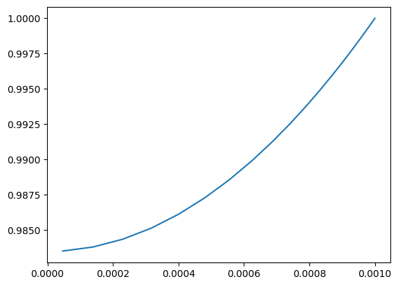
Example: Steady-State Solution of the Particle Model
This example demonstrates how to compute a steady-state solution for a particle model using user-defined kinetics. The particle is modeled as a 1D domain (e.g., spherical or slab geometry) with diffusion and nonlinear reaction kinetics.
The model is configured to simulate the reaction-diffusion process within a particle under steady-state conditions, utilizing the predefined kinetic parameters.
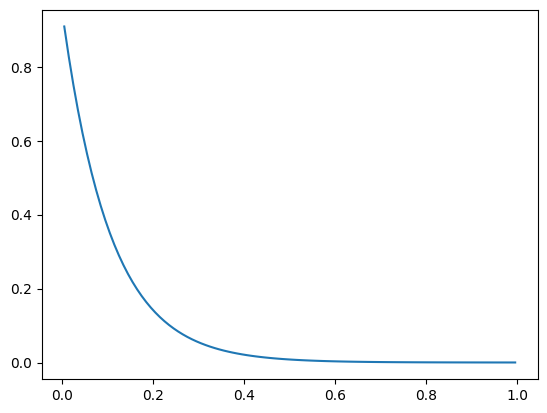
Explicit Coupling and ‘black-box’ Coupling
shape = (100,1)
shape_pm = shape[0:-1] + (30,) + shape[-1:]
kinetics_pm = Kinetics(shape_pm, 10.0)

particle_model = ParticleModel(shape_pm, R=1e-3, D=1e-5, g_kinetics = kinetics_pm.compute_g)
kinetics_app = lambda c_b: particle_model.apparent_reaction_rate(c_b, solve=True)

jac_kinetics_app = csc_array((math.prod(shape), math.prod(shape)))
g_kinetics_app = lambda c: (particle_model.apparent_reaction_rate(c, solve=True), jac_kinetics_app)

#numjac = NumJac(shape)
#g_kinetics_app = lambda c: numjac(kinetics_app, c)

bc = ({'a':0, 'b': 1, 'd': 1}, {'a':1, 'b': 0, 'd': 0})
reactor_model = DiffusionConvectionReactionNonLinear(shape, bc = bc, g_kinetics = g_kinetics_app)
reactor_model.solve()

plt.plot(reactor_model.z_c, reactor_model.c[:,0])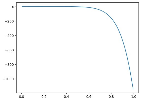
Coupling with Schur complement
shape = (100,1)
shape_pm = shape[0:-1] + (30,) + shape[-1:]
kinetics_pm = Kinetics(shape_pm, 10.0)
particle_model = ParticleModel(shape_pm, R=1e-3, D=1e-5, g_kinetics = kinetics_pm.compute_g)

g_kinetics_app = lambda c_b: particle_model.apparent_reaction_rate(c_b, solve=False, compute_jac=True)
bc = ({'a':0, 'b': 1, 'd': 1}, {'a':1, 'b': 0, 'd': 0})
reactor_model = DiffusionConvectionReactionNonLinear(shape, bc = bc, g_kinetics = g_kinetics_app, callback_newton = particle_model.schur_post_step)
reactor_model.solve()

plt.plot(reactor_model.z_c, reactor_model.c[:,0])