L2: Unsteady Convection-Reaction - Multiphase Reactor Modeling using PyMRM

Convection is the dominant transport mechanism in tubular reactors and column flows. This notebook covers the method of lines (MOL) discretisation of the 1D convection-reaction equation on a cell-centred grid, the stability requirement (Courant condition), and the improvement in accuracy achieved by TVD schemes using the Normalised Variable Diagram (NVD), as implemented in pymrm.

Governing equation¶

\frac{\partial c}{\partial t} + v \frac{\partial c}{\partial z} = R(c)

(1)

Discretised on $N$ cells of width $\Delta z = L/N$ with first-order upwind (FOU):

c_i^{n+1} = c_i^n - Co\left(c_{i+1/2}^n - c_{i-1/2}^n\right), \quad Co = \frac{v\,\Delta t}{\Delta z} \leq 1

(2)

FOU is first-order accurate: it introduces numerical diffusion proportional to $\tfrac{1}{2}v\Delta z(1-Co)$ , which smears sharp fronts.

TVD via the Normalised Variable Diagram (NVD)¶

For a face between cells $C$ (upwind) and $D$ (downwind), define the upstream cell $U$ as the cell one step further upwind of $C$ . The normalised variable is:

\tilde{c}_C = \frac{c_C - c_U}{c_D - c_U}, \quad \tilde{x}_C = \frac{x_C - x_U}{x_D - x_U}, \quad \tilde{x}_f = \frac{x_f - x_U}{x_D - x_U}

(3)

The face concentration is written as:

c_f = c_U + \tilde{c}_f\,(c_D - c_U)

(4)

FOU: $\tilde{c}_f = \tilde{c}_C$ — no correction, highest numerical diffusion
Central differencing: $\tilde{c}_f = \tilde{x}_f$ — may introduce oscillations
TVD (Sweby region): $\tilde{c}_f \in [\tilde{c}_C,\, 1]$ for $\tilde{c}_C \in [0,1]$ — no new extrema, bounded between FOU and linear

The pymrm limiter functions return the correction $\Delta\tilde{c} = \tilde{c}_f - \tilde{c}_C$ , so that $c_f = c_C + \phi(\tilde{c}_C, \tilde{x}_C, \tilde{x}_f) \cdot (c_D - c_U)$ .

PyMRM building blocks¶

Function	Role
`construct_convflux_upwind(shape, x_f, bc, v)`	Sparse matrix for FOU convective fluxes
`interp_cntr_to_stagg_tvd(c, x_f, x_c, bc, v, tvd_limiter)`	Returns `(c_f, dc_f)`: face concentrations and TVD correction
`construct_div(shape, x_f)`	Divergence: maps face fluxes to cell residuals
`minmod`, `vanleer`, `muscl`, `osher`, `clam`	NVD limiter functions $\phi(\tilde{c}_C, \tilde{x}_C, \tilde{x}_f)$

Boundary conditions use the form {'a': a, 'b': b, 'd': d} meaning $a\,(dc/dn) + b\,c_f = d$ :

Dirichlet (specify face value): {'a': 0, 'b': 1, 'd': c_in}
Neumann (specify normal gradient): {'a': 1, 'b': 0, 'd': grad_n}
Zero-gradient outlet: {'a': 1, 'b': 0, 'd': 0}

Example 1 — NVD diagram: comparing limiter functions¶

On a uniform grid $\tilde{x}_C = 0.5$ and $\tilde{x}_f = 0.75$ . The correction $\phi$ as a function of $\tilde{c}_C$ shows each scheme’s behaviour.

import numpy as np
import matplotlib.pyplot as plt
from pymrm import minmod, osher, clam, muscl, vanleer, upwind

x_norm_C = 0.5   # normalised cell-centre position (uniform grid)
x_norm_d = 0.75  # normalised face position (midpoint between C and D)
c_norm = np.linspace(-0.5, 1.5, 400)

limiters = [
    (upwind,  'FOU (upwind)',  'k--'),
    (minmod,  'Min-mod',       'b-'),
    (muscl,   'MUSCL',         'g-'),
    (vanleer, 'van Leer',      'r-'),
    (osher,   'Osher',         'm-'),
]

fig, (ax1, ax2) = plt.subplots(1, 2, figsize=(11, 4))

# Left: NVD diagram — normalised face value vs normalised cell value
for func, name, ls in limiters:
    phi = func(c_norm, x_norm_C, x_norm_d)
    ax1.plot(c_norm, c_norm + phi, ls, label=name)
# Sweby TVD region boundary
ax1.fill_between([0, 1], [0, 1], [0, 1], alpha=0.08, color='green', label='TVD region')
ax1.plot([0, 1], [0, 1], 'g--', lw=0.8)
ax1.plot([0, x_norm_d, 1], [0, x_norm_d, 1], 'gray', lw=0.8, ls=':', label='Central diff.')
ax1.set_xlim(-0.2, 1.2); ax1.set_ylim(-0.2, 1.2)
ax1.set_xlabel(r'$\tilde{c}_C$'); ax1.set_ylabel(r'$\tilde{c}_f$')
ax1.set_title('Normalised Variable Diagram (NVD)')
ax1.legend(fontsize=8)

# Right: the correction phi
for func, name, ls in limiters:
    phi = func(c_norm, x_norm_C, x_norm_d)
    ax2.plot(c_norm, phi, ls, label=name)
ax2.set_xlabel(r'$\tilde{c}_C$')
ax2.set_ylabel(r'$\phi$ (correction $= \tilde{c}_f - \tilde{c}_C$)')
ax2.set_title('TVD correction function $\phi$')
ax2.legend(fontsize=8)

plt.tight_layout(); plt.show()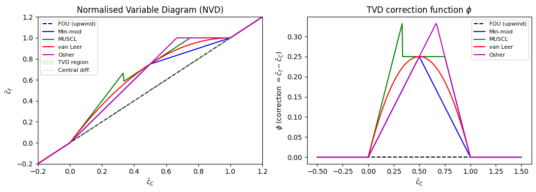

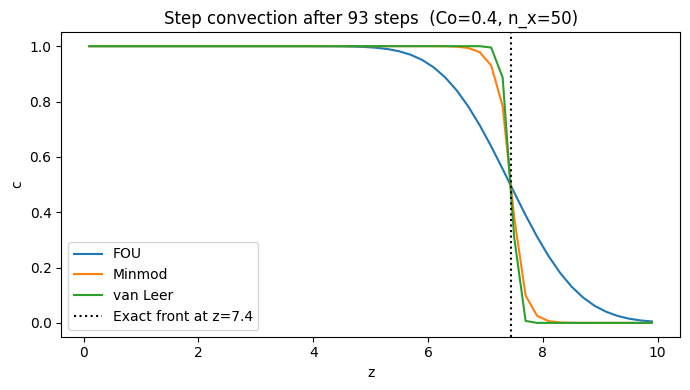
Example 2 — Step convection: FOU vs TVD limiters¶

Explicit Euler time integration with Courant number $Co = 0.4$ . interp_cntr_to_stagg_tvd returns (c_f, dc_f) where dc_f is the TVD correction; the sum c_f + dc_f gives the TVD face concentration directly.

import math
from pymrm import construct_div, interp_cntr_to_stagg_tvd
from pymrm import upwind, minmod, vanleer

length, n_x = 10.0, 50
x_f = np.linspace(0, length, n_x+1)
x_c = 0.5*(x_f[:-1] + x_f[1:])
v = 1.0
Co = 0.4
dt = Co * (x_f[1]-x_f[0]) / v
n_steps = int(0.75 * length / (v*dt))

# Boundary conditions: inlet face value = 1 (a=0,b=1,d=1)
# outlet: zero gradient (a=1,b=0,d=0)
bc = ({'a': 0, 'b': 1, 'd': 1.0}, {'a': 1, 'b': 0, 'd': 0.0})
div_mat = construct_div(n_x, x_f)

fig, ax = plt.subplots(figsize=(7, 4))
for func, name in [(upwind, 'FOU'), (minmod, 'Minmod'), (vanleer, 'van Leer')]:
    c = np.zeros(n_x)
    for _ in range(n_steps):
        c_f, dc_f = interp_cntr_to_stagg_tvd(c, x_f, x_c, bc, v,
                                              tvd_limiter=func, axis=0)
        c += -dt * (div_mat @ (v * c_f)).ravel()
    ax.plot(x_c, c, label=name)

t_final = n_steps * dt
ax.axvline(v*t_final, ls=':', color='k', label=f'Exact front at z={v*t_final:.1f}')
ax.set_xlabel('z'); ax.set_ylabel('c')
ax.set_title(f'Step convection after {n_steps} steps  (Co={Co}, n_x={n_x})')
ax.legend(); plt.tight_layout(); plt.show()

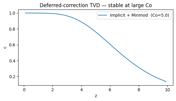
Example 3 — Implicit convection with deferred TVD correction¶

For stiff problems, use implicit (backward-Euler) FOU as the base scheme and apply the TVD correction explicitly as a deferred correction: solve the linear FOU system and then correct the right-hand side with $\mathbf{D}\cdot(v\,\delta c_f)$ .

import scipy.sparse as sp, scipy.sparse.linalg as sla
from pymrm import construct_convflux_upwind, construct_div
from pymrm import minmod

L2, n_x = 10.0, 50
x_f2 = np.linspace(0, L2, n_x+1)
x_c2 = 0.5*(x_f2[:-1] + x_f2[1:])
v2, Co2 = 1.0, 5.0   # large Courant number — explicit would be unstable!
dt2 = Co2 * (x_f2[1]-x_f2[0]) / v2
n2 = int(0.75 * L2 / (v2*dt2))
bc2 = ({'a': 0, 'b': 1, 'd': 1.0}, {'a': 1, 'b': 0, 'd': 0.0})

conv_mat, conv_bc = construct_convflux_upwind(n_x, x_f2, x_c2, bc2, v2)
div_mat = construct_div(n_x, x_f2)
# Implicit FOU Jacobian (constant → factor once)
jac_const = sp.eye(n_x, format='csc') / dt2 + div_mat @ conv_mat
jac_lu = sla.splu(jac_const)

c2 = np.zeros(n_x)
for _ in range(n2):
    c_old = c2.copy()
    for _ in range(2):  # 1-2 inner iterations sufficient
        _, dc_f2 = interp_cntr_to_stagg_tvd(c2, x_f2, x_c2, bc2, v2,
                                             tvd_limiter=minmod, axis=0)
        rhs = c_old / dt2 - (div_mat @ (conv_bc + v2*dc_f2.reshape(-1,1))).ravel()
        c2 = jac_lu.solve(rhs)

plt.figure(figsize=(6, 3.5))
plt.plot(x_c2, c2, label=f'Implicit + Minmod  (Co={Co2})')
plt.xlabel('z'); plt.ylabel('c')
plt.title('Deferred-correction TVD — stable at large Co')
plt.legend(); plt.tight_layout(); plt.show()

Summary¶

Scheme	$\tilde{c}_f$ (NVD)	Order	Stable?
FOU (upwind)	$\tilde{c}_C$	1	Yes, $Co \leq 1$
Central	$\tilde{x}_f$	2	No (oscillations)
Minmod	$\tilde{c}_C + \phi_{\text{MM}}$	2 in smooth regions	Yes (TVD)
van Leer	$\tilde{c}_C + \phi_{\text{VL}}$	2	Yes (TVD)

NVD normalises concentration relative to upstream/downstream pair: scheme properties become independent of grid size
Deferred correction: solve implicit FOU system, correct RHS with TVD term — combines A-stability of implicit with accuracy of TVD
Numerical diffusion of FOU ∝ $\tfrac{1}{2}v\Delta z(1-Co)$ — reduces with grid refinement or with TVD
pymrm: interp_cntr_to_stagg_tvd returns (c_f, dc_f); add Div @ (v*dc_f) to the explicit RHS correction