L1: ODE Solving for Reactor Modeling - Multiphase Reactor Modeling using PyMRM

Reactor models frequently reduce to systems of ordinary differential equations (ODEs). For batch reactors and plug-flow reactors all spatial gradients vanish or are replaced by the residence time coordinate. This notebook demonstrates how to formulate and solve such models using explicit and implicit methods in Python.

Governing equations¶

A multicomponent reacting system with $n_c$ species and $n_r$ reactions:

\frac{d\mathbf{c}}{dt} = \boldsymbol{\nu}^T \mathbf{r}(\mathbf{c}, T)

(1)

\frac{dT}{dt} = -\frac{\boldsymbol{\Delta H}^T \mathbf{r}(\mathbf{c}, T)}{\rho c_p}

(2)

where $\boldsymbol{\nu}$ is the $(n_r \times n_c)$ stoichiometric matrix, $\mathbf{r}$ the vector of reaction rates, and $\Delta H_j$ the heat of reaction $j$ .

The stoichiometric matrix encodes mass conservation; each column sums to zero for closed systems.

Forward (explicit) Euler — first-order, conditionally stable:

\mathbf{c}^{n+1} = \mathbf{c}^n + \Delta t\, \mathbf{f}(\mathbf{c}^n)

(3)

Backward (implicit) Euler — first-order, unconditionally stable (A-stable):

\mathbf{c}^{n+1} = \mathbf{c}^n + \Delta t\, \mathbf{f}(\mathbf{c}^{n+1})

(4)

The implicit step requires solving a nonlinear system at each time level.

PyMRM building blocks¶

Function / module	Role
`scipy.integrate.solve_ivp`	Adaptive Runge–Kutta integration (BDF for stiff systems)
`pymrm.NumJac`	Finite-difference Jacobian approximation
`pymrm.newton`	Newton–Raphson solver for nonlinear systems
`numpy` stoichiometric matrix	Encodes reaction network; `nu @ r(c)` gives rate vector

Example 1 — Consecutive reactions A → B → C in a batch reactor¶

Parameters: $k_1 = 1\,\text{s}^{-1}$ , $k_2 = 0.5\,\text{s}^{-1}$ , $c_{A,0} = 1\,\text{mol/m}^3$ .

import numpy as np
import matplotlib.pyplot as plt
from scipy.integrate import solve_ivp

k1, k2 = 1.0, 0.5          # rate constants [1/s]
nu = np.array([[-1, 0],     # stoichiometric matrix (nc x nr)
               [ 1,-1],
               [ 0, 1]])

def rates(c): return np.array([k1*c[0], k2*c[1]])
def rhs(t, c): return nu @ rates(c)

c0 = np.array([1.0, 0.0, 0.0])
sol = solve_ivp(rhs, [0, 8], c0, dense_output=True, rtol=1e-8)

t = np.linspace(0, 8, 300)
C = sol.sol(t)
plt.figure(figsize=(6, 3.5))
for i, label in enumerate(['A', 'B', 'C']):
    plt.plot(t, C[i], label=label)
plt.xlabel('Time (s)'); plt.ylabel('Concentration (mol/m³)')
plt.title('Batch reactor: A → B → C')
plt.legend(); plt.tight_layout(); plt.show()
print(f'Maximum B concentration: {C[1].max():.4f} at t = {t[C[1].argmax()]:.2f} s')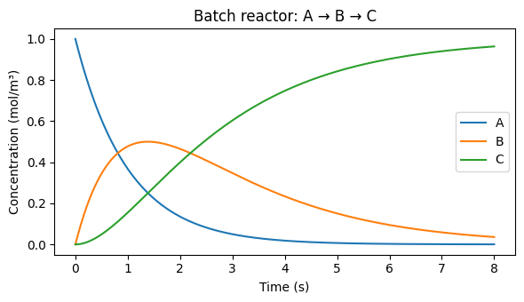

Maximum B concentration: 0.5000 at t = 1.39 s

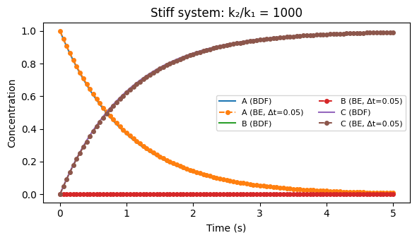
Example 2 — Stiff system: explicit vs implicit Euler¶

A stiff system has widely separated time scales. Here $k_1 = 1$ and $k_2 = 1000\,\text{s}^{-1}$ to create stiffness. The explicit Euler method requires $\Delta t < 1/k_2 = 10^{-3}\,\text{s}$ for stability, while backward Euler remains stable with much larger time steps.

from scipy import sparse
from pymrm import NumJac, newton

k1_s, k2_s = 1.0, 1000.0
nu_s = np.array([[-1, 0], [1, -1], [0, 1]])

def rhs_s(c): return nu_s @ np.array([k1_s*c[0], k2_s*c[1]])

# Backward Euler with Newton solve
dt = 0.05   # large step — stable for implicit, unstable for explicit
t_end = 5.0
t_be, c_be = [0.0], [np.array([1.0, 0.0, 0.0])]
c = c_be[0].copy()
t = 0.0
numjac = NumJac(c.shape)
while t < t_end - 1e-10:
    c_old = c.copy()
    def residual(c_new):
        g = c_new - c_old - dt * rhs_s(c_new)
        _, jac_rhs = numjac(rhs_s, c_new)
        jac = sparse.eye(len(c_new), format='csc') - dt * jac_rhs
        return g.reshape(-1, 1), jac
    result = newton(residual, c.copy())
    c = result.x.ravel()
    t += dt; t_be.append(t); c_be.append(c.copy())

t_be = np.array(t_be)
c_be = np.array(c_be)

# Reference: solve_ivp (BDF)
sol_ref = solve_ivp(lambda t, c: rhs_s(c), [0, t_end],
                    [1.0, 0.0, 0.0], method='BDF', dense_output=True)
t_ref = np.linspace(0, t_end, 500)
C_ref = sol_ref.sol(t_ref)

fig, ax = plt.subplots(figsize=(6, 3.5))
for i, lab in enumerate(['A', 'B', 'C']):
    ax.plot(t_ref, C_ref[i], lw=1.5, label=f'{lab} (BDF)')
    ax.plot(t_be, c_be[:, i], 'o--', ms=4, label=f'{lab} (BE, Δt={dt})')
ax.set_xlabel('Time (s)'); ax.set_ylabel('Concentration')
ax.set_title(f'Stiff system: k₂/k₁ = {k2_s/k1_s:.0f}')
ax.legend(ncol=2, fontsize=8); plt.tight_layout(); plt.show()

Summary¶

Method	Order	Stability	Recommended for
Forward Euler	1	Conditional ( $\Delta t < 2/\lambda_{\max}$ )	Non-stiff, simple
Backward Euler	1	Unconditional (A-stable)	Stiff systems, moderate accuracy
`solve_ivp` RK45	4/5	Conditional (adaptive)	Non-stiff, high accuracy
`solve_ivp` BDF	1–5	Stiff-safe (adaptive)	Stiff chemical kinetics

Key insight: The stoichiometric matrix $\boldsymbol{\nu}$ is the central data structure. Defining it once lets you swap reaction networks without rewriting the integrator.