Rejection-free Monte Carlo: the Lennard-Jones fluid

This notebook reproduces the Lennard-Jones example of E.A.J.F. Peters and G. de With, Rejection-free Monte Carlo sampling for general potentials, Phys. Rev. E 85, 026703 (2012), with spheropack.rejection_free.

In the rejection-free method all particles move along straight lines. For every pair, the increase of the pair potential along the path is accumulated (decreases are free), and the pair reflects like an elastic collision when the accumulated increase reaches \(-kT\ln u\) with \(u\) uniform in \((0, 1]\). No move is ever rejected, and positions sampled at equidistant times follow the canonical distribution \(\exp(-U/kT)\).

# Install spheropack when it is not available (for example on Google Colab).
import importlib.util

if importlib.util.find_spec("spheropack") is None:
    %pip install -q spheropack

import time
from pathlib import Path

import matplotlib.pyplot as plt
import numpy as np

import spheropack as sp
from spheropack import rejection_free as rf

The potential

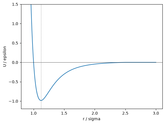
The truncated and shifted Lennard-Jones potential, \(U(r) = 4\epsilon[(\sigma/r)^{12} - (\sigma/r)^6] - U_\mathrm{LJ}(r_c)\) for \(r < r_c = 2.5\sigma\). Approaching particles accumulate potential increase only inside the minimum at \(r = 2^{1/6}\sigma\); separating particles accumulate it between the minimum and the cutoff.

lj = rf.LennardJones(epsilon=1.0, sigma=1.0, cutoff=2.5)
r = np.linspace(0.9, 3.0, 400)
plt.plot(r, lj(r))
plt.axhline(0, color="k", lw=0.5)
plt.axvline(2 ** (1 / 6), color="k", lw=0.5, ls=":")
plt.ylim(-1.2, 1.5)
plt.xlabel("r / sigma"); plt.ylabel("U / epsilon");

The state point of the paper

1000 particles at number density \(\rho = 0.317\) and temperature \(T = 1.085\) (Lennard-Jones units), close to the critical point. To avoid huge initial energies the particles start from a random packing of spheres of diameter \(0.9\sigma\), generated with spheropack.pack.

n, rho, T = 1000, 0.317, 1.085
L = (n / rho) ** (1 / 3)
start = sp.pack(n=n, radii=0.45, container=sp.PeriodicBox(L), seed=1)
system = rf.System(start.positions, box=start.container, potential=lj, kT=T, seed=1)
system

System(n=1000, dim=3, density=0.317, potential=LennardJones(rc=2.5), kT=1.085, method='collisions', time=0, n_reflections=0)

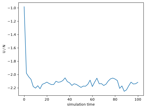
Equilibration: the potential energy per particle settles within a few tens of time units (time is the contour length of the moves; the move velocities are Gaussian with unit variance per component).

times, energies = [0.0], [system.potential_energy() / n]
t0 = time.perf_counter()
for _ in range(50):
    system.run(2.0)
    times.append(system.time)
    energies.append(system.potential_energy() / n)
print(f"{system.n_reflections} reflections in {time.perf_counter() - t0:.1f} s")
plt.plot(times, energies)
plt.xlabel("simulation time"); plt.ylabel("U / N");

583643 reflections in 7.9 s

Radial distribution function

Sampling every 2 time units; rf.radial_distribution advances the system and averages \(g(r)\) over the samples. The reference data of the paper are three long Metropolis runs and the paper’s own rejection-free run.

t0 = time.perf_counter()
g = rf.radial_distribution(system, n_samples=300, interval=2.0, r_max=5.0, bins=1000)
print(f"sampling took {time.perf_counter() - t0:.0f} s, {system.n_reflections} reflections in total")

def load_reference(name):
    local = Path("../data") / name
    if local.exists():
        return np.loadtxt(local)
    url = f"https://raw.githubusercontent.com/computational-chemical-engineering/spheropack/main/docs/data/{name}"
    return np.loadtxt(url)

ref = load_reference("GofR_LJ_all.dat")
metropolis = ref[:, [1, 3, 5]].mean(axis=1)

fig, axes = plt.subplots(1, 2, figsize=(12, 4))
axes[0].plot(ref[:, 0], metropolis, "k-", lw=2, label="Metropolis (paper)")
axes[0].plot(ref[:, 6], ref[:, 7], lw=1, label="rejection-free (paper)")
axes[0].plot(g.r, g.g, lw=1, label="spheropack")
axes[0].set_xlim(0.8, 5); axes[0].set_xlabel("r / sigma"); axes[0].set_ylabel("g(r)"); axes[0].legend()

coarse = lambda a: a.reshape(100, 10).mean(axis=1)
axes[1].plot(coarse(g.r), coarse(g.g) - coarse(metropolis), "o-", ms=3)
axes[1].axhline(0, color="k", lw=0.5)
axes[1].set_xlim(0.8, 5); axes[1].set_xlabel("r / sigma"); axes[1].set_ylabel("g - g(Metropolis), bins of 0.05")
print(f"mean |difference| on bins of 0.05: {np.abs(coarse(g.g) - coarse(metropolis)).mean():.4f}")

sampling took 50 s, 4065407 reflections in total
mean |difference| on bins of 0.05: 0.0021

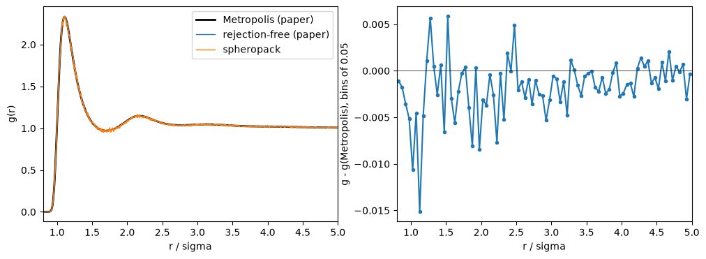
The rejection-free sampling reproduces the Metropolis result within the statistical noise. The paper’s rejection-free run (time 339240) is far longer than this example; the noise of the difference shrinks with the square root of the sampling time.

The DPD liquid of the paper

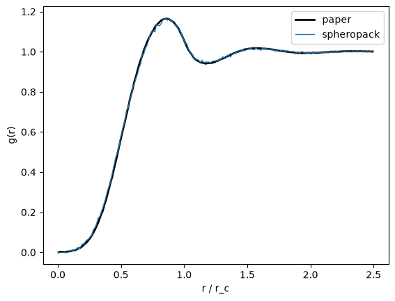
The second example of the paper: DPD particles (soft repulsion \(\frac{a}{2}(1 - r/r_c)^2\)) at the conventional density \(\rho = 3\) with \(a = 25\,kT\), where the particles overlap strongly.

Event chains

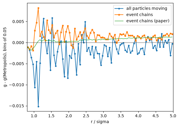
The paper’s second implementation moves one particle at a time: at a reflection the moving particle stops and its partner continues in the same direction. With irreversible chains (directions \(+x, +y, +z\) in turn, the default) this is considerably faster. Time is again the mean displacement per particle.

chain = rf.System(start.positions, box=start.container, potential=lj, kT=T, seed=2, method="event_chain")
chain.run(100.0)
t0 = time.perf_counter()
g_chain = rf.radial_distribution(chain, n_samples=1500, interval=1.0, r_max=5.0, bins=1000)
print(f"event chains: 1500 samples in {time.perf_counter() - t0:.0f} s")

plt.plot(coarse(g.r), coarse(g.g) - coarse(metropolis), "o-", ms=3, label="all particles moving")
plt.plot(coarse(g_chain.r), coarse(g_chain.g) - coarse(metropolis), "s-", ms=3, label="event chains")
plt.plot(coarse(ref[:, 8]), coarse(ref[:, 9]) - coarse(metropolis), lw=1, label="event chains (paper)")
plt.axhline(0, color="k", lw=0.5)
plt.xlim(0.8, 5); plt.xlabel("r / sigma"); plt.ylabel("g - g(Metropolis), bins of 0.05"); plt.legend();

event chains: 1500 samples in 51 s

dpd = rf.System(n=375, box=sp.PeriodicBox(5.0), potential=rf.DPD(a=25.0), kT=1.0, seed=2)
dpd.run(20.0)
g_dpd = rf.radial_distribution(dpd, n_samples=400, interval=0.5, r_max=2.5, bins=200)
ref_dpd = load_reference("GofR_DPD_110925.dat")
plt.plot(ref_dpd[:, 0], ref_dpd[:, 1], "k-", lw=2, label="paper")
plt.plot(g_dpd.r, g_dpd.g, lw=1, label="spheropack")
plt.xlabel("r / r_c"); plt.ylabel("g(r)"); plt.legend();

Notes

• The move velocities are not physical momenta: their magnitude only sets the time scale of the moves, and they are conserved by the reflections. system.redraw_velocities() draws new ones; the paper found that this is not needed for ergodicity.

• Any pair potential with at most one minimum fits the method: rf.LennardJones, rf.WCA, rf.DPD, rf.SoftSpheres (harmonic, Hertzian) and rf.HardSpheres, where every approach to contact reflects.