# Bootstrap: the pymrm this page was checked with, and the gallery files it was
# published with. Works in a checkout, in CI and on a fresh Colab VM.
GALLERY_REF = "gallery-2026.11.10.3"  # replaced by the release tag at publication
PYMRM = ">=3.4.0,<4"  # equals meta.yaml pymrm_min_version, up to the next major
PAGE = "J3.5-single-particle-model"  # equals the page directory

import os, sys, urllib.request
from pathlib import Path
_shared = next((p / "shared" for p in (Path.cwd(), *Path.cwd().parents)
                if (p / "shared" / "gallery_bootstrap.py").is_file()), None)
if _shared is None:
    _shared = (Path(os.environ.get("XDG_CACHE_HOME") or Path.home() / ".cache")
               / "pymrm-gallery" / GALLERY_REF)
    _shared.mkdir(parents=True, exist_ok=True)
    urllib.request.urlretrieve(
        "https://raw.githubusercontent.com/computational-chemical-engineering/"
        f"pymrm-gallery/{GALLERY_REF}/shared/gallery_bootstrap.py",
        _shared / "gallery_bootstrap.py")
sys.path.insert(0, str(_shared))
sys.modules.pop("gallery_bootstrap", None)
from gallery_bootstrap import setup
setup(PAGE, PYMRM, GALLERY_REF); # the semicolon stops the cell echoing the pathHow much battery model do you actually need?
sec:J
struct:S8
struct:S10
struct:S3
tier:T1
data:tier6
phase:liquid-solid
Marquis et al.’s asymptotic reduction of the Doyle–Fuller–Newman model, the SPM and the SPMe, applied to the gallery’s own 1993 cell, with the error scaling the asymptotics promise measured against the full model.
How much battery model do you actually need?
Catalog ID: J3.5 · Structures: S8 (coupled multi-phase transport with electroneutrality), S10 (porous electrode with a distributed interfacial reaction), reduced towards S3 · Tier: T1
The full pseudo-two-dimensional battery model (J3.4) is too expensive for the places most battery models actually run: battery management systems, pack simulations, parameter estimation loops. The industry answer is the single particle model (SPM) and its electrolyte-corrected extension (SPMe). This page builds both, not as ad-hoc simplifications but as the leading- and first-order terms of a systematic asymptotic expansion, and then measures whether the errors shrink at the rate the asymptotics promise.
# Imports. The page's model.py is put on sys.path by setup(); its first part is
# J3.4's model.py, copied unchanged.
import numpy as np
import matplotlib.pyplot as plt
from IPython.display import Markdown, display
from pymrm import describe_bc
from pymrm.checks import find_roots, observed_orders
from gallery_utils import load_data, load_meta, cite_data, Claims, load_claims
from model import (Cell, SPMe, F_CONST, bv_eta, bv_invert, c_e, c_r, crossing, dfn_at, eta_anode,
                   i_eq17, kappa_from_delta, kappa_from_nu, kappa_hat, ocp, pre0, rtf, s_c,
                   s_s, sigma_bar, t_full, u_of_t, v_spm)

plt.rcParams.update({"figure.dpi": 110, "axes.grid": True, "grid.alpha": 0.3})
claims = Claims(PAGE.split("-")[0])
PAGE_J34 = "J3.4-doyle-fuller-newman"
EPS = np.finfo(float).eps
BREAK = []   # (injected defect, claim, clean value, broken value, caught)


def brk(row, metric, broken):
    """One injected defect: ``broken`` is what claim ``metric`` becomes with it."""
    caught = claims.breaks(row, metric, broken)
    BREAK.append((row, metric, claims[metric], broken, caught))


def run_row(row, d):
    """Every registered claim in ``d`` gets the row."""
    for k, v in d.items():
        if not k.startswith("_") and k in claims.metrics:
            brk(row, k, v)


def rms(d):
    return float(np.sqrt(np.mean(np.square(d))))


def orders_with_ratio(vals, ratio):
    """Orders of consecutive triples read with an assumed refinement ratio (break rows only)."""
    v = [np.asarray(x, float) for x in vals]
    d = [np.max(np.abs(v[k] - v[k + 1])) for k in range(len(v) - 1)]
    return [float(np.log(d[k] / d[k + 1]) / np.log(ratio)) for k in range(len(d) - 1)]
Background
The Doyle–Fuller–Newman (DFN) model couples salt transport, two potentials and particle-scale diffusion through a nonlinear reaction distributed over the electrode. Most of the time, most of that machinery is idle: at low current the electrolyte is nearly uniform, the potentials are nearly flat, and every particle in the electrode does the same thing. The SPM is what is left: one representative particle per electrode and an algebraic voltage expression.
For twenty years the literature extended the SPM with electrolyte corrections by ad-hoc argument, each version keeping a different subset of terms. Marquis, Sulzer, Timms, Please and Chapman (2019) replaced the guesswork with an asymptotic derivation: expand the DFN model in \(\mathcal{C}_e\), the ratio of the electrolyte transport timescale to the discharge timescale, in the distinguished limit where the ohmic drops are comparably small. At leading order the SPM falls out; at first order, one linear PDE for the electrolyte correction plus an algebraic voltage correction, the SPMe. The derivation buys two things no ad-hoc model has: an a-priori applicability test (their Table VI), and a predicted error scaling: the SPM voltage error is \(O(\mathcal{C}_e)\) and the SPMe error \(O(\mathcal{C}_e^2)\).
This page applies their derivation to the cell the DFN model was born on: the Li | separator | TiS\(_2\) half-cell of Doyle, Fuller & Newman (1993), exactly as implemented on J3.4. The full model, its parameter set and its reductions then live in one place, and the reduced models are tested against a full solution whose own fidelity the gallery has already established.
Nothing on this page touches a measurement. The J3.4 reference is a reproduction of a published simulation (its Figure 2 has no experimental points), and every comparison here is reduced model against full model. This page is tier 6 twice over, and says so.
The published model
Marquis et al. start from the DFN model (their Eqs. 1), nondimensionalise (their Tables II and III), and take the limit \(\mathcal{C}_e \to 0\) with
\[ \mathcal{C}_e = \frac{\tau_e}{\tau_d} = \frac{I\,L^2}{D_e\,F\,c_{\rm cap}\,\delta_{\rm cap}} \ll 1 , \qquad \bar\sigma_k = \frac{RT/F}{I L/\sigma_k} \gg 1 , \qquad \hat\kappa_e = \frac{RT/F}{I L/\kappa_e} \gg 1 , \]
in the distinguished limit \(\bar\sigma_k \mathcal{C}_e,\ \hat\kappa_e \mathcal{C}_e = O(1)\). Here \(\tau_e\) is the electrolyte diffusion time over the whole cell of thickness \(L\) and \(\tau_d\) the discharge time set by the electrode capacity.
Leading order, the SPM (their Eqs. 20). The electrolyte concentration is uniform, both potentials are flat, and the transfer current is uniform in each electrode, so every particle behaves identically. What remains is diffusion in one representative particle per electrode with a known surface flux, and a voltage that is open-circuit potential plus reaction overpotentials.
First order, the SPMe (their Eqs. 40, dimensional summary in their Eqs. 48). The corrections are: one linear diffusion PDE for the electrolyte perturbation \(c^1_e(x,t)\), forced by the known leading-order migration flux; and four algebraic voltage terms: a concentration overpotential \(2(RT/F)(1-t^0_+)\,\Delta \bar c_e/c_{e,\rm typ}\), an electrolyte ohmic drop \(-I\,(\frac{L_n}{3\kappa_n^{\rm eff}}+\frac{L_s}{\kappa_s^{\rm eff}} +\frac{L_p}{3\kappa_p^{\rm eff}})\), matrix ohmic drops, and a correction to the exchange-current densities averaged over each electrode. Their key step is that every term is electrode-averaged, not pointwise: averaging the exact voltage identity (their Eq. 10) over all current paths is what makes the expression correct to \(O(\mathcal{C}_e^2)\), and it is the step the ad-hoc models skip. Their Figure 7 shows the canonical SPMe outperforming every ad-hoc variant at every C-rate.
The paper also states the price (their Eq. 49): the model error at a given time is \(O(\mathcal{C}_e^2)\), with a prefactor that grows where the OCV is strongly curved. And it gives the conditions to check before trusting the reduction (their Table VI), evaluated below for the Doyle cell.
The same reduction for the 1993 half-cell
The J3.4 cell is Li foil | separator (\(\epsilon=1\)) | porous TiS\(_2\) cathode, with the lithium foil a plane, so only the cathode needs the electrode-averaging step; the anode terms are genuinely pointwise. Following the paper’s path argument (their Eq. 6) from foil to collector and averaging uniformly over the reaction point \(x_p\) in the cathode:
\[ V \;=\; \underbrace{\overline{\Phi_1(x_p)-\Phi_2(x_p)}}_{\text{cathode kinetics + OCP}} \;+\; \underbrace{\overline{\Phi_2(x_p)-\Phi_2(0)}}_{\text{electrolyte}} \;-\; \underbrace{\eta_{s1}}_{\text{foil kinetics}} \;-\; \underbrace{\frac{I\delta_c}{2\sigma}}_{\text{matrix}} . \]
Leading order (SPM). Doyle’s group \(S_c\) (their Eq. 26), the particle diffusion time over the discharge time, is far below one for this cell (it is evaluated below, and on J3.4), so diffusion inside the particle is negligible too and the entire solid state is one number: the utilisation \(u(t) = u_0 + I t/(F(1-\epsilon)c_T\delta_c)\), exact coulomb counting, which charge conservation makes exact for the full model as well (checked below). The uniform transfer current is \(i = -I/(a\delta_c)\), and Eq. 17 of Doyle et al. inverts in closed form when \(\alpha_a=\alpha_c=\alpha\): with \(B = i/[Fk_2(c_{\max}-c)^{\alpha}c^{\alpha}]\),
\[ c_s z^2 - B z - (c_T-c_s) = 0, \qquad \Phi_1-\Phi_2 = U' (c_s) + \frac{RT}{\alpha F}\ln z , \]
taking the positive root \(z\). At \(I\to0\) this reduces exactly to the Eq. 16 open-circuit potential. The SPM voltage is therefore purely algebraic:
\[ V^0(u, I) = U'(uc_T) + \frac{RT}{\alpha F}\ln z\big|_{c=c_0} - \eta_{s1}(I, c_0) - \frac{I\delta_c}{2\sigma}. \]
First order (SPMe). The electrolyte perturbation \(\tilde c = c - c_0\) satisfies
\[ \epsilon(x)\frac{\partial \tilde c}{\partial t} = \frac{\partial}{\partial x}\Big(\epsilon^{1/2} D \frac{\partial \tilde c}{\partial x}\Big) + s(x), \qquad s = \begin{cases} 0 & \text{separator} \\ -\dfrac{(1-t^0_+)I}{F\delta_c} & \text{cathode}, \end{cases} \]
with zero total salt flux at both ends, and the voltage becomes
\[ V^1 = U'(uc_T) + \frac{RT}{\alpha F}\ln \bar z \;-\; I\Big(\frac{\delta_s}{\kappa} + \frac{\delta_c}{3\kappa\epsilon^{3/2}}\Big) \;+\; \frac{2RT}{F}(1-t^0_+)\frac{\langle\tilde c\rangle_c - \tilde c(0)}{c_0} \;-\; \eta_{s1}\big(I, c(0)\big) - \frac{I\delta_c}{2\sigma}, \]
where \(\bar z\) uses the exchange-current prefactor averaged over the cathode (their Eqs. 48n and 48o), \(\langle\tilde c\rangle_c\) is the plain average over the cathode, and \(\tilde c(0)\) the value at the foil. The \(\delta_c/3\) in the ohmic term is the electrode-averaging of the linearly decaying current, the half-cell twin of their Eq. 48p.
Because the discharge here is galvanostatic and the forcing constant, the PDE also has a closed-form quasi-steady solution, piecewise quadratic in \(x\), which is Marquis et al.’s steady-state variant SPMe(S) and doubles as an exact solution to test the pymrm operators against.
Parameters and assumptions
Every physical parameter comes from the J3.4 page, loaded from its reviewed dataset: the Doyle (1993) Tables I and II values read off 600 dpi renders, with the Eq. 16 and 20 open-circuit constants that J3.4 checked against the paper’s own plotted curve. Nothing is re-derived here, and nothing is fitted.
Three inherited choices matter, all settled on J3.4 and kept identical in the full model and the reductions, because a reduction must be compared against the model it was derived from:
- The conductivity \(\kappa\) is J3.4’s reconstruction: a constant recovered from the paper’s own dimensionless group \(\delta\) (Eq. 28). The Eq. 29 route gives a different value; both are computed below.
- The salt-flux Bruggeman exponent is \(D\epsilon^{1/2}\) and the conductivity’s is \(\kappa\epsilon^{3/2}\), as J3.4 established from the paper’s own Figure 2.
- The factor 2 in the concentration term of the current equation (thermodynamics of a 1:1 salt) is kept, as on J3.4.
Reduction-specific assumptions, both first-order consistent: the transference number is evaluated at \(c_0\) in the SPMe (the DFN lets it vary with \(c\)), and the Butler–Volmer concentration prefactors enter through their cathode average.
What a shared parameter error is invisible to. Using one parameter set for both models is what makes the measured error the reduction’s error, and it is exactly what stops this page from testing the parameters. \(U_{\rm ocp}\), \(k_2\), \(\sigma\), \(i_{0,1}\) and above all \(\kappa\) enter the full model and the reductions identically, so an error in any of them largely cancels in every comparison here. \(\kappa\) is the one that matters, because it is the reconstructed input. The Validation section measures how much of the gap between its two routes survives into the comparison.
One honesty note before any number: because this cell’s \(\kappa\) and \(D\) are constants, the SPMe’s ohmic and diffusive corrections have exactly the right functional form, so the SPMe will look better here than it can on a cell with concentration-dependent properties (as in Marquis et al.’s own comparison, where \(\kappa_e(c_e)\) varies). The error that remains is the asymptotic truncation error, which is what this page wants to measure, but the absolute mV numbers should not be read across to other chemistries.
The data
Four datasets, with sharply different roles.
J3.4’s doyle-fuller-newman-1993-parameters.csv (loaded from that page) is the only source of physical inputs. It is the maintainer-reviewed Doyle 1993 parameter set; its provenance and its one reconstructed input are documented on the J3.4 page. J3.4’s doyle-fuller-newman-1993-stated-results.csv supplies the two printed groups \(\delta\) and \(\nu\) the conductivity is recovered from, Doyle’s printed \(S_s\) and \(S_c\), and the utilisation at which the \(I=20\) curve collapses. What J3.4 established about these rows and uses here: \(S_s\) and \(S_c\) recompute to the printed values; the \(\delta\) (Eq. 28) and \(\nu\) (Eq. 29) routes to \(\kappa\) disagree; the Eq. 28 route is the one J3.4 runs. Nothing on J3.4 flags a row this page uses as wrong.
marquis-2019-table1-parameters.csv is Marquis et al.’s Table I, their graphite | LiPF\(_6\) | LCO parameter set. It runs no model here, because the paper prints the numbers but not the functional forms \(U_n(c)\), \(U_p(c)\), \(D_e(c_e)\), \(\kappa_e(c_e)\) that go with them; for those it cites Newman’s DUALFOIL and Moura’s fastDFN codes. That puts a full re-run of their cell out of reach of the printed paper, which is why the validation below reproduces their derived tables and their error scaling rather than their Table IV. This table feeds exactly one thing: the arithmetic reproduction of their Tables II and III.
marquis-2019-stated-results.csv is every derived number the paper prints: the six timescales of Table II, the dimensionless parameters of Table III, the RMS voltage errors of Table IV (their cell, context only), and one in-text value of \(\mathcal{C}_e\) that turns out to disagree with their own Table III.
par = load_data("doyle-fuller-newman-1993-parameters.csv", page=PAGE_J34)
dstat = load_data("doyle-fuller-newman-1993-stated-results.csv", page=PAGE_J34)
mq1 = load_data("marquis-2019-table1-parameters.csv", page=PAGE)
mqs = load_data("marquis-2019-stated-results.csv", page=PAGE)
mq1_meta = load_meta("marquis-2019-table1-parameters.csv", page=PAGE)
mqs_txt = load_data("marquis-2019-stated-results.csv", page=PAGE, dtype=str)   # printed digits

P = {r.symbol: float(r.value) for r in par.itertuples()}
tab2 = {(r.quantity, r.conditions): float(r.value) for r in dstat.itertuples()}
TAB2 = "I = 10 A/m2 with the Table II parameters"
INIT = "initial concentrations"
DELTA, NU = tab2[("delta", INIT)], tab2[("nu", INIT)]
BRUG = P["epsilon"] ** 1.5
KAPPA = kappa_from_delta(DELTA, P) / BRUG          # bulk; kappa_eff = KAPPA eps^1.5 (J3.4)
KAPPA_29 = kappa_from_nu(NU, P) / BRUG             # the Eq. 29 route, for the sensitivity
RTF = rtf(P)
M = {r.symbol: float(r.value) for r in mq1.itertuples()}
STATED = {r.quantity: float(r.value) for r in mqs.itertuples()}


def last_digit(text):
    """Place value of the last printed digit of a number written as ``text``."""
    mant, _, exp = text.strip().lower().partition("e")
    return 10.0 ** (int(exp or 0) - (len(mant.split(".")[1]) if "." in mant else 0))


UNIT = {r.quantity: last_digit(r.value) for r in mqs_txt.itertuples()}
print(f"J3.4 parameter set: {len(par)} values (see the J3.4 page for provenance)")
print(f"delta = {DELTA:g}, nu = {NU:g} (J3.4 stated results): kappa = {KAPPA:.4f} S/m "
      f"(Eq. 28 route), {KAPPA_29:.4f} S/m (Eq. 29 route)")
print(f"Marquis Table I:    {len(mq1)} values;  stated results: {len(mqs)} values")
print(cite_data(mq1_meta))
J3.4 parameter set: 25 values (see the J3.4 page for provenance)
delta = 1.95, nu = 68 (J3.4 stated results): kappa = 0.0485 S/m (Eq. 28 route), 0.0409 S/m (Eq. 29 route)
Marquis Table I: 32 values; stated results: 32 values
Marquis, S. G.; Sulzer, V.; Timms, R.; Please, C. P.; Chapman, S. J. (2019) — Journal of the Electrochemical Society 166(15) A3693-A3706 — doi:10.1149/2.0341915jes — tableFirst check: the paper’s own arithmetic, reproduced
Tables II and III are pure arithmetic on Table I. Recomputing every derived value (the timescales and the dimensionless groups; \(\gamma_n=1\) is definitional and skipped) tests every Table I entry that enters any dimensionless group, and tests that the definitions used below (\(\mathcal{C}_e\), \(\hat\kappa_e\), \(\bar\sigma_k\), the timescales) are the paper’s. Two findings, printed rather than silently fixed: the in-text \(\mathcal{C}_e\) on page A3701 disagrees with Table III, and Table II prints the expression for \(\tau_n\) with subscript \(D^{\ast}_{s,p}\) while its value corresponds to \(D^{\ast}_{s,n}\), a subscript typo.
def marquis_derived(M):
    """Tables II and III recomputed from Table I."""
    RT_M = M["R_gas"] * M["T"] / M["F"]                     # thermal voltage, their constants
    L_M = M["L_n"] + M["L_s"] + M["L_p"]
    tau_d = M["F"] * M["c_n_max"] * L_M / M["I_typ"]        # at 1C
    tau_r = lambda k: M["F"] / (M[f"m_{k}"] * M[f"a_{k}"] * M["c_e_typ"] ** 0.5)
    return {
        "tau_d": tau_d,
        "tau_n": M["R_n"] ** 2 / M["D_s_n"],                # Table II prints D*_{s,p}: typo
        "tau_p": M["R_p"] ** 2 / M["D_s_p"],
        "tau_e": L_M ** 2 / M["D_e_typ"],
        "tau_r_n": tau_r("n"), "tau_r_p": tau_r("p"),
        "L_n_dim": M["L_n"] / L_M, "L_s_dim": M["L_s"] / L_M, "L_p_dim": M["L_p"] / L_M,
        "C_n": (M["R_n"] ** 2 / M["D_s_n"]) / tau_d,
        "C_p": (M["R_p"] ** 2 / M["D_s_p"]) / tau_d,
        "C_r_n": tau_r("n") / tau_d, "C_r_p": tau_r("p") / tau_d,
        "sigma_n_dim": RT_M / (M["I_typ"] * L_M / M["sigma_n"]),
        "sigma_p_dim": RT_M / (M["I_typ"] * L_M / M["sigma_p"]),
        "a_n_dim": M["a_n"] * M["R_n"], "a_p_dim": M["a_p"] * M["R_p"],
        "gamma_p": M["c_p_max"] / M["c_n_max"],
        "C_e_table3": (L_M ** 2 / M["D_e_typ"]) / tau_d,
        "gamma_e": M["c_e_typ"] / M["c_n_max"],
        "kappa_e_dim": RT_M / (M["I_typ"] * L_M / M["kappa_e_typ"]),
    }


def marquis_metrics(M, stated=STATED):
    der = marquis_derived(M)
    signed = {k: v / stated[k] - 1 for k, v in der.items()}
    dev = np.array([abs(s) for s in signed.values()])
    units = np.array([(v - stated[k]) / UNIT[k] for k, v in der.items()])   # in last printed digits
    return {"marquis_tables_checked": len(der),
            "marquis_tables_max_rel_dev": float(dev.max()),
            "marquis_C_e_recomputed": der["C_e_table3"],
            "ce_text_vs_recomputed_rel": abs(der["C_e_table3"] / stated["C_e_text"] - 1),
            "_der": der, "_signed": signed, "_dev": dev, "_units": units}


MQ = marquis_metrics(M)
print(f"{'quantity':>13}{'recomputed':>13}{'printed':>11}{'rel dev':>10}{'(recomputed - printed)':>24}")
print(f"{'':>47}{'in last printed digits':>24}")
for (k, v), d in zip(MQ["_der"].items(), MQ["_units"]):
    print(f"{k:>13}{v:>13.5g}{STATED[k]:>11.5g}{abs(MQ['_signed'][k]):>10.1e}{d:>24.3f}")
worst = max(MQ["_signed"], key=lambda k: abs(MQ["_signed"][k]))   # the worst of the named rows
claims.exact("marquis_tables_checked", MQ["marquis_tables_checked"])
claims.value("marquis_tables_max_rel_dev", MQ["marquis_tables_max_rel_dev"])
claims.value("marquis_C_e_recomputed", MQ["marquis_C_e_recomputed"])
claims.value("ce_text_vs_recomputed_rel", MQ["ce_text_vs_recomputed_rel"])
N_UP = claims.count("marquis_above_half_unit_count", MQ["_units"], 0.5, min_margin=1e-3,
                    relative=False, note="printed values more than half a unit of their last digit "
                                         "below the recomputed value; margin in units")
N_DOWN = claims.count("marquis_below_half_unit_count", MQ["_units"], -0.5, min_margin=1e-3,
                      above=False, relative=False,
                      note="printed values more than half a unit above the recomputed value")
N_ONE = claims.count("marquis_within_one_unit_count", MQ["_units"], 1.0, min_margin=1e-3,
                     above=False, relative=False,
                     note="printed values less than one unit below the recomputed value")
print(f"\nworst of {MQ['marquis_tables_checked']}: {worst} at "
      f"{MQ['marquis_tables_max_rel_dev']:.1e}")
print(f"{N_ONE} of {MQ['marquis_tables_checked']} printed values lie less than one unit of their "
      f"last digit below the recomputed value; {N_UP} lie more than half a unit below it, which "
      f"rounding would not print, and {N_DOWN} more than half a unit above it: the paper truncates.")
_ce3 = float(f"{MQ['marquis_C_e_recomputed']:.3g}")
print(f"   {MQ['marquis_C_e_recomputed']:.5g} prints as {STATED['C_e_table3']:.5g}, where "
      f"rounding to three figures would give {_ce3:.3g}.")
print(f"the in-text C_e = {STATED['C_e_text']:g} C is {100 * MQ['ce_text_vs_recomputed_rel']:.0f} % "
      f"from the recomputed value; Table III's {STATED['C_e_table3']:g} C is confirmed.")
quantity recomputed printed rel dev (recomputed - printed)
in last printed digits
tau_d 22598 22598 1.3e-05 0.295
tau_n 2564.1 2564.1 1.0e-06 0.026
tau_p 1000 1000 2.2e-16 0.000
tau_e 94.803 94.803 3.9e-06 0.371
tau_r_n 847.53 847.53 3.9e-07 0.333
tau_r_p 33901 33901 1.1e-05 0.373
L_n_dim 0.44444 0.4444 1.0e-04 0.444
L_s_dim 0.11111 0.1111 1.0e-04 0.111
L_p_dim 0.44444 0.4444 1.0e-04 0.444
C_n 0.11346 0.1134 5.7e-04 0.644
C_p 0.044251 0.0442 1.2e-03 0.511
C_r_n 0.037504 0.0375 1.2e-04 0.043
C_r_p 1.5002 1.5 1.2e-04 0.002
sigma_n_dim 475.79 475.79 6.8e-07 -0.323
sigma_p_dim 47.579 47.579 6.8e-07 -0.323
a_n_dim 1.8 1.8 0.0e+00 0.000
a_p_dim 1.5 1.5 2.2e-16 0.000
gamma_p 2.0501 2.0501 6.9e-06 0.141
C_e_table3 0.0041952 0.00419 1.2e-03 0.516
gamma_e 0.040027 0.04 6.8e-04 0.003
kappa_e_dim 5.2337 5.2337 4.9e-07 -0.026
worst of 21: C_e_table3 at 1.2e-03
21 of 21 printed values lie less than one unit of their last digit below the recomputed value; 3 lie more than half a unit below it, which rounding would not print, and 0 more than half a unit above it: the paper truncates.
0.0041952 prints as 0.00419, where rounding to three figures would give 0.0042.
the in-text C_e = 0.0051 C is 18 % from the recomputed value; Table III's 0.00419 C is confirmed.PyMRM implementation
Three models, one grid.
The DFN reference is the Cell class of J3.4, copied unchanged into this page’s model.py: state \((\ln(c/c_0),\ \Phi_2F/RT,\ c_s/c_T)\) laid out (n_x, 3), a face at the separator/cathode boundary, salt in conservative flux form, flux boundary conditions as Neumann dictionaries whose data come from the state through shapes_d, a NumJac stencil with neighbour coupling, and every backward-Euler newton solve checked. The cell below shows that the copy reproduces J3.4’s own stored claims. The comparison times are inserted into the march as step times, so the DFN potential is never interpolated between steps.
The SPM is three closed-form functions: the quadratic-root inversion of the Butler–Volmer equation (bv_invert, which refuses \(\alpha_a\ne\alpha_c\)), the foil overpotential, and coulomb counting. No grid, no solver.
The SPMe is one linear diffusion equation on the DFN’s grid. Its boundary conditions are the physical ones on the outward normal, zero total salt flux at both ends:
- at the lithium, the diffusive flux balances the known migration flux: \(-\partial\tilde c/\partial x = (1-t^0_+)I/(F D_{\rm eff})\), a Neumann dictionary whose datum enters through
shapes_d; - at the collector, \(\mathbf{i}_2=0\), so \(\partial\tilde c/\partial x = 0\).
The migration flux sits on every face, so the face fluxes the divergence sees at the two ends are zero by cancellation and salt conservation is an identity. The operators are constant and assembled once. Because the problem is linear, there is no Newton iteration and no NumJac: the semi-discrete system \(\mathrm{diag}(\epsilon\Delta x)\,\dot{\tilde c} = -K\tilde c + bI\) is solved exactly in time by the generalised eigendecomposition of the symmetric \(K\) against the diagonal mass matrix. A backward-Euler march with one LU factorisation is kept as an independent route. The particle equation needs no grid: with \(S_c\) this small the spherical diffusion problem (which would be construct_div(..., nu=2)) degenerates to coulomb counting.
GRID = (48, 96)                     # separator + cathode cells, both models
sp = SPMe(P, KAPPA, *GRID)
cell = Cell(P, KAPPA, *GRID)
g1 = sp.g_per_I
print(f"grid: {GRID[0]} + {GRID[1]} cells for both models")
print("SPMe boundary conditions at I = 1 A/m2:")
print("  c~:", describe_bc(({"a": 1.0, "b": 0.0, "d": g1}, sp.bc[1]), sp.x_f))
print(f"total face flux per unit I at the two ends: {sp.flux_I[0]:.3g}, {sp.flux_I[-1]:.3g} "
      f"mol/(m2 s A/m2); first interior face {sp.flux_I[1]:.3e}")
print(f"symmetry of dx K: relative gap below 1e-14 (here {sp.sym_gap:.1e}); "
      f"{sp.n_x} modes, slowest nonzero rate {np.sort(sp.lam)[1]:.3e} 1/s")

# the copy of J3.4's model against J3.4's own stored claims
J34 = load_claims(PAGE_J34)


def j34_copy_metrics(P=P, kappa=KAPPA, **kw):
    r = Cell(P, kappa, **kw).march(10.0, stop_on_failure=True)
    live = {"S_c_at_I10": s_c(10.0, P), "S_s_at_I10": s_s(10.0, P),
            "kappa_bulk": kappa, "u_at_cutoff_I10": crossing(r["u"], r["V"], P["V_cutoff"])}
    gaps = {k: abs(v / J34[k] - 1) for k, v in live.items()}
    return {"j34_copy_max_rel_gap": max(gaps.values()), "_gaps": gaps, "_live": live}


J34C = j34_copy_metrics()
for k, g in J34C["_gaps"].items():
    print(f"  J3.4 {k:<18} stored {J34[k]:.8g}   this copy {J34C['_live'][k]:.8g}   "
          f"(here rel gap {g:.1e})")
claims.bound("j34_copy_max_rel_gap", J34C["j34_copy_max_rel_gap"], max=1e-8, basis="tolerance",
             note="the copied DFN against J3.4's stored S_c, S_s, kappa and 1.7 V utilisation at "
                  "I = 10; newton tolerance 1e-9 on the root of the trace")
print(f"largest relative gap to J3.4's stored claims: below 1e-8 "
      f"(here {J34C['j34_copy_max_rel_gap']:.1e})")
grid: 48 + 96 cells for both models
SPMe boundary conditions at I = 1 A/m2:
c~: lower (x=0, outward normal -x): -1*dc/dx + 0*c = 1.16129e+06 [Neumann]
upper (x=0.00015, outward normal +x): 1*dc/dx + 0*c = 0 [Neumann]
total face flux per unit I at the two ends: 0, -0 mol/(m2 s A/m2); first interior face -8.710e-06
symmetry of dx K: relative gap below 1e-14 (here 1.2e-16); 144 modes, slowest nonzero rate 4.139e-03 1/s
J3.4 S_c_at_I10 stored 0.00010210927 this copy 0.00010210927 (here rel gap 0.0e+00)
J3.4 S_s_at_I10 stored 0.1531639 this copy 0.1531639 (here rel gap 0.0e+00)
J3.4 kappa_bulk stored 0.048530361 this copy 0.048530361 (here rel gap 0.0e+00)
J3.4 u_at_cutoff_I10 stored 0.83116148 this copy 0.83116148 (here rel gap 0.0e+00)
largest relative gap to J3.4's stored claims: below 1e-8 (here 0.0e+00)Results
Before running anything: does the reduction apply here?
This is the point of a systematic derivation: the conditions are checkable from the inputs alone (Marquis et al., Table VI). All five of their conditions are evaluated below, at every current of Doyle’s Figure 2 and at \(I=1\). Two of the five have a cross-paper identity for this cell:
- their \(\mathcal{C}_e\) is exactly the group \(S_s\) that Doyle, Fuller & Newman print as their Eq. 27, algebraically identical once \(\tau_d\) is built from the half-cell’s actual capacity \((1-\epsilon)c_T\delta_c\), which is Doyle’s choice (their literal Table VI formula uses the nominal \(c_{n,\max}L\));
- their solid-diffusion condition is Doyle’s Eq. 26 group \(S_c\).
Their fifth condition, the reaction timescale \(I/(m_k a_k c_{e,\rm typ}^{1/2} c_{n,\max}L)\), is \(I/(a\,i_{0,\rm typ}\delta_c)\): the applied current measured against the exchange current the electrode has available. For the foil anode, which is a plane and not a porous electrode, the same ratio is \(I/i_{0,1}\) and it enters the voltage through \(\eta_{s1}\) rather than as a timescale.
I_TAB = (1.0, 5.0, 10.0, 13.0, 20.0)          # the currents of Doyle's Figure 2, plus I = 1


def table6_metrics(P=P, kappa=KAPPA, spme_kw=None):
    """All five conditions, the identities and the current at which c reaches 0."""
    rows = {"C_e": [c_e(I, P) for I in I_TAB], "sigma_bar": [sigma_bar(I, P) for I in I_TAB],
            "kappa_hat": [kappa_hat(I, kappa, P) for I in I_TAB],
            "S_c": [s_c(I, P) for I in I_TAB], "C_r": [c_r(I, P) for I in I_TAB]}
    ce = np.array(rows["C_e"])
    # conditions 2, 4 and 5 in orders of magnitude: sigma_bar >> 1, S_c and C_r << 1/C_e
    margin = min(np.log10(rows["sigma_bar"]).min(), (-np.log10(np.array(rows["S_c"]) * ce)).min(),
                 (-np.log10(np.array(rows["C_r"]) * ce)).min())
    s = SPMe(P, kappa, *GRID, **(spme_kw or {}))
    # the first-order quasi-steady profile is linear in I; its collector value per unit I
    x_L = P["delta_s"] + P["delta_c"]
    res = find_roots(lambda I: P["c_0"] + float(s.steady_closed_form(I, x=[x_L])[0]),
                     1e-3, 100.0, n_scan=64, log=True)
    if len(res["roots"]) != 1:
        raise RuntimeError(f"{len(res['roots'])} roots of c(L) = 0: {res['message']}")
    out = {"Ce_doyle_at_I10": c_e(10.0, P), "Ce_at_I1": c_e(1.0, P), "Ce_at_I20": c_e(20.0, P),
           "kappa_hat_at_I1": kappa_hat(1.0, kappa, P), "kappa_hat_at_I10": kappa_hat(10.0, kappa, P),
           "kappa_hat_at_I20": kappa_hat(20.0, kappa, P), "C_r_doyle_at_I10": c_r(10.0, P),
           "table6_conditions_245_min_orders": float(margin),
           "Ce_equals_S_s_gap": max(abs(c_e(I, P) / s_s(I, P) - 1) for I in I_TAB),
           "I_depletion_Am2": float(res["roots"][0]),
           "_rows": rows}
    d = abs(out["Ce_doyle_at_I10"] - tab2[("S_s", TAB2)])
    out["Ce_I10_within_printed_S_s"] = bool(d < 0.005)
    out["_Ce_margin"] = abs(0.005 - d)
    return out


T6 = table6_metrics()
print("Marquis et al.'s Table VI for the Doyle half-cell, all five conditions:")
print(f"{'parameter combination':>30}{'required':>11}" + "".join(f"{'I=' + f'{I:g}':>9}" for I in I_TAB))
for name, req, key in [("C_e = tau_e/tau_d", "<< 1", "C_e"), ("sigma_bar (matrix)", ">> 1", "sigma_bar"),
                       ("kappa_hat (electrolyte)", ">> 1", "kappa_hat"),
                       ("S_c (solid diffusion)", "<< 1/C_e", "S_c"), ("C_r (reaction)", "<< 1/C_e", "C_r")]:
    print(f"{name:>30}{req:>11}" + "".join(f"{v:>9.3g}" for v in T6["_rows"][key]))
print(f"{'1/C_e (the bound for the last two)':>41}" + "".join(f"{1 / v:>9.3g}" for v in T6["_rows"]["C_e"]))
print(f"\nC_e at I = 10 is {T6['Ce_doyle_at_I10']:.3f}; Doyle et al. print S_s = {tab2[('S_s', TAB2)]} (Eq. 27). "
      f"C_e against Doyle's S_s formula: identical to below 1e-15 (here {T6['Ce_equals_S_s_gap']:.1e}).")
print(f"S_c at I = 10 is {s_c(10.0, P):.1e}; Doyle et al. print {tab2[('S_c', TAB2)]:.1e} (Eq. 26).")
print(f"Conditions 2, 4 and 5 hold by at least {T6['table6_conditions_245_min_orders']:.1f} orders of "
      "magnitude at every current in the table.")
print(f"The first-order quasi-steady profile reaches c = 0 at the collector for I = "
      f"{T6['I_depletion_Am2']:.2f} A/m2 (the one root of c(L) on 1e-3 to 100 A/m2).")
claims.value("Ce_doyle_at_I10", T6["Ce_doyle_at_I10"])
claims.value("Ce_at_I1", T6["Ce_at_I1"])
claims.value("Ce_at_I20", T6["Ce_at_I20"])
claims.value("kappa_hat_at_I1", T6["kappa_hat_at_I1"])
claims.value("kappa_hat_at_I10", T6["kappa_hat_at_I10"])
claims.value("kappa_hat_at_I20", T6["kappa_hat_at_I20"])
claims.value("C_r_doyle_at_I10", T6["C_r_doyle_at_I10"])
claims.bound("table6_conditions_245_min_orders", T6["table6_conditions_245_min_orders"], min=4.0,
             basis="chosen", note="smallest margin of sigma_bar >> 1, S_c << 1/C_e and C_r << 1/C_e "
                                  "over the five currents, in decades; four decades is the page's "
                                  "reading of 'much'")
claims.bound("Ce_equals_S_s_gap", T6["Ce_equals_S_s_gap"], max=1e-15, basis="identity",
             structural=True, note="Marquis's C_e with the half-cell capacity is Doyle's S_s, "
                                   "algebraically")
claims.exact("Ce_I10_within_printed_S_s", T6["Ce_I10_within_printed_S_s"], margin=T6["_Ce_margin"],
             min_margin=5e-4, note="|C_e(10) - 0.15| below half a unit of the printed digit")
claims.value("I_depletion_Am2", T6["I_depletion_Am2"], unit="A/m2")
U_DROP = tab2[("u_at_sharp_drop", "I = 20 A/m2 where the cell potential drops sharply")]
Marquis et al.'s Table VI for the Doyle half-cell, all five conditions:
parameter combination required I=1 I=5 I=10 I=13 I=20
C_e = tau_e/tau_d << 1 0.0153 0.0766 0.153 0.199 0.306
sigma_bar (matrix) >> 1 2.14e+06 4.29e+05 2.14e+05 1.65e+05 1.07e+05
kappa_hat (electrolyte) >> 1 10.4 2.08 1.04 0.8 0.52
S_c (solid diffusion) << 1/C_e 1.02e-05 5.11e-05 0.000102 0.000133 0.000204
C_r (reaction) << 1/C_e 9.96e-06 4.98e-05 9.96e-05 0.000129 0.000199
1/C_e (the bound for the last two) 65.3 13.1 6.53 5.02 3.26
C_e at I = 10 is 0.153; Doyle et al. print S_s = 0.15 (Eq. 27). C_e against Doyle's S_s formula: identical to below 1e-15 (here 0.0e+00).
S_c at I = 10 is 1.0e-04; Doyle et al. print 1.0e-04 (Eq. 26).
Conditions 2, 4 and 5 hold by at least 4.2 orders of magnitude at every current in the table.
The first-order quasi-steady profile reaches c = 0 at the collector for I = 10.24 A/m2 (the one root of c(L) on 1e-3 to 100 A/m2).display(Markdown(
f"**Verdict before any comparison.** Conditions 2, 4 and 5 hold by at least "
f"{T6['table6_conditions_245_min_orders']:.0f} orders of magnitude at every current: the "
f"matrix is metal-like, and particle diffusion and the reaction are both far faster than "
f"the discharge. The binding pair is the first and the third. $\\mathcal{{C}}_e$ and "
f"$\\hat\\kappa_e$ are comfortable at $I=1$ ({T6['Ce_at_I1']:.3f}, "
f"{T6['kappa_hat_at_I1']:.1f}), marginal at $I=10$ ({T6['Ce_doyle_at_I10']:.2f}, "
f"{T6['kappa_hat_at_I10']:.2f}) and violated at $I=20$ ({T6['Ce_at_I20']:.2f}, "
f"{T6['kappa_hat_at_I20']:.2f}). At $I=10$, $\\mathcal{{C}}_e$ = "
f"{T6['Ce_doyle_at_I10']:.3f} is Doyle's own $S_s$, printed as "
f"{tab2[('S_s', TAB2)]:g} in 1993.\n\n"
f"The first-order profile itself predicts zero salt at the collector above "
f"$I$ = {T6['I_depletion_Am2']:.1f} A/m²: there the SPMe declares itself inapplicable a "
f"priori. That is the transport-limited regime Doyle et al. describe at $I=20$, where the "
f"potential drops sharply at $u$ = {U_DROP:.2f} (\"about 30 % of the cathode material\", "
f"their text, journal page 1529; carried in J3.4's stated results). Doyle's own Figure 2 "
f"currents mostly sit outside the SPMe's regime."))Verdict before any comparison. Conditions 2, 4 and 5 hold by at least 4 orders of magnitude at every current: the matrix is metal-like, and particle diffusion and the reaction are both far faster than the discharge. The binding pair is the first and the third. \(\mathcal{C}_e\) and \(\hat\kappa_e\) are comfortable at \(I=1\) (0.015, 10.4), marginal at \(I=10\) (0.15, 1.04) and violated at \(I=20\) (0.31, 0.52). At \(I=10\), \(\mathcal{C}_e\) = 0.153 is Doyle’s own \(S_s\), printed as 0.15 in 1993.
The first-order profile itself predicts zero salt at the collector above \(I\) = 10.2 A/m²: there the SPMe declares itself inapplicable a priori. That is the transport-limited regime Doyle et al. describe at \(I=20\), where the potential drops sharply at \(u\) = 0.30 (“about 30 % of the cathode material”, their text, journal page 1529; carried in J3.4’s stated results). Doyle’s own Figure 2 currents mostly sit outside the SPMe’s regime.
The discharge curves
Four currents spanning valid, marginal and failed. The DFN (thick pale) is the J3.4 model on this page’s grid with its production time steps; SPMe solid, SPM dashed. The SPMe curve is drawn only while its electrolyte stays positive: at \(I=20\) the salt at the collector is exhausted early, located as the one root of the collector concentration in time, so the curve ends there (cross). That is the model refusing a regime outside its own conditions, not a solver failure. The DFN at \(I=20\) ends where its own salt runs out.
SHOW_I = (1.0, 5.0, 10.0, 20.0)
U_MID = 0.46                            # mid-discharge, a point of the comparison grid
RUNS = {I: Cell(P, KAPPA, *GRID).march(I, stop_on_failure=True) for I in SHOW_I}


def spme_exhaustion_u(I, s=sp):
    """Utilisation at which the SPMe salt at the collector reaches zero, or nan."""
    f = lambda u: P["c_0"] + float(s.collector(s.profile([(u - P["u_0"]) * t_full(P) / I], I))[0])
    res = find_roots(f, P["u_0"], 0.995, n_scan=200)
    if len(res["roots"]) > 1:
        raise RuntimeError(f"{len(res['roots'])} roots: {res['message']}")
    return float(res["roots"][0]) if res["roots"] else np.nan


U_EX = {I: spme_exhaustion_u(I) for I in SHOW_I}
claims.value("spme_salt_exhausted_u_I20", U_EX[20.0])

fig, ax = plt.subplots(figsize=(7.4, 5.0))
colors = {1.0: "tab:blue", 5.0: "tab:green", 10.0: "tab:orange", 20.0: "tab:red"}
for I, col in colors.items():
    r = RUNS[I]
    ax.plot(r["u"], r["V"], color=col, lw=3.4, alpha=0.30, solid_capstyle="round",
            label=f"DFN (J3.4), I={I:g}")
    ug = np.linspace(0.02, 0.995, 400)
    ax.plot(ug, v_spm(ug, I, P), color=col, lw=1.0, ls="--")
    u_top = min(0.995, r["u"][-1] + 0.08)
    us = np.linspace(0.02, u_top if np.isnan(U_EX[I]) else U_EX[I] - 1e-6, 300)
    ax.plot(us, sp.v_at(us, I), color=col, lw=1.5)
    if not np.isnan(U_EX[I]):
        ax.plot(us[-1], sp.v_at(us[-1:], I)[0], "x", color=col, ms=8, mew=2)
uu_oc = np.linspace(0.004, 0.996, 300)
ax.plot(uu_oc, ocp(uu_oc, P), "k:", lw=1.0, label="open circuit (Eq. 16)")
ax.plot([], [], "k-", lw=1.5, label="SPMe (this page)")
ax.plot([], [], "k--", lw=1.0, label="SPM (this page)")
ax.set(xlabel="$u$, utilisation of active cathode material",
       ylabel="cell potential / V", xlim=(0, 1.0), ylim=(1.5, 2.95),
       title="the reductions against the full model they were derived from")
ax.legend(fontsize=7.5, loc="lower left", ncol=2)
fig.tight_layout()
plt.show()
for I in SHOW_I:
    r = RUNS[I]
    ex = "never" if np.isnan(U_EX[I]) else f"at u = {U_EX[I]:.3f}"
    print(f"I = {I:4g}: DFN march ended on {r['end']} at u = {r['u'][-1]:.3f}; "
          f"SPMe collector salt reaches zero {ex}")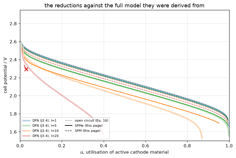
I =    1: DFN march ended on utilisation at u = 1.000; SPMe collector salt reaches zero never
I =    5: DFN march ended on utilisation at u = 1.000; SPMe collector salt reaches zero never
I =   10: DFN march ended on potential at u = 0.871; SPMe collector salt reaches zero never
I =   20: DFN march ended on newton at u = 0.397; SPMe collector salt reaches zero at u = 0.030
What the electrolyte correction actually is
The SPMe’s whole content beyond the SPM is the profile \(\tilde c(x,t)\). Below, against the DFN’s electrolyte at mid-discharge on the same grid, compared cell by cell. The DFN states come from marches with every step split into four, the finest level of the time ladder in Validation.
def dfn_mid(I, refine):
    """DFN salt profile at u = U_MID, the observation time a step time of the march."""
    c = Cell(P, KAPPA, *GRID)
    _, r = dfn_at(c, I, [U_MID], refine=refine)
    t_mid = next(iter(r["snaps"]))
    return t_mid, c.unpack(r["snaps"][t_mid])[0]


DFN_MID = {(I, m): dfn_mid(I, m) for I in (1.0, 5.0) for m in (2, 4)}


def profile_dev(I, s=sp, refine=4):
    """Largest |c_SPMe - c_DFN| / c_0 over the cells at u = U_MID, and the two profiles."""
    t_mid, c_dfn = DFN_MID[(I, refine)]
    c_spme = P["c_0"] + s.profile([t_mid], I)[0]
    return float(np.max(np.abs(c_spme - c_dfn)) / P["c_0"]), c_dfn, c_spme


PROF = {I: profile_dev(I) for I in (1.0, 5.0)}
PROF2 = {I: profile_dev(I, refine=2)[0] for I in (1.0, 5.0)}
fig, axes = plt.subplots(1, 2, figsize=(8.6, 3.6), sharex=True)
for ax, I in zip(axes, (1.0, 5.0)):
    dev, c_dfn, c_spme = PROF[I]
    ax.plot(1e6 * cell.x_c, c_dfn, color="tab:blue", lw=2.6, alpha=0.45, label="DFN (J3.4)")
    ax.plot(1e6 * sp.x_c, c_spme, "k-", lw=1.4, label=r"$c_0 + \tilde{c}$ (SPMe)")
    ax.axvline(1e6 * P["delta_s"], color="0.6", lw=0.8, ls=":")
    ax.set(xlabel=r"$x$ / $\mu$m", title=f"I = {I:g} A/m$^2$, u = {U_MID}")
    ax.text(0.03, 0.06, f"max dev {100 * dev:.2f} % of $c_0$", transform=ax.transAxes, fontsize=8)
axes[0].set_ylabel("salt concentration / mol m$^{-3}$")
axes[0].legend(fontsize=8)
fig.tight_layout()
plt.show()
claims.value("profile_dev_I1_frac", PROF[1.0][0])
claims.value("profile_dev_I5_frac", PROF[5.0][0])
print(f"largest profile deviation: {100 * PROF[1.0][0]:.3f} % of c_0 at I = 1, "
      f"{100 * PROF[5.0][0]:.2f} % at I = 5; with steps split into two instead of four: "
      f"{100 * PROF2[1.0]:.3f} % and {100 * PROF2[5.0]:.2f} %")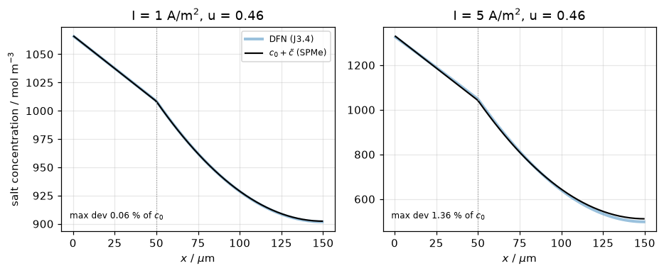
largest profile deviation: 0.057 % of c_0 at I = 1, 1.36 % at I = 5; with steps split into two instead of four: 0.057 % and 1.36 %display(Markdown(
f"At $I=1$ the first-order profile is the profile, to {100 * PROF[1.0][0]:.2f} % of $c_0$. At "
f"$I=5$ the shape is right but the linearisation strain is visible, "
f"{100 * PROF[5.0][0]:.1f} % of $c_0$: the SPMe carries the transference number at $c_0$ "
f"and a migration flux from the uniform leading-order reaction, while the DFN's reaction "
f"and $t^0_+$ follow the depleting salt."))At \(I=1\) the first-order profile is the profile, to 0.06 % of \(c_0\). At \(I=5\) the shape is right but the linearisation strain is visible, 1.4 % of \(c_0\): the SPMe carries the transference number at \(c_0\) and a migration flux from the uniform leading-order reaction, while the DFN’s reaction and \(t^0_+\) follow the depleting salt.
Validation
Everything here is model against model; the deviation convention is (reduced − full), in mV, with the full model the J3.4 DFN. In order:
- The paper’s arithmetic, Tables II and III recomputed from Table I (done above, under The data).
- An exact solution for the SPMe operator. The quasi-steady correction is piecewise quadratic in closed form; the pymrm solution must converge to it at second order. The backward-Euler march must converge to the exact-in-time modal solution at first order, and salt must be conserved.
- The asymptotic error scaling, the paper’s central claim. RMS voltage error against the DFN over a ladder of currents halving from 4 to 1/8 A/m², each case on matched grids, with the DFN reference’s own time and space error measured on every rung. The order comes from successive differences of the error along the ladder (
pymrm.checks.observed_orders, with \(1/I\) as the resolution). - What the scaling resolves: each correction term mis-scaled or deleted in turn, and a shared parameter moved.
- Identities: coulomb counting on the DFN, and the one restriction
bv_invertcarries.
A note on what the SPM’s order means. On this cell \(\kappa\) and \(D\) are constants and the first-order electrolyte perturbation is linear in \(I\), so the ohmic and quasi-steady concentration corrections the SPM omits are exactly proportional to \(I\): its order 1 is close to structural and is not independent evidence. Only the SPMe order is a test.
# ---- 2. the SPMe operator against the closed form, the march and salt ----------
OP_LEVELS = (12, 24, 48, 96)


def operator_metrics(**kw):
    S = {n: SPMe(P, KAPPA, n, 2 * n, **kw) for n in OP_LEVELS}
    rel = {}
    for n, s in S.items():
        exact = s.steady_closed_form(1.0)
        rel[n] = float(np.abs(s.steady(1.0) - exact).max() / np.ptp(exact))
    # end-face values: the same two positions on every grid
    ends = lambda n: np.array([S[n].wall(S[n].steady(1.0), 1.0)[0], S[n].collector(S[n].steady(1.0))[0]])
    o = observed_orders(ends, OP_LEVELS)
    fine = abs(np.abs(ends(96) - ends(48)).max()) / (96 * EPS * np.abs(ends(96)).max())
    return {"spme_steady_op_rel_err": rel[24], "spme_steady_op_order_min": min(o["orders"]),
            "spme_steady_op_order_max": max(o["orders"]), "spme_steady_finest_over_roundoff": fine,
            "_rel": rel, "_o": o}


OPM = operator_metrics()
for n in OP_LEVELS:
    print(f"steady SPMe vs closed-form quadratic, grid {n}+{2 * n}: max|dc|/amplitude = "
          f"{OPM['_rel'][n]:.2e}")
print(f"orders of the end-face values from successive differences: "
      + ", ".join(f"{x:.3f}" for x in OPM["_o"]["orders"]))
claims.value("spme_steady_op_rel_err", OPM["spme_steady_op_rel_err"])
claims.bound("spme_steady_op_order_min", OPM["spme_steady_op_order_min"], min=1.8, max=2.2,
             basis="theory", note="cell-centred diffusion with harmonic face means: order 2")
claims.bound("spme_steady_op_order_max", OPM["spme_steady_op_order_max"], min=1.8, max=2.2,
             basis="theory", note="as spme_steady_op_order_min")
claims.bound("spme_steady_finest_over_roundoff", OPM["spme_steady_finest_over_roundoff"], min=1e3,
             basis="theory", note="finest difference over n eps |c~|")

TAU_E = (P["delta_s"] + P["delta_c"]) ** 2 / P["D"]
T_EARLY = 0.05 * TAU_E                  # inside the transient, where the time error lives
NT_LEVELS = (50, 100, 200, 400)


def march_metrics(levels=NT_LEVELS, ratio=None, s=sp, assume_order=None):
    exact = s.profile([T_EARLY], 1.0)[0]
    o = observed_orders(lambda n: s.march(T_EARLY, 1.0, n)[-1], levels)
    if ratio is not None:                     # break rows: the same ladder read with another ratio
        vals = o["values"]
        o["orders"] = orders_with_ratio(vals, ratio)
        o["extrapolated"] = vals[-1] + (vals[-1] - vals[-2]) / (ratio ** o["orders"][-1] - 1)
    if assume_order is not None:              # break rows: extrapolated with a wrong order
        vals = o["values"]
        o["extrapolated"] = vals[-1] + (vals[-1] - vals[-2]) / (2.0 ** assume_order - 1)
    return {"spme_march_order_min": min(o["orders"]), "spme_march_order_max": max(o["orders"]),
            "spme_march_extrap_vs_exact": float(np.abs(o["extrapolated"] - exact).max()
                                                / np.abs(exact).max()), "_o": o}


MAR = march_metrics()
print(f"\nbackward Euler at t = {T_EARLY:.1f} s (0.05 tau_e), I = 1: orders "
      + ", ".join(f"{x:.3f}" for x in MAR["_o"]["orders"])
      + f"; extrapolated profile against the modal solution, relative to its largest value: "
        f"below 1e-4 (here {MAR['spme_march_extrap_vs_exact']:.1e})")
claims.bound("spme_march_order_min", MAR["spme_march_order_min"], min=0.9, max=1.1, basis="theory",
             note="backward Euler with equal steps: order 1")
claims.bound("spme_march_order_max", MAR["spme_march_order_max"], min=0.9, max=1.1, basis="theory",
             note="as spme_march_order_min")
claims.bound("spme_march_extrap_vs_exact", MAR["spme_march_extrap_vs_exact"], max=1e-4,
             basis="theory", note="Richardson remainder of a first-order march at 400 steps, "
                                  "second order in the step")


def salt_metrics(s=sp, I=1.0):
    t = (np.linspace(0.05, 0.85, 161) - P["u_0"]) * t_full(P) / I
    salt = (s.profile(t, I) * (s.eps * s.dx)).sum(axis=1)
    return {"salt_conservation_spme": float(np.abs(salt).max() / (P["c_0"] * np.sum(s.eps * s.dx)))}


SALT = salt_metrics()
claims.bound("salt_conservation_spme", SALT["salt_conservation_spme"], max=1e-11, basis="identity",
             note="largest |sum(eps dx c~)| over the I = 1 discharge, relative to the cell's salt; "
                  "the forcing of the constant mode is round-off, and it acts for the whole "
                  "discharge")
print(f"salt in the SPMe over the I = 1 discharge: below 1e-11 of the inventory "
      f"(here {SALT['salt_conservation_spme']:.1e})")
steady SPMe vs closed-form quadratic, grid 12+24: max|dc|/amplitude = 1.42e-04
steady SPMe vs closed-form quadratic, grid 24+48: max|dc|/amplitude = 3.53e-05
steady SPMe vs closed-form quadratic, grid 48+96: max|dc|/amplitude = 8.80e-06
steady SPMe vs closed-form quadratic, grid 96+192: max|dc|/amplitude = 2.19e-06
orders of the end-face values from successive differences: 2.000, 2.000
backward Euler at t = 150.0 s (0.05 tau_e), I = 1: orders 0.991, 0.995; extrapolated profile against the modal solution, relative to its largest value: below 1e-4 (here 2.7e-06)
salt in the SPMe over the I = 1 discharge: below 1e-11 of the inventory (here 9.0e-13)3. The asymptotic error scaling
For every current of the ladder the DFN is marched three times, with every step split into 1, 2 and 4; the comparison utilisations \(u = 0.05, 0.055, \dots, 0.85\) are step times at every level. Backward Euler is first order, so the time-extrapolated reference is \(2V_4 - V_2\), and the difference of the two extrapolations from \((1,2)\) and \((2,4)\) bounds what is left. Space is measured on its own ladder, 24 + 48, 48 + 96 and 96 + 192 cells, with the time steps fixed: once on the DFN alone, and once on the measured error, both models on the same grid. The SPMe needs no time ladder: its modal solution is exact in time.
SWEEP_I = (4.0, 2.0, 1.0, 0.5, 0.25, 0.125)
LEVELS_I = tuple(1.0 / I for I in SWEEP_I)                # 1/I as the resolution: 0.25 ... 8
UGRID = np.linspace(0.05, 0.85, 161)
REFINE = (1, 2, 4)
SPACE = (12, 24, 48, 96)


def spme_ladder(**kw):
    """The SPMe on every grid of the space ladder."""
    return {n: SPMe(P, KAPPA, n, 2 * n, **kw) for n in SPACE}


SPM_SPACE = spme_ladder()


def richardson(vals, levels=SPACE):
    """Extrapolation from the three finest levels, the RMS distance to the one from the
    three coarsest (an upper estimate of what the first leaves), and the finest order."""
    hi = observed_orders(lambda n: vals[n], levels[1:])
    lo = observed_orders(lambda n: vals[n], levels[:-1])
    return hi["extrapolated"], rms(hi["extrapolated"] - lo["extrapolated"]), hi["orders"][0]


def dfn_reference(I, kappa=KAPPA, refine=REFINE, space=SPACE):
    """Time ladder on the production grid and space ladder at the base steps; the
    reference adds both extrapolations to the production value."""
    out = {"V": {}, "fail": 0, "runs": {}}
    for m in refine:
        c = Cell(P, kappa, *GRID)
        out["V"][m], out["runs"][m] = dfn_at(c, I, UGRID, refine=m)
        out["fail"] += len(c.failures)
    V1, V2, V4 = (out["V"][m] for m in refine)
    out["order_t"] = observed_orders(lambda m: out["V"][m], refine)["orders"][0]
    out["t_ref"] = out["ref"] = 2 * V4 - V2                    # backward Euler: order 1
    out["t_rem"] = rms((2 * V4 - V2) - (2 * V2 - V1)) / 3     # second-order remainder of (2, 4)
    if space:
        out["Vx"] = {n: (V1 if n == GRID[0] else dfn_at(Cell(P, kappa, n, 2 * n), I, UGRID)[0])
                     for n in space}
        out["x_ext"], out["x_rem"], out["order_x"] = richardson(out["Vx"], space)
        out["ref"] = out["t_ref"] + (out["x_ext"] - V1)
    return out


REF = {I: dfn_reference(I) for I in SWEEP_I}
print("DFN reference, potentials in microvolts (RMS over the comparison points):")
print(f"{'I':>6}{'failed':>8}{'time order':>12}{'space order':>13}{'time error':>12}"
      f"{'space error':>13}   left after extrapolation")
print(f"{'':>6}{'solves':>8}{'':>12}{'':>13}{'at 1 step':>12}{'at 48 + 96':>13}")
for I in SWEEP_I:
    R = REF[I]
    print(f"{I:>6g}{R['fail']:>8d}{R['order_t']:>12.3f}{R['order_x']:>13.3f}"
          f"{1e6 * rms(R['V'][1] - R['t_ref']):>12.4f}{1e6 * rms(R['Vx'][GRID[0]] - R['x_ext']):>13.4f}"
          f"   (here {1e6 * (R['t_rem'] + R['x_rem']):.1e})")
DFN reference, potentials in microvolts (RMS over the comparison points):
I failed time order space order time error space error left after extrapolation
solves at 1 step at 48 + 96
4 0 1.040 2.000 42.1860 1.8458 (here 3.1e-01)
2 0 1.187 2.000 5.1334 0.8899 (here 9.1e-02)
1 0 1.087 2.000 0.9281 0.4390 (here 7.1e-03)
0.5 0 1.106 2.000 0.2052 0.2182 (here 1.6e-03)
0.25 0 1.001 2.000 0.0471 0.1088 (here 5.4e-04)
0.125 0 0.985 2.000 0.0112 0.0543 (here 1.7e-04)def spme_limit(I, models=SPM_SPACE, vkw=None):
"""SPMe potential on every grid of the ladder (exact in time) and its space limit."""
Ve = {n: models[n].v_at(UGRID, I, **(vkw or {})) for n in SPACE}
ext, rem, order = richardson(Ve)
return {"ext": ext, "rem": rem, "order": order, "Ve": Ve}
def error_metrics(REF=REF, spm_P=P, models=SPM_SPACE, vkw=None, ratio=None):
"""RMS errors of the SPM and the SPMe against the DFN on every rung, both models at
their space and time limits, and the orders along the current ladder."""
LIM = {I: spme_limit(I, models, vkw) for I in SWEEP_I}
e_spm = {I: rms(v_spm(UGRID, I, spm_P) - REF[I]["ref"]) for I in SWEEP_I}
e_spme = {I: rms(LIM[I]["ext"] - REF[I]["ref"]) for I in SWEEP_I}
if ratio is None:
o_spm = observed_orders(lambda n: e_spm[1.0 / n], LEVELS_I)
o_spme = observed_orders(lambda n: e_spme[1.0 / n], LEVELS_I)
else:
o_spm = {"orders": orders_with_ratio([e_spm[I] for I in SWEEP_I], ratio)}
o_spme = {"orders": orders_with_ratio([e_spme[I] for I in SWEEP_I], ratio)}
floor = lambda I: len(REF[I]["runs"][4]["t"]) * EPS * 3.0 + 1e-9 * RTF
return {"rms_spm_I1_mV": 1e3 * e_spm[1.0], "rms_spme_I1_mV": 1e3 * e_spme[1.0],
"rms_spm_I4_mV": 1e3 * e_spm[4.0], "rms_spme_I4_mV": 1e3 * e_spme[4.0],
"rms_spme_I0125_mV": 1e3 * e_spme[0.125],
"ratio_spm_over_spme_I1": e_spm[1.0] / e_spme[1.0],
"spm_order_min": min(o_spm["orders"]), "spm_order_max": max(o_spm["orders"]),
"spme_order_I05_I0125": o_spme["orders"][3], "spme_order_I1_I025": o_spme["orders"][2],
"spme_order_I2_I05": o_spme["orders"][1], "spme_order_I4_I1": o_spme["orders"][0],
"spm_finest_over_roundoff": abs(e_spm[0.25] - e_spm[0.125]) / floor(0.125),
"spme_finest_over_roundoff": abs(e_spme[0.25] - e_spme[0.125]) / floor(0.125),
"spme_order_rises_with_current_count": int(np.sum(-np.diff(o_spme["orders"]) > 0)),
"_e_spm": e_spm, "_e_spme": e_spme, "_o_spm": o_spm["orders"],
"_o_spme": o_spme["orders"], "_LIM": LIM}
ERR = error_metrics()
E48 = {I: rms(SPM_SPACE[GRID[0]].v_at(UGRID, I) - REF[I]["t_ref"]) for I in SWEEP_I}
print(f"{'I / A/m2':>9}{'C_e':>9}{'SPM RMS/mV':>12}{'SPMe RMS/mV':>14}{'ratio':>8}"
f"{'SPMe, both on 48 + 96':>24}")
for I in SWEEP_I:
print(f"{I:>9.3f}{c_e(I, P):>9.4f}{1e3 * ERR['_e_spm'][I]:>12.4f}"
f"{1e3 * ERR['_e_spme'][I]:>14.6f}{ERR['_e_spm'][I] / ERR['_e_spme'][I]:>8.0f}"
f"{1e3 * E48[I]:>24.6f}")
print("\norders from successive differences, triples from high to low current "
"(4-2-1, 2-1-0.5, 1-0.5-0.25, 0.5-0.25-0.125):")
print(" SPM :", " ".join(f"{x:.3f}" for x in ERR["_o_spm"]))
print(" SPMe:", " ".join(f"{x:.3f}" for x in ERR["_o_spme"]))
print("SPMe space orders on the ladder 24, 48, 96 (one per current): "
+ ", ".join(f"{ERR['_LIM'][I]['order']:.3f}" for I in SWEEP_I))
print(f"smallest error difference over its round-off and newton floor: SPM above 1e3 "
f"(here {ERR['spm_finest_over_roundoff']:.1e}), SPMe above 1e3 (here "
f"{ERR['spme_finest_over_roundoff']:.1e})")
for k in ("rms_spm_I1_mV", "rms_spme_I1_mV", "rms_spm_I4_mV", "rms_spme_I4_mV", "rms_spme_I0125_mV"):
claims.value(k, ERR[k], unit="mV")
claims.value("ratio_spm_over_spme_I1", ERR["ratio_spm_over_spme_I1"])
claims.bound("spm_order_min", ERR["spm_order_min"], min=0.9, max=1.1, basis="theory",
note="SPM error O(C_e): order 1 along the current ladder")
claims.bound("spm_order_max", ERR["spm_order_max"], min=0.9, max=1.1, basis="theory",
note="as spm_order_min")
claims.bound("spme_order_I05_I0125", ERR["spme_order_I05_I0125"], min=1.8, max=2.2, basis="theory",
note="SPMe error O(C_e^2): order 2 as C_e -> 0, the lowest triple of the ladder")
for k in ("spme_order_I1_I025", "spme_order_I2_I05", "spme_order_I4_I1"):
claims.value(k, ERR[k])
N_RISE = claims.count("spme_order_rises_with_current_count", -np.diff(ERR["_o_spme"]), 0.0,
min_margin=0.01, note="successive SPMe triples (high to low current) whose "
"order falls; margin = smallest step")
claims.bound("spm_finest_over_roundoff", ERR["spm_finest_over_roundoff"], min=1e3, basis="theory",
note="smallest error difference over n_steps eps V + 1e-9 RT/F")
claims.bound("spme_finest_over_roundoff", ERR["spme_finest_over_roundoff"], min=1e3, basis="theory",
note="as spm_finest_over_roundoff") I / A/m2 C_e SPM RMS/mV SPMe RMS/mV ratio SPMe, both on 48 + 96
4.000 0.0613 49.2345 1.507519 33 1.508320
2.000 0.0306 24.2976 0.231547 105 0.231856
1.000 0.0153 12.1379 0.045142 269 0.045251
0.500 0.0077 6.0739 0.010124 600 0.010163
0.250 0.0038 3.0391 0.002419 1256 0.002434
0.125 0.0019 1.5202 0.000593 2563 0.000600
orders from successive differences, triples from high to low current (4-2-1, 2-1-0.5, 1-0.5-0.25, 0.5-0.25-0.125):
SPM : 1.036 1.004 0.999 0.999
SPMe: 2.775 2.412 2.184 2.077
SPMe space orders on the ladder 24, 48, 96 (one per current): 2.000, 2.000, 2.000, 2.000, 2.000, 2.000
smallest error difference over its round-off and newton floor: SPM above 1e3 (here 4.6e+07), SPMe above 1e3 (here 5.5e+04)def budget_metrics(REF=REF, space=True, n=GRID[0]):
"""What is left of the discretisation error in each model, over the SPMe error, per rung.
Without ``space`` the models are read on the ``n`` grid without the space
extrapolation, and their space error at ``n`` is what is left."""
dfn_err, e_unc = {}, {}
for I in SWEEP_I:
R, L = REF[I], ERR["_LIM"][I]
x_left = R["x_rem"] if space else rms(R["Vx"][n] - R["x_ext"])
e_left = L["rem"] if space else rms(L["Ve"][n] - L["ext"])
dfn_err[I] = (R["t_rem"] + x_left) / ERR["_e_spme"][I]
e_unc[I] = e_left / ERR["_e_spme"][I]
return {"dfn_ref_error_over_spme_error_max": max(dfn_err.values()),
"spme_error_space_uncertainty_max": max(e_unc.values()),
"dfn_time_order_min": min(REF[I]["order_t"] for I in SWEEP_I),
"dfn_time_order_max": max(REF[I]["order_t"] for I in SWEEP_I),
"dfn_failed_solves_sweep": sum(REF[I]["fail"] for I in SWEEP_I),
"_dfn_err": dfn_err, "_e_unc": e_unc}
BUD = budget_metrics()
print("what is left after extrapolation, over the SPMe error it is compared with:")
for I in SWEEP_I:
print(f" I = {I:<6g} DFN reference (here {BUD['_dfn_err'][I]:.1e}), "
f"SPMe (here {BUD['_e_unc'][I]:.1e})")
print(f"largest over the rungs: DFN below 0.01 (here {BUD['dfn_ref_error_over_spme_error_max']:.1e}), "
f"SPMe below 0.01 (here {BUD['spme_error_space_uncertainty_max']:.1e})")
print(f"newton solves that failed in the {3 * len(SWEEP_I)} sweep marches, I down to "
f"{min(SWEEP_I)} A/m2: {BUD['dfn_failed_solves_sweep']}")
claims.bound("dfn_ref_error_over_spme_error_max", BUD["dfn_ref_error_over_spme_error_max"], max=0.01,
basis="chosen", note="time and space remainders of the extrapolated DFN reference over "
"the SPMe error it is compared with, largest over the rungs; a "
"hundredth moves an order by at most about 0.03")
claims.bound("spme_error_space_uncertainty_max", BUD["spme_error_space_uncertainty_max"], max=0.01,
basis="chosen", note="space remainder of the extrapolated SPMe over its error, largest "
"over the rungs")
claims.bound("dfn_time_order_min", BUD["dfn_time_order_min"], min=0.8, max=1.2, basis="theory",
note="backward Euler on a nested time grid: order 1; the coarsest level is "
"pre-asymptotic at the middle currents, and the remainder estimate covers it")
claims.bound("dfn_time_order_max", BUD["dfn_time_order_max"], min=0.8, max=1.2, basis="theory",
note="as dfn_time_order_min")
claims.exact("dfn_failed_solves_sweep", BUD["dfn_failed_solves_sweep"])
fig, ax = plt.subplots(figsize=(6.2, 4.2))
Iv = np.array(SWEEP_I)
es = 1e3 * np.array([ERR["_e_spm"][I] for I in SWEEP_I])
ee = 1e3 * np.array([ERR["_e_spme"][I] for I in SWEEP_I])
ax.loglog(Iv, es, "o-", color="tab:red", label="SPM")
ax.loglog(Iv, ee, "s-", color="tab:blue", label="SPMe")
ref_I = np.array([Iv.min(), Iv.max()])
ax.loglog(ref_I, es[-1] * ref_I / Iv[-1], ":", color="tab:red", lw=1, label="slope 1")
ax.loglog(ref_I, ee[-1] * (ref_I / Iv[-1]) ** 2, ":", color="tab:blue", lw=1, label="slope 2")
ax.set(xlabel="discharge current density $I$ / A m$^{-2}$", ylabel="RMS voltage error vs DFN / mV",
title="the error scaling the asymptotics promise")
ax.legend(fontsize=8)
fig.tight_layout()
plt.show()what is left after extrapolation, over the SPMe error it is compared with:
I = 4 DFN reference (here 2.0e-04), SPMe (here 6.2e-10)
I = 2 DFN reference (here 3.9e-04), SPMe (here 5.2e-10)
I = 1 DFN reference (here 1.6e-04), SPMe (here 4.9e-11)
I = 0.5 DFN reference (here 1.6e-04), SPMe (here 6.5e-10)
I = 0.25 DFN reference (here 2.2e-04), SPMe (here 1.8e-09)
I = 0.125 DFN reference (here 2.9e-04), SPMe (here 3.7e-09)
largest over the rungs: DFN below 0.01 (here 3.9e-04), SPMe below 0.01 (here 3.7e-09)
newton solves that failed in the 18 sweep marches, I down to 0.125 A/m2: 0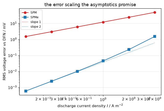
display(Markdown(
    f"**What the ladder says.** The SPM error falls in proportion to the current, orders "
    f"{ERR['spm_order_min']:.3f} to {ERR['spm_order_max']:.3f}. The SPMe error falls as the "
    f"square as the current goes to zero: the order of the lowest triple is {ERR['spme_order_I05_I0125']:.2f}, and it rises "
    f"with current at every step of the ladder, to {ERR['spme_order_I1_I025']:.2f}, "
    f"{ERR['spme_order_I2_I05']:.2f} and {ERR['spme_order_I4_I1']:.2f} for the triples above, "
    f"as the terms of higher order in $\\mathcal{{C}}_e$ grow. The $O(\\mathcal{{C}}_e)$ and "
    f"$O(\\mathcal{{C}}_e^2)$ the paper derives are reproduced; the higher-current orders are "
    f"pre-asymptotic, not a contradiction. At $I=1$ A/m² the errors are "
    f"{ERR['rms_spm_I1_mV']:.2f} mV (SPM) and {ERR['rms_spme_I1_mV']:.4f} mV (SPMe), a factor "
    f"{ERR['ratio_spm_over_spme_I1']:.0f}. The DFN reference's own time and space error is below 0.01 of the SPMe error it is "
    f"compared with on every rung (here at most {BUD['dfn_ref_error_over_spme_error_max']:.1e}); at the lowest current the SPMe error is "
    f"{1e3 * ERR['rms_spme_I0125_mV']:.2f} µV."))
What the ladder says. The SPM error falls in proportion to the current, orders 0.999 to 1.036. The SPMe error falls as the square as the current goes to zero: the order of the lowest triple is 2.08, and it rises with current at every step of the ladder, to 2.18, 2.41 and 2.78 for the triples above, as the terms of higher order in \(\mathcal{C}_e\) grow. The \(O(\mathcal{C}_e)\) and \(O(\mathcal{C}_e^2)\) the paper derives are reproduced; the higher-current orders are pre-asymptotic, not a contradiction. At \(I=1\) A/m² the errors are 12.14 mV (SPM) and 0.0451 mV (SPMe), a factor 269. The DFN reference’s own time and space error is below 0.01 of the SPMe error it is compared with on every rung (here at most 3.9e-04); at the lowest current the SPMe error is 0.59 µV.
4. What the scaling resolves, and what it does not
A scaling test is only as strong as the terms it can see. Each of the four first-order corrections is now mis-scaled or deleted in turn, on the same electrolyte solution and against the same DFN reference, so the table below isolates the voltage assembly alone.
PRE0 = pre0(P)
MUT = [("baseline (canonical SPMe)", {}),
       ("ohmic delta_c/3 -> delta_c/2.7  (10 %)", {"ohm_div": 2.7}),
       ("concentration factor 2 -> 2.2  (10 %)", {"conc_fac": 2.2}),
       ("electrode-averaged exchange current deleted", {"pre": PRE0}),
       ("anode overpotential at c_0, not c(0)", {"c_anode": P["c_0"]})]


def mutation_metrics(MUT=MUT, ratio=None):
    E = {name: error_metrics(vkw=kw, ratio=ratio) for name, kw in MUT}
    base = E[MUT[0][0]]["_e_spme"][1.0]
    r = {name: E[name]["_e_spme"][1.0] / base for name, _ in MUT}
    return {"mut_ohm_error_ratio_I1": r[MUT[1][0]], "mut_conc_error_ratio_I1": r[MUT[2][0]],
            "mut_exchange_avg_error_ratio_I1": r[MUT[3][0]], "mut_anode_error_ratio_I1": r[MUT[4][0]],
            "mut_ohm_order_lowest": E[MUT[1][0]]["spme_order_I05_I0125"],
            "mut_conc_order_lowest": E[MUT[2][0]]["spme_order_I05_I0125"],
            "mut_anode_order_lowest": E[MUT[4][0]]["spme_order_I05_I0125"], "_E": E}


MUTM = mutation_metrics()
print(f"{'variant':>44}{'RMS(I=1)/mV':>13}{'x base':>8}{'orders, high to low current':>34}")
for name, _ in MUT:
    e = MUTM["_E"][name]
    print(f"{name:>44}{1e3 * e['_e_spme'][1.0]:>13.5f}"
          f"{e['_e_spme'][1.0] / ERR['_e_spme'][1.0]:>8.4f}   " + "".join(f"{x:>7.3f}" for x in e["_o_spme"]))
for k in ("mut_ohm_error_ratio_I1", "mut_conc_error_ratio_I1", "mut_exchange_avg_error_ratio_I1",
          "mut_anode_error_ratio_I1"):
    claims.value(k, MUTM[k])
claims.bound("mut_ohm_order_lowest", MUTM["mut_ohm_order_lowest"], min=0.8, max=1.2, basis="theory",
             note="an uncancelled O(C_e) remainder: order 1 as C_e -> 0")
claims.bound("mut_conc_order_lowest", MUTM["mut_conc_order_lowest"], min=0.8, max=1.2, basis="theory",
             note="as mut_ohm_order_lowest")
claims.value("mut_anode_order_lowest", MUTM["mut_anode_order_lowest"])
variant RMS(I=1)/mV x base orders, high to low current
baseline (canonical SPMe) 0.04514 1.0000 2.775 2.412 2.184 2.077
ohmic delta_c/3 -> delta_c/2.7 (10 %) 0.44413 9.8386 -0.373 0.690 0.924 0.978
concentration factor 2 -> 2.2 (10 %) 0.67482 14.9491 -0.136 0.792 0.948 0.985
electrode-averaged exchange current deleted 0.04515 1.0001 2.775 2.412 2.184 2.077
anode overpotential at c_0, not c(0) 0.04953 1.0972 2.756 1.813 1.817 1.902display(Markdown(
f"Two of the four terms are resolved sharply. A 10 % error in the ohmic or the concentration "
f"coefficient multiplies the $I=1$ error by {MUTM['mut_ohm_error_ratio_I1']:.1f} and "
f"{MUTM['mut_conc_error_ratio_I1']:.1f}, and takes the order of the lowest triple to "
f"{MUTM['mut_ohm_order_lowest']:.2f} and {MUTM['mut_conc_order_lowest']:.2f}: the uncancelled "
f"$O(\\mathcal{{C}}_e)$ remainder then dominates, which is the failure the asymptotics "
f"predict. The other two are **not** resolved on this cell. Deleting the electrode-averaged "
f"exchange-current correction (their Eqs. 48n and 48o) changes the error by "
f"{100 * (MUTM['mut_exchange_avg_error_ratio_I1'] - 1):.2f} %: for a 1:1 salt at "
f"$c_0$ = {P['c_0']:.0f} against $c_{{\\max}}$ = {P['c_max']:.0f} mol/m³ the cathode average of "
f"the prefactor is indistinguishable from its value at $c_0$, so a sign error in that term "
f"would pass. Evaluating the anode overpotential at $c_0$ instead of $c(0)$ changes the error "
f"by {100 * (MUTM['mut_anode_error_ratio_I1'] - 1):.0f} % and leaves the lowest order at "
f"{MUTM['mut_anode_order_lowest']:.2f}: visible, not sharp. Read the ladder as verifying the "
f"ohmic and concentration corrections, and as bounding, not verifying, the exchange-current "
f"average and the anode term."))Two of the four terms are resolved sharply. A 10 % error in the ohmic or the concentration coefficient multiplies the \(I=1\) error by 9.8 and 14.9, and takes the order of the lowest triple to 0.98 and 0.99: the uncancelled \(O(\mathcal{C}_e)\) remainder then dominates, which is the failure the asymptotics predict. The other two are not resolved on this cell. Deleting the electrode-averaged exchange-current correction (their Eqs. 48n and 48o) changes the error by 0.01 %: for a 1:1 salt at \(c_0\) = 1000 against \(c_{\max}\) = 3920 mol/m³ the cathode average of the prefactor is indistinguishable from its value at \(c_0\), so a sign error in that term would pass. Evaluating the anode overpotential at \(c_0\) instead of \(c(0)\) changes the error by 10 % and leaves the lowest order at 1.90: visible, not sharp. Read the ladder as verifying the ohmic and concentration corrections, and as bounding, not verifying, the exchange-current average and the anode term.
5. Identities
Coulomb counting. Summing the DFN’s solid balance over the cathode and using the charge balance gives \(u = u_0 + It/\big(F(1-\epsilon)c_T\delta_c\big)\) at every step: Marquis et al.’s Eq. 32 (the electrode-averaged solid concentration has no first-order correction) holding exactly at constant current. It is what lets the SPM and the SPMe run on \(u(t)\) without a particle.
The restriction bv_invert carries. Writing \(z=e^{\alpha f\eta'}\) turns Eq. 17 into a quadratic in \(z\) only when its two exponents are \(+\alpha_a f\eta'\) and \(-\alpha_c f\eta'\) with \(\alpha_a=\alpha_c\). The closed form is fed back through Eq. 17, at Doyle’s own symmetric pair and at two asymmetric pairs a reader might plausibly have, with the true overpotential the one root of Eq. 17 on \(\pm 3\) V; bv_invert itself refuses the asymmetric pairs.
def coulomb_metrics(r=REF[1.0]["runs"][1]):
    return {"coulomb_identity_dev": float(np.max(np.abs(r["u"] - u_of_t(r["t"], 1.0, P))))}


COUL = coulomb_metrics()
claims.bound("coulomb_identity_dev", COUL["coulomb_identity_dev"], max=1e-12, basis="identity",
             note="state utilisation against coulomb counting over the I = 1 sweep march")
print(f"DFN coulomb-counting identity at I = 1: max |u - (u_0 + I t / Q)| below 1e-12 "
      f"(here {COUL['coulomb_identity_dev']:.1e}, {len(REF[1.0]['runs'][1]['t'])} steps)")

CS_T = 0.30 * P["c_T"]                  # a mid-discharge surface concentration
PAIRS = ((0.5, 0.5), (0.3, 0.7), (0.4, 0.6))
I_TRY = (0.05, 0.5, 5.0)


def bv_metrics(pairs=PAIRS, pre_feedback=1.0):
    sym, asym, rows = 0.0, 0.0, []
    for aa, ac in pairs:
        Pa = dict(P, alpha_a=aa, alpha_c=ac)
        for i_t in I_TRY:
            eta_c = bv_eta(CS_T, i_t, PRE0, Pa, check=False)              # the unchecked formula
            f = lambda e: i_eq17(e, CS_T, PRE0, P, aa, ac) - i_t
            res = find_roots(f, -3.0, 3.0, n_scan=200)
            if len(res["roots"]) != 1:
                raise RuntimeError(res["message"])
            ratio = i_eq17(eta_c, CS_T, pre_feedback * PRE0, P, aa, ac) / i_t
            if aa == ac:
                sym = max(sym, abs(ratio - 1))
            else:
                asym = max(asym, abs(ratio - 1))
            rows.append((aa, ac, i_t, eta_c, res["roots"][0], ratio))
    try:
        bv_invert(CS_T, 0.5, PRE0, dict(P, alpha_a=0.3, alpha_c=0.7))
        refused = False
    except ValueError:
        refused = True
    return {"bv_invert_symmetric_max_current_dev": sym, "bv_invert_asymmetric_max_current_dev": asym,
            "bv_invert_refuses_asymmetric": refused, "_rows": rows}


BV = bv_metrics()
print(f"\n{'alpha_a':>9}{'alpha_c':>9}{'i / A m-2':>12}{'eta_closed/mV':>15}{'eta_true/mV':>13}"
      f"{'i recovered / i asked':>23}")
for aa, ac, i_t, ec, et, ratio in BV["_rows"]:
    print(f"{aa:>9.1f}{ac:>9.1f}{i_t:>12.2f}{1e3 * ec:>15.3f}{1e3 * et:>13.3f}{ratio:>23.4f}")
claims.bound("bv_invert_symmetric_max_current_dev", BV["bv_invert_symmetric_max_current_dev"],
             max=1e-12, basis="identity", note="closed form fed back through Eq. 17 at alpha_a = alpha_c")
claims.value("bv_invert_asymmetric_max_current_dev", BV["bv_invert_asymmetric_max_current_dev"])
claims.exact("bv_invert_refuses_asymmetric", BV["bv_invert_refuses_asymmetric"])
print(f"\nAt alpha_a = alpha_c the closed form reproduces the requested current to below 1e-12 "
      f"(here {BV['bv_invert_symmetric_max_current_dev']:.1e}).")
print(f"At alpha_a != alpha_c the unchecked formula delivers up to "
      f"{1 + BV['bv_invert_asymmetric_max_current_dev']:.0f} times the requested current, with a "
      f"finite, plausible overpotential that is not the root of Eq. 17; bv_invert raises instead "
      f"({BV['bv_invert_refuses_asymmetric']}).")
DFN coulomb-counting identity at I = 1: max |u - (u_0 + I t / Q)| below 1e-12 (here 3.3e-16, 320 steps)
alpha_a alpha_c i / A m-2 eta_closed/mV eta_true/mV i recovered / i asked
0.5 0.5 0.05 27.252 27.252 1.0000
0.5 0.5 0.50 27.318 27.318 1.0000
0.5 0.5 5.00 27.978 27.978 1.0000
0.3 0.7 0.05 45.419 27.253 1892.3843
0.3 0.7 0.50 45.530 27.331 190.2847
0.3 0.7 5.00 46.630 28.118 20.0695
0.4 0.6 0.05 34.065 27.252 837.6503
0.4 0.6 0.50 34.147 27.324 84.7609
0.4 0.6 5.00 34.973 28.045 9.4699
At alpha_a = alpha_c the closed form reproduces the requested current to below 1e-12 (here 5.5e-14).
At alpha_a != alpha_c the unchecked formula delivers up to 1892 times the requested current, with a finite, plausible overpotential that is not the root of Eq. 17; bv_invert raises instead (True).The break table
Each row injects one defect through an argument of the functions above (a parameter, a model option or a study setting) and recomputes the claims it reaches; a claim is caught when the defect fails its own check. Defects in the reduced models reuse the DFN reference; defects in the DFN rerun it.
# Marquis arithmetic: transcription defects in Table I and in the printed values


def marquis_counts(d):
    u = d["_units"]
    return {**d, "marquis_above_half_unit_count": int(np.sum(u > 0.5)),
            "marquis_below_half_unit_count": int(np.sum(u < -0.5)),
            "marquis_within_one_unit_count": int(np.sum(u < 1.0))}


run_row("Table I L_p 10 % high (data)", marquis_counts(marquis_metrics(dict(M, L_p=1.1 * M["L_p"]))))
run_row("Table I D_e_typ 10 % high (data)",
        marquis_counts(marquis_metrics(dict(M, D_e_typ=1.1 * M["D_e_typ"]))))
run_row("printed values rounded instead of truncated (data)",
        marquis_counts(marquis_metrics(M, stated={**STATED, **{
            k: round(v / UNIT[k]) * UNIT[k] for k, v in MQ["_der"].items()}})))
brk("Table III gamma_n row counted (data)", "marquis_tables_checked", MQ["marquis_tables_checked"] + 1)

# Table VI and the depletion current: parameter defects
P_D = dict(P, D=5.7e-12)
row = "D 7.5e-12 -> 5.7e-12 in the reductions (P)"
run_row(row, table6_metrics(P_D))
run_row("sigma 1.0e4 -> 1.0e2 (P)", table6_metrics(dict(P, sigma=1.0e2)))
run_row("k_2 x10 (P)", table6_metrics(dict(P, k_2=10 * P["k_2"])))
run_row("kappa from the Eq. 29 route (kappa)", table6_metrics(kappa=KAPPA_29))
sp_D = SPMe(P_D, KAPPA, *GRID)
brk(row, "spme_salt_exhausted_u_I20", spme_exhaustion_u(20.0, sp_D))
run_row(row, error_metrics(models={n: SPMe(P_D, KAPPA, n, 2 * n) for n in SPACE}))
for I, key in ((1.0, "profile_dev_I1_frac"), (5.0, "profile_dev_I5_frac")):
    brk(row, key, profile_dev(I, s=sp_D)[0])
sp_p = SPMe(P, KAPPA, *GRID, p_D=1.5)
for I, key in ((1.0, "profile_dev_I1_frac"), (5.0, "profile_dev_I5_frac")):
    brk("SPMe salt Bruggeman eps^1.5 (p_D)", key, profile_dev(I, s=sp_p)[0])
brk("SPMe salt Bruggeman eps^1.5 (p_D)", "spme_salt_exhausted_u_I20", spme_exhaustion_u(20.0, sp_p))

# the SPMe operator and its routes
run_row("arithmetic face mean in the SPMe (face_mean)", operator_metrics(face_mean="arithmetic"))
row = "finest rung repeats the one before (levels)"
brk(row, "spme_steady_finest_over_roundoff", 0.0)
brk(row, "spm_finest_over_roundoff", 0.0)
brk(row, "spme_finest_over_roundoff", 0.0)
run_row("march ladder 50, 100, 200, 400 read with ratio 3 (levels)", march_metrics(ratio=3.0))
run_row("march extrapolated as if second order (order)", march_metrics(assume_order=2.0))
sp_w = SPMe(P, KAPPA, *GRID, datum_factor=1.1)
row = "lithium-face datum x1.1 in the SPMe (datum_factor)"
run_row(row, salt_metrics(sp_w))
run_row(row, error_metrics(models=spme_ladder(datum_factor=1.1)))

# the reduced voltages: one term at a time, against the same reference
for name, kw in MUT[1:]:
    run_row(name + " (voltage)", {k: v for k, v in error_metrics(vkw=kw).items()
                                   if not k.startswith(("spm_", "rms_spm_I"))})
row = "SPM open-circuit potential 5 mV high (U_theta in v_spm)"
run_row(row, {k: v for k, v in error_metrics(spm_P=dict(P, U_theta=P["U_theta"] + 5e-3)).items()
              if k.startswith(("spm_", "rms_spm_I", "ratio"))})
row = "mutations sized 20 % instead of 10 % (study)"
_m20 = mutation_metrics([MUT[0], ("o", {"ohm_div": 2.4}), ("c", {"conc_fac": 2.4}),
                         ("e", {"pre": 0.01 * PRE0}), ("a", {"c_anode": 1.1 * P["c_0"]})])
run_row(row + ", prefactor at a hundredth", _m20)
run_row("orders read with ratio 3 (levels)", {k: v for k, v in mutation_metrics(ratio=3.0).items()
                                              if k.endswith("order_lowest")})

# the reference
run_row("both models read on 48 + 96 without space extrapolation (study)", budget_metrics(space=False))
_ot3 = [orders_with_ratio([REF[I]["V"][m] for m in REFINE], 3.0)[0] for I in SWEEP_I]
run_row("orders read with ratio 3 (levels)", {**error_metrics(ratio=3.0), "dfn_time_order_min": min(_ot3),
                                              "dfn_time_order_max": max(_ot3)})
row = "kappa raised in the SPMe's ohmic term only (kappa)"
run_row(row, kappa_metrics(k_spme=KAP_HI, R=REF[1.0]))
row = "kappa raised by twice the route gap in both models (kappa)"
run_row(row, kappa_metrics(k_spme=(1 + 2 * KAP_GAP) * KAPPA, k_dfn=(1 + 2 * KAP_GAP) * KAPPA))

# the DFN copy and its solves
run_row("arithmetic face mean in the DFN copy (face_mean)", j34_copy_metrics(face_mean="arithmetic"))
_c = Cell(P, KAPPA, *GRID)
_c.march(0.125, t_stop=0.02 * _c.t_full / 0.125, tol=1e-16, stop_on_failure=True)
brk("newton tol 1e-9 -> 1e-16, below round-off (tol)", "dfn_failed_solves_sweep", len(_c.failures))
_c = Cell(P, KAPPA, *GRID, ai_solid=1.1)
brk("pore-wall current x1.1 in the solid balance (ai_solid)", "coulomb_identity_dev",
    coulomb_metrics(_c.march(1.0, t_stop=0.1 * _c.t_full))["coulomb_identity_dev"])

# bv_invert
run_row("feedback with the prefactor 1 % high (pre)", bv_metrics(pre_feedback=1.01))
run_row("asymmetric pairs 0.45/0.55 and 0.4/0.6 (study)", bv_metrics(pairs=((0.5, 0.5), (0.45, 0.55),
                                                                          (0.4, 0.6))))
brk("bv_invert called with check=False (check)", "bv_invert_refuses_asymmetric", False)

# One line per claim: how many rows fail it, and the first of them.
by_claim = {}
for row_, metric, clean_v, broken, caught in BREAK:
    by_claim.setdefault(metric, []).append((row_, broken, caught))
print(f"{'claim':<40} {'clean':>12} {'rows':>4} {'fail':>4}  first failing row (its value)")
for metric, c in claims.metrics.items():
    rows_m = by_claim.get(metric, [])
    fails = [(r, b) for r, b, k in rows_m if k]
    shown = f"(here {c['value']:.1e})" if c["kind"] == "bound" else f"{float(c['value']):.5g}"
    first = (f"{fails[0][0]} ({float(fails[0][1]):.4g})" if fails
             else ("structural" if c.get("structural") else "NONE"))
    print(f"{metric[:40]:<40} {shown:>12} {len(rows_m):4d} {len(fails):4d}  {first}")
_caught = {mt for _, mt, _, _, k in BREAK if k}
_open = sorted(k for k in claims.metrics if k not in _caught and not claims.metrics[k].get("structural"))
print(f"\n{len(BREAK)} rows over {len(claims.metrics)} claims; {len(_caught)} claims are failed by at "
      f"least one row, {sum(bool(c.get('structural')) for c in claims.metrics.values())} structural; "
      f"open: {', '.join(_open) or 'none'}")
claim clean rows fail first failing row (its value)
marquis_tables_checked 21 4 1 Table III gamma_n row counted (data) (22)
marquis_tables_max_rel_dev 0.0012305 3 3 Table I L_p 10 % high (data) (0.09087)
marquis_C_e_recomputed 0.0041952 3 1 Table I D_e_typ 10 % high (data) (0.003814)
ce_text_vs_recomputed_rel 0.17742 3 2 Table I L_p 10 % high (data) (0.1409)
marquis_above_half_unit_count 3 3 3 Table I L_p 10 % high (data) (4)
marquis_below_half_unit_count 0 3 2 Table I L_p 10 % high (data) (9)
marquis_within_one_unit_count 21 3 1 Table I L_p 10 % high (data) (17)
j34_copy_max_rel_gap (here 0.0e+00) 1 1 arithmetic face mean in the DFN copy (face_mean) (0.002047)
Ce_doyle_at_I10 0.15316 4 1 D 7.5e-12 -> 5.7e-12 in the reductions (P) (0.2015)
Ce_at_I1 0.015316 4 1 D 7.5e-12 -> 5.7e-12 in the reductions (P) (0.02015)
Ce_at_I20 0.30633 4 1 D 7.5e-12 -> 5.7e-12 in the reductions (P) (0.4031)
kappa_hat_at_I1 10.403 4 1 kappa from the Eq. 29 route (kappa) (8.766)
kappa_hat_at_I10 1.0403 4 1 kappa from the Eq. 29 route (kappa) (0.8766)
kappa_hat_at_I20 0.52015 4 1 kappa from the Eq. 29 route (kappa) (0.4383)
C_r_doyle_at_I10 9.9592e-05 4 1 k_2 x10 (P) (9.959e-06)
table6_conditions_245_min_orders (here 4.2e+00) 4 1 sigma 1.0e4 -> 1.0e2 (P) (3.03)
Ce_equals_S_s_gap (here 0.0e+00) 4 0 structural
Ce_I10_within_printed_S_s 1 4 1 D 7.5e-12 -> 5.7e-12 in the reductions (P) (0)
I_depletion_Am2 10.24 4 1 D 7.5e-12 -> 5.7e-12 in the reductions (P) (7.783)
spme_salt_exhausted_u_I20 0.029829 2 1 SPMe salt Bruggeman eps^1.5 (p_D) (0.02763)
profile_dev_I1_frac 0.0005696 2 2 D 7.5e-12 -> 5.7e-12 in the reductions (P) (0.03027)
profile_dev_I5_frac 0.013648 2 2 D 7.5e-12 -> 5.7e-12 in the reductions (P) (0.1405)
spme_steady_op_rel_err 3.5317e-05 1 1 arithmetic face mean in the SPMe (face_mean) (0.001085)
spme_steady_op_order_min (here 2.0e+00) 1 1 arithmetic face mean in the SPMe (face_mean) (0.9266)
spme_steady_op_order_max (here 2.0e+00) 1 1 arithmetic face mean in the SPMe (face_mean) (0.9646)
spme_steady_finest_over_roundoff (here 5.2e+08) 2 1 finest rung repeats the one before (levels) (0)
spme_march_order_min (here 9.9e-01) 2 1 march ladder 50, 100, 200, 400 read with ratio 3 (levels) (0.6252)
spme_march_order_max (here 1.0e+00) 2 1 march ladder 50, 100, 200, 400 read with ratio 3 (levels) (0.628)
spme_march_extrap_vs_exact (here 2.7e-06) 2 1 march extrapolated as if second order (order) (0.0003561)
salt_conservation_spme (here 9.0e-13) 1 1 lithium-face datum x1.1 in the SPMe (datum_factor) (1.791)
rms_spm_I1_mV 12.138 4 1 SPM open-circuit potential 5 mV high (U_theta in v_spm) (17.14)
rms_spme_I1_mV 0.045142 7 5 D 7.5e-12 -> 5.7e-12 in the reductions (P) (2.16)
rms_spm_I4_mV 49.235 4 1 SPM open-circuit potential 5 mV high (U_theta in v_spm) (54.23)
rms_spme_I4_mV 1.5075 7 5 D 7.5e-12 -> 5.7e-12 in the reductions (P) (7.449)
rms_spme_I0125_mV 0.00059326 7 5 D 7.5e-12 -> 5.7e-12 in the reductions (P) (0.2742)
ratio_spm_over_spme_I1 268.88 8 6 D 7.5e-12 -> 5.7e-12 in the reductions (P) (5.619)
spm_order_min (here 1.0e+00) 4 1 orders read with ratio 3 (levels) (0.63)
spm_order_max (here 1.0e+00) 4 1 orders read with ratio 3 (levels) (0.6537)
spme_order_I05_I0125 (here 2.1e+00) 7 5 D 7.5e-12 -> 5.7e-12 in the reductions (P) (0.9913)
spme_order_I1_I025 2.1843 7 6 D 7.5e-12 -> 5.7e-12 in the reductions (P) (0.9764)
spme_order_I2_I05 2.4123 7 6 D 7.5e-12 -> 5.7e-12 in the reductions (P) (0.9244)
spme_order_I4_I1 2.7751 7 5 D 7.5e-12 -> 5.7e-12 in the reductions (P) (0.6835)
spme_order_rises_with_current_count 3 7 5 D 7.5e-12 -> 5.7e-12 in the reductions (P) (0)
spm_finest_over_roundoff (here 4.6e+07) 5 1 finest rung repeats the one before (levels) (0)
spme_finest_over_roundoff (here 5.5e+04) 8 1 finest rung repeats the one before (levels) (0)
dfn_ref_error_over_spme_error_max (here 3.9e-04) 1 1 both models read on 48 + 96 without space extrapolation (study) (0.09186)
spme_error_space_uncertainty_max (here 3.7e-09) 1 1 both models read on 48 + 96 without space extrapolation (study) (0.04363)
dfn_time_order_min (here 9.9e-01) 2 1 orders read with ratio 3 (levels) (0.6215)
dfn_time_order_max (here 1.2e+00) 2 1 orders read with ratio 3 (levels) (0.7491)
dfn_failed_solves_sweep 0 2 1 newton tol 1e-9 -> 1e-16, below round-off (tol) (7)
mut_ohm_error_ratio_I1 9.8386 1 1 mutations sized 20 % instead of 10 % (study), prefactor at a hundredth (22.68)
mut_conc_error_ratio_I1 14.949 1 1 mutations sized 20 % instead of 10 % (study), prefactor at a hundredth (30.35)
mut_exchange_avg_error_ratio_I1 1.0001 1 1 mutations sized 20 % instead of 10 % (study), prefactor at a hundredth (1.666)
mut_anode_error_ratio_I1 1.0972 1 1 mutations sized 20 % instead of 10 % (study), prefactor at a hundredth (1.34)
mut_ohm_order_lowest (here 9.8e-01) 2 1 orders read with ratio 3 (levels) (0.6171)
mut_conc_order_lowest (here 9.9e-01) 2 1 orders read with ratio 3 (levels) (0.6215)
mut_anode_order_lowest 1.9018 2 2 mutations sized 20 % instead of 10 % (study), prefactor at a hundredth (0.8009)
kappa_plus19pc_error_ratio_I1 0.9102 2 2 kappa raised in the SPMe's ohmic term only (kappa) (18.63)
kappa_shift_mV 0.81807 2 2 kappa raised in the SPMe's ohmic term only (kappa) (0)
coulomb_identity_dev (here 3.3e-16) 1 1 pore-wall current x1.1 in the solid balance (ai_solid) (0.01053)
bv_invert_symmetric_max_current_dev (here 5.5e-14) 2 1 feedback with the prefactor 1 % high (pre) (0.01)
bv_invert_asymmetric_max_current_dev 1891.4 2 1 asymmetric pairs 0.45/0.55 and 0.4/0.6 (study) (836.7)
bv_invert_refuses_asymmetric 1 3 1 bv_invert called with check=False (check) (0)
208 rows over 63 claims; 62 claims are failed by at least one row, 1 structural; open: noneWhat pymrm adds
The reduction and the full model in one consistent frame. Marquis et al. derive the SPMe for a two-porous-electrode cell and validate it against their own DFN implementation with a parameter set whose property functions live in cited codes, not in the paper. This page re-does the derivation for the half-cell geometry (the foil needs no electrode averaging; the \(\delta_c/3\) ohmic factor survives) and tests the result against the gallery’s J3.4 model, copied unchanged, on the same grid with the same operators and the same reviewed parameter set, so the measured error is the reduction’s error and nothing else’s. Their central claim, order 1 for the SPM and order 2 for the SPMe as \(\mathcal{C}_e\to0\), is reproduced on a chemistry they never ran, with the reference’s own discretisation error measured on every rung. The page also measures which of the four correction terms that test can resolve: two sharply, two not.
An a-priori verdict on the 1993 paper’s own operating window. Evaluating all five conditions of Table VI for the Doyle cell says, before any simulation, that the SPMe holds at a few A/m², is marginal at \(I=10\) and inapplicable at \(I=20\), where its own first-order profile predicts zero salt at the collector. That is the transport-limited collapse Doyle, Fuller & Newman describe at \(I=20\), the physics the reduction warns it cannot carry. And two of the five conditions are Doyle’s own printed groups: \(\mathcal{C}_e \equiv S_s\) (their Eq. 27) and the solid-diffusion condition \(\equiv S_c\) (their Eq. 26).
A closed-form SPMe(S) for the half-cell, and an exact-in-time SPMe. The quasi-steady correction is a piecewise quadratic with one conservation constant, an entirely algebraic battery model, used here as an exact solution for the operators. The transient correction, a linear problem on constant operators assembled once, is solved exactly in time by one symmetric eigendecomposition; the backward-Euler march is the independent check.
Honest limits. With constant \(\kappa\) and \(D\), the SPMe’s correction terms here have exactly the right functional form, so its absolute accuracy flatters the method relative to a cell with concentration-dependent properties. The orders, not the mV values, are the transferable result, and the SPM’s order 1 is close to structural on this cell rather than evidence. The mutation table bounds the rest: the exchange-current average is not resolved by anything on this page and the anode concentration correction only weakly, and a shared parameter cancels, so nothing here tests the parameter set. Their Table IV is not reproduced: that would need \(U_n\), \(U_p\), \(D_e(c_e)\), \(\kappa_e(c_e)\) from DUALFOIL or fastDFN, which the paper does not print.
Reuse
from model import SPMe, v_spm, Cell, dfn_at

sp = SPMe(P, kappa, 48, 96)            # P: J3.4's parameter table as a dict
V1 = sp.v_at(u, I)                      # SPMe cell potential at utilisations u
V0 = v_spm(u, I, P)                     # SPM
The reduction pattern, not just the battery. Solve the leading-order problem, freeze its fluxes, drive one linear correction PDE with them, and collect the output corrections by averaging over the domain. It applies wherever a fast transport process coexists with a slow capacity: the B1.1 pellet with slowly deactivating catalyst, chromatography columns, thermal packs. What carries over: constant operators and one eigendecomposition (or one splu) per transient; the known leading-order flux on the faces with the balancing datum in a Neumann dictionary, so conservation is an identity; and an exact quasi-steady solution to test the operator against.
The applicability calculator. c_e, kappa_hat and the root of the collector concentration cost microseconds and decide before any solve whether the reduction may be used. Any reduced model worth shipping should travel with its own version of these.
The closed-form Butler–Volmer inversion, under one condition. bv_invert solves Doyle’s Eq. 17 for the overpotential in closed form (a quadratic in \(e^{\alpha f\eta'}\), thanks to the \(c_s\), \(c_T - c_s\) prefactors). A model with that kinetics, the J3.4 DFN included, can reuse it provided \(\alpha_a = \alpha_c\), which is what makes the substitution collapse Eq. 17 to a quadratic at all; the function raises otherwise. Doyle’s cell has \(\alpha_a = \alpha_c\), so everything on this page is inside the condition. Validation item 5 measures what the formula would deliver outside it. J3.1 derives the same \(\alpha\) condition for Doyle’s Eq. 17 to Eq. 16/30 collapse.
What not to reuse. The linearised electrolyte correction above the current at which its own profile reaches zero salt, computed above for this cell, and the constant-\(\kappa\) ohmic term for any electrolyte whose conductivity actually varies: there, use Marquis et al.’s Eqs. 40 with the full \(\kappa_e(c_e)\), or stay with the DFN.
Cite the source, not this page: Marquis, S. G., Sulzer, V., Timms, R., Please, C. P. and Chapman, S. J., An asymptotic derivation of a single particle model with electrolyte, J. Electrochem. Soc. 166(15) A3693–A3706 (2019), doi:10.1149/2.0341915jes.
# Claims: prints every registered number, writes agreement.json for CI, and
# raises when a claim fails its own check or has no break row.
claims.report();   # the semicolon keeps the notebook from echoing the payload
Claims for J3.5:
marquis_tables_checked = 21 exact exact
marquis_tables_max_rel_dev = 0.0012305 value rtol 0.05
marquis_C_e_recomputed = 0.0041952 value rtol 0.05
ce_text_vs_recomputed_rel = 0.17742 value rtol 0.05
marquis_above_half_unit_count = 3 exact exact, margin 0.0113
marquis_below_half_unit_count = 0 exact exact, margin 0.177
marquis_within_one_unit_count = 21 exact exact, margin 0.356
j34_copy_max_rel_gap = (here 0.0e+00) bound bound <= 1e-08 [tolerance]
Ce_doyle_at_I10 = 0.15316 value rtol 0.05
Ce_at_I1 = 0.015316 value rtol 0.05
Ce_at_I20 = 0.30633 value rtol 0.05
kappa_hat_at_I1 = 10.403 value rtol 0.05
kappa_hat_at_I10 = 1.0403 value rtol 0.05
kappa_hat_at_I20 = 0.52015 value rtol 0.05
C_r_doyle_at_I10 = 9.9592e-05 value rtol 0.05
table6_conditions_245_min_orders = (here 4.2e+00) bound bound >= 4 [chosen]
Ce_equals_S_s_gap = (here 0.0e+00) bound bound <= 1e-15 [identity]
Ce_I10_within_printed_S_s = True exact exact, margin 0.00184
I_depletion_Am2 = 10.24 value rtol 0.05
spme_salt_exhausted_u_I20 = 0.029829 value rtol 0.05
profile_dev_I1_frac = 0.0005696 value rtol 0.05
profile_dev_I5_frac = 0.013648 value rtol 0.05
spme_steady_op_rel_err = 3.5317e-05 value rtol 0.05
spme_steady_op_order_min = (here 2.0e+00) bound bound [1.8, 2.2] [theory]
spme_steady_op_order_max = (here 2.0e+00) bound bound [1.8, 2.2] [theory]
spme_steady_finest_over_roundoff = (here 5.2e+08) bound bound >= 1000 [theory]
spme_march_order_min = (here 9.9e-01) bound bound [0.9, 1.1] [theory]
spme_march_order_max = (here 1.0e+00) bound bound [0.9, 1.1] [theory]
spme_march_extrap_vs_exact = (here 2.7e-06) bound bound <= 0.0001 [theory]
salt_conservation_spme = (here 9.0e-13) bound bound <= 1e-11 [identity]
rms_spm_I1_mV = 12.138 value rtol 0.05
rms_spme_I1_mV = 0.045142 value rtol 0.05
rms_spm_I4_mV = 49.235 value rtol 0.05
rms_spme_I4_mV = 1.5075 value rtol 0.05
rms_spme_I0125_mV = 0.00059326 value rtol 0.05
ratio_spm_over_spme_I1 = 268.88 value rtol 0.05
spm_order_min = (here 1.0e+00) bound bound [0.9, 1.1] [theory]
spm_order_max = (here 1.0e+00) bound bound [0.9, 1.1] [theory]
spme_order_I05_I0125 = (here 2.1e+00) bound bound [1.8, 2.2] [theory]
spme_order_I1_I025 = 2.1843 value rtol 0.05
spme_order_I2_I05 = 2.4123 value rtol 0.05
spme_order_I4_I1 = 2.7751 value rtol 0.05
spme_order_rises_with_current_count = 3 exact exact, margin 0.108
spm_finest_over_roundoff = (here 4.6e+07) bound bound >= 1000 [theory]
spme_finest_over_roundoff = (here 5.5e+04) bound bound >= 1000 [theory]
dfn_ref_error_over_spme_error_max = (here 3.9e-04) bound bound <= 0.01 [chosen]
spme_error_space_uncertainty_max = (here 3.7e-09) bound bound <= 0.01 [chosen]
dfn_time_order_min = (here 9.9e-01) bound bound [0.8, 1.2] [theory]
dfn_time_order_max = (here 1.2e+00) bound bound [0.8, 1.2] [theory]
dfn_failed_solves_sweep = 0 exact exact
mut_ohm_error_ratio_I1 = 9.8386 value rtol 0.05
mut_conc_error_ratio_I1 = 14.949 value rtol 0.05
mut_exchange_avg_error_ratio_I1 = 1.0001 value rtol 0.05
mut_anode_error_ratio_I1 = 1.0972 value rtol 0.05
mut_ohm_order_lowest = (here 9.8e-01) bound bound [0.8, 1.2] [theory]
mut_conc_order_lowest = (here 9.9e-01) bound bound [0.8, 1.2] [theory]
mut_anode_order_lowest = 1.9018 value rtol 0.05
kappa_plus19pc_error_ratio_I1 = 0.9102 value rtol 0.05
kappa_shift_mV = 0.81807 value rtol 0.05
coulomb_identity_dev = (here 3.3e-16) bound bound <= 1e-12 [identity]
bv_invert_symmetric_max_current_dev = (here 5.5e-14) bound bound <= 1e-12 [identity]
bv_invert_asymmetric_max_current_dev = 1891.4 value rtol 0.05
bv_invert_refuses_asymmetric = True exact exact