# Bootstrap: the pymrm this page was checked with, and the gallery files it was
# published with. Works in a checkout, in CI and on a fresh Colab VM.
GALLERY_REF = "gallery-2026.11.10.3"  # replaced by the release tag at publication
PYMRM = ">=3.4.0,<4"  # equals meta.yaml pymrm_min_version, up to the next major
PAGE = "J3.4-doyle-fuller-newman"  # equals the page directory

import os, sys, urllib.request
from pathlib import Path
_shared = next((p / "shared" for p in (Path.cwd(), *Path.cwd().parents)
                if (p / "shared" / "gallery_bootstrap.py").is_file()), None)
if _shared is None:
    _shared = (Path(os.environ.get("XDG_CACHE_HOME") or Path.home() / ".cache")
               / "pymrm-gallery" / GALLERY_REF)
    _shared.mkdir(parents=True, exist_ok=True)
    urllib.request.urlretrieve(
        "https://raw.githubusercontent.com/computational-chemical-engineering/"
        f"pymrm-gallery/{GALLERY_REF}/shared/gallery_bootstrap.py",
        _shared / "gallery_bootstrap.py")
sys.path.insert(0, str(_shared))
sys.modules.pop("gallery_bootstrap", None)
from gallery_bootstrap import setup
setup(PAGE, PYMRM, GALLERY_REF); # the semicolon stops the cell echoing the pathThe lithium-ion battery model everything else is built on
sec:J
struct:S8
struct:S10
tier:T1
data:tier6
phase:liquid-solid
Doyle, Fuller and Newman’s pseudo-two-dimensional cell, rebuilt from the 1993 paper, including the one transport property the paper never prints, recovered from its own dimensionless groups.
The lithium-ion battery model everything else is built on
Catalog ID: J3.4 · Structures: S8 (coupled multi-phase transport with electroneutrality), S10 (porous electrode with a distributed interfacial reaction) · Tier: T1
Every physics-based lithium-ion battery model in use today is a descendant of this one. It is a porous-electrode problem: transport in a liquid phase and a solid phase at once, coupled through a reaction that happens everywhere in the electrode rather than at a surface, with the potential of each phase as an unknown alongside the concentrations. This page rebuilds it in pymrm from the paper, recovers the electrolyte conductivity the paper does not print, and tests the result against the paper’s own simulated curves and stated numbers.
# Imports. The page's model.py is put on sys.path by setup().
import numpy as np
import matplotlib.pyplot as plt
from IPython.display import Markdown, display
from scipy.optimize import minimize_scalar
from pymrm import describe_bc
from pymrm.checks import observed_orders
from gallery_utils import load_data, load_meta, cite_data, Claims
from model import (F_CONST, Cell, crossing, i0_cathode, kappa_from_delta, kappa_from_nu,
                   ocp, rtf, s_c, s_s)

plt.rcParams.update({"figure.dpi": 110, "axes.grid": True, "grid.alpha": 0.3})
claims = Claims(PAGE.split("-")[0])
EPS = np.finfo(float).eps
BREAK = []   # (injected defect, claim, clean value, broken value, caught)


def brk(row, metric, broken):
    """One injected defect: ``broken`` is what claim ``metric`` becomes with it."""
    caught = claims.breaks(row, metric, broken)
    BREAK.append((row, metric, claims[metric], broken, caught))
Background
A battery electrode is not a surface. It is a porous solid, flooded with electrolyte, in which the charge-transfer reaction proceeds at every point of a very large internal area. That makes it a reactor-engineering problem before it is an electrochemistry problem: the reaction rate distributes itself across the electrode according to the competing resistances, and the resulting current distribution decides how much of the active material actually gets used.
Doyle, Fuller and Newman put concentrated-solution theory in the electrolyte, Butler–Volmer kinetics at the pore wall, diffusion inside the active particles, and Ohm’s law in the matrix into one 1-D model of a complete cell: lithium foil, polymer separator, composite insertion cathode. The structure is the same as a catalyst pellet in a packed bed (B1.1), with two differences that make it harder: the “reaction rate” depends on a potential that is itself an unknown field, and the two phases have separate transport equations that are coupled only through that reaction.
Their target was the reverse of a validation exercise. They wanted a model general enough to design with, and the paper’s most interesting result is not a discharge curve but a one-sentence optimisation: at a fixed theoretical capacity, there is a cathode porosity that maximises how much of the active material can be used before the cell polarises. This page reproduces that.
Nothing on this page is validated against experiment. Figure 2 of the paper contains no measured points: every curve on it is the authors’ own simulation, confirmed on review of the original figure. This is a reference-solution reproduction in the same sense as D2.2.
The published model
Coordinate \(x\) runs from the lithium anode at \(x=0\), through the separator to \(x=\delta_s\), and through the composite cathode to \(x=\delta_s+\delta_c\). The unknowns are the salt concentration \(c\), the electrolyte potential \(\Phi_2\) measured with a lithium reference electrode at the local concentration, the concentration \(c_s\) of lithium in the insertion particles, and the matrix potential \(\Phi_1\).
Salt in the electrolyte (their Table I), with \(\epsilon=1\) in the separator:
\[ \epsilon\frac{\partial c}{\partial t} = \nabla\cdot\big(\epsilon D_{\rm eff}\nabla c\big) - \frac{\mathbf{i}_2\cdot\nabla t^0_+}{z_+\nu_+F} + \frac{a j_n (1-t^0_+)}{\nu_+}. \]
Both source terms collapse into one divergence, because \(a j_n = \nabla\cdot\mathbf{i}_2/F\):
\[ \epsilon\frac{\partial c}{\partial t} = -\nabla\cdot\mathbf{N}, \qquad \mathbf{N} = -\epsilon D_{\rm eff}\nabla c - \frac{(1-t^0_+)\,\mathbf{i}_2}{F}. \]
At \(x=0\) the anion cannot enter the lithium and at \(x=\delta_s+\delta_c\) nothing crosses the current collector, so \(\mathbf{N}=0\) at both ends and the total salt in the cell is constant. On a finite-volume grid that is an identity of the scheme, true for any interior flux: it tests the two boundary conditions and nothing else (Validation).
Current in the electrolyte (their Eq. 5):
\[ \mathbf{i}_2 = -\kappa_{\rm eff}\nabla\Phi_2 + \frac{2\kappa_{\rm eff}RT}{F}\big(1-t^0_+\big)\nabla\ln c , \]
with \(\nabla\cdot\mathbf{i}_2 = a\,i\), \(\mathbf{i}_2 = I\) at \(x=0\) and \(\mathbf{i}_2=0\) at the collector. (The coefficient \(2(1-t^0_+)\) is discussed under Parameters and assumptions: the paper prints half of it.)
Kinetics at the pore wall (their Eq. 17), with \(\eta=\Phi_1-\Phi_2\):
\[ i = Fk_2 (c_{\max}-c)^{\alpha_c} c^{\alpha_a} \Big[c_s\,\mathrm{e}^{\frac{\alpha_a F}{RT}(\eta-U')} - (c_T-c_s)\,\mathrm{e}^{-\frac{\alpha_c F}{RT}(\eta-U')}\Big], \]
\[ U' = U_2^\theta - U_{\rm ref}^\theta + \frac{RT}{F}\big(\beta c_s+\zeta\big) \quad \text{(their Eqs. 18 and 20)}. \]
Note the two prefactors \(c_s\) and \(c_T-c_s\): inserting lithium is easy when the particle is empty and extracting it is hard.
Open-circuit potential (their Eq. 16), which is the same expression with the site-fraction term restored:
\[ U_2 = U_2^\theta - U_{\rm ref}^\theta + \frac{RT}{F}\left(\ln\frac{c_T-c_s}{c_s} + \beta c_s + \zeta\right). \]
Lithium anode (their Eqs. 6 to 8), \(U_1=0\), so with \(\alpha_{a1}=\alpha_{c1}\) the surface overpotential is explicit:
\[ I = i_{0,1}\Big[\mathrm{e}^{\frac{\alpha_{a1}F\eta_{s1}}{RT}} -\mathrm{e}^{-\frac{\alpha_{c1}F\eta_{s1}}{RT}}\Big], \qquad i_{0,1}\propto\sqrt{(c_{\max}-c)\,c}. \]
Solid phase (their Eqs. 13 to 15) is diffusion in a sphere, solved in the original by Duhamel superposition (their Appendix B). It is not needed here: see the next section.
Utilisation (their Eq. 25) is \(u = c_{s,\rm avg}/c_T\), the abscissa of Figure 2.
Parameters and assumptions
Assumptions: one dimension; a binary salt in a single-phase polymer solvent with zero partial molar volume; constant temperature; no film at the lithium/polymer interface and no volume change; constant cathode porosity; spherical active particles of one size; ideal solution, because “activity coefficient data have not been reported”.
Three things about the inputs need saying before any result.
1. The solid-phase diffusion problem is not on the critical path, and the paper says so. Their Eq. 26 defines \(S_c = R_s^2 I/\big(D_s F(1-\epsilon)c_T\delta_c\big)\), the ratio of the particle diffusion time to the discharge time, and states that diffusion may be neglected for \(S_c\ll1\). It is checked below at the highest current in Figure 2, not just at the one the paper quotes. That removes Appendix B entirely and leaves a lithium concentration that is uniform inside each particle.
2. The concentration term in the potential equation. The paper’s Eq. 5 writes the coefficient of \(\nabla\ln c\) as \(\frac{RT}{F}\big(\frac{s_+}{n\nu_+}+\frac{t^0_+}{z_+\nu_+}\big)\), which with their own \(n=\nu_+=z_+=1\) and Newman’s \(s_+=-1\) is \(-\frac{RT}{F}(1-t^0_+)\). That cannot be right for a 1:1 salt. At zero current the equation must reproduce the emf of the concentration cell Li \(\vert\) LiX(\(c_1\)) \(\vert\) LiX(\(c_2\)) \(\vert\) Li, which is \(\frac{\nu RT}{F}\int(1-t^0_+)\,\mathrm{d}\ln c\) with \(\nu=\nu_++\nu_-=2\): a thermodynamic identity, not a modelling choice. The page uses the factor 2 and shows below what the printed version does to the results.
3. The one input that is not in the paper at all: the conductivity. Appendix A says the conductivity of PEO-LiCF\(_3\)SO\(_3\) “was fit to a third-order polynomial” and cites its source, but the coefficients are printed nowhere in the article and there is no figure of \(\kappa\) against \(c\). The salt diffusivity, the solubility limit and the transference-number fit are all given (parameter table below); the conductivity is not.
It is recoverable, because the paper evaluates two dimensionless groups that contain it and prints the answers. Eq. 28 gives \(\delta = \frac{\alpha_a F I \delta_c}{RT}\big(\frac1\kappa+\frac1\sigma\big)\) and Eq. 29 gives \(\nu^2=(\alpha_a+\alpha_c)\frac{Fai_0\delta_c^2}{RT}\big(\frac1\kappa+\frac1\sigma\big)\), both at the initial concentrations, with the printed values in the stated-results table. Two independent inversions of the same unknown. They are done below, and cross-checked against the paper’s own statement that \(\sigma/\kappa\) is of order \(10^5\).
What the page therefore cannot do is carry the concentration dependence of \(\kappa\), which the paper is explicit about mattering. That limitation is quantified in Results, not hidden.
The data
Three datasets, and they play different roles.
...-fig2.csv is Figure 2 digitised: six curves, one charge curve at \(I=-10\) A/m², the open-circuit potential (dashed), and discharge at \(I=5,10,13,20\) A/m². None of it is measured. The maintainer confirmed on review of the original that the figure carries no experimental points at all; the text cites measured discharge curves by reference only and plots none.
...-parameters.csv is Tables I and II, Appendix A and the Eq. 20 constants, every value read off a 600 dpi render because this scan’s text layer mangles exponents.
...-stated-results.csv is the scalar numbers the paper prints in its running text: the dimensionless groups, and the outputs of the porosity optimisation it describes but does not plot. Those are the page’s prediction targets, and two of them are the only route to the conductivity.
par = load_data("doyle-fuller-newman-1993-parameters.csv", page=PAGE)
fig2 = load_data("doyle-fuller-newman-1993-fig2.csv", page=PAGE)
stated = load_data("doyle-fuller-newman-1993-stated-results.csv", page=PAGE)
fig2_meta = load_meta("doyle-fuller-newman-1993-fig2.csv", page=PAGE)

P = {r.symbol: float(r.value) for r in par.itertuples()}
# key on (quantity, conditions): two rows share the quantity u_at_cutoff
tgt = {(r.quantity, r.conditions): float(r.value) for r in stated.itertuples()}
TAB2 = "I = 10 A/m2 with the Table II parameters"
INIT = "initial concentrations"
RTF = rtf(P)

print(par.to_string(index=False))
print()
print(fig2.groupby("curve").utilisation.agg(["count", "min", "max"]).to_string())
print(f"\n{cite_data(fig2_meta)}")
print("provenance tier 6 -", " ".join(fig2_meta["provenance_tier_note"].split())[:150], "...")
print(f"\nRT/F at {P['T']:.2f} K = {1e3 * RTF:.2f} mV")
symbol value unit source description
D_s 5.000000e-13 m2/s Table II diffusion coefficient of lithium in the TiS2 particles
sigma 1.000000e+04 S/m Table II electronic conductivity of the insertion matrix
i_0_1 1.260000e+01 A/m2 Table II exchange current density of the lithium anode at the initial concentration
alpha_a 5.000000e-01 - Table II anodic transfer coefficient (both electrodes)
alpha_c 5.000000e-01 - Table II cathodic transfer coefficient (both electrodes)
c_T 2.900000e+04 mol/m3 Table II maximum lithium concentration in the insertion material
k_2 1.000000e-10 m4/(mol s) Table II rate parameter of the insertion reaction (Eq. 17)
n 1.000000e+00 - Table II number of electrons
nu_plus 1.000000e+00 - Table II stoichiometric coefficient of the cation in the salt
nu_minus 1.000000e+00 - Table II stoichiometric coefficient of the anion in the salt
T 3.731500e+02 K Table II temperature (100 C)
delta_s 5.000000e-05 m Table II separator thickness
delta_c 1.000000e-04 m Table II composite cathode thickness
R_s 1.000000e-06 m Table II radius of the insertion particles
c_0 1.000000e+03 mol/m3 Table II initial salt concentration
epsilon 3.000000e-01 - Table II porosity of the composite cathode
D 7.500000e-12 m2/s Appendix A salt diffusion coefficient in the polymer (taken constant)
c_max 3.920000e+03 mol/m3 Appendix A salt solubility limit from the PEO phase diagram
t0_a 1.079070e-02 - Appendix A constant term of the transference-number fit
t0_b 1.488370e-04 m3/mol Appendix A slope of the transference-number fit in c
U_theta 2.170000e+00 V Eq. 20 U_2(theta) - U_ref(theta) for TiS2 from West et al.
beta -5.580000e-04 m3/mol Eq. 20 activity-correction slope in Eqs. 16 and 18
zeta 8.100000e+00 - Eq. 20 activity-correction constant in Eqs. 16 and 18
u_0 1.000000e-02 - Fig. 2 caption initial solid utilisation for the discharge curves
V_cutoff 1.700000e+00 V text, journal page 1529 cutoff cell potential below which the cell is severely polarised
count min max
curve
I=10 233 0.0024 0.8389
I=13 207 0.0174 0.6364
I=20 243 0.0078 0.2987
I=5 206 0.0102 0.9958
charge (I=-10) 205 0.0024 0.8606
open-circuit (dashed) 237 0.0042 0.9934
Doyle, M.; Fuller, T. F.; Newman, J. (1993) — Journal of the Electrochemical Society 140(6) 1526-1533 — doi:10.1149/1.2221597 — digitised from Figure 2, journal page 1529
provenance tier 6 - THIS IS NOT EXPERIMENTAL DATA. Every curve on Figure 2 is output of the authors' own simulation; the text cites measured discharge curves by reference ...
RT/F at 373.15 K = 32.15 mVFirst check: does the open-circuit potential read off the page match the one they plotted?
Eq. 16 was read from a page image, and a page-image reading is a transcription that needs checking like any other. The dashed curve in Figure 2 is Eq. 16, so the digitisation and the transcription can be tested against each other. Neither produced the other. The table shows every 30th digitised point, with Eq. 16 evaluated at that point’s own utilisation.
def ocp_metrics(P):
    oc = fig2[fig2.curve == "open-circuit (dashed)"]
    resid = ocp(oc.utilisation.values, P) - oc.cell_potential_V.values
    return {"ocp_eq16_mad_mV": 1e3 * np.abs(resid).mean(),
            "ocp_eq16_max_mV": 1e3 * np.abs(resid).max()}, oc, resid


OCP, ocp_pts, resid_ocp = ocp_metrics(P)
claims.value("ocp_eq16_mad_mV", OCP["ocp_eq16_mad_mV"], unit="mV")
claims.value("ocp_eq16_max_mV", OCP["ocp_eq16_max_mV"], unit="mV")
print(f"Eq. 16 against the digitised dashed curve, {len(ocp_pts)} points")
print(f"  mean |deviation| = {OCP['ocp_eq16_mad_mV']:.2f} mV      "
      f"max = {OCP['ocp_eq16_max_mV']:.1f} mV (at u = "
      f"{ocp_pts.utilisation.values[np.abs(resid_ocp).argmax()]:.4f})")
print()
print(f"{'u':>8}{'figure':>10}{'Eq. 16':>10}{'diff/mV':>10}")
for i in range(0, len(ocp_pts), 30):
    uu, vv = ocp_pts.utilisation.values[i], ocp_pts.cell_potential_V.values[i]
    print(f"{uu:>8.4f}{vv:>10.4f}{float(ocp(uu, P)):>10.4f}{1e3 * resid_ocp[i]:>10.1f}")
Eq. 16 against the digitised dashed curve, 237 points
mean |deviation| = 3.25 mV max = 26.5 mV (at u = 0.0042)
u figure Eq. 16 diff/mV
0.0042 2.5776 2.6041 26.5
0.1184 2.4277 2.4334 5.7
0.2458 2.3339 2.3386 4.7
0.3648 2.2563 2.2585 2.2
0.4958 2.1704 2.1730 2.6
0.6256 2.0897 2.0884 -1.3
0.7566 2.0019 2.0003 -1.6
0.8852 1.9033 1.9042 0.9The largest deviations sit at the two ends of the curve, where the logarithm in Eq. 16 is steep and a small digitisation error in \(u\) is a large one in potential.
Second check: the two dimensionless groups the paper evaluates
\(S_c\) (Eq. 26) decides whether Appendix B is needed. The paper quotes it at \(I=10\); the highest current on Figure 2 is twice that, so it is evaluated there too. \(S_s\) (Eq. 27) tests the salt diffusivity read from Appendix A, because the paper prints the answer.
def group_metrics(P):
    return {"S_c_at_I10": s_c(10.0, P), "S_c_at_I20": s_c(20.0, P),
            "S_s_at_I10": s_s(10.0, P)}


GRP = group_metrics(P)
for k, v in GRP.items():
    claims.value(k, v)
print(f"S_c(I=10) = {GRP['S_c_at_I10']:.3e}   paper: {tgt[('S_c', TAB2)]:.1e}")
print(f"S_c(I=20) = {GRP['S_c_at_I20']:.3e}   four orders below 1, so Appendix B stays off")
print(f"S_s(I=10) = {GRP['S_s_at_I10']:.4f}     paper: {tgt[('S_s', TAB2)]}"
      f"   ({100 * abs(GRP['S_s_at_I10'] / tgt[('S_s', TAB2)] - 1):.1f} % from the printed"
      f" value, which has two digits)")
S_c(I=10) = 1.021e-04 paper: 1.0e-04
S_c(I=20) = 2.042e-04 four orders below 1, so Appendix B stays off
S_s(I=10) = 0.1532 paper: 0.15 (2.1 % from the printed value, which has two digits)Third: recovering the conductivity the paper never prints
Eq. 28 and Eq. 29 each contain \(\left(\frac1\kappa+\frac1\sigma\right)\) and the paper prints both left-hand sides at the initial concentrations. Inverting them gives two independent estimates of the same quantity, and the exchange current density needed by Eq. 29 comes from the paper’s own Eq. 30, so nothing enters from outside.
The \(\kappa\) in these groups is the effective conductivity in the porous cathode. That is not an assumption: taking it as the bulk value would put \(\sigma/\kappa\) an order of magnitude above the paper’s statement (printed below).
def kappa_metrics(P, delta, nu):
    """Both inversions, the bulk conductivity the model uses, and the ratios."""
    k28, k29 = kappa_from_delta(delta, P), kappa_from_nu(nu, P)
    brug = P["epsilon"] ** 1.5
    return {"i0_initial": i0_cathode(P["c_0"], P["u_0"] * P["c_T"], P),
            "kappa_eff_from_eq28": k28, "kappa_eff_from_eq29": k29,
            "kappa_route_spread_pct": 100 * abs(k28 / k29 - 1),
            "kappa_bulk": k28 / brug,
            "sigma_over_kappa": P["sigma"] / (k28 / brug),
            "sigma_over_kappa_eq29": P["sigma"] / (k29 / brug),
            "sigma_over_kappa_if_bulk": P["sigma"] / k28}


DELTA, NU = tgt[("delta", INIT)], tgt[("nu", INIT)]
KAP = kappa_metrics(P, DELTA, NU)
for k, v in KAP.items():
    claims.value(k, v)
KAPPA = KAP["kappa_bulk"]          # kappa_eff = KAPPA * eps**1.5 everywhere below
print(f"i_0,2 at the initial state (Eq. 30) = {KAP['i0_initial']:.2f} A/m2")
print(f"kappa_eff from Eq. 28, delta = {DELTA:<4g}: {KAP['kappa_eff_from_eq28']:.4e} S/m")
print(f"kappa_eff from Eq. 29, nu    = {NU:<4g}: {KAP['kappa_eff_from_eq29']:.4e} S/m")
print(f"the two routes differ by {KAP['kappa_route_spread_pct']:.1f} %")
print()
print(f"bulk kappa = kappa_eff / eps^1.5    = {KAPPA:.4f} S/m")
print(f"sigma/kappa = {KAP['sigma_over_kappa']:.2e}   paper: of order "
      f"{tgt[('sigma_over_kappa', 'order of magnitude of the matrix-to-electrolyte conductivity ratio')]:.0e}"
      f"   (with the Eq. 29 value: {KAP['sigma_over_kappa_eq29']:.2e})")
print(f"Using the Eq. 28 value as the bulk one instead would give "
      f"{KAP['sigma_over_kappa_if_bulk']:.1e}.")
i_0,2 at the initial state (Eq. 30) = 47.57 A/m2
kappa_eff from Eq. 28, delta = 1.95: 7.9744e-03 S/m
kappa_eff from Eq. 29, nu = 68 : 6.7195e-03 S/m
the two routes differ by 18.7 %
bulk kappa = kappa_eff / eps^1.5 = 0.0485 S/m
sigma/kappa = 2.06e+05 paper: of order 1e+05 (with the Eq. 29 value: 2.45e+05)
Using the Eq. 28 value as the bulk one instead would give 1.3e+06.PyMRM implementation
The state is \((\ln(c/c_0),\ \Phi_2F/RT,\ c_s/c_T)\) on one grid that spans separator and cathode, laid out spatial axis first, fields last, (n_x, 3), with a cell face placed exactly at \(x=\delta_s\) so the porosity jump falls on a face. model.py holds the class Cell; the choices worth stating:
The matrix potential is gauged to zero rather than carried as an unknown. Setting \(\Phi_1\equiv0\) makes \(\eta=-\Phi_2\), and the charge equation with \(\mathbf{i}_2=I\) at one end and \(0\) at the other is still well posed, because the reaction term is nonlinear in \(\Phi_2\) and fixes the level itself. The matrix ohmic drop \(I\delta_c/2\sigma\) is added back to the cell potential.
The salt concentration is carried as \(\ln(c/c_0)\). At the highest currents the electrolyte at the back of the cathode is driven towards zero; in \(\ln c\) the concentration stays positive without a bound or a clip.
No clipping anywhere. A clipped argument has zero derivative where the clip is active, and the Jacobian is then exactly singular. The rate is written as published; the marches below report how many Newton solves failed.
The boundary conditions are Neumann dictionaries on the outward normal, with data computed from the state. All three physical conditions are statements about total fluxes, which at \(x=0\) fix the gradients:
- no anion enters the lithium, \(\mathbf{N}=0\) with \(\mathbf{i}_2=I\): \(-\partial c/\partial x = (1-t^0_+)I/(F D_{\rm eff})\);
- all the current is in the electrolyte, \(\mathbf{i}_2=I\): \(-\partial\Phi_2/\partial x = I/\kappa_{\rm eff} - 2\frac{RT}{F}(1-t^0_+)\,\partial\ln c/\partial x\);
- at the collector \(\mathbf{N}=0\) and \(\mathbf{i}_2=0\) give zero gradients of \(c\) and \(\Phi_2\).
One construct_grad is assembled once with shapes_d, so the value at \(x=0\) is an external datum multiplying a constant matrix; each residual evaluation computes the datum from the state. The face fluxes the divergence sees at the two ends are then \(I\), \(0\) and \(0\), \(0\) from the operator itself, and the face values of \(c\) and \(\Phi_2\) at the lithium, which the cell potential needs, come from construct_boundary_value_matrices under the same condition.
The Jacobian is a NumJac on (n_x, 3) with axes_diagonals=[0]: full coupling of the three fields in a cell, plus the neighbours along \(x\) that the nonlinear face fluxes read. Every backward-Euler step is a newton solve whose success is checked; a failed step is retried as two half steps, at most six halvings deep.
The time grid is nested. The step grows by 1.3 from \(2\times10^{-5}\) to \(6\times10^{-3}\) of the discharge time; a refinement splits every step into equal parts, so every observation time is a step time at every level.
cell = Cell(P, KAPPA)
_y0 = cell.initial(P["u_0"])
_gc, _gw, _gp, _cb = cell.bc_left(cell.unpack(_y0)[0], 10.0)
print(f"grid: {cell.n_s} + {cell.n_x - cell.n_s} cells, state {_y0.shape}")
print("boundary conditions at the first step, I = 10 A/m2:")
print("  c:    ", describe_bc(({"a": 1.0, "b": 0.0, "d": _gc}, cell.bc_unit[1]), cell.x_f))
print("  Phi_2:", describe_bc(({"a": 1.0, "b": 0.0, "d": _gp}, cell.bc_unit[1]), cell.x_f))
_i2, _ns = cell.fluxes(*cell.unpack(_y0)[:2], 10.0)
print(f"face fluxes from the operators: i2 = {_i2[0]:.12g}, {_i2[-1]:.3g} A/m2;"
      f"  N = {_ns[0]:.3g}, {_ns[-1]:.3g} mol/(m2 s)")
grid: 24 + 48 cells, state (72, 3)
boundary conditions at the first step, I = 10 A/m2:
c: lower (x=0, outward normal -x): -1*dc/dx + 0*c = 1.16129e+07 [Neumann]
upper (x=0.00015, outward normal +x): 1*dc/dx + 0*c = 0 [Neumann]
Phi_2: lower (x=0, outward normal -x): -1*dc/dx + 0*c = 828.015 [Neumann]
upper (x=0.00015, outward normal +x): 1*dc/dx + 0*c = 0 [Neumann]
face fluxes from the operators: i2 = 10, 0 A/m2; N = 0, -0 mol/(m2 s)Results
Four discharge currents and one charge, from the same initial state the caption specifies: the solid at 1 % of its maximum concentration for discharge, and a uniform utilisation for charge. Nothing here is fitted: the only input that did not come off the printed page is \(\kappa\), and that came from the paper’s own Eq. 28. A discharge march ends below 1.55 V, at \(u\) = 0.9995, or where the electrolyte is exhausted: there the potential falls faster than steps 64 times shorter can follow, and the march records the failed solve and the smallest salt concentration instead of raising.
The published curves are drawn to whatever utilisation the authors chose to plot, so “where the curve ends” is not a comparable number. Both are compared at fixed cell potentials instead, located as roots of the piecewise-linear trace (the backward-Euler dense output) with pymrm.checks.find_roots, which must find exactly one: 1.9 V is crossed by all four discharge curves; 1.7 V is the paper’s own stated cutoff. The deviation in potential is taken at every digitised point inside the model’s range, with the model trace read there by the same dense output.
CURVES = {"I=5": 5.0, "I=10": 10.0, "I=13": 13.0, "I=20": 20.0}
CHARGE = "charge (I=-10)"
U0_CHARGE = float(fig2[fig2.curve == CHARGE].utilisation.max())


def run(I, P=P, kappa=KAPPA, u0=None, **kw):
    """One production march (24 + 48 cells, base schedule)."""
    ckw = {k: kw.pop(k) for k in list(kw) if k in ("n_s", "n_c", "nu_factor", "p_D", "eps",
           "delta_c", "mig_sign", "t0_form", "ai_solid", "ai_charge", "anion_blocking",
           "face_mean")}
    c = Cell(P, kappa, **ckw)
    r = c.march(I, u0=u0, stop_on_failure=True, **kw)
    r["cell"], r["failures"] = c, len(c.failures)
    return r


def compare(name, r):
    """Model minus digitised potential at every digitised point in the model's range."""
    s = fig2[fig2.curve == name].sort_values("utilisation")
    u, V = r["u"], r["V"]
    if u[-1] < u[0]:
        u, V = u[::-1], V[::-1]
    m = (s.utilisation.values >= u.min()) & (s.utilisation.values <= u.max())
    return np.interp(s.utilisation.values[m], u, V) - s.cell_potential_V.values[m]


def safe_crossing(u, v, level):
    try:
        return crossing(u, v, level)
    except RuntimeError:
        return np.nan


FIG_X = {name: {lvl: safe_crossing(fig2[fig2.curve == name].sort_values("utilisation").utilisation.values,
                                   fig2[fig2.curve == name].sort_values("utilisation").cell_potential_V.values,
                                   lvl) for lvl in (1.9, 1.7)} for name in CURVES}


def curve_metrics(runs):
    """Every claim decided by the four discharge curves (and the charge, if run)."""
    out, errs = {}, {}
    for name in CURVES:
        errs[name] = compare(name, runs[name])
        out[f"mad_{name.replace('=', '')}_mV"] = 1e3 * np.abs(errs[name]).mean()
    pooled = np.concatenate([errs[k] for k in CURVES])
    out["discharge_pooled_mad_mV"] = 1e3 * np.abs(pooled).mean()
    out["discharge_pooled_bias_mV"] = 1e3 * pooled.mean()
    du = np.array([safe_crossing(runs[k]["u"], runs[k]["V"], 1.9) - FIG_X[k][1.9] for k in CURVES])
    out["u19_shortfall_mean"] = float(np.mean(np.abs(du)))
    out["u19_shortfall_min"], out["u19_shortfall_max"] = float(np.min(-du)), float(np.max(-du))
    out["_du19"] = du
    out["u_at_cutoff_I10"] = safe_crossing(runs["I=10"]["u"], runs["I=10"]["V"], P["V_cutoff"])
    out["u19_I20"] = safe_crossing(runs["I=20"]["u"], runs["I=20"]["V"], 1.9)
    if CHARGE in runs:
        e = compare(CHARGE, runs[CHARGE])
        out["mad_charge_mV"], out["charge_bias_mV"] = 1e3 * np.abs(e).mean(), 1e3 * e.mean()
        errs[CHARGE] = e
    out["_errs"] = errs
    return out


def discharge_runs(P=P, kappa=KAPPA, charge=False, **kw):
    runs = {name: run(I, P, kappa, **kw) for name, I in CURVES.items()}
    if charge:
        runs[CHARGE] = run(-10.0, P, kappa, u0=U0_CHARGE, **kw)
    return runs


RUNS = discharge_runs(charge=True)
CM = curve_metrics(RUNS)
print(f"{'curve':>16}{'points':>10}{'MAD/mV':>9}{'bias/mV':>9}"
      f"{'u @ 1.9 V':>21}{'u @ 1.7 V':>20}   march ended on")
print(f"{'':>44}{'model':>10}{'figure':>10}{'model':>10}{'figure':>10}")
for name, r in RUNS.items():
    e = CM["_errs"][name]
    ntot = int((fig2.curve == name).sum())
    row = [safe_crossing(r["u"], r["V"], 1.9) if name in CURVES else np.nan,
           FIG_X[name][1.9] if name in CURVES else np.nan,
           safe_crossing(r["u"], r["V"], 1.7) if name in CURVES else np.nan,
           FIG_X[name][1.7] if name in CURVES else np.nan]
    txt = "".join("       n/a" if np.isnan(x) else f"{x:>10.3f}" for x in row)
    end = r["end"] + (f" (c_min {r['c_min'][-1]:.0e} mol/m3)" if r["end"] == "newton" else "")
    print(f"{name:>16}{f'{len(e)}/{ntot}':>10}{1e3 * np.abs(e).mean():>9.1f}"
          f"{1e3 * e.mean():>9.1f}  {txt}   {end}")
n_pooled = sum(len(CM["_errs"][k]) for k in CURVES)
print(f"\nall four discharge curves pooled: {CM['discharge_pooled_mad_mV']:.1f} mV mean "
      f"absolute deviation, bias {CM['discharge_pooled_bias_mV']:+.1f} mV, over {n_pooled} points")
print(f"the 1.9 V crossing is short by {CM['u19_shortfall_mean']:.3f} in utilisation on "
      f"average, from {CM['u19_shortfall_min']:.3f} to {CM['u19_shortfall_max']:.3f}")
_failed = {k: r for k, r in RUNS.items() if r["failures"]}
print(f"newton solves that failed in these marches: {sum(r['failures'] for r in RUNS.values())}; "
      f"steps split: {sum(r['halvings'] for r in RUNS.values())}; the failures belong to the final "
      f"step of the march(es) that end on {', '.join(_failed) or 'none'} "
      f"(each march stops at its first step that cannot be solved)")
N_BELOW = claims.count("u19_below_figure_count", -CM["_du19"], 0.0, min_margin=5e-3,
                       note="discharge curves whose 1.9 V crossing comes before the figure's; "
                            "margin = smallest shortfall in u")
for k in ("mad_I5_mV", "mad_I10_mV", "mad_I13_mV", "mad_I20_mV", "mad_charge_mV",
          "discharge_pooled_mad_mV", "discharge_pooled_bias_mV", "charge_bias_mV"):
    claims.value(k, CM[k], unit="mV")
for k in ("u19_shortfall_mean", "u19_shortfall_min", "u19_shortfall_max",
          "u_at_cutoff_I10", "u19_I20"):
    claims.value(k, CM[k])
# data crossings: a root of the digitised polyline, no solver in it
claims.value("u19_I20_digitised", FIG_X["I=20"][1.9], rtol=0.005)
claims.value("u17_I10_digitised", FIG_X["I=10"][1.7], rtol=0.005)
print(f"{N_BELOW} of the {len(CURVES)} discharge crossings at 1.9 V come before the figure's")
curve points MAD/mV bias/mV u @ 1.9 V u @ 1.7 V march ended on
model figure model figure
I=5 206/206 16.8 -16.5 0.790 0.816 0.982 0.987 utilisation
I=10 230/233 24.1 -21.8 0.617 0.648 0.831 0.821 potential
I=13 207/207 25.9 -21.8 0.466 0.486 0.637 0.622 potential
I=20 241/243 34.0 -33.6 0.264 0.278 0.371 n/a newton (c_min 3e-03 mol/m3)
charge (I=-10) 205/205 65.1 64.9 n/a n/a n/a n/a utilisation
all four discharge curves pooled: 25.5 mV mean absolute deviation, bias -23.8 mV, over 884 points
the 1.9 V crossing is short by 0.023 in utilisation on average, from 0.014 to 0.031
newton solves that failed in these marches: 7; steps split: 6; the failures belong to the final step of the march(es) that end on I=20 (each march stops at its first step that cannot be solved)
4 of the 4 discharge crossings at 1.9 V come before the figure'sfig, ax = plt.subplots(figsize=(7.4, 5.2))
style = {"I=5": "tab:blue", "I=10": "tab:green", "I=13": "tab:orange",
"I=20": "tab:red", CHARGE: "tab:purple"}
for name, col in style.items():
s = fig2[fig2.curve == name].sort_values("utilisation")
ax.plot(s.utilisation, s.cell_potential_V, color=col, lw=3.0, alpha=0.28,
solid_capstyle="round")
ax.plot(RUNS[name]["u"], RUNS[name]["V"], color=col, lw=1.4, label=name)
oc = fig2[fig2.curve == "open-circuit (dashed)"].sort_values("utilisation")
ax.plot(oc.utilisation, oc.cell_potential_V, "k", lw=2.6, alpha=0.25)
uu = np.linspace(0.004, 0.996, 300)
ax.plot(uu, ocp(uu, P), "k--", lw=1.2, label="open circuit, Eq. 16")
ax.axhline(P["V_cutoff"], color="0.4", lw=0.8, ls=":")
ax.text(0.02, P["V_cutoff"] + 0.03, "1.7 V cutoff", fontsize=8, color="0.4")
ax.set(xlabel="$u$, utilisation of active cathode material (Eq. 25)",
ylabel="cell potential / V", xlim=(0, 1.02), ylim=(1.5, 2.95),
title="Figure 2 reproduced: thick pale = digitised, thin = pymrm")
ax.legend(fontsize=8, loc="upper right", ncol=2)
fig.tight_layout()
plt.show()
print(cite_data(fig2_meta))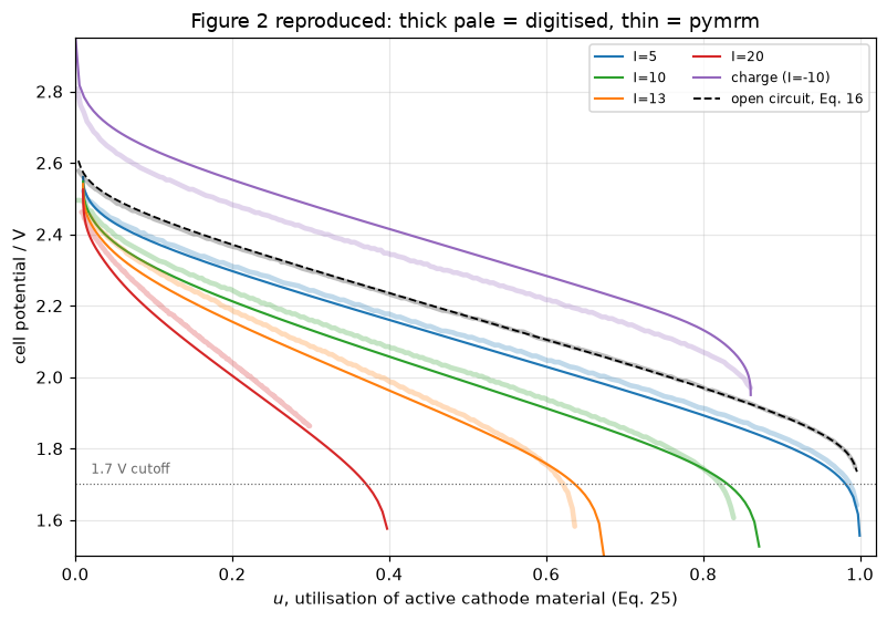
Doyle, M.; Fuller, T. F.; Newman, J. (1993) — Journal of the Electrochemical Society 140(6) 1526-1533 — doi:10.1149/1.2221597 — digitised from Figure 2, journal page 1529display(Markdown(
f"**What the numbers say.** The model is slightly too polarised, everywhere, by an "
f"amount that barely changes with utilisation: the pooled bias is "
f"{CM['discharge_pooled_bias_mV']:.1f} mV against a mean absolute deviation of "
f"{CM['discharge_pooled_mad_mV']:.1f} mV, so almost all of the deviation *is* the bias. "
f"Seen from the other side, every transport-limited crossing of 1.9 V arrives early, "
f"by {100 * CM['u19_shortfall_min']:.1f} to {100 * CM['u19_shortfall_max']:.1f} percentage "
f"points of utilisation. Those are the same defect twice.\n\n"
f"The charge curve says what it is. Reverse the current and the model is "
f"over-polarised by {CM['charge_bias_mV']:.1f} mV in the *opposite* direction: the "
f"deviation follows the sign of $I$, which is the signature of a series resistance "
f"rather than of the kinetics, the open-circuit potential or the diffusivity. That "
f"points at $\\kappa$, the one input that had to be reconstructed, and whose two "
f"routes differ by {KAP['kappa_route_spread_pct']:.0f} %.\n\n"
f"What the page cannot do is carry the *concentration dependence* of $\\kappa$. The "
f"paper is explicit that it matters, and by the end of a discharge much of the "
f"cathode electrolyte is far from its initial concentration. A constant is a "
f"stand-in, and it is the most likely reason the remaining deviation does not "
f"shrink to the digitisation error; that is not measured here, because the "
f"polynomial is not in the paper."))What the numbers say. The model is slightly too polarised, everywhere, by an amount that barely changes with utilisation: the pooled bias is -23.8 mV against a mean absolute deviation of 25.5 mV, so almost all of the deviation is the bias. Seen from the other side, every transport-limited crossing of 1.9 V arrives early, by 1.4 to 3.1 percentage points of utilisation. Those are the same defect twice.
The charge curve says what it is. Reverse the current and the model is over-polarised by 64.9 mV in the opposite direction: the deviation follows the sign of \(I\), which is the signature of a series resistance rather than of the kinetics, the open-circuit potential or the diffusivity. That points at \(\kappa\), the one input that had to be reconstructed, and whose two routes differ by 19 %.
What the page cannot do is carry the concentration dependence of \(\kappa\). The paper is explicit that it matters, and by the end of a discharge much of the cathode electrolyte is far from its initial concentration. A constant is a stand-in, and it is the most likely reason the remaining deviation does not shrink to the digitisation error; that is not measured here, because the polynomial is not in the paper.
The porosity optimisation the paper reports as one sentence
At \(I=10\) A/m², holding the theoretical capacity fixed by thickening the cathode as it is made more porous, the paper states that utilisation at the 1.7 V cutoff has a maximum, and gives the porosity and the utilisation there and at the base porosity (the stated-results table). The page scans the whole window the paper discusses, 0.30 to 0.75, then refines the maximum with a bounded maximisation between the scan points either side of the largest value. Each evaluation is one march to 1.6 V and one root of its trace at 1.7 V.
CAPACITY = (1 - P["epsilon"]) * P["delta_c"]          # theoretical capacity per area / (c_T)
POR = np.round(np.arange(0.30, 0.7501, 0.05), 2)


def u_cut(e, P=P, kappa=KAPPA, refine=1, **kw):
    """Utilisation at the 1.7 V cutoff at porosity e and constant theoretical capacity."""
    r = run(10.0, P, kappa, eps=e, delta_c=CAPACITY / (1 - e), v_stop=1.60, refine=refine, **kw)
    return safe_crossing(r["u"], r["V"], P["V_cutoff"])


def porosity_metrics(P=P, kappa=KAPPA, refine=1, distances=(0.05, 0.10, 0.15), **kw):
    scan = np.array([u_cut(e, P, kappa, refine, **kw) for e in POR])
    if not np.all(np.isfinite(scan)):
        return {"porosity_optimum": np.nan, "u_at_optimum": np.nan, "_scan": scan}
    i = int(np.argmax(scan))
    if i in (0, len(POR) - 1):          # a maximum on the window edge is "at or beyond"
        return {"porosity_optimum": np.nan, "u_at_optimum": np.nan, "_scan": scan}
    res = minimize_scalar(lambda e: -u_cut(e, P, kappa, refine, **kw), bounds=(POR[i - 1], POR[i + 1]),
                          method="bounded", options={"xatol": 1e-4})
    e_opt, u_opt = float(res.x), float(-res.fun)
    out = {"porosity_optimum": e_opt, "u_at_optimum": u_opt, "_scan": scan, "_nfev": res.nfev}
    for d in distances:
        out[f"loss_below_{round(100 * d):03d}"] = u_opt - u_cut(e_opt - d, P, kappa, refine, **kw)
        out[f"loss_above_{round(100 * d):03d}"] = u_opt - u_cut(e_opt + d, P, kappa, refine, **kw)
    out["_gap"] = np.array([out[f"loss_above_{round(100 * d):03d}"] - out[f"loss_below_{round(100 * d):03d}"]
                            for d in distances])
    return out


OPT = porosity_metrics()
OPT_COND = "porosity maximising utilisation at I = 10 A/m2 and constant theoretical capacity"
OPT_CUT = "I = 10 A/m2 porosity 0.60 at constant theoretical capacity cutoff 1.7 V"
print(f"{'porosity':>10}{'delta_c/um':>13}{'u at 1.7 V':>13}")
for e, u in zip(POR, OPT["_scan"]):
    print(f"{e:>10.2f}{CAPACITY / (1 - e) * 1e6:>13.1f}{u:>13.4f}")
print(f"\nbounded maximisation between {POR[np.argmax(OPT['_scan']) - 1]:.2f} and "
      f"{POR[np.argmax(OPT['_scan']) + 1]:.2f} ({OPT['_nfev']} marches): optimum at porosity "
      f"{OPT['porosity_optimum']:.4f}, utilisation {OPT['u_at_optimum']:.4f}")
print(f"paper: optimum at porosity {tgt[('porosity_optimum', OPT_COND)]:.2f}, utilisation "
      f"{tgt[('u_at_cutoff', OPT_CUT)]:.2f}")
print(f"\nloss of utilisation at equal distance from the optimum:")
print(f"{'distance':>10}{'below':>10}{'above':>10}")
for d in (0.05, 0.10, 0.15):
    print(f"{d:>10.2f}{OPT[f'loss_below_{round(100 * d):03d}']:>10.4f}"
          f"{OPT[f'loss_above_{round(100 * d):03d}']:>10.4f}")
claims.value("porosity_optimum", OPT["porosity_optimum"], rtol=0.01)
claims.value("u_at_optimum", OPT["u_at_optimum"])
for d in (0.05, 0.10, 0.15):
    for side in ("below", "above"):
        claims.value(f"loss_{side}_{round(100 * d):03d}", OPT[f"loss_{side}_{round(100 * d):03d}"])
N_ABOVE = claims.count("loss_above_exceeds_below_count", OPT["_gap"], 0.0, min_margin=5e-5,
                       note="distances 0.05, 0.10, 0.15 at which the loss above the optimum is the "
                            "larger; margin = smallest difference of the two losses")

fig, ax = plt.subplots(figsize=(6.4, 4.0))
ax.plot(POR, 100 * OPT["_scan"], "o-", color="tab:green", lw=1.6, ms=5, label="pymrm, scan")
ax.plot([OPT["porosity_optimum"]], [100 * OPT["u_at_optimum"]], "s", color="tab:green", ms=7,
        mfc="white", label="pymrm, refined maximum")
ax.plot([0.30, tgt[("porosity_optimum", OPT_COND)]],
        [100 * tgt[("u_at_cutoff", "I = 10 A/m2 porosity 0.30 separator 50 um cutoff 1.7 V")],
         100 * tgt[("u_at_cutoff", OPT_CUT)]], "k*", ms=13, label="stated in the paper")
ax.set(xlabel="cathode porosity (thickness adjusted at constant capacity)",
       ylabel="utilisation at the 1.7 V cutoff / %",
       title="the optimisation the paper reports as one number, swept")
ax.legend(fontsize=8)
fig.tight_layout()
plt.show()
porosity delta_c/um u at 1.7 V
0.30 100.0 0.8312
0.35 107.7 0.8741
0.40 116.7 0.8994
0.45 127.3 0.9141
0.50 140.0 0.9227
0.55 155.6 0.9271
0.60 175.0 0.9282
0.65 200.0 0.9257
0.70 233.3 0.9184
0.75 280.0 0.9029
bounded maximisation between 0.55 and 0.65 (7 marches): optimum at porosity 0.5907, utilisation 0.9282
paper: optimum at porosity 0.60, utilisation 0.97
loss of utilisation at equal distance from the optimum:
distance below above
0.05 0.0016 0.0018
0.10 0.0068 0.0080
0.15 0.0163 0.0216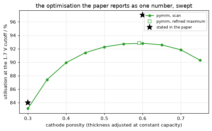
display(Markdown(
    f"The model's optimum is at a porosity of {OPT['porosity_optimum']:.3f}, "
    f"{abs(OPT['porosity_optimum'] - tgt[('porosity_optimum', OPT_COND)]):.3f} below the "
    f"paper's {tgt[('porosity_optimum', OPT_COND)]:.2f}; the scan's largest value is at the "
    f"{POR[np.argmax(OPT['_scan'])]:.2f} node, and the maximum is flat: the utilisation there "
    f"is {OPT['u_at_optimum']:.3f}, against the paper's {tgt[('u_at_cutoff', OPT_CUT)]:.2f}. "
    f"The curve is not steeper below the optimum than above it: at equal distances the loss "
    f"above is the larger at {N_ABOVE} of the three distances tabulated, "
    f"{OPT['loss_above_015']:.4f} against {OPT['loss_below_015']:.4f} at 0.15. It only looks "
    f"steeper below because the window reaches further below the optimum than above it."))
The model’s optimum is at a porosity of 0.591, 0.009 below the paper’s 0.60; the scan’s largest value is at the 0.60 node, and the maximum is flat: the utilisation there is 0.928, against the paper’s 0.97. The curve is not steeper below the optimum than above it: at equal distances the loss above is the larger at 3 of the three distances tabulated, 0.0216 against 0.0163 at 0.15. It only looks steeper below because the window reaches further below the optimum than above it.
Validation
Each check says what it can catch, and the break table at the end measures it.
- Identities of the scheme: the utilisation against Faraday’s law, total salt, and the mean pore-wall flux. Each is exact by construction for the interior physics and tests one specific coupling or boundary condition.
- The short-time concentration rise at the anode, against the semi-infinite analytical solution, with no conductivity in it and nothing fitted.
- Refinement in space and in time, each on its own ladder with the other axis held fixed.
- The Bruggeman exponent in the salt flux and the factor in Eq. 5, which the paper leaves ambiguous, confronted with its own results.
- The utilisation the paper states at the 1.7 V cutoff.
1. Identities of the scheme
Faraday’s law. Summing the solid balance over the cathode and using the charge balance, \(\frac{d}{dt}\sum(1-\epsilon)\Delta x\,c_s = -\sum a i\,\Delta x/F = I/F\), so the utilisation computed from the state must equal \(u_0 + It/\big(F(1-\epsilon)c_T\delta_c\big)\) at every step. It fails when the pore-wall current enters the solid and charge balances differently.
Salt. \(\sum_i\Delta x_i(\nabla\cdot\mathbf{N})_i = N_{\rm end}-N_0\) for any interior flux, so \(\sum\epsilon\Delta x\,c\) is constant whatever the migration term, the transference number or the reaction coupling, and changes only when a boundary flux is wrong. The drift under the three interior defects of the break table is registered as structural: no interior defect can move it.
Mean pore-wall flux. Summing the charge balance gives \(\sum a i\,\Delta x = -I\), so the mean flux \(j_n\) over the cathode is \(-I/(F a\delta_c)\) at any time, for any distribution. It fails when the current in the charge balance is not the one reported.
def identity_metrics(r):
    """The three identities on one I = 10 march."""
    c = r["cell"]
    u_faraday = P["u_0"] + 10.0 * r["t"] / c.t_full
    return {"faraday_gap": float(np.max(np.abs(r["u"] - u_faraday))),
            "salt_conservation_drift": float(np.max(np.abs(r["salt"] / r["salt"][0] - 1)))}


def wall_flux_gap(P=P, kappa=KAPPA, **kw):
    """Mean pore-wall flux at 7000 s against the charge balance, relative."""
    r = run(10.0, P, kappa, nodes=[7000.0], t_stop=7000.0, **kw)
    jm, jn = r["cell"].wall_flux_mean(r["snaps"][7000.0])
    bal = -10.0 / (F_CONST * r["cell"].a[r["cell"].cathode][0] * r["cell"].dc)
    return abs(jm / bal - 1.0), jm, bal, jn


IDN = identity_metrics(RUNS["I=10"])
WG, JM, JB, JN = wall_flux_gap()
n_steps10 = len(RUNS["I=10"]["t"]) - 1
print(f"I = 10, {n_steps10} steps:")
print(f"  utilisation from the state against Faraday's law: below 1e-12 (here {IDN['faraday_gap']:.1e})")
print(f"  total salt, largest relative drift: below 1e-12 (here {IDN['salt_conservation_drift']:.1e})")
print(f"  mean pore-wall flux at 7000 s against -I/(F a delta_c) = {JB:.4e} mol/(m2 s): "
      f"relative gap below 1e-10 (here {WG:.1e})")
print(f"  the flux itself ranges over {JN.min():.2e} to {JN.max():.2e} mol/(m2 s) across the cathode;")
print("  negative is insertion. The paper's Fig. 5 reads about -0.5e-6 over 2800 to 12600 s.")
claims.bound("faraday_gap", IDN["faraday_gap"], max=1e-12, basis="identity",
             note="state utilisation against u0 + I t / (F (1-eps) c_T delta_c), I = 10 march")
claims.bound("salt_conservation_drift", IDN["salt_conservation_drift"], max=1e-12, basis="identity",
             note="relative drift of sum(eps dx c) over the I = 10 discharge")
claims.bound("wall_flux_identity_gap", WG, max=1e-10, basis="identity",
             note="mean j_n over the cathode at 7000 s against -I/(F a delta_c); newton tolerance")
I = 10, 162 steps:
utilisation from the state against Faraday's law: below 1e-12 (here 3.3e-16)
total salt, largest relative drift: below 1e-12 (here 1.0e-15)
mean pore-wall flux at 7000 s against -I/(F a delta_c) = -4.9353e-07 mol/(m2 s): relative gap below 1e-10 (here 1.2e-12)
the flux itself ranges over -5.63e-07 to -3.16e-07 mol/(m2 s) across the cathode;
negative is insertion. The paper's Fig. 5 reads about -0.5e-6 over 2800 to 12600 s.2. The separator at short times
For the first seconds the separator is semi-infinite, \(\sqrt{Dt}\ll\delta_s\), and the salt rises at the lithium face as \(c(0,t)-c_0 = 2J\sqrt{t/\pi D}\) with \(J = I(1-t^0_+)/F\), for constant \(t^0_+\). No conductivity enters and nothing is fitted. The model’s face value comes from the same boundary condition the residual uses; the value in the first cell centre, half a cell away, is printed beside it. The steps of the short march are refined 16-fold over the production schedule, and a control run with \(t^0_+\) held at its initial value, where the analytical solution is exact apart from the finite separator, shows what is left.
The Fig. 4 column is this page’s reading of the paper’s Figure 4, by eye, to the nearest 5 mol/m³; no CSV holds it.
TIMES = [1.0, 2.0, 5.0, 10.0, 20.0]
FIG4_READ = {1.0: 1020, 2.0: 1045, 5.0: 1075, 10.0: 1100, 20.0: 1150}   # by eye, +-5 mol/m3


def short_time(P=P, kappa=KAPPA, refine=16, n_s=48, n_c=96, **kw):
    """Face and first-cell concentration at TIMES, I = 10, and the semi-infinite solution."""
    r = run(10.0, P, kappa, n_s=n_s, n_c=n_c, nodes=TIMES, t_stop=TIMES[-1], refine=refine, **kw)
    c = r["cell"]
    face = np.array([c.boundary(r["snaps"][t], 10.0)[0] for t in TIMES])
    first = np.array([c.unpack(r["snaps"][t])[0][0] for t in TIMES])
    J = 10.0 * (1 - c.t0_plus(P["c_0"])) / F_CONST
    ana = P["c_0"] + 2 * J * np.sqrt(np.array(TIMES) / (np.pi * P["D"]))
    return face, first, ana


def short_metrics(P=P, kappa=KAPPA, **kw):
    face, first, ana = short_time(P, kappa, **kw)
    fig4 = np.array([FIG4_READ[t] for t in TIMES])
    return {"short_time_face_dev_mean": float(np.mean(np.abs(face - ana))),
            "short_time_face_dev_20s": float(face[-1] - ana[-1]),
            "short_time_first_cell_offset_mean": float(np.mean(face - first)),
            "fig4_dev_max": float(np.max(np.abs(face - fig4))),
            "_face": face, "_first": first, "_ana": ana, "_fig4": fig4}


SH = short_metrics()
SH1 = short_metrics(refine=1)
P_T0 = dict(P, t0_a=P["t0_a"] + P["t0_b"] * P["c_0"], t0_b=0.0)
CTRL = short_metrics(P_T0)
print("concentration at the lithium face, I = 10 A/m2, 48 + 96 cells, steps refined 16-fold")
print(f"{'t/s':>6}{'face':>10}{'1st cell':>10}{'analytic':>10}{'face-ana':>10}"
      f"{'control':>10}{'Fig. 4':>8}")
for k, t in enumerate(TIMES):
    print(f"{t:>6.0f}{SH['_face'][k]:>10.1f}{SH['_first'][k]:>10.1f}{SH['_ana'][k]:>10.1f}"
          f"{SH['_face'][k] - SH['_ana'][k]:>10.2f}{CTRL['_face'][k] - CTRL['_ana'][k]:>10.2f}"
          f"{SH['_fig4'][k]:>8d}")
print(f"\nmean |face - analytic| over the five times: {SH['short_time_face_dev_mean']:.2f} mol/m3"
      f" (production steps: {SH1['short_time_face_dev_mean']:.2f})")
print(f"the first cell centre sits {SH['short_time_first_cell_offset_mean']:.1f} mol/m3 below the face"
      f" on average; read there, the production-step deviation would be "
      f"{np.mean(np.abs(SH1['_first'] - SH1['_ana'])):.1f} mol/m3")
print(f"control with constant t0+: largest |face - analytic| up to 10 s "
      f"{np.max(np.abs(CTRL['_face'] - CTRL['_ana'])[:4]):.2f} mol/m3, at 20 s "
      f"{abs(CTRL['short_time_face_dev_20s']):.2f}")
n_fig4 = claims.count("fig4_beyond_reading_count", np.abs(SH["_face"] - SH["_fig4"]), 5.0,
                      min_margin=0.05, note="times at which the model differs from the Fig. 4 "
                                            "read by more than its 5 mol/m3 resolution")
print(f"model against the Fig. 4 read: largest difference {SH['fig4_dev_max']:.1f} mol/m3, "
      f"beyond the 5 mol/m3 reading at {n_fig4} of {len(TIMES)} times")
for k in ("short_time_face_dev_mean", "short_time_face_dev_20s",
          "short_time_first_cell_offset_mean", "fig4_dev_max"):
    claims.value(k, SH[k], unit="mol/m3")
claims.value("short_time_face_dev_mean_production_steps", SH1["short_time_face_dev_mean"],
             unit="mol/m3")
claims.value("short_time_first_cell_dev_mean_production_steps",
             float(np.mean(np.abs(SH1["_first"] - SH1["_ana"]))), unit="mol/m3")
CTRL_MAX10 = float(np.max(np.abs(CTRL["_face"] - CTRL["_ana"])[:4]))
claims.bound("short_time_control_dev_max_10s", CTRL_MAX10, max=0.2, basis="theory",
             note="constant t0+: the semi-infinite solution is exact up to 10 s apart from the "
                  "first-order step error (about 0.1 mol/m3 at refine 16)")
concentration at the lithium face, I = 10 A/m2, 48 + 96 cells, steps refined 16-fold
t/s face 1st cell analytic face-ana control Fig. 4
1 1035.7 1030.0 1035.9 -0.20 -0.11 1020
2 1050.5 1044.7 1050.8 -0.27 -0.09 1045
5 1079.7 1073.9 1080.2 -0.56 -0.11 1075
10 1112.5 1106.6 1113.5 -1.02 -0.13 1100
20 1158.4 1152.6 1160.5 -2.09 -0.32 1150
mean |face - analytic| over the five times: 0.83 mol/m3 (production steps: 2.60)
the first cell centre sits 5.8 mol/m3 below the face on average; read there, the production-step deviation would be 8.4 mol/m3
control with constant t0+: largest |face - analytic| up to 10 s 0.13 mol/m3, at 20 s 0.32
model against the Fig. 4 read: largest difference 15.7 mol/m3, beyond the 5 mol/m3 reading at 4 of 5 timesdisplay(Markdown(
f"The deviation from the semi-infinite solution grows with time, to "
f"{SH['short_time_face_dev_20s']:.2f} mol/m³ at 20 s, and the control shows why: with "
f"$t^0_+$ held constant the model and the analytical solution agree to within "
f"{CTRL_MAX10:.2f} mol/m³ up to 10 s, the size of the step error. What is left in the "
f"page's own run is the concentration dependence of $t^0_+$, which the analytical "
f"solution leaves out: $(1-t^0_+)$ falls as the salt accumulates at the face. The "
f"first cell centre is {SH['short_time_first_cell_offset_mean']:.1f} mol/m³ below the "
f"face, because the gradient there is steep; reading the cell centre as the face value "
f"would triple the deviation."))The deviation from the semi-infinite solution grows with time, to -2.09 mol/m³ at 20 s, and the control shows why: with \(t^0_+\) held constant the model and the analytical solution agree to within 0.13 mol/m³ up to 10 s, the size of the step error. What is left in the page’s own run is the concentration dependence of \(t^0_+\), which the analytical solution leaves out: \((1-t^0_+)\) falls as the salt accumulates at the face. The first cell centre is 5.8 mol/m³ below the face, because the gradient there is steep; reading the cell centre as the face value would triple the deviation.
3. Refinement in space and in time
The quantity is the cell potential at \(u=0.5\), \(I=10\) A/m², at a time that is a step time at every level. Space: four grids from 12 + 24 to 96 + 192 cells on the production time grid. Time: the production grid with every step split into 1, 2, 4 and 8. Orders come from successive differences (pymrm.checks.observed_orders), and the finest difference must be at least \(10^3\) times the floor set by round-off and the Newton tolerance, \(n_{\rm steps}\,\varepsilon\,V + 10^{-9}RT/F\), or the order would be fitted to noise. The errors of the production settings follow by Richardson extrapolation from the finest triple.
def v_half(n_s=24, n_c=48, refine=1, P=P, kappa=KAPPA, **kw):
    """Cell potential at u = 0.5, I = 10, as a step time of the march."""
    c = Cell(P, kappa, n_s=n_s, n_c=n_c, **{k: kw.pop(k) for k in list(kw) if k == "face_mean"})
    t_half = c.t_full / 10.0 * (0.5 - P["u_0"])
    r = c.march(10.0, nodes=[t_half], t_stop=t_half, refine=refine, **kw)
    if r["halvings"]:
        raise RuntimeError("a ladder step was split, so the levels are not nested")
    return c.cell_potential(r["snaps"][t_half], 10.0), len(r["t"]) - 1


def ladder_metrics(levels_x=(12, 24, 48, 96), levels_t=(1, 2, 4, 8), ratio_t=None, **kw):
    VX = {n: v_half(n, 2 * n, **kw) for n in levels_x}
    VT = {m: v_half(refine=m, **kw) for m in levels_t}
    ox = observed_orders(lambda n: VX[n][0], levels_x)
    ot = observed_orders(lambda m: VT[m][0], levels_t, ratio=ratio_t)
    floor = lambda v, n: n * EPS * abs(v) + 1e-9 * RTF
    fx = abs(VX[levels_x[-1]][0] - VX[levels_x[-2]][0]) / floor(*VX[levels_x[-1]])
    ft = abs(VT[levels_t[-1]][0] - VT[levels_t[-2]][0]) / floor(*VT[levels_t[-1]])
    return {"grid_order_min": min(ox["orders"]), "grid_order_max": max(ox["orders"]),
            "grid_finest_over_roundoff": fx,
            "grid_error_mV": 1e3 * abs(VX[24][0] - ox["extrapolated"]) if 24 in VX else np.nan,
            "dt_order_min": min(ot["orders"]), "dt_order_max": max(ot["orders"]),
            "dt_finest_over_roundoff": ft,
            "dt_spread_mV": 1e3 * abs(VT[levels_t[0]][0] - ot["extrapolated"]),
            "_VX": VX, "_VT": VT, "_ox": ox, "_ot": ot}


LAD = ladder_metrics()
print("space, production time grid       V(u=0.5)/V      steps    order")
for k, n in enumerate((12, 24, 48, 96)):
    o = f"{LAD['_ox']['orders'][k - 2]:8.3f}" if k >= 2 else ""
    print(f"   {n:4d} + {2 * n:4d} cells          {LAD['_VX'][n][0]:.9f}   {LAD['_VX'][n][1]:6d}  {o}")
print("time, 24 + 48 cells")
for k, m in enumerate((1, 2, 4, 8)):
    o = f"{LAD['_ot']['orders'][k - 2]:8.3f}" if k >= 2 else ""
    print(f"   steps split into {m}            {LAD['_VT'][m][0]:.9f}   {LAD['_VT'][m][1]:6d}  {o}")
print(f"\nspatial order {LAD['grid_order_min']:.3f} to {LAD['grid_order_max']:.3f}; error of the "
      f"production grid {LAD['grid_error_mV']:.3f} mV")
print(f"temporal order {LAD['dt_order_min']:.3f} to {LAD['dt_order_max']:.3f}; error of the "
      f"production steps {LAD['dt_spread_mV']:.3f} mV")
print(f"finest difference over its floor: space above 1e3 (here {LAD['grid_finest_over_roundoff']:.1e}),"
      f" time above 1e3 (here {LAD['dt_finest_over_roundoff']:.1e})")
claims.bound("grid_order_min", LAD["grid_order_min"], min=1.8, max=2.2, basis="theory",
             note="cell-centred scheme, harmonic face means at the porosity jump: order 2")
claims.bound("grid_order_max", LAD["grid_order_max"], min=1.8, max=2.2, basis="theory",
             note="as grid_order_min")
claims.bound("dt_order_min", LAD["dt_order_min"], min=0.9, max=1.1, basis="theory",
             note="backward Euler on a nested time grid: order 1")
claims.bound("dt_order_max", LAD["dt_order_max"], min=0.9, max=1.1, basis="theory",
             note="as dt_order_min")
claims.bound("grid_finest_over_roundoff", LAD["grid_finest_over_roundoff"], min=1e3, basis="theory",
             note="finest spatial difference over n_steps eps V + 1e-9 RT/F")
claims.bound("dt_finest_over_roundoff", LAD["dt_finest_over_roundoff"], min=1e3, basis="theory",
             note="finest temporal difference over n_steps eps V + 1e-9 RT/F")
claims.value("grid_error_mV", LAD["grid_error_mV"], unit="mV")
claims.value("dt_spread_mV", LAD["dt_spread_mV"], unit="mV")
space, production time grid V(u=0.5)/V steps order
12 + 24 cells 1.984934490 101
24 + 48 cells 1.985018395 101
48 + 96 cells 1.985039350 101 2.001
96 + 192 cells 1.985044586 101 2.001
time, 24 + 48 cells
steps split into 1 1.985018395 101
steps split into 2 1.984881299 202
steps split into 4 1.984812904 404 1.003
steps split into 8 1.984778748 808 1.002
spatial order 2.001 to 2.001; error of the production grid 0.028 mV
temporal order 1.002 to 1.003; error of the production steps 0.274 mV
finest difference over its floor: space above 1e3 (here 1.6e+05), time above 1e3 (here 1.1e+06)The headline is a mean over every digitised point, not one potential, and its early points sit where the steps are still growing, so it is checked directly too: the five curves recomputed with every step split into 2 and into 4, and on the 48 + 96 grid.
def order_and_limit(q, ratio):
    """Order and Richardson limit from three successive values read with ``ratio``."""
    order = np.log(abs(q[0] - q[1]) / abs(q[1] - q[2])) / np.log(ratio)
    return order, q[2] + (q[2] - q[1]) / (ratio ** order - 1)


def headline_metrics(levels=(1, 2, 4), ratio=None, n_s=24, n_c=48, base=None, sets=None,
                     limit="extrapolated"):
    if sets is None:
        sets = {m: (base if (m == 1 and base is not None) else
                    curve_metrics(discharge_runs(charge=True, n_s=n_s, n_c=n_c, refine=m)))
                for m in levels}
    out = {}
    for key, tag in (("discharge_pooled_mad_mV", "pooled"), ("mad_I20_mV", "I20")):
        q = [sets[m][key] for m in levels]
        if ratio is None:
            o = observed_orders(lambda m: sets[m][key], levels)
            order, ext = o["orders"][-1], o["extrapolated"]
        else:                       # a ladder read with an assumed ratio (break rows)
            order, ext = order_and_limit(q[-3:], ratio)
        out[f"headline_dt_order_{tag}"] = order
        if limit == "finest":       # the finest level taken as the limit (break rows)
            ext = q[-1]
        out[f"headline_dt_error_{tag}_mV"] = ext - q[0]     # how far below its limit
        out[f"_ext_{tag}"] = ext
    out["_sets"] = sets
    return out


def grid_change(n_s=24, n_c=48, base=None):
    coarse = base if base is not None else curve_metrics(discharge_runs(charge=True, n_s=n_s, n_c=n_c))
    fine = curve_metrics(discharge_runs(charge=True, n_s=2 * n_s, n_c=2 * n_c))
    keys = ("discharge_pooled_mad_mV", "mad_charge_mV")
    return max(abs(fine[k] - coarse[k]) for k in keys)


HL = headline_metrics(base=CM)
HC_GRID = grid_change(base=CM)
print(f"{'steps split into':>18}{'pooled MAD':>12}{'I=20 MAD':>10}{'charge MAD':>12}  (mV)")
for m, cmm in HL["_sets"].items():
    print(f"{m:>18d}{cmm['discharge_pooled_mad_mV']:>12.3f}{cmm['mad_I20_mV']:>10.3f}"
          f"{cmm['mad_charge_mV']:>12.3f}")
print(f"{'extrapolated':>18}{HL['_ext_pooled']:>12.3f}{HL['_ext_I20']:>10.3f}")
print(f"\nobserved order in the step: pooled {HL['headline_dt_order_pooled']:.3f}, "
      f"I = 20 {HL['headline_dt_order_I20']:.3f}")
print(f"the production steps leave the pooled MAD {HL['headline_dt_error_pooled_mV']:.2f} mV and "
      f"the I = 20 MAD {HL['headline_dt_error_I20_mV']:.2f} mV below their zero-step limits")
print(f"grid doubled: pooled and charge MAD move by below 0.05 mV (here {HC_GRID:.3f})")
for tag in ("pooled", "I20"):
    claims.bound(f"headline_dt_order_{tag}", HL[f"headline_dt_order_{tag}"], min=0.8, max=1.2,
                 basis="theory", note="steps split into 1, 2, 4: backward Euler, order 1")
    claims.value(f"headline_dt_error_{tag}_mV", HL[f"headline_dt_error_{tag}_mV"], unit="mV")
claims.bound("headline_change_grid_mV", HC_GRID, max=0.05, basis="chosen",
             note="pooled and charge MAD, 24+48 against 48+96 cells; half the 0.1 mV printed "
                  "resolution")
steps split into pooled MAD I=20 MAD charge MAD (mV)
1 25.522 33.958 65.101
2 25.924 34.896 65.090
4 26.124 35.366 65.146
extrapolated 26.323 35.838
observed order in the step: pooled 1.004, I = 20 0.996
the production steps leave the pooled MAD 0.80 mV and the I = 20 MAD 1.88 mV below their zero-step limits
grid doubled: pooled and charge MAD move by below 0.05 mV (here 0.043)display(Markdown(
f"The step, not the grid, is the numerical error of the headline: the production steps "
f"leave the pooled deviation {abs(HL['headline_dt_error_pooled_mV']):.1f} mV below its "
f"zero-step limit, and the largest step error is at $I$ = 20 A/m², "
f"{abs(HL['headline_dt_error_I20_mV']):.1f} mV. Both are small against the "
f"model-figure deviation itself, so no conclusion below moves; the numbers are quoted "
f"at the production steps."))The step, not the grid, is the numerical error of the headline: the production steps leave the pooled deviation 0.8 mV below its zero-step limit, and the largest step error is at \(I\) = 20 A/m², 1.9 mV. Both are small against the model-figure deviation itself, so no conclusion below moves; the numbers are quoted at the production steps.
4. The Bruggeman exponent the paper leaves ambiguous
Table I writes the cathode salt equation with the flux as \(\nabla\cdot(\epsilon D\nabla c)\), and the text separately defines \(D_{\rm eff}=D\epsilon^{0.5}\). Read together they give a flux coefficient \(D\epsilon^{1.5}\); read as the text defining the coefficient Table I calls \(\epsilon D\), they give \(D\epsilon^{0.5}\). The two differ by a factor \(1/\epsilon\) and the paper does not say which it used.
Its own results settle it. The table runs all three readings at the same recovered conductivity and compares the 1.9 V crossing, which is transport-limited and set nothing. The paper’s Figure 3 has the electrolyte still positive at 12 600 s at \(I=10\) A/m²; the last column is the utilisation at which the salt concentration first falls below 1 mol/m³ somewhere in the cell.
U19_PUB = np.array([FIG_X[k][1.9] for k in CURVES])


def sweep(P=P, kappa=KAPPA, **kw):
    runs = discharge_runs(P, kappa, **kw)
    m = curve_metrics(runs)
    u19 = np.array([safe_crossing(runs[k]["u"], runs[k]["V"], 1.9) for k in CURVES])
    r10 = runs["I=10"]
    dead = r10["u"][np.argmax(r10["c_min"] < 1.0)] if np.any(r10["c_min"] < 1.0) else np.nan
    return {"u19": u19, "mean_du": float(np.mean(np.abs(u19 - U19_PUB))),
            "bias": float(np.mean(u19 - U19_PUB)), "mad": m["discharge_pooled_mad_mV"],
            "ratio_min": float(np.min(u19 / U19_PUB)), "ratio_max": float(np.max(u19 / U19_PUB)),
            "u_salt_out_I10": float(dead), "ends": [runs[k]["end"] for k in CURVES],
            "c_end": [runs[k]["c_min"][-1] for k in CURVES]}


def show(label, s):
    print(f"{label:>16}" + "".join(f"{x:>9.3f}" for x in s["u19"])
          + f"{s['mean_du']:>11.3f}{s['mad']:>9.1f}{s['u_salt_out_I10']:>13.3f}")


def bruggeman_metrics(P=P, kappa=KAPPA, base=None):
    out = {p: sweep(P, kappa, p_D=p) for p in (1.5, 0.0)}
    out[0.5] = sweep(P, kappa) if base is None else base
    return out


BASE_SWEEP = sweep()
BRUG = bruggeman_metrics(base=BASE_SWEEP)
print(f"{'salt flux coeff':>16}" + "".join(f"{k:>9}" for k in CURVES)
      + f"{'mean |du|':>11}{'MAD/mV':>9}{'u, c < 1 (I=10)':>16}")
for p, label in ((1.5, "D eps^1.5"), (0.5, "D eps^0.5"), (0.0, "D")):
    show(label, BRUG[p])
print(f"{'published':>16}" + "".join(f"{x:>9.3f}" for x in U19_PUB))
ends_newton = [c for p in BRUG for e, c in zip(BRUG[p]["ends"], BRUG[p]["c_end"]) if e == "newton"]
print(f"\nmarches that end on a failed solve: {len(ends_newton)}, each with the salt exhausted "
      f"somewhere (smallest c at the last converged step below 0.01 mol/m3)")
print(f"D eps^1.5 reaches 1.9 V at {BRUG[1.5]['ratio_min']:.2f} to {BRUG[1.5]['ratio_max']:.2f} "
      f"of the published utilisation, and exhausts the electrolyte at u = "
      f"{BRUG[1.5]['u_salt_out_I10']:.3f} at I = 10 A/m2.")
D0 = BRUG[0.0]["u19"] - U19_PUB
print("Dropping the porosity correction moves the crossing by "
      + ", ".join(f"{d:+.3f}" for d in D0) + " at I = 5, 10, 13, 20.")
for p, tag in ((1.5, "eps15"), (0.0, "eps0")):
    claims.value(f"brug_mean_du_{tag}", BRUG[p]["mean_du"])
    claims.value(f"brug_mad_{tag}_mV", BRUG[p]["mad"], unit="mV")
claims.value("brug_eps15_ratio_min", BRUG[1.5]["ratio_min"])
claims.value("brug_eps15_ratio_max", BRUG[1.5]["ratio_max"])
claims.value("brug_eps15_u_salt_out_I10", BRUG[1.5]["u_salt_out_I10"])
claims.count("brug_newton_ends_salt_exhausted", -np.log10(np.maximum(ends_newton, 1e-300)), 2.0,
             min_margin=0.05, relative=False,
             note="marches of the three readings that end on a failed solve, with c_min at the "
                  "last converged step below 1e-2 mol/m3; margin in decades")
salt flux coeff I=5 I=10 I=13 I=20 mean |du| MAD/mV u, c < 1 (I=10)
D eps^1.5 0.506 0.250 0.186 0.111 0.294 189.7 0.193
D eps^0.5 0.790 0.617 0.466 0.264 0.023 25.5 0.859
D 0.807 0.710 0.637 0.403 0.086 37.5 nan
published 0.816 0.648 0.486 0.278
marches that end on a failed solve: 5, each with the salt exhausted somewhere (smallest c at the last converged step below 0.01 mol/m3)
D eps^1.5 reaches 1.9 V at 0.38 to 0.62 of the published utilisation, and exhausts the electrolyte at u = 0.193 at I = 10 A/m2.
Dropping the porosity correction moves the crossing by -0.009, +0.062, +0.150, +0.125 at I = 5, 10, 13, 20.54b. The factor the printed Eq. 5 is missing
Eq. 5 as printed gives \(-\frac{RT}{F}(1-t^0_+)\) for the coefficient of \(\nabla\ln c\); a 1:1 salt requires twice that, as argued under Parameters. Figure 2 does not decide this one, and the page says so: the printed version gives a smaller mean deviation but overshoots every transport-limited crossing, while the corrected version undershoots them. What decides it is the thermodynamic identity, not the fit.
NU1 = sweep(nu_factor=1.0)
print(f"{'nu factor':>16}" + "".join(f"{k:>9}" for k in CURVES)
      + f"{'mean |du|':>11}{'MAD/mV':>9}")
for label, s in (("2 (used here)", BASE_SWEEP), ("1 (as printed)", NU1)):
    print(f"{label:>16}" + "".join(f"{x:>9.3f}" for x in s["u19"])
          + f"{s['mean_du']:>11.3f}{s['mad']:>9.1f}")
print(f"{'published':>16}" + "".join(f"{x:>9.3f}" for x in U19_PUB))
print(f"\nsigned mean shift of the 1.9 V crossing: nu = 2 {BASE_SWEEP['bias']:+.3f}, "
      f"nu = 1 {NU1['bias']:+.3f}")
N_BRACKET = claims.count("nu_bracket_count", (NU1["u19"] - U19_PUB) * (U19_PUB - BASE_SWEEP["u19"]),
                         0.0, min_margin=1e-5, relative=False,
                         note="currents at which the two readings of Eq. 5 put the 1.9 V crossing "
                              "on opposite sides of the figure's; margin = smallest product of "
                              "the two distances")
print(f"the two readings bracket the published crossing at {N_BRACKET} of {len(CURVES)} currents")
claims.value("nu1_mad_mV", NU1["mad"], unit="mV")
claims.value("nu1_u19_bias", NU1["bias"])
nu factor I=5 I=10 I=13 I=20 mean |du| MAD/mV
2 (used here) 0.790 0.617 0.466 0.264 0.023 25.5
1 (as printed) 0.817 0.691 0.525 0.301 0.026 18.2
published 0.816 0.648 0.486 0.278
signed mean shift of the 1.9 V crossing: nu = 2 -0.023, nu = 1 +0.026
the two readings bracket the published crossing at 4 of 4 currents5. The utilisation the paper states
Two statements from the paper’s running text, neither of which set anything: the utilisation at which the cell reaches its 1.7 V cutoff at \(I=10\) A/m² and the base porosity (stated-results table), and at \(I=20\) A/m² that the potential “drops sharply when about 30 % of the cathode material is utilized”.
U84_TXT = tgt[("u_at_cutoff", "I = 10 A/m2 porosity 0.30 separator 50 um cutoff 1.7 V")]
u84, u84_fig = CM["u_at_cutoff_I10"], FIG_X["I=10"][1.7]
print("u at the 1.7 V cutoff, I = 10 A/m2, porosity 0.30")
print(f"   pymrm                 {u84:.3f}")
print(f"   digitised Figure 2    {u84_fig:.3f}")
print(f"   stated in the text    {U84_TXT:.2f}")
BETWEEN = bool(min(u84_fig, U84_TXT) < u84 < max(u84_fig, U84_TXT))
claims.exact("u_cutoff_between_figure_and_text", BETWEEN,
             margin=float(min(abs(u84 - u84_fig), abs(u84 - U84_TXT))), min_margin=1e-3,
             note="model between the digitised crossing and the stated 0.84; margin to the "
                  "nearer end")
print(f"   the model sits between the two: {BETWEEN}, {100 * abs(u84 - U84_TXT) / U84_TXT:.1f} % "
      f"from the stated value")
claims.value("u_cutoff_rel_to_stated_pct", 100 * abs(u84 - U84_TXT) / U84_TXT)
print()
print(f"I = 20 A/m2: the published curve is drawn only to u = "
      f"{fig2[fig2.curve == 'I=20'].utilisation.max():.3f}, which the text describes as")
print("   'drops sharply when about 30 % of the cathode material is utilized'.")
print(f"   The model's 1.9 V crossing there is {CM['u19_I20']:.3f} against "
      f"{FIG_X['I=20'][1.9]:.3f} digitised.")
u at the 1.7 V cutoff, I = 10 A/m2, porosity 0.30
pymrm 0.831
digitised Figure 2 0.821
stated in the text 0.84
the model sits between the two: True, 1.1 % from the stated value
I = 20 A/m2: the published curve is drawn only to u = 0.299, which the text describes as
'drops sharply when about 30 % of the cathode material is utilized'.
The model's 1.9 V crossing there is 0.264 against 0.278 digitised.The break table
Each row injects one defect through an argument of Cell or a parameter override, and the claims it can reach are recomputed with it. Transcription defects in the parameter and stated-results tables: a digit changed in \(\zeta\), \(D_s\), \(D\), \(\delta\), \(\nu\), \(k_2\) and \(\sigma\), wherever each enters. Formula defects in the model: the migration sign in the salt flux, \(t^0_+\) written where \((1-t^0_+)\) belongs, the pore-wall current scaled in the charge balance or in the solid balance only, a zero concentration gradient instead of zero salt flux at the lithium, and the arithmetic face mean at the porosity jump. Study defects: ladders read with the wrong refinement ratio, a finest rung that repeats the one before, a doubled step ceiling, a coarse production grid, the control run with \(t^0_+\) varying, and the digitised abscissa read 2 % short. The row for Eq. 5 as printed is a reading, not a defect: it shows which claims depend on the factor.
def kappa_for(P, delta=DELTA):
    return kappa_from_delta(delta, P) / P["epsilon"] ** 1.5


def fast_metrics(P=P, delta=DELTA, nu=NU):
    out = dict(ocp_metrics(P)[0])
    out.update(group_metrics(P))
    out.update(kappa_metrics(P, delta, nu))
    return out


def run_row(row, d):
    for k, v in d.items():
        if not k.startswith("_") and k in claims.metrics:
            brk(row, k, v)


def curve_row(P=P, delta=DELTA, charge=False, **kw):
    runs = discharge_runs(P, kappa_for(P, delta), charge=charge, **kw)
    m = curve_metrics(runs)
    m["u19_below_figure_count"] = int(np.sum(-m["_du19"] > 0))
    m.update(identity_metrics(runs["I=10"]))
    lo, hi = sorted((FIG_X["I=10"][1.7], U84_TXT))
    m["u_cutoff_between_figure_and_text"] = bool(lo < m["u_at_cutoff_I10"] < hi)
    m["u_cutoff_rel_to_stated_pct"] = 100 * abs(m["u_at_cutoff_I10"] - U84_TXT) / U84_TXT
    return m, runs


def short_row(P=P, delta=DELTA, **kw):
    m16 = short_metrics(P, kappa_for(P, delta), **kw)
    m1 = short_metrics(P, kappa_for(P, delta), refine=1, **kw)
    m16["fig4_beyond_reading_count"] = int(np.sum(np.abs(m16["_face"] - m16["_fig4"]) > 5.0))
    m16["short_time_face_dev_mean_production_steps"] = m1["short_time_face_dev_mean"]
    m16["short_time_first_cell_dev_mean_production_steps"] = float(np.mean(np.abs(m1["_first"] - m1["_ana"])))
    return m16


def sweep_row(P=P, delta=DELTA, base=None):
    kap = kappa_for(P, delta)
    b = bruggeman_metrics(P, kap, base=base)
    n1 = sweep(P, kap, nu_factor=1.0)
    ends = [c for p in b for e, c in zip(b[p]["ends"], b[p]["c_end"]) if e == "newton"]
    out = {"nu1_mad_mV": n1["mad"], "nu1_u19_bias": n1["bias"],
           "nu_bracket_count": int(np.sum((n1["u19"] - U19_PUB) * (U19_PUB - b[0.5]["u19"]) > 0)),
           "brug_newton_ends_salt_exhausted": int(np.sum(np.array(ends) < 1e-2)),
           "brug_eps15_ratio_min": b[1.5]["ratio_min"], "brug_eps15_ratio_max": b[1.5]["ratio_max"],
           "brug_eps15_u_salt_out_I10": b[1.5]["u_salt_out_I10"]}
    for p, tag in ((1.5, "eps15"), (0.0, "eps0")):
        out[f"brug_mean_du_{tag}"], out[f"brug_mad_{tag}_mV"] = b[p]["mean_du"], b[p]["mad"]
    return out


def sweep_from_runs(runs):
    """BASE_SWEEP's entries from a set of discharge runs already made."""
    u19 = np.array([safe_crossing(runs[k]["u"], runs[k]["V"], 1.9) for k in CURVES])
    r10 = runs["I=10"]
    dead = r10["u"][np.argmax(r10["c_min"] < 1.0)] if np.any(r10["c_min"] < 1.0) else np.nan
    return {"u19": u19, "mean_du": float(np.mean(np.abs(u19 - U19_PUB))),
            "bias": float(np.mean(u19 - U19_PUB)),
            "mad": curve_metrics(runs)["discharge_pooled_mad_mV"],
            "ratio_min": float(np.min(u19 / U19_PUB)), "ratio_max": float(np.max(u19 / U19_PUB)),
            "u_salt_out_I10": float(dead), "ends": [runs[k]["end"] for k in CURVES],
            "c_end": [runs[k]["c_min"][-1] for k in CURVES]}


def P_with(**over):
    return dict(P, **over)


# transcription defects in the parameter table: closed-form claims
for row, Pb in (("zeta 8.10 -> 8.01 (P)", P_with(zeta=8.01)),
                ("D_s 5.0e-13 -> 5.0e-12 (P)", P_with(D_s=5.0e-12)),
                ("k_2 1.0e-10 -> 1.0e-11 (P)", P_with(k_2=1.0e-11)),
                ("sigma 1.0e4 -> 1.0e5 (P)", P_with(sigma=1.0e5))):
    run_row(row, fast_metrics(Pb))
run_row("nu 68 -> 86 (stated results)", fast_metrics(nu=86.0))

# D: closed forms, curves, the separator at short times, and the three readings
row = "D 7.5e-12 -> 5.7e-12 (P)"
P_D = P_with(D=5.7e-12)
run_row(row, fast_metrics(P_D))
m_D, runs_D = curve_row(P_D)
run_row(row, m_D)
run_row(row, short_row(P_D))
run_row(row, sweep_row(P_D, base=sweep_from_runs(runs_D)))
OPT_D = porosity_metrics(P_D, kappa_for(P_D))
run_row(row, OPT_D)
brk(row, "loss_above_exceeds_below_count", int(np.sum(OPT_D["_gap"] > 0)) if "_gap" in OPT_D else -1)

# delta: the conductivity and everything downstream of it
row = "delta 1.95 -> 1.59 (stated results)"
run_row(row, fast_metrics(delta=1.59))
m_dl, _ = curve_row(delta=1.59, charge=True)
run_row(row, m_dl)

# formula defects in the model
DRIFT_NAMED = []
for row, kw in (("migration sign flipped in N (mig_sign)", dict(mig_sign=+1.0)),
                ("(1 - t0+) written as t0+ in i2 and N (t0_form)", dict(t0_form="t0"))):
    m_f, runs_f = curve_row(**kw)
    run_row(row, m_f)
    run_row(row, short_row(**kw))
    DRIFT_NAMED.append(identity_metrics(runs_f["I=10"])["salt_conservation_drift"])
for row, kw in (("pore-wall current x1.1 in the charge balance (ai_charge)", dict(ai_charge=1.1)),
                ("pore-wall current x1.1 in the solid balance (ai_solid)", dict(ai_solid=1.1)),
                ("zero gradient instead of zero salt flux at the lithium (anion_blocking)",
                 dict(anion_blocking=False))):
    idn = identity_metrics(run(10.0, **kw))
    run_row(row, idn)
    if "ai_charge" in kw:
        DRIFT_NAMED.append(idn["salt_conservation_drift"])
        brk(row, "wall_flux_identity_gap", wall_flux_gap(**kw)[0])

# study defects
row = "control run with t0+ varying (t0_b kept)"
brk(row, "short_time_control_dev_max_10s", float(np.max(np.abs(SH["_face"] - SH["_ana"])[:4])))
row = "Eq. 5 as printed, nu_factor = 1 (a reading)"
brk(row, "u19_below_figure_count", int(np.sum(NU1["u19"] - U19_PUB < 0)))
brk(row, "u19_shortfall_mean", NU1["mean_du"])
row = "digitised utilisation read 2 % short (data)"
for name, lvl, key in (("I=20", 1.9, "u19_I20_digitised"), ("I=10", 1.7, "u17_I10_digitised")):
    s_ = fig2[fig2.curve == name].sort_values("utilisation")
    brk(row, key, safe_crossing(0.98 * s_.utilisation.values, s_.cell_potential_V.values, lvl))
row = "arithmetic face mean at the porosity jump (face_mean)"
VXa = {n: v_half(n, 2 * n, face_mean="arithmetic")[0] for n in (12, 24, 48, 96)}
oxa = observed_orders(lambda n: VXa[n], (12, 24, 48, 96))
brk(row, "grid_order_min", min(oxa["orders"]))
brk(row, "grid_order_max", max(oxa["orders"]))
brk(row, "grid_error_mV", 1e3 * abs(VXa[24] - oxa["extrapolated"]))
row = "time ladder 1, 2, 4 read with ratio 3 (levels)"
_o3, _ = order_and_limit([LAD["_VT"][m][0] for m in (1, 2, 4)], 3)
brk(row, "dt_order_min", _o3)
brk(row, "dt_order_max", _o3)
HL3 = headline_metrics(levels=(1, 2, 4), ratio=3, sets=HL["_sets"])
run_row(row, {k: v for k, v in HL3.items() if k.startswith("headline")})
row = "finest time level taken as the zero-step limit (limit)"
HLF = headline_metrics(levels=(1, 2, 4), limit="finest", sets=HL["_sets"])
run_row(row, {k: v for k, v in HLF.items() if k.startswith("headline")})
row = "finest rung repeats the one before (levels)"
brk(row, "grid_finest_over_roundoff", 0.0 / (LAD["_VX"][48][1] * EPS * abs(LAD["_VX"][48][0]) + 1e-9 * RTF))
brk(row, "dt_finest_over_roundoff", 0.0 / (LAD["_VT"][4][1] * EPS * abs(LAD["_VT"][4][0]) + 1e-9 * RTF))
row = "step ceiling 6e-3 -> 1.2e-2 of t_full/I (dt_max)"
VTd = {m: v_half(refine=m, dt_max=1.2e-2)[0] for m in (1, 2, 4)}
otd = observed_orders(lambda m: VTd[m], (1, 2, 4))
brk(row, "dt_spread_mV", 1e3 * abs(VTd[1] - otd["extrapolated"]))
row = "production grid 6 + 12 cells (n_s, n_c)"
brk(row, "headline_change_grid_mV", grid_change(6, 12))

claims.bound("salt_drift_named_defects_max", max(DRIFT_NAMED), max=1e-12, basis="identity",
             structural=True, note="salt drift under the migration-sign, t0+ and charge-coupling "
                                   "defects: sum(dx div N) telescopes, so no interior defect moves it")

# One line per claim: how many rows fail it, and the first of them.
by_claim = {}
for row_, metric, clean_v, broken, caught in BREAK:
    by_claim.setdefault(metric, []).append((row_, broken, caught))
print(f"{'claim':<46} {'clean':>12} {'rows':>4} {'fail':>4}  first failing row (its value)")
for metric, c in claims.metrics.items():
    rows_m = by_claim.get(metric, [])
    fails = [(r, b) for r, b, k in rows_m if k]
    shown = f"(here {c['value']:.1e})" if c["kind"] == "bound" else f"{float(c['value']):.5g}"
    first = (f"{fails[0][0]} ({float(fails[0][1]):.4g})" if fails
             else ("structural" if c.get("structural") else "NONE"))
    print(f"{metric[:46]:<46} {shown:>12} {len(rows_m):4d} {len(fails):4d}  {first}")
_caught = {mt for _, mt, _, _, k in BREAK if k}
_open = sorted(k for k in claims.metrics if k not in _caught and not claims.metrics[k].get("structural"))
print(f"\n{len(BREAK)} rows over {len(claims.metrics)} claims; {len(_caught)} claims are failed by at "
      f"least one row, {sum(bool(c.get('structural')) for c in claims.metrics.values())} structural; "
      f"open: {', '.join(_open) or 'none'}")
for name in ("salt_conservation_drift", "faraday_gap", "wall_flux_identity_gap"):
    fail = [r for r, _b, k in by_claim.get(name, []) if k]
    held = [r for r, _b, k in by_claim.get(name, []) if not k]
    print(f"{name}: failed by {'; '.join(fail) or 'none'}; held under {len(held)} other rows")
/tmp/claude-1000/-home-eajfpeters-Code-pymrm-suite-pymrm-gallery/87e352fb-4054-4878-884f-1f9fd5ae35e7/scratchpad/wt/pages/J3.4-doyle-fuller-newman/model.py:313: RuntimeWarning: invalid value encountered in sqrt
i01 = P["i_0_1"] * np.sqrt((P["c_max"] - c_b) * c_bclaim clean rows fail first failing row (its value)
ocp_eq16_mad_mV 3.2504 7 1 zeta 8.10 -> 8.01 (P) (3.049)
ocp_eq16_max_mV 26.5 7 1 zeta 8.10 -> 8.01 (P) (23.61)
S_c_at_I10 0.00010211 7 1 D_s 5.0e-13 -> 5.0e-12 (P) (1.021e-05)
S_c_at_I20 0.00020422 7 1 D_s 5.0e-13 -> 5.0e-12 (P) (2.042e-05)
S_s_at_I10 0.15316 7 1 D 7.5e-12 -> 5.7e-12 (P) (0.2015)
i0_initial 47.575 7 1 k_2 1.0e-10 -> 1.0e-11 (P) (4.757)
kappa_eff_from_eq28 0.0079744 7 1 delta 1.95 -> 1.59 (stated results) (0.00978)
kappa_eff_from_eq29 0.0067195 7 2 k_2 1.0e-10 -> 1.0e-11 (P) (0.000672)
kappa_route_spread_pct 18.675 7 3 k_2 1.0e-10 -> 1.0e-11 (P) (1087)
kappa_bulk 0.04853 7 1 delta 1.95 -> 1.59 (stated results) (0.05952)
sigma_over_kappa 2.0606e+05 7 2 sigma 1.0e4 -> 1.0e5 (P) (2.061e+06)
sigma_over_kappa_eq29 2.4454e+05 7 3 k_2 1.0e-10 -> 1.0e-11 (P) (2.445e+06)
sigma_over_kappa_if_bulk 1.254e+06 7 2 sigma 1.0e4 -> 1.0e5 (P) (1.254e+07)
u19_below_figure_count 4 5 3 migration sign flipped in N (mig_sign) (0)
mad_I5_mV 16.811 4 4 D 7.5e-12 -> 5.7e-12 (P) (32.84)
mad_I10_mV 24.117 4 4 D 7.5e-12 -> 5.7e-12 (P) (104.1)
mad_I13_mV 25.931 4 4 D 7.5e-12 -> 5.7e-12 (P) (120)
mad_I20_mV 33.958 4 4 D 7.5e-12 -> 5.7e-12 (P) (145)
mad_charge_mV 65.101 1 1 delta 1.95 -> 1.59 (stated results) (55.32)
discharge_pooled_mad_mV 25.522 4 4 D 7.5e-12 -> 5.7e-12 (P) (99.86)
discharge_pooled_bias_mV -23.785 4 4 D 7.5e-12 -> 5.7e-12 (P) (-99.7)
charge_bias_mV 64.906 1 1 delta 1.95 -> 1.59 (stated results) (55.13)
u19_shortfall_mean 0.022683 5 5 D 7.5e-12 -> 5.7e-12 (P) (0.1139)
u19_shortfall_min 0.014412 4 4 D 7.5e-12 -> 5.7e-12 (P) (0.04781)
u19_shortfall_max 0.030914 4 4 D 7.5e-12 -> 5.7e-12 (P) (0.1689)
u_at_cutoff_I10 0.83116 4 3 D 7.5e-12 -> 5.7e-12 (P) (0.6397)
u19_I20 0.26384 4 3 D 7.5e-12 -> 5.7e-12 (P) (0.1808)
u19_I20_digitised 0.27825 1 1 digitised utilisation read 2 % short (data) (0.2727)
u17_I10_digitised 0.82146 1 1 digitised utilisation read 2 % short (data) (0.805)
porosity_optimum 0.59073 1 1 D 7.5e-12 -> 5.7e-12 (P) (0.6241)
u_at_optimum 0.92823 1 1 D 7.5e-12 -> 5.7e-12 (P) (0.8345)
loss_below_005 0.0016327 1 1 D 7.5e-12 -> 5.7e-12 (P) (0.004287)
loss_above_005 0.0017664 1 1 D 7.5e-12 -> 5.7e-12 (P) (0.004323)
loss_below_010 0.0067799 1 1 D 7.5e-12 -> 5.7e-12 (P) (0.01722)
loss_above_010 0.0080206 1 1 D 7.5e-12 -> 5.7e-12 (P) (0.01741)
loss_below_015 0.016293 1 1 D 7.5e-12 -> 5.7e-12 (P) (0.03953)
loss_above_015 0.021567 1 1 D 7.5e-12 -> 5.7e-12 (P) (0.03941)
loss_above_exceeds_below_count 3 1 1 D 7.5e-12 -> 5.7e-12 (P) (2)
faraday_gap (here 3.3e-16) 7 2 pore-wall current x1.1 in the charge balance (ai_charge) (0.08594)
salt_conservation_drift (here 1.0e-15) 7 1 zero gradient instead of zero salt flux at the lithium (anion_blocking) (0.7444)
wall_flux_identity_gap (here 1.2e-12) 1 1 pore-wall current x1.1 in the charge balance (ai_charge) (0.09091)
fig4_beyond_reading_count 4 3 3 D 7.5e-12 -> 5.7e-12 (P) (5)
short_time_face_dev_mean 0.82676 3 3 D 7.5e-12 -> 5.7e-12 (P) (1.03)
short_time_face_dev_20s -2.0925 3 3 D 7.5e-12 -> 5.7e-12 (P) (-2.553)
short_time_first_cell_offset_mean 5.789 3 3 D 7.5e-12 -> 5.7e-12 (P) (7.569)
fig4_dev_max 15.686 3 3 D 7.5e-12 -> 5.7e-12 (P) (31.54)
short_time_face_dev_mean_production_steps 2.5958 3 3 D 7.5e-12 -> 5.7e-12 (P) (3.031)
short_time_first_cell_dev_mean_production_step 8.3686 3 3 D 7.5e-12 -> 5.7e-12 (P) (10.58)
short_time_control_dev_max_10s (here 1.3e-01) 1 1 control run with t0+ varying (t0_b kept) (1.019)
grid_order_min (here 2.0e+00) 1 1 arithmetic face mean at the porosity jump (face_mean) (0.9509)
grid_order_max (here 2.0e+00) 1 1 arithmetic face mean at the porosity jump (face_mean) (0.976)
dt_order_min (here 1.0e+00) 1 1 time ladder 1, 2, 4 read with ratio 3 (levels) (0.633)
dt_order_max (here 1.0e+00) 1 1 time ladder 1, 2, 4 read with ratio 3 (levels) (0.633)
grid_finest_over_roundoff (here 1.6e+05) 1 1 finest rung repeats the one before (levels) (0)
dt_finest_over_roundoff (here 1.1e+06) 1 1 finest rung repeats the one before (levels) (0)
grid_error_mV 0.027935 1 1 arithmetic face mean at the porosity jump (face_mean) (1.359)
dt_spread_mV 0.27372 1 1 step ceiling 6e-3 -> 1.2e-2 of t_full/I (dt_max) (0.52)
headline_dt_order_pooled (here 1.0e+00) 2 1 time ladder 1, 2, 4 read with ratio 3 (levels) (0.6333)
headline_dt_error_pooled_mV 0.80114 2 1 finest time level taken as the zero-step limit (limit) (0.6019)
headline_dt_order_I20 (here 1.0e+00) 2 1 time ladder 1, 2, 4 read with ratio 3 (levels) (0.6285)
headline_dt_error_I20_mV 1.8803 2 1 finest time level taken as the zero-step limit (limit) (1.408)
headline_change_grid_mV (here 4.3e-02) 1 1 production grid 6 + 12 cells (n_s, n_c) (0.6888)
brug_mean_du_eps15 0.29395 1 1 D 7.5e-12 -> 5.7e-12 (P) (0.3568)
brug_mad_eps15_mV 189.7 1 1 D 7.5e-12 -> 5.7e-12 (P) (217.9)
brug_mean_du_eps0 0.086323 1 1 D 7.5e-12 -> 5.7e-12 (P) (0.02145)
brug_mad_eps0_mV 37.511 1 1 D 7.5e-12 -> 5.7e-12 (P) (23.64)
brug_eps15_ratio_min 0.3826 1 1 D 7.5e-12 -> 5.7e-12 (P) (0.2846)
brug_eps15_ratio_max 0.61984 1 1 D 7.5e-12 -> 5.7e-12 (P) (0.4817)
brug_eps15_u_salt_out_I10 0.19335 1 1 D 7.5e-12 -> 5.7e-12 (P) (0.1453)
brug_newton_ends_salt_exhausted 5 1 1 D 7.5e-12 -> 5.7e-12 (P) (4)
nu_bracket_count 4 1 1 D 7.5e-12 -> 5.7e-12 (P) (0)
nu1_mad_mV 18.195 1 1 D 7.5e-12 -> 5.7e-12 (P) (55.45)
nu1_u19_bias 0.026421 1 1 D 7.5e-12 -> 5.7e-12 (P) (-0.07203)
u_cutoff_between_figure_and_text 1 4 3 D 7.5e-12 -> 5.7e-12 (P) (0)
u_cutoff_rel_to_stated_pct 1.0522 4 4 D 7.5e-12 -> 5.7e-12 (P) (23.85)
salt_drift_named_defects_max (here 3.2e-14) 0 0 structural
227 rows over 76 claims; 75 claims are failed by at least one row, 1 structural; open: none
salt_conservation_drift: failed by zero gradient instead of zero salt flux at the lithium (anion_blocking); held under 6 other rows
faraday_gap: failed by pore-wall current x1.1 in the charge balance (ai_charge); pore-wall current x1.1 in the solid balance (ai_solid); held under 5 other rows
wall_flux_identity_gap: failed by pore-wall current x1.1 in the charge balance (ai_charge); held under 0 other rows_bv = {(r, m): b for r, m, _c, b, _k in BREAK}
_mig = "migration sign flipped in N (mig_sign)"
_t0f = "(1 - t0+) written as t0+ in i2 and N (t0_form)"
display(Markdown(
"**What the table shows.** Salt conservation holds to round-off under every interior "
"defect: its largest drift under the migration sign, the transference factor and the "
"charge coupling is below 1e-12, and it fails only on the boundary condition it is made "
"of. The short-time comparison is the check that sees the electrolyte physics: its mean "
f"deviation goes from {SH['short_time_face_dev_mean']:.2f} to "
f"{_bv[(_mig, 'short_time_face_dev_mean')]:.1f} mol/m³ on the migration sign and to "
f"{_bv[(_t0f, 'short_time_face_dev_mean')]:.1f} on the transference factor. Faraday's law "
"is the only check that sees the pore-wall current scaled in the solid balance alone; the "
"mean pore-wall flux sees it scaled in the charge balance. One claim is structural, "
"`salt_drift_named_defects_max`, the identity that no interior defect can move."))What the table shows. Salt conservation holds to round-off under every interior defect: its largest drift under the migration sign, the transference factor and the charge coupling is below 1e-12, and it fails only on the boundary condition it is made of. The short-time comparison is the check that sees the electrolyte physics: its mean deviation goes from 0.83 to 176.9 mol/m³ on the migration sign and to 71.3 on the transference factor. Faraday’s law is the only check that sees the pore-wall current scaled in the solid balance alone; the mean pore-wall flux sees it scaled in the charge balance. One claim is structural, salt_drift_named_defects_max, the identity that no interior defect can move.
What pymrm adds
It reconstructs an input the paper lost. The conductivity polynomial is not in the article. Recovering a value from Eqs. 28 and 29, two independent inversions printed above, both consistent with the paper’s own order of magnitude for \(\sigma/\kappa\), is what makes the rest of the page possible at all. It does not recover the concentration dependence, and the results show where that costs.
It confronts two ambiguities in the printed model with the paper’s own figures: the Bruggeman exponent in the salt flux, which Figure 2 decides, and the factor in Eq. 5, which it does not; thermodynamics decides that one.
It sweeps the optimisation the paper could only sample. The paper’s most useful claim is a single sentence about a maximum of utilisation over cathode porosity at constant capacity. Swept and refined, the model’s maximum lies just below the paper’s porosity, and it is flat: the loss is close to symmetric about it.
The cell as one Newton system per step. Three fields on one grid with the porosity jump on a face, operators assembled once, flux boundary conditions as Neumann dictionaries whose data come from the state through shapes_d, face values at the lithium from construct_boundary_value_matrices, a NumJac stencil with neighbour coupling, every solve checked. Written without clips, the marches have no singular Jacobian. The page’s numbers come with their own error split: space and time on separate nested ladders, the time error of the headline measured on the headline itself.
Nothing else here is new physics. The model is theirs, unchanged.
Reuse
from model import Cell, crossing

cell = Cell(P, kappa)                     # P: the parameter table as a dict
r = cell.march(10.0, stop_on_failure=True)
u_cut = crossing(r["u"], r["V"], 1.7)     # one root of the trace, or it raises
The porous-electrode skeleton. Cell is a template for any system where a reaction is distributed through a porous solid and driven by a field that is itself an unknown: electrolysers, fuel-cell electrodes, redox-flow half cells, and, with the potential replaced by a temperature, any strongly coupled transport-reaction problem in two interpenetrating phases. What carries over: the single grid with a face on the phase boundary, the (n_x, n_fields) layout, flux conditions written as Neumann data computed from the state, and the NumJac stencil.
The flux form of the salt balance. Collapsing the migration and reaction source terms into one divergence makes conservation an identity of the scheme. That is worth having and worth naming: it checks the boundary fluxes, not the interior physics.
Recovering a missing input from published dimensionless groups. Any paper that reports a dimensionless group is reporting an equation between its inputs.
What to lift from elsewhere. If the solid-phase reduction is ever relaxed (a smaller \(D_s\), a larger particle, a higher rate), the spherical-diffusion series of their Appendix B is Eq. B-5, implemented and validated on J1.5. J3.5 is the single-particle reduction of this cell, and J3.1 the Butler–Volmer law it uses.
What not to reuse. The constant conductivity. It is a reconstruction, not a measurement. Any extension of this page should start by finding \(\kappa(c)\) for the electrolyte of interest.
Cite the source, not this page: Doyle, M., Fuller, T. F. and Newman, J., Modeling of galvanostatic charge and discharge of the lithium/polymer/insertion cell, J. Electrochem. Soc. 140(6) 1526–1533 (1993), doi:10.1149/1.2221597.
# Claims: prints every registered number, writes agreement.json for CI, and
# raises when a claim fails its own check or has no break row.
claims.report();   # the semicolon keeps the notebook from echoing the payload
Claims for J3.4:
ocp_eq16_mad_mV = 3.2504 value rtol 0.05
ocp_eq16_max_mV = 26.5 value rtol 0.05
S_c_at_I10 = 0.00010211 value rtol 0.05
S_c_at_I20 = 0.00020422 value rtol 0.05
S_s_at_I10 = 0.15316 value rtol 0.05
i0_initial = 47.575 value rtol 0.05
kappa_eff_from_eq28 = 0.0079744 value rtol 0.05
kappa_eff_from_eq29 = 0.0067195 value rtol 0.05
kappa_route_spread_pct = 18.675 value rtol 0.05
kappa_bulk = 0.04853 value rtol 0.05
sigma_over_kappa = 2.0606e+05 value rtol 0.05
sigma_over_kappa_eq29 = 2.4454e+05 value rtol 0.05
sigma_over_kappa_if_bulk = 1.254e+06 value rtol 0.05
u19_below_figure_count = 4 exact exact, margin 0.0144
mad_I5_mV = 16.811 value rtol 0.05
mad_I10_mV = 24.117 value rtol 0.05
mad_I13_mV = 25.931 value rtol 0.05
mad_I20_mV = 33.958 value rtol 0.05
mad_charge_mV = 65.101 value rtol 0.05
discharge_pooled_mad_mV = 25.522 value rtol 0.05
discharge_pooled_bias_mV = -23.785 value rtol 0.05
charge_bias_mV = 64.906 value rtol 0.05
u19_shortfall_mean = 0.022683 value rtol 0.05
u19_shortfall_min = 0.014412 value rtol 0.05
u19_shortfall_max = 0.030914 value rtol 0.05
u_at_cutoff_I10 = 0.83116 value rtol 0.05
u19_I20 = 0.26384 value rtol 0.05
u19_I20_digitised = 0.27825 value rtol 0.005
u17_I10_digitised = 0.82146 value rtol 0.005
porosity_optimum = 0.59073 value rtol 0.01
u_at_optimum = 0.92823 value rtol 0.05
loss_below_005 = 0.0016327 value rtol 0.05
loss_above_005 = 0.0017664 value rtol 0.05
loss_below_010 = 0.0067799 value rtol 0.05
loss_above_010 = 0.0080206 value rtol 0.05
loss_below_015 = 0.016293 value rtol 0.05
loss_above_015 = 0.021567 value rtol 0.05
loss_above_exceeds_below_count = 3 exact exact, margin 0.000134
faraday_gap = (here 3.3e-16) bound bound <= 1e-12 [identity]
salt_conservation_drift = (here 1.0e-15) bound bound <= 1e-12 [identity]
wall_flux_identity_gap = (here 1.2e-12) bound bound <= 1e-10 [identity]
fig4_beyond_reading_count = 4 exact exact, margin 0.0623
short_time_face_dev_mean = 0.82676 value rtol 0.05
short_time_face_dev_20s = -2.0925 value rtol 0.05
short_time_first_cell_offset_mean = 5.789 value rtol 0.05
fig4_dev_max = 15.686 value rtol 0.05
short_time_face_dev_mean_production_steps = 2.5958 value rtol 0.05
short_time_first_cell_dev_mean_production_steps = 8.3686 value rtol 0.05
short_time_control_dev_max_10s = (here 1.3e-01) bound bound <= 0.2 [theory]
grid_order_min = (here 2.0e+00) bound bound [1.8, 2.2] [theory]
grid_order_max = (here 2.0e+00) bound bound [1.8, 2.2] [theory]
dt_order_min = (here 1.0e+00) bound bound [0.9, 1.1] [theory]
dt_order_max = (here 1.0e+00) bound bound [0.9, 1.1] [theory]
grid_finest_over_roundoff = (here 1.6e+05) bound bound >= 1000 [theory]
dt_finest_over_roundoff = (here 1.1e+06) bound bound >= 1000 [theory]
grid_error_mV = 0.027935 value rtol 0.05
dt_spread_mV = 0.27372 value rtol 0.05
headline_dt_order_pooled = (here 1.0e+00) bound bound [0.8, 1.2] [theory]
headline_dt_error_pooled_mV = 0.80114 value rtol 0.05
headline_dt_order_I20 = (here 1.0e+00) bound bound [0.8, 1.2] [theory]
headline_dt_error_I20_mV = 1.8803 value rtol 0.05
headline_change_grid_mV = (here 4.3e-02) bound bound <= 0.05 [chosen]
brug_mean_du_eps15 = 0.29395 value rtol 0.05
brug_mad_eps15_mV = 189.7 value rtol 0.05
brug_mean_du_eps0 = 0.086323 value rtol 0.05
brug_mad_eps0_mV = 37.511 value rtol 0.05
brug_eps15_ratio_min = 0.3826 value rtol 0.05
brug_eps15_ratio_max = 0.61984 value rtol 0.05
brug_eps15_u_salt_out_I10 = 0.19335 value rtol 0.05
brug_newton_ends_salt_exhausted = 5 exact exact, margin 0.558
nu_bracket_count = 4 exact exact, margin 3.48e-05
nu1_mad_mV = 18.195 value rtol 0.05
nu1_u19_bias = 0.026421 value rtol 0.05
u_cutoff_between_figure_and_text = True exact exact, margin 0.00884
u_cutoff_rel_to_stated_pct = 1.0522 value rtol 0.05
salt_drift_named_defects_max = (here 3.2e-14) bound bound <= 1e-12 [identity]