# Bootstrap: the pymrm this page was checked with, and the gallery files it was
# published with. Works in a checkout, in CI and on a fresh Colab VM.
GALLERY_REF = "gallery-2026.11.10.3"  # replaced by the release tag at publication
PYMRM = ">=3.3.0,<4"  # equals meta.yaml pymrm_min_version, up to the next major
PAGE = "I1.2-catalytic-converter-lightoff"  # equals the page directory

import os, sys, urllib.request
from pathlib import Path
_shared = next((p / "shared" for p in (Path.cwd(), *Path.cwd().parents)
                if (p / "shared" / "gallery_bootstrap.py").is_file()), None)
if _shared is None:
    _shared = (Path(os.environ.get("XDG_CACHE_HOME") or Path.home() / ".cache")
               / "pymrm-gallery" / GALLERY_REF)
    _shared.mkdir(parents=True, exist_ok=True)
    urllib.request.urlretrieve(
        "https://raw.githubusercontent.com/computational-chemical-engineering/"
        f"pymrm-gallery/{GALLERY_REF}/shared/gallery_bootstrap.py",
        _shared / "gallery_bootstrap.py")
sys.path.insert(0, str(_shared))
sys.modules.pop("gallery_bootstrap", None)
from gallery_bootstrap import setup
setup(PAGE, PYMRM, GALLERY_REF); # the semicolon stops the cell echoing the pathLight-off in a monolithic catalytic converter
sec:I
struct:S4
struct:S7
tier:T0
data:tier6
phase:gas-solid
An ignition front sweeping down a monolith channel, and the wrong-way temperature rise that appears when the same converter is suddenly cooled.
Light-off in a monolithic catalytic converter
Catalog ID: I1.2 · Structures: S4 (transient 1-D convection and reaction), S7 (two-phase gas/solid with interfacial transfer) · Tier: T0
A cold converter meets hot exhaust. For most of the first minute almost nothing is converted: the gas is simply heating a large lump of ceramic. Then the wall ignites near the outlet, and the hot spot walks upstream against the flow until it sits at the inlet. Run the same model the other way round, hot converter and cold exhaust, and the wall temperature goes up by 241 °C in the paper (236 °C here) before it comes down.
from dataclasses import replace

import numpy as np
import pandas as pd
import matplotlib.pyplot as plt
from gallery_utils import load_data, load_meta, cite_data, Claims
from model import (DH, I_TG, I_TS, I_YG, I_YS, M_GAS, MW, R_GAS, SPECIES, Feed,
                   Monolith, OhCavendish, d_slattery_bird, heats_of_combustion)

plt.rcParams.update({"figure.dpi": 110, "axes.grid": True, "grid.alpha": 0.3})
claims = Claims(PAGE.split("-")[0])
Background
A monolith converter is a block of ceramic with a few thousand parallel square channels, washcoated and impregnated with platinum. Every channel is a small laminar tube reactor whose wall both catalyses the reaction and stores heat. That storage is the whole story of the transient: the gas residence time is about 9 ms, the wall exchanges heat with the gas on a time scale of about 3 s, so on any time scale that matters the gas phase is quasi-steady and the wall is the only thing with memory (both numbers are computed below).
Oh and Cavendish wrote this model to answer a regulatory question. The US Federal Test Procedure begins with a cold start, so most of a car’s certified emissions are produced in the first minute, before the converter lights off. The model was used to ask which design parameters shorten that minute (cell density, monolith length, noble-metal distribution) and, in the second half of the paper, why converters occasionally melt during a sudden deceleration.
Two things make it a good pymrm problem rather than a correlation.
It is genuinely two-phase. Gas and solid have separate temperatures and separate concentrations, coupled by film transfer. The solid temperature obeys a parabolic PDE with axial conduction; the gas obeys first-order equations in \(x\) with no time derivative at all; the surface concentrations obey a pointwise algebraic system. One time step therefore requires solving a differential-algebraic system in twelve fields at once.
The ignition front is a moving structure. Anything reported about it, when light-off happens and where the hot spot is, has to be shown to be a property of the equations rather than of the grid. That is the reason for the refinement study below.
The published model
Five species are tracked, \(i = 1\ldots 5\): CO, C\(_3\)H\(_6\), CH\(_4\), H\(_2\), O\(_2\). Propylene stands in for fast-oxidising hydrocarbons and methane for slow ones. Concentrations are mole fractions throughout.
Gas phase (their eqs 9 and 10), with the accumulation terms dropped because the gas time constant is milliseconds against the solid’s seconds:
\[ u\,\frac{\partial c_{g,i}}{\partial x} = -k_{m,i} S\,(c_{g,i} - c_{s,i}), \qquad u\rho_g C_{pg}\frac{\partial T_g}{\partial x} = h S\,(T_s - T_g). \]
Solid phase (their eqs 11 and 12). The first is algebraic: what reacts at the wall is what arrives at the wall,
\[ a(x)\,\tilde R_i(\bar c_s, T_s) = \frac{P_{\rm tot}}{R_g T_g}\,k_{m,i} S\,(c_{g,i}-c_{s,i}), \]
\[ (1-\epsilon)\rho_s \frac{\partial (C_{ps} T_s)}{\partial t} = \lambda_s (1-\epsilon)\frac{\partial^2 T_s}{\partial x^2} + hS\,(T_g - T_s) + a(x)\sum_{i=1}^{4}(-\Delta H)_i\,\tilde R_i(\bar c_s, T_s). \]
Boundary and initial conditions (their eqs 13 to 16): \(c_{g,i}=c_{g,i}^{\rm in}\) and \(T_g = T_g^{\rm in}\) at \(x=0\); \(\partial T_s/\partial x = 0\) at both ends, so the solid exchanges no heat with the surroundings; \(T_s(x,0)=T_{s0}(x)\).
Kinetics (their eqs 1 to 8) are Voltz et al. (1973) with only the pre-exponential factors recalibrated against General Motors’ own recycle-reactor data. Rates are per unit platinum area, mol/(cm² Pt·s):
\[ \tilde R_{\rm CO} = \frac{k_1 c_{\rm CO} c_{\rm O_2}}{G},\quad \tilde R_{\rm C_3H_6} = \frac{k_2 c_{\rm C_3H_6} c_{\rm O_2}}{G},\quad \tilde R_{\rm CH_4} = \frac{k_3 c_{\rm CH_4} c_{\rm O_2}}{G},\quad \tilde R_{\rm H_2} = \frac{k_1 c_{\rm H_2} c_{\rm O_2}}{G}, \]
\[ G = T\,(1 + K_1 c_{\rm CO} + K_2 c_{\rm C_3H_6})^2 (1 + K_3 c_{\rm CO}^2 c_{\rm C_3H_6}^2)(1 + K_4 c_{\rm NO}^{0.7}). \]
The \(G\) denominator is the reason light-off is delayed by more CO: the rate is negative order in its own reactant over most of the warm-up. Note \(G\) carries a factor \(T\), so \(k_i\) has units of mol·K/(cm² s); that factor is easy to lose.
| Symbol | Name in model.py |
|---|---|
| \(T_s\), \(T_g\), \(c_{g,i}\), \(c_{s,i}\) | fields I_TS, I_TG, I_YG, I_YS of the state u |
| \(h\), \(k_{m,i}\) (eqs 17 and 18) | Monolith.transport |
| \(\tilde R_i\), \(G\) (eqs 1 to 8) | Monolith.rates |
| \(C_{ps} T_s\) inside the time derivative | Monolith.enthalpy |
| \(S\), \(a\), \(\epsilon\), \(\lambda_s\) | OhCavendish.s_geo, a_pt, eps, lam_s |
Two things the equations say that are easy to misread
The heat capacity sits inside the time derivative. Equation 12 is written as \(\partial(C_{ps}T_s)/\partial t\), not \(C_{ps}\,\partial T_s/\partial t\), and the paper’s Nomenclature confirms it by defining \(\Psi(T_s)=(1-\epsilon)\rho_s[C_{ps} + T_s\,\mathrm{d}C_{ps}/\mathrm{d}T_s]\) for its eq 19. Printed twice, so not a typo. With the tabulated \(C_{ps}=c_0 + c_1 T_s + c_2/T_s^{2}\) the two readings differ by a factor of 2.1 in the effective thermal inertia at the 300 K start of case 1, which is not a detail (computed below). The validation section shows the paper’s own Table III picking between them.
\(R_h\) is the hydraulic radius as the paper defines it, \(2\times\)(area / wetted perimeter), that is half the usual hydraulic diameter, which is why eqs 17 and 18 read \(h = Nu_\infty \lambda_g/(2R_h)\) and \(k_{m,i} = Sh_\infty D_i/(2R_h)\). Reading \(R_h\) as a radius in the ordinary sense would double both transfer coefficients.
Parameters and assumptions
Assumptions, as stated by the authors: one dimension, so gas temperature, concentration and velocity are cross-sectional averages; no transverse temperature gradient in the solid; no axial diffusion of heat or mass in the gas; reaction only on the external surface of the catalytic wall, so no washcoat diffusion; quasi-steady gas phase; axial conduction retained in the solid, which the paper shows matters; ideal gas.
Four quantities the model needs are not printed in the paper. None of them is invented here; each comes from a source the paper itself names, and each is checked below.
| Quantity | Where it comes from | Check on the page |
|---|---|---|
| \(S\), geometric area per unit volume | follows from the channel geometry, \(S = 2\epsilon/R_h\) | reproduces Table II |
| \(D_i\) | Slattery and Bird, the formula the paper cites (Bird et al. 1960, p. 505) | the paper’s own statement that \(Le_{\rm H_2}\approx4\) |
| \(Nu_\infty\), \(Sh_\infty\) | Shah and London for a square duct; the paper says “constant wall heat flux” but prints no number | Table III selects between the three tabulated square-duct values |
| \((-\Delta H)_i\) | standard formation enthalpies, water as vapour | the adiabatic temperature rise closes the steady-state energy balance |
The mean molecular weight of the exhaust is also unstated; it is taken as that of air (printed below), and it enters only through the gas density.
par = load_data("oh-cavendish-1982-parameters.csv", page=PAGE)
par_meta = load_meta("oh-cavendish-1982-parameters.csv", page=PAGE)


def table_lookup(table, offset=0):
    """``value(symbol, case)`` over Table I, resolved to plain floats once.

    ``offset`` reads the row that many places further down the file: a
    deliberately broken loader for the defect-injection table.
    """
    rows = list(table.itertuples())
    vals = {(r.symbol, r.case): float(rows[(i + offset) % len(rows)].value)
            for i, r in enumerate(rows)}
    return lambda sym, case="both": vals.get((sym, case), vals.get((sym, "both")))


P = table_lookup(par)          # every model input is read through this lookup
PRM = OhCavendish.from_table(P)
FEED1, FEED2 = Feed.from_table(P, "case 1"), Feed.from_table(P, "case 2")
# the three limiting Nusselt numbers Shah and London tabulate for a square duct
NU = {"H1": 3.608, "H2": 3.091, "T": 2.976}
W_WALL = 0.0254                # cm, wall thickness stated in the text under Table II

print(cite_data(par_meta) + "\n\n"
      + par[par.case == "both"].head(13).to_string(index=False) + "\n\n"
      + pd.DataFrame({"case": ["case 1", "case 2"],
                      "T_s0 (K)": [FEED1.T_s0, FEED2.T_s0],
                      "T_g_in (K)": [FEED1.T_g_in, FEED2.T_g_in],
                      **{f"y_{s}": [FEED1.y_in[i], FEED2.y_in[i]] for i, s in enumerate(SPECIES)},
                      "y_NO": [FEED1.y_no, FEED2.y_no]}).to_string(index=False) + "\n\n"
      + f"not in the paper: M = {M_GAS} g/mol (air); Nu = Sh, square duct: "
      + ", ".join(f"{k} {v}" for k, v in NU.items())
      + f"; heats of combustion (kJ/mol) {', '.join(f'{s} {h/1e3:.3f}' for s, h in zip(SPECIES, DH))}")
Oh, S. H.; Cavendish, J. C. (1982) — Industrial & Engineering Chemistry Product Research and Development 21(1) 29-37 — doi:10.1021/i300005a006 — table
symbol value unit description case source
P_tot 101.300000 kPa total pressure both Table I
W_g 40.000000 g/s mass flow rate of exhaust gas both Table I
A 60.000000 cm2 frontal area of the monolith both Table I
L 10.000000 cm length of monolith both Table I
R_h 0.060620 cm hydraulic radius 2*(area/wetted perimeter) of a square channel both Table I
eps 0.683600 - void fraction of the monolith both Table I
rho_s 2.500000 g/cm3 solid density both Table I
a 268.950000 cm2Pt/cm3 catalytic surface area per unit reactor volume both Table I
lambda_s 0.016750 J/(cm s K) thermal conductivity of the solid both Table I
C_pg 1.089000 J/(g K) specific heat of gas both Table I
C_ps_c0 1.071000 J/(g K) constant term of C_ps = c0 + c1*T_s + c2/T_s^2 both Table I
C_ps_c1 0.000156 J/(g K2) linear coefficient of C_ps both Table I
C_ps_c2 -34350.000000 J K/g inverse-square coefficient of C_ps both Table I
case T_s0 (K) T_g_in (K) y_CO y_C3H6 y_CH4 y_H2 y_O2 y_NO
case 1 300.0 600.0 0.02 0.00045 0.00005 0.00667 0.050 0.0005
case 2 750.0 300.0 0.02 0.00600 0.00065 0.00667 0.035 0.0001
not in the paper: M = 28.97 g/mol (air); Nu = Sh, square duct: H1 3.608, H2 3.091, T 2.976; heats of combustion (kJ/mol) CO 282.980, C3H6 1926.420, CH4 802.290, H2 241.826The data
Three datasets, all Tier 2 transcription from printed tables; no figure was digitised for this page and none is needed.
- parameters: Table I plus the rate constants of eqs 5 and 6. Its sidecar records that the four quantities of the table above are not in the file, and that every constant was read from a 600 dpi render because the text layer mangles the equations.
- cell-density: Table II, used as an integrity check rather than as input.
- results: Table III and the numerical values in the running text. These are not measurements. They are the authors’ own computed results, from a Galerkin discretisation on the 81 grid points the file records, integrated with GEAR. The paper contains no experimental data of any kind, so this page is provenance tier 6, validated against a published reference solution in the same sense as
B1.1andD2.2.
The results sidecar states one finding about its rows that matters here: the three printed \(x_{\max}/L\) values are exact multiples of the spacing of that grid, so the paper’s peak location is quantised to one of its cells and cannot be compared more finely than that. The cell below checks it on the file.
The asymmetry between the two cases matters and is stated here rather than buried: case 2 (the step decrease) has the published numbers to check against; case 1 (light-off) has none. The paper reports light-off entirely as figures. So the light-off time below is a prediction of this reimplementation, and the only thing that can be shown about it is that it is converged and that the qualitative sequence the paper describes in words comes out.
res = load_data("oh-cavendish-1982-results.csv", page=PAGE)
res_meta = load_meta("oh-cavendish-1982-results.csv", page=PAGE)


def paper_results(table, offset=0):
    """The printed case-2 results as a dict; ``offset`` reads a neighbouring row."""
    v = table.value.astype(float).to_numpy()
    v = np.roll(v, -offset)
    q, cond = table.quantity.to_numpy(), table.condition.to_numpy()

    def get(quantity, starts=""):
        i = [k for k in range(len(q)) if q[k] == quantity and cond[k].startswith(starts)]
        return float(v[i[0]])
    by_lam = sorted({(float(c.split()[2]), c) for c in cond if c.startswith("lambda_s")})
    return {
        "lam": [lam for lam, _ in by_lam],
        "T": [get("T_s_max", c) for _, c in by_lam],
        "x": [get("x_max_over_L", c) for _, c in by_lam],
        "t_peak": get("t_at_T_s_max"), "rise": get("temperature_rise"),
        "Le_H2": get("Lewis_number_H2"), "n_grid": get("n_grid_points"),
    }


PAPER = paper_results(res)
LAM_VALS = PAPER["lam"]
LAM_STD = PRM.lam_s                        # the standard conductivity of Table I
N_PAPER_CELLS = int(PAPER["n_grid"]) - 1   # spacing of the paper's grid is L / 80
x_on_grid = float(np.max(np.abs(np.array(PAPER["x"]) * N_PAPER_CELLS
                                - np.round(np.array(PAPER["x"]) * N_PAPER_CELLS))))
print(cite_data(res_meta) + "\n\n" + res.drop(columns="source").to_string(index=False)
      + f"\n\nx_max/L times {N_PAPER_CELLS}: "
      + ", ".join(f"{x * N_PAPER_CELLS:.4f}" for x in PAPER["x"])
      + f"  (largest distance from an integer: {x_on_grid:.1e})")
Oh, S. H.; Cavendish, J. C. (1982) — Industrial & Engineering Chemistry Product Research and Development 21(1) 29-37 — doi:10.1021/i300005a006 — table
quantity condition value unit
T_s_max lambda_s = 1.675e-3 J/(cm s K) 996.0000 K
x_max_over_L lambda_s = 1.675e-3 J/(cm s K) 0.6625 -
T_s_max lambda_s = 1.675e-2 J/(cm s K) (standard) 991.0000 K
x_max_over_L lambda_s = 1.675e-2 J/(cm s K) (standard) 0.6750 -
T_s_max lambda_s = 1.675e-1 J/(cm s K) 975.0000 K
x_max_over_L lambda_s = 1.675e-1 J/(cm s K) 0.7625 -
t_at_T_s_max standard case 2 10.1000 s
T_s_max standard case 2 991.0000 K
x_max_over_L standard case 2 0.6750 -
temperature_rise standard case 2 (uniform Pt profile) 241.0000 degC
Lewis_number_H2 standard conditions 4.0000 -
n_grid_points all reported runs 81.0000 -
x_max/L times 80: 53.0000, 54.0000, 61.0000 (largest distance from an integer: 0.0e+00)Table II is a free check on the transcription
For square channels of pitch \(p = 1/\sqrt{n_{\rm cell}}\) and the stated wall thickness \(w\), the open side is \(s = p - w\), so \(R_h = s/2\) and \(\epsilon = (s/p)^2\). Two stated inputs, six printed numbers. If the reading of \(R_h\) as half the hydraulic diameter were wrong, this would miss by a factor of two.
geo = load_data("oh-cavendish-1982-cell-density.csv", page=PAGE)


def table2_check(geo, w=W_WALL, rh_of_side=lambda s: s / 2, eps_power=2):
    """Table II recomputed from the cell density and the wall thickness."""
    p_pitch = 1.0 / np.sqrt(geo.cell_density_per_cm2.to_numpy())
    s_open = p_pitch - w
    out = geo[["cell_density_per_cm2", "R_h_cm", "void_fraction"]].assign(
        R_h_calc=rh_of_side(s_open), eps_calc=(s_open / p_pitch) ** eps_power)
    out["R_h_err_pct"] = 100 * (out.R_h_calc - out.R_h_cm) / out.R_h_cm
    out["eps_err_pct"] = 100 * (out.eps_calc - out.void_fraction) / out.void_fraction
    return out


geo_chk = table2_check(geo)
geo_max_err = float(np.abs(geo_chk[["R_h_err_pct", "eps_err_pct"]].to_numpy()).max())
print(f"wall thickness w = {W_WALL} cm\n\n" + geo_chk.round(5).to_string(index=False)
      + f"\n\nworst deviation over all six printed numbers: {geo_max_err:.3f} %")
wall thickness w = 0.0254 cm
cell_density_per_cm2 R_h_cm void_fraction R_h_calc eps_calc R_h_err_pct eps_err_pct
31.0 0.07710 0.7371 0.07710 0.73716 0.00344 0.00780
46.5 0.06062 0.6836 0.06062 0.68359 0.00587 -0.00144
93.0 0.03915 0.5696 0.03915 0.57010 -0.00617 0.08821
worst deviation over all six printed numbers: 0.088 %PyMRM implementation
The model lives in model.py (OhCavendish for Table I, Feed for a case, Monolith for the channel). Twelve fields per axial cell, laid out (n_x, 12) with the spatial axis first and the field axis last:
| index | field | equation |
|---|---|---|
| 0 | \(T_s\) | eq 12, parabolic |
| 1 | \(T_g\) | eq 10, first order in \(x\) |
| 2 to 6 | \(c_{g,i}\) | eq 9, first order in \(x\) |
| 7 to 11 | \(c_{s,i}\) | eq 11, algebraic |
All twelve fields live on the same axial grid, so they share one state with the fields along the last axis; no block layout is needed, and the different equations differ only in which coefficients are non-zero on which field.
The convection is written as a flux divergence with a constant carrier, which is exact here. The superficial velocity varies along the channel because the gas heats up (by a factor of up to 3.0 in case 2, computed below), so u * dc/dx and d(u c)/dx are not the same operator. But \(u\rho_g = W_g/A\) and \(u\,C_{\rm tot} = W_g/(A M)\) are both constants: mass flux and molar flux do not change even though \(u\) does. Writing the two gas equations as \(\mathrm{d}(G_{\rm mass}C_{pg}T_g)/\mathrm{d}x\) and \(\mathrm{d}(G_{\rm mol}\,c_{g,i})/\mathrm{d}x\) therefore reproduces the paper’s eqs 9 and 10 exactly while keeping the convection operator constant, so it is assembled once.
Three operator assemblies, all constant, all outside the time loop:
construct_gradandconstruct_divwith a coefficient matrix that is \(\lambda_s(1-\epsilon)\) on field 0 and zero on all the others: that is how a single field gets a diffusion term in a monolithic system. Its boundary condition is eq 15, zero gradient at both ends.construct_convflux_upwindwith a per-field velocity vector that is zero on the solid fields, so the divergence operator returns zero for them. The inlet is the Dirichlet condition of eqs 13 and 14. The outlet is{"outflow": True}: the gas equations are first order in \(x\) and have no outlet condition, so the outlet face carries the last cell’s value (a zero-gradient dictionary would impose a condition they do not have; validation 1 shows what it costs).NumJac(shape)with the default stencil, which couples only the last axis. That is exactly right: every remaining term (reaction, film transfer, accumulation) is pointwise in \(x\).
The Newton system. One backward-Euler step is one newton call with damping="monotone" and bounds, the only guards it needs: temperatures stay between 250 and 3000 K (the rates contain \(\exp(-E/RT)\) and \(T^{1.823}\)), and every mole fraction between 0 and its inlet value, the range a species that is only consumed can take. Below zero the inhibition denominator \(G\) can vanish, and the residual has roots there: without the bounds, full Newton steps take the first step of case 2 to a converged state with negative mole fractions (the cell below); monotone damping happens to avoid that root, the bound guarantees it. The twelve fields span seven decades (750 K against an inlet methane mole fraction of 5e-5), so the system is scaled on both sides by constant diagonal matrices: unknowns by 1000 K and by their inlet mole fraction, rows by their film-transfer coefficient. Without the scaling the steps still converge with newton’s direct LU and the balances stay inside their bounds (row 12 of the defect-injection table runs it); the scaling is kept because it makes the step tolerance mean the same thing for a temperature and for a trace mole fraction. Every step’s result is checked: a step that does not converge raises StepFailed, so no number on this page comes from a non-converged solve.
m_chk = Monolith(PRM, FEED2, n_x=160)
m_chk._lb[:], m_chk._ub[:] = -np.inf, np.inf       # the bounds removed, nothing else
r_free = m_chk.step(0.05)
y_min_unbounded = float(m_chk.u[:, 2:].min())
m_chk = Monolith(PRM, FEED2, n_x=160)
m_chk.damping = "guarded"
m_chk._lb[:], m_chk._ub[:] = -np.inf, np.inf
m_chk.step(0.05)
y_min_unbounded_guarded = float(m_chk.u[:, 2:].min())
m_chk = Monolith(PRM, FEED2, n_x=160)
m_chk.step(0.05)
y_min_bounded = float(m_chk.u[:, 2:].min())
state_decades = float(np.log10(FEED2.T_s0 / FEED1.y_in[2]))
print(f"case 2, first step of 0.05 s on 160 cells, smallest mole fraction:\n"
      f"  bounds, monotone damping       : {y_min_bounded:.3e}\n"
      f"  no bounds, monotone damping    : {y_min_unbounded:.3e}\n"
      f"  no bounds, guarded (full steps): {y_min_unbounded_guarded:.3e}"
      f"   <- converged, to a root with negative mole fractions\n"
      f"T_s0 (case 2) / y_CH4,in (case 1): 10^{state_decades:.2f}")
case 2, first step of 0.05 s on 160 cells, smallest mole fraction:
bounds, monotone damping : 6.500e-04
no bounds, monotone damping : 6.500e-04
no bounds, guarded (full steps): -5.623e-03 <- converged, to a root with negative mole fractions
T_s0 (case 2) / y_CH4,in (case 1): 10^7.18Filling the four gaps
\(S\) comes from the geometry. \(D_i\) comes from the formula the paper names. \(Nu_\infty\) and \(Sh_\infty\) are the one real ambiguity: the paper says only “analytical solutions for fully developed laminar flow with constant wall heat flux (Shah and London, 1971)”, and for a square duct that report gives three different limiting Nusselt numbers depending on what “constant heat flux” means (printed with the parameters above): H1 for constant axial flux with a peripherally uniform wall temperature, H2 for constant flux peripherally too, T for a constant wall temperature. A ceramic wall conducts well around the perimeter, so H1 is the physically indicated one; Table III is used below to confirm that, and the same value is used for \(Sh_\infty\) by the heat and mass transfer analogy the paper invokes.
The Lewis number is the free check. The paper says H\(_2\) has \(Le = D\rho_g C_{pg}/\lambda_g \approx 4\), which tests the Slattery and Bird implementation, the \(\lambda_g\) correlation and the mean molecular weight all at once, and none of the three was chosen to make it come out.
T_CHK = 600.0       # K, the case-1 inlet temperature, where the paper quotes Le


def gas_properties(T=T_CHK, m_gas=M_GAS, transfer_length=2 * PRM.r_h):
    """Lewis numbers, residence time, wall time constant and inertia ratio."""
    rho_g = PRM.p_tot * m_gas / (R_GAS * T) / 1e6                       # g/cm3
    le = {s: d_slattery_bird(s, T) * rho_g * PRM.cp_g / PRM.lam_gas(T) for s in SPECIES}
    h = NU["H1"] * PRM.lam_gas(T) / transfer_length                    # eq 17
    tau_res = PRM.length / (PRM.g_mass / rho_g)                         # s
    tau_wall = (1 - PRM.eps) * PRM.rho_s * PRM.cp_solid(T) / (h * PRM.s_geo)
    return dict(le=le, h=h, tau_res=tau_res, tau_wall=tau_wall)


def inertia_ratio(T, cps=PRM.cps):
    """[C_ps + T dC_ps/dT] / C_ps: eq 12 as printed against the other reading."""
    c0, c1, c2 = cps
    cp = c0 + c1 * T + c2 / T ** 2
    return (cp + T * (c1 - 2 * c2 / T ** 3)) / cp


GP = gas_properties()
LE_H2 = GP["le"]["H2"]
INERTIA_300 = inertia_ratio(FEED1.T_s0)
print(f"Lewis numbers at {T_CHK:.0f} K: "
      + ", ".join(f"{s} {v:.2f}" for s, v in GP["le"].items())
      + f"\nH2: {LE_H2:.2f}  vs the paper's stated ~{PAPER['Le_H2']:.0f}"
      f"   ({100 * (LE_H2 - PAPER['Le_H2']) / PAPER['Le_H2']:+.1f} %)"
      f"\nS = 2 eps / R_h = {PRM.s_geo:.3f} cm2/cm3 (not printed in the paper)"
      f"\ngas residence time at {T_CHK:.0f} K = {GP['tau_res'] * 1e3:.1f} ms"
      f"\nh at {T_CHK:.0f} K = {GP['h']:.5f} J/(cm2 s K); wall time constant "
      f"(1 - eps) rho_s C_ps / (h S) = {GP['tau_wall']:.2f} s"
      f"\neffective thermal inertia at {FEED1.T_s0:.0f} K, d(C_ps T)/dt against "
      f"C_ps dT/dt: ratio {INERTIA_300:.2f}")
Lewis numbers at 600 K: CO 1.00, C3H6 0.61, CH4 1.08, H2 3.89, O2 1.01
H2: 3.89 vs the paper's stated ~4 (-2.8 %)
S = 2 eps / R_h = 22.554 cm2/cm3 (not printed in the paper)
gas residence time at 600 K = 8.8 ms
h at 600 K = 0.01383 J/(cm2 s K); wall time constant (1 - eps) rho_s C_ps / (h S) = 2.71 s
effective thermal inertia at 300 K, d(C_ps T)/dt against C_ps dT/dt: ratio 2.10Results
Everything transient on the page is computed by the cell below, as one function of the model options, so that the defect-injection table at the end can re-run all of it with one defect in place. Its parts:
- case 1 on 80 cells with \(\Delta t = 0.1\) s to 300 s. The light-off time of a species is the time at which its outlet conversion reaches 50 %, located as a root:
Monolith.marchnotices the step in which the conversion crosses 0.5 andbrentqfinds the length of that backward-Euler step at which it equals 0.5, each trial a converged step from the level before. Linear interpolation between the two time levels lands within milliseconds of the root (printed below), far inside the refinement spread of validation 5, so the root is a tidiness, not an accuracy gain. - case 2 on 160 cells with \(\Delta t = 0.05\) s to 14 s, at each Table III conductivity. The peak wall temperature is first sampled at the time levels and then refined in time: a bounded maximisation over the length of the step from the level before the sampled peak (
Monolith.peak). That removes the sampling error of up to half a step, not backward Euler’s own first-order error, which has the same sign: the refined time is the \(\Delta t = 0.05\) s value, and validation 5 extrapolates it in \(\Delta t\). - the alternatives of validation 4 and the refinement ladders of validation 5.
Grid and time step of the reference runs are shown to be converged in validation 5.
FIG1_TIMES = [15.7, 47.2, 71.8, 124.1, 300.0]   # the five times of their Fig. 1
LADDER1 = [(40, 0.1), (80, 0.2), (80, 0.1), (80, 0.05), (160, 0.1)]
LADDER2 = [(40, 0.05), (80, 0.05), (160, 0.1), (160, 0.05), (160, 0.025), (320, 0.05)]


def richardson(fine, coarse, order=1):
    """Richardson estimate from two levels halved in step, for a given order."""
    return fine + (fine - coarse) / (2 ** order - 1)


def outlet_state(m, u, read):
    """Outlet gas state: the face value the operator transports, or the last cell."""
    return m.outlet(u) if read == "face" else u[-1].copy()


def snapshot(m, read="face"):
    """One row of diagnostics per time level."""
    u = m.u
    rr = m.rates(u[:, I_YS], u[:, I_TS])
    out = outlet_state(m, u, read)
    y_feed = np.where(m.y_in > 0, m.y_in, np.inf)     # a species not fed: X = 0
    return dict(Ts=u[:, I_TS].copy(), y_out=out[I_YG].copy(), X=1.0 - out[I_YG] / y_feed,
                Tg_out=float(out[I_TG]), h_solid=m.solid_enthalpy(),
                q_rxn=float((m.p.a_pt * (m.dh * rr[:, :4]).sum(axis=-1)).sum() * m.dx),
                rate_int=(m.p.a_pt * rr).sum(axis=0) * m.dx,
                face_cell=np.abs(m.outlet(u) - u[-1])[I_YG] / y_feed,
                face_cell_abs=float(np.abs(m.outlet(u) - u[-1])[I_YG].max()))


def balances(m, mr, read):
    """Species and energy balance closures over every time level of march ``mr``."""
    s = mr.records
    supply = m.g_mol * m.y_in[:4]                 # molar flux of each species fed
    sp = max(float(np.abs(m.g_mol * (m.y_in - r["y_out"])[:4] - r["rate_int"][:4]).max()
                   / supply[supply > 0].min()) for r in s)
    dts = np.diff(mr.t)
    dH = np.diff([r["h_solid"] for r in s])
    q_in = np.array([r["q_rxn"] for r in s[1:]])
    q_out = m.g_mass * m.p.cp_g * (np.array([r["Tg_out"] for r in s[1:]]) - m.feed.T_g_in)
    en_res = dH - dts * (q_in - q_out)
    released = float((dts * q_in).sum())
    return dict(species=sp, energy_net=float(abs(en_res.sum()) / released),
                energy_abs=float(np.abs(en_res).sum() / released), released=released)


def steady_check(m, mr, t_check=300.0):
    """Outlet gas rise against the adiabatic rise, and the wall at both ends."""
    r = mr.records[int(np.argmin(abs(mr.t - t_check)))]
    dy = m.y_in - r["y_out"]
    dT_ad = float((m.dh * dy[:4]).sum() / (M_GAS * m.p.cp_g))
    dT_gas = r["Tg_out"] - m.feed.T_g_in
    return dict(dT_ad=dT_ad, dT_gas=dT_gas, dev_pct=100 * abs(dT_gas - dT_ad) / dT_ad,
                T_ad=m.feed.T_g_in + dT_ad)


def run_case1(params=PRM, feed=FEED1, n_x=80, dt=0.1, t_end=300.0, read="face", **kw):
    """Case 1: light-off times (roots), balances, steady state, hot-spot trace."""
    m = Monolith(params, feed, n_x=n_x, **kw)
    events = [lambda u, i=i: 1.0 - outlet_state(m, u, read)[2 + i] / m.y_in[i] - 0.5
              for i in range(4) if m.y_in[i] > 0]
    mr = m.march(t_end, dt, record=lambda s: snapshot(s, read), events=events)
    X = np.array([r["X"] for r in mr.records])
    out = dict(model=m, march=mr, t=mr.t, X=X,
               t_lo=dict(zip([s for i, s in enumerate(SPECIES[:4]) if m.y_in[i] > 0],
                             mr.t_event)),
               ch4_max_X=float(X[:, 2].max()),
               face_cell=float(max(r["face_cell"].max() for r in mr.records)),
               face_cell_abs=float(max(r["face_cell_abs"] for r in mr.records)))
    out.update(balances(m, mr, read))
    if t_end >= 300.0:
        out["steady"] = steady_check(m, mr)
        out["Ts_ends"] = m.wall_ends()
    out["hot_x"] = {tt: float(m.x_c[mr.records[int(np.argmin(abs(mr.t - tt)))]["Ts"].argmax()]
                              / m.length) for tt in FIG1_TIMES if tt <= t_end}
    return out


def run_case2(params=PRM, feed=FEED2, n_x=160, dt=0.05, t_end=14.0, **kw):
    """Case 2: the refined peak wall temperature, its location and time."""
    m = Monolith(params, feed, n_x=n_x, **kw)
    mr = m.march(t_end, dt, record=lambda s: s.u.copy())
    U = mr.records
    k = int(np.argmax([u[:, I_TS].max() for u in U]))
    if not 0 < k < len(U) - 1:
        raise RuntimeError(f"sampled peak on the end of the window, level {k}")
    tau, T_max, j = m.peak(U[k - 1], dt)
    return dict(T_max=T_max, x_max=float(m.x_c[j] / m.length), t_peak=float(mr.t[k - 1] + tau),
                t=mr.t, Ts=np.array([u[:, I_TS] for u in U]),
                yco=np.array([u[:, 2] for u in U]), x_c=m.x_c / m.length,
                Tg_ratio=float(max(u[:, I_TG].max() for u in U) / feed.T_g_in))


def transient(**kw):
    """Every transient result on the page; ``kw`` go to every ``Monolith``."""
    T = {"c1": run_case1(**kw)}
    T["zg"] = run_case1(t_end=60.0, outlet="zero_gradient", read="cell", **kw)
    T["lad1"] = {(n, d): (T["c1"]["t_lo"]["CO"] if (n, d) == (80, 0.1)
                          else run_case1(n_x=n, dt=d, t_end=60.0, **kw)["t_lo"]["CO"])
                 for n, d in LADDER1}
    T["tab3"] = {lam: run_case2(params=replace(PRM, lam_s=lam), **kw) for lam in LAM_VALS}
    T["alt"] = {name: run_case2(n_x=80, nu_nusselt=NU[name], **kw) for name in ("T", "H2", "H1")}
    T["alt"]["Cps outside"] = run_case2(n_x=80, enthalpy_form=False, **kw)
    T["lad2"] = {}
    for n, d in LADDER2:
        if (n, d) == (160, 0.05):
            T["lad2"][(n, d)] = T["tab3"][LAM_STD]
        elif (n, d) == (80, 0.05):
            T["lad2"][(n, d)] = T["alt"]["H1"]
        else:
            T["lad2"][(n, d)] = run_case2(n_x=n, dt=d, **kw)
    return T


def lightoff_by_level(c1, species=0, method="linear"):
    """Light-off read off the time levels (for comparison with the root)."""
    x, t = c1["X"][:, species], c1["t"]
    i = int(np.flatnonzero(x >= 0.5)[0])
    if method == "nearest":
        return float(t[i] if x[i] - 0.5 < 0.5 - x[i - 1] else t[i - 1])
    return float(np.interp(0.5, [x[i - 1], x[i]], [t[i - 1], t[i]]))


TR = transient()
C1, C2 = TR["c1"], TR["tab3"][LAM_STD]
LO_INTERP_GAP = abs(lightoff_by_level(C1) - C1["t_lo"]["CO"])
LO_SPREAD = max(C1["t_lo"][s] for s in ("CO", "C3H6", "H2")) - min(
    C1["t_lo"][s] for s in ("CO", "C3H6", "H2"))
print("case 1 reference run: every one of the "
      f"{len(C1['march'].nit)} backward-Euler steps converged\n"
      + "\n".join(f"  50 % conversion of {s:<5s}: "
                  + (f"{v:6.2f} s" if v is not None else "never")
                  for s, v in C1["t_lo"].items())
      + f"\n  CH4: highest outlet conversion in {C1['t'][-1]:.0f} s = {100 * C1['ch4_max_X']:.2f} %"
      + f"\n  CO, C3H6 and H2 light off within {LO_SPREAD:.2f} s of each other"
      + f"\n  CO: linear interpolation between time levels against the root: below 1e-2 s "
      f"(here {LO_INTERP_GAP:.1e} s)")
case 1 reference run: every one of the 3000 backward-Euler steps converged
50 % conversion of CO : 47.12 s
50 % conversion of C3H6 : 47.62 s
50 % conversion of CH4 : never
50 % conversion of H2 : 46.62 s
CH4: highest outlet conversion in 300 s = 0.03 %
CO, C3H6 and H2 light off within 1.01 s of each other
CO: linear interpolation between time levels against the root: below 1e-2 s (here 1.1e-03 s)X1, ts1 = C1["X"], C1["t"]
snap1 = C1["march"].records
peak_pos = np.array([C1["model"].x_c[s["Ts"].argmax()] / PRM.length for s in snap1])
fig, ax = plt.subplots(1, 3, figsize=(13.5, 3.8))
for i, nm in enumerate(["CO", "C$_3$H$_6$", "CH$_4$", "H$_2$"]):
ax[0].plot(ts1, 100 * X1[:, i], label=nm)
ax[0].axhline(50, color="0.5", lw=0.8, ls=":")
ax[0].set(xlabel="time $t$ (s)", ylabel="outlet conversion $X$ (%)",
title="Conversions (their Fig. 3)", ylim=(-2, 102))
ax[0].legend(fontsize=8)
for tt in FIG1_TIMES:
j = int(np.argmin(abs(ts1 - tt)))
ax[1].plot(C1["model"].x_c / PRM.length, snap1[j]["Ts"], label=f"t = {ts1[j]:.1f} s")
ax[1].set(xlabel="$x/L$ (-)", ylabel="wall temperature $T_s$ (K)",
title="Wall temperature (their Fig. 1)")
ax[1].legend(fontsize=8)
ax[2].plot(ts1, peak_pos, color="C3")
ax[2].set(xlabel="time $t$ (s)", ylabel="$x/L$ of the hottest wall cell (-)",
title="Hot-spot position (their Fig. 2, curve B)", ylim=(-0.05, 1.05))
fig.tight_layout()
plt.show()
print("hot-spot position x/L at the times of their Fig. 1: "
+ ", ".join(f"{tt:g} s: {x:.3f}" for tt, x in C1["hot_x"].items()))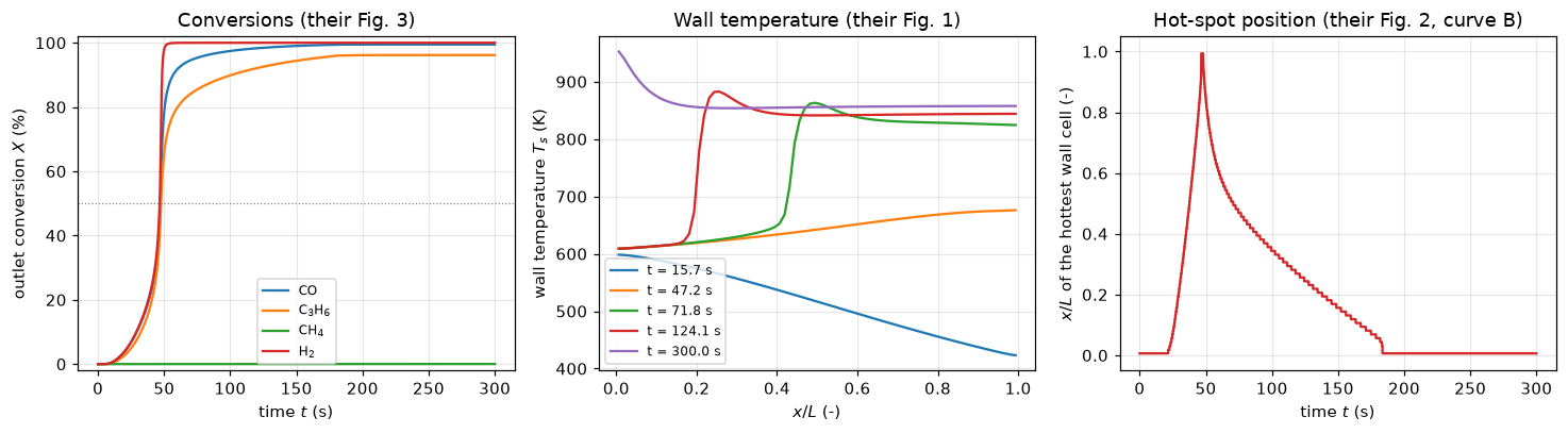
hot-spot position x/L at the times of their Fig. 1: 15.7 s: 0.006, 47.2 s: 0.994, 71.8 s: 0.494, 124.1 s: 0.256, 300 s: 0.006The three panels are the paper’s Figures 3, 1 and 2 in that order, at the five times its Figure 1 is drawn at.
What the paper says in words, and what comes out:
- “their lightoff times (say, the time required for 50 % conversion) are similar except for CH\(_4\)”: CO, C\(_3\)H\(_6\) and H\(_2\) light off within about a second of each other (the spread is printed above); methane stays below 1 % conversion for the whole five minutes.
- “At early times, the hot exhaust heats up the upstream portion of the monolith. As time elapses, however, the downstream section becomes hotter … this temperature peak moves rather slowly toward the inlet” (at the times of their Fig. 1). The hot-spot trace is exactly that: at the inlet while the front is convective, thrown to the outlet at ignition, then walking back upstream over the following four minutes.
- “H\(_2\) in the exhaust leads to a solid temperature exceeding the adiabatic reaction temperature even at steady-state conditions … compare the wall temperature at \(x = 0\) and \(x = 1\)” at the end of the run. Checked numerically in validation 2.
Note what the hot-spot panel costs to draw: the paper’s Figure 2 required re-running the whole transient for each curve.
Case 2: a step decrease in feed temperature, the wrong way
Now the converter starts hot and uniform and is hit with cold exhaust carrying much more hydrocarbon. Cooling the front of the monolith stops the reaction there, so unconverted fuel is delivered to a downstream section that is still hot. The wall temperature goes up.
This is where the paper’s published numbers are, so this run uses the finer grid.
fig, ax = plt.subplots(1, 2, figsize=(9.5, 3.8))
for tt in [2.1, 4.7, 10.1, 14.0]:
    j = int(np.argmin(abs(C2["t"] - tt)))
    ax[0].plot(C2["x_c"], C2["Ts"][j], label=f"t = {C2['t'][j]:.1f} s")
    ax[1].plot(C2["x_c"], 1e2 * C2["yco"][j], label=f"t = {C2['t'][j]:.1f} s")
ax[0].axhline(FEED2.T_s0, color="0.5", lw=0.8, ls=":")
ax[0].set(xlabel="$x/L$ (-)", ylabel="wall temperature $T_s$ (K)",
          title="Wrong-way rise (their Fig. 11)")
ax[1].set(xlabel="$x/L$ (-)", ylabel="gas-phase CO $c_{g}$ (mole %)",
          title="CO breakthrough (their Fig. 12)")
ax[0].legend(fontsize=8)
ax[1].legend(fontsize=8)
fig.tight_layout()
plt.show()
rise = C2["T_max"] - FEED2.T_s0
print(f"transient temperature rise: {rise:.0f} degC   (paper: {PAPER['rise']:.0f} degC)\n"
      f"time of the peak          : {C2['t_peak']:.2f} s (paper: {PAPER['t_peak']:.1f} s)\n"
      f"largest gas temperature over the inlet temperature: {C2['Tg_ratio']:.2f}")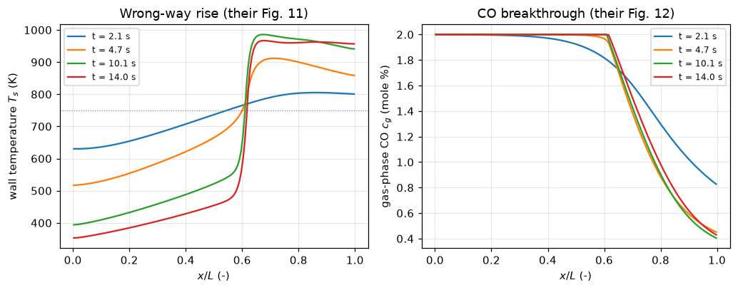
transient temperature rise: 236 degC   (paper: 241 degC)
time of the peak          : 9.73 s (paper: 10.1 s)
largest gas temperature over the inlet temperature: 2.96
The dotted line in the left panel is the initial wall temperature. Everything above it is heat that was not there when the cold gas arrived. The right panel is the mechanism: CO breaks through the quenched front half of the monolith and meets a wall that is still at its initial temperature.
Validation
Five checks, in increasing order of how much they can catch, then the claims and the defect-injection table.
1. Conservation
Two balances that the discretisation should satisfy identically, and will not if the divergence and convection operators are paired wrongly or a boundary term is dropped. What is left is the Newton tolerance, not discretisation error, so these are checks on the assembly rather than on the accuracy.
Species. With the gas quasi-steady, whatever enters and does not leave must have reacted: \(G_{\rm mol}(c^{\rm in}_{g,i} - c^{\rm out}_{g,i}) = \int a\tilde R_i\,dx\) at every instant.
Energy. Over one implicit-Euler step the solid enthalpy change must equal the heat released minus the heat the gas carries out: \(\Delta\!\int(1-\epsilon)\rho_s C_{ps}T_s\,dx = \Delta t\left[\int a\sum(-\Delta H)_i\tilde R_i\,dx - G_{\rm mass}C_{pg}(T_g^{\rm out}-T_g^{\rm in})\right]\), using the adiabatic end condition (eq 15), a term that would not cancel if the zero-gradient wall boundary were wrong.
The outlet value is the one the operator transported. With the outflow outlet the face carries the last cell’s value, so the face value read with compute_boundary_values and the last cell are the same number and both balances close to the Newton tolerance. A zero-gradient outlet dictionary instead extrapolates the face from the interior, a condition the first-order gas equations do not have; on the first minute of case 1 its face differs from the last cell by up to 3e-3 of the feed mole fraction, and a species balance written on the last cell then misses by 0.8 of the smallest molar flux fed (methane’s, the normalisation of the balance below), against below 1e-7 on the face.
print(f"species balance, worst deviation over {len(C1['t'])} time levels : "
      f"below 1e-7 of the smallest species flux fed (here {C1['species']:.1e})\n"
      f"energy balance over {C1['t'][-1]:.0f} s, net closure      : "
      f"below 1e-10 (here {C1['energy_net']:.1e})\n"
      f"                   without cancellation           : "
      f"below 1e-10 (here {C1['energy_abs']:.1e})\n"
      f"total heat released in the transient              : {C1['released']:.1f} J/cm2\n"
      f"zero-gradient outlet, first {TR['zg']['t'][-1]:.0f} s, face against last cell : "
      f"{TR['zg']['face_cell']:.1e} of the feed ({TR['zg']['face_cell_abs']:.1e} in mole fraction)\n"
      f"  species balance written on the last cell         : {TR['zg']['species']:.1e}")
species balance, worst deviation over 3001 time levels : below 1e-7 of the smallest species flux fed (here 5.3e-09)
energy balance over 300 s, net closure : below 1e-10 (here 1.7e-13)
without cancellation : below 1e-10 (here 3.0e-12)
total heat released in the transient : 47118.4 J/cm2
zero-gradient outlet, first 60 s, face against last cell : 3.1e-03 of the feed (4.2e-05 in mole fraction)
species balance written on the last cell : 8.4e-012. The steady state, and the overshoot above it
At long times the solid stops storing heat, so the gas must carry away exactly what the reaction releases, and the outlet gas rise equals \(\sum_i(-\Delta H)_i\,\Delta c_{g,i}/(M C_{pg})\). Agreement here is a statement that the run has genuinely reached steady state at the end of the run, not an independent test of the physics: the two sides are the same balance.
The check that is independent is the one the paper asserts: with H\(_2\) present the wall at the inlet ends up above that adiabatic temperature, because H\(_2\) has a Lewis number near 4 and reaches the wall faster than the heat it liberates can be carried away. Nothing in the model was set up to produce that. The wall temperatures at the two ends are read on the end faces with compute_boundary_values and the wall’s own boundary condition. The inlet value sits on the steep wall profile next to the inlet and is first order in the grid, so the cell below measures its grid error with a 40-cell run.
def overshoot(c1):
    """Wall at the inlet against the adiabatic temperature and against the outlet."""
    st, (ts0, tsl) = c1["steady"], c1["Ts_ends"]
    return dict(ts0=ts0, tsl=tsl, over=ts0 - st["T_ad"],
                holds=bool(ts0 > st["T_ad"] and ts0 > tsl),
                margin=float(min(ts0 - st["T_ad"], ts0 - tsl)))


ST, OV = C1["steady"], overshoot(C1)
C1_N40 = run_case1(n_x=40)          # the coarse level of the wall's grid error


def wall_grid(c_fine, c_coarse, order=1):
    """Richardson estimate of T_s(0) from two grids halved in spacing."""
    t_r = richardson(c_fine["Ts_ends"][0], c_coarse["Ts_ends"][0], order)
    return dict(ts0_rich=t_r, err=t_r - c_fine["Ts_ends"][0],
                over_rich=t_r - c_fine["steady"]["T_ad"])


WG = wall_grid(C1, C1_N40)
print(f"outlet gas temperature rise at t = {C1['t'][-1]:.0f} s : {ST['dT_gas']:7.2f} K\n"
      f"adiabatic rise for that conversion       : {ST['dT_ad']:7.2f} K   "
      f"(difference below 1e-4 %, here {ST['dev_pct']:.0e} %)\n\n"
      f"adiabatic temperature       T_ad       = {ST['T_ad']:7.1f} K\n"
      f"wall temperature at x = 0                = {OV['ts0']:7.1f} K"
      f"   ({OV['over']:+.1f} K vs adiabatic)\n"
      f"wall temperature at x = L                = {OV['tsl']:7.1f} K\n\n"
      f"overshoot above adiabatic at the inlet, and T_s(0) > T_s(L): {OV['holds']}"
      f"  (margin {OV['margin']:.1f} K), both as the paper states for its Fig. 1\n\n"
      f"T_s(0) is first order in the grid: {C1_N40['Ts_ends'][0]:.1f} K on 40 cells, "
      f"{OV['ts0']:.1f} K on 80;\nfirst-order Richardson estimate {WG['ts0_rich']:.1f} K, "
      f"so the 80-cell value is {WG['err']:.1f} K low and the overshoot above T_ad is "
      f"about {WG['over_rich']:.0f} K")
outlet gas temperature rise at t = 300 s : 256.01 K
adiabatic rise for that conversion : 256.01 K (difference below 1e-4 %, here 6e-08 %)
adiabatic temperature T_ad = 856.0 K
wall temperature at x = 0 = 953.9 K (+97.9 K vs adiabatic)
wall temperature at x = L = 857.6 K
overshoot above adiabatic at the inlet, and T_s(0) > T_s(L): True (margin 96.3 K), both as the paper states for its Fig. 1
T_s(0) is first order in the grid: 943.3 K on 40 cells, 953.9 K on 80;
first-order Richardson estimate 964.5 K, so the 80-cell value is 10.6 K low and the overshoot above T_ad is about 108 K3. Table III: the published numbers, nothing fitted
The strongest check the paper pays for. Its Table III gives the peak wall temperature and its location for three solid conductivities spanning two orders of magnitude, and the trend is not monotone in an obvious way: raising \(\lambda_s\) lowers the peak and pushes it downstream.
def table3(T, paper=None):
    """Table III: model against paper, one row per conductivity."""
    paper = PAPER if paper is None else paper
    rows = []
    for k, lam in enumerate(LAM_VALS):
        r = T["tab3"][lam]
        rows.append(dict(lambda_s=lam, T_model=r["T_max"], T_paper=paper["T"][k],
                         dT_pct=100 * (r["T_max"] - paper["T"][k]) / paper["T"][k],
                         x_model=r["x_max"], x_paper=paper["x"][k],
                         dx_cells=(r["x_max"] - paper["x"][k]) * N_PAPER_CELLS,
                         t_peak=r["t_peak"]))
    return pd.DataFrame(rows)


tab3 = table3(TR)
tab3_T_mape = float(np.abs(tab3.dT_pct).mean())
tab3_x_cells = float(np.abs(tab3.dx_cells).max())
trend_T = float(-np.diff(tab3.T_model).max())          # > 0: T falls with lambda
trend_x = float(np.diff(tab3.x_model).min() * 160)     # > 0: x moves downstream, in cells
show = tab3.rename(columns={"lambda_s": "lambda_s (J/cm s K)", "T_model": "T_s,max model (K)",
                            "T_paper": "T_s,max paper (K)", "dT_pct": "dev (%)",
                            "x_model": "x_max/L model", "x_paper": "x_max/L paper",
                            "dx_cells": f"dev (cells of 1/{N_PAPER_CELLS})",
                            "t_peak": "t at peak (s)"})
print(show.round(4).to_string(index=False)
      + f"\n\nmean absolute deviation in T_s,max     : {tab3_T_mape:.2f} %"
      + f"\nworst location deviation               : {tab3_x_cells:.2f} cells "
      f"of the paper's own 1/{N_PAPER_CELLS} grid"
      + f"\nboth trends reproduced: dT/dlambda < 0 and dx/dlambda > 0 -> "
      f"{bool(trend_T > 0 and trend_x > 0)}"
      + f"\n  (smallest temperature step {trend_T:.1f} K, smallest location step "
      f"{trend_x:.0f} cells of 1/160)"
      + f"\nmodel below the paper in {int((tab3.dT_pct < 0).sum())} of 3 rows; "
      f"gap at the standard conductivity {tab3.T_paper[1] - tab3.T_model[1]:.2f} K")
lambda_s (J/cm s K) T_s,max model (K) T_s,max paper (K) dev (%) x_max/L model x_max/L paper dev (cells of 1/80) t at peak (s)
0.0017 990.4409 996.0 -0.5581 0.6656 0.6625 0.25 9.5957
0.0168 986.0591 991.0 -0.4986 0.6719 0.6750 -0.25 9.7262
0.1675 966.8714 975.0 -0.8337 0.7469 0.7625 -1.25 10.2316
mean absolute deviation in T_s,max : 0.63 %
worst location deviation : 1.25 cells of the paper's own 1/80 grid
both trends reproduced: dT/dlambda < 0 and dx/dlambda > 0 -> True
(smallest temperature step 4.4 K, smallest location step 1 cells of 1/160)
model below the paper in 3 of 3 rows; gap at the standard conductivity 4.94 KThe residual is a bias, not scatter, and it is not the grid. All three temperatures come out low by roughly the same fraction, and the refinement study below shows the value at the standard conductivity changes by 1.5 K between 80 and 320 cells while the gap to the paper is 4.9 K. So something small and systematic separates this reimplementation from theirs; the most likely candidates are the four quantities the paper does not print (see Parameters), of which \(Nu_\infty\) moves the peak by 18 K across the three tabulated square-duct values. The page does not claim to have identified which; it claims 0.63 %, and says the sign is consistent.
4. Table III picks between the readings the paper leaves open
Two things had to be decided that the paper does not state outright: the limiting Nusselt/Sherwood number, and whether \(C_{ps}\) sits inside or outside the time derivative. Neither was fitted: each is a choice between a small number of named alternatives, and Table III is the arbiter. This is the same discipline as F2.3: print what each alternative gives and let the paper’s own result choose. The runs use 80 cells, the paper’s grid spacing.
The time of the peak is the more discriminating of the two published quantities here, because the peak temperature is a shallow function of the thermal inertia while the time it takes to get there is not.
def alternatives(T):
    """What each unstated reading gives, against the paper's standard case."""
    labels = {"T": f"Nu=Sh={NU['T']}  (const. wall temperature, T)",
              "H2": f"Nu=Sh={NU['H2']}  (const. flux, axially and peripherally, H2)",
              "H1": f"Nu=Sh={NU['H1']}  (const. axial flux, uniform wall temp., H1)",
              "Cps outside": "H1, but rho*C_ps*dTs/dt instead of d(C_ps Ts)/dt"}
    T_std = PAPER["T"][LAM_VALS.index(LAM_STD)]
    df = pd.DataFrame([dict(variant=labels[k], T_max=r["T_max"], x_max=r["x_max"],
                            t_peak=r["t_peak"]) for k, r in T["alt"].items()])
    df["T_dev_pct"] = 100 * (df.T_max - T_std) / T_std
    df["t_dev_pct"] = 100 * (df.t_peak - PAPER["t_peak"]) / PAPER["t_peak"]
    return df


alt = alternatives(TR)
nu_spread = float(alt.T_max[:3].max() - alt.T_max[:3].min())
print(f"paper: T_s,max = {PAPER['T'][LAM_VALS.index(LAM_STD)]:.0f} K at x/L = "
      f"{PAPER['x'][LAM_VALS.index(LAM_STD)]:.4f}, reached at t = {PAPER['t_peak']} s\n\n"
      + alt.round(3).to_string(index=False)
      + f"\n\nspread of T_s,max over the three Nusselt numbers: {nu_spread:.1f} K")
paper: T_s,max = 991 K at x/L = 0.6750, reached at t = 10.1 s
variant T_max x_max t_peak T_dev_pct t_dev_pct
Nu=Sh=2.976 (const. wall temperature, T) 966.909 0.694 11.293 -2.431 11.813
Nu=Sh=3.091 (const. flux, axially and peripherally, H2) 971.272 0.694 10.996 -1.991 8.873
Nu=Sh=3.608 (const. axial flux, uniform wall temp., H1) 984.909 0.681 9.730 -0.615 -3.663
H1, but rho*C_ps*dTs/dt instead of d(C_ps Ts)/dt 978.952 0.681 7.828 -1.216 -22.492
spread of T_s,max over the three Nusselt numbers: 18.0 K5. Grid and time-step independence of a moving front
The light-off time and the peak location are both properties of a front that moves through the grid, so neither means anything until it stops changing under refinement. The front is where the solution is steepest, so the light-off time (the instant the ignition front reaches the outlet conversion of 50 %) is the quantity on which the grid error is measured. The paper’s own \(x_{\max}/L\) values are exact multiples of the spacing of its grid (The data), so its location is quantised to one cell and cannot be compared more finely than that.
Case 1 is refined on the light-off time, case 2 on the peak temperature. Both schemes are first order in space (upwind) and in time (backward Euler). The light-off time moves monotonically under both refinements. The case-2 peak temperature does not: over the grid it falls and then rises again, because its location is a cell centre and jumps between cells as the grid changes, so the spreads below measure how much the numbers move over this ladder; they are not bounds on the discretisation error. The time of the peak moves monotonically with the step, and a first-order Richardson estimate from the two finest steps gives its step-converged value and the paper deviation of that value.
def ladder1(T):
    """Light-off time of CO over grid and time step."""
    return pd.DataFrame([dict(n_x=n, dt=d, t_lightoff=v) for (n, d), v in T["lad1"].items()])


def ladder2(T):
    """Peak wall temperature over grid and time step, standard conductivity."""
    return pd.DataFrame([dict(n_x=n, dt=d, T_max=r["T_max"], x_max=r["x_max"], t_peak=r["t_peak"])
                         for (n, d), r in T["lad2"].items()])


def spreads(T):
    """The three refinement spreads."""
    l1, l2 = ladder1(T), ladder2(T)
    g, d = l2[l2.dt == 0.05], l2[l2.n_x == 160]
    lo = float(l1.t_lightoff.max() - l1.t_lightoff.min())
    return dict(lo=lo, lo_pct=100 * lo / T["lad1"][(80, 0.1)],
                grid=float(g.T_max.max() - g.T_max.min()),
                dt=float(d.T_max.max() - d.T_max.min()),
                g80_320=float(abs(T["lad2"][(320, 0.05)]["T_max"] - T["lad2"][(80, 0.05)]["T_max"])),
                t_peak_rich=richardson(T["lad2"][(160, 0.025)]["t_peak"],
                                       T["lad2"][(160, 0.05)]["t_peak"]))


conv1, conv2, SP = ladder1(TR), ladder2(TR), spreads(TR)
print("CASE 1 - time to 50 % CO conversion (root-found)\n"
      + conv1.round(3).to_string(index=False)
      + f"\nspread over a 4x grid change and a 4x time-step change: {SP['lo']:.2f} s "
      f"({SP['lo_pct']:.1f} % of {TR['lad1'][(80, 0.1)]:.1f} s)")
CASE 1 - time to 50 % CO conversion (root-found)
n_x dt t_lightoff
40 0.10 47.424
80 0.20 47.279
80 0.10 47.123
80 0.05 47.044
160 0.10 46.974
spread over a 4x grid change and a 4x time-step change: 0.45 s (1.0 % of 47.1 s)print("CASE 2 - peak wall temperature at the standard conductivity (refined in time)\n"
+ conv2.round(4).to_string(index=False)
+ f"\n\nspread over n_x = 40 -> 320 at dt = 0.05 : {SP['grid']:.2f} K"
+ f"\nspread over dt = 0.1 -> 0.025 at n_x = 160: {SP['dt']:.2f} K"
+ f"\nchange between 80 and 320 cells : {SP['g80_320']:.2f} K"
+ f"\ntime of the peak, n_x = 160: {TR['lad2'][(160, 0.05)]['t_peak']:.3f} s at dt = 0.05, "
f"first-order Richardson from dt = 0.05 and 0.025: {SP['t_peak_rich']:.3f} s,"
f"\n {100 * (PAPER['t_peak'] - SP['t_peak_rich']) / PAPER['t_peak']:.2f} % before the "
f"paper's {PAPER['t_peak']} s")CASE 2 - peak wall temperature at the standard conductivity (refined in time)
n_x dt T_max x_max t_peak
40 0.050 989.6493 0.6875 9.9796
80 0.050 984.9092 0.6812 9.7300
160 0.100 986.1280 0.6781 9.6574
160 0.050 986.0591 0.6719 9.7262
160 0.025 986.0102 0.6719 9.7433
320 0.050 986.3915 0.6734 9.6810
spread over n_x = 40 -> 320 at dt = 0.05 : 4.74 K
spread over dt = 0.1 -> 0.025 at n_x = 160: 0.12 K
change between 80 and 320 cells : 1.48 K
time of the peak, n_x = 160: 9.726 s at dt = 0.05, first-order Richardson from dt = 0.05 and 0.025: 9.760 s,
3.36 % before the paper's 10.1 sClaims
Every number the page states, registered once with how it is checked (docs/claims-design.md). Values above round-off are held to tolerances well above their spread across BLAS kernels but tight enough for the defect rows to fail them; the balance closures are bounds set by the Newton tolerance.
def flat(T):
    """The transient claims of a run of ``transient``, as ``{name: value}``."""
    c1, st = T["c1"], T["c1"]["steady"]
    ov, t3, al, sp = overshoot(c1), table3(T), alternatives(T), spreads(T)
    k_std = LAM_VALS.index(LAM_STD)
    out = {f"lightoff_{s}_s": c1["t_lo"][s] for s in ("CO", "C3H6", "H2") if s in c1["t_lo"]}
    out["lightoff_species_spread_s"] = (max(out.values()) - min(out.values()))
    out.update(ch4_max_conversion=c1["ch4_max_X"], species_balance_closure=c1["species"],
               energy_balance_net_closure=c1["energy_net"],
               energy_balance_abs_closure=c1["energy_abs"],
               heat_released_J_per_cm2=c1["released"], steady_dT_gas_K=st["dT_gas"],
               steady_dT_ad_K=st["dT_ad"], steady_adiabatic_dev_pct=st["dev_pct"],
               T_ad_K=st["T_ad"], Ts_inlet_K=ov["ts0"], Ts_outlet_K=ov["tsl"],
               overshoot_K=ov["over"], overshoot_as_paper_states=ov["holds"])
    out.update({f"hotspot_x_at_{tt:g}s": x for tt, x in c1["hot_x"].items()})
    out.update(zero_gradient_face_cell_gap=T["zg"]["face_cell"],
               zero_gradient_face_cell_gap_abs=T["zg"]["face_cell_abs"],
               zero_gradient_species_closure_cell=T["zg"]["species"])
    for k, lam in enumerate(LAM_VALS):
        tag = f"{lam:.3e}"
        out[f"table3_T_model_{tag}"] = t3.T_model[k]
        out[f"table3_x_model_{tag}"] = t3.x_model[k]
        out[f"table3_t_peak_{tag}"] = t3.t_peak[k]
        out[f"table3_dT_pct_{tag}"] = t3.dT_pct[k]
        out[f"table3_dx_cells_{tag}"] = t3.dx_cells[k]
    r_std = T["tab3"][LAM_STD]
    out.update(table3_T_mean_abs_dev_pct=float(np.abs(t3.dT_pct).mean()),
               table3_x_max_dev_cells=float(np.abs(t3.dx_cells).max()),
               t_peak_dev_pct=100 * abs(r_std["t_peak"] - PAPER["t_peak"]) / PAPER["t_peak"],
               temperature_rise_K=r_std["T_max"] - FEED2.T_s0,
               temperature_rise_dev_pct=100 * abs(r_std["T_max"] - FEED2.T_s0 - PAPER["rise"])
               / PAPER["rise"],
               table3_gap_to_paper_std_K=PAPER["T"][k_std] - r_std["T_max"],
               case2_velocity_ratio=r_std["Tg_ratio"],
               table3_trends_reproduced=bool(np.all(np.diff(t3.T_model) < 0)
                                             and np.all(np.diff(t3.x_model) > 0)))
    for k, key in enumerate(T["alt"]):
        tag = key.replace(" ", "_")
        out[f"alt_T_max_{tag}"] = al.T_max[k]
        out[f"alt_x_max_{tag}"] = al.x_max[k]
        out[f"alt_t_peak_{tag}"] = al.t_peak[k]
        out[f"alt_T_dev_pct_{tag}"] = al.T_dev_pct[k]
        out[f"alt_t_dev_pct_{tag}"] = al.t_dev_pct[k]
    out["alt_nu_spread_K"] = float(al.T_max[:3].max() - al.T_max[:3].min())
    for (n, d), v in T["lad1"].items():
        out[f"lightoff_n{n}_dt{d:g}_s"] = v
    for (n, d), r in T["lad2"].items():
        for q in ("T_max", "x_max", "t_peak"):
            out[f"case2_{q}_n{n}_dt{d:g}"] = r[q]
    out.update(lightoff_grid_dt_spread_s=sp["lo"], lightoff_grid_dt_spread_pct=sp["lo_pct"],
               case2_grid_spread_K=sp["grid"], case2_dt_spread_K=sp["dt"],
               case2_change_80_320_K=sp["g80_320"],
               t_peak_dt_richardson_s=sp["t_peak_rich"],
               t_peak_dt_richardson_dev_pct=100 * (PAPER["t_peak"] - sp["t_peak_rich"])
               / PAPER["t_peak"])
    return out


def register(claims, vals):
    """Register the transient claims with the check each needs."""
    bounds = {"species_balance_closure": (1e-7, "tolerance", "newton tol 1e-9 on scaled unknowns"),
              "energy_balance_net_closure": (1e-10, "tolerance", "newton tol 1e-9"),
              "energy_balance_abs_closure": (1e-10, "tolerance", "newton tol 1e-9"),
              "steady_adiabatic_dev_pct": (1e-4, "chosen",
                                           "the solid stores no heat at the end of the run")}
    for name, v in vals.items():
        if name in bounds:
            mx, basis, note = bounds[name]
            claims.bound(name, v, max=mx, basis=basis, note=note)
        elif name == "overshoot_as_paper_states":
            claims.exact(name, v, margin=OV["margin"], min_margin=10.0,
                         note="margin in K: min(T_s(0) - T_ad, T_s(0) - T_s(L))")
        elif name == "table3_trends_reproduced":
            claims.exact(name, v, margin=min(trend_T, trend_x), min_margin=0.5,
                         note="margin: smallest step, in K and in cells of 1/160")
        elif "dx_cells" in name or name == "table3_x_max_dev_cells":
            claims.value(name, v, rtol=1e-4, note="multiples of a quarter cell of 1/80")
        elif "x_max" in name or "x_model" in name or "hotspot" in name:
            claims.value(name, v, rtol=1e-6, note="a cell centre")
        elif "spread" in name or "change" in name or "dev_pct" in name or "gap" in name:
            claims.value(name, v, rtol=1e-2)
        elif "zero_gradient" in name:
            claims.value(name, v, rtol=1e-2)
        else:
            claims.value(name, v, rtol=1e-4)


V = flat(TR)
register(claims, V)
claims.count("table3_rows_below_paper", tab3.T_model - tab3.T_paper, 0.0, above=False,
             min_margin=1.0, relative=False, note="margin in K")

# the static claims: data, geometry, properties
paper_claims = {"paper_T_s_max_" + f"{lam:.3e}": PAPER["T"][k] for k, lam in enumerate(LAM_VALS)}
paper_claims.update({"paper_x_max_" + f"{lam:.3e}": PAPER["x"][k] for k, lam in enumerate(LAM_VALS)})
paper_claims.update(paper_t_peak_s=PAPER["t_peak"], paper_temperature_rise_K=PAPER["rise"],
                    paper_lewis_H2=PAPER["Le_H2"])
for name, v in paper_claims.items():
    claims.value(name, v, rtol=1e-9, note="read from the results file")
claims.exact("paper_grid_points", int(PAPER["n_grid"]))
claims.bound("paper_x_max_on_grid", x_on_grid, max=1e-9, basis="identity",
             note="the sidecar's finding: x_max/L are multiples of 1/80")
stated = {"stated_T_s0_case1_K": FEED1.T_s0, "stated_T_g_in_case1_K": FEED1.T_g_in,
          "stated_T_s0_case2_K": FEED2.T_s0, "stated_T_g_in_case2_K": FEED2.T_g_in,
          "stated_y_CH4_case1": FEED1.y_in[2]}
for name, v in stated.items():
    claims.value(name, v, rtol=1e-9, note="Table I, read from the parameter file")
claims.value("table2_geometry_max_dev_pct", geo_max_err, rtol=1e-3)
for k in range(len(geo_chk)):
    tag = f"{geo_chk.cell_density_per_cm2[k]:g}"
    for col in ("R_h_calc", "eps_calc", "R_h_err_pct", "eps_err_pct"):
        claims.value(f"table2_{col}_{tag}", geo_chk[col][k], rtol=1e-6)
for s in SPECIES:
    claims.value(f"lewis_{s}", GP["le"][s], rtol=1e-6)
claims.value("lewis_H2_dev_pct", 100 * abs(LE_H2 - PAPER["Le_H2"]) / PAPER["Le_H2"], rtol=1e-4)
claims.value("s_geo_cm2_per_cm3", PRM.s_geo, rtol=1e-9)
claims.value("gas_residence_time_ms", GP["tau_res"] * 1e3, rtol=1e-6)
claims.value("h_600K_W_per_cm2_K", GP["h"], rtol=1e-6)
claims.value("wall_time_constant_s", GP["tau_wall"], rtol=1e-6)
claims.value("inertia_ratio_300K", INERTIA_300, rtol=1e-6)
claims.value("state_span_decades", state_decades, rtol=1e-6)
claims.bound("lightoff_interp_minus_root_s", LO_INTERP_GAP, max=1e-2, basis="chosen",
             note="interpolation between levels is within 1e-2 s of the root at dt 0.1 s")
claims.value("Ts_inlet_richardson_K", WG["ts0_rich"], rtol=1e-4)
claims.value("Ts_inlet_grid_error_80_K", WG["err"], rtol=1e-2)
claims.value("overshoot_richardson_K", WG["over_rich"], rtol=1e-4)
claims.value("unbounded_first_step_min_y", y_min_unbounded_guarded, rtol=1e-3,
             note="the negative root that full steps reach without bounds")
claims.bound("bounded_first_step_min_y", y_min_bounded, min=0.0, basis="theory",
             note="mole fractions held in [0, y_in] by the bounds")
print(f"{len(claims.metrics)} claims registered")
147 claims registeredThe defect-injection table
Each row breaks one thing on purpose, re-runs the computation behind its claims with the defect in place, and hands the result to claims.breaks, which records whether the claim’s own check catches it. Every claim that is not structural must be failed by at least one row, and the last cell of the page raises otherwise. The first row re-runs every transient result on the page. Rows that leave a claim inside its check are listed too; the table after it says why each such pair is not caught.
BREAK = []


def brk(row, name, value):
    """One injected defect: ``value`` is what claim ``name`` becomes with it."""
    BREAK.append((row, name, value, claims.breaks(row, name, value)))


# 1. thermochemistry: the heats of combustion with liquid product water
row = "heats of combustion with liquid water"
TR_liq = transient(dh=heats_of_combustion("liquid"))
V_liq = flat(TR_liq)
for name, v in V_liq.items():
    brk(row, name, v)
brk(row, "table3_rows_below_paper", int((table3(TR_liq).dT_pct < 0).sum()))

# 2. the overshoot needs the hydrogen (Le near 4): case 1 re-run without it
row = "no hydrogen in the case-1 feed"
y_noh2 = list(FEED1.y_in)
y_noh2[3] = 0.0
c1_noh2 = run_case1(feed=replace(FEED1, y_in=tuple(y_noh2)))
for name, v in flat(dict(TR, c1=c1_noh2)).items():
    if name in ("overshoot_as_paper_states", "T_ad_K", "Ts_inlet_K", "Ts_outlet_K",
                "overshoot_K", "hotspot_x_at_300s", "steady_dT_ad_K", "steady_dT_gas_K"):
        brk(row, name, v)

# 3. the early hot spot sits at the inlet because the gas entering there is hotter
row = "case 1 with case 2's wall and inlet temperatures (first 20 s)"
c1_hot = run_case1(feed=replace(FEED1, T_s0=FEED2.T_s0, T_g_in=FEED2.T_g_in), t_end=20.0)
brk(row, "hotspot_x_at_15.7s", c1_hot["hot_x"][15.7])

# 4. the trends of Table III: the conductivities parsed without their exponent
row = "Table III conductivities read without their exponent"
lam_bad = [float(f"{lam:.3e}".split("e")[0]) for lam in LAM_VALS]
runs_bad = {lb: run_case2(params=replace(PRM, lam_s=lb)) for lb in set(lam_bad)}
tab3_bad = table3(dict(TR, tab3={lam: runs_bad[lb] for lam, lb in zip(LAM_VALS, lam_bad)}))
brk(row, "table3_trends_reproduced",
    bool(np.all(np.diff(tab3_bad.T_model) < 0) and np.all(np.diff(tab3_bad.x_model) > 0)))

# 5. the balances on the last cell of a zero-gradient outlet
row = "outlet as zero gradient, balances on the last cell"
for name, key in (("species_balance_closure", "species"),
                  ("energy_balance_net_closure", "energy_net"),
                  ("energy_balance_abs_closure", "energy_abs")):
    brk(row, name, TR["zg"][key])

# 6. the steady-state check taken before steady state
row = "steady-state check taken at 60 s"
brk(row, "steady_adiabatic_dev_pct", steady_check(C1["model"], C1["march"], t_check=60.0)["dev_pct"])

# 7. the zero-gradient comparison run with the outflow outlet instead
row = "outflow outlet in the zero-gradient comparison"
c1_of = run_case1(t_end=60.0, outlet="outflow", read="cell")
brk(row, "zero_gradient_species_closure_cell", c1_of["species"])
brk(row, "zero_gradient_face_cell_gap", c1_of["face_cell"])
brk(row, "zero_gradient_face_cell_gap_abs", c1_of["face_cell_abs"])

# 8. the data files read one row off
row = "results file read one row off"
P_off = paper_results(res, offset=1)
for k, lam in enumerate(LAM_VALS):
    brk(row, f"paper_T_s_max_{lam:.3e}", P_off["T"][k])
    brk(row, f"paper_x_max_{lam:.3e}", P_off["x"][k])
brk(row, "paper_t_peak_s", P_off["t_peak"])
brk(row, "paper_temperature_rise_K", P_off["rise"])
brk(row, "paper_lewis_H2", P_off["Le_H2"])
brk(row, "paper_grid_points", int(P_off["n_grid"]))
row = "paper's spacing taken as L / 81 (points for intervals)"
xs = np.array(PAPER["x"]) * PAPER["n_grid"]
brk(row, "paper_x_max_on_grid", float(np.max(np.abs(xs - np.round(xs)))))
row = "parameter file read one row off"
P1 = table_lookup(par, offset=1)
F1o, F2o = Feed.from_table(P1, "case 1"), Feed.from_table(P1, "case 2")
for name, v in {"stated_T_s0_case1_K": F1o.T_s0, "stated_T_g_in_case1_K": F1o.T_g_in,
                "stated_T_s0_case2_K": F2o.T_s0, "stated_T_g_in_case2_K": F2o.T_g_in,
                "stated_y_CH4_case1": F1o.y_in[2]}.items():
    brk(row, name, v)
brk(row, "state_span_decades", float(np.log10(F2o.T_s0 / F1o.y_in[2])))

# 9. geometry: R_h as the full open side; void fraction not squared
row = "R_h taken as the open side (the usual hydraulic diameter)"
g_bad = table2_check(geo, rh_of_side=lambda s: s)
brk(row, "table2_geometry_max_dev_pct",
    float(np.abs(g_bad[["R_h_err_pct", "eps_err_pct"]].to_numpy()).max()))
row = "void fraction as s/p, not squared"
g_bad2 = table2_check(geo, eps_power=1)
for k in range(len(geo_chk)):
    tag = f"{geo_chk.cell_density_per_cm2[k]:g}"
    brk("R_h taken as the open side (the usual hydraulic diameter)", f"table2_R_h_calc_{tag}",
        g_bad.R_h_calc[k])
    brk("R_h taken as the open side (the usual hydraulic diameter)", f"table2_R_h_err_pct_{tag}",
        g_bad.R_h_err_pct[k])
    brk(row, f"table2_eps_calc_{tag}", g_bad2.eps_calc[k])
    brk(row, f"table2_eps_err_pct_{tag}", g_bad2.eps_err_pct[k])
brk("R_h taken as the open side (the usual hydraulic diameter)", "s_geo_cm2_per_cm3",
    2 * PRM.eps / (2 * PRM.r_h))

# 10. gas properties: the exhaust taken as nitrogen; R_h read as a radius
row = "exhaust molecular weight taken as nitrogen's"
GP_n2 = gas_properties(m_gas=MW["N2"])
for s in SPECIES:
    brk(row, f"lewis_{s}", GP_n2["le"][s])
brk(row, "lewis_H2_dev_pct", 100 * abs(GP_n2["le"]["H2"] - PAPER["Le_H2"]) / PAPER["Le_H2"])
brk(row, "gas_residence_time_ms", GP_n2["tau_res"] * 1e3)
row = "R_h read as a radius: transfer length R_h instead of 2 R_h"
GP_rh = gas_properties(transfer_length=PRM.r_h)
brk(row, "h_600K_W_per_cm2_K", GP_rh["h"])
brk(row, "wall_time_constant_s", GP_rh["tau_wall"])
row = "C_ps derivative with the sign of its c2 term flipped"
brk(row, "inertia_ratio_300K", inertia_ratio(FEED1.T_s0, cps=(PRM.cps[0], PRM.cps[1], -PRM.cps[2])))

# 11. the bounds removed, with full steps or with monotone damping
row = "all bounds removed, guarded full steps"
brk(row, "bounded_first_step_min_y", y_min_unbounded_guarded)
row = "all bounds removed, monotone damping"
brk(row, "unbounded_first_step_min_y", y_min_unbounded)

# 12. the scaling removed: physical units, newton's tolerances on raw unknowns
row = "two-sided scaling removed"
c1_raw = run_case1(t_end=60.0, scaled=False)
brk(row, "species_balance_closure", c1_raw["species"])

print(f"species balance without the scaling, first 60 s: {c1_raw['species']:.1e} "
      "(the bound is 1e-7)")
# 13. Richardson estimates taken as second order; light-off read at the nearest level
row = "Richardson extrapolation taken as second order"
WG2 = wall_grid(C1, C1_N40, order=2)
brk(row, "Ts_inlet_richardson_K", WG2["ts0_rich"])
brk(row, "Ts_inlet_grid_error_80_K", WG2["err"])
brk(row, "overshoot_richardson_K", WG2["over_rich"])
t_r2 = richardson(TR["lad2"][(160, 0.025)]["t_peak"], TR["lad2"][(160, 0.05)]["t_peak"], order=2)
brk(row, "t_peak_dt_richardson_s", t_r2)
brk(row, "t_peak_dt_richardson_dev_pct", 100 * (PAPER["t_peak"] - t_r2) / PAPER["t_peak"])
row = "light-off read at the nearest time level"
brk(row, "lightoff_interp_minus_root_s", abs(lightoff_by_level(C1, method="nearest")
                                             - C1["t_lo"]["CO"]))

tbl = pd.DataFrame(BREAK, columns=["row", "claim", "broken value", "caught"])
summary = tbl.groupby("row", sort=False).agg(claims=("claim", "size"), caught=("caught", "sum"))
print(summary.to_string())
species balance without the scaling, first 60 s: 1.5e-10 (the bound is 1e-7)
claims caught
row
heats of combustion with liquid water 100 92
no hydrogen in the case-1 feed 8 8
case 1 with case 2's wall and inlet temperatures (first 20 s) 1 1
Table III conductivities read without their exponent 1 1
outlet as zero gradient, balances on the last cell 3 3
steady-state check taken at 60 s 1 1
outflow outlet in the zero-gradient comparison 3 3
results file read one row off 10 10
paper's spacing taken as L / 81 (points for intervals) 1 1
parameter file read one row off 6 6
R_h taken as the open side (the usual hydraulic diameter) 8 8
void fraction as s/p, not squared 6 6
exhaust molecular weight taken as nitrogen's 7 7
R_h read as a radius: transfer length R_h instead of 2 R_h 2 2
C_ps derivative with the sign of its c2 term flipped 1 1
all bounds removed, guarded full steps 1 1
all bounds removed, monotone damping 1 1
two-sided scaling removed 1 0
Richardson extrapolation taken as second order 5 5
light-off read at the nearest time level 1 1Pairs a row leaves inside the claim’s check are expected wherever the row’s defect does not enter the quantity. In row 1 (a physics defect, everything re-run): the three balance closures and the steady-state check are identities of the discretisation and of the steady state, so they cannot move, only a defect in how the outlet is read (row 5) or in when the check is taken (row 6) moves them; the overshoot label and the Table III trends are true/false claims with margins of tens of kelvin and a cell, which the heat of condensation does not flip (rows 2 and 4 do); the hot spot at 300 s stays on the inlet cell because the H2 overshoot pins it there, and only removing the hydrogen (row 2) moves it; the early hot spot is on the inlet cell because the gas entering there is hotter than the wall (row 3, cold gas on a hot wall, moves it). Row 12 checks only the species balance, over the first 60 s rather than the 300 s of the claim; without the scaling it still closes inside its bound, so the scaling is a convenience here, not a necessity. The cell below prints the count and every uncaught pair; every claim that is not structural is caught by at least one row.
unc = tbl[~tbl.caught]
print(f"{int(tbl.caught.sum())} of {len(tbl)} pairs caught; {len(unc)} uncaught:\n"
      + "\n".join(f"  {r}: " + ", ".join(unc.claim[unc.row == r])
                  for r in dict.fromkeys(unc.row)))
158 of 167 pairs caught; 9 uncaught:
heats of combustion with liquid water: species_balance_closure, energy_balance_net_closure, energy_balance_abs_closure, steady_adiabatic_dev_pct, overshoot_as_paper_states, hotspot_x_at_15.7s, hotspot_x_at_300s, table3_trends_reproduced
two-sided scaling removed: species_balance_closureWhat pymrm adds
The physics is entirely theirs. No equation on this page is new, no parameter was re-estimated, and the agreement numbers above are agreement with a 1982 reference solution, not with experiment.
What changes is the shape of the calculation. The paper’s Section “Numerical Solution of the Equations” describes a bespoke architecture, and it is a fair amount of machinery: a Galerkin discretisation of the solid energy equation in piecewise-linear basis functions (their eqs 23 and 24), reduced to \(B(\bar T_s)\,\mathrm{d}\bar T_s/\mathrm{d}t = F(\bar T_s,t)\); a banded GEAR integrator for that; and, inside every right-hand-side evaluation, a march down the channel solving eq 25 for \(T_g\) cell by cell and then the coupled pair eqs 26 and 27 for \(c_g\) and \(c_s\) by Newton’s method at each cell. Two nested nonlinear solves inside a stiff ODE integrator, and a Jacobian the paper has to argue is “well approximated by a banded tridiagonal matrix” because strictly it is not banded at all.
Here that structure disappears. The conduction and convection operators are assembled once by construct_grad, construct_div and construct_convflux_upwind; NumJac supplies the pointwise block Jacobian for reaction, film transfer and accumulation together; and one newton call per time step solves all twelve fields simultaneously, with bounds keeping it on the physical root and every step’s convergence checked. The Jacobian has the full sparse structure of the coupled system, analytic in the constant operators and differenced by NumJac in the pointwise terms, so no coupling is dropped, and the nesting is gone because there is nothing left to nest.
Two things follow that are more than tidiness:
- The refinement study above is affordable, at four grids and four time steps. In 1982 that was the reason to fix the grid and not ask the question, and the paper’s own \(x_{\max}/L\) values still carry the fingerprint of that grid, being exact multiples of its spacing.
- Two unstated modelling choices become testable rather than assumed. The limiting Nusselt number and the placement of \(C_{ps}\) inside or outside the time derivative are both decided here by running the alternatives against Table III, which is only practical when a variant is cheap.
What it does not add: nothing here would change an engineering conclusion of the original paper. The value is that the model is now a short model.py that anyone can re-run and perturb, rather than a Fortran program in a General Motors report.
Reuse
The structure (a quasi-steady fluid phase convecting past a solid phase that stores heat and carries the reaction, coupled by film transfer) is not specific to converters. To move it to another system, change three things and nothing else:
Monolith.ratesand the heats of combustion (dh=) for different chemistry, withMonolith._build_scaling’s bounds set to the range each new species can take;- the carrier velocities in
Monolith._build_operators(they are the only place the hydrodynamics enters, and both are constants because mass and molar flux are conserved even when \(u\) is not); Monolith.enthalpyandOhCavendish.lam_sfor a different substrate.
The parts worth lifting as they are:
- The single-field diffusion trick. A coefficient matrix that is non-zero on one field only gives that field a diffusion term inside a monolithic system, without building a separate operator or a separate solve.
{"outflow": True}for the convected fields. An equation first order in \(x\) has no outlet condition; the outflow marker gives the face the last cell’s value, so balances close on it, while a zero-gradient dictionary imposes a condition the equation does not have.- Bounds where the residual has more than one root. With an inhibition denominator like \(G\), full Newton steps can converge to a root with negative mole fractions;
bounds=at zero keeps the solve on the physical one.
Related pages: D2.2 for the steady-state runaway boundary of the same competition between heat release and heat removal, and B1.1 for what happens when the same balance is drawn on a single particle instead of a channel.
Reference. Oh, S. H.; Cavendish, J. C. Transients of monolithic catalytic converters: response to step changes in feedstream temperature as related to controlling automobile emissions. Ind. Eng. Chem. Prod. Res. Dev. 1982, 21(1), 29 to 37. doi:10.1021/i300005a006
# prose literals: the notebook text above, then meta.yaml and the models.yaml entry
for lit, name in [
    # introduction and background
    ("241", "paper_temperature_rise_K"), ("236", "temperature_rise_K"),
    ("9", "gas_residence_time_ms"), ("3", "wall_time_constant_s"),
    # the published model and the parameters
    ("2.1", "inertia_ratio_300K"), ("300", "stated_T_s0_case1_K"),
    ("81", "paper_grid_points"),
    # implementation
    ("3.0", "case2_velocity_ratio"), ("7", "state_span_decades"),
    ("750", "stated_T_s0_case2_K"), ("5e-5", "stated_y_CH4_case1"),
    # results
    ("below 1 %", "ch4_max_conversion"),
    # validation
    ("3e-3", "zero_gradient_face_cell_gap"), ("0.8", "zero_gradient_species_closure_cell"),
    ("below 1e-7", "species_balance_closure"),
    ("1.5", "case2_change_80_320_K"), ("4.9", "table3_gap_to_paper_std_K"),
    ("18", "alt_nu_spread_K"), ("0.63", "table3_T_mean_abs_dev_pct"),
]:
    claims.says(lit, name)
# meta.yaml (validation, adds, agreement, caveats) and the models.yaml entry
for lit, name in [
("0.09", "table2_geometry_max_dev_pct"), ("below 1e-7", "species_balance_closure"),
("below 1e-10", "energy_balance_net_closure"), ("below 1e-10", "energy_balance_abs_closure"),
("0.63", "table3_T_mean_abs_dev_pct"), ("990.4", "table3_T_model_1.675e-03"),
("986.1", "table3_T_model_1.675e-02"), ("966.9", "table3_T_model_1.675e-01"),
("996", "paper_T_s_max_1.675e-03"), ("991", "paper_T_s_max_1.675e-02"),
("975", "paper_T_s_max_1.675e-01"), ("1.25", "table3_x_max_dev_cells"),
("236", "temperature_rise_K"), ("241", "paper_temperature_rise_K"),
("9.73", "table3_t_peak_1.675e-02"), ("10.1", "paper_t_peak_s"),
("3.89", "lewis_H2"), ("4", "paper_lewis_H2"), ("47.12", "lightoff_CO_s"),
("0.45", "lightoff_grid_dt_spread_s"), ("1.0", "lightoff_grid_dt_spread_pct"),
("1.5", "case2_change_80_320_K"), ("4.9", "table3_gap_to_paper_std_K"),
("-0.5", "table3_dT_pct_1.675e-02"), ("-0.8", "table3_dT_pct_1.675e-01"),
("97.9", "overshoot_K"), ("3.70", "t_peak_dev_pct"),
("108", "overshoot_richardson_K"), ("9.76", "t_peak_dt_richardson_s"),
("3.4", "t_peak_dt_richardson_dev_pct"),
]:
claims.says(lit, name)# Claims: prints every registered number, writes agreement.json for CI, and
# raises when a claim fails its own check or has no break row.
claims.report(); # the semicolon keeps the notebook from echoing the payloadClaims for I1.2:
lightoff_CO_s = 47.123 value rtol 0.0001
lightoff_C3H6_s = 47.624 value rtol 0.0001
lightoff_H2_s = 46.617 value rtol 0.0001
lightoff_species_spread_s = 1.0071 value rtol 0.01
ch4_max_conversion = 0.00029759 value rtol 0.0001
species_balance_closure = (here 5.3e-09) bound bound <= 1e-07 [tolerance]
energy_balance_net_closure = (here 1.7e-13) bound bound <= 1e-10 [tolerance]
energy_balance_abs_closure = (here 3.0e-12) bound bound <= 1e-10 [tolerance]
heat_released_J_per_cm2 = 47118 value rtol 0.0001
steady_dT_gas_K = 256.01 value rtol 0.0001
steady_dT_ad_K = 256.01 value rtol 0.0001
steady_adiabatic_dev_pct = (here 5.6e-08) bound bound <= 0.0001 [chosen]
T_ad_K = 856.01 value rtol 0.0001
Ts_inlet_K = 953.89 value rtol 0.0001
Ts_outlet_K = 857.56 value rtol 0.0001
overshoot_K = 97.88 value rtol 0.0001
overshoot_as_paper_states = True exact exact, margin 96.3
hotspot_x_at_15.7s = 0.00625 value rtol 1e-06
hotspot_x_at_47.2s = 0.99375 value rtol 1e-06
hotspot_x_at_71.8s = 0.49375 value rtol 1e-06
hotspot_x_at_124.1s = 0.25625 value rtol 1e-06
hotspot_x_at_300s = 0.00625 value rtol 1e-06
zero_gradient_face_cell_gap = 0.0030935 value rtol 0.01
zero_gradient_face_cell_gap_abs = 4.1932e-05 value rtol 0.01
zero_gradient_species_closure_cell = 0.83864 value rtol 0.01
table3_T_model_1.675e-03 = 990.44 value rtol 0.0001
table3_x_model_1.675e-03 = 0.66563 value rtol 1e-06
table3_t_peak_1.675e-03 = 9.5957 value rtol 0.0001
table3_dT_pct_1.675e-03 = -0.55815 value rtol 0.0001
table3_dx_cells_1.675e-03 = 0.25 value rtol 0.0001
table3_T_model_1.675e-02 = 986.06 value rtol 0.0001
table3_x_model_1.675e-02 = 0.67188 value rtol 1e-06
table3_t_peak_1.675e-02 = 9.7262 value rtol 0.0001
table3_dT_pct_1.675e-02 = -0.49857 value rtol 0.0001
table3_dx_cells_1.675e-02 = -0.25 value rtol 0.0001
table3_T_model_1.675e-01 = 966.87 value rtol 0.0001
table3_x_model_1.675e-01 = 0.74687 value rtol 1e-06
table3_t_peak_1.675e-01 = 10.232 value rtol 0.0001
table3_dT_pct_1.675e-01 = -0.8337 value rtol 0.0001
table3_dx_cells_1.675e-01 = -1.25 value rtol 0.0001
table3_T_mean_abs_dev_pct = 0.63014 value rtol 0.01
table3_x_max_dev_cells = 1.25 value rtol 0.0001
t_peak_dev_pct = 3.7009 value rtol 0.01
temperature_rise_K = 236.06 value rtol 0.0001
temperature_rise_dev_pct = 2.0502 value rtol 0.01
table3_gap_to_paper_std_K = 4.9409 value rtol 0.01
case2_velocity_ratio = 2.958 value rtol 0.0001
table3_trends_reproduced = True exact exact, margin 1
alt_T_max_T = 966.91 value rtol 0.0001
alt_x_max_T = 0.69375 value rtol 1e-06
alt_t_peak_T = 11.293 value rtol 0.0001
alt_T_dev_pct_T = -2.431 value rtol 0.01
alt_t_dev_pct_T = 11.813 value rtol 0.01
alt_T_max_H2 = 971.27 value rtol 0.0001
alt_x_max_H2 = 0.69375 value rtol 1e-06
alt_t_peak_H2 = 10.996 value rtol 0.0001
alt_T_dev_pct_H2 = -1.9907 value rtol 0.01
alt_t_dev_pct_H2 = 8.8732 value rtol 0.01
alt_T_max_H1 = 984.91 value rtol 0.0001
alt_x_max_H1 = 0.68125 value rtol 1e-06
alt_t_peak_H1 = 9.73 value rtol 0.0001
alt_T_dev_pct_H1 = -0.61461 value rtol 0.01
alt_t_dev_pct_H1 = -3.6629 value rtol 0.01
alt_T_max_Cps_outside = 978.95 value rtol 0.0001
alt_x_max_Cps_outside = 0.68125 value rtol 1e-06
alt_t_peak_Cps_outside = 7.8283 value rtol 0.0001
alt_T_dev_pct_Cps_outside = -1.2157 value rtol 0.01
alt_t_dev_pct_Cps_outside = -22.492 value rtol 0.01
alt_nu_spread_K = 18.001 value rtol 0.01
lightoff_n40_dt0.1_s = 47.424 value rtol 0.0001
lightoff_n80_dt0.2_s = 47.279 value rtol 0.0001
lightoff_n80_dt0.1_s = 47.123 value rtol 0.0001
lightoff_n80_dt0.05_s = 47.044 value rtol 0.0001
lightoff_n160_dt0.1_s = 46.974 value rtol 0.0001
case2_T_max_n40_dt0.05 = 989.65 value rtol 0.0001
case2_x_max_n40_dt0.05 = 0.6875 value rtol 1e-06
case2_t_peak_n40_dt0.05 = 9.9796 value rtol 0.0001
case2_T_max_n80_dt0.05 = 984.91 value rtol 0.0001
case2_x_max_n80_dt0.05 = 0.68125 value rtol 1e-06
case2_t_peak_n80_dt0.05 = 9.73 value rtol 0.0001
case2_T_max_n160_dt0.1 = 986.13 value rtol 0.0001
case2_x_max_n160_dt0.1 = 0.67812 value rtol 1e-06
case2_t_peak_n160_dt0.1 = 9.6574 value rtol 0.0001
case2_T_max_n160_dt0.05 = 986.06 value rtol 0.0001
case2_x_max_n160_dt0.05 = 0.67188 value rtol 1e-06
case2_t_peak_n160_dt0.05 = 9.7262 value rtol 0.0001
case2_T_max_n160_dt0.025 = 986.01 value rtol 0.0001
case2_x_max_n160_dt0.025 = 0.67188 value rtol 1e-06
case2_t_peak_n160_dt0.025 = 9.7433 value rtol 0.0001
case2_T_max_n320_dt0.05 = 986.39 value rtol 0.0001
case2_x_max_n320_dt0.05 = 0.67344 value rtol 1e-06
case2_t_peak_n320_dt0.05 = 9.681 value rtol 0.0001
lightoff_grid_dt_spread_s = 0.45002 value rtol 0.01
lightoff_grid_dt_spread_pct = 0.95499 value rtol 0.01
case2_grid_spread_K = 4.7401 value rtol 0.01
case2_dt_spread_K = 0.11774 value rtol 0.01
case2_change_80_320_K = 1.4823 value rtol 0.01
t_peak_dt_richardson_s = 9.7604 value rtol 0.0001
t_peak_dt_richardson_dev_pct = 3.3627 value rtol 0.01
table3_rows_below_paper = 3 exact exact, margin 4.94
paper_T_s_max_1.675e-03 = 996 value rtol 1e-09
paper_T_s_max_1.675e-02 = 991 value rtol 1e-09
paper_T_s_max_1.675e-01 = 975 value rtol 1e-09
paper_x_max_1.675e-03 = 0.6625 value rtol 1e-09
paper_x_max_1.675e-02 = 0.675 value rtol 1e-09
paper_x_max_1.675e-01 = 0.7625 value rtol 1e-09
paper_t_peak_s = 10.1 value rtol 1e-09
paper_temperature_rise_K = 241 value rtol 1e-09
paper_lewis_H2 = 4 value rtol 1e-09
paper_grid_points = 81 exact exact
paper_x_max_on_grid = (here 0.0e+00) bound bound <= 1e-09 [identity]
stated_T_s0_case1_K = 300 value rtol 1e-09
stated_T_g_in_case1_K = 600 value rtol 1e-09
stated_T_s0_case2_K = 750 value rtol 1e-09
stated_T_g_in_case2_K = 300 value rtol 1e-09
stated_y_CH4_case1 = 5e-05 value rtol 1e-09
table2_geometry_max_dev_pct = 0.088206 value rtol 0.001
table2_R_h_calc_31 = 0.077103 value rtol 1e-06
table2_eps_calc_31 = 0.73716 value rtol 1e-06
table2_R_h_err_pct_31 = 0.0034384 value rtol 1e-06
table2_eps_err_pct_31 = 0.007805 value rtol 1e-06
table2_R_h_calc_46.5 = 0.060624 value rtol 1e-06
table2_eps_calc_46.5 = 0.68359 value rtol 1e-06
table2_R_h_err_pct_46.5 = 0.0058685 value rtol 1e-06
table2_eps_err_pct_46.5 = -0.0014446 value rtol 1e-06
table2_R_h_calc_93 = 0.039148 value rtol 1e-06
table2_eps_calc_93 = 0.5701 value rtol 1e-06
table2_R_h_err_pct_93 = -0.0061693 value rtol 1e-06
table2_eps_err_pct_93 = 0.088206 value rtol 1e-06
lewis_CO = 0.99921 value rtol 1e-06
lewis_C3H6 = 0.60723 value rtol 1e-06
lewis_CH4 = 1.0767 value rtol 1e-06
lewis_H2 = 3.8879 value rtol 1e-06
lewis_O2 = 1.015 value rtol 1e-06
lewis_H2_dev_pct = 2.8028 value rtol 0.0001
s_geo_cm2_per_cm3 = 22.554 value rtol 1e-09
gas_residence_time_ms = 8.8245 value rtol 1e-06
h_600K_W_per_cm2_K = 0.013832 value rtol 1e-06
wall_time_constant_s = 2.711 value rtol 1e-06
inertia_ratio_300K = 2.1005 value rtol 1e-06
state_span_decades = 7.1761 value rtol 1e-06
lightoff_interp_minus_root_s = (here 1.1e-03) bound bound <= 0.01 [chosen]
Ts_inlet_richardson_K = 964.47 value rtol 0.0001
Ts_inlet_grid_error_80_K = 10.579 value rtol 0.01
overshoot_richardson_K = 108.46 value rtol 0.0001
unbounded_first_step_min_y = -0.0056233 value rtol 0.001
bounded_first_step_min_y = (here 6.5e-04) bound bound >= 0 [theory]