# Bootstrap: the pymrm this page was checked with, and the gallery files it was
# published with. Works in a checkout, in CI and on a fresh Colab VM.
GALLERY_REF = "gallery-2026.11.10.3"  # replaced by the release tag at publication
PYMRM = ">=3.3.0,<4"  # equals meta.yaml pymrm_min_version, up to the next major
PAGE = "H1.9-zeolite-membrane-maxwell-stefan-mixture"  # equals the page directory

import os, sys, urllib.request
from pathlib import Path
_shared = next((p / "shared" for p in (Path.cwd(), *Path.cwd().parents)
                if (p / "shared" / "gallery_bootstrap.py").is_file()), None)
if _shared is None:
    _shared = (Path(os.environ.get("XDG_CACHE_HOME") or Path.home() / ".cache")
               / "pymrm-gallery" / GALLERY_REF)
    _shared.mkdir(parents=True, exist_ok=True)
    urllib.request.urlretrieve(
        "https://raw.githubusercontent.com/computational-chemical-engineering/"
        f"pymrm-gallery/{GALLERY_REF}/shared/gallery_bootstrap.py",
        _shared / "gallery_bootstrap.py")
sys.path.insert(0, str(_shared))
sys.modules.pop("gallery_bootstrap", None)
from gallery_bootstrap import setup
setup(PAGE, PYMRM, GALLERY_REF); # the semicolon stops the cell echoing the pathMaxwell–Stefan mixture diffusion in a zeolite membrane: a selectivity of 487 where the pure components predict 1.73
sec:H
struct:S9
struct:S4
tier:T1
data:tier2
phase:gas-solid
Two things break the pure-component prediction: the mixture isotherm is not multicomponent Langmuir, and the exchange coefficients are finite. Both are reproduced here, and against Bakker’s and Funke’s measurements the model is within 4 % on one case and 3.4x out on another the review passes over.
Maxwell–Stefan mixture diffusion in an MFI membrane
Catalog ID: H1.9 · Structures: S9 (multicomponent transport), S4 (1-D transient PDE) · Tier: T1
A methane–butane mixture is fed to a silicalite membrane at 95 and 5 kPa. Methane diffuses a hundred times faster than butane and is nineteen times more abundant, so the pure-component fluxes predict that butane will come through the membrane 1.73 times more selectively than methane. It comes through 487 times more selectively.
Krishna & Baur’s explanation has two parts, and this page implements both: the mixture isotherm is not the multicomponent Langmuir (size and configurational entropy push the larger molecule out near saturation, so it needs IAST), and the exchange coefficients \(\eth_{ij}\) between the two sorbates are finite, so the fast species is dragged along by the slow one. Take away the finite exchange coefficients and the selectivity falls by a factor of about 40; take away the entropy effects IAST carries and it stops varying with feed composition, where the model that keeps them falls steeply as the butane fraction rises, and so do Bakker’s two measurements.
The mixture side is where the review’s experimental comparisons are, and they are stated as numbers rather than drawn in a figure. Those are the only measurements this page can be scored against, and they are used.
import time

import numpy as np
import matplotlib.pyplot as plt
from scipy.integrate import quad
from scipy.optimize import brentq
from gallery_utils import load_data, load_claims, Claims
from model import (DSL, IAST, B_matrix, gamma_numerical, friction_solve, Membrane,
                   selectivity, locate_peak)

A47 = "A4.7-zeolite-micropore-maxwell-stefan"
plt.rcParams.update({"figure.dpi": 110, "axes.grid": True, "grid.alpha": 0.3})
claims = Claims(PAGE.split("-")[0])
T_START = time.perf_counter()
Background
Inside a zeolite pore every molecule is adsorbed all of the time, so “diffusion” is a hopping problem on a lattice of sites and a “concentration” is an occupancy. Page A4.7 works the single-component case from the same review: the measured Fick coefficient is a mobility \(\eth\) times a thermodynamic factor \(\Gamma\) read off the isotherm, and the awkward loading dependence of \(D\) lives in \(\Gamma\).
With two sorbates, three things appear that have no single-component counterpart.
- \(\Gamma\) becomes a matrix, and it is non-diagonal even for an ideal mixture: changing the loading of species 2 changes the fugacity of species 1, because they compete for the same sites.
- There are exchange coefficients \(\eth_{ij}\). A molecule that hops leaves a vacancy; whichever species fills it is correlated with the one that left. That friction between the sorbates slows a fast species and speeds up a slow one, and it is not present in the pure-component data.
- The mixture isotherm is not the pure isotherms side by side. Near saturation the smaller molecule wins the remaining space on entropy grounds, whatever the adsorption energies say, and the multicomponent Langmuir cannot represent that at all.
This page takes Sections 3.1–3.4 and 4.2–4.3 of the review: the mixture theory and the MFI membrane separations it was built for. The single-component flux law, the isotherm machinery and the Kärger worked examples are A4.7’s and are not repeated. The cut between the two cases is single-component / mixture rather than micropore / membrane; the reason is under Reuse on both pages.
The published model
The flux relations. For \(n\) sorbates in a stationary framework the review writes the chemical potential gradients as linear functions of the fluxes (eq. 42),
\[-\frac{\rho\,\theta_i}{RT}\nabla\mu_i = \sum_{j\neq i}\frac{\Theta_jN_i-\Theta_iN_j} {\Theta_{i,\mathrm{sat}}\Theta_{j,\mathrm{sat}}\eth_{ij}} + \frac{N_i}{\Theta_{i,\mathrm{sat}}\eth_i}, \qquad i=1\ldots n .\]
At \(n=1\) the sum is empty and this is A4.7’s eq. (9). Defining \(u_i \equiv N_i/(\rho\,\Theta_{i,\mathrm{sat}})\) and using \(\nabla\mu_i/RT=\nabla\ln f_i\), eq. (42) becomes a small linear system
\[-\theta_i\,\nabla\ln f_i = \sum_{j\neq i}\frac{\theta_ju_i-\theta_iu_j}{\eth_{ij}} + \frac{u_i}{\eth_i} \;\equiv\;\sum_j B_{ij}u_j ,\]
whose matrix is the review’s eq. (44), \(B_{ii}=1/\eth_i+\sum_{j\neq i}\theta_j/\eth_{ij}\), \(B_{ij}=-\theta_i/\eth_{ij}\). With the matrix thermodynamic factor of eq. (38),
\[\Gamma_{ij}\equiv\frac{\theta_i}{\theta_j} \frac{\partial\ln f_i}{\partial\ln\theta_j},\]
the driving force \(-\theta_i\nabla\ln f_i\) is \(-\sum_j\Gamma_{ij}\nabla\theta_j\) and the flux relations close as eq. (45),
\[(N)=-\rho\,[\Theta_{\mathrm{sat}}]\,[B]^{-1}[\Gamma]\,(\nabla\theta), \qquad [D]=[B]^{-1}[\Gamma] \quad\text{(eq. 46)} .\]
The exchange coefficients are not measurable from pure components. The review estimates them with the Vignes-type interpolation of eq. (43),
\[\eth_{ij}=\eth_i^{\,\theta_i/(\theta_i+\theta_j)}\; \eth_j^{\,\theta_j/(\theta_i+\theta_j)} .\]
Letting \(\eth_{ij}\to\infty\) removes the sorbate–sorbate friction entirely and eq. (45) collapses to eq. (47), which is Habgood’s model; the review is explicit that this is a limiting case of the M–S approach, not a rival to it.
The mixture isotherm is ideal adsorbed solution theory (IAST), eqs. (62)–(65). With \(\varphi\) the surface potential and \(P_i^0(\varphi)\) the pressure at which pure \(i\) has that potential,
\[Py_i = P_i^0(\varphi)\,x_i,\qquad \frac{\varphi}{k_BT}=\rho\!\int_0^{P_i^0}\!\Theta_i^0(P)\,\frac{\mathrm dP}{P}, \qquad \Theta_{\mathrm{mix}}=\left[\sum_i\frac{x_i}{\Theta_i^0(P_i^0)}\right]^{-1}.\]
The alternative, eq. (39)’s multicomponent Langmuir \(\Gamma_{ij}=\delta_{ij}+\theta_i/(1-\sum_k\theta_k)\), is thermodynamically consistent only when all saturation capacities are equal, which the review states and which is exactly what fails here: C1 and nC4 hold 19 and 10 molecules per unit cell.
The membrane, eqs. (57)–(59): loadings fixed at both faces by equilibrium with the upstream and (swept) downstream partial pressures, and
\[\frac{\partial\theta_i}{\partial t} =-\frac{1}{\rho\,\Theta_{i,\mathrm{sat}}}\frac{\partial N_i}{\partial z}.\]
The two selectivities, eqs. (60) and (61):
\[S_P=\frac{N_2/N_1}{p_{2,0}/p_{1,0}}, \qquad S=\frac{\Theta_2/\Theta_1}{p_2/p_1}.\]
How those two were read, since it matters. The only form of this paper on disk is the Elsevier full text; there is no page image, so nothing here is read off a render. That text flattens both equations in the same way and with the same spacing, (60) Sp = N2 N1 p20 p10 and (61) S = Θ2 Θ1 p2 p1: two spaces inside each inner fraction, three between the two groups. That is the ordinary flattening of a compound fraction, and both are read that way above: numerator ratio divided by denominator ratio. The review’s own worked value for eq. (60), \(3.1/34.0/(5/95)=1.73\), is the compound-fraction reading, so the printed equation and the printed number agree. The rival reading, multiplying by the pressure ratio, is run in the break table below and lands a factor of 361 from every printed selectivity, which is what settles the reading. That is a statement about which reading is meant, not a claim that the paper prints eq. (60) wrongly; the flattened text cannot support the second claim.
Self-diffusivity, eqs. (53)–(56): labelling species 1 and applying the constraints \(\nabla\theta_{2,3}=0\), \(N_1=-N_{1^*}\) to eq. (45) gives
\[D_1^*=\left[\frac{1}{\eth_1}+\frac{\theta_1}{\eth_{11}} +\frac{\theta_2}{\eth_{12}}+\cdots\right]^{-1},\]
which contains no \([\Gamma]\) at all: sorption thermodynamics play no part in a self-diffusivity.
Two printed relations here are algebraic identities and are labelled as such rather than presented as evidence. Applying eq. (43) at \(i=j\) returns \(\eth_{ii}=\eth_i\); that is what “\(x^a y^{1-a}\) with \(y=x\)” does, and it is not a test of anything. And eq. (55), \(D_1^*=\eth_1/(1+\theta_1)\), follows from eq. (54) by substituting \(\eth_{11}=\eth_1\) and dropping the other terms. Both are stated because the review uses them; neither is scored.
Parameters and assumptions
Carried from the review. Rigid framework; local equilibrium between the sorbed phase and an ideal gas, so \(f_i=p_i\); isothermal operation; no support resistance and no membrane defects (Section 4.1 states both); downstream partial pressures held at “vanishing values” by a sweep gas.
Left as parameters, because the review does not fix them.
- The loading dependence of \(\eth_i\) in the mixture. Section 3.2 says the \(\eth_i\) “depend on the loading following e.g. Eq. (17) or Eq. (19)” and never says which applies to the membrane examples. The production runs take eq. (17), \(\eth_i=\eth_i(0)\), because that is what reproduces the single-component fluxes of Section 4.1 (
A4.7establishes it, to 0.17 %). The sensitivity to eq. (19) instead is measured in Validation. - The downstream pressure. “Vanishing” is implemented as a fixed small fraction of the upstream partial pressures. The sensitivity to that fraction is measured, and it is small.
- The membrane thickness \(\delta\). Never printed for the C1/nC4 case. It cancels out of every selectivity, and (less obviously, so it is demonstrated rather than asserted below) out of the four absolute mixture fluxes as well, once it is reconstructed from a printed flux the way
A4.7reconstructs it. Exactly one quantity on this page carries it: the transient peak time, through \(\delta^2\). That is whereA4.7’s \(\approx 40\ \mu\)m is tested, it is the only place it is tested, and it does not agree.
What sets the scale, and what does not. \(S_P\) depends only on ratios: the membrane thickness, the framework density and the overall magnitude of the diffusivities all cancel. That is why the hexane results below can be computed at all: the review prints \(\eth_{n\mathrm{C6}}=5\,\eth_{3\mathrm{MP}}\) and never prints either one.
The data
Three CSVs of this page’s own, and two borrowed from A4.7.
Own: bakker-funke-mfi-membrane-selectivities.csv, and it is why this page is tier 2 rather than tier 6. Four permeation selectivities measured on MFI membranes: Bakker’s two for methane–butane at two feed compositions, and Funke et al.’s for a hexane-isomer mixture together with the value for the same pair measured as pure components. All four are stated in the review’s running text, not drawn in a figure, so on docs/data-strategy.md’s ladder they are tier 2, method table: numbers already in numeric form, with no digitisation error at all. Neither Bakker’s thesis nor Funke et al. is on disk; the review is the document actually read, and both origins are recorded under origin_not_consulted in the sidecar.
Own: krishna-baur-2003-mixture-printed-results.csv: every mixture result the review prints as a number, which are the reproduction targets. Own: krishna-baur-2003-mixture-parameters.csv: the parameters that appear only in the mixture sections (the Sanborn & Snurr and Snurr & Kärger simulation conditions, and Section 4.3’s diffusivity ratios and time scale). Its sidecar and row notes record one printed defect, the Fig. 21 caption’s repeated subscript, discussed under Validation.
Borrowed: A4.7’s two files, for the DSL isotherm parameters of Tables 1 and 2 and for the Section 4.1 single-component results. Loading another page’s dataset means reading that page, so here is every finding A4.7 states about the rows used here and whether it bears on this one.
A4.7 finding |
Rows | Bears on this page? |
|---|---|---|
| The two printed 3MP loadings are reproduced from Table 2’s 3MP row | Table 2, 3MP | Yes: that row drives every hexane result below, and it is certified |
| The printed single-component flux ratio is reproduced from the Table 1 C1 and nC4 rows | Table 1, C1 and nC4 | Yes, centrally. Those two rows are the whole C1/nC4 mixture calculation; the check is recomputed below and printed beside A4.7’s committed value |
| The review’s printed \(\eth_z(0)\) is exactly half what eq. (23) gives, confirmed out of sample on CH₄; and its two printed orientation-averaged diffusivities disagree | Table 3, Section 2.2 | No. Kärger’s relations produce zero-loading diffusivities for the KMC study of Section 3.3; no number on this page passes through eq. (23). A4.7 declines to say whether the factor of two is Kärger’s or the review’s, and nothing here settles it either |
\(\Gamma\)’s “two extrema” hold for three species the review does not name, but that survey has no printed target, and A4.7’s GAMMA_IDENTITY check is blind to a wrong Table 1 parameter by construction |
Table 1, ten rows | No. This page quotes neither the sentence nor the survey, and the only Table 1 rows it uses are C1 and nC4, the two A4.7 certifies against a printed target |
| Three printed defects: the sign of eq. (25); \(\nu_{zz}+\nu_{zz}\) in the denominator of eq. (23c); and \(\nu_{\mathrm{str}}\) printed twice in the CH₄ sentence (a flagged repair by inference) | Sections 2.2, 2.4 | No. All three are single-component. Two further defects found on the mixture side are recorded below |
| The review’s practice uses a halved \(\eth_z\) in both worked applications of eq. (23) | Section 2.2, Table 3 | No. Same reason as above; stated so that it is not left unaddressed |
No number that is a row in a borrowed CSV is stated as a result without this page’s own value printed beside it and the two reconciled. The single-component fluxes, the pure-component selectivity, the upstream pressures and the two M–S diffusivities are all rows of A4.7’s files; each is loaded, and every one that is compared with something is printed beside this page’s own value. The narrative markdown names some of them (1.73, 95 and 5 kPa), and the claim cells at the end check those literals against the loaded rows.
Deliberately scoped out. Sections 4.4–4.7: the N₂/CH₄ uptake in 4A (Table 4), the O₂/N₂ chromatographic separation (Table 5), the C₅/C₆ breakthroughs (Table 6) and the pulsed hexane separation. Every one is a mixture problem whose only validation is a figure; the review prints no numerical result for any of them. Digitising a figure needs a maintainer review and none is available, so none of them is transcribed and no claim here rests on one. Their parameter tables are clean and would transcribe easily, so they are viable future cases; a packed-bed chromatography page in section J is the natural home. The same applies to Figs. 17–21, the review’s MD/KMC verification of the mixture theory: the theory is implemented and exercised below, but there is nothing printed to score it against and the page says so where it happens.
par = load_data("krishna-baur-2003-sorption-parameters.csv", page=A47)
a47 = load_data("krishna-baur-2003-printed-results.csv", page=A47)
res = load_data("krishna-baur-2003-mixture-printed-results.csv", page=PAGE)
mpar = load_data("krishna-baur-2003-mixture-parameters.csv", page=PAGE)
expt = load_data("bakker-funke-mfi-membrane-selectivities.csv", page=PAGE)


def rows(df, key, col, offset=0):
    """``{key: value}`` from a CSV; ``offset`` reads every value one row off,
    the transcription defect of the break table."""
    vals = list(df[col])
    return dict(zip(df[key], vals[offset:] + vals[:offset]))


PRINTED = rows(res, "result_id", "value")          # this page's targets
A47_VAL = rows(a47, "result_id", "value")          # A4.7's rows, never retyped
MEAS = rows(expt, "measurement_id", "S_P_measured")

print(f"{len(res)} printed mixture targets, {len(mpar)} own parameter rows, "
      f"{len(expt)} MEASURED selectivities\n")
print(res[["result_id", "where", "printed_as", "units"]].to_string(index=False))
print("\nMeasured (tier 2, read through the review):")
print(expt[["measurement_id", "origin", "mixture", "composition",
            "upstream_pressure_Pa", "printed_as"]].to_string(index=False))


def params(component, source_table):
    s = par[(par.component == component) & (par.source_table == source_table)]
    if s.empty:
        raise KeyError(f"{component!r} not in {source_table!r}")
    return dict(zip(s.symbol, s.value))


def mprm(component, section, symbol):
    s = mpar[(mpar.component == component) & (mpar.source_section == section)
             & (mpar.symbol == symbol)]
    return float(s.value.iloc[0])
19 printed mixture targets, 14 own parameter rows, 4 MEASURED selectivities
result_id where printed_as units
mix_N_C1_finite Section 4.2 0.12 mmol m^-2 s^-1
mix_N_nC4_finite Section 4.2 3.09 mmol m^-2 s^-1
mix_SP_955_finite Section 4.2 487 -
mix_peak_C1_finite Section 4.2 0.44 mmol m^-2 s^-1
mix_peak_t_finite Section 4.2 0.73 s
mix_peak_C1_inf Section 4.2 17.2 mmol m^-2 s^-1
mix_N_C1_inf Section 4.2 4.72 mmol m^-2 s^-1
mix_N_nC4_inf Section 4.2 3.06 mmol m^-2 s^-1
mix_SP_955_inf Section 4.2 12.3 -
mix_SP_5050_finite Section 4.2 202 -
mix_SP_5050_inf Section 4.2 5.4 -
mix_SP_langmuir Section 4.2 800 -
sorp_S_henry Section 4.2 2200 -
sorp_Theta_plateau Section 4.2 8 molecules per unit cell
hex_SP_nC6_3MP Section 4.3 43.2 -
hex_P_theta4 Section 4.3 1 kPa Pa
hex_P_SP10 Section 4.3 2 kPa Pa
hex_SP_3MP_DMB_binary Section 4.3 7 -
hex_SP_3MP_DMB_ternary Section 4.3 in excess of 30 -
Measured (tier 2, read through the review):
measurement_id origin mixture composition upstream_pressure_Pa printed_as
bakker_95_5 Bakker (1999) PhD thesis [79] CH4/n-C4H10 95-5 100000 380.0
bakker_50_50 Bakker (1999) PhD thesis [79] CH4/n-C4H10 50-50 100000 60.0
funke_mixture Funke et al. [87] n-C6H14/3-methylpentane mixture 15000 24.0
funke_pure Funke et al. [87] n-C6H14/3-methylpentane pure components 15000 1.3PyMRM implementation
The model lives in model.py next to this notebook. Four objects. DSL is the dual-site Langmuir isotherm and its surface potential (A4.7’s isotherm with the potential promoted to the main interface, because IAST is built on it). IAST solves eqs. (62)–(65) in both directions: forward \((p)\to(\Theta)\) for the boundary conditions, and inverse \((\Theta)\to(p)\) for the driving force, which is the direction the membrane needs and the one the review does not write down. B_matrix is eq. (44), and Membrane is the pymrm solve of eqs. (57)–(59).
State layout. One grid, several species: the loadings are one array of shape (n_z, n_c), space first and species last, as the pymrm conventions ask. BlockLayout is for several domains or grids in one system; here every species lives in the same cells, so the field axis is the layout. The face matrices \([B]^{-1}[\Gamma]\) couple the species in full and depend on the loadings of the two cells beside each face, so the steady Jacobian is NumJac((n_z, n_c), axes_diagonals=[0]): the species axis coupled in full, the space axis tridiagonal (ndims = 2, where axes_diagonals is meaningful).
Operators assembled once. construct_grad and construct_div are built in Membrane.__init__. The face loadings change with the feed, so the Dirichlet conditions are assembled with shapes_d (d = 1) and the face values enter as a vector multiplying the constant boundary matrices. Both faces are Dirichlet (eqs. 57–58), so the outward-normal sign trap does not arise; the physical equation is written beside each dictionary in model.py. nu=0 in construct_div: the membrane is a slab.
The steady solve is pymrm.newton on \(L=\ln\Theta\), with damping="monotone", from a profile linear in \(\Theta\) between the two face loadings (exact in the Henry limit). The logarithm keeps the loadings positive without a bound and makes the NumJac step relative, which matters because the loadings span six decades across the membrane. IAST has no solution at or above saturation, \(\sum_i\theta_i\ge1\); that set is not a box, so bounds= cannot express it, and the residual is non-finite there instead, which newton’s damping treats as an unusable trial point and shortens the step. A result is returned only when newton reports success and the face fluxes are \(z\)-independent (\(\operatorname{div}N=0\)); anything else raises. A second route, pymrm.continuation in the upstream pressure from 1 % of its value, is used where the direct solve does not converge and is compared with it in Validation.
The transient is backward Euler with steps proportional to the elapsed time. Within a step the face matrices are frozen and the linear system re-solved until the loadings stop moving; a step whose inner iteration does not converge is cut, never accepted. pymrm.pseudo_transient is not used: it marches to a steady state, while this page needs the physical transient itself, its peak height and time.
Three implementation decisions worth stating, because each is a place a page can quietly go wrong.
The IAST inverse is a scalar root find, not an \(n\)-dimensional one. Given the loadings, the adsorbed-phase mole fractions \(x_i=\Theta_i/\Theta_{\rm mix}\) and the total \(\Theta_{\rm mix}\) are already known, so the only unknown left in eqs. (62)–(65) is the surface potential, and \(\Theta_{\rm mix}(\varphi)\) is monotone. Log-bisection to bracket, then Newton to finish; from the previous solution (inside the membrane solves) a safeguarded Newton iteration to a relative step of 1e-14, and an error if it is not met.
\([\Gamma]\) comes from implicit differentiation of the IAST equations, not from differencing the solve. The chain rule through \(\ln f_i=\ln x_i+\ln P_i^0(\varphi)\) gives every element in closed form once \(\partial\varphi/\partial\Theta_j\) is had from the constraint. That is fast enough to sit inside a Newton iteration, and it is a different route from central differences, so the two can be compared, and they are.
\([B]^{-1}\) is formed once from eq. (44) and once not at all. Coding [B] twice cannot detect an error inside [B] (A4.2’s finding), and its fix is reused here: the friction system of eq. (42) is also solved matrix-free by GMRES, applying the summation as written and never assembling anything. The two agree to machine precision and disagree by hundreds of per cent when a term is dropped from \(B_{ii}\); both numbers are printed in Validation.
def iso(component, table, scale_bA=1.0):
    """The DSL isotherm of a Table 1 or Table 2 row (``scale_bA`` is a break-table defect)."""
    g = params(component, table)
    return DSL(g["b_A"] * scale_bA, g["Theta_sat_A"], g["b_B"], g["Theta_sat_B"])


C1, NC4 = iso("C1", "Table 1"), iso("nC4", "Table 1")
NC6, MP3 = iso("nC6", "Table 2"), iso("3MP", "Table 2")
DMB = iso("2,2DMB", "Table 2")
D_C1 = params("C1", "Section 4.1")["D_MS"]
D_NC4 = params("nC4", "Section 4.1")["D_MS"]
P_C1, P_NC4 = A47_VAL["p0_C1"], A47_VAL["p0_nC4"]
print(f"C1  : Theta_sat = {C1.Th_sat:4.1f}, Henry coefficient {C1.H:.5g} Pa^-1, "
      f"D_MS = {D_C1:.0e} m2/s, upstream {P_C1/1e3:.0f} kPa")
print(f"nC4 : Theta_sat = {NC4.Th_sat:4.1f}, Henry coefficient {NC4.H:.5g} Pa^-1, "
      f"D_MS = {D_NC4:.0e} m2/s, upstream {P_NC4/1e3:.0f} kPa")
print(f"nC6 / 3MP / 2,2DMB at 362 K: Theta_sat = {NC6.Th_sat:.1f} / "
      f"{MP3.Th_sat:.1f} / {DMB.Th_sat:.1f}")


def membrane(isos=None, D0=None, **kw):
    """The C1/nC4 membrane; keyword arguments go to ``Membrane``."""
    isos = isos or [C1, NC4]
    return Membrane(isos, [i.Th_sat for i in isos], D0 or [D_C1, D_NC4], **kw)
C1 : Theta_sat = 19.0, Henry coefficient 5.5364e-05 Pa^-1, D_MS = 1e-09 m2/s, upstream 95 kPa
nC4 : Theta_sat = 10.0, Henry coefficient 0.14671 Pa^-1, D_MS = 1e-11 m2/s, upstream 5 kPa
nC6 / 3MP / 2,2DMB at 362 K: Theta_sat = 8.0 / 6.3 / 4.0Results
1. The mixture isotherm, and the review’s Henry-limit selectivity
Section 4.2 states that for mixture loadings below 8 molecules per unit cell the nC₄/C₁ sorption selectivity of the 95–5 mixture “is practically constant and equals that calculated from the corresponding Henry coefficients, i.e. 2200”.
That is two claims, and they can be checked separately: the value, which follows from Table 1 alone, and the plateau, which needs IAST. The Henry coefficient of a dual-site Langmuir is \(H_i=\sum_s\Theta_{{\rm sat},s}b_s\), so the value is arithmetic on four numbers.
Y = np.array([0.95, 0.05])
S_PRINTED = PRINTED["sorp_S_henry"]


def sorption_numbers(c1, nc4):
    """Henry-limit selectivity, the IAST plateau and the nC4 loading maximum for
    one pair of Table 1 rows."""
    mx = IAST([c1, nc4])
    Pt = np.logspace(-3, 8, 45)
    Th = mx.forward(Pt[:, None] * Y)
    S_iast = (Th[:, 1] / Th[:, 0]) * (Y[0] / Y[1])
    S_h = nc4.H / c1.H

    def sel_at(lp):
        T = mx.forward((10 ** lp) * Y)[0]
        return (T[1] / T[0]) * (Y[0] / Y[1])

    def lp_at_loading(tgt):
        return brentq(lambda lp: mx.forward((10 ** lp) * Y)[0].sum() - tgt, -3, 8, xtol=1e-12)

    S8 = float(sel_at(lp_at_loading(PRINTED["sorp_Theta_plateau"])))
    f2200 = lambda lp: sel_at(lp) - S_PRINTED
    # S falls with loading; with these rows it may never reach 2200 (then None)
    lp2200 = brentq(f2200, -3, 8, xtol=1e-12) if f2200(-3) * f2200(8) < 0 else None
    k = int(np.argmax(Th[:, 1]))
    return dict(mix=mx, Pt=Pt, Th=Th, S_iast=S_iast, S_henry=S_h,
                henry_limit_iast_dev=abs(S_iast[0] / S_h - 1),
                S_at_8=S8, plateau_drop_at_theta8=1 - S8 / S_h,
                decline_decades_to_1e8Pa=float(np.log10(S_h / S_iast[-1])),
                theta_mix_at_S2200=(None if lp2200 is None else
                                    float(mx.forward((10 ** lp2200) * Y)[0].sum())),
                k_peak=k, nc4_peak_loading=float(Th[k, 1]),
                nc4_loading_drop_to_1e8=float(Th[k, 1] - Th[-1, 1]),
                lp_at_loading=lp_at_loading)


SN = sorption_numbers(C1, NC4)
mix, Pt, Th, S_iast = SN["mix"], SN["Pt"], SN["Th"], SN["S_iast"]
S_HENRY = SN["S_henry"]
Thmix = Th.sum(1)
print("Henry coefficients from the Table 1 DSL rows, H_i = sum_s Theta_sat,s b_s:")
print(f"   H_C1  = {C1.H:.6g} Pa^-1      H_nC4 = {NC4.H:.6g} Pa^-1")
print(f"   S(Henry limit) = H_nC4/H_C1 = {S_HENRY:.1f}")
print(f"   the review prints                     {S_PRINTED:.0f}"
      f"    ({(S_HENRY/S_PRINTED-1)*100:+.1f} %)")
print(f"\n   IAST at P_total = {Pt[0]:.0e} Pa gives S = {S_iast[0]:.1f}, "
      f"{SN['henry_limit_iast_dev']:.1e} from the Henry ratio")
print("   (a different code path, eqs. 62-65, reaching the same limit, so the")
print("   2200 discrepancy is not an arithmetic slip in the Henry formula)")

print("\nAnd the plateau the review describes, computed:")
print(f"{'Theta_mix':>11}{'P_total/Pa':>13}{'S (IAST)':>11}{'/S_Henry':>10}")
for tgt in (0.01, 1.0, 4.0, 6.0, 8.0):
    P_at = SN["lp_at_loading"](tgt)
    Th_at = mix.forward((10 ** P_at) * Y)[0]
    S_at = (Th_at[1] / Th_at[0]) * (Y[0] / Y[1])
    print(f"{tgt:11.2f}{10**P_at:13.4g}{S_at:11.1f}{S_at/S_HENRY:10.3f}")
print(f"\nAt the review's own plateau edge, Theta_mix = "
      f"{PRINTED['sorp_Theta_plateau']:.0f}, IAST gives S = {SN['S_at_8']:.0f}:")
print(f"{SN['plateau_drop_at_theta8']*100:.0f} % below the Henry limit, though only "
      f"{np.log10(S_HENRY/SN['S_at_8']):.2f} decades on an axis where S")
print(f"later falls by {SN['decline_decades_to_1e8Pa']:.1f} decades (to 1e8 Pa). So "
      f'"practically constant" is fair on a log scale;')
print(f"the printed 2200 is not the plateau VALUE: IAST passes through it at "
      f"Theta_mix = {SN['theta_mix_at_S2200']:.2f},")
print("which is inside the plateau rather than at its Henry-limit end.")
Henry coefficients from the Table 1 DSL rows, H_i = sum_s Theta_sat,s b_s:
H_C1 = 5.5364e-05 Pa^-1 H_nC4 = 0.146711 Pa^-1
S(Henry limit) = H_nC4/H_C1 = 2649.9
the review prints 2200 (+20.5 %)
IAST at P_total = 1e-03 Pa gives S = 2649.9, 9.7e-08 from the Henry ratio
(a different code path, eqs. 62-65, reaching the same limit, so the
2200 discrepancy is not an arithmetic slip in the Henry formula)
And the plateau the review describes, computed:
Theta_mix P_total/Pa S (IAST) /S_Henry
0.01 1.355 2649.6 1.000
1.00 152.2 2612.6 0.986
4.00 972.9 2451.7 0.925
6.00 2425 2257.6 0.852
8.00 9459 1797.0 0.678
At the review's own plateau edge, Theta_mix = 8, IAST gives S = 1797:
32 % below the Henry limit, though only 0.17 decades on an axis where S
later falls by 1.9 decades (to 1e8 Pa). So "practically constant" is fair on a log scale;
the printed 2200 is not the plateau VALUE: IAST passes through it at Theta_mix = 6.40,
which is inside the plateau rather than at its Henry-limit end.So the printed 2200 does not follow from Table 1, and the next question is whether Table 1 is the problem. The obvious explanation would be a transcription slip in one of the four C1/nC4 Table 1 parameters. That explanation can be tested, because those two rows are the ones A4.7 certifies against a printed target: the single-component flux ratio. Solving for the parameter value that would make the Henry ratio 2200, and then asking what that value does to the flux ratio, closes the question.
FLUX_C1, FLUX_NC4 = A47_VAL["flux_C1"], A47_VAL["flux_nC4"]
RATIO_PRINTED = FLUX_C1 / FLUX_NC4


def flux_ratio(c1, nc4):
    """`A4.7`'s Section 4.1 check: the single-component flux ratio, in which the
    membrane thickness and the framework density both cancel exactly."""
    return (D_C1 * c1.psi(P_C1)) / (D_NC4 * nc4.psi(P_NC4))


A47_COMMITTED = load_claims(A47)["flux_ratio_rel_dev"]
BASE_RATIO = flux_ratio(C1, NC4)
A47_DEV = BASE_RATIO / RATIO_PRINTED - 1
print("A4.7's certification of the two rows, recomputed here from the same CSV:")
print(f"   flux ratio from eqs. (12) and (32) : {BASE_RATIO:.4f}")
print(f"   from A4.7's stored 34 and 3.1      : {RATIO_PRINTED:.4f}   ({A47_DEV*100:+.3f} %)")
print(f"   A4.7's committed deviation         : {A47_COMMITTED*100:+.3f} %   "
      f"gap (here {abs(A47_DEV - A47_COMMITTED):.1e})")
print("   (the printed fluxes carry two significant figures, so the ratio itself")
print(f"    carries about {(0.05/FLUX_NC4 + 0.5/FLUX_C1)*100:.0f} % of rounding; "
      "that bounds what this check can see)\n")

FIELDS = [("b_A", 0), ("Theta_sat_A", 1), ("b_B", 2), ("Theta_sat_B", 3)]


def henry_escapes(c1, nc4):
    """Every single-parameter change to the C1 or nC4 row that makes the Henry
    ratio 2200, and the flux-ratio deviation it causes. A parameter whose
    change cannot reach 2200 within four decades is reported as such: the
    ends of the bracket are evaluated and must differ in sign."""
    base = {"C1": [c1.bA, c1.tA, c1.bB, c1.tB], "nC4": [nc4.bA, nc4.tA, nc4.bB, nc4.tB]}
    out = []
    for sp_name in ("C1", "nC4"):
        for fname, k in FIELDS:
            v0 = base[sp_name][k]
            if v0 <= 0:
                continue

            def henry_with(val, sp_name=sp_name, k=k):
                w = list(base[sp_name])
                w[k] = val
                a = DSL(*w) if sp_name == "C1" else c1
                b = nc4 if sp_name == "C1" else DSL(*w)
                return b.H / a.H - S_PRINTED

            lo, hi = np.log10(v0) - 4, np.log10(v0) + 4
            if henry_with(10 ** lo) * henry_with(10 ** hi) > 0:
                out.append((sp_name, fname, v0, None, None))
                continue
            val = 10 ** brentq(lambda lv: henry_with(10 ** lv), lo, hi, xtol=1e-14)
            w = list(base[sp_name])
            w[k] = val
            fr = flux_ratio(DSL(*w), nc4) if sp_name == "C1" else flux_ratio(c1, DSL(*w))
            out.append((sp_name, fname, v0, val, fr / RATIO_PRINTED - 1))
    return out


ESC = henry_escapes(C1, NC4)
print("Every single-parameter change to the C1 or nC4 Table 1 row that would make")
print("the Henry ratio equal the printed 2200, and what it does to that check:\n")
print(f"{'row':>16}{'as printed':>13}{'needed for 2200':>17}{'factor':>9}{'flux ratio dev':>16}")
for sp_name, fname, v0, val, dev in ESC:
    if val is None:
        print(f"{sp_name + ' ' + fname:>16}{v0:13.4g}{'no solution within 4 decades':>42}")
    else:
        print(f"{sp_name + ' ' + fname:>16}{v0:13.4g}{val:17.4g}{val/v0:9.3f}{dev*100:+15.2f} %")


def escape_range(esc):
    d = [abs(e[4]) for e in esc if e[4] is not None]
    return float(min(d)), float(max(d))


TIGHTEST, WIDEST = escape_range(ESC)
OBSERVED = abs(A47_DEV)
print(f"\nThe least damaging of them still moves the flux ratio by {TIGHTEST*100:.1f} %, "
      f"which is")
print(f"{TIGHTEST/OBSERVED:.0f}x the {OBSERVED*100:.2f} % actually observed and outside the "
      "rounding the two-figure")
print("printed fluxes allow. So no single-parameter slip in the two Table 1 rows")
print("explains 2200 without breaking the one check that certifies them.")
print("\nWHAT THIS DOES AND DOES NOT SETTLE. It settles that the value stored in")
print("this repository's copy of Table 1 is not the explanation. It does NOT say")
print("where 2200 comes from: the review's Fig. 24 is drawn against CBMC")
print("fugacities rather than against the DSL fit, so a Henry coefficient taken")
print("from the simulation data instead of from the Table 1 fit is a live")
print("possibility that nothing printed in the review can decide. Recorded as a")
print("printed-value discrepancy, not as an error.")
A4.7's certification of the two rows, recomputed here from the same CSV:
flux ratio from eqs. (12) and (32) : 10.9490
from A4.7's stored 34 and 3.1 : 10.9677 (-0.171 %)
A4.7's committed deviation : -0.171 % gap (here 0.0e+00)
(the printed fluxes carry two significant figures, so the ratio itself
carries about 3 % of rounding; that bounds what this check can see)
Every single-parameter change to the C1 or nC4 Table 1 row that would make
the Henry ratio equal the printed 2200, and what it does to that check:
row as printed needed for 2200 factor flux ratio dev
C1 b_A 4.86e-06 5.889e-06 1.212 +16.16 %
C1 Theta_sat_A 11 13.33 1.212 +20.10 %
C1 b_B 2.38e-07 1.653e-06 6.947 +22.49 %
C1 Theta_sat_B 8 55.58 6.947 +24.21 %
nC4 b_A 0.0163 0.01353 0.830 +4.16 %
nC4 Theta_sat_A 9 7.472 0.830 +20.21 %
nC4 b_B 1.14e-05 no solution within 4 decades
nC4 Theta_sat_B 1 no solution within 4 decades
The least damaging of them still moves the flux ratio by 4.2 %, which is
24x the 0.17 % actually observed and outside the rounding the two-figure
printed fluxes allow. So no single-parameter slip in the two Table 1 rows
explains 2200 without breaking the one check that certifies them.
WHAT THIS DOES AND DOES NOT SETTLE. It settles that the value stored in
this repository's copy of Table 1 is not the explanation. It does NOT say
where 2200 comes from: the review's Fig. 24 is drawn against CBMC
fugacities rather than against the DSL fit, so a Henry coefficient taken
from the simulation data instead of from the Table 1 fit is a live
possibility that nothing printed in the review can decide. Recorded as a
printed-value discrepancy, not as an error.fig, axes = plt.subplots(1, 2, figsize=(11.6, 4.2))
axes[0].loglog(Thmix, S_iast, lw=2.0, color="tab:blue", label="IAST (eqs. 62-65)")
axes[0].axhline(S_HENRY, color="tab:green", lw=1.3, ls="--",
label=f"Henry ratio from Table 1 = {S_HENRY:.0f}")
axes[0].axhline(S_PRINTED, color="tab:red", lw=1.3, ls=":",
label=f"the review prints {S_PRINTED:.0f}")
axes[0].axvline(PRINTED["sorp_Theta_plateau"], color="0.4", lw=1.0)
axes[0].annotate(r"$\Theta_{\rm mix}=8$", (8.4, 60), fontsize=8, color="0.4")
axes[0].set(xlabel=r"mixture loading $\Theta_{\rm mix}$ (molecules per unit cell)",
ylabel=r"sorption selectivity $S$ (eq. 61)", xlim=(1e-3, 13),
title="95-5 C1/nC4 in MFI at 300 K")
axes[0].legend(fontsize=8)
axes[1].semilogx(Pt, Th[:, 0], lw=2.0, color="tab:blue", label=r"C1, IAST")
axes[1].semilogx(Pt, Th[:, 1], lw=2.0, color="tab:red", label=r"nC4, IAST")
axes[1].semilogx(Pt, [C1.theta(0.95 * p) for p in Pt], lw=1.2, ls="--",
color="tab:blue", label="C1, pure at the same partial pressure")
axes[1].semilogx(Pt, [NC4.theta(0.05 * p) for p in Pt], lw=1.2, ls="--",
color="tab:red", label="nC4, pure at the same partial pressure")
axes[1].set(xlabel="total pressure (Pa)", ylabel=r"$\Theta$ (molecules per unit cell)",
title="the size-entropy effect: nC4 is pushed out near saturation")
axes[1].legend(fontsize=8, loc="upper left")
fig.tight_layout(); plt.show()
k_peak = SN["k_peak"]
print(f"The nC4 loading peaks at {Th[k_peak,1]:.3f} molecules per unit cell at a total")
print(f"pressure of {Pt[k_peak]:.2g} Pa and then DECLINES as the pressure rises further,")
print(f"reaching {Th[-1,1]:.3f} at {Pt[-1]:.0g} Pa while C1 climbs from "
f"{Th[k_peak,0]:.3f} to {Th[-1,0]:.3f}.")
print("The review describes exactly that ('increasing the total system pressure")
print("beyond 5 MPa leads to a decline in the loading of nC4!'), and it is the")
print("whole reason the multicomponent Langmuir cannot be used: no Langmuir")
print("isotherm has a non-monotonic component loading.")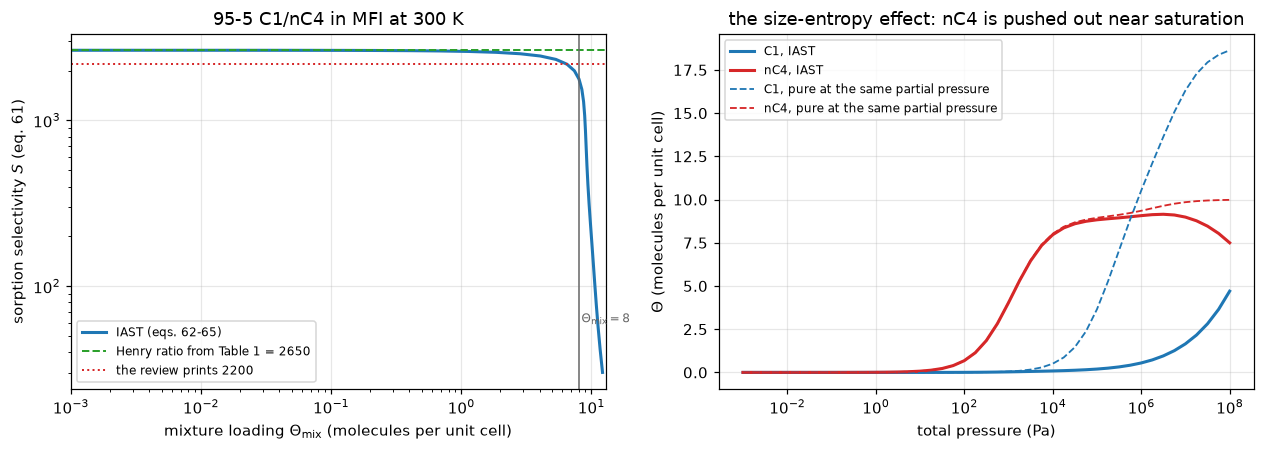
The nC4 loading peaks at 9.149 molecules per unit cell at a total
pressure of 3.2e+06 Pa and then DECLINES as the pressure rises further,
reaching 7.499 at 1e+08 Pa while C1 climbs from 0.956 to 4.701.
The review describes exactly that ('increasing the total system pressure
beyond 5 MPa leads to a decline in the loading of nC4!'), and it is the
whole reason the multicomponent Langmuir cannot be used: no Langmuir
isotherm has a non-monotonic component loading.
2. The hexane isomers sorb the other way round
The same machinery on Table 2’s parameters at 362 K. Here the review states a threshold: separation works when the upstream mixture loading exceeds 4 molecules per unit cell, “at 362 K this corresponds to a total upstream pressure in excess of 1 kPa”.
def hex_sorption(nc6, mp3):
    """Equimolar nC6/3MP sorption: the pressure at Theta_mix = 4 (a direct root on
    [1 Pa, 1 MPa]; Theta_mix increases with pressure) and Theta_mix at 1 kPa."""
    hm = IAST([nc6, mp3])
    f = lambda lp: hm.forward(0.5 * (10 ** lp) * np.ones(2))[0].sum() - 4.0
    if not f(0) < 0 < f(6):
        raise ValueError("Theta_mix = 4 is not bracketed by 1 Pa and 1 MPa")
    p4 = 10 ** brentq(f, 0, 6, xtol=1e-12)
    th1 = float(hm.forward(0.5 * PRINTED["hex_P_theta4"] * np.ones(2))[0].sum())
    return hm, p4, th1


hex_mix, P_TH4, TH_AT_1KPA = hex_sorption(NC6, MP3)
Ph = np.logspace(0, 6, 55)
Thh = hex_mix.forward(0.5 * Ph[:, None] * np.ones(2))
print(f"IAST puts Theta_mix = 4 at a total pressure of {P_TH4:.1f} Pa "
      f"({P_TH4/1e3:.3f} kPa).")
print(f"The review states 'in excess of {PRINTED['hex_P_theta4']/1e3:.0f} kPa'; at "
      f"exactly that pressure IAST gives Theta_mix = {TH_AT_1KPA:.2f}.")
print("The review's statement is therefore CORRECT but loose by a factor of "
      f"{PRINTED['hex_P_theta4']/P_TH4:.1f};")
print("it is a sufficient condition, not the threshold, and is scored as such.\n")
print(f"{'P_total/kPa':>12}{'Theta_nC6':>11}{'Theta_3MP':>11}{'Theta_mix':>11}"
      f"{'S (nC6/3MP)':>13}")
for P in (0.1e3, 0.5e3, 1e3, 4e3, 15e3, 66e3):
    T = hex_mix.forward(0.5 * P * np.ones(2))[0]
    print(f"{P/1e3:12.2f}{T[0]:11.4f}{T[1]:11.4f}{T.sum():11.4f}{T[0]/T[1]:13.3f}")
print("\nBelow Theta_mix = 4 the two isomers sorb almost equally; above it the")
print("branched one is squeezed out of the channel interiors. That is the")
print("configurational-entropy effect the separation is built on, and it is")
print("produced here by IAST from the pure-component fits alone.")
IAST puts Theta_mix = 4 at a total pressure of 156.1 Pa (0.156 kPa).
The review states 'in excess of 1 kPa'; at exactly that pressure IAST gives Theta_mix = 5.36.
The review's statement is therefore CORRECT but loose by a factor of 6.4;
it is a sufficient condition, not the threshold, and is scored as such.
P_total/kPa Theta_nC6 Theta_3MP Theta_mix S (nC6/3MP)
0.10 2.2338 1.4417 3.6754 1.549
0.50 3.2957 1.5191 4.8148 2.169
1.00 3.9584 1.4004 5.3588 2.827
4.00 5.6198 0.9809 6.6007 5.729
15.00 6.8274 0.6421 7.4695 10.633
66.00 7.3775 0.4293 7.8069 17.184
Below Theta_mix = 4 the two isomers sorb almost equally; above it the
branched one is squeezed out of the channel interiors. That is the
configurational-entropy effect the separation is built on, and it is
produced here by IAST from the pure-component fits alone.3. The membrane, and where the 1.73 goes
Now eqs. (57)–(59). Four runs: the 95–5 and 50–50 mixtures, each with the exchange coefficients from eq. (43) and with \(\eth_{ij}\to\infty\), each solved directly from the linear initial profile. Every selectivity below is independent of the membrane thickness, the framework density and the absolute size of the diffusivities.
FEEDS = {"95-5": np.array([P_C1, P_NC4]), "50-50": np.array([50e3, 50e3])}
NZ_STEADY = 40
SP_PURE = A47_VAL["sp_pure"]
STEADY_LOG = []          # (case, newton iterations, flux spread, continued)


def steady_runs(force_Dij=None, n_z=NZ_STEADY, steady_kw=None, **kw):
    """The four production solves; ``kw``, ``force_Dij`` and ``steady_kw``
    inject break-table defects."""
    out = {}
    for feed, p0 in FEEDS.items():
        for mode in ("vignes", "inf"):
            m = membrane(n_z=n_z, Dij=force_Dij or mode, **kw)
            Th_m, J = m.steady(p0, **(steady_kw or {}))
            STEADY_LOG.append((f"{feed} {mode}", m.newton_its, m.flux_spread, m.continued))
            out[(feed, mode)] = (m, Th_m, J, selectivity(J, p0))
    return out


RUNS = steady_runs()
print(f"{'feed':>7}{'exchange':>26}{'Newton':>8}{'route':>8}{'flux spread':>13}"
      f"{'S_P':>10}{'printed':>10}{'dev':>9}")
for (feed, mode), (m, _, J, s_p) in RUNS.items():
    lab = "finite, eq. (43)" if mode == "vignes" else "infinite, eq. (47)"
    key = f"mix_SP_{feed.replace('-', '')}_{'finite' if mode=='vignes' else 'inf'}"
    pr = PRINTED[key]
    route = "cont." if m.continued else "direct"
    print(f"{feed:>7}{lab:>26}{m.newton_its:8d}{route:>8}{'(here ' + format(m.flux_spread, '.0e') + ')':>16}"
          f"{s_p:10.2f}{pr:10.1f}{(s_p/pr-1)*100:8.2f}%")
N_CONTINUED = sum(int(m.continued) for (m, _, _, _) in RUNS.values())

SP_955 = RUNS[("95-5", "vignes")][3]
SP_955_INF = RUNS[("95-5", "inf")][3]
SP_5050 = RUNS[("50-50", "vignes")][3]
SP_5050_INF = RUNS[("50-50", "inf")][3]
print(f"\nA4.7's stored pure-component expectation is S_P = {SP_PURE}, and eq. (60)")
print(f"on its stored fluxes gives {(FLUX_NC4/FLUX_C1)/(P_NC4/P_C1):.3f}: arithmetic on two "
      "printed")
print("numbers, which tests the transcription and nothing else.")
print(f"The mixture value is {SP_955/SP_PURE:.0f}x larger, and removing the "
      "sorbate-sorbate")
print(f"friction alone takes it back down by a factor of "
      f"{SP_955/SP_955_INF:.1f}, to {SP_955_INF:.1f}.")
feed exchange Newton route flux spread S_P printed dev
95-5 finite, eq. (43) 8 direct (here 1e-13) 488.23 487.0 0.25%
95-5 infinite, eq. (47) 7 direct (here 2e-13) 12.36 12.3 0.53%
50-50 finite, eq. (43) 9 direct (here 1e-13) 202.93 202.0 0.46%
50-50 infinite, eq. (47) 7 direct (here 1e-13) 5.44 5.4 0.74%
A4.7's stored pure-component expectation is S_P = 1.73, and eq. (60)
on its stored fluxes gives 1.732: arithmetic on two printed
numbers, which tests the transcription and nothing else.
The mixture value is 282x larger, and removing the sorbate-sorbate
friction alone takes it back down by a factor of 39.5, to 12.4.The absolute fluxes need a membrane thickness, which the review never prints. A4.7 obtained \(\delta\approx 40\ \mu\)m by inverting each of the two single-component steady fluxes with the only MFI density the review prints, 1800 kg m⁻³ from the caption of Fig. 40. It is reconstructed here from the same stored rows and used to put the four mixture fluxes into mmol m⁻² s⁻¹.
What that comparison tests, and what it cannot, stated before the numbers. It is not an out-of-sample test of A4.7’s \(\delta\) on the \(1/\delta\) power: \(\delta\) cancels identically. Substituting the reconstruction \(\delta=\rho_{\rm uc}\eth_{\rm C1}\psi_{\rm C1}(95\ {\rm kPa})/(N_A N_{\rm C1})\) into the conversion \(N_i=\rho_{\rm uc}J_i/(N_A\delta)\) leaves
\[N_i \;=\; N_{\rm C1}^{\rm stored}\,\frac{J_i}{\eth_{\rm C1}\,\psi_{\rm C1}(95\ {\rm kPa})},\]
with no \(\delta\), no \(\rho_{\rm MFI}\), no unit-cell mass and no Avogadro constant left in it. A four-fold error in the framework density would leave all four “absolute” fluxes unchanged, and the cell below demonstrates that rather than asserting it. So this comparison is the \(\delta\)-free flux-ratio comparison printed below it, rescaled by the stored 34: the two deviations differ only by the \(n=1\) solver’s discretisation error against the analytic \(\psi\), and both are printed so that the coincidence is visible.
What survives is still worth having, and it is about the physics rather than the thickness: the pure C1 flux is guaranteed to come out at the stored 34 (that is what \(\delta\) was fitted to) and the pure nC4 flux carries A4.7’s flux-ratio deviation and nothing more, whereas the four mixture fluxes run through IAST, a matrix \([\Gamma]\) and finite \(\eth_{ij}\), none of which entered the reconstruction, and none of which is guaranteed to land anywhere. The one quantity on this page that does carry \(\delta\) is the transient peak time, taken up in the next section.
NA = 6.02214076e23
M_CELL = (96 * 28.0855 + 192 * 15.999) / NA * 1e-3      # kg per Si96O192 unit cell


def thickness(rho, flux, D, iso_, p):
    """`A4.7`'s inversion of a single-component flux for the membrane thickness (m)."""
    return float(rho / M_CELL * D * iso_.psi(p) / NA / (flux * 1e-3))


RHO_UC = A47_VAL["rho_MFI"] / M_CELL                    # unit cells per m3
DELTA = thickness(A47_VAL["rho_MFI"], FLUX_C1, D_C1, C1, P_C1)
DELTA_NC4 = thickness(A47_VAL["rho_MFI"], FLUX_NC4, D_NC4, NC4, P_NC4)
print("A4.7's reconstruction, recomputed from the same stored rows:")
print(f"   from the stored C1 flux  : {DELTA*1e6:.3f} um")
print(f"   from the stored nC4 flux : {DELTA_NC4*1e6:.3f} um   "
      f"({abs(DELTA_NC4/DELTA-1)*100:.2f} % apart: this IS the flux-ratio check")
print("     inverted, not a second one)\n")


def mmol(J, L=1.0, rho_uc=RHO_UC, delta=DELTA):
    """Solver flux -> mmol m^-2 s^-1. ``L`` is the thickness the grid was built
    on: the thickness-free runs use L = 1 and the dimensional ones L = DELTA."""
    return rho_uc * np.asarray(J) * (L / delta) / NA * 1e3


FLUX_KEYS = (("95-5", "vignes", 0, "mix_N_C1_finite"), ("95-5", "vignes", 1, "mix_N_nC4_finite"),
             ("95-5", "inf", 0, "mix_N_C1_inf"), ("95-5", "inf", 1, "mix_N_nC4_inf"))


def flux_rows(runs):
    out = []
    for feed, mode, comp, key in FLUX_KEYS:
        v = float(mmol(runs[(feed, mode)][2].mean(0))[comp])
        lab = (f"{'C1' if comp == 0 else 'nC4'}, {feed}, "
               f"{'finite' if mode == 'vignes' else 'infinite'} Dij")
        out.append((lab, PRINTED[key], v))
    return out


FLUX_ROWS = flux_rows(RUNS)
print(f"{'case':>34}{'computed':>11}{'printed':>10}{'dev':>9}")
for lab, pr, v in FLUX_ROWS:
    print(f"{lab:>34}{v:11.4f}{pr:10.2f}{(v/pr-1)*100:8.2f}%")
FLUX_WORST = max(abs(v / p - 1) for _, p, v in FLUX_ROWS)
print(f"\nWorst of the four mixture fluxes: {FLUX_WORST*100:.2f} %, against printed")
print("values carrying two or three significant figures. What that does NOT test")
print("is delta, and the demonstration is below.")

print("\nDELTA, rho_MFI, THE UNIT-CELL MASS AND N_A ALL CANCEL. Swing the framework")
print("density over a factor of four, which moves the reconstructed thickness")
print("over the same factor, and the four fluxes do not move:")
print(f"\n{'rho_MFI / kg m^-3':>19}{'delta / um':>13}{'N_C1 (finite)':>18}"
      f"{'N_nC4 (finite)':>18}{'worst of 4':>12}")
J_FIN = RUNS[("95-5", "vignes")][2].mean(0)
J_INF = RUNS[("95-5", "inf")][2].mean(0)
BASE4 = np.concatenate([mmol(J_FIN), mmol(J_INF)])
RHO_SWING = 0.0
for rho in (A47_VAL["rho_MFI"], 1200.0, 3600.0, 900.0):
    dl = thickness(rho, FLUX_C1, D_C1, C1, P_C1)
    four = np.concatenate([mmol(J, rho_uc=rho / M_CELL, delta=dl) for J in (J_FIN, J_INF)])
    RHO_SWING = max(RHO_SWING, float(np.max(np.abs(four / BASE4 - 1))))
    print(f"{rho:19.0f}{dl*1e6:13.4f}{four[0]:18.12f}{four[1]:18.12f}"
          f"   (here {np.max(np.abs(four - BASE4)):.0e})")


def cancellation_residual(rho_conversion=A47_VAL["rho_MFI"]):
    """The conversion against its closed form N_i = 34 J_i/(D_C1 psi_C1).
    ``rho_conversion`` other than the density delta was built from is the defect."""
    closed = FLUX_C1 * np.asarray(J_FIN) / (D_C1 * C1.psi(P_C1))
    return float(np.max(np.abs(closed / mmol(J_FIN, rho_uc=rho_conversion / M_CELL) - 1)))


DELTA_CANCELS = cancellation_residual()
print(f"\n   because the conversion collapses algebraically to "
      f"N_i = {FLUX_C1:g} J_i / (D_C1 psi_C1),")
print(f"   verified against the code path above to (here {DELTA_CANCELS:.0e}), round-off.")
print("   So the four-flux comparison is the delta-free flux-RATIO comparison")
print("   below, multiplied by the stored 34. It is a real test of the MIXTURE")
print("   physics (IAST, [Gamma] and finite Dij all enter J_i) and no test at")
print("   all of the membrane thickness. Kept and labelled rather than deleted,")
print("   because deleting it would hide that the two rows are one check.")


def pure_fluxes(n_z=120, **kw):
    """The two single-component membranes (n = 1), thickness-free."""
    jc1 = Membrane([C1], [C1.Th_sat], [D_C1], n_z=n_z, **kw).steady(np.array([P_C1]))[1]
    jc4 = Membrane([NC4], [NC4.Th_sat], [D_NC4], n_z=n_z, **kw).steady(np.array([P_NC4]))[1]
    return float(jc1.mean(0)[0]), float(jc4.mean(0)[0])


def ratio_free(runs, jp):
    JM = runs[("95-5", "vignes")][2].mean(0)
    r_c1, r_nc4 = float(JM[0]) / jp[0], float(JM[1]) / jp[1]
    worst = max(abs(r_c1 / (PRINTED["mix_N_C1_finite"] / FLUX_C1) - 1),
                abs(r_nc4 / (PRINTED["mix_N_nC4_finite"] / FLUX_NC4) - 1))
    return r_c1, r_nc4, worst


JP = pure_fluxes()
R_C1, R_NC4, RATIO_FREE_WORST = ratio_free(RUNS, JP)
print(f"\nThe same statement with delta removed entirely, as flux ratios:")
print(f"   N_C1(mixture)/N_C1(pure)  : computed {R_C1:.5f}   printed "
      f"{PRINTED['mix_N_C1_finite']/FLUX_C1:.5f}   "
      f"({(R_C1/(PRINTED['mix_N_C1_finite']/FLUX_C1)-1)*100:+.2f} %)")
print(f"   N_nC4(mixture)/N_nC4(pure): computed {R_NC4:.5f}   printed "
      f"{PRINTED['mix_N_nC4_finite']/FLUX_NC4:.5f}   "
      f"({(R_NC4/(PRINTED['mix_N_nC4_finite']/FLUX_NC4)-1)*100:+.2f} %)")
print(f"   Methane's flux collapses by a factor of {1/R_C1:.0f} in the mixture while butane's")
print(f"   is essentially unchanged ({(R_NC4-1)*100:+.1f} %). That asymmetry is the whole effect.")
print(f"\n   And there is the coincidence, in the open: the four-flux worst")
print(f"   deviation is {FLUX_WORST:.7f} and this delta-free one is {RATIO_FREE_WORST:.7f}. They")
print(f"   differ by {abs(FLUX_WORST-RATIO_FREE_WORST):.1e} in absolute terms, which is the "
      "n = 1 SOLVER")
print("   against the analytic psi and nothing else: they are the same check")
print("   reported twice, and both are kept.")
ANA = (D_C1 * C1.psi(P_C1), D_NC4 * NC4.psi(P_NC4))
COLLAPSE_1 = max(abs(JP[0] / ANA[0] - 1), abs(JP[1] / ANA[1] - 1))
print(f"\n   (eq. 45 run with n = 1 against the closed-form eq. (12) integral: {COLLAPSE_1:.1e})")
A4.7's reconstruction, recomputed from the same stored rows:
from the stored C1 flux : 39.967 um
from the stored nC4 flux : 40.036 um (0.17 % apart: this IS the flux-ratio check
inverted, not a second one)
case computed printed dev
C1, 95-5, finite Dij 0.1205 0.12 0.41%
nC4, 95-5, finite Dij 3.0961 3.09 0.20%
C1, 95-5, infinite Dij 4.7186 4.72 -0.03%
nC4, 95-5, infinite Dij 3.0708 3.06 0.35%
Worst of the four mixture fluxes: 0.41 %, against printed
values carrying two or three significant figures. What that does NOT test
is delta, and the demonstration is below.
DELTA, rho_MFI, THE UNIT-CELL MASS AND N_A ALL CANCEL. Swing the framework
density over a factor of four, which moves the reconstructed thickness
over the same factor, and the four fluxes do not move:
rho_MFI / kg m^-3 delta / um N_C1 (finite) N_nC4 (finite) worst of 4
1800 39.9671 0.120487871010 3.096103685318 (here 0e+00)
1200 26.6447 0.120487871010 3.096103685318 (here 9e-16)
3600 79.9341 0.120487871010 3.096103685318 (here 0e+00)
900 19.9835 0.120487871010 3.096103685318 (here 0e+00)
because the conversion collapses algebraically to N_i = 34 J_i / (D_C1 psi_C1),
verified against the code path above to (here 2e-16), round-off.
So the four-flux comparison is the delta-free flux-RATIO comparison
below, multiplied by the stored 34. It is a real test of the MIXTURE
physics (IAST, [Gamma] and finite Dij all enter J_i) and no test at
all of the membrane thickness. Kept and labelled rather than deleted,
because deleting it would hide that the two rows are one check.
The same statement with delta removed entirely, as flux ratios:
N_C1(mixture)/N_C1(pure) : computed 0.00354 printed 0.00353 (+0.41 %)
N_nC4(mixture)/N_nC4(pure): computed 0.99714 printed 0.99677 (+0.04 %)
Methane's flux collapses by a factor of 282 in the mixture while butane's
is essentially unchanged (-0.3 %). That asymmetry is the whole effect.
And there is the coincidence, in the open: the four-flux worst
deviation is 0.0040656 and this delta-free one is 0.0040675. They
differ by 1.9e-06 in absolute terms, which is the n = 1 SOLVER
against the analytic psi and nothing else: they are the same check
reported twice, and both are kept.
(eq. 45 run with n = 1 against the closed-form eq. (12) integral: 1.1e-04)The transient, and a peak that arrives before the butane does
The review reports that during the initial transience the methane flux overshoots (0.44 mmol m⁻² s⁻¹ at t = 0.73 s with finite exchange, 17.2 with \(\eth_{ij}\to\infty\)), because methane fills the membrane first and is then displaced by the more strongly adsorbed butane.
The peak time is the only quantity on this page that carries \(\delta\) at all, and it carries it as \(\delta^2\) where a steady flux carries it as \(1/\delta\). The four mixture fluxes above look like a second, independent handle on the reconstruction and are not one, so this section is where A4.7’s \(\approx 40\ \mu\)m is tested, and it is the only place it is tested.
The transient has to be resolved in space, and it is a different resolution problem from the steady one. The grid study in Validation refines the steady selectivity, where the loading profile is smooth. The transient carries a butane front, and its steepness is set by the site-A affinity at the upstream face, printed below. Refining the steady solution says nothing about it, so the grid is refined here, under the transient, before any number from it is reported.
# Output times: a log sweep for the whole transient, plus a dense linear window
# through the peak so that its POSITION is not set by the output grid spacing.
T_LOG = np.logspace(-3, 3.3, 48)
t_out = np.unique(np.concatenate([T_LOG, np.linspace(0.45, 1.15, 15)]))
t_pk = t_out[t_out <= 3.0]          # far enough past the peak to bracket it
NZ_PROD = 120                       # production grid, justified by the study below


TRANSIENT_STATS = []      # (cutbacks, accepted steps that needed a guard) of every run


def run_transient(n_z, mode, dt_frac, tt, maxit=40):
    m = membrane(n_z=n_z, Dij=mode, delta=DELTA)
    rec = m.transient(np.array([P_C1, P_NC4]), tt, dt_frac=dt_frac, maxit=maxit)
    TRANSIENT_STATS.append((m.cutbacks, m.guard_accepted))
    N = np.array([mmol(r[2][-1], DELTA) for r in rec])
    return m, rec, N


def front_jumps(m, rec):
    """Largest cell-to-cell jump in the nC4 loading over its upstream face value,
    at every output time."""
    th_face = float(m.load(np.array([[P_C1, P_NC4]]))[0][1])
    return [(t, float(np.max(np.abs(np.diff(Th_[:, 1]))) / th_face)) for t, Th_, _ in rec]


print("WHY THE STEADY GRID STUDY DOES NOT COVER THIS.\n")
for nm, iso_, p0_ in (("C1 ", C1, P_C1), ("nC4", NC4, P_NC4)):
    bp = iso_.bA * p0_
    print(f"   {nm}: site-A affinity at the upstream face, b_A p = {bp:8.2f}"
          f"   -> that site is {100*bp/(1+bp):5.1f} % full")
print("   Both are essentially empty at the swept face. nC4 is the problem: a")
print("   site that is nearly saturated at one face and empty at the other has")
print("   an almost rectangular isotherm, and an almost rectangular isotherm")
print("   makes a SELF-SHARPENING front while it fills. The steady profile has")
print("   no such front; the transient does, and it has to be resolved.")

TRANS = {}
for mode in ("vignes", "inf"):
    m, rec, N = run_transient(NZ_PROD, mode, 0.05, t_out)
    TRANS[mode] = (m, N, rec)
    print(f"\n   {mode:7s} at n_z = {NZ_PROD}: {m.nsteps} steps, at most "
          f"{m.maxinner} inner iterations, {m.cutbacks} cutbacks, "
          f"{m.guard_accepted} accepted steps that needed a guard")
PEAKS = {mode: locate_peak(t_out, TRANS[mode][1][:, 0]) for mode in ("vignes", "inf")}

JUMPS = front_jumps(TRANS["vignes"][0], TRANS["vignes"][2])
T_WORST, FRONT_T = max(JUMPS, key=lambda r: r[1])
FRONT_PK = JUMPS[PEAKS["vignes"][2]][1]
FRONT_S = JUMPS[-1][1]
print(f"\n   Measured on the n_z = {NZ_PROD} run, as the largest cell-to-cell jump in")
print(f"   the nC4 loading over the upstream face value:")
print(f"      worst over the whole transient (t = {T_WORST:.3g} s) : {FRONT_T*100:6.2f} %")
print(f"      at the peak time                            : {FRONT_PK*100:6.2f} %")
print(f"      at steady state                             : {FRONT_S*100:6.2f} %")
print(f"   {FRONT_T/FRONT_S:.0f}x at its worst. Early on one cell carries most of the whole")
print("   loading step, because the front starts AT the face; by the time of the")
print("   peak it has spread. The steady profile never has such a cell.")
print("   That is the mechanism; the evidence is the grid study below.")
WHY THE STEADY GRID STUDY DOES NOT COVER THIS.
C1 : site-A affinity at the upstream face, b_A p = 0.46 -> that site is 31.6 % full
nC4: site-A affinity at the upstream face, b_A p = 81.50 -> that site is 98.8 % full
Both are essentially empty at the swept face. nC4 is the problem: a
site that is nearly saturated at one face and empty at the other has
an almost rectangular isotherm, and an almost rectangular isotherm
makes a SELF-SHARPENING front while it fills. The steady profile has
no such front; the transient does, and it has to be resolved.
vignes at n_z = 120: 437 steps, at most 20 inner iterations, 0 cutbacks, 0 accepted steps that needed a guard
inf at n_z = 120: 437 steps, at most 31 inner iterations, 0 cutbacks, 0 accepted steps that needed a guard
Measured on the n_z = 120 run, as the largest cell-to-cell jump in
the nC4 loading over the upstream face value:
worst over the whole transient (t = 0.001 s) : 76.61 %
at the peak time : 5.83 %
at steady state : 3.61 %
21x at its worst. Early on one cell carries most of the whole
loading step, because the front starts AT the face; by the time of the
peak it has spread. The steady profile never has such a cell.
That is the mechanism; the evidence is the grid study below.print("GRID STUDY UNDER THE TRANSIENT. Only n_z changes; t_out, dt_frac = 0.05\n"
"and locate_peak are the ones used for the production run.\n")
GRID_T, FRONT_GRID = {}, {}
for mode in ("vignes", "inf"):
lvls = (30, 60, 240) if mode == "vignes" else (30, 60)
rows_ = []
for nz in lvls:
m_, rec_, N = run_transient(nz, mode, 0.05, t_pk)
tp, yp, _ = locate_peak(t_pk, N[:, 0])
rows_.append((nz, tp, yp))
if mode == "vignes" and nz == 30:
j30 = front_jumps(m_, rec_)
FRONT_GRID[30] = max(j for _, j in j30) / j30[-1][1]
rows_.append((NZ_PROD, PEAKS[mode][0], PEAKS[mode][1])) # the production run
GRID_T[mode] = sorted(rows_)
for mode, kf, kt in (("vignes", "mix_peak_C1_finite", "mix_peak_t_finite"),
("inf", "mix_peak_C1_inf", None)):
lab = "finite Dij (eq. 43)" if mode == "vignes" else "Dij -> infinity (eq. 47)"
print(f" {lab}")
print(f" {'n_z':>6}{'peak N_C1':>12}{'vs printed':>12}{'t_peak/s':>11}{'vs printed':>12}")
for nz, tp, yp in GRID_T[mode]:
tcol = (f"{(tp/PRINTED[kt]-1)*100:+11.2f}%" if kt else f"{'-':>12}")
star = " <-- production" if nz == NZ_PROD else ""
print(f" {nz:6d}{yp:12.4f}{(yp/PRINTED[kf]-1)*100:+11.2f}%{tp:11.4f}{tcol}{star}")
print()
gv = {nz: (tp, yp) for nz, tp, yp in GRID_T["vignes"]}
gi = {nz: (tp, yp) for nz, tp, yp in GRID_T["inf"]}
def grid_order(a, b, c):
"""Observed order from three levels refined by 2, from successive differences."""
return float(np.log2(abs(a - b) / abs(b - c)))
def richardson(fine, coarse, p):
return fine + (fine - coarse) / (2 ** p - 1)
T_ORDER = grid_order(gv[30][0], gv[60][0], gv[NZ_PROD][0])
T_ORDER2 = grid_order(gv[60][0], gv[NZ_PROD][0], gv[240][0])
T_RICH = richardson(gv[240][0], gv[NZ_PROD][0], T_ORDER2)
T_GRID_ERR = abs(gv[NZ_PROD][0] / T_RICH - 1)
# the finest difference against the inner-iteration tolerance it is measured through
T_DIFF_OVER_TOL = abs(gv[NZ_PROD][0] - gv[240][0]) / (1e-11 * gv[240][0])
print(f" Observed order on t_peak: {T_ORDER:.2f} (30/60/120), then {T_ORDER2:.2f} "
"(60/120/240).")
print(" The scheme is second order in space, so the first value is pre-asymptotic;")
print(f" the second is in range. Richardson from the last pair extrapolates to {T_RICH:.4f} s,")
print(f" so the production n_z = {NZ_PROD} carries {T_GRID_ERR*100:.2f} % of spatial error "
"on the peak")
print(f" time, {abs(gv[NZ_PROD][0]/PRINTED['mix_peak_t_finite']-1)/T_GRID_ERR:.0f}x smaller "
"than its disagreement with the review, so it does not explain it.")
print(f"\n THE COARSE GRID FLATTERS BOTH NUMBERS, IN OPPOSITE DIRECTIONS. At")
print(f" n_z = 30 the peak time is {gv[30][0]:.4f} s, "
f"{(gv[30][0]/PRINTED['mix_peak_t_finite']-1)*100:+.1f} % from the printed "
f"{PRINTED['mix_peak_t_finite']}, and the")
print(f" peak height {gv[30][1]:.4f}, {(gv[30][1]/PRINTED['mix_peak_C1_finite']-1)*100:+.1f} %"
f" from the printed {PRINTED['mix_peak_C1_finite']}. Refined, the time moves")
print(f" AWAY to {(gv[NZ_PROD][0]/PRINTED['mix_peak_t_finite']-1)*100:+.1f} % and the height "
f"CROSSES to {(gv[NZ_PROD][1]/PRINTED['mix_peak_C1_finite']-1)*100:+.1f} %. The dominant")
print(f" error on the coarse grid is spatial: refining 30 -> {NZ_PROD} cells moves the height")
print(f" by {(gv[NZ_PROD][1]/gv[30][1]-1)*100:+.1f} %, more than the step refinement below does.")GRID STUDY UNDER THE TRANSIENT. Only n_z changes; t_out, dt_frac = 0.05
and locate_peak are the ones used for the production run.
finite Dij (eq. 43)
n_z peak N_C1 vs printed t_peak/s vs printed
30 0.4334 -1.51% 0.7241 -0.81%
60 0.4442 +0.95% 0.6685 -8.43%
120 0.4452 +1.19% 0.6583 -9.82% <-- production
240 0.4449 +1.11% 0.6558 -10.16%
Dij -> infinity (eq. 47)
n_z peak N_C1 vs printed t_peak/s vs printed
30 16.6048 -3.46% 0.7929 -
60 17.3107 +0.64% 0.7030 -
120 17.5068 +1.78% 0.6756 - <-- production
Observed order on t_peak: 2.46 (30/60/120), then 2.01 (60/120/240).
The scheme is second order in space, so the first value is pre-asymptotic;
the second is in range. Richardson from the last pair extrapolates to 0.6550 s,
so the production n_z = 120 carries 0.51 % of spatial error on the peak
time, 19x smaller than its disagreement with the review, so it does not explain it.
THE COARSE GRID FLATTERS BOTH NUMBERS, IN OPPOSITE DIRECTIONS. At
n_z = 30 the peak time is 0.7241 s, -0.8 % from the printed 0.73, and the
peak height 0.4334, -1.5 % from the printed 0.44. Refined, the time moves
AWAY to -9.8 % and the height CROSSES to +1.2 %. The dominant
error on the coarse grid is spatial: refining 30 -> 120 cells moves the height
by +2.7 %, more than the step refinement below does.print("TIME-STEP STUDY, AT THE PRODUCTION GRID. Three levels, not two.\n")
i_pk = PEAKS["vignes"][2]
GRID_SPACING = t_out[i_pk + 1] / t_out[i_pk] - 1
DT_ROWS = [(0.05, PEAKS["vignes"][0], PEAKS["vignes"][1])]
for dtf in (0.025, 0.0125):
_, _, N_f = run_transient(NZ_PROD, "vignes", dtf, t_pk)
DT_ROWS.append((dtf,) + locate_peak(t_pk, N_f[:, 0])[:2])
print(f" output grid spacing at the peak: {GRID_SPACING*100:.1f} %\n")
print(f" {'dt_frac':>9}{'peak N_C1':>12}{'vs printed':>12}{'t_peak/s':>11}{'vs printed':>12}")
for dtf, tp, yp in DT_ROWS:
star = " <-- production" if dtf == 0.05 else ""
print(f" {dtf:9.4f}{yp:12.4f}"
f"{(yp/PRINTED['mix_peak_C1_finite']-1)*100:+11.2f}%{tp:11.4f}"
f"{(tp/PRINTED['mix_peak_t_finite']-1)*100:+11.2f}%{star}")
def dt_numbers(r0, r1, r2):
"""Shifts from the first halving and successive-difference ratios."""
return dict(peak_height_dt_halved_shift=abs(r1[2] / r0[2] - 1),
peak_time_dt_halved_shift=abs(r1[1] / r0[1] - 1),
dt_ratio_height=abs(r0[2] - r1[2]) / abs(r1[2] - r2[2]),
dt_ratio_time=abs(r0[1] - r1[1]) / abs(r1[1] - r2[1]))
DTN = dt_numbers(*DT_ROWS)
DT_PEAK_SHIFT, DT_TIME_SHIFT = DTN["peak_height_dt_halved_shift"], DTN["peak_time_dt_halved_shift"]
print(f"\n successive-difference ratios: height {DTN['dt_ratio_height']:.2f}, "
f"time {DTN['dt_ratio_time']:.2f}. The height")
print(f" is consistent with the first order backward Euler has; the TIME is not,")
print(f" so no extrapolation in dt is offered for it, only the direction, which")
print(" is unambiguous. BOTH refinements push the same way: the height further")
print(f" ABOVE the printed {PRINTED['mix_peak_C1_finite']} and the time further BELOW "
f"the printed {PRINTED['mix_peak_t_finite']} s.")
print(f" The reported values are the coarsest of the three, dt_frac = 0.05, so")
print(" the disagreement below is if anything understated.")
def delta_shift(t_peak):
"""Relative change of delta that moves a peak time to the printed one (t ~ delta^2)."""
return float(np.sqrt(PRINTED["mix_peak_t_finite"] / t_peak) - 1)
T_PEAK_DEV = PEAKS["vignes"][0] / PRINTED["mix_peak_t_finite"] - 1
DELTA_FOR_PEAK = delta_shift(PEAKS["vignes"][0])
DELTA_FOR_PEAK_FINE = delta_shift(DT_ROWS[-1][1])
print(f"\nWHAT THAT DOES TO A4.7'S RECONSTRUCTED THICKNESS. Converged, the peak")
print(f"time is {PEAKS['vignes'][0]:.4f} s against the printed "
f"{PRINTED['mix_peak_t_finite']} s, {T_PEAK_DEV*100:+.1f} %. Since")
print(f"t_peak scales as delta^2, closing that gap needs delta "
f"{DELTA_FOR_PEAK*100:+.1f} %, i.e.")
print(f"{DELTA*1e6:.1f} um -> {DELTA*(1+DELTA_FOR_PEAK)*1e6:.1f} um; at the finest step tried it "
f"is {DELTA_FOR_PEAK_FINE*100:+.1f} %. delta was")
print(f"inverted from a flux printed to two figures, and half a unit on {FLUX_C1:g} is only")
print(f"{0.5/FLUX_C1*100:.1f} %, so rounding does not cover it either.")
print("\nTHIS IS AN OPEN TENSION and is reported as one. The four printed fluxes")
print("do not contain delta, so nothing about them constrains it. It sits in some")
print("combination of:")
print(f" * rho_MFI = {A47_VAL['rho_MFI']:g} kg m^-3, read off a figure caption and")
print(" constrained by nothing else on this page or on A4.7; delta scales")
print(" with it directly, so a 5 % error there is a 5 % error here;")
print(" * the Si96O192 unit-cell mass, hard-coded here from atomic weights and")
print(" traceable to nothing printed in the review;")
print(f" * the printed {FLUX_C1:g} mmol m^-2 s^-1 that delta was inverted from, two figures;")
print(" * the review's transient itself, which may not be the calculation")
print(" reproduced here: it prints no delta, no grid and no time step.")
print("Nothing on this page decides between them, and nothing was adjusted.")TIME-STEP STUDY, AT THE PRODUCTION GRID. Three levels, not two.
output grid spacing at the peak: 7.2 %
dt_frac peak N_C1 vs printed t_peak/s vs printed
0.0500 0.4452 +1.19% 0.6583 -9.82% <-- production
0.0250 0.4487 +1.98% 0.6507 -10.86%
0.0125 0.4506 +2.41% 0.6448 -11.68%
successive-difference ratios: height 1.87, time 1.28. The height
is consistent with the first order backward Euler has; the TIME is not,
so no extrapolation in dt is offered for it, only the direction, which
is unambiguous. BOTH refinements push the same way: the height further
ABOVE the printed 0.44 and the time further BELOW the printed 0.73 s.
The reported values are the coarsest of the three, dt_frac = 0.05, so
the disagreement below is if anything understated.
WHAT THAT DOES TO A4.7'S RECONSTRUCTED THICKNESS. Converged, the peak
time is 0.6583 s against the printed 0.73 s, -9.8 %. Since
t_peak scales as delta^2, closing that gap needs delta +5.3 %, i.e.
40.0 um -> 42.1 um; at the finest step tried it is +6.4 %. delta was
inverted from a flux printed to two figures, and half a unit on 34 is only
1.5 %, so rounding does not cover it either.
THIS IS AN OPEN TENSION and is reported as one. The four printed fluxes
do not contain delta, so nothing about them constrains it. It sits in some
combination of:
* rho_MFI = 1800 kg m^-3, read off a figure caption and
constrained by nothing else on this page or on A4.7; delta scales
with it directly, so a 5 % error there is a 5 % error here;
* the Si96O192 unit-cell mass, hard-coded here from atomic weights and
traceable to nothing printed in the review;
* the printed 34 mmol m^-2 s^-1 that delta was inverted from, two figures;
* the review's transient itself, which may not be the calculation
reproduced here: it prints no delta, no grid and no time step.
Nothing on this page decides between them, and nothing was adjusted.fig, axes = plt.subplots(1, 2, figsize=(11.6, 4.2))
for ax, mode, ttl in ((axes[0], "vignes", r"finite $\eth_{ij}$ (eq. 43)"),
(axes[1], "inf", r"$\eth_{ij}\to\infty$ (eq. 47)")):
N = TRANS[mode][1]
ax.loglog(t_out, N[:, 0], lw=2.0, color="tab:blue", label="C1")
ax.loglog(t_out, N[:, 1], lw=2.0, color="tab:red", label="nC4")
tp, yp = PEAKS[mode][0], PEAKS[mode][1]
ax.plot([tp], [yp], "o", ms=7, mfc="none", mew=1.6, color="tab:blue")
key = "mix_peak_C1_finite" if mode == "vignes" else "mix_peak_C1_inf"
ax.axhline(PRINTED[key], color="tab:blue", lw=1.0, ls=":")
if mode == "vignes":
ax.axvline(PRINTED["mix_peak_t_finite"], color="0.4", lw=1.0, ls="--")
ax.annotate(f"printed peak\n{PRINTED[key]} at "
f"{PRINTED['mix_peak_t_finite']} s", (1.0, 0.6), fontsize=8,
color="0.35")
ax.axhline(PRINTED["mix_N_C1_finite"], color="tab:blue", lw=0.8, ls="-.")
ax.axhline(PRINTED["mix_N_nC4_finite"], color="tab:red", lw=0.8, ls="-.")
else:
ax.axhline(PRINTED["mix_N_C1_inf"], color="tab:blue", lw=0.8, ls="-.")
ax.axhline(PRINTED["mix_N_nC4_inf"], color="tab:red", lw=0.8, ls="-.")
ax.set(xlabel="time (s)", ylabel=r"$N$ (mmol m$^{-2}$ s$^{-1}$)",
ylim=(1e-3, 1e2), title=ttl)
ax.legend(fontsize=8, loc="lower left")
fig.tight_layout(); plt.show()
print("Dash-dot lines are the review's printed steady-state fluxes; the dotted line")
print("is its printed peak. Left and right differ ONLY in whether the two sorbates")
print("feel each other.")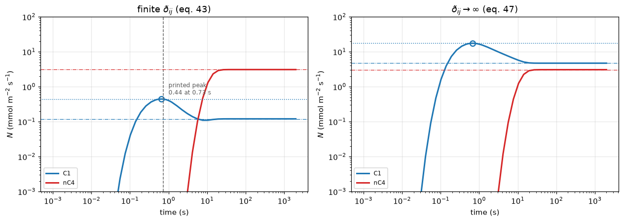
Dash-dot lines are the review's printed steady-state fluxes; the dotted line
is its printed peak. Left and right differ ONLY in whether the two sorbates
feel each other.
4. Against measurement
Bakker measured the nC₄/C₁ permeation selectivity of MFI at both feed compositions. The review quotes both, calls the 95–5 comparison “quite close”, and says nothing about the 50–50 one. Sweeping the upstream composition at constant total pressure puts all of it on one axis.
ys = np.array([0.99, 0.95, 0.80, 0.50, 0.20, 0.05])


def composition_sweep(mode, n_z=30, **kw):
    """S_P over upstream compositions at 100 kPa, each solve warm-started from the last."""
    Th_prev, row = None, []
    for yy in ys:
        m = membrane(n_z=n_z, Dij=mode, **kw)
        p0 = np.array([yy * 1e5, (1 - yy) * 1e5])
        Th_prev, J = m.steady(p0, Th_start=Th_prev)
        row.append(selectivity(J, p0))
    return np.array(row)


SWEEP = {mode: composition_sweep(mode) for mode in ("vignes", "inf")}


def measurement_numbers(sp955, sp5050, sp955i, sp5050i):
    """Model over measurement, and where each measurement sits between the two
    models on a log axis (0 at the infinite-exchange model, 1 at the finite one)."""
    out = {}
    for lab, meas, fin, inf in (("955", MEAS["bakker_95_5"], sp955, sp955i),
                                ("5050", MEAS["bakker_50_50"], sp5050, sp5050i)):
        out[f"bakker_{lab}_model_over_measured"] = fin / meas
        out[f"bakker_{lab}_infinite_over_measured"] = inf / meas
        out[f"bakker_{lab}_infinite_too_low"] = meas / inf
        if fin != inf:      # undefined when the two models coincide (a break row)
            out[f"bakker_{lab}_log_position"] = float(np.log(meas / inf) / np.log(fin / inf))
    return out


MN = measurement_numbers(SP_955, SP_5050, SP_955_INF, SP_5050_INF)
print("Selectivity against MEASUREMENT. This is the only comparison on the page")
print("that is validation rather than reproduction.\n")
print(f"{'feed':>7}{'measured':>10}{'finite Dij':>12}{'ratio':>8}{'infinite Dij':>14}{'ratio':>8}"
      f"{'log position':>14}")
for lab, key, meas, fin, inf in (("95-5", "955", MEAS["bakker_95_5"], SP_955, SP_955_INF),
                                 ("50-50", "5050", MEAS["bakker_50_50"], SP_5050, SP_5050_INF)):
    print(f"{lab:>7}{meas:10.0f}{fin:12.1f}{fin/meas:8.2f}{inf:14.2f}{inf/meas:8.3f}"
          f"{MN[f'bakker_{key}_log_position']:14.2f}")
BAKKER_FIN = [MN["bakker_955_model_over_measured"], MN["bakker_5050_model_over_measured"]]
BAKKER_INF = [MN["bakker_955_infinite_over_measured"], MN["bakker_5050_infinite_over_measured"]]
print(f"\nThe model with finite exchange is {min(BAKKER_FIN):.2f}x to {max(BAKKER_FIN):.2f}x the "
      "measurement;")
print(f"with the exchange removed it is {min(BAKKER_INF):.3f}x to {max(BAKKER_INF):.3f}x, i.e. "
      f"{1/max(BAKKER_INF):.0f}x to {1/min(BAKKER_INF):.0f}x too LOW.")
print("Both measurements lie BETWEEN the two models. 'log position' places each on")
print("a log axis from the infinite-exchange model (0) to the finite one (1): the")
print(f"95-5 point sits at {MN['bakker_955_log_position']:.2f}, close to the finite-exchange "
      f"model, the 50-50 point at {MN['bakker_5050_log_position']:.2f}.")
print("So the data favour finite exchange, clearly at 95-5 and less so at 50-50,")
print("and agree quantitatively with neither model.")
print(f"\nThe review's own words for the 95-5 case are 'quite close', and at "
      f"{BAKKER_FIN[0]:.2f}x that is")
print("defensible. It quotes the 50-50 measurement in the next sentence and does")
print(f"not comment on it; there the finite-exchange model is {BAKKER_FIN[1]:.1f}x high.")
print("Neither number is a fit: nothing in this calculation was tuned to either.")
Selectivity against MEASUREMENT. This is the only comparison on the page
that is validation rather than reproduction.
feed measured finite Dij ratio infinite Dij ratio log position
95-5 380 488.2 1.28 12.36 0.033 0.93
50-50 60 202.9 3.38 5.44 0.091 0.66
The model with finite exchange is 1.28x to 3.38x the measurement;
with the exchange removed it is 0.033x to 0.091x, i.e. 11x to 31x too LOW.
Both measurements lie BETWEEN the two models. 'log position' places each on
a log axis from the infinite-exchange model (0) to the finite one (1): the
95-5 point sits at 0.93, close to the finite-exchange model, the 50-50 point at 0.66.
So the data favour finite exchange, clearly at 95-5 and less so at 50-50,
and agree quantitatively with neither model.
The review's own words for the 95-5 case are 'quite close', and at 1.28x that is
defensible. It quotes the 50-50 measurement in the next sentence and does
not comment on it; there the finite-exchange model is 3.4x high.
Neither number is a fit: nothing in this calculation was tuned to either.fig, ax = plt.subplots(figsize=(6.4, 4.4))
p_nC4 = (1 - ys) * 100.0
ax.semilogy(p_nC4, SWEEP["vignes"], "o-", lw=2.0, color="tab:blue",
label=r"M-S, finite $\eth_{ij}$ (eq. 43)")
ax.semilogy(p_nC4, SWEEP["inf"], "s-", lw=2.0, color="tab:orange",
label=r"M-S, $\eth_{ij}\to\infty$ (eq. 47)")
ax.semilogy([5.0, 50.0], [MEAS["bakker_95_5"], MEAS["bakker_50_50"]], "k*",
ms=15, label="Bakker, measured")
ax.axhline(SP_PURE, color="tab:green", lw=1.3, ls="--",
label=f"pure-component expectation, {SP_PURE}")
ax.set(xlabel="upstream nC4 partial pressure (kPa), total 100 kPa",
ylabel=r"permeation selectivity $S_P$ (eq. 60)",
title="nC4/C1 across MFI at 300 K")
ax.legend(fontsize=8); fig.tight_layout(); plt.show()
print("Every curve here is a prediction from pure-component data alone. The two")
print("stars are the only measured points the review states as numbers.")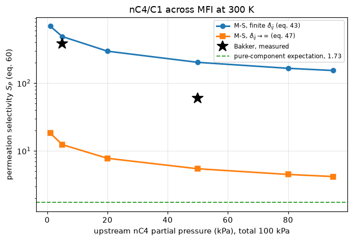
Every curve here is a prediction from pure-component data alone. The two
stars are the only measured points the review states as numbers.
5. The hexane isomers, and the review’s best experimental case
Section 4.3 is the separation the entropy effect was found for. The review takes \(\eth_{n\mathrm{C6}}=5\,\eth_{3\mathrm{MP}}\) after Cavalcante & Ruthven, prints \(S_P = 43.2\) at 33 kPa upstream partial pressures, and reports Funke et al.’s measured value at 15 kPa upstream, against the selectivity for the same pair measured as pure components.
D_RATIO = mprm("nC6", "Section 4.3", "D_ratio_to_3MP")
P_I0 = mprm("mixture", "Section 4.3", "p_i0")


def hex_membrane(ratio=None, n_z=30, isos=None, **kw):
    isos = isos or [NC6, MP3]
    return Membrane(isos, [i.Th_sat for i in isos], [D_RATIO if ratio is None else ratio, 1.0],
                    n_z=n_z, **kw)


def sp_hex(P_total, y_nC6=0.5, ratio=None, n_z=30, isos=None, Th_start=None):
    """S_P of eq. (60) for the nC6/3MP pair, and the bare flux ratio. At an
    equimolar feed the two coincide."""
    m = hex_membrane(ratio, n_z, isos)
    p0 = np.array([y_nC6 * P_total, (1 - y_nC6) * P_total])
    Th_, J = m.steady(p0, Th_start=Th_start)
    Jm = J.mean(0)
    return float(Jm[0] / Jm[1]) / (p0[0] / p0[1]), float(Jm[0] / Jm[1]), Th_


def sp10_crossing(ratio=None, isos=None):
    """Total upstream pressure at which S_P = 10: a direct root on [1, 10] kPa,
    where S_P increases with pressure (the sweep below), ends checked."""
    f = lambda lp: sp_hex(10 ** lp, ratio=ratio, isos=isos)[0] - 10.0
    lo, hi = 3.0, 4.0
    if not f(lo) < 0 < f(hi):
        raise ValueError("S_P = 10 is not bracketed by 1 and 10 kPa")
    return 10 ** brentq(f, lo, hi, xtol=1e-8)


Ps = np.array([1e3, 2e3, 5e3, 15e3, 30e3, 2 * P_I0, 100e3])
Th_prev, SP_hex = None, []
for P in Ps:
    s60, _, Th_prev = sp_hex(P, Th_start=Th_prev)
    SP_hex.append(s60)
SP_hex = np.array(SP_hex)

# the headline point, recomputed from a direct start on each grid and refined
grid = []
for nz in (15, 30, 60):
    m = hex_membrane(n_z=nz)
    _, J = m.steady(np.array([P_I0, P_I0]))
    grid.append((nz, float(J.mean(0)[0] / J.mean(0)[1]), m.flux_spread))
SP_66 = grid[-1][1]
print("nC6/3MP selectivity at the review's condition, grid-refined:")
for nz, v, spread in grid:
    print(f"   n_z = {nz:4d}   S_P = {v:.5f}   flux spread (here {spread:.0e})")
print(f"   the review prints {PRINTED['hex_SP_nC6_3MP']}   "
      f"({(SP_66/PRINTED['hex_SP_nC6_3MP']-1)*100:+.3f} %)")
HEX_SWEEP_VS_DIRECT = abs(SP_hex[list(Ps).index(2 * P_I0)] / grid[1][1] - 1)
print(f"   the same point off the warm-started pressure sweep (n_z = 30): "
      f"(here {HEX_SWEEP_VS_DIRECT:.0e}) from the direct solve")

P_SP10 = sp10_crossing()
print(f"\nS_P crosses 10 at a total upstream pressure of {P_SP10/1e3:.3f} kPa (a root of")
print(f"S_P(P) - 10 on [1, 10] kPa); the review states 'in excess of "
      f"{PRINTED['hex_P_SP10']/1e3:.0f} kPa' ({P_SP10/PRINTED['hex_P_SP10']:.2f}x),")
print("which it reads off its own Fig. 29(c). Scored as a figure-read statement.")

k15 = int(np.where(Ps == 15e3)[0][0])
SP_15 = float(SP_hex[k15])
FUNKE = MEAS["funke_mixture"]
FUNKE_PURE = MEAS["funke_pure"]
print(f"\nAGAINST MEASUREMENT. At the {Ps[k15]/1e3:.0f} kPa upstream pressure of "
      f"Funke et al.'s run:")
print(f"   computed S_P (M-S with finite exchange, IAST) : {SP_15:.2f}")
print(f"   measured by Funke et al.                     : {FUNKE:.1f}   ({(SP_15/FUNKE-1)*100:+.1f} %)")
print(f"   measured by Funke et al. on PURE components  : {FUNKE_PURE}")
print(f"\nThe mixture is {FUNKE/FUNKE_PURE:.0f}x more selective than the pure components in the")
print(f"measurement and {SP_15/FUNKE_PURE:.0f}x in the model, and the model was given nothing but")
print("pure-component isotherm fits and one diffusivity ratio. This is the best")
print("experimental agreement in the review's mixture sections and, unlike")
print("Bakker's methane-butane pair, it is quantitative.")
nC6/3MP selectivity at the review's condition, grid-refined:
n_z = 15 S_P = 43.19499 flux spread (here 1e-13)
n_z = 30 S_P = 43.19983 flux spread (here 3e-13)
n_z = 60 S_P = 43.20092 flux spread (here 4e-13)
the review prints 43.2 (+0.002 %)
the same point off the warm-started pressure sweep (n_z = 30): (here 5e-15) from the direct solve
S_P crosses 10 at a total upstream pressure of 2.505 kPa (a root of
S_P(P) - 10 on [1, 10] kPa); the review states 'in excess of 2 kPa' (1.25x),
which it reads off its own Fig. 29(c). Scored as a figure-read statement.
AGAINST MEASUREMENT. At the 15 kPa upstream pressure of Funke et al.'s run:
computed S_P (M-S with finite exchange, IAST) : 25.03
measured by Funke et al. : 24.0 (+4.3 %)
measured by Funke et al. on PURE components : 1.3
The mixture is 18x more selective than the pure components in the
measurement and 19x in the model, and the model was given nothing but
pure-component isotherm fits and one diffusivity ratio. This is the best
experimental agreement in the review's mixture sections and, unlike
Bakker's methane-butane pair, it is quantitative.Nothing was fitted, but three things were chosen, and the agreement means nothing unless a reader can see them. The review states the measurement in one sentence, “for operation with an upstream pressure of 15 kPa, Funke et al. have experimentally determined a value \(S_P\) of 24”, and states neither the feed composition nor whether 15 kPa is the total or the per-component pressure. Each of the three readings below is worth tens of per cent, which is an order of magnitude more than the agreement being claimed. They are measured rather than argued.
CHOICES = [
    ("AS BUILT: 15 kPa total, equimolar, x5", 15e3, 0.5, 5.0),
    ("  15 kPa EACH instead (30 kPa total)", 30e3, 0.5, 5.0),
    ("  feed y_nC6 = 0.4 instead of 0.5", 15e3, 0.4, 5.0),
    ("  feed y_nC6 = 0.6 instead of 0.5", 15e3, 0.6, 5.0),
    ("  D_nC6 = 4 D_3MP instead of 5", 15e3, 0.5, 4.0),
    ("  D_nC6 = 6 D_3MP instead of 5", 15e3, 0.5, 6.0),
]
print(f"THE THREE CHOICES BEHIND THAT {(SP_15/FUNKE-1)*100:+.1f} %, EACH MEASURED\n")
print(f"{'reading':>40}{'S_P (eq. 60)':>14}{'vs 24':>9}{'flux ratio':>13}")
SENS = []
for lab, Ptot, yy, rr in CHOICES:
    s60, sraw, _ = sp_hex(Ptot, y_nC6=yy, ratio=rr)
    SENS.append((lab, s60, sraw))
    print(f"{lab:>40}{s60:14.2f}{(s60/FUNKE-1)*100:8.0f}%{sraw:13.2f}")


def choice_spread(values):
    return max(values) / min(values)


FUNKE_CHOICE_SPREAD = choice_spread([s for _, s, _ in SENS])
FUNKE_DIRECT_VS_SWEEP = abs(SENS[0][1] / SP_15 - 1)
print(f"\n   The first row is a direct solve and reproduces the {SP_15:.2f} reported above,")
print(f"   which came off a warm-started pressure sweep: (here {FUNKE_DIRECT_VS_SWEEP:.0e}) apart.")
print("   The last column is the bare flux ratio; it differs from S_P only for the")
print("   two non-equimolar rows, where eq. (60) divides out the feed ratio. The")
print(f"   measured {FUNKE:g} is an S_P, so the S_P column is the comparable one, but a")
print("   reader who thinks Funke reported a flux ratio should use the last.")
print(f"\n   spread across the alternatives: {FUNKE_CHOICE_SPREAD:.2f}x, against the "
      f"{abs(SP_15/FUNKE-1)*100:.1f} % agreement claimed.")
print("\nWHY THE READINGS USED ARE THE BETTER-SUPPORTED ONES, and they are still")
print("readings. The review gives the 43.2 point as 'keeping the upstream")
print("compartments at a TOTAL pressure of 66 kPa' while the Fig. 29(a) caption")
print("gives the same condition as p_i0 = 33 kPa, so in this paper an upstream")
print("pressure quoted in running text is a total; and the S_P > 10 threshold is")
print("stated as 'the pressure in the upstream compartment increases beyond 2 kPa'")
print(f"against the {P_SP10/1e3:.2f} kPa TOTAL computed above. Equimolar is the "
      "composition of every")
print("simulation in Section 4.3 and the curve the review places Funke's square")
print("on. Neither is stated for the MEASUREMENT, and the review does not say")
print(f"what Funke's feed was. The last two rows are not readings at all (the")
print(f"ratio of {D_RATIO:g} IS printed), but it is a single experimental number from a")
print("third paper (Cavalcante & Ruthven, recorded under origin_not_consulted and")
print("not opened here), and it drives the whole hexane result.")
print(f"\nSo: nothing was tuned, and the {(SP_15/FUNKE-1)*100:+.1f} % should be read as one "
      "point inside")
print(f"a {FUNKE_CHOICE_SPREAD:.1f}x band of defensible readings, against a measurement printed "
      "to two")
print("significant figures with no stated uncertainty.")
THE THREE CHOICES BEHIND THAT +4.3 %, EACH MEASURED
reading S_P (eq. 60) vs 24 flux ratio
AS BUILT: 15 kPa total, equimolar, x5 25.03 4% 25.03
15 kPa EACH instead (30 kPa total) 33.11 38% 33.11
feed y_nC6 = 0.4 instead of 0.5 22.56 -6% 15.04
feed y_nC6 = 0.6 instead of 0.5 27.18 13% 40.77
D_nC6 = 4 D_3MP instead of 5 21.07 -12% 21.07
D_nC6 = 6 D_3MP instead of 5 28.94 21% 28.94
The first row is a direct solve and reproduces the 25.03 reported above,
which came off a warm-started pressure sweep: (here 7e-16) apart.
The last column is the bare flux ratio; it differs from S_P only for the
two non-equimolar rows, where eq. (60) divides out the feed ratio. The
measured 24 is an S_P, so the S_P column is the comparable one, but a
reader who thinks Funke reported a flux ratio should use the last.
spread across the alternatives: 1.57x, against the 4.3 % agreement claimed.
WHY THE READINGS USED ARE THE BETTER-SUPPORTED ONES, and they are still
readings. The review gives the 43.2 point as 'keeping the upstream
compartments at a TOTAL pressure of 66 kPa' while the Fig. 29(a) caption
gives the same condition as p_i0 = 33 kPa, so in this paper an upstream
pressure quoted in running text is a total; and the S_P > 10 threshold is
stated as 'the pressure in the upstream compartment increases beyond 2 kPa'
against the 2.51 kPa TOTAL computed above. Equimolar is the composition of every
simulation in Section 4.3 and the curve the review places Funke's square
on. Neither is stated for the MEASUREMENT, and the review does not say
what Funke's feed was. The last two rows are not readings at all (the
ratio of 5 IS printed), but it is a single experimental number from a
third paper (Cavalcante & Ruthven, recorded under origin_not_consulted and
not opened here), and it drives the whole hexane result.
So: nothing was tuned, and the +4.3 % should be read as one point inside
a 1.6x band of defensible readings, against a measurement printed to two
significant figures with no stated uncertainty.D32 = mprm("3MP", "Section 4.3", "D_ratio_to_22DMB")
D_TERN = mprm("ternary", "Section 4.3", "D_ratio_nC6_to_22DMB")
def dmb_numbers(d32=D32, d_tern=D_TERN):
"""3MP/2,2DMB permeation selectivity, binary at 30 kPa each, and with nC6
present (ternary, reached by warm starts from 2 and 10 kPa total)."""
m = Membrane([MP3, DMB], [MP3.Th_sat, DMB.Th_sat], [d32, 1.0], n_z=30)
_, J = m.steady(np.array([30e3, 30e3]))
sp_bin = float(J.mean(0)[0] / J.mean(0)[1])
Th_p = None
for P in (2e3, 1e4, 9e4):
m3 = Membrane([NC6, MP3, DMB], [NC6.Th_sat, MP3.Th_sat, DMB.Th_sat],
[d_tern, d_tern, 1.0], n_z=30)
Th_p, J3 = m3.steady(np.full(3, P / 3), Th_start=Th_p)
sp_tern = float(J3.mean(0)[1] / J3.mean(0)[2])
return sp_bin, sp_tern
SP_BIN, SP_TERN = dmb_numbers()
print("The other two hexane cases the review quotes, both read off ITS OWN")
print("figures rather than printed as computed results:\n")
print(f" 3MP/2,2DMB, binary, 30 kPa each : computed {SP_BIN:6.2f} "
f"the review says {PRINTED['hex_SP_3MP_DMB_binary']:.0f}"
f" ({(SP_BIN/PRINTED['hex_SP_3MP_DMB_binary']-1)*100:+.0f} %)")
print(f" the same pair with nC6 present : computed {SP_TERN:6.2f} "
f"the review says 'in excess of {PRINTED['hex_SP_3MP_DMB_ternary']:.0f}'"
f" (satisfied: {SP_TERN > PRINTED['hex_SP_3MP_DMB_ternary']})")
print(f"\nAdding nC6 raises the 3MP/2,2DMB selectivity by {SP_TERN/SP_BIN:.1f}x here, against the")
print(f"review's own factor of at least "
f"{PRINTED['hex_SP_3MP_DMB_ternary']/PRINTED['hex_SP_3MP_DMB_binary']:.1f}x. "
"The mechanism is reproduced; the two numbers")
print("are figure readings by the authors on a log axis and are not scored with")
print("the printed results.")The other two hexane cases the review quotes, both read off ITS OWN
figures rather than printed as computed results:
3MP/2,2DMB, binary, 30 kPa each : computed 8.43 the review says 7 (+20 %)
the same pair with nC6 present : computed 82.37 the review says 'in excess of 30' (satisfied: True)
Adding nC6 raises the 3MP/2,2DMB selectivity by 9.8x here, against the
review's own factor of at least 4.3x. The mechanism is reproduced; the two numbers
are figure readings by the authors on a log axis and are not scored with
the printed results.fig, axes = plt.subplots(1, 2, figsize=(11.6, 4.2))
axes[0].loglog(Ph / 1e3, Thh[:, 0], lw=2.0, color="tab:blue", label=r"nC6")
axes[0].loglog(Ph / 1e3, Thh[:, 1], lw=2.0, color="tab:red", label=r"3MP")
axes[0].loglog(Ph / 1e3, Thh.sum(1), lw=1.3, ls="--", color="0.4", label=r"$\Theta_{\rm mix}$")
axes[0].axhline(4.0, color="0.4", lw=1.0, ls=":")
axes[0].axvline(P_TH4 / 1e3, color="tab:green", lw=1.0)
axes[0].annotate(f"$\\Theta_{{\\rm mix}}=4$ at {P_TH4/1e3:.2f} kPa",
(P_TH4 / 1e3 * 1.3, 0.02), fontsize=8, color="tab:green")
axes[0].set(xlabel="total upstream pressure (kPa)",
ylabel=r"$\Theta$ (molecules per unit cell)", ylim=(1e-2, 20),
title="50-50 nC6/3MP sorption at 362 K (IAST)")
axes[0].legend(fontsize=8, loc="upper left")
axes[1].loglog(Ps / 1e3, SP_hex, "o-", lw=2.0, color="tab:blue", label="M-S + IAST, this page")
axes[1].plot([15.0], [FUNKE], "k*", ms=15, label="Funke et al., mixture")
axes[1].plot([15.0], [FUNKE_PURE], "ko", ms=9, mfc="none", mew=1.8,
label="Funke et al., pure components")
axes[1].plot([2 * P_I0 / 1e3], [PRINTED["hex_SP_nC6_3MP"]], "P", ms=11,
color="tab:red", label=f"the review's printed {PRINTED['hex_SP_nC6_3MP']}")
axes[1].axhline(10.0, color="0.5", lw=1.0, ls=":")
axes[1].set(xlabel="total upstream pressure (kPa)", ylabel=r"$S_P$ (nC6 over 3MP)",
title="nC6/3MP permeation selectivity at 362 K")
axes[1].legend(fontsize=8, loc="upper left")
fig.tight_layout(); plt.show()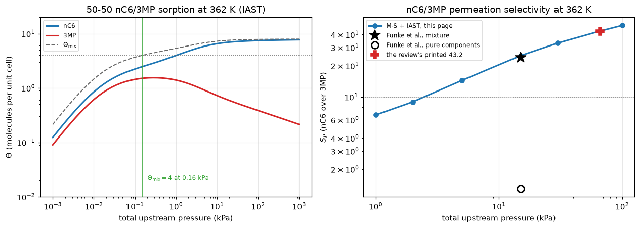
6. Two counterfactuals the review states, and what they actually give
The multicomponent Langmuir. The review says that with eq. (39) and the saturation capacities of C1 and nC4 set equal, \(S_P\) “would be predicted to be independent of the upstream composition and have a constant value of 800”. That is two claims again, a structural one and a numerical one, and they come apart.
The zeolite 4A counter-example. Section 4.4 is the case that goes the other way, and a page showing only finite \(\eth_{ij}\) winning would misreport the review’s own conclusion.
LANG_YS = (0.95, 0.80, 0.50, 0.20, 0.05)


def langmuir_sweep(cap_c1=10.0, cap_nc4=10.0, scale_bA_nc4=1.0, ys_=LANG_YS):
    """S_P with the multicomponent Langmuir (eq. 39), single-site with the Table 1
    site-A affinities and the given capacities."""
    out = []
    for yy in ys_:
        m = Membrane([DSL(C1.bA, cap_c1), DSL(NC4.bA * scale_bA_nc4, cap_nc4)],
                     [cap_c1, cap_nc4], [D_C1, D_NC4], n_z=30, iso_model="langmuir")
        p0 = np.array([yy * 1e5, (1 - yy) * 1e5])
        out.append(selectivity(m.steady(p0)[1], p0))
    return np.array(out)


LANG = langmuir_sweep()             # "the saturation capacities set equal to one another"
LANG_SPREAD = float(LANG.max() / LANG.min())
LANG_MEAN = float(np.mean(LANG))
print("Multicomponent Langmuir, eq. (39), equal saturation capacities:")
print(f"{'upstream y_C1':>15}{'S_P':>12}")
for yy, v in zip(LANG_YS, LANG):
    print(f"{yy:15.2f}{v:12.2f}")
IAST_SPREAD = float(SWEEP["vignes"][1:].max() / SWEEP["vignes"][1:].min())
print(f"\n   spread from 95 % down to 5 % methane in the feed: {LANG_SPREAD:.3f}x")
print(f"   IAST over exactly the same five feeds:            {IAST_SPREAD:.1f}x")
print("   -> THE STRUCTURAL CLAIM IS REPRODUCED. The multicomponent Langmuir")
print(f"      keeps S_P within {(LANG_SPREAD-1)*100:.1f} % across the five feeds, and IAST "
      "does not.")
print("      That is exactly the review's argument for IAST.")
print(f"\n   the VALUE, however, is {LANG_MEAN:.0f} here against the printed "
      f"{PRINTED['mix_SP_langmuir']:.0f} ({LANG_MEAN/PRINTED['mix_SP_langmuir']:.2f}x).")
print("   The review does not say which saturation capacity it set the two equal")
print("   TO, nor which affinity it used once the dual-site fit is collapsed to a")
print("   single site. The first turns out not to matter (with equal capacities")
print("   the occupancies are independent of their common value and Theta_sat")
print("   cancels out of the flux ratio, checked below) but the second does. The")
print("   Table 1 site-A affinities are used here and the counterfactual is")
print("   reported as UNREPRODUCED rather than tuned until it lands on 800.")


def langmuir_capacity_check(cap_a, cap_b):
    """S_P at 50-50 with capacities cap_a and cap_b against both at 19."""
    a = langmuir_sweep(cap_a, cap_b, ys_=(0.5,))[0]
    b = langmuir_sweep(19.0, 19.0, ys_=(0.5,))[0]
    return a, b, abs(a / b - 1)


LC_A, LC_B, LANG_CAP_DEV = langmuir_capacity_check(4.0, 4.0)
print(f"\n   (Theta_sat = 4 vs 19 at 50-50: {LC_A:.3f} vs {LC_B:.3f}, (here {LANG_CAP_DEV:.0e}) apart)")
Multicomponent Langmuir, eq. (39), equal saturation capacities:
upstream y_C1 S_P
0.95 1652.29
0.80 1684.10
0.50 1690.55
0.20 1692.17
0.05 1692.59
spread from 95 % down to 5 % methane in the feed: 1.024x
IAST over exactly the same five feeds: 3.2x
-> THE STRUCTURAL CLAIM IS REPRODUCED. The multicomponent Langmuir
keeps S_P within 2.4 % across the five feeds, and IAST does not.
That is exactly the review's argument for IAST.
the VALUE, however, is 1682 here against the printed 800 (2.10x).
The review does not say which saturation capacity it set the two equal
TO, nor which affinity it used once the dual-site fit is collapsed to a
single site. The first turns out not to matter (with equal capacities
the occupancies are independent of their common value and Theta_sat
cancels out of the flux ratio, checked below) but the second does. The
Table 1 site-A affinities are used here and the counterfactual is
reported as UNREPRODUCED rather than tuned until it lands on 800.
(Theta_sat = 4 vs 19 at 50-50: 1690.551 vs 1690.551, (here 0e+00) apart)The review’s conclusion 9 goes the other way for zeolite 4A, and it is quoted here rather than paraphrased into agreement. Section 4.4 compares both implementations against Habgood’s measured N₂/CH₄ uptake in 4A and finds that “the M–S model, assuming \(\eth_{ij}\to\infty\), does a very good job”, concluding that diffusion of N₂ and CH₄ in 4A “is essentially free from vacancy correlation effects”. The physical reason the review gives is topological: in 4A the intracage hopping is fast and is not the limiting step, whereas in MFI the exchange happens at the channel intersections and is not fast.
So the finding is not “finite \(\eth_{ij}\) is right”. It is that \(\eth_{ij}\) is a property of the host topology, and MFI and 4A land at opposite limits of it. That case cannot be reproduced here: its only validation is Figs. 32–34, and the review prints no numerical result for it. It is scoped out for exactly the reason the rest of Sections 4.4–4.7 are.
7. Self-diffusivity, where the correlation effect is largest
Eqs. (53)–(56). The self-diffusivity contains no \([\Gamma]\) at all, so it isolates the exchange coefficients from the sorption thermodynamics, which is why the review uses it to argue that correlation effects are real. There is no printed number to check against; the comparison is Fig. 21.
TS = np.array([mprm("CH4", "Section 3.4", "Theta_sat"), mprm("CF4", "Section 3.4", "Theta_sat")])
D0S = np.array([mprm("CH4", "Section 3.4", "D_MS_0"), mprm("CF4", "Section 3.4", "D_MS_0")])
TTOT = mprm("mixture", "Section 3.4", "Theta_total")
LOADS_CH4 = (1.0, 3.0, 6.0, 9.0, 11.0)


def D_self(Th, D0, Th_sat, facile=False):
    """eq. (56). D_11 = D_1 by eq. (43) applied at i = j, an algebraic
    identity used here only because the review does."""
    th = Th / Th_sat
    D_i = D0 * (1 - th.sum())                     # eq. (19) on the total occupancy
    out = []
    for i in (0, 1):
        j = 1 - i
        if facile:
            out.append(D_i[i])
            continue
        xi = th[i] / (th[i] + th[j])
        Dij = D_i[i] ** xi * D_i[j] ** (1 - xi)
        out.append(1.0 / (1 / D_i[i] + th[i] / D_i[i] + th[j] / Dij))
    return np.array(out)


def self_ratios(ts=TS):
    r = []
    for T1 in LOADS_CH4:
        T = np.array([T1, TTOT - T1])
        r.append(D_self(T, D0S, ts, facile=True)[0] / D_self(T, D0S, ts)[0])
    return float(min(r)), float(max(r))


print(f"Snurr & Karger's CH4/CF4 in MFI at 200 K, total loading {TTOT:.0f} "
      "molecules per unit cell")
print(f"(Theta_sat = {TS[0]:.0f} and {TS[1]:.0f}; D(0) = {D0S[0]:.1e} and {D0S[1]:.1e} m2/s)\n")
print(f"{'Theta_CH4':>10}{'D*_CH4':>12}{'facile':>12}{'ratio':>8}"
      f"{'D*_CF4':>12}{'facile':>12}{'ratio':>8}")
for T1 in LOADS_CH4:
    T = np.array([T1, TTOT - T1])
    a = D_self(T, D0S, TS); b = D_self(T, D0S, TS, facile=True)
    print(f"{T1:10.1f}{a[0]:12.3e}{b[0]:12.3e}{b[0]/a[0]:8.2f}"
          f"{a[1]:12.3e}{b[1]:12.3e}{b[1]/a[1]:8.2f}")
SELF_RATIO = self_ratios()
print(f"\nRemoving the exchange raises the methane self-diffusivity by "
      f"{SELF_RATIO[0]:.1f}x to {SELF_RATIO[1]:.1f}x.")
print("The review states that the dotted facile-exchange lines of its Fig. 21(b)")
print("lie well above the MD points while the finite-exchange lines of Fig. 21(a)")
print("agree, but it prints no number for either, so THIS COMPARISON HAS NO")
print("TARGET. What is shown is the size and sign of the effect the review")
print("attributes to correlation, not evidence that the review is right about it.")
print("\nONE CHOICE IS MADE SILENTLY BY EQ. (19) AND IS STATED HERE INSTEAD.")
print("Eq. (19) as printed is D_i = D_i(0)(1 - Theta_i/Theta_i,sat), the species'")
print("OWN occupancy. The cell above uses D0 * (1 - sum_k theta_k), the TOTAL")
print("occupancy, which is a generalisation to a mixture that the review states")
print("nowhere; Section 3.4 says only 'Eqs. (19), (43) and (56)'. The RATIOS")
print("above do not depend on it: a factor common to both species' D_i scales")
print("D_ij by the same factor (eq. 43), so it cancels from facile/finite. The")
print("self-diffusivities themselves do depend on it, by the factor:")
for T1 in (1.0, 6.0, 11.0):
    T = np.array([T1, TTOT - T1]); th = T / TS
    print(f"      Theta_CH4 = {T1:4.1f}:  1 - theta_total = {1-th.sum():.4f}   "
          f"1 - theta_CH4 = {1-th[0]:.4f}   ({(1-th[0])/(1-th.sum()):.2f}x)")
print("\nTwo relations used above are ALGEBRAIC IDENTITIES and are not checks:")
print("  eq. (43) at i = j returns D_ii = D_i, which is what x^a y^(1-a) does")
print("  when y = x; and eq. (55), D*_1 = D_1/(1+theta_1), is eq. (54) with")
print("  D_11 = D_1 substituted and the other terms dropped. Both are stated")
print("  because the review uses them; neither is scored.")
Snurr & Karger's CH4/CF4 in MFI at 200 K, total loading 12 molecules per unit cell
(Theta_sat = 22 and 13; D(0) = 6.0e-09 and 2.5e-09 m2/s)
Theta_CH4 D*_CH4 facile ratio D*_CF4 facile ratio
1.0 2.177e-10 6.503e-10 2.99 1.434e-10 2.710e-10 1.89
3.0 3.992e-10 1.028e-09 2.57 2.366e-10 4.283e-10 1.81
6.0 7.692e-10 1.594e-09 2.07 4.006e-10 6.643e-10 1.66
9.0 1.252e-09 2.161e-09 1.73 6.148e-10 9.003e-10 1.46
11.0 1.600e-09 2.538e-09 1.59 8.068e-10 1.058e-09 1.31
Removing the exchange raises the methane self-diffusivity by 1.6x to 3.0x.
The review states that the dotted facile-exchange lines of its Fig. 21(b)
lie well above the MD points while the finite-exchange lines of Fig. 21(a)
agree, but it prints no number for either, so THIS COMPARISON HAS NO
TARGET. What is shown is the size and sign of the effect the review
attributes to correlation, not evidence that the review is right about it.
ONE CHOICE IS MADE SILENTLY BY EQ. (19) AND IS STATED HERE INSTEAD.
Eq. (19) as printed is D_i = D_i(0)(1 - Theta_i/Theta_i,sat), the species'
OWN occupancy. The cell above uses D0 * (1 - sum_k theta_k), the TOTAL
occupancy, which is a generalisation to a mixture that the review states
nowhere; Section 3.4 says only 'Eqs. (19), (43) and (56)'. The RATIOS
above do not depend on it: a factor common to both species' D_i scales
D_ij by the same factor (eq. 43), so it cancels from facile/finite. The
self-diffusivities themselves do depend on it, by the factor:
Theta_CH4 = 1.0: 1 - theta_total = 0.1084 1 - theta_CH4 = 0.9545 (8.81x)
Theta_CH4 = 6.0: 1 - theta_total = 0.2657 1 - theta_CH4 = 0.7273 (2.74x)
Theta_CH4 = 11.0: 1 - theta_total = 0.4231 1 - theta_CH4 = 0.5000 (1.18x)
Two relations used above are ALGEBRAIC IDENTITIES and are not checks:
eq. (43) at i = j returns D_ii = D_i, which is what x^a y^(1-a) does
when y = x; and eq. (55), D*_1 = D_1/(1+theta_1), is eq. (54) with
D_11 = D_1 substituted and the other terms dropped. Both are stated
because the review uses them; neither is scored.Validation
This page has both kinds of comparison and keeps them apart in the words used. Four numbers are measurements (Bakker’s two and Funke’s two) and comparing against them is validation. Everything else is a number Krishna & Baur computed, and comparing against those is reproduction.
Five groups of checks with something to fail against, then the break table, which re-runs each computation with a defect injected and records which claims catch it.
print("1. The IAST solve, three ways it can be wrong\n")
P_RT = np.array([[95e3, 5e3], [1e3, 1e3], [1e-2, 1e-4], [5e5, 5e5]])


def roundtrip(forward_iast, inverse_iast):
    Th_rt = forward_iast.forward(P_RT)
    return float(np.max(np.abs(inverse_iast.inverse(Th_rt) / P_RT - 1)))


IAST_ROUNDTRIP = roundtrip(mix, mix)
print(f"   (a) forward (p)->(Theta) then inverse (Theta)->(p), 4 states: (here {IAST_ROUNDTRIP:.0e})")
print("       tests the inverse against the forward. It CANNOT see an error")
print("       common to both (the surface potential, which is (b)).")


def psi_vs_quadrature(isos, drop_site_B=False):
    worst = 0.0
    for it in isos:
        for P in (1e-2, 1e2, 1e5, 1e7):
            num = quad(lambda x: it.theta(x) / x, 1e-14, P, limit=400)[0]
            closed = it.tA * np.log1p(it.bA * P) if drop_site_B else it.psi(P)
            worst = max(worst, abs(closed / num - 1))
    return float(worst)


PSI_QUAD = psi_vs_quadrature((C1, NC4, NC6, MP3))
print(f"\n   (b) eq. (64) in closed form against adaptive quadrature of Theta^0(P)/P,\n"
      f"       4 isotherms x 4 pressures: (here {PSI_QUAD:.0e})")
print("       This one CAN fail: the quadrature never sees the log form.")


def iast_vs_langmuir(cap_a, cap_b):
    """IAST against the multicomponent Langmuir for two single-site isotherms."""
    ea, eb = DSL(NC4.bA, cap_a), DSL(C1.bA, cap_b)
    lm = IAST([ea, eb])
    worst = 0.0
    for Ptot in np.logspace(-2, 7, 19):
        for yy in (0.05, 0.5, 0.95):
            p = np.array([[yy * Ptot, (1 - yy) * Ptot]])
            T = lm.forward(p)[0]
            den = 1 + ea.bA * p[0, 0] + eb.bA * p[0, 1]
            L = np.array([cap_a * ea.bA * p[0, 0] / den, cap_b * eb.bA * p[0, 1] / den])
            worst = max(worst, float(np.max(np.abs(T / L - 1))))
    return worst


IAST_LANGMUIR = iast_vs_langmuir(6.0, 6.0)
IAST_UNEQUAL = iast_vs_langmuir(NC4.Th_sat, C1.Th_sat)
print(f"\n   (c) IAST vs the multicomponent Langmuir with EQUAL saturation")
print(f"       capacities, 19 pressures x 3 compositions : (here {IAST_LANGMUIR:.0e})")
print(f"       the same comparison with the Table 1 capacities ({NC4.Th_sat:.0f} and "
      f"{C1.Th_sat:.0f}): {IAST_UNEQUAL*100:.0f} %")
print("       The first is the theorem the review relies on and it is a real test")
print("       of the IAST solve: a wrong surface potential breaks it. The second")
print("       says the theorem does not apply to this system, which is the whole")
print("       reason IAST is needed.")
1. The IAST solve, three ways it can be wrong
(a) forward (p)->(Theta) then inverse (Theta)->(p), 4 states: (here 3e-14)
tests the inverse against the forward. It CANNOT see an error
common to both (the surface potential, which is (b)).
(b) eq. (64) in closed form against adaptive quadrature of Theta^0(P)/P,
4 isotherms x 4 pressures: (here 1e-12)
This one CAN fail: the quadrature never sees the log form.
(c) IAST vs the multicomponent Langmuir with EQUAL saturation
capacities, 19 pressures x 3 compositions : (here 1e-15)
the same comparison with the Table 1 capacities (10 and 19): 15047 %
The first is the theorem the review relies on and it is a real test
of the IAST solve: a wrong surface potential breaks it. The second
says the theorem does not apply to this system, which is the whole
reason IAST is needed.print("2. [Gamma] and [B], each by two routes that share no code\n")
TS_V = np.array([C1.Th_sat, NC4.Th_sat])
states = mix.forward(np.logspace(1, 6.5, 12)[:, None] * Y)
G_nu = gamma_numerical(mix, states, TS_V)
def gamma_two_routes(drop_mix_term=False):
G_an = mix.inverse_and_gamma(states, TS_V, drop_mix_term=drop_mix_term)[1]
return float(np.max(np.abs(G_an / G_nu - 1)))
GAMMA_TWO_ROUTES = gamma_two_routes()
print(f" [Gamma] by implicit differentiation of eqs. (62)-(65) against central")
print(f" differences of the IAST inverse map, 12 states x 4 elements: (here {GAMMA_TWO_ROUTES:.0e})")
print(" (the finite-difference floor; the break table moves it to O(1))")
print(" WHAT IT CANNOT SEE: both routes call the same IAST solve, so an error")
print(" inside eqs. (62)-(65) moves them together. That is what check 1 is for.")
rng = np.random.default_rng(20260803)
FR_STATES = []
for _ in range(200):
n = int(rng.integers(2, 4))
FR_STATES.append((rng.uniform(0.01, 0.30, n), 10.0 ** rng.uniform(-11, -9, n),
rng.normal(size=n)))
def friction_routes(defect=None):
"""Worst gap between the matrix-free eq. (42) and eq. (44)'s [B] inverted;
``defect`` "diag" drops the exchange sum from B_ii, "offdiag" zeroes B_ij."""
worst = 0.0
for th, D, d in FR_STATES:
B = B_matrix(th[None, :], D[None, :])[0]
if defect == "diag":
B[np.diag_indices_from(B)] = 1.0 / D
elif defect == "offdiag":
B = np.diag(np.diag(B))
worst = max(worst, float(np.max(np.abs(friction_solve(th, D, d) / np.linalg.solve(B, d) - 1))))
return worst
FRICTION_TWO_ROUTES = friction_routes()
FRICTION_BROKEN = friction_routes("diag")
print(f"\n eq. (44)'s [B], assembled and inverted, against the raw friction")
print(f" system of eq. (42) solved matrix-free by GMRES, 200 random 2- and")
print(f" 3-component states: (here {FRICTION_TWO_ROUTES:.0e})")
print(f" with the exchange sum dropped from B_ii: {FRICTION_BROKEN*100:.0f} %")
print(" The GMRES route never forms [B], so it cannot inherit an error in the")
print(" B_ii / B_ij formulas. This is A4.2's replacement for a check that")
print(" compared [B] against itself, reused.")
th1 = np.array([[0.37]])
B1 = B_matrix(th1, np.array([[D_C1]]))[0]
G1 = np.array([[2.4]])
COLLAPSE_46 = float(abs((np.linalg.solve(B1, G1))[0, 0] / (D_C1 * G1[0, 0]) - 1))
print(f"\n eq. (46) at n = 1 against eq. (14), D = eth Gamma: (here {COLLAPSE_46:.0e})")
print(" ALGEBRAIC IDENTITY, labelled as one: at n = 1 the sum in eq. (44) is")
print(" empty so [B] = 1/eth by construction. It confirms the indexing of the")
print(f" code and nothing else. The collapse that CAN fail is the one in")
print(f" Results, where the n = 1 SOLVER is run against the closed-form")
print(f" eq. (12) integral: {COLLAPSE_1:.1e}.")2. [Gamma] and [B], each by two routes that share no code
[Gamma] by implicit differentiation of eqs. (62)-(65) against central
differences of the IAST inverse map, 12 states x 4 elements: (here 2e-07)
(the finite-difference floor; the break table moves it to O(1))
WHAT IT CANNOT SEE: both routes call the same IAST solve, so an error
inside eqs. (62)-(65) moves them together. That is what check 1 is for.
eq. (44)'s [B], assembled and inverted, against the raw friction
system of eq. (42) solved matrix-free by GMRES, 200 random 2- and
3-component states: (here 6e-14)
with the exchange sum dropped from B_ii: 687 %
The GMRES route never forms [B], so it cannot inherit an error in the
B_ii / B_ij formulas. This is A4.2's replacement for a check that
compared [B] against itself, reused.
eq. (46) at n = 1 against eq. (14), D = eth Gamma: (here 2e-16)
ALGEBRAIC IDENTITY, labelled as one: at n = 1 the sum in eq. (44) is
empty so [B] = 1/eth by construction. It confirms the indexing of the
code and nothing else. The collapse that CAN fail is the one in
Results, where the n = 1 SOLVER is run against the closed-form
eq. (12) integral: 1.1e-04.print("3. Discretisation, the solver, and the two modelling choices the review leaves open\n")
GRID = []
for nz in (20, 40, 80, 160):
m = membrane(n_z=nz)
_, J = m.steady(FEEDS["95-5"])
GRID.append((nz, selectivity(J, FEEDS["95-5"]), m.flux_spread))
print(f" {'n_z':>6}{'S_P':>14}{'change from n_z/2':>19}{'flux spread':>14}")
for k, (nz, v, spr) in enumerate(GRID):
ch = f"{v/GRID[k-1][1]-1:19.2e}" if k else f"{'-':>19}"
print(f" {nz:6d}{v:14.6f}{ch} (here {spr:.0e})")
SG = {nz: v for nz, v, _ in GRID}
STEADY_ORDER = grid_order(SG[40], SG[80], SG[160])
STEADY_ORDER_COARSE = grid_order(SG[20], SG[40], SG[80])
STEADY_RICH = richardson(SG[160], SG[80], STEADY_ORDER)
GRID_ERR = abs(SG[40] / STEADY_RICH - 1)
STEADY_DIFF_OVER_TOL = abs(SG[80] - SG[160]) / (1e-9 * SG[160])
print(f" observed order {STEADY_ORDER_COARSE:.2f} (20/40/80) and {STEADY_ORDER:.2f} (40/80/160),")
print(f" from successive differences; Richardson on the last pair puts the")
print(f" steady production runs (n_z = 40) {GRID_ERR*100:.4f} % from the grid limit,")
print(" far below every steady deviation reported above. The flux spread is")
print(" div N at steady state and is checked on every solve.")
print("\n WHAT THIS STUDY DOES NOT COVER: the TRANSIENT. The steady loading")
print(" profile is smooth, so it converges quickly and cheaply here; the")
print(" transient carries a self-sharpening n-butane front and needs a finer")
print(f" grid. That is refined separately, in Results, at n_z = {NZ_PROD}. A grid")
print(" study is only evidence for the solution it was run on.")
STEADY_GRID_NOTE = (f"steady S_P at n_z = 40 is {GRID_ERR:.0e} from its grid limit, "
f"the transient peak time {abs(gv[30][0]/T_RICH-1)*100:.0f} % at n_z = 30")
print(f" ({STEADY_GRID_NOTE})")
print("\n The solver. Every production solve converged directly from the linear")
print(f" profile: {N_CONTINUED} of {len(RUNS)} needed the continuation route. The")
print(" continuation route is run on the 95-5 feed anyway and compared:")
def path_dev(target_factor=1.0):
"""The 95-5 solve by continuation (to ``target_factor`` of the feed pressures,
1 unless the break table injects a short path) against the direct solve."""
m_b = membrane(n_z=NZ_STEADY)
_, J_b = m_b.steady(FEEDS["95-5"] * target_factor, force_continuation=True)
return abs(selectivity(J_b, FEEDS["95-5"]) / SP_955 - 1), m_b
PATH_DEV, m_b = path_dev()
print(f" direct : S_P = {SP_955:.9f}")
print(f" continuation : S_P = {SP_955*(1+PATH_DEV):.9f} (here {PATH_DEV:.0e}), "
f"{len(m_b.result.history)} Newton iterations at the last value)")
print("\n The downstream pressure ('vanishing values by means of a sweep gas'):")
def pd_numbers(fracs):
out = []
for f_ in fracs:
m = membrane(n_z=30, pd_frac=f_)
_, J = m.steady(FEEDS["95-5"])
out.append((f_, selectivity(J, FEEDS["95-5"]), m.flux_spread))
return out
PD = pd_numbers((1e-4, 1e-5, 1e-6, 1e-7, 1e-8, 1e-10))
for f_, v, spr in PD:
print(f" p_delta/p_0 = {f_:.0e} S_P = {v:.4f} flux spread (here {spr:.0e})")
PDD = {f_: v for f_, v, _ in PD}
PD_SENS = abs(PDD[1e-4] / PDD[1e-7] - 1)
PD_SENS_DEEP = abs(PDD[1e-7] / PDD[1e-10] - 1)
PD_DECADES_BELOW = int(round(np.log10(1e-6 / min(PDD))))
print(f" three decades of sweep pressure (1e-4 to 1e-7) move S_P by {PD_SENS*100:.5f} %,")
print(f" and 1e-7 to 1e-10 by {PD_SENS_DEEP:.1e}, linear in the downstream pressure. Every")
print(f" solve converges, down to {PD_DECADES_BELOW} decades below the production value of 1e-6.")
print("\n The loading dependence of eth, which Section 3.2 leaves as 'e.g.")
print(" eq. (17) or eq. (19)' and never fixes for the membrane:")
DEPS = (("eq. (17), constant", None),
("eq. (19), eth(0)(1-theta_i)", lambda th: 1.0 - th),
("eq. (19) on the TOTAL occupancy",
lambda th: np.repeat((1.0 - th.sum(-1))[:, None], th.shape[-1], -1)))
def loading_dep_runs(D0=None):
out = {}
for lab, dep in DEPS:
m = membrane(n_z=30, loading_dep=dep, D0=D0)
out[lab] = selectivity(m.steady(FEEDS["95-5"])[1], FEEDS["95-5"])
return out
ALT = loading_dep_runs()
for lab, v in ALT.items():
print(f" {lab:35s} S_P = {v:8.2f} ({v/PRINTED['mix_SP_955_finite']-1:+.1%} vs printed)")
DEP_SPREAD = max(ALT.values()) / min(ALT.values())
print(f" {DEP_SPREAD:.2f}x between the readings. eq. (17) is the one that")
print(" reproduces the printed selectivity and the one A4.7 established for the")
print(" single components, so it is the production choice; the review does")
print(" not say so, and the other readings are not far off either.")3. Discretisation, the solver, and the two modelling choices the review leaves open
n_z S_P change from n_z/2 flux spread
20 488.153064 - (here 5e-14)
40 488.231467 1.61e-04 (here 1e-13)
80 488.249910 3.78e-05 (here 2e-13)
160 488.254368 9.13e-06 (here 1e-12)
observed order 2.09 (20/40/80) and 2.05 (40/80/160),
from successive differences; Richardson on the last pair puts the
steady production runs (n_z = 40) 0.0050 % from the grid limit,
far below every steady deviation reported above. The flux spread is
div N at steady state and is checked on every solve.
WHAT THIS STUDY DOES NOT COVER: the TRANSIENT. The steady loading
profile is smooth, so it converges quickly and cheaply here; the
transient carries a self-sharpening n-butane front and needs a finer
grid. That is refined separately, in Results, at n_z = 120. A grid
study is only evidence for the solution it was run on.
(steady S_P at n_z = 40 is 5e-05 from its grid limit, the transient peak time 11 % at n_z = 30)
The solver. Every production solve converged directly from the linear
profile: 0 of 4 needed the continuation route. The
continuation route is run on the 95-5 feed anyway and compared:
direct : S_P = 488.231467016
continuation : S_P = 488.231467016 (here 3e-16), 6 Newton iterations at the last value)
The downstream pressure ('vanishing values by means of a sweep gas'):
p_delta/p_0 = 1e-04 S_P = 488.2126 flux spread (here 6e-14)
p_delta/p_0 = 1e-05 S_P = 488.2118 flux spread (here 3e-13)
p_delta/p_0 = 1e-06 S_P = 488.2117 flux spread (here 3e-13)
p_delta/p_0 = 1e-07 S_P = 488.2117 flux spread (here 9e-14)
p_delta/p_0 = 1e-08 S_P = 488.2117 flux spread (here 8e-14)
p_delta/p_0 = 1e-10 S_P = 488.2117 flux spread (here 6e-14)
three decades of sweep pressure (1e-4 to 1e-7) move S_P by 0.00019 %,
and 1e-7 to 1e-10 by 1.9e-09, linear in the downstream pressure. Every
solve converges, down to 4 decades below the production value of 1e-6.
The loading dependence of eth, which Section 3.2 leaves as 'e.g.
eq. (17) or eq. (19)' and never fixes for the membrane:
eq. (17), constant S_P = 488.21 (+0.2% vs printed)
eq. (19), eth(0)(1-theta_i) S_P = 478.06 (-1.8% vs printed)
eq. (19) on the TOTAL occupancy S_P = 488.01 (+0.2% vs printed)
1.02x between the readings. eq. (17) is the one that
reproduces the printed selectivity and the one A4.7 established for the
single components, so it is the production choice; the review does
not say so, and the other readings are not far off either.print("4. Summary of every printed target\n")
def summary_rows(sp955, sp955i, sp5050, sp5050i, sp66, frows):
return [("S_P, 95-5, finite Dij (eq. 60)", PRINTED["mix_SP_955_finite"], sp955),
("S_P, 95-5, infinite Dij (eq. 47)", PRINTED["mix_SP_955_inf"], sp955i),
("S_P, 50-50, finite Dij", PRINTED["mix_SP_5050_finite"], sp5050),
("S_P, 50-50, infinite Dij", PRINTED["mix_SP_5050_inf"], sp5050i),
("S_P, nC6/3MP at 66 kPa, 362 K", PRINTED["hex_SP_nC6_3MP"], sp66),
] + [(f"N ({lab})", pr, v) for lab, pr, v in frows]
def printed_unit(key):
"""Half a unit in the last printed digit of a printed result."""
lit = res.loc[res.result_id == key, "printed_as"].iloc[0]
dec = len(lit.partition(".")[2]) if "." in lit else 0
return 0.5 * 10.0 ** (-dec)
CORE_KEYS = ["mix_SP_955_finite", "mix_SP_955_inf", "mix_SP_5050_finite", "mix_SP_5050_inf",
"hex_SP_nC6_3MP"] + [k for _, _, _, k in FLUX_KEYS]
CORE = summary_rows(SP_955, SP_955_INF, SP_5050, SP_5050_INF, SP_66, FLUX_ROWS)
PEAK_ROWS = [("peak N_C1, 95-5, finite Dij", PRINTED["mix_peak_C1_finite"], PEAKS["vignes"][1]),
("peak N_C1, 95-5, infinite Dij", PRINTED["mix_peak_C1_inf"], PEAKS["inf"][1]),
("t at that peak (finite Dij)", PRINTED["mix_peak_t_finite"], PEAKS["vignes"][0])]
OTHER_ROWS = [("S (Henry limit), eq. (61)", PRINTED["sorp_S_henry"], S_HENRY),
("S_P, multicomponent Langmuir", PRINTED["mix_SP_langmuir"], LANG_MEAN)]
print(f"{'target':>40}{'printed':>12}{'computed':>12}{'dev':>10}{'within half a printed unit':>28}")
def rounding_gaps(core):
"""|computed - printed| in half-units of the last printed digit."""
return [abs(comp - pr) / printed_unit(key) for (_, pr, comp), key in zip(core, CORE_KEYS)]
INSIDE = rounding_gaps(CORE)
for (name, pr, comp), gap in zip(CORE, INSIDE):
print(f"{name:>40}{pr:12.4g}{comp:12.4g}{(comp/pr-1)*100:9.2f}%{gap:16.2f} units")
for name, pr, comp in PEAK_ROWS + OTHER_ROWS:
print(f"{name:>40}{pr:12.4g}{comp:12.4g}{(comp/pr-1)*100:9.2f}%")
WORST_CORE = max(abs(c / p - 1) for _, p, c in CORE)
PEAK_WORST = max(abs(c / p - 1) for _, p, c in PEAK_ROWS[:2])
N_INSIDE = int(np.sum(np.array(INSIDE) <= 1.0))
# how far beyond its printed rounding each target lies, as a fraction of the printed value
BEYOND = [(abs(c - p) - printed_unit(k)) / p for (_, p, c), k in zip(CORE, CORE_KEYS)
if abs(c - p) > printed_unit(k)]
BEYOND_MAX = max(BEYOND)
print(f"\nWorst deviation over the {len(CORE)} STEADY-STATE targets (the five printed")
print(f"selectivities and the four printed fluxes): {WORST_CORE*100:.2f} %. Measured in")
print("half-units of the last printed digit (the last column, 1 is the rounding of")
print(f"the printed number), {N_INSIDE} of the {len(CORE)} lie within the printed rounding;")
print(f"the others lie beyond it by up to {BEYOND_MAX*100:.1f} % of the printed value,")
print("so the agreement is")
print("close but not to the printed precision. Nothing was tuned to them.")
print(f"\nThe two TRANSIENT peak heights sit further out, at "
f"{(PEAK_ROWS[0][2]/PEAK_ROWS[0][1]-1)*100:+.1f} % and "
f"{(PEAK_ROWS[1][2]/PEAK_ROWS[1][1]-1)*100:+.1f} %,")
print(f"and both are HIGH. On the coarse n_z = 30 grid the same two rows read "
f"{(gv[30][1]/PRINTED['mix_peak_C1_finite']-1)*100:+.1f} % and "
f"{(gi[30][1]/PRINTED['mix_peak_C1_inf']-1)*100:+.1f} %,")
print("i.e. LOW; refined in SPACE both cross over, and refining the STEP as well")
print(f"moves them further up ({DT_PEAK_SHIFT*100:+.2f} % from one halving). They are reported")
print("as a separate row family rather than folded into the steady score.")
print("\nThree further targets are reported separately, each for a stated reason:")
print(f" * the peak TIME, {T_PEAK_DEV*100:+.1f} %, AND IT IS THE ONE REAL DISAGREEMENT ON THIS")
print(" PAGE. It is the only quantity here that carries the reconstructed")
print(f" membrane thickness at all, and it carries it as delta^2: closing the")
print(f" gap needs delta {DELTA_FOR_PEAK*100:+.1f} %. Grid ({T_GRID_ERR*100:.2f} %) and step "
f"({DT_TIME_SHIFT*100:.2f} %) refinement")
print(" both move it the wrong way, so it is not a resolution artefact. Left")
print(" open, and the candidates are listed where it is computed.")
print(f" * the Henry-limit sorption selectivity, {(S_HENRY/S_PRINTED-1)*100:+.1f} %. Established "
"above to")
print(" follow from Table 1 by two independent routes and not to be")
print(" explicable by any single-parameter slip in the rows A4.7 certifies.")
print(f" * the multicomponent-Langmuir counterfactual, {LANG_MEAN/PRINTED['mix_SP_langmuir']:.1f}x. "
"Its structural claim")
print(" is reproduced; its value is underdetermined by what the review")
print(" prints, and nothing was tuned to reach it.")
print("\nAnd three statements the review reads off its own figures, scored loosely:")
print(f" * Theta_mix > 4 above {PRINTED['hex_P_theta4']/1e3:.0f} kPa: true, but the "
f"actual threshold is {P_TH4/1e3:.2f} kPa")
print(f" * S_P > 10 above {PRINTED['hex_P_SP10']/1e3:.0f} kPa: the crossing is at "
f"{P_SP10/1e3:.2f} kPa")
print(f" * 3MP/2,2DMB about {PRINTED['hex_SP_3MP_DMB_binary']:.0f} binary, above "
f"{PRINTED['hex_SP_3MP_DMB_ternary']:.0f} ternary: computed {SP_BIN:.1f} and {SP_TERN:.0f}")
print("\n5. VALIDATION against measurement: the four tier-2 numbers\n")
print(f"{'measurement':>28}{'measured':>10}{'this page':>12}{'model/measured':>17}")
VAL_ROWS = [("Bakker, 95-5 C1/nC4", MEAS["bakker_95_5"], SP_955),
("Bakker, 50-50 C1/nC4", MEAS["bakker_50_50"], SP_5050),
("Funke, nC6/3MP at 15 kPa", MEAS["funke_mixture"], SP_15)]
for lab, meas, comp in VAL_ROWS:
print(f"{lab:>28}{meas:10.0f}{comp:12.2f}{comp/meas:17.2f}")
print(f"{'Funke, pure components':>28}{MEAS['funke_pure']:10.1f}"
f"{SP_PURE:12.2f}{SP_PURE/MEAS['funke_pure']:17.2f}")
FUNKE_DEV = abs(SP_15 / MEAS["funke_mixture"] - 1)
BAKKER_WORST = max(abs(c / m_ - 1) for _, m_, c in VAL_ROWS[:2])
print(f"\nThe last row is a DIFFERENT system's pure-component selectivity ({SP_PURE}, C1/nC4)")
print(f"set beside Funke's ({MEAS['funke_pure']}, nC6/3MP): both are near unity and both are")
print("what the mixture calculation has to beat, but they are not the same")
print("quantity and are not scored against each other.")
print(f"\nBest agreement with measurement: {FUNKE_DEV*100:.0f} % (Funke). Worst: "
f"{BAKKER_WORST*100:.0f} % (Bakker, 50-50).")4. Summary of every printed target
target printed computed dev within half a printed unit
S_P, 95-5, finite Dij (eq. 60) 487 488.2 0.25% 2.46 units
S_P, 95-5, infinite Dij (eq. 47) 12.3 12.36 0.53% 1.30 units
S_P, 50-50, finite Dij 202 202.9 0.46% 1.85 units
S_P, 50-50, infinite Dij 5.4 5.44 0.74% 0.80 units
S_P, nC6/3MP at 66 kPa, 362 K 43.2 43.2 0.00% 0.02 units
N (C1, 95-5, finite Dij) 0.12 0.1205 0.41% 0.10 units
N (nC4, 95-5, finite Dij) 3.09 3.096 0.20% 1.22 units
N (C1, 95-5, infinite Dij) 4.72 4.719 -0.03% 0.27 units
N (nC4, 95-5, infinite Dij) 3.06 3.071 0.35% 2.16 units
peak N_C1, 95-5, finite Dij 0.44 0.4452 1.19%
peak N_C1, 95-5, infinite Dij 17.2 17.51 1.78%
t at that peak (finite Dij) 0.73 0.6583 -9.82%
S (Henry limit), eq. (61) 2200 2650 20.45%
S_P, multicomponent Langmuir 800 1682 110.29%
Worst deviation over the 9 STEADY-STATE targets (the five printed
selectivities and the four printed fluxes): 0.74 %. Measured in
half-units of the last printed digit (the last column, 1 is the rounding of
the printed number), 4 of the 9 lie within the printed rounding;
the others lie beyond it by up to 0.2 % of the printed value,
so the agreement is
close but not to the printed precision. Nothing was tuned to them.
The two TRANSIENT peak heights sit further out, at +1.2 % and +1.8 %,
and both are HIGH. On the coarse n_z = 30 grid the same two rows read -1.5 % and -3.5 %,
i.e. LOW; refined in SPACE both cross over, and refining the STEP as well
moves them further up (+0.79 % from one halving). They are reported
as a separate row family rather than folded into the steady score.
Three further targets are reported separately, each for a stated reason:
* the peak TIME, -9.8 %, AND IT IS THE ONE REAL DISAGREEMENT ON THIS
PAGE. It is the only quantity here that carries the reconstructed
membrane thickness at all, and it carries it as delta^2: closing the
gap needs delta +5.3 %. Grid (0.51 %) and step (1.16 %) refinement
both move it the wrong way, so it is not a resolution artefact. Left
open, and the candidates are listed where it is computed.
* the Henry-limit sorption selectivity, +20.5 %. Established above to
follow from Table 1 by two independent routes and not to be
explicable by any single-parameter slip in the rows A4.7 certifies.
* the multicomponent-Langmuir counterfactual, 2.1x. Its structural claim
is reproduced; its value is underdetermined by what the review
prints, and nothing was tuned to reach it.
And three statements the review reads off its own figures, scored loosely:
* Theta_mix > 4 above 1 kPa: true, but the actual threshold is 0.16 kPa
* S_P > 10 above 2 kPa: the crossing is at 2.51 kPa
* 3MP/2,2DMB about 7 binary, above 30 ternary: computed 8.4 and 82
5. VALIDATION against measurement: the four tier-2 numbers
measurement measured this page model/measured
Bakker, 95-5 C1/nC4 380 488.23 1.28
Bakker, 50-50 C1/nC4 60 202.93 3.38
Funke, nC6/3MP at 15 kPa 24 25.03 1.04
Funke, pure components 1.3 1.73 1.33
The last row is a DIFFERENT system's pure-component selectivity (1.73, C1/nC4)
set beside Funke's (1.3, nC6/3MP): both are near unity and both are
what the mixture calculation has to beat, but they are not the same
quantity and are not scored against each other.
Best agreement with measurement: 4 % (Funke). Worst: 238 % (Bakker, 50-50).print("PRINTED DEFECTS FOUND ON THE MIXTURE SIDE. Neither is repaired silently")
print("and neither changes a number on this page.\n")
print(" Both readings below come from the Elsevier full text, which is the only")
print(" form of this paper on disk. There is no page image and nothing here was")
print(" read off a render. A text dump is a poor witness for anything involving")
print(" a FRACTION (see the eq. (60) row of the break table, where the flattening")
print(" is genuinely ambiguous and no defect follows). These two involve only")
print(" subscripts, which the dump reproduces reliably.\n")
print(" * eq. (37) is printed as 'L_ij = L_ij; i,j = 1,2,...n (i != j)' in the")
print(" sentence stating that the Onsager reciprocal relations demand [L] be")
print(" SYMMETRIC. The relation is L_ij = L_ji; as printed it is a tautology")
print(" and says nothing. Nothing on this page uses eq. (37): the Onsager")
print(" matrix is never formed, because eq. (45) goes straight from [B] and")
print(" [Gamma] to the fluxes.")
print(" * the caption of Fig. 21 prints 'Theta_1,sat = 22 and Theta_1,sat = 13';")
print(" the second subscript must be 2. This is NOT a repair by inference:")
print(" the running text of Section 3.4 gives the same pair correctly as")
print(f" Theta_1,sat = {TS[0]:.0f} and Theta_2,sat = {TS[1]:.0f}, so the text")
print(" supplies the reading and the caption is the defective copy. Both are")
print(" recorded in the parameter CSV's row note.")
print("\n A4.7 records three further printed defects, all single-component: the")
print(" sign of eq. (25), the nu_zz + nu_zz denominator of eq. (23c), and")
print(" nu_str printed twice in the CH4 jump-frequency sentence. None of the")
print(" three touches anything computed here.")PRINTED DEFECTS FOUND ON THE MIXTURE SIDE. Neither is repaired silently
and neither changes a number on this page.
Both readings below come from the Elsevier full text, which is the only
form of this paper on disk. There is no page image and nothing here was
read off a render. A text dump is a poor witness for anything involving
a FRACTION (see the eq. (60) row of the break table, where the flattening
is genuinely ambiguous and no defect follows). These two involve only
subscripts, which the dump reproduces reliably.
* eq. (37) is printed as 'L_ij = L_ij; i,j = 1,2,...n (i != j)' in the
sentence stating that the Onsager reciprocal relations demand [L] be
SYMMETRIC. The relation is L_ij = L_ji; as printed it is a tautology
and says nothing. Nothing on this page uses eq. (37): the Onsager
matrix is never formed, because eq. (45) goes straight from [B] and
[Gamma] to the fluxes.
* the caption of Fig. 21 prints 'Theta_1,sat = 22 and Theta_1,sat = 13';
the second subscript must be 2. This is NOT a repair by inference:
the running text of Section 3.4 gives the same pair correctly as
Theta_1,sat = 22 and Theta_2,sat = 13, so the text
supplies the reading and the caption is the defective copy. Both are
recorded in the parameter CSV's row note.
A4.7 records three further printed defects, all single-component: the
sign of eq. (25), the nu_zz + nu_zz denominator of eq. (23c), and
nu_str printed twice in the CH4 jump-frequency sentence. None of the
three touches anything computed here.Claims
Every number the page states is registered below with how it is checked (docs/claims-design.md): a value (a physical, data or discretisation result, compared with the committed baseline), a bound (a residual, a two-route gap, a tolerance effect or an order, checked against its limits on every run), or an exact result.
C = claims
# data rows the page quotes (break row: a file read one row off)
for k in ("bakker_95_5", "bakker_50_50", "funke_mixture", "funke_pure"):
    C.value(f"measured_{k}", MEAS[k], rtol=1e-9)
for k in ("mix_SP_955_finite", "mix_SP_955_inf", "mix_SP_5050_finite", "mix_SP_5050_inf",
          "mix_peak_C1_finite", "mix_peak_t_finite", "mix_peak_C1_inf", "sorp_S_henry",
          "mix_SP_langmuir", "hex_SP_nC6_3MP"):
    C.value(f"printed_{k}", PRINTED[k], rtol=1e-9)
for k in ("p0_C1", "p0_nC4", "flux_C1", "flux_nC4", "sp_pure", "rho_MFI"):
    C.value(f"a47_{k}", A47_VAL[k], rtol=1e-9)
C.value("a47_p0_C1_kPa", P_C1 / 1e3, rtol=1e-9)
C.value("a47_p0_nC4_kPa", P_NC4 / 1e3, rtol=1e-9)
EQ60_FACTOR = (P_C1 / P_NC4) ** 2
C.value("eq60_reading_factor", EQ60_FACTOR, rtol=1e-9)

# section 1: sorption
C.value("S_henry", S_HENRY, rtol=1e-6)
C.value("henry_selectivity_rel_dev", S_HENRY / S_PRINTED - 1, rtol=1e-4)
C.bound("henry_limit_iast_dev", SN["henry_limit_iast_dev"], max=1e-6, basis="theory",
        note="IAST at 1e-3 Pa against the Henry ratio: departs as the loading, about 1e-8")
C.value("plateau_drop_at_theta8", SN["plateau_drop_at_theta8"], rtol=1e-4)
C.value("decline_decades_to_1e8Pa", SN["decline_decades_to_1e8Pa"], rtol=1e-4)
C.value("theta_mix_at_S2200", SN["theta_mix_at_S2200"], rtol=1e-4)
C.value("nc4_peak_loading", SN["nc4_peak_loading"], rtol=1e-4)
C.value("nc4_loading_drop_to_1e8", SN["nc4_loading_drop_to_1e8"], rtol=1e-4)
C.value("a47_flux_ratio_dev", abs(A47_DEV), rtol=1e-4)
C.bound("a47_flux_ratio_vs_committed", abs(A47_DEV - A47_COMMITTED), max=1e-8, basis="chosen",
        note="the same arithmetic on A4.7, committed on another machine")
C.value("henry_tightest_escape_flux_dev", TIGHTEST, rtol=1e-4)
C.value("henry_widest_escape_flux_dev", WIDEST, rtol=1e-4)
# section 2: hexane sorption
C.value("hex_theta4_pressure_Pa", P_TH4, rtol=1e-6)
C.value("hex_theta4_looseness", PRINTED["hex_P_theta4"] / P_TH4, rtol=1e-6)
C.value("hex_theta_mix_at_1kPa", TH_AT_1KPA, rtol=1e-6)
# section 3: membrane
C.value("SP_955_finite", SP_955, rtol=1e-4)
C.value("SP_955_infinite", SP_955_INF, rtol=1e-4)
C.value("SP_5050_finite", SP_5050, rtol=1e-4)
C.value("SP_5050_infinite", SP_5050_INF, rtol=1e-4)
C.value("SP_955_finite_rel_dev", SP_955 / PRINTED["mix_SP_955_finite"] - 1, rtol=0.01)
C.value("SP_955_infinite_rel_dev", SP_955_INF / PRINTED["mix_SP_955_inf"] - 1, rtol=0.01)
C.value("SP_5050_finite_rel_dev", SP_5050 / PRINTED["mix_SP_5050_finite"] - 1, rtol=0.01)
C.value("SP_5050_infinite_rel_dev", SP_5050_INF / PRINTED["mix_SP_5050_inf"] - 1, rtol=0.01)
C.value("exchange_factor_955", SP_955 / SP_955_INF, rtol=1e-4)
C.value("mixture_over_pure_955", SP_955 / SP_PURE, rtol=1e-4)
C.exact("production_solves_continued", N_CONTINUED)
C.bound("steady_flux_spread_max", max(s for _, _, s, _ in STEADY_LOG), max=1e-9,
        basis="tolerance", note="div N = 0 on every steady solve; newton tol 1e-9 in ln Theta")
C.value("delta_reconstructed_um", DELTA * 1e6, rtol=1e-6)
C.value("delta_from_nC4_um", DELTA_NC4 * 1e6, rtol=1e-6)
C.value("flux_worst_rel_dev", FLUX_WORST, rtol=1e-3)
C.value("flux_ratio_delta_free_worst", RATIO_FREE_WORST, rtol=1e-3)
C.bound("flux_delta_cancellation_residual", DELTA_CANCELS, max=1e-12, basis="identity",
        note="delta, rho_MFI, the cell mass and N_A cancel algebraically")
C.bound("flux_rho_swing_max", RHO_SWING, max=1e-12, basis="identity",
        note="four densities, the four fluxes unchanged up to round-off")
C.value("pure_C1_mixture_flux_ratio", R_C1, rtol=1e-4)
C.value("pure_nC4_mixture_flux_change", R_NC4 - 1, rtol=1e-2)
C.value("n1_collapse_solver_vs_eq12", COLLAPSE_1, rtol=1e-2,
        note="second-order discretisation error at n_z = 120")
# transient
C.value("peak_N_C1_finite", PEAKS["vignes"][1], rtol=1e-4)
C.value("peak_N_C1_infinite", PEAKS["inf"][1], rtol=1e-4)
C.value("peak_t_finite", PEAKS["vignes"][0], rtol=1e-4)
C.value("peak_flux_finite_rel_dev", PEAKS["vignes"][1] / PRINTED["mix_peak_C1_finite"] - 1,
        rtol=0.01)
C.value("peak_flux_infinite_rel_dev", PEAKS["inf"][1] / PRINTED["mix_peak_C1_inf"] - 1,
        rtol=0.01)
C.value("peak_time_rel_dev", T_PEAK_DEV, rtol=1e-3)
C.value("peak_time_shortfall", -T_PEAK_DEV, rtol=1e-3)
C.value("worst_steady_target_rel_dev", WORST_CORE, rtol=0.01)
C.count("steady_targets_within_printed_rounding", INSIDE, 1.0, min_margin=0.05, above=False,
        note="|computed - printed| in half-units of the last printed digit")
C.value("worst_peak_height_rel_dev", PEAK_WORST, rtol=0.01)
C.value("peak_height_dt_halved_shift", DT_PEAK_SHIFT, rtol=0.01)
C.value("peak_time_dt_halved_shift", DT_TIME_SHIFT, rtol=0.01)
C.value("dt_ratio_height", DTN["dt_ratio_height"], rtol=0.01)
C.value("dt_ratio_time", DTN["dt_ratio_time"], rtol=0.01)
C.value("peak_time_rel_dev_at_nz30", gv[30][0] / PRINTED["mix_peak_t_finite"] - 1, rtol=0.01)
C.value("peak_flux_finite_rel_dev_at_nz30", gv[30][1] / PRINTED["mix_peak_C1_finite"] - 1,
        rtol=0.01)
C.value("peak_flux_infinite_rel_dev_at_nz30", gi[30][1] / PRINTED["mix_peak_C1_inf"] - 1,
        rtol=0.01)
C.value("peak_time_grid_err_at_production", T_GRID_ERR, rtol=0.01)
C.value("peak_height_grid_shift_30_to_120", gv[NZ_PROD][1] / gv[30][1] - 1, rtol=0.01)
C.value("peak_time_richardson", T_RICH, rtol=1e-4)
C.bound("peak_time_grid_order", T_ORDER2, min=1.8, max=2.2, basis="theory",
        note="second order in space, levels 60/120/240")
C.bound("peak_time_grid_order_coarse", T_ORDER, min=2.2, max=3.0, basis="chosen",
        note="levels 30/60/120: pre-asymptotic, above the scheme's order")
C.bound("peak_time_grid_diff_over_tolerance", T_DIFF_OVER_TOL, min=1e3, basis="chosen",
        structural=True, note="margin of the order fit over the inner tolerance 1e-11; no re-run "
        "defect found that moves it, only one typed into the formula")
C.value("delta_shift_needed_for_peak_time", DELTA_FOR_PEAK, rtol=1e-3)
C.value("delta_shift_at_finest_dt", DELTA_FOR_PEAK_FINE, rtol=1e-3)
C.value("transient_front_sharpening", FRONT_T / FRONT_S, rtol=1e-3)
C.value("front_jump_worst", FRONT_T, rtol=1e-3)
C.value("front_jump_steady", FRONT_S, rtol=1e-3)
C.value("output_spacing_at_peak", GRID_SPACING, rtol=1e-6)
C.exact("transient_cutbacks", sum(c for c, _ in TRANSIENT_STATS),
        note="steps cut because the inner iteration did not converge, all transient runs")
C.exact("transient_guard_steps", sum(g for _, g in TRANSIENT_STATS), structural=True,
        note="accepted steps whose iterate was held at the floor or below saturation, all "
        "runs; tried: steps of 1 s from the start and an inner limit of 5 passes (400 cuts) "
        "leave it at 0, so the guards never act on an accepted state")
C.value("peak_time_err_nz30_vs_richardson", abs(gv[30][0] / T_RICH - 1), rtol=0.01)
# section 4: measurement
for k, v in MN.items():
    C.value(k, v, rtol=1e-4)
# section 5: hexanes
C.value("SP_hexane_66kPa", SP_66, rtol=1e-5)
C.value("SP_hexane_66kPa_rel_dev", SP_66 / PRINTED["hex_SP_nC6_3MP"] - 1, rtol=0.05)
C.bound("hex_sweep_vs_direct", HEX_SWEEP_VS_DIRECT, max=1e-8, basis="tolerance",
        note="warm-started sweep against a direct solve, newton tol 1e-9")
C.value("hex_SP10_crossing_kPa", P_SP10 / 1e3, rtol=1e-5)
C.value("SP_funke_15kPa", SP_15, rtol=1e-5)
C.value("funke_mixture_rel_dev", SP_15 / FUNKE - 1, rtol=1e-3)
C.value("funke_choice_spread", FUNKE_CHOICE_SPREAD, rtol=1e-4)
C.bound("funke_direct_vs_sweep", FUNKE_DIRECT_VS_SWEEP, max=1e-8, basis="tolerance",
        note="direct solve against the warm-started sweep, newton tol 1e-9")
C.value("hex_3MP_DMB_binary", SP_BIN, rtol=1e-4)
C.value("hex_3MP_DMB_ternary", SP_TERN, rtol=1e-4)
# section 6 and 7
C.value("langmuir_SP_mean", LANG_MEAN, rtol=1e-4)
C.value("langmuir_SP_over_printed", LANG_MEAN / PRINTED["mix_SP_langmuir"], rtol=1e-4)
C.value("langmuir_composition_spread", LANG_SPREAD, rtol=1e-4)
C.value("iast_composition_spread", IAST_SPREAD, rtol=1e-4)
C.bound("langmuir_capacity_independence", LANG_CAP_DEV, max=1e-10, basis="identity",
        note="equal capacities cancel from the Langmuir flux ratio")
C.value("self_diffusion_ratio_min", SELF_RATIO[0], rtol=1e-6)
C.value("self_diffusion_ratio_max", SELF_RATIO[1], rtol=1e-6)
# validation
C.bound("iast_roundtrip", IAST_ROUNDTRIP, max=1e-10, basis="tolerance",
        note="the surface-potential solves converge to round-off")
C.bound("surface_potential_vs_quadrature", PSI_QUAD, max=1e-9, basis="tolerance",
        note="adaptive quadrature")
C.bound("iast_vs_langmuir_equal_capacities", IAST_LANGMUIR, max=1e-11, basis="tolerance",
        note="a theorem, reached through the IAST solve")
C.value("iast_vs_langmuir_unequal_capacities", IAST_UNEQUAL, rtol=1e-4)
C.bound("gamma_two_routes", GAMMA_TWO_ROUTES, max=1e-5, basis="chosen",
        note="central differences with h = 1e-5 on a solve converged to round-off")
C.bound("friction_system_two_routes", FRICTION_TWO_ROUTES, max=1e-10, basis="tolerance",
        note="GMRES rtol 1e-14")
C.value("friction_system_broken", FRICTION_BROKEN, rtol=1e-4)
C.bound("eq46_collapse_n1", COLLAPSE_46, max=1e-14, basis="identity", structural=True,
        note="at n = 1 the sum in eq. (44) is empty; no defect inside it can reach it")
C.value("grid_rel_err_at_nz40", GRID_ERR, rtol=0.02)
C.bound("steady_grid_order", STEADY_ORDER, min=1.8, max=2.2, basis="theory",
        note="second order in space, levels 40/80/160")
C.bound("steady_grid_diff_over_tolerance", STEADY_DIFF_OVER_TOL, min=1e3, basis="chosen",
        structural=True, note="margin of the order fit over the newton tolerance 1e-9; no re-run "
        "defect found that moves it, only one typed into the formula")
C.bound("continuation_path_dev", PATH_DEV, max=1e-8, basis="tolerance",
        note="two routes to one discrete root, newton tol 1e-9")
C.value("sweep_pressure_sensitivity", PD_SENS, rtol=0.01)
C.value("sweep_pressure_sensitivity_deep", PD_SENS_DEEP, rtol=0.05, atol=1e-12)
C.exact("sweep_pressure_decades_below_production", PD_DECADES_BELOW, structural=True,
        note="the sweep's lowest fraction, chosen; every solve on the way must converge")
C.value("steady_targets_max_beyond_rounding", BEYOND_MAX, rtol=1e-3)
C.value("C1_Theta_sat", C1.Th_sat, rtol=1e-9)
C.value("nC4_Theta_sat", NC4.Th_sat, rtol=1e-9)
C.value("printed_sorp_Theta_plateau", PRINTED["sorp_Theta_plateau"], rtol=1e-9)
C.value("printed_hex_P_theta4_kPa", PRINTED["hex_P_theta4"] / 1e3, rtol=1e-9)
C.value("printed_hex_P_SP10_kPa", PRINTED["hex_P_SP10"] / 1e3, rtol=1e-9)
C.value("loading_dependence_spread", DEP_SPREAD, rtol=1e-4)
print(f"{len(C.metrics)} claims registered")
138 claims registeredBreak table
Each row injects one defect through a function argument or a physical parameter, re-runs the computation behind the claims it names, and hands the result to claims.breaks, which records whether the claim’s own check catches it. Every claim that is not marked structural must be caught by at least one row, and the last cell raises otherwise.
BREAK = []


def brk(row, metric, value):
    BREAK.append((row, metric, value, claims.breaks(row, metric, value)))


def brk_all(row, numbers):
    for k, v in numbers.items():
        brk(row, k, v)


# data files read one row off
row = "data files read one row off"
P1, A1, M1 = rows(res, "result_id", "value", 1), rows(a47, "result_id", "value", 1), \
    rows(expt, "measurement_id", "S_P_measured", 1)
for k in ("bakker_95_5", "bakker_50_50", "funke_mixture", "funke_pure"):
    brk(row, f"measured_{k}", M1[k])
for k in ("mix_SP_955_finite", "mix_SP_955_inf", "mix_SP_5050_finite", "mix_SP_5050_inf",
          "mix_peak_C1_finite", "mix_peak_t_finite", "mix_peak_C1_inf", "sorp_S_henry",
          "mix_SP_langmuir", "hex_SP_nC6_3MP"):
    brk(row, f"printed_{k}", P1[k])
for k in ("p0_C1", "p0_nC4", "flux_C1", "flux_nC4", "sp_pure", "rho_MFI"):
    brk(row, f"a47_{k}", A1[k])
brk(row, "a47_p0_C1_kPa", A1["p0_C1"] / 1e3)
brk(row, "a47_p0_nC4_kPa", A1["p0_nC4"] / 1e3)
brk(row, "eq60_reading_factor", (A1["p0_C1"] / A1["p0_nC4"]) ** 2)
brk(row, "printed_sorp_Theta_plateau", P1["sorp_Theta_plateau"])
brk(row, "printed_hex_P_theta4_kPa", P1["hex_P_theta4"] / 1e3)
brk(row, "printed_hex_P_SP10_kPa", P1["hex_P_SP10"] / 1e3)
row = "Table 1: the C1 and nC4 rows swapped"
brk(row, "C1_Theta_sat", NC4.Th_sat)
brk(row, "nC4_Theta_sat", C1.Th_sat)
brk(row, "SP_955_finite_rel_dev", SP_955 / P1["mix_SP_955_finite"] - 1)
brk(row, "SP_hexane_66kPa_rel_dev", SP_66 / P1["hex_SP_nC6_3MP"] - 1)
brk(row, "funke_mixture_rel_dev", SP_15 / M1["funke_mixture"] - 1)
brk(row, "a47_flux_ratio_dev", abs(BASE_RATIO / (A1["flux_C1"] / A1["flux_nC4"]) - 1))
brk(row, "a47_flux_ratio_vs_committed",
    abs(BASE_RATIO / (A1["flux_C1"] / A1["flux_nC4"]) - 1 - A47_COMMITTED))
brk(row, "mixture_over_pure_955", SP_955 / A1["sp_pure"])


def steady_claims(runs, jp=None):
    """Every claim computed from the four production solves (and the pure runs)."""
    sp = {k: v[3] for k, v in runs.items()}
    out = {"SP_955_finite": sp[("95-5", "vignes")], "SP_955_infinite": sp[("95-5", "inf")],
           "SP_5050_finite": sp[("50-50", "vignes")], "SP_5050_infinite": sp[("50-50", "inf")]}
    for k, key in (("SP_955_finite", "mix_SP_955_finite"), ("SP_955_infinite", "mix_SP_955_inf"),
                   ("SP_5050_finite", "mix_SP_5050_finite"),
                   ("SP_5050_infinite", "mix_SP_5050_inf")):
        out[k + "_rel_dev"] = out[k] / PRINTED[key] - 1
    out["exchange_factor_955"] = out["SP_955_finite"] / out["SP_955_infinite"]
    out["mixture_over_pure_955"] = out["SP_955_finite"] / SP_PURE
    out.update(measurement_numbers(out["SP_955_finite"], out["SP_5050_finite"],
                                   out["SP_955_infinite"], out["SP_5050_infinite"]))
    fr = flux_rows(runs)
    out["flux_worst_rel_dev"] = max(abs(v / p - 1) for _, p, v in fr)
    core = summary_rows(out["SP_955_finite"], out["SP_955_infinite"], out["SP_5050_finite"],
                        out["SP_5050_infinite"], SP_66, fr)
    out["worst_steady_target_rel_dev"] = max(abs(c / p - 1) for _, p, c in core)
    out["steady_targets_within_printed_rounding"] = int(np.sum(np.array(rounding_gaps(core)) <= 1))
    beyond = [(abs(c - p) - printed_unit(k)) / p for (_, p, c), k in zip(core, CORE_KEYS)
              if abs(c - p) > printed_unit(k)]
    out["steady_targets_max_beyond_rounding"] = max(beyond)
    if jp is not None:
        r1, r4, worst = ratio_free(runs, jp)
        out.update(pure_C1_mixture_flux_ratio=r1, pure_nC4_mixture_flux_change=r4 - 1,
                   flux_ratio_delta_free_worst=worst)
    return out


bad_NC4 = iso("nC4", "Table 1", scale_bA=0.1)
for row, kw, pure_kw in [
        ("IAST replaced by the multicomponent Langmuir (eq. 39)", dict(iso_model="langmuir"),
         dict(iso_model="langmuir")),
        ("exchange coefficients removed (eq. 47) in the finite runs", dict(force_Dij="inf"), None),
        ("eq. (43): the two exponents swapped", dict(swap_exponents=True), None),
        ("[Gamma] replaced by the identity", dict(gamma_mode="identity"),
         dict(gamma_mode="identity")),
        ("[Gamma] off-diagonal elements zeroed", dict(gamma_mode="diagonal"), None),
        ("membrane solved with nu = 1 (cylinder) instead of 0", dict(nu=1), dict(nu=1)),
        ("the two M-S diffusivities swapped", dict(D0=[D_NC4, D_C1]), None),
        ("Table 1: nC4 b_A read a decade low", dict(isos=[C1, bad_NC4]), None)]:
    runs_b = steady_runs(**kw)
    jp_b = pure_fluxes(**pure_kw) if pure_kw else None
    brk_all(row, steady_claims(runs_b, jp_b))
    if row.startswith("membrane solved with nu"):
        CYL_SHIFT = abs(runs_b[("95-5", "vignes")][3] / SP_955 - 1)
        CYL_FLUX = float(runs_b[("95-5", "vignes")][2].mean(0)[1] / J_FIN[1])
        brk(row, "n1_collapse_solver_vs_eq12",
            max(abs(jp_b[0] / ANA[0] - 1), abs(jp_b[1] / ANA[1] - 1)))
brk("eq. (60) read as printed: x (p20/p10), not /", "SP_955_finite",
    SP_955 * (P_NC4 / P_C1) ** 2)

# the solver
row = "continuation ending at half the feed pressures"
brk(row, "continuation_path_dev", path_dev(0.5)[0])
row = "the initial profile reported without solving"
m_t = membrane(n_z=NZ_STEADY)
Th0_t, Thd_t = m_t.boundary_loadings(FEEDS["95-5"])
J_t = m_t.flux(m_t.guess(Th0_t, Thd_t), Th0_t, Thd_t)
brk(row, "steady_flux_spread_max", float(np.max(np.abs(J_t / J_t.mean(0) - 1))))
brk(row, "SP_955_finite", selectivity(J_t, FEEDS["95-5"]))
row = "every production feed sent down the continuation route"
runs_c = steady_runs(steady_kw=dict(force_continuation=True))
brk(row, "production_solves_continued", sum(int(v[0].continued) for v in runs_c.values()))

# the thickness
row = "rho_MFI read as 1200 kg m^-3"
brk(row, "delta_reconstructed_um", thickness(1200.0, FLUX_C1, D_C1, C1, P_C1) * 1e6)
brk(row, "delta_from_nC4_um", thickness(1200.0, FLUX_NC4, D_NC4, NC4, P_NC4) * 1e6)
row = "conversion with rho_MFI = 1200 while delta used 1800"
brk(row, "flux_delta_cancellation_residual", cancellation_residual(1200.0))
brk(row, "flux_rho_swing_max", float(np.max(np.abs(
    mmol(J_FIN, rho_uc=1200.0 / M_CELL) / mmol(J_FIN) - 1))))

# sorption rows
row = "Table 1: nC4 b_A read a decade low"
SNb = sorption_numbers(C1, bad_NC4)
brk(row, "S_henry", SNb["S_henry"])
brk(row, "henry_selectivity_rel_dev", SNb["S_henry"] / S_PRINTED - 1)
for k in ("plateau_drop_at_theta8", "decline_decades_to_1e8Pa", "nc4_peak_loading"):
    brk(row, k, SNb[k])
brk(row, "a47_flux_ratio_dev", abs(flux_ratio(C1, bad_NC4) / RATIO_PRINTED - 1))
brk(row, "a47_flux_ratio_vs_committed",
    abs(flux_ratio(C1, bad_NC4) / RATIO_PRINTED - 1 - A47_COMMITTED))
tb, wb = escape_range(henry_escapes(C1, bad_NC4))
brk(row, "henry_tightest_escape_flux_dev", tb)
brk(row, "henry_widest_escape_flux_dev", wb)
LB = langmuir_sweep(scale_bA_nc4=0.1)
brk(row, "langmuir_SP_mean", float(np.mean(LB)))
brk(row, "langmuir_SP_over_printed", float(np.mean(LB)) / PRINTED["mix_SP_langmuir"])
row = "Table 1: C1 b_A read 10 % high"
C1b = iso("C1", "Table 1", scale_bA=1.1)
brk(row, "theta_mix_at_S2200", sorption_numbers(C1b, NC4)["theta_mix_at_S2200"])
tb, wb = escape_range(henry_escapes(C1b, NC4))
brk(row, "henry_tightest_escape_flux_dev", tb)
brk(row, "henry_widest_escape_flux_dev", wb)
row = "IAST replaced by the multicomponent Langmuir (eq. 39)"
mL = membrane(iso_model="langmuir")
ThL = mL.load(Pt[:, None] * Y)
kL = int(np.argmax(ThL[:, 1]))
brk(row, "nc4_loading_drop_to_1e8", float(ThL[kL, 1] - ThL[-1, 1]))
row = "IAST forward at 1e-3 Pa with C1's second site dropped"
mix_b = IAST([DSL(C1.bA, C1.tA), NC4])
Tb = mix_b.forward(Pt[:1, None] * Y)[0]
brk(row, "henry_limit_iast_dev", abs((Tb[1] / Tb[0]) * (Y[0] / Y[1]) / S_HENRY - 1))

# hexane rows
row = "Table 2: 3MP b_A read a decade low"
MP3b = iso("3MP", "Table 2", scale_bA=0.1)
_, p4b, th1b = hex_sorption(NC6, MP3b)
brk(row, "hex_theta4_pressure_Pa", p4b)
brk(row, "hex_theta4_looseness", PRINTED["hex_P_theta4"] / p4b)
brk(row, "hex_theta_mix_at_1kPa", th1b)
row = "D_nC6 = 4 D_3MP instead of 5"
sp66b = float(sp_hex(2 * P_I0, ratio=4.0, n_z=60)[0])
brk(row, "SP_hexane_66kPa", sp66b)
brk(row, "SP_hexane_66kPa_rel_dev", sp66b / PRINTED["hex_SP_nC6_3MP"] - 1)
brk(row, "hex_SP10_crossing_kPa", sp10_crossing(ratio=4.0) / 1e3)
sp15b = SENS[4][1]
brk(row, "SP_funke_15kPa", sp15b)
brk(row, "funke_mixture_rel_dev", sp15b / FUNKE - 1)
row = "the 15-kPa-each reading computed at 15 kPa total"
brk(row, "funke_choice_spread", choice_spread([SENS[0][1]] + [s for _, s, _ in SENS[2:]]
                                              + [SENS[0][1]]))
row = "the warm-started sweep run at the wrong pressure (16 kPa)"
brk(row, "hex_sweep_vs_direct", abs(sp_hex(16e3)[0] / SP_15 - 1))
brk(row, "funke_direct_vs_sweep", abs(SENS[0][1] / sp_hex(16e3)[0] - 1))
row = "D_3MP = D_2,2DMB and D_nC6 = 5 D_2,2DMB (ratios halved)"
sb, st = dmb_numbers(D32 / 2, D_TERN / 2)
brk(row, "hex_3MP_DMB_binary", sb)
brk(row, "hex_3MP_DMB_ternary", st)

# counterfactual rows
row = "Langmuir counterfactual with the Table 1 capacities (unequal)"
brk(row, "langmuir_capacity_independence", langmuir_capacity_check(C1.Th_sat, NC4.Th_sat)[2])
row = "counterfactual run with the Table 1 isotherms through IAST"
brk(row, "langmuir_composition_spread", IAST_SPREAD)
row = "exchange coefficients removed (eq. 47) in the composition sweep"
brk(row, "iast_composition_spread", float(SWEEP["inf"][1:].max() / SWEEP["inf"][1:].min()))
row = "Theta_sat of CH4 and CF4 swapped"
sr = self_ratios(TS[::-1])
brk(row, "self_diffusion_ratio_min", sr[0])
brk(row, "self_diffusion_ratio_max", sr[1])

# validation rows
row = "IAST forward built with C1's b_A 1 % high"
brk(row, "iast_roundtrip", roundtrip(IAST([DSL(C1.bA * 1.01, C1.tA, C1.bB, C1.tB), NC4]), mix))
brk("eq. (64): the second DSL site dropped from the potential",
    "surface_potential_vs_quadrature", psi_vs_quadrature((C1, NC4), drop_site_B=True))
row = "saturation capacities unequal (Table 1's)"
brk(row, "iast_vs_langmuir_equal_capacities", IAST_UNEQUAL)
row = "saturation capacities equal"
brk(row, "iast_vs_langmuir_unequal_capacities", IAST_LANGMUIR)
brk("[Gamma]: the -1/Theta_mix term dropped", "gamma_two_routes", gamma_two_routes(True))
row = "eq. (44): the exchange sum dropped from B_ii"
brk(row, "friction_system_two_routes", FRICTION_BROKEN)
brk("eq. (44): the off-diagonal B_ij zeroed instead", "friction_system_broken",
    friction_routes("offdiag"))
row = "steady grid levels read one off (20/40/80 in place of 40/80/160)"
brk(row, "grid_rel_err_at_nz40",
    abs(SG[20] / richardson(SG[80], SG[40], STEADY_ORDER_COARSE) - 1))
row = "order fitted to errors against the finest grid taken as exact"
brk(row, "steady_grid_order", float(np.log2(abs(SG[40] - SG[160]) / abs(SG[80] - SG[160]))))
row = "sweep pressures 1e-2 and 1e-5 in place of 1e-4 and 1e-7"
PD2 = pd_numbers((1e-2, 1e-5))
brk(row, "sweep_pressure_sensitivity", abs(PD2[0][1] / PD2[1][1] - 1))
brk(row, "sweep_pressure_sensitivity_deep", abs(PD2[0][1] / PDD[1e-10] - 1))
row = "the two M-S diffusivities swapped"
ALT_b = loading_dep_runs(D0=[D_NC4, D_C1])
brk(row, "loading_dependence_spread", max(ALT_b.values()) / min(ALT_b.values()))

# transient rows
row = "production grid coarsened to n_z = 30"
brk(row, "peak_N_C1_finite", gv[30][1])
brk(row, "peak_N_C1_infinite", gi[30][1])
brk(row, "peak_t_finite", gv[30][0])
brk(row, "peak_flux_finite_rel_dev", gv[30][1] / PRINTED["mix_peak_C1_finite"] - 1)
brk(row, "peak_flux_infinite_rel_dev", gi[30][1] / PRINTED["mix_peak_C1_inf"] - 1)
brk(row, "peak_time_rel_dev", gv[30][0] / PRINTED["mix_peak_t_finite"] - 1)
brk(row, "peak_time_shortfall", 1 - gv[30][0] / PRINTED["mix_peak_t_finite"])
brk(row, "worst_peak_height_rel_dev", max(abs(gv[30][1] / PRINTED["mix_peak_C1_finite"] - 1),
                                          abs(gi[30][1] / PRINTED["mix_peak_C1_inf"] - 1)))
brk(row, "delta_shift_needed_for_peak_time", delta_shift(gv[30][0]))
brk(row, "transient_front_sharpening", FRONT_GRID[30])
row = "peak taken at the largest sample, not the parabola vertex"
for mode, kt, ky in (("vignes", "peak_t_finite", "peak_N_C1_finite"),
                     ("inf", None, "peak_N_C1_infinite")):
    i_ = PEAKS[mode][2]
    if kt:
        brk(row, kt, t_out[i_])
    brk(row, ky, TRANS[mode][1][i_, 0])
row = "transient grid study levels read one off (30/60/120 in place of 60/120/240)"
brk(row, "peak_time_grid_order", T_ORDER)
brk(row, "peak_time_richardson", richardson(gv[NZ_PROD][0], gv[60][0], T_ORDER))
brk(row, "peak_time_grid_err_at_production",
    abs(gv[60][0] / richardson(gv[NZ_PROD][0], gv[60][0], T_ORDER) - 1))
brk(row, "peak_time_rel_dev_at_nz30", gv[60][0] / PRINTED["mix_peak_t_finite"] - 1)
brk(row, "peak_flux_finite_rel_dev_at_nz30", gv[60][1] / PRINTED["mix_peak_C1_finite"] - 1)
brk(row, "peak_flux_infinite_rel_dev_at_nz30", gi[60][1] / PRINTED["mix_peak_C1_inf"] - 1)
brk(row, "peak_height_grid_shift_30_to_120", gv[240][1] / gv[60][1] - 1)
brk(row, "peak_time_err_nz30_vs_richardson", abs(gv[60][0] / T_RICH - 1))
row = "inner iteration limited to 5 passes (n_z = 30 run to 0.1 s)"
brk(row, "transient_cutbacks", sum(c for c, _ in TRANSIENT_STATS)
    + run_transient(30, "vignes", 0.05, t_pk[t_pk <= 0.1], maxit=5)[0].cutbacks)
brk(row, "peak_time_grid_order_coarse", T_ORDER2)
row = "Richardson with first order assumed"
brk(row, "peak_time_richardson", richardson(gv[240][0], gv[NZ_PROD][0], 1.0))
brk(row, "peak_time_grid_err_at_production",
    abs(gv[NZ_PROD][0] / richardson(gv[240][0], gv[NZ_PROD][0], 1.0) - 1))
brk(row, "grid_rel_err_at_nz40", abs(SG[40] / richardson(SG[160], SG[80], 1.0) - 1))
row = "time-step study levels read one off (0.025/0.0125 compared first)"
dtb = dt_numbers(DT_ROWS[1], DT_ROWS[2], DT_ROWS[0])
for k, v in dtb.items():
    brk(row, k, v)
brk(row, "delta_shift_at_finest_dt", delta_shift(DT_ROWS[1][1]))
row = "front read at the peak output instead"
brk(row, "front_jump_worst", FRONT_PK)
brk(row, "front_jump_steady", FRONT_PK)
row = "dense output window dropped (log spacing only)"
i_l = int(np.argmin(np.abs(T_LOG - PEAKS["vignes"][0])))
brk(row, "output_spacing_at_peak", T_LOG[i_l + 1] / T_LOG[i_l] - 1)

print(f"{'injected defect':>66}  {'claim':<40}{'with the defect':>16}  caught")
for r_, mtr, val, caught in BREAK:
    shown = f"{val:.4g}" if isinstance(val, (float, int, np.floating, np.integer)) else str(val)
    print(f"{r_[:66]:>66}  {mtr:<40}{shown:>16}  {'yes' if caught else 'no'}")
N_ROWS = len({r_ for r_, *_ in BREAK})
PAIRS = {}
for r_, mtr, _, caught in BREAK:          # a row named twice counts once per claim
    PAIRS[(r_, mtr)] = PAIRS.get((r_, mtr), False) or bool(caught)
print(f"\n{N_ROWS} rows, {len(PAIRS)} distinct row-claim pairs, "
      f"{sum(PAIRS.values())} caught.")

print(f"\nThe geometry row is the weakest for a selectivity. Solving the slab as a cylinder")
print(f"shifts S_P by {CYL_SHIFT*100:.1f} %, where every other row moves it by a factor: both")
print("species pass through the SAME construct_div, so an area profile multiplies the")
print("numerator and the denominator of a selectivity almost identically. The absolute")
print(f"fluxes are the quantity to test a geometry with: the same swap multiplies the nC4")
print(f"flux by {CYL_FLUX:.0f}, against the {FLUX_WORST*100:.2f} % those fluxes are reproduced to.")
print(f"\nThe eq. (60) row is of a different kind: it does not break the code, it breaks")
print("the READING of a printed equation. Multiplying by the pressure ratio instead of")
print(f"dividing moves S_P by a factor of {EQ60_FACTOR:.0f} and lands nowhere near any printed")
print("selectivity, and the review's own worked value for eq. (60) is the division too.")
print("This row settles WHICH READING IS MEANT and is not a claim that the paper")
print("prints eq. (60) wrongly.")
print("\nUncaught pairs are listed with 'no', and each has a reason:")
print("  * the two exchange-coefficient rows (eq. 47 forced, eq. 43 exponents swapped)")
print("    change only the finite-exchange runs; the infinite-exchange claims do not")
print("    move, an exact invariance (eq. 47 contains no D_ij);")
print("  * taking the largest sample instead of the parabola vertex moves the finite-")
print("    exchange peak height by less than its 1e-4 tolerance (the curve is flat at")
print("    its top) while moving the peak time, which the row is aimed at;")
print("  * reading nC4's b_A a decade low leaves henry_tightest_escape_flux_dev where it")
print("    was: the tightest escape is nC4's b_A itself, and solving that parameter for")
print("    2200 lands on the same value whatever it was read as. The C1 b_A row catches it.")
injected defect claim with the defect caught
data files read one row off measured_bakker_95_5 60 yes
data files read one row off measured_bakker_50_50 24 yes
data files read one row off measured_funke_mixture 1.3 yes
data files read one row off measured_funke_pure 380 yes
data files read one row off printed_mix_SP_955_finite 0.44 yes
data files read one row off printed_mix_SP_955_inf 202 yes
data files read one row off printed_mix_SP_5050_finite 5.4 yes
data files read one row off printed_mix_SP_5050_inf 800 yes
data files read one row off printed_mix_peak_C1_finite 0.73 yes
data files read one row off printed_mix_peak_t_finite 17.2 yes
data files read one row off printed_mix_peak_C1_inf 4.72 yes
data files read one row off printed_sorp_S_henry 8 yes
data files read one row off printed_mix_SP_langmuir 2200 yes
data files read one row off printed_hex_SP_nC6_3MP 1000 yes
data files read one row off a47_p0_C1 5000 yes
data files read one row off a47_p0_nC4 0.04 yes
data files read one row off a47_flux_C1 3.1 yes
data files read one row off a47_flux_nC4 1.73 yes
data files read one row off a47_sp_pure 9.5e+04 yes
data files read one row off a47_rho_MFI 5.05e-14 yes
data files read one row off a47_p0_C1_kPa 5 yes
data files read one row off a47_p0_nC4_kPa 4e-05 yes
data files read one row off eq60_reading_factor 1.562e+10 yes
data files read one row off printed_sorp_Theta_plateau 43.2 yes
data files read one row off printed_hex_P_theta4_kPa 2 yes
data files read one row off printed_hex_P_SP10_kPa 0.007 yes
Table 1: the C1 and nC4 rows swapped C1_Theta_sat 10 yes
Table 1: the C1 and nC4 rows swapped nC4_Theta_sat 19 yes
Table 1: the C1 and nC4 rows swapped SP_955_finite_rel_dev 1109 yes
Table 1: the C1 and nC4 rows swapped SP_hexane_66kPa_rel_dev -0.9568 yes
Table 1: the C1 and nC4 rows swapped funke_mixture_rel_dev 18.26 yes
Table 1: the C1 and nC4 rows swapped a47_flux_ratio_dev 5.11 yes
Table 1: the C1 and nC4 rows swapped a47_flux_ratio_vs_committed 5.112 yes
Table 1: the C1 and nC4 rows swapped mixture_over_pure_955 0.005139 yes
IAST replaced by the multicomponent Langmuir (eq. 39) SP_955_finite 869.6 yes
IAST replaced by the multicomponent Langmuir (eq. 39) SP_955_infinite 17.65 yes
IAST replaced by the multicomponent Langmuir (eq. 39) SP_5050_finite 889.8 yes
IAST replaced by the multicomponent Langmuir (eq. 39) SP_5050_infinite 17.65 yes
IAST replaced by the multicomponent Langmuir (eq. 39) SP_955_finite_rel_dev 0.7857 yes
IAST replaced by the multicomponent Langmuir (eq. 39) SP_955_infinite_rel_dev 0.4351 yes
IAST replaced by the multicomponent Langmuir (eq. 39) SP_5050_finite_rel_dev 3.405 yes
IAST replaced by the multicomponent Langmuir (eq. 39) SP_5050_infinite_rel_dev 2.269 yes
IAST replaced by the multicomponent Langmuir (eq. 39) exchange_factor_955 49.26 yes
IAST replaced by the multicomponent Langmuir (eq. 39) mixture_over_pure_955 502.7 yes
IAST replaced by the multicomponent Langmuir (eq. 39) bakker_955_model_over_measured 2.288 yes
IAST replaced by the multicomponent Langmuir (eq. 39) bakker_955_infinite_over_measured 0.04645 yes
IAST replaced by the multicomponent Langmuir (eq. 39) bakker_955_infinite_too_low 21.53 yes
IAST replaced by the multicomponent Langmuir (eq. 39) bakker_955_log_position 0.7876 yes
IAST replaced by the multicomponent Langmuir (eq. 39) bakker_5050_model_over_measured 14.83 yes
IAST replaced by the multicomponent Langmuir (eq. 39) bakker_5050_infinite_over_measured 0.2942 yes
IAST replaced by the multicomponent Langmuir (eq. 39) bakker_5050_infinite_too_low 3.399 yes
IAST replaced by the multicomponent Langmuir (eq. 39) bakker_5050_log_position 0.3121 yes
IAST replaced by the multicomponent Langmuir (eq. 39) flux_worst_rel_dev 0.3726 yes
IAST replaced by the multicomponent Langmuir (eq. 39) worst_steady_target_rel_dev 3.405 yes
IAST replaced by the multicomponent Langmuir (eq. 39) steady_targets_within_printed_rounding 1 yes
IAST replaced by the multicomponent Langmuir (eq. 39) steady_targets_max_beyond_rounding 3.402 yes
IAST replaced by the multicomponent Langmuir (eq. 39) pure_C1_mixture_flux_ratio 0.001337 yes
IAST replaced by the multicomponent Langmuir (eq. 39) pure_nC4_mixture_flux_change 0.0002363 yes
IAST replaced by the multicomponent Langmuir (eq. 39) flux_ratio_delta_free_worst 0.6212 yes
exchange coefficients removed (eq. 47) in the finite runs SP_955_finite 12.36 yes
exchange coefficients removed (eq. 47) in the finite runs SP_955_infinite 12.36 no
exchange coefficients removed (eq. 47) in the finite runs SP_5050_finite 5.44 yes
exchange coefficients removed (eq. 47) in the finite runs SP_5050_infinite 5.44 no
exchange coefficients removed (eq. 47) in the finite runs SP_955_finite_rel_dev -0.9746 yes
exchange coefficients removed (eq. 47) in the finite runs SP_955_infinite_rel_dev 0.005276 no
exchange coefficients removed (eq. 47) in the finite runs SP_5050_finite_rel_dev -0.9731 yes
exchange coefficients removed (eq. 47) in the finite runs SP_5050_infinite_rel_dev 0.007438 no
exchange coefficients removed (eq. 47) in the finite runs exchange_factor_955 1 yes
exchange coefficients removed (eq. 47) in the finite runs mixture_over_pure_955 7.147 yes
exchange coefficients removed (eq. 47) in the finite runs bakker_955_model_over_measured 0.03254 yes
exchange coefficients removed (eq. 47) in the finite runs bakker_955_infinite_over_measured 0.03254 no
exchange coefficients removed (eq. 47) in the finite runs bakker_955_infinite_too_low 30.73 no
exchange coefficients removed (eq. 47) in the finite runs bakker_5050_model_over_measured 0.09067 yes
exchange coefficients removed (eq. 47) in the finite runs bakker_5050_infinite_over_measured 0.09067 no
exchange coefficients removed (eq. 47) in the finite runs bakker_5050_infinite_too_low 11.03 no
exchange coefficients removed (eq. 47) in the finite runs flux_worst_rel_dev 38.32 yes
exchange coefficients removed (eq. 47) in the finite runs worst_steady_target_rel_dev 38.32 yes
exchange coefficients removed (eq. 47) in the finite runs steady_targets_within_printed_rounding 3 yes
exchange coefficients removed (eq. 47) in the finite runs steady_targets_max_beyond_rounding 38.28 yes
eq. (43): the two exponents swapped SP_955_finite 22.86 yes
eq. (43): the two exponents swapped SP_955_infinite 12.36 no
eq. (43): the two exponents swapped SP_5050_finite 10.22 yes
eq. (43): the two exponents swapped SP_5050_infinite 5.44 no
eq. (43): the two exponents swapped SP_955_finite_rel_dev -0.9531 yes
eq. (43): the two exponents swapped SP_955_infinite_rel_dev 0.005276 no
eq. (43): the two exponents swapped SP_5050_finite_rel_dev -0.9494 yes
eq. (43): the two exponents swapped SP_5050_infinite_rel_dev 0.007438 no
eq. (43): the two exponents swapped exchange_factor_955 1.849 yes
eq. (43): the two exponents swapped mixture_over_pure_955 13.21 yes
eq. (43): the two exponents swapped bakker_955_model_over_measured 0.06016 yes
eq. (43): the two exponents swapped bakker_955_infinite_over_measured 0.03254 no
eq. (43): the two exponents swapped bakker_955_infinite_too_low 30.73 no
eq. (43): the two exponents swapped bakker_955_log_position 5.574 yes
eq. (43): the two exponents swapped bakker_5050_model_over_measured 0.1703 yes
eq. (43): the two exponents swapped bakker_5050_infinite_over_measured 0.09067 no
eq. (43): the two exponents swapped bakker_5050_infinite_too_low 11.03 no
eq. (43): the two exponents swapped bakker_5050_log_position 3.809 yes
eq. (43): the two exponents swapped flux_worst_rel_dev 20.36 yes
eq. (43): the two exponents swapped worst_steady_target_rel_dev 20.36 yes
eq. (43): the two exponents swapped steady_targets_within_printed_rounding 3 yes
eq. (43): the two exponents swapped steady_targets_max_beyond_rounding 20.32 yes
[Gamma] replaced by the identity SP_955_finite 290.5 yes
[Gamma] replaced by the identity SP_955_infinite 8.635 yes
[Gamma] replaced by the identity SP_5050_finite 115 yes
[Gamma] replaced by the identity SP_5050_infinite 3.23 yes
[Gamma] replaced by the identity SP_955_finite_rel_dev -0.4034 yes
[Gamma] replaced by the identity SP_955_infinite_rel_dev -0.298 yes
[Gamma] replaced by the identity SP_5050_finite_rel_dev -0.4309 yes
[Gamma] replaced by the identity SP_5050_infinite_rel_dev -0.4018 yes
[Gamma] replaced by the identity exchange_factor_955 33.65 yes
[Gamma] replaced by the identity mixture_over_pure_955 167.9 yes
[Gamma] replaced by the identity bakker_955_model_over_measured 0.7645 yes
[Gamma] replaced by the identity bakker_955_infinite_over_measured 0.02272 yes
[Gamma] replaced by the identity bakker_955_infinite_too_low 44.01 yes
[Gamma] replaced by the identity bakker_955_log_position 1.076 yes
[Gamma] replaced by the identity bakker_5050_model_over_measured 1.916 yes
[Gamma] replaced by the identity bakker_5050_infinite_over_measured 0.05384 yes
[Gamma] replaced by the identity bakker_5050_infinite_too_low 18.57 yes
[Gamma] replaced by the identity bakker_5050_log_position 0.818 yes
[Gamma] replaced by the identity flux_worst_rel_dev 0.7747 yes
[Gamma] replaced by the identity worst_steady_target_rel_dev 0.7747 yes
[Gamma] replaced by the identity steady_targets_within_printed_rounding 1 yes
[Gamma] replaced by the identity steady_targets_max_beyond_rounding 0.7731 yes
[Gamma] replaced by the identity pure_C1_mixture_flux_ratio 0.001599 yes
[Gamma] replaced by the identity pure_nC4_mixture_flux_change -0.001832 yes
[Gamma] replaced by the identity flux_ratio_delta_free_worst 0.5469 yes
[Gamma] off-diagonal elements zeroed SP_955_finite 776 yes
[Gamma] off-diagonal elements zeroed SP_955_infinite 33.66 yes
[Gamma] off-diagonal elements zeroed SP_5050_finite 316.8 yes
[Gamma] off-diagonal elements zeroed SP_5050_infinite 20.4 yes
[Gamma] off-diagonal elements zeroed SP_955_finite_rel_dev 0.5935 yes
[Gamma] off-diagonal elements zeroed SP_955_infinite_rel_dev 1.736 yes
[Gamma] off-diagonal elements zeroed SP_5050_finite_rel_dev 0.5684 yes
[Gamma] off-diagonal elements zeroed SP_5050_infinite_rel_dev 2.778 yes
[Gamma] off-diagonal elements zeroed exchange_factor_955 23.06 yes
[Gamma] off-diagonal elements zeroed mixture_over_pure_955 448.6 yes
[Gamma] off-diagonal elements zeroed bakker_955_model_over_measured 2.042 yes
[Gamma] off-diagonal elements zeroed bakker_955_infinite_over_measured 0.08857 yes
[Gamma] off-diagonal elements zeroed bakker_955_infinite_too_low 11.29 yes
[Gamma] off-diagonal elements zeroed bakker_955_log_position 0.7725 yes
[Gamma] off-diagonal elements zeroed bakker_5050_model_over_measured 5.28 yes
[Gamma] off-diagonal elements zeroed bakker_5050_infinite_over_measured 0.34 yes
[Gamma] off-diagonal elements zeroed bakker_5050_infinite_too_low 2.941 yes
[Gamma] off-diagonal elements zeroed bakker_5050_log_position 0.3933 yes
[Gamma] off-diagonal elements zeroed flux_worst_rel_dev 0.6471 yes
[Gamma] off-diagonal elements zeroed worst_steady_target_rel_dev 2.778 yes
[Gamma] off-diagonal elements zeroed steady_targets_within_printed_rounding 1 yes
[Gamma] off-diagonal elements zeroed steady_targets_max_beyond_rounding 2.769 yes
membrane solved with nu = 1 (cylinder) instead of 0 SP_955_finite 506.2 yes
membrane solved with nu = 1 (cylinder) instead of 0 SP_955_infinite 14.1 yes
membrane solved with nu = 1 (cylinder) instead of 0 SP_5050_finite 206 yes
membrane solved with nu = 1 (cylinder) instead of 0 SP_5050_infinite 5.95 yes
membrane solved with nu = 1 (cylinder) instead of 0 SP_955_finite_rel_dev 0.03937 yes
membrane solved with nu = 1 (cylinder) instead of 0 SP_955_infinite_rel_dev 0.1461 yes
membrane solved with nu = 1 (cylinder) instead of 0 SP_5050_finite_rel_dev 0.02004 yes
membrane solved with nu = 1 (cylinder) instead of 0 SP_5050_infinite_rel_dev 0.1018 yes
membrane solved with nu = 1 (cylinder) instead of 0 exchange_factor_955 35.91 yes
membrane solved with nu = 1 (cylinder) instead of 0 mixture_over_pure_955 292.6 yes
membrane solved with nu = 1 (cylinder) instead of 0 bakker_955_model_over_measured 1.332 yes
membrane solved with nu = 1 (cylinder) instead of 0 bakker_955_infinite_over_measured 0.0371 yes
membrane solved with nu = 1 (cylinder) instead of 0 bakker_955_infinite_too_low 26.96 yes
membrane solved with nu = 1 (cylinder) instead of 0 bakker_955_log_position 0.9199 yes
membrane solved with nu = 1 (cylinder) instead of 0 bakker_5050_model_over_measured 3.434 yes
membrane solved with nu = 1 (cylinder) instead of 0 bakker_5050_infinite_over_measured 0.09916 yes
membrane solved with nu = 1 (cylinder) instead of 0 bakker_5050_infinite_too_low 10.08 yes
membrane solved with nu = 1 (cylinder) instead of 0 bakker_5050_log_position 0.6519 yes
membrane solved with nu = 1 (cylinder) instead of 0 flux_worst_rel_dev 30.27 yes
membrane solved with nu = 1 (cylinder) instead of 0 worst_steady_target_rel_dev 30.27 yes
membrane solved with nu = 1 (cylinder) instead of 0 steady_targets_within_printed_rounding 1 yes
membrane solved with nu = 1 (cylinder) instead of 0 steady_targets_max_beyond_rounding 30.26 yes
membrane solved with nu = 1 (cylinder) instead of 0 pure_C1_mixture_flux_ratio 0.03349 yes
membrane solved with nu = 1 (cylinder) instead of 0 pure_nC4_mixture_flux_change -0.07409 yes
membrane solved with nu = 1 (cylinder) instead of 0 flux_ratio_delta_free_worst 8.489 yes
membrane solved with nu = 1 (cylinder) instead of 0 n1_collapse_solver_vs_eq12 32.5 yes
the two M-S diffusivities swapped SP_955_finite 5.547e+04 yes
the two M-S diffusivities swapped SP_955_infinite 1.236e+05 yes
the two M-S diffusivities swapped SP_5050_finite 2.197e+04 yes
the two M-S diffusivities swapped SP_5050_infinite 5.44e+04 yes
the two M-S diffusivities swapped SP_955_finite_rel_dev 112.9 yes
the two M-S diffusivities swapped SP_955_infinite_rel_dev 1.005e+04 yes
the two M-S diffusivities swapped SP_5050_finite_rel_dev 107.7 yes
the two M-S diffusivities swapped SP_5050_infinite_rel_dev 1.007e+04 yes
the two M-S diffusivities swapped exchange_factor_955 0.4486 yes
the two M-S diffusivities swapped mixture_over_pure_955 3.206e+04 yes
the two M-S diffusivities swapped bakker_955_model_over_measured 146 yes
the two M-S diffusivities swapped bakker_955_infinite_over_measured 325.4 yes
the two M-S diffusivities swapped bakker_955_infinite_too_low 0.003073 yes
the two M-S diffusivities swapped bakker_955_log_position 7.217 yes
the two M-S diffusivities swapped bakker_5050_model_over_measured 366.1 yes
the two M-S diffusivities swapped bakker_5050_infinite_over_measured 906.7 yes
the two M-S diffusivities swapped bakker_5050_infinite_too_low 0.001103 yes
the two M-S diffusivities swapped bakker_5050_log_position 7.509 yes
the two M-S diffusivities swapped flux_worst_rel_dev 99.35 yes
the two M-S diffusivities swapped worst_steady_target_rel_dev 1.007e+04 yes
the two M-S diffusivities swapped steady_targets_within_printed_rounding 1 yes
the two M-S diffusivities swapped steady_targets_max_beyond_rounding 1.007e+04 yes
Table 1: nC4 b_A read a decade low SP_955_finite 71.7 yes
Table 1: nC4 b_A read a decade low SP_955_infinite 2.063 yes
Table 1: nC4 b_A read a decade low SP_5050_finite 51.08 yes
Table 1: nC4 b_A read a decade low SP_5050_infinite 1.257 yes
Table 1: nC4 b_A read a decade low SP_955_finite_rel_dev -0.8528 yes
Table 1: nC4 b_A read a decade low SP_955_infinite_rel_dev -0.8323 yes
Table 1: nC4 b_A read a decade low SP_5050_finite_rel_dev -0.7471 yes
Table 1: nC4 b_A read a decade low SP_5050_infinite_rel_dev -0.7671 yes
Table 1: nC4 b_A read a decade low exchange_factor_955 34.75 yes
Table 1: nC4 b_A read a decade low mixture_over_pure_955 41.45 yes
Table 1: nC4 b_A read a decade low bakker_955_model_over_measured 0.1887 yes
Table 1: nC4 b_A read a decade low bakker_955_infinite_over_measured 0.00543 yes
Table 1: nC4 b_A read a decade low bakker_955_infinite_too_low 184.2 yes
Table 1: nC4 b_A read a decade low bakker_955_log_position 1.47 yes
Table 1: nC4 b_A read a decade low bakker_5050_model_over_measured 0.8513 yes
Table 1: nC4 b_A read a decade low bakker_5050_infinite_over_measured 0.02096 yes
Table 1: nC4 b_A read a decade low bakker_5050_infinite_too_low 47.71 yes
Table 1: nC4 b_A read a decade low bakker_5050_log_position 1.043 yes
Table 1: nC4 b_A read a decade low flux_worst_rel_dev 2.453 yes
Table 1: nC4 b_A read a decade low worst_steady_target_rel_dev 2.453 yes
Table 1: nC4 b_A read a decade low steady_targets_within_printed_rounding 1 yes
Table 1: nC4 b_A read a decade low steady_targets_max_beyond_rounding 2.412 yes
eq. (60) read as printed: x (p20/p10), not / SP_955_finite 1.352 yes
continuation ending at half the feed pressures continuation_path_dev 0.2437 yes
the initial profile reported without solving steady_flux_spread_max 9.513 yes
the initial profile reported without solving SP_955_finite 276.8 yes
every production feed sent down the continuation route production_solves_continued 4 yes
rho_MFI read as 1200 kg m^-3 delta_reconstructed_um 26.64 yes
rho_MFI read as 1200 kg m^-3 delta_from_nC4_um 26.69 yes
conversion with rho_MFI = 1200 while delta used 1800 flux_delta_cancellation_residual 0.5 yes
conversion with rho_MFI = 1200 while delta used 1800 flux_rho_swing_max 0.3333 yes
Table 1: nC4 b_A read a decade low S_henry 265.2 yes
Table 1: nC4 b_A read a decade low henry_selectivity_rel_dev -0.8795 yes
Table 1: nC4 b_A read a decade low plateau_drop_at_theta8 0.2938 yes
Table 1: nC4 b_A read a decade low decline_decades_to_1e8Pa 1.594 yes
Table 1: nC4 b_A read a decade low nc4_peak_loading 8.157 yes
Table 1: nC4 b_A read a decade low a47_flux_ratio_dev 0.9872 yes
Table 1: nC4 b_A read a decade low a47_flux_ratio_vs_committed 0.9889 yes
Table 1: nC4 b_A read a decade low henry_tightest_escape_flux_dev 0.04157 no
Table 1: nC4 b_A read a decade low henry_widest_escape_flux_dev 0.9266 yes
Table 1: nC4 b_A read a decade low langmuir_SP_mean 159.1 yes
Table 1: nC4 b_A read a decade low langmuir_SP_over_printed 0.1989 yes
Table 1: C1 b_A read 10 % high theta_mix_at_S2200 4.569 yes
Table 1: C1 b_A read 10 % high henry_tightest_escape_flux_dev 0.09979 yes
Table 1: C1 b_A read 10 % high henry_widest_escape_flux_dev 0.2054 yes
IAST replaced by the multicomponent Langmuir (eq. 39) nc4_loading_drop_to_1e8 0 yes
IAST forward at 1e-3 Pa with C1's second site dropped henry_limit_iast_dev 0.03562 yes
Table 2: 3MP b_A read a decade low hex_theta4_pressure_Pa 186.8 yes
Table 2: 3MP b_A read a decade low hex_theta4_looseness 5.354 yes
Table 2: 3MP b_A read a decade low hex_theta_mix_at_1kPa 5.689 yes
D_nC6 = 4 D_3MP instead of 5 SP_hexane_66kPa 36.28 yes
D_nC6 = 4 D_3MP instead of 5 SP_hexane_66kPa_rel_dev -0.1603 yes
D_nC6 = 4 D_3MP instead of 5 hex_SP10_crossing_kPa 3.45 yes
D_nC6 = 4 D_3MP instead of 5 SP_funke_15kPa 21.07 yes
D_nC6 = 4 D_3MP instead of 5 funke_mixture_rel_dev -0.1219 yes
the 15-kPa-each reading computed at 15 kPa total funke_choice_spread 1.373 yes
the warm-started sweep run at the wrong pressure (16 kPa) hex_sweep_vs_direct 0.02879 yes
the warm-started sweep run at the wrong pressure (16 kPa) funke_direct_vs_sweep 0.02799 yes
D_3MP = D_2,2DMB and D_nC6 = 5 D_2,2DMB (ratios halved) hex_3MP_DMB_binary 5.546 yes
D_3MP = D_2,2DMB and D_nC6 = 5 D_2,2DMB (ratios halved) hex_3MP_DMB_ternary 45.06 yes
Langmuir counterfactual with the Table 1 capacities (unequal) langmuir_capacity_independence 0.4737 yes
counterfactual run with the Table 1 isotherms through IAST langmuir_composition_spread 3.177 yes
exchange coefficients removed (eq. 47) in the composition sweep iast_composition_spread 2.962 yes
Theta_sat of CH4 and CF4 swapped self_diffusion_ratio_min 1.839 yes
Theta_sat of CH4 and CF4 swapped self_diffusion_ratio_max 2.145 yes
IAST forward built with C1's b_A 1 % high iast_roundtrip 0.009656 yes
eq. (64): the second DSL site dropped from the potential surface_potential_vs_quadrature 0.1849 yes
saturation capacities unequal (Table 1's) iast_vs_langmuir_equal_capacities 150.5 yes
saturation capacities equal iast_vs_langmuir_unequal_capacities 1.332e-15 yes
[Gamma]: the -1/Theta_mix term dropped gamma_two_routes 138.2 yes
eq. (44): the exchange sum dropped from B_ii friction_system_two_routes 6.875 yes
eq. (44): the off-diagonal B_ij zeroed instead friction_system_broken 44.12 yes
steady grid levels read one off (20/40/80 in place of 40/80/160) grid_rel_err_at_nz40 0.00021 yes
order fitted to errors against the finest grid taken as exact steady_grid_order 2.361 yes
sweep pressures 1e-2 and 1e-5 in place of 1e-4 and 1e-7 sweep_pressure_sensitivity 5.147e-07 yes
sweep pressures 1e-2 and 1e-5 in place of 1e-4 and 1e-7 sweep_pressure_sensitivity_deep 7.042e-07 yes
the two M-S diffusivities swapped loading_dependence_spread 6.757 yes
production grid coarsened to n_z = 30 peak_N_C1_finite 0.4334 yes
production grid coarsened to n_z = 30 peak_N_C1_infinite 16.6 yes
production grid coarsened to n_z = 30 peak_t_finite 0.7241 yes
production grid coarsened to n_z = 30 peak_flux_finite_rel_dev -0.01507 yes
production grid coarsened to n_z = 30 peak_flux_infinite_rel_dev -0.0346 yes
production grid coarsened to n_z = 30 peak_time_rel_dev -0.008085 yes
production grid coarsened to n_z = 30 peak_time_shortfall 0.008085 yes
production grid coarsened to n_z = 30 worst_peak_height_rel_dev 0.0346 yes
production grid coarsened to n_z = 30 delta_shift_needed_for_peak_time 0.004067 yes
production grid coarsened to n_z = 30 transient_front_sharpening 6.583 yes
peak taken at the largest sample, not the parabola vertex peak_t_finite 0.653 yes
peak taken at the largest sample, not the parabola vertex peak_N_C1_finite 0.4452 no
peak taken at the largest sample, not the parabola vertex peak_N_C1_infinite 17.49 yes
transient grid study levels read one off (30/60/120 in place of 60 peak_time_grid_order 2.459 yes
transient grid study levels read one off (30/60/120 in place of 60 peak_time_richardson 0.6561 yes
transient grid study levels read one off (30/60/120 in place of 60 peak_time_grid_err_at_production 0.01886 yes
transient grid study levels read one off (30/60/120 in place of 60 peak_time_rel_dev_at_nz30 -0.08431 yes
transient grid study levels read one off (30/60/120 in place of 60 peak_flux_finite_rel_dev_at_nz30 0.009456 yes
transient grid study levels read one off (30/60/120 in place of 60 peak_flux_infinite_rel_dev_at_nz30 0.006438 yes
transient grid study levels read one off (30/60/120 in place of 60 peak_height_grid_shift_30_to_120 0.001646 yes
transient grid study levels read one off (30/60/120 in place of 60 peak_time_err_nz30_vs_richardson 0.02054 yes
inner iteration limited to 5 passes (n_z = 30 run to 0.1 s) transient_cutbacks 202 yes
inner iteration limited to 5 passes (n_z = 30 run to 0.1 s) peak_time_grid_order_coarse 2.015 yes
Richardson with first order assumed peak_time_richardson 0.6533 yes
Richardson with first order assumed peak_time_grid_err_at_production 0.00767 yes
Richardson with first order assumed grid_rel_err_at_nz40 5.603e-05 yes
time-step study levels read one off (0.025/0.0125 compared first) peak_height_dt_halved_shift 0.004163 yes
time-step study levels read one off (0.025/0.0125 compared first) peak_time_dt_halved_shift 0.009123 yes
time-step study levels read one off (0.025/0.0125 compared first) dt_ratio_height 0.3482 yes
time-step study levels read one off (0.025/0.0125 compared first) dt_ratio_time 0.4378 yes
time-step study levels read one off (0.025/0.0125 compared first) delta_shift_at_finest_dt 0.05918 yes
front read at the peak output instead front_jump_worst 0.05827 yes
front read at the peak output instead front_jump_steady 0.05827 yes
dense output window dropped (log spacing only) output_spacing_at_peak 0.3616 yes
45 rows, 307 distinct row-claim pairs, 289 caught.
The geometry row is the weakest for a selectivity. Solving the slab as a cylinder
shifts S_P by 3.7 %, where every other row moves it by a factor: both
species pass through the SAME construct_div, so an area profile multiplies the
numerator and the denominator of a selectivity almost identically. The absolute
fluxes are the quantity to test a geometry with: the same swap multiplies the nC4
flux by 31, against the 0.41 % those fluxes are reproduced to.
The eq. (60) row is of a different kind: it does not break the code, it breaks
the READING of a printed equation. Multiplying by the pressure ratio instead of
dividing moves S_P by a factor of 361 and lands nowhere near any printed
selectivity, and the review's own worked value for eq. (60) is the division too.
This row settles WHICH READING IS MEANT and is not a claim that the paper
prints eq. (60) wrongly.
Uncaught pairs are listed with 'no', and each has a reason:
* the two exchange-coefficient rows (eq. 47 forced, eq. 43 exponents swapped)
change only the finite-exchange runs; the infinite-exchange claims do not
move, an exact invariance (eq. 47 contains no D_ij);
* taking the largest sample instead of the parabola vertex moves the finite-
exchange peak height by less than its 1e-4 tolerance (the curve is flat at
its top) while moving the peak time, which the row is aimed at;
* reading nC4's b_A a decade low leaves henry_tightest_escape_flux_dev where it
was: the tightest escape is nC4's b_A itself, and solving that parameter for
2200 lands on the same value whatever it was read as. The C1 b_A row catches it.What pymrm adds
The review’s mixture results are reproduced, not improved on. Six things here are not in it.
1. The review’s mixture calculations are checked against measurement in the words the distinction deserves. Krishna & Baur state four measured selectivities in running text and compare against them qualitatively. Put on one axis, the model with finite exchange coefficients is 1.28× Bakker’s 95–5 measurement and 3.4× the 50–50 one, which the review quotes in the following sentence and does not comment on. The infinite-exchange model is 31× and 11× too low. Both measurements lie between the two models, nearer the finite-exchange one on a log axis (0.93 and 0.66 of the way from the infinite-exchange model), so the data favour finite exchange while agreeing quantitatively with neither. Funke’s hexane-isomer case is different and better: 25.0 computed against 24 measured, +4.3 %, with nothing fitted. That is the only quantitative validation against measurement in the review’s mixture sections, and this page is where it is scored, with its error budget printed beside it, because “nothing fitted” is not “nothing chosen”. The review’s one sentence about Funke’s run fixes neither the feed composition nor whether its 15 kPa is a total or a per-component pressure, and the diffusivity ratio of 5 comes from a third paper that was not consulted. All three readings are swept at the point of comparison, and the alternatives span a 1.57× band against a +4.3 % agreement.
2. The Henry-limit sorption selectivity of 2200 does not follow from Table 1, and the obvious explanation is excluded. The dual-site Henry coefficients give 2649.9 against the printed 2200, and the IAST solve reaches the same limit from an entirely different code path, so it is not an arithmetic slip in the Henry formula. The tempting explanation is a transcription error in one of the four C1/nC4 Table 1 parameters, and that can be tested rather than assumed: solving for the value each parameter would need to make the ratio 2200 and feeding it back into the one check that certifies those rows, A4.7’s single-component flux ratio (observed at 0.17 %), moves that check by 4.2 % at best and 24 % at worst. No single-parameter slip explains 2200 without breaking the certification. What this does not settle is where 2200 comes from. The subsidiary claim, that the selectivity is “practically constant” below \(\Theta_{\rm mix}=8\), is fair on a log axis: IAST falls 32 % over that range against 1.9 decades afterwards.
3. A4.7’s reconstructed membrane thickness is tested on the one power of \(\delta\) that this page actually carries, and it misses by about 10 %. The four mixture fluxes do not test it: \(\delta\), \(\rho_{\rm MFI}\), the unit-cell mass and Avogadro’s number cancel identically out of all four, and swinging the framework density over a factor of four leaves every one of them unchanged. The transient peak time is the only quantity here that carries \(\delta\), as \(\delta^2\). Refined under the transient, which carries a self-sharpening butane front that the steady profile does not, it lands 9.8 % below the printed 0.73 s, and both further grid and step refinement move it further away. Closing that needs \(\delta\) 5.3 % larger than 40 µm, which nothing else on this page forbids, precisely because nothing else on this page contains \(\delta\). It is reported as an open tension with its four candidate homes named, not as a reconciliation. The two peak heights sit 1.2 % and 1.8 % above the printed values on the production grid, and below them on a coarse one.
4. Two of the review’s structural claims are separated from its numbers, and they do not stand or fall together. The multicomponent Langmuir with equal saturation capacities does keep \(S_P\) nearly independent of upstream composition, within a factor of 1.024 over feeds running from 95 % down to 5 % methane, where IAST spans a factor of 3.2 over exactly the same five feeds; that is the review’s argument for IAST. Its printed value of 800 is not reproduced: the computation gives about 1682, and the review does not say which affinity it used once the dual-site fit is collapsed to a single site. The same separation applies to the hexane thresholds: “\(\Theta_{\rm mix}>4\) above 1 kPa” is true but loose by 6.4×, and “\(S_P>10\) above 2 kPa” crosses at 2.5 kPa.
5. Every check on the coupled machinery has an independent second route, and the identities are labelled instead of scored. \([\Gamma]\) is obtained by implicit differentiation of eqs. (62)–(65) and checked against central differences of the IAST inverse map; \([B]\) is assembled from eq. (44) and also never assembled at all, the friction system of eq. (42) being solved matrix-free by GMRES. The surface potential is checked against adaptive quadrature, which never sees the closed form. The steady solve is pymrm.newton with monotone damping on the logarithm of the loadings, direct from a linear profile for every production case, and pymrm.continuation in the feed pressure lands on the same root. Against that, eq. (43) at \(i=j\) giving \(\eth_{ii}=\eth_i\), eq. (55) following from eq. (54), and eq. (46) collapsing to eq. (14) at \(n=1\) are algebraic identities, stated as such and not scored. The collapse that can fail, the \(n=1\) solver against the closed-form eq. (12) integral, is the one reported.
6. The review’s own counter-example is carried, not quietly dropped. MFI needs finite exchange coefficients; the review’s conclusion for zeolite 4A is the opposite, that Habgood’s N₂/CH₄ uptake is better described by \(\eth_{ij}\to\infty\) because intracage hopping there is fast. The finding is not that finite \(\eth_{ij}\) wins; it is that \(\eth_{ij}\) is a property of the host topology and these two hosts sit at opposite limits.
What the page does not add and cannot. The 4A uptake, the O₂/N₂ chromatography and the C₅/C₆ breakthroughs of Sections 4.4–4.7 are all mixture problems whose only validation is a figure, and the same is true of the MD/KMC verification of Figs. 17–21: there is no printed number behind Sanborn & Snurr’s Fick matrix or Snurr & Kärger’s self-diffusivities, so the self-diffusivity section shows the size and sign of the correlation effect and claims nothing about whether the review is right about it. The loading dependence of \(\eth_i\) inside the mixture is never stated by the review; eq. (17) is used because it is what reproduces the printed selectivities and what A4.7 established for the single components, and the spread across the three plausible readings (a few per cent) is measured and reported.
Reuse
IAST is the reusable object, and it is more general than this page. It takes any list of pure-component isotherms exposing \(\Theta^0(P)\), its derivative, the surface potential \(\int\Theta^0\,{\rm d}P/P\) and its inverse (theta, dtheta, psi, P_of_psi), and solves eqs. (62)–(65) in both directions for any number of components. Swap DSL for a Toth or a Sips with those four methods and nothing else changes. The inverse direction, loadings to pressures, is the one a transport model needs; here it is a scalar monotone root find, because the adsorbed-phase mole fractions are already determined by the loadings.
inverse_and_gamma is the piece worth lifting. Differentiating the isotherm numerically to get \([\Gamma]\) costs \(2n\) nonlinear solves per evaluation point and puts a finite-difference step inside a Newton iteration. Implicit differentiation of the IAST constraint gives every element in closed form from one solve, and the numerical route (gamma_numerical) is kept as the check.
Membrane is a general \(n\)-component coupled-diffusion slab. The only zeolite-specific parts are B_matrix (the friction model) and the isotherm (load and gamma). Replace \([B]^{-1}[\Gamma]\) in Membrane._M with an ordinary Fick matrix and it is a multicomponent membrane. Its geometry is the nu of construct_div in _build_operators, but a crystallite (nu=2) also needs a symmetry condition at \(r=0\) in place of the downstream Dirichlet face, a change to the boundary dictionaries there, not only to nu. The steady solve raises when it does not converge; a hard case can use steady(..., force_continuation=True) to march the feed pressure up with pymrm.continuation.
When the coupling matters, and when it does not. If your saturation capacities are equal, the multicomponent Langmuir is exact (checked here to machine precision, at every loading) and IAST is wasted effort. If they differ (19 against 10 here) the Langmuir is wrong by more than an order of magnitude at high loading and the error is qualitative: no Langmuir isotherm can produce a component loading that falls as the pressure rises, which is the effect the whole separation lives on. If your sorbates have similar mobilities the exchange coefficients barely matter; the further apart they are the more they do, and at a hundredfold ratio they are worth a factor of about 40 in selectivity.
How to tell which limit you are in, without a mixture experiment. The review answers it topologically: exchange happens where the molecules meet, so a structure with large cages and fast intracage hopping (LTA, FAU) tends to \(\eth_{ij}\to\infty\) while an intersecting-channel structure (MFI) does not. Both limits are one argument apart in the code (Dij="vignes" or "inf"), and running both and reporting the spread is cheaper than guessing.
Where this page starts, and where A4.7 ends. Everything single-component (the flux law eq. (12), the scalar \(\Gamma\), the Kärger zero-loading relations, the transient uptake and the LDF constant) is A4.7’s and is not repeated here. The cut between the two cases is single-component / mixture, not micropore / membrane: the mixture side needs a matrix \([\Gamma]\), exchange coefficients, an \(n\times n\) friction system and a non-linear IAST solve, none of which appears on A4.7; it carries a different headline; and it is where the review’s experimental comparisons live. A4.7 keeps Section 4.1’s two single-component fluxes because they are the only place in the review where the single-component flux law produces a printed number.
Related pages. A4.2 (the same \([B]\), \([\Gamma]\), \([D]\) algebra in a bulk gas, and the source of the matrix-free friction check), A4.3 (the porous-medium form), A4.9 (what a non-diagonal \([D]\) does to a ternary mixture), A4.7, J1.5, and a packed-bed chromatography page in section J once one exists; Sections 4.5–4.7 are waiting for it.
Cite the source, not this page: Krishna, R. & Baur, R., Modelling issues in zeolite based separation processes, Separation and Purification Technology 33(3) 213–254 (2003), doi:10.1016/S1383-5866(03)00008-X.
The measured selectivities are not the review’s own: they are Bakker’s PhD thesis and Funke et al., read here through the review, which is the document actually consulted. Both origins are recorded under origin_not_consulted in the dataset sidecar and neither was opened. So is Cavalcante & Ruthven (1995), which is not the origin of any measured row but is the origin of the one diffusivity ratio the whole hexane result turns on; the review states the ratio and the attribution, and nothing here checks either.
The catalogue’s other named reference for this case, “Krishna & van den Broeke (1995)”, is not the source of this page: that paper is van den Broeke & Krishna, Experimental verification of the Maxwell–Stefan theory for micropore diffusion, Chem. Eng. Sci. 50(16) 2507–2522, and its adsorbents are activated carbon and a carbon molecular sieve, no membrane and no zeolite.
# prose numbers: the Markdown cells of this notebook (README.md tags its own)
for lit, name in [
    ("487", "printed_mix_SP_955_finite"), ("1.73", "a47_sp_pure"),
    ("95", "a47_p0_C1_kPa"), ("5", "a47_p0_nC4_kPa"), ("4 %", "funke_mixture_rel_dev"),
    ("3.4", "bakker_5050_model_over_measured"), ("40", "exchange_factor_955"),
    ("0.17 %", "a47_flux_ratio_dev"), ("40", "delta_reconstructed_um"),
    ("361", "eq60_reading_factor"), ("0.44", "printed_mix_peak_C1_finite"),
    ("0.73", "printed_mix_peak_t_finite"), ("17.2", "printed_mix_peak_C1_inf"),
    ("1800", "a47_rho_MFI"), ("34", "a47_flux_C1"), ("43.2", "printed_hex_SP_nC6_3MP"),
    ("24", "measured_funke_mixture"), ("800", "printed_mix_SP_langmuir"),
    ("2200", "printed_sorp_S_henry"),
    # What pymrm adds
    ("1.28", "bakker_955_model_over_measured"), ("3.4", "bakker_5050_model_over_measured"),
    ("0.93", "bakker_955_log_position"), ("0.66", "bakker_5050_log_position"),
    ("25.0", "SP_funke_15kPa"), ("4.3 %", "funke_mixture_rel_dev"),
    ("1.57", "funke_choice_spread"), ("2649.9", "S_henry"),
    ("0.17 %", "a47_flux_ratio_dev"), ("4.2 %", "henry_tightest_escape_flux_dev"),
    ("24 %", "henry_widest_escape_flux_dev"), ("32 %", "plateau_drop_at_theta8"),
    ("1.9", "decline_decades_to_1e8Pa"), ("9.8 %", "peak_time_shortfall"),
    ("5.3 %", "delta_shift_needed_for_peak_time"), ("1.2 %", "peak_flux_finite_rel_dev"),
    ("1.8 %", "peak_flux_infinite_rel_dev"), ("1.024", "langmuir_composition_spread"),
    ("3.2", "iast_composition_spread"), ("1682", "langmuir_SP_mean"),
    ("2.5", "hex_SP10_crossing_kPa"), ("8", "printed_sorp_Theta_plateau"),
    ("1", "printed_hex_P_theta4_kPa"), ("2", "printed_hex_P_SP10_kPa"),
    ("19", "C1_Theta_sat"), ("10", "nC4_Theta_sat"), ("10 %", "peak_time_shortfall"),
    ("0.2 %", "steady_targets_max_beyond_rounding"), ("6.4", "hex_theta4_looseness"),
    ("31", "bakker_955_infinite_too_low"), ("11", "bakker_5050_infinite_too_low"), ("40", "exchange_factor_955"),
]:
    claims.says(lit, name)
# meta.yaml (validation, adds, agreement, caveats) and the models.yaml entry
for lit, name in [
("24", "measured_funke_mixture"), ("25.0", "SP_funke_15kPa"), ("4.3 %", "funke_mixture_rel_dev"),
("1.57", "funke_choice_spread"), ("1.28", "bakker_955_model_over_measured"),
("3.4", "bakker_5050_model_over_measured"), ("31", "bakker_955_infinite_too_low"),
("11", "bakker_5050_infinite_too_low"), ("0.93", "bakker_955_log_position"),
("0.66", "bakker_5050_log_position"), ("0.74 %", "worst_steady_target_rel_dev"),
("21", "transient_front_sharpening"), ("2.01", "peak_time_grid_order"),
("9.8 %", "peak_time_shortfall"), ("0.73", "printed_mix_peak_t_finite"),
("5.3 %", "delta_shift_needed_for_peak_time"), ("1.2 %", "peak_flux_finite_rel_dev"),
("1.8 %", "peak_flux_infinite_rel_dev"), ("2649.9", "S_henry"),
("2200", "printed_sorp_S_henry"), ("4.2 %", "henry_tightest_escape_flux_dev"),
("24 %", "henry_widest_escape_flux_dev"), ("1.024", "langmuir_composition_spread"),
("3.2", "iast_composition_spread"), ("1682", "langmuir_SP_mean"),
("800", "printed_mix_SP_langmuir"), ("2", "steady_grid_order"),
# models.yaml
("1.73", "a47_sp_pure"), ("487", "printed_mix_SP_955_finite"),
("380", "measured_bakker_95_5"), ("40", "exchange_factor_955"),
]:
claims.says(lit, name)# Claims: prints every registered number, writes agreement.json for CI, and
# raises when a claim fails its own check or has no break row.
claims.report(); # the semicolon keeps the notebook from echoing the payloadClaims for H1.9:
measured_bakker_95_5 = 380 value rtol 1e-09
measured_bakker_50_50 = 60 value rtol 1e-09
measured_funke_mixture = 24 value rtol 1e-09
measured_funke_pure = 1.3 value rtol 1e-09
printed_mix_SP_955_finite = 487 value rtol 1e-09
printed_mix_SP_955_inf = 12.3 value rtol 1e-09
printed_mix_SP_5050_finite = 202 value rtol 1e-09
printed_mix_SP_5050_inf = 5.4 value rtol 1e-09
printed_mix_peak_C1_finite = 0.44 value rtol 1e-09
printed_mix_peak_t_finite = 0.73 value rtol 1e-09
printed_mix_peak_C1_inf = 17.2 value rtol 1e-09
printed_sorp_S_henry = 2200 value rtol 1e-09
printed_mix_SP_langmuir = 800 value rtol 1e-09
printed_hex_SP_nC6_3MP = 43.2 value rtol 1e-09
a47_p0_C1 = 95000 value rtol 1e-09
a47_p0_nC4 = 5000 value rtol 1e-09
a47_flux_C1 = 34 value rtol 1e-09
a47_flux_nC4 = 3.1 value rtol 1e-09
a47_sp_pure = 1.73 value rtol 1e-09
a47_rho_MFI = 1800 value rtol 1e-09
a47_p0_C1_kPa = 95 value rtol 1e-09
a47_p0_nC4_kPa = 5 value rtol 1e-09
eq60_reading_factor = 361 value rtol 1e-09
S_henry = 2649.9 value rtol 1e-06
henry_selectivity_rel_dev = 0.20452 value rtol 0.0001
henry_limit_iast_dev = (here 9.7e-08) bound bound <= 1e-06 [theory]
plateau_drop_at_theta8 = 0.32186 value rtol 0.0001
decline_decades_to_1e8Pa = 1.9417 value rtol 0.0001
theta_mix_at_S2200 = 6.4012 value rtol 0.0001
nc4_peak_loading = 9.1494 value rtol 0.0001
nc4_loading_drop_to_1e8 = 1.6503 value rtol 0.0001
a47_flux_ratio_dev = 0.001713 value rtol 0.0001
a47_flux_ratio_vs_committed = (here 0.0e+00) bound bound <= 1e-08 [chosen]
henry_tightest_escape_flux_dev = 0.041567 value rtol 0.0001
henry_widest_escape_flux_dev = 0.24215 value rtol 0.0001
hex_theta4_pressure_Pa = 156.09 value rtol 1e-06
hex_theta4_looseness = 6.4065 value rtol 1e-06
hex_theta_mix_at_1kPa = 5.3588 value rtol 1e-06
SP_955_finite = 488.23 value rtol 0.0001
SP_955_infinite = 12.365 value rtol 0.0001
SP_5050_finite = 202.93 value rtol 0.0001
SP_5050_infinite = 5.4402 value rtol 0.0001
SP_955_finite_rel_dev = 0.0025287 value rtol 0.01
SP_955_infinite_rel_dev = 0.0052757 value rtol 0.01
SP_5050_finite_rel_dev = 0.0045811 value rtol 0.01
SP_5050_infinite_rel_dev = 0.0074378 value rtol 0.01
exchange_factor_955 = 39.485 value rtol 0.0001
mixture_over_pure_955 = 282.21 value rtol 0.0001
production_solves_continued = 0 exact exact
steady_flux_spread_max = (here 1.9e-13) bound bound <= 1e-09 [tolerance]
delta_reconstructed_um = 39.967 value rtol 1e-06
delta_from_nC4_um = 40.036 value rtol 1e-06
flux_worst_rel_dev = 0.0040656 value rtol 0.001
flux_ratio_delta_free_worst = 0.0040675 value rtol 0.001
flux_delta_cancellation_residual = (here 2.2e-16) bound bound <= 1e-12 [identity]
flux_rho_swing_max = (here 2.2e-16) bound bound <= 1e-12 [identity]
pure_C1_mixture_flux_ratio = 0.0035438 value rtol 0.0001
pure_nC4_mixture_flux_change = -0.0028602 value rtol 0.01
n1_collapse_solver_vs_eq12 = 0.00010784 value rtol 0.01
peak_N_C1_finite = 0.44523 value rtol 0.0001
peak_N_C1_infinite = 17.507 value rtol 0.0001
peak_t_finite = 0.65833 value rtol 0.0001
peak_flux_finite_rel_dev = 0.011881 value rtol 0.01
peak_flux_infinite_rel_dev = 0.017835 value rtol 0.01
peak_time_rel_dev = -0.098178 value rtol 0.001
peak_time_shortfall = 0.098178 value rtol 0.001
worst_steady_target_rel_dev = 0.0074378 value rtol 0.01
steady_targets_within_printed_rounding = 4 exact exact, margin 0.197
worst_peak_height_rel_dev = 0.017835 value rtol 0.01
peak_height_dt_halved_shift = 0.0078541 value rtol 0.01
peak_time_dt_halved_shift = 0.011578 value rtol 0.01
dt_ratio_height = 1.872 value rtol 0.01
dt_ratio_time = 1.284 value rtol 0.01
peak_time_rel_dev_at_nz30 = -0.0080851 value rtol 0.01
peak_flux_finite_rel_dev_at_nz30 = -0.01507 value rtol 0.01
peak_flux_infinite_rel_dev_at_nz30 = -0.034604 value rtol 0.01
peak_time_grid_err_at_production = 0.0050833 value rtol 0.01
peak_height_grid_shift_30_to_120 = 0.027363 value rtol 0.01
peak_time_richardson = 0.655 value rtol 0.0001
peak_time_grid_order = (here 2.0e+00) bound bound [1.8, 2.2] [theory]
peak_time_grid_order_coarse = (here 2.5e+00) bound bound [2.2, 3] [chosen]
peak_time_grid_diff_over_tolerance = (here 3.8e+08) bound bound >= 1000 [chosen]
delta_shift_needed_for_peak_time = 0.053027 value rtol 0.001
delta_shift_at_finest_dt = 0.064041 value rtol 0.001
transient_front_sharpening = 21.232 value rtol 0.001
front_jump_worst = 0.76605 value rtol 0.001
front_jump_steady = 0.036079 value rtol 0.001
output_spacing_at_peak = 0.072024 value rtol 1e-06
transient_cutbacks = 0 exact exact
transient_guard_steps = 0 exact exact
peak_time_err_nz30_vs_richardson = 0.10549 value rtol 0.01
bakker_955_model_over_measured = 1.2848 value rtol 0.0001
bakker_955_infinite_over_measured = 0.032539 value rtol 0.0001
bakker_955_infinite_too_low = 30.732 value rtol 0.0001
bakker_955_log_position = 0.93182 value rtol 0.0001
bakker_5050_model_over_measured = 3.3821 value rtol 0.0001
bakker_5050_infinite_over_measured = 0.090669 value rtol 0.0001
bakker_5050_infinite_too_low = 11.029 value rtol 0.0001
bakker_5050_log_position = 0.66331 value rtol 0.0001
SP_hexane_66kPa = 43.201 value rtol 1e-05
SP_hexane_66kPa_rel_dev = 2.1336e-05 value rtol 0.05
hex_sweep_vs_direct = (here 4.7e-15) bound bound <= 1e-08 [tolerance]
hex_SP10_crossing_kPa = 2.5054 value rtol 1e-05
SP_funke_15kPa = 25.032 value rtol 1e-05
funke_mixture_rel_dev = 0.042981 value rtol 0.001
funke_choice_spread = 1.5712 value rtol 0.0001
funke_direct_vs_sweep = (here 6.7e-16) bound bound <= 1e-08 [tolerance]
hex_3MP_DMB_binary = 8.4338 value rtol 0.0001
hex_3MP_DMB_ternary = 82.372 value rtol 0.0001
langmuir_SP_mean = 1682.3 value rtol 0.0001
langmuir_SP_over_printed = 2.1029 value rtol 0.0001
langmuir_composition_spread = 1.0244 value rtol 0.0001
iast_composition_spread = 3.1766 value rtol 0.0001
langmuir_capacity_independence = (here 0.0e+00) bound bound <= 1e-10 [identity]
self_diffusion_ratio_min = 1.5864 value rtol 1e-06
self_diffusion_ratio_max = 2.9876 value rtol 1e-06
iast_roundtrip = (here 2.6e-14) bound bound <= 1e-10 [tolerance]
surface_potential_vs_quadrature = (here 1.0e-12) bound bound <= 1e-09 [tolerance]
iast_vs_langmuir_equal_capacities = (here 1.3e-15) bound bound <= 1e-11 [tolerance]
iast_vs_langmuir_unequal_capacities = 150.47 value rtol 0.0001
gamma_two_routes = (here 1.6e-07) bound bound <= 1e-05 [chosen]
friction_system_two_routes = (here 6.2e-14) bound bound <= 1e-10 [tolerance]
friction_system_broken = 6.8747 value rtol 0.0001
eq46_collapse_n1 = (here 2.2e-16) bound bound <= 1e-14 [identity]
grid_rel_err_at_nz40 = 4.9814e-05 value rtol 0.02
steady_grid_order = (here 2.0e+00) bound bound [1.8, 2.2] [theory]
steady_grid_diff_over_tolerance = (here 9.1e+03) bound bound >= 1000 [chosen]
continuation_path_dev = (here 3.3e-16) bound bound <= 1e-08 [tolerance]
sweep_pressure_sensitivity = 1.875e-06 value rtol 0.01
sweep_pressure_sensitivity_deep = 1.8958e-09 value rtol 0.05, atol 1e-12
sweep_pressure_decades_below_production = 4 exact exact
steady_targets_max_beyond_rounding = 0.0021059 value rtol 0.001
C1_Theta_sat = 19 value rtol 1e-09
nC4_Theta_sat = 10 value rtol 1e-09
printed_sorp_Theta_plateau = 8 value rtol 1e-09
printed_hex_P_theta4_kPa = 1 value rtol 1e-09
printed_hex_P_SP10_kPa = 2 value rtol 1e-09
loading_dependence_spread = 1.0212 value rtol 0.0001