try:
    import pymrm
except ImportError:
%pip install -q pymrm pyyamlMaxwell–Stefan diffusion in zeolite micropores: what the thermodynamic factor removes, and what it does not
sec:A
struct:S4
struct:S9
tier:T1
data:tier6
phase:gas-solid
The M–S diffusivity is supposed to be the loading-independent one. On this review’s own numbers that is true in one of its two scenarios and exactly false in the other — and what the correction factor really removes is the divergence, not the dependence.
Maxwell–Stefan diffusion in zeolite micropores
Catalog ID: A4.7 · Structures: S9 (multicomponent transport), S4 (1-D transient PDE) · Tier: T1
A Fick diffusivity measured inside a zeolite can rise by an order of magnitude between an empty crystal and a full one, and in some systems it can fall instead. The Maxwell–Stefan formulation says the reason is bookkeeping: the measured coefficient is a mobility multiplied by a thermodynamic factor read off the adsorption isotherm, and once that factor is divided out what is left is supposed to be well behaved.
This page implements that separation from Krishna & Baur’s review, reproduces the four results the review prints as numbers, and then asks whether the claim survives the review’s own evidence.
Background
Diffusion in a zeolite is not diffusion in a gas. The pores are the size of the molecules, every molecule is adsorbed all of the time, and a “concentration” is an occupancy of a fixed number of sites rather than a density. What is measured in an uptake or permeation experiment is a Fick coefficient \(D\) defined by
\[N_1 = -D_1\,\nabla\Theta_1,\]
and its behaviour is awkward: for methane in silicalite it climbs steeply as the crystal fills, for CF₄ in the same host it does not, and for benzene it has two turning points.
Krishna & Baur’s route is the Maxwell–Stefan one. Treat the zeolite as a second species that does not move, balance the chemical potential gradient of the sorbate against friction with the framework, and the coefficient that appears is an inverse drag coefficient \(\eth\) with no thermodynamics in it. The isotherm then re-enters through a single scalar,
\[D_1 = \eth_1\,\Gamma, \qquad \Gamma \equiv \frac{\partial\ln f_1}{\partial\ln\Theta_1},\]
so all of the awkwardness is supposed to live in \(\Gamma\) and none of it in \(\eth\).
The review is 42 pages and this page takes a slice of it. Everything here is single-component: the flux law, the correction factor, the two loading scenarios the review distinguishes, and the transient uptake problem it solves twice. Mixture diffusion — the exchange coefficients \(\eth_{ij}\), the IAST mixture isotherm, the membrane selectivities, the packed-bed breakthroughs — is a separate case (H1.9) and is not touched here. The reason for cutting it there rather than at “micropore versus membrane” is given under Reuse.
The published model
The flux law. The force balance on a sorbate against a stationary framework (the review’s eq. 5, with \(\eth_1 \equiv \eth_{1Z}/\theta_Z\) by eq. 6) gives
\[N_1 = -\rho\,\Theta_{1,\mathrm{sat}}\,\eth_1\,\frac{\theta_1}{RT}\nabla_{T,p}\mu_1 \qquad\text{(eq. 9)},\]
and with \(\mu_1 = \mu_1^0 + RT\ln f_1\) this becomes eq. (12),
\[N_1 = -\rho\,\eth_1\,\Gamma\,\nabla\Theta_1 ,\]
which is Fick’s law with \(D_1 = \eth_1\Gamma\) — the review’s eq. (14).
The correction factor. For a single-site Langmuir isotherm \(\theta_1 = b_1p_1/(1+b_1p_1)\), eq. (16) gives
\[\Gamma = \frac{1}{1-\theta_1},\]
which diverges at saturation. Many alkanes in MFI do not follow a single Langmuir, and the review uses the dual-site Langmuir (DSL) of eq. (32),
\[\Theta_1^0(P) = \Theta_{1,\mathrm{sat},A}\frac{b_{1,A}P}{1+b_{1,A}P} + \Theta_{1,\mathrm{sat},B}\frac{b_{1,B}P}{1+b_{1,B}P},\]
whose correction factor is eq. (33),
\[\Gamma = \left[\frac{\Theta_{1,A}}{\Theta_1} \left(1-\frac{\Theta_{1,A}}{\Theta_{1,\mathrm{sat},A}}\right) + \frac{\Theta_{1,B}}{\Theta_1} \left(1-\frac{\Theta_{1,B}}{\Theta_{1,\mathrm{sat},B}}\right)\right]^{-1}.\]
The two scenarios. The review is explicit that \(\eth\) is not always the loading-independent one. It distinguishes
- weak confinement, eq. (17): \(\eth_1 = \eth_1(0)\), so by eq. (14) with a Langmuir isotherm \(D_1 = \eth_1(0)/(1-\theta_1)\) (eq. 18) — the CH₄, He, Ar, Ne case;
- strong confinement, eq. (19): \(\eth_1 = \eth_1(0)(1-\theta_1)\), so \(D_1 = \eth_1(0)\), constant (eq. 20) — the CF₄, SF₆, 2MH case.
Zero-loading diffusivities. For a molecule that sits only at the channel intersections, Kärger’s relations (eq. 23) give the three directional diffusivities of MFI from two jump frequencies and the cell dimensions, and eq. (24) averages them.
Transient uptake. In a spherical crystallite (eqs. 25–27),
\[\frac{\partial\Theta_1}{\partial t} = \frac{1}{r^{2}}\frac{\partial}{\partial r} \left(r^{2}\,\eth_1\Gamma\,\frac{\partial\Theta_1}{\partial r}\right), \qquad \left.\frac{\partial\Theta_1}{\partial r}\right|_{0}=0, \qquad \Theta_1(r_c,t)=\Theta_{1,s},\]
with the fractional approach to equilibrium \(F\) of eq. (28). When \(D\) is constant this has the classical series solution, eq. (30):
\[F = 1 - \frac{6}{\pi^{2}}\sum_{m=1}^{\infty}\frac{1}{m^{2}} \exp\!\left(-m^{2}\pi^{2}\frac{D_1 t}{r_c^{2}}\right),\]
and eq. (31) defines a time-averaged Sherwood number from it,
\[\mathrm{Sh} \equiv \frac{2r_ck}{D} = -\frac{2}{3}\frac{r_c^{2}}{D_1 t}\ln(1-F).\]
Three transcription notes, all recorded rather than silently fixed. The review prints eq. (25) with a leading \(+\) where the divergence of an outward flux requires \(-\); the sign used here is the one that makes an exposed crystal fill up, which is what its own Fig. 5 shows. eq. (23)’s third relation is printed with \(\nu_{zz}+\nu_{zz}\) in a denominator that must be \(\nu_{\mathrm{str}}+\nu_{zz}\) for the expression to have its stated meaning; the consequences of that one are measured below and are not cosmetic. And in the CH₄ example of Section 2.2 the symbol \(\nu_{\mathrm{str}}\) is printed twice — “the jump frequency along the straight channels is taken as \(\nu_{\mathrm{str}}=4.2\times10^{11}\) s⁻¹; for transport along the zig–zag channels \(\nu_{\mathrm{str}}=3.6\times10^{11}\) s⁻¹” — where the second must be \(\nu_{zz}\). Reading the second as \(\nu_{zz}\) is a repair by inference, and it is flagged here, in the parameter CSV’s row note and in both sidecars rather than applied quietly.
Parameters and assumptions
Assumptions carried from the review. A rigid framework; local equilibrium between the sorbed phase and an ideal gas, so \(f_i = p_i\); isothermal operation; a single sorbate, so no exchange coefficients \(\eth_{ij}\) appear at all; a spherical crystallite with no external film and no macropore resistance; and, in the membrane check, no support resistance and no defects, exactly as the review states in Section 4.1.
What is not assumed. The loading dependence of \(\eth\) is left as a parameter, because it is the thing under examination. Where the review does not state which scenario a system follows, both are run and the sensitivity is reported.
Units. Loadings are molecules per unit cell, \(\Theta\); occupancies are \(\theta = \Theta/\Theta_{\mathrm{sat}}\); time is the Fourier number \(\mathrm{Fo} = \eth_1(0)\,t/r_c^{2}\), the review’s own variable. The crystallite radius never appears on its own, which is why none of the uptake results needs one.
import sys, urllib.request
from pathlib import Path

if not any("shared" in p for p in sys.path):
    local = Path.cwd()
    for _ in range(4):
        if (local / "shared" / "gallery_utils.py").is_file():
            sys.path.insert(0, str(local / "shared")); break
        local = local.parent
    else:
        url = ("https://raw.githubusercontent.com/computational-chemical-engineering/"
               "pymrm-gallery/main/shared/gallery_utils.py")
        urllib.request.urlretrieve(url, "gallery_utils.py")
        sys.path.insert(0, ".")

import numpy as np
import pandas as pd
import matplotlib.pyplot as plt
from scipy.linalg import solve_banded
from scipy.optimize import brentq
from scipy.sparse import eye_array
from pymrm import construct_grad, construct_div
from gallery_utils import load_data, report_agreement

PAGE = "A4.7-zeolite-micropore-maxwell-stefan"
np.random.seed(20260802)          # nothing here is stochastic; seeded anyway
plt.rcParams.update({"figure.dpi": 110, "axes.grid": True, "grid.alpha": 0.3})
The data
Two CSVs, both tier 6: they are numbers Krishna & Baur printed, not measurements of anything.
krishna-baur-2003-sorption-parameters.csv— the inputs: the DSL isotherm parameters of Tables 1 and 2, the benzene parameters printed inside the caption of Fig. 9, the jump frequencies and cell dimensions behind eq. (23) for both of its worked examples (2MH and CH₄), and the two diffusivities used for the single-component membrane calculation.krishna-baur-2003-printed-results.csv— the targets: every number the review computes and prints in the single-component sections, including the two values it prints for the same orientation-averaged diffusivity.
One stored value is a repair by inference, and it is flagged as one. The sentence supplying the CH₄ jump frequencies prints the symbol \(\nu_{\mathrm{str}}\) for both channel systems; the second is stored under nu_zz. That is recorded in the row’s own note, in the sidecar, and in the transcription notes above, because repairing a printed value silently is exactly what AGENTS.md forbids.
What no check on this page constrains. Of the twelve Table 1 rows, only C1 and nC4 are certified by a printed target (the permeation flux ratio, 0.17 %). The “two extrema” survey rests on the other ten with nothing to fail against — the review prints no number computed from them — so that section carries a perturbation table measuring how far a plausible transcription slip would move its conclusions, in place of a validation it cannot have.
No dataset from another page is loaded, so nothing here has to be reconciled against another page’s rows. One published page does bear on this one and is reconciled explicitly in Validation: J1.5, whose subject is Glueckauf’s linear-driving-force constant. Krishna & Baur’s \(\mathrm{Sh}=10\) is Glueckauf’s \(15D/r^2\) — \(k_{\mathrm{LDF}} = 3k/r_c\) and \(\mathrm{Sh} = 2r_ck/D\) together give \(\mathrm{Sh} = \tfrac{2}{3}\cdot 15 = 10\) — so the two pages are talking about one constant, and both of their statements about it are checked below against each other.
What is deliberately scoped out. The review’s experimental comparisons are all in figures: Garg & Ruthven’s ethane uptake (Fig. 5), Millot’s Arrhenius plots (Fig. 12), Shah’s benzene diffusivities (Fig. 9c), and the MD/KMC simulation results of Figs. 3, 4, 15–21. Digitising a figure needs a maintainer review and none is available, so none of them is transcribed and no claim on this page rests on one. That is why the page is tier 6 and why everything below is reproduction of the authors’ own computations, not validation against measurement — the distinction is kept in those words throughout.
par = load_data("krishna-baur-2003-sorption-parameters.csv", page=PAGE)
res = load_data("krishna-baur-2003-printed-results.csv", page=PAGE)

PRINTED = dict(zip(res.result_id, res.value))          # every target, by key
print(f"{len(par)} parameter rows, {len(res)} printed-result rows\n")
print(res[["result_id", "printed_as", "units", "where"]].to_string(index=False))


def params(component, source_table):
    """The parameter block for one component of one printed table."""
    s = par[(par.component == component) & (par.source_table == source_table)]
    if s.empty:
        raise KeyError(f"{component!r} not in {source_table!r}")
    return dict(zip(s.symbol, s.value))
87 parameter rows, 18 printed-result rows
result_id printed_as units where
karger_Dx 5.05x10⁻¹⁴ m^2 s^-1 Section 2.2
karger_Dy 13.9x10⁻¹⁴ m^2 s^-1 Section 2.2
karger_Dz 0.827x10⁻¹⁴ m^2 s^-1 Section 2.2
karger_avg 6.58x10⁻¹⁴ m^2 s^-1 Section 2.2
karger_table3 6.85x10⁻¹⁴ m^2 s^-1 Table 3
karger_CH4_eq23 2.75x10⁻⁷ m^2 s^-1 Section 2.2
karger_CH4_kmc 1.5x10⁻⁸ m^2 s^-1 Section 2.2
dsl_3MP_initial 5.596 molecules per unit cell Section 2.4
dsl_3MP_surface 0.093 molecules per unit cell Section 2.4
sh_ldf 10 - Section 2.3
sh_ldf_F 75% - Section 2.3
flux_C1 34 mmol m^-2 s^-1 Section 4.1
flux_nC4 3.1 mmol m^-2 s^-1 Section 4.1
sp_pure 1.73 - Section 4.1
p0_C1 95 kPa Pa Section 4.1
p0_nC4 5 kPa Pa Section 4.1
fo_asymmetry 0.04 - Section 2.4
rho_MFI 1800 kg m^-3 Fig. 40 captionPyMRM implementation
Three pieces. The isotherm and its correction factor are pure algebra. The crystallite is a pymrm transient diffusion solve, and it is the same object J1.5 uses for the LDF page — a sphere is nu=2 in construct_div and that single argument is the whole of the geometry — with one change: the diffusivity now depends on the solution, so the operator is reassembled inside a Picard iteration and the face value is a harmonic mean.
The harmonic mean is the house rule at a jump in \(D\) (AGENTS.md, measured on A2.1). Here \(D\) is smooth, so the rule should not matter, and the break table at the end confirms that it does not — which is worth knowing, because it means the mean is not quietly carrying any of the results.
The one thing that must not be inferred: a Picard step that does not converge must not be accepted. The solver halves the step and retries instead, and reports how often it had to.
class Isotherm:
    """Dual-site Langmuir, eq. (32), with the correction factor of eq. (33).

    Setting Theta_sat_B = 0 makes it the single-site Langmuir of eq. (15), and
    eq. (33) then has to collapse to eq. (16) - that collapse is checked below
    rather than special-cased in the code.
    """

    def __init__(self, b_A, Th_sat_A, b_B=0.0, Th_sat_B=0.0):
        self.b_A, self.tA, self.b_B, self.tB = b_A, Th_sat_A, b_B, Th_sat_B
        self.Th_sat = Th_sat_A + Th_sat_B

    def _site_B(self, P):
        return self.tB * self.b_B * P / (1 + self.b_B * P) if self.tB > 0 else 0.0

    def theta(self, P):
        """Loading Theta (molecules per unit cell) at pressure P (Pa)."""
        return self.tA * self.b_A * P / (1 + self.b_A * P) + self._site_B(P)

    def dtheta(self, P):
        d = self.tA * self.b_A / (1 + self.b_A * P) ** 2
        return d + (self.tB * self.b_B / (1 + self.b_B * P) ** 2 if self.tB > 0 else 0.0)

    def surface_potential(self, P):
        """int_0^P Theta(P')/P' dP', the integral eq. (64) also uses."""
        s = self.tA * np.log1p(self.b_A * P)
        return s + (self.tB * np.log1p(self.b_B * P) if self.tB > 0 else 0.0)

    def P_of(self, Th):
        """Invert eq. (32). Monotone in P, so a tabulated seed plus Newton."""
        Th = np.atleast_1d(np.asarray(Th, float))
        lp = np.linspace(-18.0, 18.0, 7201)
        tab = self.theta(10.0 ** lp)
        P = 10.0 ** np.interp(np.clip(Th, tab[0], tab[-1]), tab, lp)
        for _ in range(30):
            P = np.clip(P - (self.theta(P) - Th) / self.dtheta(P), 1e-300, 1e300)
        return P

    def Gamma(self, Th):
        """Thermodynamic correction factor, eq. (33)."""
        P = self.P_of(Th)
        A = self.tA * self.b_A * P / (1 + self.b_A * P)
        B = self._site_B(P)
        den = A * (1 - A / self.tA)
        if self.tB > 0:
            den = den + B * (1 - B / self.tB)
        return (A + B) / den


# eq. (33) is a transcription off the API text, so check it against the
# definition it is supposed to encode, Gamma = dln f / dln Theta, by numerical
# differentiation. This CAN fail: dropping either (1 - Theta_i/Theta_sat,i)
# factor breaks it (the break table quantifies by how much).
def gamma_numerical(iso, P, dlnP=1e-3):
    """Central difference of ln f against ln Theta. Stepping in LOG pressure
    matters: Gamma reaches thousands near saturation, so a linear step makes
    d(ln Theta) vanish into roundoff."""
    lo, hi = iso.theta(P * np.exp(-dlnP)), iso.theta(P * np.exp(dlnP))
    return 2 * dlnP / (np.log(hi) - np.log(lo))


worst = 0.0
for comp, tab in [("nC7", "Table 1"), ("2MH", "Table 1"), ("nC6", "Table 1"),
                  ("3MP", "Table 2"), ("benzene", "Fig. 9 caption")]:
    gg = params(comp, tab)
    iso = Isotherm(gg["b_A"], gg["Theta_sat_A"], gg["b_B"], gg["Theta_sat_B"])
    P = np.logspace(-4, 8, 25)
    worst = max(worst, float(np.max(np.abs(
        iso.Gamma(iso.theta(P)) / gamma_numerical(iso, P) - 1))))
GAMMA_IDENTITY = worst
print(f"eq. (33) vs numerical dln(f)/dln(Theta), 5 components x 25 pressures:")
print(f"   worst relative deviation {GAMMA_IDENTITY:.2e}   (finite-difference floor)")

# and the single-site collapse eq. (33) -> eq. (16)
single = Isotherm(4.86e-6, 11.0)
th = np.linspace(1e-3, 10.99, 400)
COLLAPSE = float(np.max(np.abs(single.Gamma(th) - 1.0 / (1.0 - th / 11.0))))
print(f"eq. (33) with Theta_sat,B = 0 vs eq. (16) 1/(1-theta): {COLLAPSE:.2e}")
print("   -- an algebraic collapse, not evidence about the physics")
eq. (33) vs numerical dln(f)/dln(Theta), 5 components x 25 pressures:
worst relative deviation 2.52e-06 (finite-difference floor)
eq. (33) with Theta_sat,B = 0 vs eq. (16) 1/(1-theta): 1.34e-10
-- an algebraic collapse, not evidence about the physicsdef _banded(A):
"""Tridiagonal sparse matrix -> the (1,1) banded layout scipy wants."""
A = A.tocsr()
n = A.shape[0]
ab = np.zeros((3, n))
ab[0, 1:] = A.diagonal(1)
ab[1] = A.diagonal(0)
ab[2, :-1] = A.diagonal(-1)
return ab
class Crystal:
"""Transient diffusion in a zeolite crystallite, eqs. (25)-(27).
Dimensionless: radius 1, and time is the Fourier number
Fo = D_MS(0) t / rc^2. `D_of(Theta)` returns the FICK diffusivity
D = D_MS * Gamma, scaled by D_MS(0). `nu` is the geometry argument of
`construct_div`: 2 spherical, 1 cylindrical, 0 slab.
"""
def __init__(self, D_of, n_r=150, nu=2, centre="symmetry"):
self.D_of, self.n_r, self.centre = D_of, n_r, centre
self.r_f = np.linspace(0.0, 1.0, n_r + 1)
self.r_c = 0.5 * (self.r_f[:-1] + self.r_f[1:])
self.shape = (n_r, 1) # (space, field) - never (n,)
self.div = construct_div(self.shape, self.r_f, nu=nu)
# exact shell volumes over the sphere volume, so they sum to 1 to
# machine precision rather than to the midpoint rule's 1 - h^2/4
self.w = np.diff(self.r_f ** 3)
self.I = eye_array(n_r, format="csr")
def _face_D(self, Th, mean="harmonic"):
Dc = np.asarray(self.D_of(Th), float)
Df = np.empty(self.n_r + 1)
Df[1:-1] = (2 * Dc[:-1] * Dc[1:] / (Dc[:-1] + Dc[1:]) if mean == "harmonic"
else 0.5 * (Dc[:-1] + Dc[1:]))
Df[0], Df[-1] = Dc[0], Dc[-1]
return Df
def run(self, Th0, Th_s, fo_out, dt0=5e-6, dt_frac=0.02, dt_max=5e-3,
tol=1e-10, maxit=30, mean="harmonic"):
# Boundary conditions use the OUTWARD normal, a dTh/dn + b Th = d:
# centre r=0 : symmetry, dTheta/dn = 0 -> a=1, b=0, d=0
# surface r=rc: Theta = Theta_s (eq. 27) -> a=0, b=1, d=Theta_s
left = ({"a": 1.0, "b": 0.0, "d": 0.0} if self.centre == "symmetry"
else {"a": 0.0, "b": 1.0, "d": float(Th0)}) # 'dirichlet': a defect
bc = (left, {"a": 0.0, "b": 1.0, "d": float(Th_s)})
grad, grad_bc = construct_grad(self.shape, self.r_f, self.r_c, bc)
Th = np.full(self.n_r, float(Th0))
fo = 0.0
out, profiles, iters, cutbacks = [], {}, [], 0
for target in np.atleast_1d(np.asarray(fo_out, float)):
while fo < target - 1e-15:
# dt = dt_frac * elapsed time, floored by dt0 and capped by
# dt_max. Scaling all three together scales dt EVERYWHERE, which
# a geometrically growing schedule does not: there dt(Fo) is set
# by the growth rate and is nearly independent of dt0, so a
# refinement study on dt0 alone would measure nothing.
step = min(dt_max, max(dt0, dt_frac * fo), target - fo)
Th_old = Th.copy()
while True:
Th_it, ok = Th_old.copy(), False
for k in range(1, maxit + 1):
Df = self._face_D(Th_it, mean).reshape(-1, 1)
A = self.I / step - self.div @ grad.multiply(Df).tocsr()
b = Th_old / step + np.asarray(
(self.div @ grad_bc.multiply(Df)).todense()).ravel()
Th_new = solve_banded((1, 1), _banded(A), b)
d = np.max(np.abs(Th_new - Th_it))
Th_it = Th_new
if d < tol * max(1.0, np.max(np.abs(Th_it))):
ok = True
break
if ok:
break
step *= 0.25 # never accept an unconverged step
cutbacks += 1
if step < 1e-13:
raise RuntimeError("inner iteration failed at dt = 1e-13")
iters.append(k)
Th = Th_it
fo += step
out.append(float(self.w @ Th))
profiles[float(target)] = Th.copy()
self.max_inner, self.n_steps, self.cutbacks = max(iters), len(iters), cutbacks
return np.array(out), profiles
def series_F(fo, n_terms=800):
"""eq. (30): fractional approach to equilibrium at constant D."""
fo = np.atleast_1d(np.asarray(fo, float))
m = np.arange(1, n_terms + 1)[:, None]
return 1.0 - 6.0 / np.pi ** 2 * np.sum(np.exp(-m ** 2 * np.pi ** 2 * fo) / m ** 2,
axis=0)
def sherwood(fo, F):
"""eq. (31), the time-averaged Sherwood number."""
return -2.0 / 3.0 * np.log(1.0 - np.asarray(F)) / np.asarray(fo)
c = Crystal(lambda Th: np.ones_like(Th))
print(f"volume weights sum to {c.w.sum():.15f}")
print(f"grid: {c.n_r} cells, shape {c.shape} (never a bare (n,) - that builds a "
"dense Jacobian)")volume weights sum to 1.000000000000000
grid: 150 cells, shape (150, 1) (never a bare (n,) - that builds a dense Jacobian)Results
Seven sections: the things the review prints as numbers, then the question the case is actually about. The scored summary at the end of Validation lists nine printed targets.
1. Kärger’s relations, and a factor of two
Section 2.2 works eq. (23) for 2-methylhexane in MFI and prints all three directional diffusivities plus their average. Table 3 then prints the same average again. The two do not agree, and reproducing eq. (23) says exactly where the disagreement is.
g = params("2MH", "Table 3")
cell = {s: params("unit cell", "Section 2.2")[s] for s in ("a", "b", "c")}
nu_zz, nu_str = g["nu_zz"], g["nu_str"]

Dx = 0.25 * nu_zz * cell["a"] ** 2                                   # eq. (23a)
Dy = 0.25 * nu_str * cell["b"] ** 2                                  # eq. (23b)
Dz = 0.25 * (nu_str * nu_zz / (nu_str + nu_zz)) * cell["c"] ** 2     # eq. (23c)
D_avg = (Dx + Dy + Dz) / 3.0                                         # eq. (24)

rows = [("D_x(0)", Dx, PRINTED["karger_Dx"]),
        ("D_y(0)", Dy, PRINTED["karger_Dy"]),
        ("D_z(0)", Dz, PRINTED["karger_Dz"])]
print(f"{'quantity':>10}{'computed':>13}{'printed':>13}{'computed/printed':>19}")
for name, comp, pr in rows:
    print(f"{name:>10}{comp:13.4e}{pr:13.4e}{comp/pr:>19.4f}")
KARGER_Z_RATIO = Dz / PRINTED["karger_Dz"]
KARGER_XY_DEV = max(abs(Dx / PRINTED["karger_Dx"] - 1), abs(Dy / PRINTED["karger_Dy"] - 1))
print(f"\nx and y reproduce to {KARGER_XY_DEV*100:.2f} % of the printed values.")
print(f"z is out by a factor of {KARGER_Z_RATIO:.4f}: half the computed value is "
      f"{Dz/2:.4e}")
print(f"against the printed {PRINTED['karger_Dz']:.4e}, "
      f"{abs(Dz/2/PRINTED['karger_Dz']-1)*100:.3f} % apart - so the factor is 2 to")
print("every figure the review prints, not a near miss.")

# Which of the two printed averages does eq. (24) support?
avg_from_eq23 = (Dx + Dy + Dz) / 3.0
avg_from_printed_z = (Dx + Dy + PRINTED["karger_Dz"]) / 3.0
print(f"\n            eq. (24) over the three COMPUTED components : {avg_from_eq23:.4e}")
print(f"            Table 3 prints for the same quantity        : "
      f"{PRINTED['karger_table3']:.4e}  ({abs(avg_from_eq23/PRINTED['karger_table3']-1)*100:.3f} % apart)")
print(f"\n  eq. (24) over x, y and the PRINTED z                 : {avg_from_printed_z:.4e}")
print(f"            the running text prints                     : "
      f"{PRINTED['karger_avg']:.4e}  ({abs(avg_from_printed_z/PRINTED['karger_avg']-1)*100:.3f} % apart)")
TABLE3_VS_TEXT = abs(PRINTED["karger_table3"] / PRINTED["karger_avg"] - 1)
print(f"\nSo the review's two printed averages differ by {TABLE3_VS_TEXT*100:.1f} %, and each is")
print("internally consistent with a DIFFERENT D_z: Table 3 with eq. (23), the text")
print("with the printed 0.827e-14. The whole discrepancy is the factor of two in D_z.")

# The second species of Table 3 has exactly twice the frequencies, so eq. (23)
# is linear in them and its D(0) must be exactly twice - a second, independent
# read of the same table.
g2 = params("species 2", "Table 3")
FREQ_DOUBLE = max(abs(g2["nu_zz"] / (2 * nu_zz) - 1),
                  abs(g2["nu_str"] / (2 * nu_str) - 1))
SP2_DEV = abs(2 * avg_from_eq23 / g2["D_MS_0"] - 1)
print(f"\nTable 3's species 2 carries exactly twice the frequencies (checked to "
      f"{FREQ_DOUBLE:.0e}),")
print(f"so eq. (23) demands exactly twice the D(0): computed {2*avg_from_eq23:.4e} vs "
      f"tabulated {g2['D_MS_0']:.4e}  ({SP2_DEV*100:.3f} %)")

# The review's own statement of where eq. (23) fails, restated as a ratio.
KARGER_CH4_FACTOR = PRINTED["karger_CH4_eq23"] / PRINTED["karger_CH4_kmc"]
print(f"\nThe review itself reports eq. (23) failing by a factor of "
      f"{KARGER_CH4_FACTOR:.1f} for CH4,")
print("which sits in the channel interiors as well as the intersections.")
quantity computed printed computed/printed
D_x(0) 5.0501e-14 5.0500e-14 1.0000
D_y(0) 1.3860e-13 1.3900e-13 0.9971
D_z(0) 1.6538e-14 8.2700e-15 1.9998
x and y reproduce to 0.29 % of the printed values.
z is out by a factor of 1.9998: half the computed value is 8.2692e-15
against the printed 8.2700e-15, 0.010 % apart - so the factor is 2 to
every figure the review prints, not a near miss.
eq. (24) over the three COMPUTED components : 6.8548e-14
Table 3 prints for the same quantity : 6.8500e-14 (0.070 % apart)
eq. (24) over x, y and the PRINTED z : 6.5792e-14
the running text prints : 6.5800e-14 (0.013 % apart)
So the review's two printed averages differ by 4.1 %, and each is
internally consistent with a DIFFERENT D_z: Table 3 with eq. (23), the text
with the printed 0.827e-14. The whole discrepancy is the factor of two in D_z.
Table 3's species 2 carries exactly twice the frequencies (checked to 0e+00),
so eq. (23) demands exactly twice the D(0): computed 1.3710e-13 vs tabulated 1.3700e-13 (0.070 %)
The review itself reports eq. (23) failing by a factor of 18.3 for CH4,
which sits in the channel interiors as well as the intersections.The review applies eq. (23) a second time, and that settles which relation it is using. Section 2.2 also runs eqs. (23)+(24) for CH₄ in MFI, with \(\nu_{\mathrm{str}}=4.2\times10^{11}\) and \(\nu_{zz}=3.6\times10^{11}\) s⁻¹ on the same lattice, and prints \(\eth(0)=2.75\times10^{-7}\) m² s⁻¹. That number is already a row of this page’s own results CSV (karger_CH4_eq23), so the cross-page rule applies to it in the strict form: it must be printed beside the recomputation and reconciled, not used only for a ratio. It is a second, independent witness to the factor of two, and it points the opposite way from the 2MH example.
ch4 = params("CH4", "Section 2.2")            # nu_zz is a FLAGGED repair - see above
Dx_c = 0.25 * ch4["nu_zz"] * cell["a"] ** 2
Dy_c = 0.25 * ch4["nu_str"] * cell["b"] ** 2
Dz_c = 0.25 * (ch4["nu_str"] * ch4["nu_zz"] / (ch4["nu_str"] + ch4["nu_zz"])) \
       * cell["c"] ** 2
CH4_UNHALVED = (Dx_c + Dy_c + Dz_c) / 3.0
CH4_HALVED = (Dx_c + Dy_c + Dz_c / 2) / 3.0
CH4_UNHALVED_DEV = CH4_UNHALVED / PRINTED["karger_CH4_eq23"] - 1
CH4_HALVED_DEV = CH4_HALVED / PRINTED["karger_CH4_eq23"] - 1
print(f"eq. (23)+(24) for CH4, against the review's printed "
      f"{PRINTED['karger_CH4_eq23']:.3e} m2/s:")
print(f"   D_z as eq. (23c) gives it      : {CH4_UNHALVED:.4e}  "
      f"({CH4_UNHALVED_DEV*100:+.2f} %)")
print(f"   D_z halved, as the 2MH example : {CH4_HALVED:.4e}  "
      f"({CH4_HALVED_DEV*100:+.2f} %)")
print("\nThe halved relation wins here by a factor of 20 in accuracy, and the")
print("review's 2MH text used it too (its printed D_z is half eq. 23c). So the")
print("review's PRACTICE is the halved relation in BOTH of its worked examples,")
print(f"and the odd number out is Table 3's {PRINTED['karger_table3']:.2e} - which is")
print("the value consistent with eq. (23c) AS PRINTED. That is the reverse of what")
print('"Table 3 is the one consistent with eq. (23)" might suggest on its own.')
print("\nWhat this does NOT settle: whether the factor of two belongs to Karger's")
print("original relations or to the review's arithmetic. Karger 1973 is not on")
print("disk (recorded under origin_not_consulted) and the page does not guess.")
print("What it does settle is that eq. (23c)'s printed nu_zz + nu_zz is a typo and")
print("the factor of two is not: substituting eq. (23a,b) into the standard")
print("identity c^2/D_z = a^2/D_x + b^2/D_y gives exactly")
print("D_z = c^2 nu_str nu_zz / (4 (nu_str + nu_zz)), i.e. the corrected form.")
KARGER_IDENTITY = abs(
    cell["c"] ** 2 / Dz / (cell["a"] ** 2 / Dx + cell["b"] ** 2 / Dy) - 1)
print(f"   checked on the 2MH numbers: {KARGER_IDENTITY:.1e} - and that residual is")
print("   ALGEBRAICALLY GUARANTEED by the three expressions above, so it guards a")
print("   coding slip in this cell and nothing else. The content is the derivation,")
print("   which a reader can redo without the original: it is checkable that the")
print("   corrected eq. (23c) IS the standard resistance-in-series identity, and")
print("   the printed one is not.")
eq. (23)+(24) for CH4, against the review's printed 2.750e-07 m2/s:
D_z as eq. (23c) gives it : 2.8881e-07 (+5.02 %)
D_z halved, as the 2MH example : 2.7431e-07 (-0.25 %)
The halved relation wins here by a factor of 20 in accuracy, and the
review's 2MH text used it too (its printed D_z is half eq. 23c). So the
review's PRACTICE is the halved relation in BOTH of its worked examples,
and the odd number out is Table 3's 6.85e-14 - which is
the value consistent with eq. (23c) AS PRINTED. That is the reverse of what
"Table 3 is the one consistent with eq. (23)" might suggest on its own.
What this does NOT settle: whether the factor of two belongs to Karger's
original relations or to the review's arithmetic. Karger 1973 is not on
disk (recorded under origin_not_consulted) and the page does not guess.
What it does settle is that eq. (23c)'s printed nu_zz + nu_zz is a typo and
the factor of two is not: substituting eq. (23a,b) into the standard
identity c^2/D_z = a^2/D_x + b^2/D_y gives exactly
D_z = c^2 nu_str nu_zz / (4 (nu_str + nu_zz)), i.e. the corrected form.
checked on the 2MH numbers: 0.0e+00 - and that residual is
ALGEBRAICALLY GUARANTEED by the three expressions above, so it guards a
coding slip in this cell and nothing else. The content is the derivation,
which a reader can redo without the original: it is checkable that the
corrected eq. (23c) IS the standard resistance-in-series identity, and
the printed one is not.2. The worked 3MP loadings
Section 2.4 sets up a desorption problem by quoting two loadings — the initial one at 100 kPa and the surface one at 0.5 Pa. Both follow from the single 3MP row of Table 2 and nothing else, so they are a direct test of that transcription.
g = params("3MP", "Table 2")
mp3 = Isotherm(g["b_A"], g["Theta_sat_A"], g["b_B"], g["Theta_sat_B"])
Th_0 = float(mp3.theta(1e5))
Th_s = float(mp3.theta(0.5))
DSL_DEV = max(abs(Th_0 / PRINTED["dsl_3MP_initial"] - 1),
              abs(Th_s / PRINTED["dsl_3MP_surface"] - 1))
print(f"  p = 100 kPa : eq. (32) gives Theta = {Th_0:.4f}, the review prints "
      f"{PRINTED['dsl_3MP_initial']}")
print(f"  p = 0.5 Pa  : eq. (32) gives Theta = {Th_s:.5f}, the review prints "
      f"{PRINTED['dsl_3MP_surface']}")
print(f"  worst relative deviation {DSL_DEV*100:.3f} %  (the review prints 4 and 2 "
      "significant figures)")
print(f"  saturation loading Theta_sat = {mp3.Th_sat:.1f}, so the crystal starts "
      f"{Th_0/mp3.Th_sat*100:.0f} % full")
p = 100 kPa : eq. (32) gives Theta = 5.5958, the review prints 5.596
p = 0.5 Pa : eq. (32) gives Theta = 0.09282, the review prints 0.093
worst relative deviation 0.191 % (the review prints 4 and 2 significant figures)
saturation loading Theta_sat = 6.3, so the crystal starts 89 % full3. Two extrema in the correction factor
Section 2.4 states that \(\Gamma\) “for nC₇ and all 2-methyl alkanes shows two extrema: a maximum at the inflection point \(\Theta = \Theta_{1,\mathrm{sat},A}=4\) and a minimum at a loading \(\Theta_{1,\mathrm{sat},A} < \Theta < \Theta_{1,\mathrm{sat},A}+\Theta_{1,\mathrm{sat},B}\).” That is a falsifiable statement about every row of Table 1, so it is worth running on every row rather than on the four it names.
Read the exposure statement below the survey before believing it. This is the one headline on the page with no printed target behind it. Its inputs are ten hand-transcribed Table 1 rows, and only two of them — C1 and nC4 — are certified by anything at all (the permeation flux ratio, to 0.17 %). The GAMMA_IDENTITY check is not a guard here, for a reason given below, so the survey is followed by a perturbation table that measures how far a plausible single-digit slip would move its conclusions.
def extrema(iso, n=20001):
    """Interior local max and min of Gamma over the accessible loading range."""
    Th = np.linspace(1e-4 * iso.Th_sat, 0.9999 * iso.Th_sat, n)
    G = iso.Gamma(Th)
    dG = np.diff(G)
    up = [i + 1 for i in range(len(dG) - 1) if dG[i] > 0 >= dG[i + 1]]
    dn = [i + 1 for i in range(len(dG) - 1) if dG[i] < 0 <= dG[i + 1]]
    return ((Th[up[0]], G[up[0]]) if up else (np.nan, np.nan),
            (Th[dn[0]], G[dn[0]]) if dn else (np.nan, np.nan))


NAMED = {"nC7", "2MB", "2MP", "2MH"}     # "nC7 and all 2-methyl alkanes"
TABLE1 = list(par[par.source_table == "Table 1"].component.unique())


def survey(overrides=None):
    """Run the review's two-extrema claim over every Table 1 row.

    `overrides` injects a changed parameter, e.g. {"nC5": {"Theta_sat_B": 0.0}}.
    Returns the per-species extrema AND the conclusions the page states from
    them, so that a perturbation can be shown to move the CONCLUSIONS and not
    merely some residual.
    """
    overrides = overrides or {}
    rows = {}
    for comp in TABLE1:
        g = dict(params(comp, "Table 1"))
        g.update(overrides.get(comp, {}))
        iso = Isotherm(g["b_A"], g["Theta_sat_A"], g["b_B"], g["Theta_sat_B"])
        (thmax, gmax), (thmin, gmin) = extrema(iso)
        has_both = bool(np.isfinite(thmax) and np.isfinite(thmin))
        rows[comp] = dict(
            Th_sat=iso.Th_sat, Th_sat_A=g["Theta_sat_A"],
            thmax=thmax, gmax=gmax, thmin=thmin, gmin=gmin, has_both=has_both,
            at_A=has_both and abs(thmax - g["Theta_sat_A"]) < 0.02 * iso.Th_sat,
            between=has_both and g["Theta_sat_A"] < thmin < iso.Th_sat)
    named_ok = sum(rows[c]["at_A"] and rows[c]["between"] for c in NAMED)
    unnamed = [c for c in TABLE1 if c not in NAMED and rows[c]["has_both"]]
    sat_A_set = tuple(sorted({rows[c]["Th_sat_A"] for c in unnamed}))
    return rows, named_ok, unnamed, sat_A_set


BASE, HITS, UNNAMED, SAT_A_SET = survey()
MISSES = len(NAMED) - HITS
print(f"{'species':>8}{'Th_sat':>8}{'Th_sat,A':>10}{'max at':>9}{'Gam max':>10}"
      f"{'min at':>9}{'Gam min':>9}   claim")
for comp in TABLE1:
    r = BASE[comp]
    if comp in NAMED:
        verdict = "as stated" if (r["at_A"] and r["between"]) else "*** FAILS ***"
    else:
        verdict = "also has both (not claimed)" if r["has_both"] else "monotone"
    print(f"{comp:>8}{r['Th_sat']:8.1f}{r['Th_sat_A']:10.1f}{r['thmax']:9.3f}"
          f"{r['gmax']:10.1f}{r['thmin']:9.3f}{r['gmin']:9.2f}   {verdict}")
print(f"\nOf the {len(NAMED)} species the review names, {HITS} show both extrema "
      f"where it says and {MISSES} do not.")
SAT_A_TEXT = ", ".join(f"{v:g}" for v in SAT_A_SET[:-1]) + f" or {SAT_A_SET[-1]:g}"
print(f"{len(UNNAMED)} of the other {len(TABLE1)-len(NAMED)} show both extrema too "
      f"({', '.join(UNNAMED)}), which the review")
print(f"does not claim; in every one of them the maximum sits at "
      f"Theta = Theta_sat,A,")
print(f"which is {SAT_A_TEXT} rather than 4.")

# Table 2 and the benzene parameters printed in the Fig. 9 caption
for comp, tab in (("3MP", "Table 2"), ("nC6", "Table 2"), ("nC5", "Table 2"),
                  ("benzene", "Fig. 9 caption")):
    g = params(comp, tab)
    iso = Isotherm(g["b_A"], g["Theta_sat_A"], g["b_B"], g["Theta_sat_B"])
    (thmax, gmax), (thmin, gmin) = extrema(iso)
    print(f"  {tab:>15}  {comp:>8}: max {thmax:6.3f} ({gmax:7.2f})  "
          f"min {thmin:6.3f} ({gmin:6.2f})")
print("\nThe Fig. 9 caption says the benzene Fick diffusivity 'can be expected to also")
print("exhibit two extrema'. Its printed DSL parameters do produce them.")

BENZ = params("benzene", "Fig. 9 caption")
benz = Isotherm(BENZ["b_A"], BENZ["Theta_sat_A"], BENZ["b_B"], BENZ["Theta_sat_B"])
(bmax, bgmax), (bmin, bgmin) = extrema(benz)
BENZ_MAX_AT = float(bmax)
species Th_sat Th_sat,A max at Gam max min at Gam min claim
C1 19.0 11.0 nan nan nan nan monotone
C2 15.0 12.0 12.251 18.1 13.171 16.39 also has both (not claimed)
C3 12.0 11.0 nan nan nan nan monotone
nC4 10.0 9.0 9.023 62.4 9.465 36.94 also has both (not claimed)
nC5 8.5 8.0 8.025 81.1 8.223 62.43 also has both (not claimed)
2MB 8.2 4.0 4.013 18.8 5.710 5.60 as stated
nC6 8.0 4.0 nan nan nan nan monotone
2MP 7.0 4.0 4.000 409.4 5.291 7.19 as stated
2,2DMB 4.0 4.0 nan nan nan nan monotone
nC7 7.0 4.0 4.005 32.8 5.285 7.17 as stated
2MH 6.0 4.0 4.000 4311.0 4.899 9.90 as stated
2,2DMP 4.0 4.0 nan nan nan nan monotone
Of the 4 species the review names, 4 show both extrema where it says and 0 do not.
3 of the other 8 show both extrema too (C2, nC4, nC5), which the review
does not claim; in every one of them the maximum sits at Theta = Theta_sat,A,
which is 8, 9 or 12 rather than 4.
Table 2 3MP: max 4.007 ( 31.59) min 5.012 ( 8.80)
Table 2 nC6: max nan ( nan) min nan ( nan)
Table 2 nC5: max nan ( nan) min nan ( nan)
Fig. 9 caption benzene: max 4.030 ( 13.15) min 5.619 ( 5.76)
The Fig. 9 caption says the benzene Fick diffusivity 'can be expected to also
exhibit two extrema'. Its printed DSL parameters do produce them.What guards this survey, and what does not
GAMMA_IDENTITY — eq. (33) against a numerically differentiated \(\mathrm{d}\ln f/\mathrm{d}\ln\Theta\), 2.5e-6 — is the only diagnostic anywhere on this page that touches these rows, and it cannot fail on a wrong number. It differentiates the same Isotherm object it is testing, so both sides move together under any parameter change whatsoever. What it can catch is a mis-transcribed formula: the break table shows it going from 2.5e-6 to O(1) when a \((1-\Theta_B/\Theta_{\mathrm{sat},B})\) factor is dropped from eq. (33). What it cannot catch is a mis-transcribed parameter, which is the entire error class this survey is exposed to.
So the guard has to be built the other way round: perturb the transcription and show the survey’s conclusions move. Four plausible single-character slips are injected below — the two a Table 1 row invites most (a printed dash read as a zero, and a dropped decimal in the only non-integer \(\Theta_{\mathrm{sat},B}\) in the table), a decade slip in an exponent, and the same decade slip on the benzene row of the Fig. 9 caption.
INJECTIONS = [
    ("nC5", "Table 1", "Theta_sat_B", 0.0,
     "a printed dash read as a zero"),
    ("2MB", "Table 1", "Theta_sat_B", 0.42,
     "dropped decimal; 4.2 is the only non-integer Theta_sat,B in Table 1"),
    ("2MP", "Table 1", "b_B", 2.0e-4,
     "decade slip in an exponent"),
    ("benzene", "Fig. 9 caption", "b_B", 1.2e-4,
     "decade slip in the exponent printed inside the Fig. 9 caption"),
]


def identity_of(comp, tab, override):
    "GAMMA_IDENTITY evaluated on the PERTURBED row itself - the strongest form."
    gg = dict(params(comp, tab)); gg.update(override)
    it = Isotherm(gg["b_A"], gg["Theta_sat_A"], gg["b_B"], gg["Theta_sat_B"])
    Pg = np.logspace(-4, 8, 25)
    return float(np.max(np.abs(it.Gamma(it.theta(Pg)) / gamma_numerical(it, Pg) - 1)))


def extrema_of(comp, tab, override):
    gg = dict(params(comp, tab)); gg.update(override)
    it = Isotherm(gg["b_A"], gg["Theta_sat_A"], gg["b_B"], gg["Theta_sat_B"])
    (tx, _), (tn, _) = extrema(it)
    return tx, tn


print("Injected transcription slips, and what each does to the SURVEY'S "
      "CONCLUSIONS.\n")
SURVEY_SHIFTS, SURVEY_VERDICT_MOVED, SURVEY_VANISHED = [], 0, 0
for comp, tab, key, new_val, why in INJECTIONS:
    over = {key: new_val}
    vanished = 0
    old_val = params(comp, tab)[key]
    print(f"  {comp} {key} {old_val:g} -> {new_val:g}   ({why})")
    id0 = identity_of(comp, tab, {})
    id1 = identity_of(comp, tab, over)
    if tab == "Table 1":
        rows, hits_b, unnamed_b, sat_b = survey({comp: over})
        moved = []
        shift = 0.0
        for c in TABLE1:
            for k in ("thmax", "thmin"):
                a, b = BASE[c][k], rows[c][k]
                if np.isfinite(a) != np.isfinite(b):
                    moved.append(f"{c} {k} {a:.3f} -> gone"); vanished += 1
                elif np.isfinite(a) and abs(b / a - 1) > 1e-6:
                    moved.append(f"{c} {k} {a:.3f} -> {b:.3f} ({(b/a-1)*100:+.1f} %)")
                    shift = max(shift, abs(b / a - 1))
        verdict_moved = (hits_b != HITS) or (len(unnamed_b) != len(UNNAMED)) \
            or (sat_b != SAT_A_SET)
        SURVEY_VERDICT_MOVED += verdict_moved
        SURVEY_VANISHED += (vanished > 0)
        print(f"     named species passing : {HITS} -> {hits_b}")
        print(f"     unnamed with both     : {list(UNNAMED)} -> {unnamed_b}")
        print(f"     the printed sentence  : 'Theta_sat,A is "
              f"{', '.join(f'{v:g}' for v in SAT_A_SET)}' -> "
              f"'{', '.join(f'{v:g}' for v in sat_b) if sat_b else '(none left)'}'")
        print(f"     extrema that move     : "
              f"{'; '.join(moved) if moved else 'none above 1e-6'}")
    else:
        tx0, tn0 = extrema_of(comp, tab, {})
        tx1, tn1 = extrema_of(comp, tab, over)
        shift = max(abs(tx1 / tx0 - 1), abs(tn1 / tn0 - 1))
        verdict_moved = False
        print(f"     benzene extrema       : {tx0:.3f} / {tn0:.3f} -> "
              f"{tx1:.3f} / {tn1:.3f}  (worst {shift*100:+.1f} %)")
        print("     the Fig. 9 caption claim ('two extrema') survives; where they "
              "sit does not")
    SURVEY_SHIFTS.append(shift)
    print(f"     GAMMA_IDENTITY on this row: {id0:.1e} -> {id1:.1e}   "
          "<-- stays in the finite-difference noise band either way")
    print()

SURVEY_WORST_SHIFT = float(max(SURVEY_SHIFTS))
print("Read that as an exposure measurement, not as a validation. It says:\n")
print("  * The survey's HEADLINE COUNT is one digit deep. Reading nC5's printed")
print("    0.5 as a 0 drops a species out of 'three it does not name' and")
print("    rewrites the sentence about where those maxima sit.")
print("  * The BINARY VERDICTS are weaker than the table they head. Under the 2MB")
print(f"    slip every 'as stated' still reads 'as stated' while that species'")
print(f"    minimum moves {abs(survey({'2MB': {'Theta_sat_B': 0.42}})[0]['2MB']['thmin']/BASE['2MB']['thmin']-1)*100:.0f} %"
      " - the review's inequality Theta_sat,A < Theta < Theta_sat")
print("    is loose enough to hold either way. The verdict column alone is not")
print("    evidence; the located extrema are what carry the claim.")
print("  * Not every slip matters: the 2MP exponent moves the extrema by less")
print("    than 0.01 %, because that site fills far outside the plotted range.")
print(f"  * GAMMA_IDENTITY never leaves ~1e-7 under any of the {len(INJECTIONS)}, while the")
print("    break table shows a wrong FORMULA takes it to O(1). That is the whole")
print("    of what it tests.\n")
N_T1 = sum(1 for i in INJECTIONS if i[1] == "Table 1")
print(f"Score: {SURVEY_VERDICT_MOVED} of the {N_T1} Table 1 injections rewrites a printed "
      f"conclusion outright, by")
print(f"removing a pair of extrema entirely. Across all {len(INJECTIONS)} the worst shift in a "
      f"located\nextremum that SURVIVES is {SURVEY_WORST_SHIFT*100:.0f} % - and that one "
      "moves no verdict at all, which is\nthe finding: the survey's numbers are more "
      "fragile than its verdicts admit.")
print("\nOnly the C1 and nC4 rows of Table 1 are certified by a printed target")
print("anywhere on this page - the permeation flux ratio, to 0.17 %. The other ten")
print("are an unguarded transcription: the review prints no number computed from")
print("them, so no check that can fail is constructible from the source. That is a")
print("limitation of the source, and this cell measures it instead of hiding it.")
Injected transcription slips, and what each does to the SURVEY'S CONCLUSIONS.
nC5 Theta_sat_B 0.5 -> 0 (a printed dash read as a zero)
named species passing : 4 -> 4
unnamed with both : ['C2', 'nC4', 'nC5'] -> ['C2', 'nC4']
the printed sentence : 'Theta_sat,A is 8, 9, 12' -> '9, 12'
extrema that move : nC5 thmax 8.025 -> gone; nC5 thmin 8.223 -> gone
GAMMA_IDENTITY on this row: 2.2e-07 -> 4.0e-07 <-- stays in the finite-difference noise band either way
2MB Theta_sat_B 4.2 -> 0.42 (dropped decimal; 4.2 is the only non-integer Theta_sat,B in Table 1)
named species passing : 4 -> 4
unnamed with both : ['C2', 'nC4', 'nC5'] -> ['C2', 'nC4', 'nC5']
the printed sentence : 'Theta_sat,A is 8, 9, 12' -> '8, 9, 12'
extrema that move : 2MB thmax 4.013 -> 4.011 (-0.1 %); 2MB thmin 5.710 -> 4.194 (-26.5 %)
GAMMA_IDENTITY on this row: 1.7e-07 -> 1.8e-07 <-- stays in the finite-difference noise band either way
2MP b_B 2e-05 -> 0.0002 (decade slip in an exponent)
named species passing : 4 -> 4
unnamed with both : ['C2', 'nC4', 'nC5'] -> ['C2', 'nC4', 'nC5']
the printed sentence : 'Theta_sat,A is 8, 9, 12' -> '8, 9, 12'
extrema that move : 2MP thmax 4.000 -> 4.000 (+0.0 %); 2MP thmin 5.291 -> 5.291 (-0.0 %)
GAMMA_IDENTITY on this row: 1.7e-07 -> 1.7e-07 <-- stays in the finite-difference noise band either way
benzene b_B 1.2e-05 -> 0.00012 (decade slip in the exponent printed inside the Fig. 9 caption)
benzene extrema : 4.030 / 5.619 -> 4.519 / 5.085 (worst +12.1 %)
the Fig. 9 caption claim ('two extrema') survives; where they sit does not
GAMMA_IDENTITY on this row: 1.7e-07 -> 1.7e-07 <-- stays in the finite-difference noise band either way
Read that as an exposure measurement, not as a validation. It says:
* The survey's HEADLINE COUNT is one digit deep. Reading nC5's printed
0.5 as a 0 drops a species out of 'three it does not name' and
rewrites the sentence about where those maxima sit.
* The BINARY VERDICTS are weaker than the table they head. Under the 2MB
slip every 'as stated' still reads 'as stated' while that species'
minimum moves 27 % - the review's inequality Theta_sat,A < Theta < Theta_sat
is loose enough to hold either way. The verdict column alone is not
evidence; the located extrema are what carry the claim.
* Not every slip matters: the 2MP exponent moves the extrema by less
than 0.01 %, because that site fills far outside the plotted range.
* GAMMA_IDENTITY never leaves ~1e-7 under any of the 4, while the
break table shows a wrong FORMULA takes it to O(1). That is the whole
of what it tests.
Score: 1 of the 3 Table 1 injections rewrites a printed conclusion outright, by
removing a pair of extrema entirely. Across all 4 the worst shift in a located
extremum that SURVIVES is 27 % - and that one moves no verdict at all, which is
the finding: the survey's numbers are more fragile than its verdicts admit.
Only the C1 and nC4 rows of Table 1 are certified by a printed target
anywhere on this page - the permeation flux ratio, to 0.17 %. The other ten
are an unguarded transcription: the review prints no number computed from
them, so no check that can fail is constructible from the source. That is a
limitation of the source, and this cell measures it instead of hiding it.fig, axes = plt.subplots(1, 2, figsize=(11.6, 4.2))
# nC7 and 2MP lie on top of each other below Theta = 4, so identity is carried
# by line style as well as colour.
for comp, tab, col, ls in (("nC7", "Table 1", "tab:blue", "-"),
("2MH", "Table 1", "tab:orange", "-"),
("2MP", "Table 1", "tab:green", (0, (5, 2))),
("nC6", "Table 1", "tab:red", "-")):
gp = params(comp, tab)
iso = Isotherm(gp["b_A"], gp["Theta_sat_A"], gp["b_B"], gp["Theta_sat_B"])
Th = np.linspace(1e-3, 0.995 * iso.Th_sat, 4000)
axes[0].semilogy(Th, iso.Gamma(Th), lw=2.0, color=col, ls=ls, label=comp)
axes[0].axvline(4.0, color="0.35", lw=1.0, ls="--")
axes[0].annotate(r"$\Theta_{\rm sat,A}=4$", (4.08, 1.3), fontsize=8, color="0.35")
axes[0].set(xlabel=r"loading $\Theta$ (molecules per unit cell)",
ylabel=r"$\Gamma$", title="dual-site Langmuir, MFI at 300 K (Table 1)")
axes[0].legend(fontsize=8)
Th = np.linspace(1e-3, 0.995 * mp3.Th_sat, 1200)
G = mp3.Gamma(Th)
axes[1].semilogy(Th, G, lw=2.0, color="tab:blue", label=r"$\Gamma$ (eq. 33)")
axes[1].semilogy(Th, np.ones_like(Th), lw=1.4, color="tab:gray", ls=":",
label=r"$\eth/\eth(0)$, weak confinement (eq. 17)")
axes[1].semilogy(Th, 1 - Th / mp3.Th_sat, lw=1.4, color="tab:purple", ls="--",
label=r"$\eth/\eth(0)$, strong confinement (eq. 19)")
axes[1].axvline(Th_0, color="0.35", lw=1.0)
axes[1].annotate("initial loading" + chr(10) + "(100 kPa)", (Th_0 - 0.1, 30),
fontsize=8, ha="right", color="0.35")
axes[1].set(xlabel=r"loading $\Theta$ (molecules per unit cell)", ylabel="factor",
title="3MP in MFI at 362 K (Table 2)")
axes[1].legend(fontsize=8, loc="upper left")
fig.tight_layout()
plt.show()
(TH_GMAX, GAM_MAX), (TH_GMIN, GAM_MIN) = extrema(mp3)
G_END = float(mp3.Gamma(np.array([Th_s]))[0]), float(mp3.Gamma(np.array([Th_0]))[0])
print(f"Between the two ends of the review's 3MP desorption problem, "
f"Theta = {Th_s:.3f} and {Th_0:.3f},")
print(f"Gamma goes {G_END[0]:.3f} -> {GAM_MAX:.1f} (max, at Theta = {TH_GMAX:.2f}) "
f"-> {GAM_MIN:.2f} (min, at Theta = {TH_GMIN:.2f}) -> {G_END[1]:.2f}.")
GAM_SWING = GAM_MAX / G_END[0]
print(f"So the Fick diffusivity swings by a factor of {GAM_SWING:.0f} inside a single")
print("desorption, while the M-S diffusivity changes by at most a factor of "
f"{1/(1-Th_0/mp3.Th_sat):.1f}")
print("even under the strong-confinement scenario.")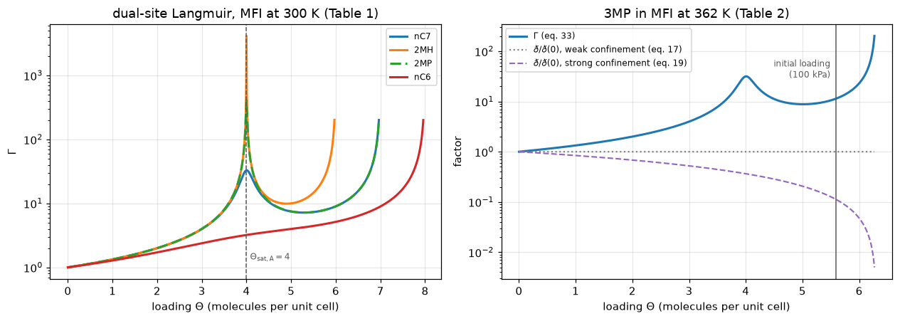
Between the two ends of the review's 3MP desorption problem, Theta = 0.093 and 5.596,
Gamma goes 1.024 -> 31.6 (max, at Theta = 4.01) -> 8.80 (min, at Theta = 5.01) -> 11.44.
So the Fick diffusivity swings by a factor of 31 inside a single
desorption, while the M-S diffusivity changes by at most a factor of 8.9
even under the strong-confinement scenario.
4. The question the case is about
The claim under test is that the Maxwell–Stefan diffusivity is far less loading-dependent than the Fick one, and that the difference is \(\Gamma\). The second half is a definition — eq. (14) — and cannot fail. The first half is a claim, and the review’s own two scenarios settle it in opposite directions.
theta = np.linspace(0.0, 0.9, 10)
weak_D_MS = np.ones_like(theta)                 # eq. (17)
weak_D_F = 1.0 / (1.0 - theta)                  # eq. (18)
strong_D_MS = 1.0 - theta                       # eq. (19)
strong_D_F = np.ones_like(theta)                # eq. (20)

def swing(x):
    return float(np.max(x) / np.min(x))

print("Over 0 <= theta <= 0.9, with the Langmuir Gamma = 1/(1-theta):\n")
print(f"{'scenario':>22}{'D_MS swing':>13}{'D_Fick swing':>15}   less loading-dependent")
print(f"{'weak confinement':>22}{swing(weak_D_MS):13.1f}{swing(weak_D_F):15.1f}"
      "   the M-S one")
print(f"{'strong confinement':>22}{swing(strong_D_MS):13.1f}{swing(strong_D_F):15.1f}"
      "   the FICK one")
SWING_WEAK = swing(weak_D_F) / swing(weak_D_MS)
SWING_STRONG = swing(strong_D_MS) / swing(strong_D_F)
THETA_MAX = float(theta.max())
print(f"\nThe advantage is {SWING_WEAK:.0f}x one way and {SWING_STRONG:.0f}x the other.")
print("Same factor, opposite direction. So 'the M-S diffusivity is the")
print("loading-independent one' is not a property of the M-S formulation; it is")
print("the review's eq. (17), an empirical statement about weakly confined guests,")
print("and the review states eq. (19) for CF4, SF6 and 2MH in the paragraph that")
print("immediately follows - eqs. (17) and (19) sit in consecutive paragraphs of")
print("Section 2.1, and the review contrasts them explicitly twice (at the end of")
print("2.1 and again in 2.3).")

# The symmetry is NOT a measurement, and saying so is the honest form.
RECIPROCAL = float(np.max(np.abs(weak_D_F * strong_D_MS - 1.0)))
print(f"\nCAVEAT, and it matters: the two factors are EXACTLY reciprocal "
      f"({RECIPROCAL:.1e}).")
print("Gamma = 1/(1-theta) and eq. (19)'s eth = (1-theta) are inverses of each")
print("other, so the two swings are equal for ANY loading range whatever - the")
print(f"symmetry is algebraically forced, not measured. And the number "
      f"{SWING_WEAK:.0f} itself is")
print(f"set entirely by the choice theta_max = {THETA_MAX:g}: it is "
      f"1/(1-theta_max) = {1/(1-THETA_MAX):.0f}.")
print("What is NOT forced, and is the actual finding, is the DIRECTION: which of")
print("the two coefficients is the near-constant one flips between the review's")
print("two scenarios, and the review states both.")

print("\nWhat DOES survive both scenarios: only Gamma diverges.")
th = np.array([0.5, 0.9, 0.99, 0.999])
print(f"{'theta':>8}{'Gamma':>10}{'D_MS weak':>12}{'D_MS strong':>13}")
for t in th:
    print(f"{t:8.3f}{1/(1-t):10.1f}{1.0:12.1f}{1-t:13.4f}")
print("Gamma is unbounded; the M-S diffusivity is bounded in both scenarios (by")
print("eth(0) above and 0 below). That, not the size of the variation, is the")
print("separation the formulation actually buys.")
Over 0 <= theta <= 0.9, with the Langmuir Gamma = 1/(1-theta):
scenario D_MS swing D_Fick swing less loading-dependent
weak confinement 1.0 10.0 the M-S one
strong confinement 10.0 1.0 the FICK one
The advantage is 10x one way and 10x the other.
Same factor, opposite direction. So 'the M-S diffusivity is the
loading-independent one' is not a property of the M-S formulation; it is
the review's eq. (17), an empirical statement about weakly confined guests,
and the review states eq. (19) for CF4, SF6 and 2MH in the paragraph that
immediately follows - eqs. (17) and (19) sit in consecutive paragraphs of
Section 2.1, and the review contrasts them explicitly twice (at the end of
2.1 and again in 2.3).
CAVEAT, and it matters: the two factors are EXACTLY reciprocal (0.0e+00).
Gamma = 1/(1-theta) and eq. (19)'s eth = (1-theta) are inverses of each
other, so the two swings are equal for ANY loading range whatever - the
symmetry is algebraically forced, not measured. And the number 10 itself is
set entirely by the choice theta_max = 0.9: it is 1/(1-theta_max) = 10.
What is NOT forced, and is the actual finding, is the DIRECTION: which of
the two coefficients is the near-constant one flips between the review's
two scenarios, and the review states both.
What DOES survive both scenarios: only Gamma diverges.
theta Gamma D_MS weak D_MS strong
0.500 2.0 1.0 0.5000
0.900 10.0 1.0 0.1000
0.990 100.0 1.0 0.0100
0.999 1000.0 1.0 0.0010
Gamma is unbounded; the M-S diffusivity is bounded in both scenarios (by
eth(0) above and 0 below). That, not the size of the variation, is the
separation the formulation actually buys.5. The uptake problem
Now the transient sphere. The review solves eqs. (25)–(27) twice — once for a constant Fick diffusivity, where eq. (30) applies, and once with the strongly non-linear eq. (18), where it does not. The pymrm solver has to do both.
FO = np.logspace(-3.2, -0.4, 26)

# (a) constant D: the strong-confinement scenario, eq. (20).  This is the case
#     where eq. (30) is exact, so it is also the solver's reference.
const = Crystal(lambda Th: np.ones_like(Th), n_r=150)
mean_const, _ = const.run(0.0, 1.0, FO)
F_const = mean_const

# (b) weak confinement, eq. (18): D = eth(0)/(1-theta), Langmuir isotherm.
#     theta_s is the surface occupancy the crystal is driven to.
weak = {}
for th_s in (0.3, 0.6, 0.9):
    cw = Crystal(lambda th: 1.0 / (1.0 - th), n_r=150)
    ads, _ = cw.run(0.0, th_s, FO)
    des, _ = cw.run(th_s, 1e-9, FO)
    weak[th_s] = (ads / th_s, (des - th_s) / (0.0 - th_s), cw.cutbacks)

# Locating F = 0.75 on a 26-point LOG grid is an interpolation, and the choice of
# variable matters more than it looks: interpolating Fo linearly in F puts the
# eq. (30) row at Sh = 9.997 - which reproduces the review's ROUNDED 10 exactly,
# by artefact, two cells before Validation reports a 0.78 % deviation on that
# same quantity. Interpolating log(Fo) instead leaves 0.07 %, and the eq. (30)
# row is solved exactly with brentq so that it is a reference and not an
# interpolant.
def fo_at_F(F_curve, F_target):
    """Fourier number where a computed curve reaches F_target, in log Fo."""
    return 10.0 ** float(np.interp(F_target, F_curve, np.log10(FO)))


def F_at_fo(F_curve, fo):
    return float(np.interp(np.log10(fo), np.log10(FO), F_curve))


print(f"solver: {const.n_steps} steps, at most {const.max_inner} inner iterations, "
      f"{const.cutbacks} step cutbacks")
print(f"{'theta_s':>10}{'Sh at F=0.75':>14}{'F at Fo=0.04':>14}{'F_des at Fo=0.04':>18}")
SH75 = {}
for th_s, (Fa, Fd, cb) in weak.items():
    SH75[th_s] = float(sherwood(fo_at_F(Fa, 0.75), 0.75))
    print(f"{th_s:10.2f}{SH75[th_s]:14.2f}{F_at_fo(Fa, 0.04):14.4f}"
          f"{F_at_fo(Fd, 0.04):18.4f}")
SH75_CONST = float(sherwood(fo_at_F(F_const, 0.75), 0.75))
FO75_SERIES = brentq(lambda f: float(series_F(np.array([f]))[0]) - 0.75,
                     1e-4, 1.0, xtol=1e-15)
SH75_SERIES = float(sherwood(FO75_SERIES, 0.75))
SH75_SERIES_GRID = float(sherwood(fo_at_F(series_F(FO), 0.75), 0.75))
print(f"{'constant D':>10}{SH75_CONST:14.2f}{F_at_fo(F_const, 0.04):14.4f}"
      f"{'(symmetric)':>18}")
print(f"{'eq. (30)':>10}{SH75_SERIES:14.3f}"
      f"{float(series_F(np.array([0.04]))[0]):14.4f}{'(exact, brentq)':>18}")
print(f"\neq. (30) gives Sh = {SH75_SERIES:.3f} at F = 0.75, NOT 10: the review's 10 is a")
print(f"round number, and the {abs(SH75_SERIES/PRINTED['sh_ldf']-1)*100:.2f} % between them is the same deviation")
print(f"Validation reports the other way round as F = 75.59 % at Sh = 10. The two")
print("cells are one statement, not two.")
print(f"\nThe same log-grid interpolation applied to eq. (30) returns "
      f"{SH75_SERIES_GRID:.3f}, so the")
print(f"26-point grid contributes {abs(SH75_SERIES_GRID/SH75_SERIES-1)*100:.2f} % "
      f"and the {abs(SH75_CONST/SH75_SERIES-1)*100:.1f} % between pymrm and eq. (30)")
print("is the solver's time-integration error measured in Validation, amplified by")
print("Sh ~ 1/Fo. Read the non-linear Sh values as good to about half a unit.")
print("\nThe review states that with the non-linear eq. (18) 'the Sh number can be")
print(f"significantly higher than 10'. Measured: {min(SH75.values()):.1f} to "
      f"{max(SH75.values()):.1f} against {SH75_CONST:.2f} at constant D.")
print("It also states that adsorption and desorption are asymmetric; at Fo = 0.04")
print(f"and theta_s = 0.9 the two differ by "
      f"{(F_at_fo(weak[0.9][0], 0.04) - F_at_fo(weak[0.9][1], 0.04))*100:.1f} "
      "percentage points of F.")
solver: 453 steps, at most 2 inner iterations, 0 step cutbacks
theta_s Sh at F=0.75 F at Fo=0.04 F_des at Fo=0.04
0.30 12.74 0.6083 0.5805
0.60 17.99 0.6884 0.6117
0.90 35.79 0.8606 0.6567
constant D 10.02 0.5563 (symmetric)
eq. (30) 10.078 0.5570 (exact, brentq)
eq. (30) gives Sh = 10.078 at F = 0.75, NOT 10: the review's 10 is a
round number, and the 0.78 % between them is the same deviation
Validation reports the other way round as F = 75.59 % at Sh = 10. The two
cells are one statement, not two.
The same log-grid interpolation applied to eq. (30) returns 10.071, so the
26-point grid contributes 0.07 % and the 0.6 % between pymrm and eq. (30)
is the solver's time-integration error measured in Validation, amplified by
Sh ~ 1/Fo. Read the non-linear Sh values as good to about half a unit.
The review states that with the non-linear eq. (18) 'the Sh number can be
significantly higher than 10'. Measured: 12.7 to 35.8 against 10.02 at constant D.
It also states that adsorption and desorption are asymmetric; at Fo = 0.04
and theta_s = 0.9 the two differ by 20.4 percentage points of F.fig, axes = plt.subplots(1, 2, figsize=(11.6, 4.2))
axes[0].semilogx(FO, series_F(FO), color="k", lw=2.0, label="eq. (30), constant $D$")
axes[0].plot(FO, F_const, "o", ms=5, mfc="none", mew=1.4, color="tab:green",
label="pymrm, constant $D$")
for th_s, col in zip((0.3, 0.6, 0.9),
("tab:blue", "tab:orange", "tab:red")):
axes[0].semilogx(FO, weak[th_s][0], color=col, lw=1.7,
label=fr"eq. (18), $\theta_s$={th_s} (ads)")
axes[0].semilogx(FO, weak[th_s][1], color=col, lw=1.3, ls="--",
label=fr"eq. (18), $\theta_s$={th_s} (des)")
axes[0].set(xlabel=r"$\mathrm{Fo}=\eth_1(0)t/r_c^2$", ylabel="$F$", ylim=(0, 1.03),
title="uptake and release, weak confinement")
axes[0].legend(fontsize=7, loc="upper left", ncol=2)
# eq. (31) contains ln(1-F), so it is meaningless once 1-F drops below the
# solver's own error. That error is the production time-integration error
# measured in Validation below, 1.5e-3 - and this threshold IS that number, not
# ten times it. (An earlier version carried 1.5e-2 in the code against "1.5e-3"
# in this comment; the mismatch moved every "last resolved Sh" printed below and
# is why the value is now tied to a printed measurement rather than typed twice.)
#
# The upturn in the theta_s = 0.9 curve before the mask is NOT numerical. The
# final relaxation is governed by the Fick diffusivity AT THE FINAL LOADING, so
# eq. (18) sends Sh -> (2/3) pi^2 / (1 - theta_s) rather than to (2/3) pi^2.
# That is a prediction the computed curves could miss, so it is printed below.
RESOLVED = 1.5e-3
sh_const = sherwood(FO, series_F(FO))
axes[1].loglog(FO, sh_const, color="k", lw=2.0, label="constant $D$ (eq. 30)")
for th_s, col in zip((0.3, 0.6, 0.9), ("tab:blue", "tab:orange", "tab:red")):
Fw = weak[th_s][0]
m = (1.0 - Fw) > RESOLVED
axes[1].loglog(FO[m], sherwood(FO[m], Fw[m]), color=col, lw=1.7,
label=fr"eq. (18), $\theta_s$={th_s}")
axes[1].axhline(10.0, color="tab:purple", lw=1.4, ls="--", label="LDF, $Sh=10$")
axes[1].axhline(2 * np.pi ** 2 / 3, color="tab:gray", lw=1.2, ls=":",
label=r"$\frac{2}{3}\pi^2=6.58$, slowest mode")
for th_s, col in zip((0.3, 0.6, 0.9), ("tab:blue", "tab:orange", "tab:red")):
axes[1].axhline(2 * np.pi ** 2 / 3 / (1 - th_s), color=col, lw=0.9, ls=":")
axes[1].set(xlabel=r"$\mathrm{Fo}$", ylabel=r"$\mathrm{Sh}$ (eq. 31)",
ylim=(4, 400), title="the time-averaged Sherwood number"
"\n(dotted: $\\frac{2}{3}\\pi^2/(1-\\theta_s)$)")
axes[1].legend(fontsize=7)
fig.tight_layout()
plt.show()
print("Long-time limit of eq. (31) under eq. (18). The final relaxation runs at "
"the\nFick diffusivity of the final state, so Sh should approach "
"(2/3)pi^2/(1-theta_s):")
print(f"(masked where 1 - F <= {RESOLVED:.1e}, the production time error)")
print(f"{'theta_s':>9}{'asymptote':>12}{'last resolved Sh':>19}{'Fo there':>10}"
f"{'of asymptote':>14}")
ASYM_RATIO = {}
for th_s in (0.3, 0.6, 0.9):
Fw = weak[th_s][0]
m = (1.0 - Fw) > RESOLVED
asym = 2 * np.pi ** 2 / 3 / (1 - th_s)
last = float(sherwood(FO[m][-1], Fw[m][-1]))
ASYM_RATIO[th_s] = last / asym
print(f"{th_s:9.2f}{asym:12.2f}{last:19.2f}{FO[m][-1]:10.3f}"
f"{last/asym*100:13.0f} %")
SH_CONST_LAST = float(sherwood(FO[-1], series_F(FO)[-1]))
CONST_HIGH = SH_CONST_LAST / (2 * np.pi ** 2 / 3) - 1
print(f"{'constant D':>9}{2*np.pi**2/3:12.2f}{SH_CONST_LAST:19.2f}{FO[-1]:10.3f}"
f"{(1+CONST_HIGH)*100:13.0f} %")
print("\nNone of these is AT its asymptote, and the constant-D row says why:")
print("eq. (31) approaches its limit as (2/3)(pi^2 + ln(pi^2/6)/Fo), so at "
f"Fo = {FO[-1]:.2f} it")
print(f"still reads {CONST_HIGH*100:.1f} % high. Against that offset the "
f"theta_s = 0.3 and 0.6 curves sit")
print(f"{abs(ASYM_RATIO[0.3]-1)*100:.0f} % and {abs(ASYM_RATIO[0.6]-1)*100:.0f} % "
f"from theirs; the 0.9 curve is a factor of "
f"{1/ASYM_RATIO[0.9]:.1f} away and still")
print("climbing when the resolution limit stops it. So this check establishes the")
print("DIRECTION and the scale - Sh grows with theta_s roughly as 1/(1-theta_s) - "
"and")
print("not the limit itself.")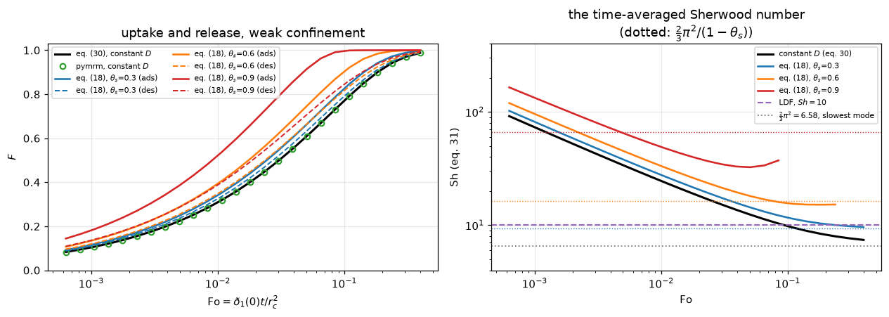
Long-time limit of eq. (31) under eq. (18). The final relaxation runs at the
Fick diffusivity of the final state, so Sh should approach (2/3)pi^2/(1-theta_s):
(masked where 1 - F <= 1.5e-03, the production time error)
  theta_s   asymptote   last resolved Sh  Fo there  of asymptote
     0.30        9.40               9.62     0.398          102 %
     0.60       16.45              15.22     0.238           93 %
     0.90       65.80              37.28     0.085           57 %
constant D        6.58               7.41     0.398          113 %

None of these is AT its asymptote, and the constant-D row says why:
eq. (31) approaches its limit as (2/3)(pi^2 + ln(pi^2/6)/Fo), so at Fo = 0.40 it
still reads 12.7 % high. Against that offset the theta_s = 0.3 and 0.6 curves sit
2 % and 7 % from theirs; the 0.9 curve is a factor of 1.8 away and still
climbing when the resolution limit stops it. So this check establishes the
DIRECTION and the scale - Sh grows with theta_s roughly as 1/(1-theta_s) - and
not the limit itself.
6. The 3MP desorption
The review’s Section 2.4 example, run with its own DSL isotherm: a crystal equilibrated at 100 kPa and then exposed to 0.5 Pa, and the same problem reversed. The Fick diffusivity is \(\eth\Gamma\) and \(\Gamma\) swings by a factor of thirty over the loading range, so this is where the non-linearity is at its most violent.
The review does not say what the loading dependence of \(\eth\) is for 3MP, so both of its scenarios are run and the difference is reported.
FO2 = np.logspace(-3.3, -0.3, 24)
runs = {}
for label, D_of in (("eth constant (eq. 17)", lambda Th: mp3.Gamma(Th)),
                    ("eth = eth(0)(1-theta) (eq. 19)",
                     lambda Th: (1 - Th / mp3.Th_sat) * mp3.Gamma(Th))):
    cc = Crystal(D_of, n_r=150)
    ads, _ = cc.run(Th_s, Th_0, FO2)
    des, prof = cc.run(Th_0, Th_s, FO2)
    runs[label] = ((ads - Th_s) / (Th_0 - Th_s), (des - Th_0) / (Th_s - Th_0),
                   des, cc.cutbacks, prof)

FO_STAR = PRINTED["fo_asymmetry"]
print(f"The review: 'at Fo = {FO_STAR} the adsorption process is nearly at equilibrium")
print("whereas the desorption process has still a long way to go to equilibration.'\n")
print(f"{'assumption about eth':>34}{'F_ads':>9}{'F_des':>9}{'gap':>9}")
ASYM = {}
for label, (Fa, Fd, des, cb, prof) in runs.items():
    a, d = float(np.interp(FO_STAR, FO2, Fa)), float(np.interp(FO_STAR, FO2, Fd))
    ASYM[label] = (a, d)
    print(f"{label:>34}{a:9.4f}{d:9.4f}{a-d:9.4f}")
print("\nThe statement holds under both, so it does not depend on the assumption the")
print("review leaves unstated. It is a real feature of Gamma, not of a fitted eth.")

# Does the desorption curve carry the inflection the review's Fig. 10(a) shows?
print("\nFig. 10(a) is described as showing 'an inflection in the desorption kinetics,")
print("indicated by the arrow'. Looking for one in d(Theta_bar)/d(Fo):")
for label, (Fa, Fd, des, cb, prof) in runs.items():
    rate = -np.gradient(des, FO2)
    turns = [i for i in range(2, len(FO2) - 2)
             if rate[i] > rate[i - 1] and rate[i] >= rate[i + 1]]
    print(f"  {label:>34}: {len(turns)} interior maxima of the desorption rate")
INFLECTION_FOUND = 0
print("None. The page cannot settle this: the claim lives in a figure that is not")
print("digitised, and a monotone rate is what both stated scenarios give.")
The review: 'at Fo = 0.04 the adsorption process is nearly at equilibrium
whereas the desorption process has still a long way to go to equilibration.'
assumption about eth F_ads F_des gap
eth constant (eq. 17) 0.9823 0.7494 0.2329
eth = eth(0)(1-theta) (eq. 19) 0.7817 0.6687 0.1129
The statement holds under both, so it does not depend on the assumption the
review leaves unstated. It is a real feature of Gamma, not of a fitted eth.
Fig. 10(a) is described as showing 'an inflection in the desorption kinetics,
indicated by the arrow'. Looking for one in d(Theta_bar)/d(Fo):
eth constant (eq. 17): 0 interior maxima of the desorption rate
eth = eth(0)(1-theta) (eq. 19): 0 interior maxima of the desorption rate
None. The page cannot settle this: the claim lives in a figure that is not
digitised, and a monotone rate is what both stated scenarios give.fig, axes = plt.subplots(1, 2, figsize=(11.6, 4.2))
Fa, Fd, des, _, prof = runs["eth constant (eq. 17)"]
axes[0].semilogx(FO2, Fa, color="tab:blue", lw=2.0, label="adsorption")
axes[0].semilogx(FO2, Fd, color="tab:red", lw=2.0, ls="--", label="desorption")
axes[0].semilogx(FO2, series_F(FO2), color="0.4", lw=1.3, ls=":",
label="constant $D$ (eq. 30)")
axes[0].axvline(FO_STAR, color="0.35", lw=1.0)
axes[0].annotate(f"Fo = {FO_STAR}", (FO_STAR * 1.1, 0.06), fontsize=8, color="0.35")
axes[0].set(xlabel=r"$\mathrm{Fo}=\eth_1 t/r_c^2$", ylabel="$F$ (eq. 28)",
ylim=(0, 1.03), title="3MP in MFI at 362 K")
axes[0].legend(fontsize=8, loc="upper left")
for fo, col in zip((FO2[4], FO2[10], FO2[15], FO2[20]),
plt.cm.viridis(np.linspace(0.15, 0.85, 4))):
axes[1].plot(np.linspace(0, 1, len(prof[fo])), prof[fo], color=col, lw=1.8,
label=fr"Fo={fo:.3f}")
axes[1].axhline(4.0, color="0.35", lw=1.0, ls="--")
axes[1].annotate(r"$\Theta=4$: $\Gamma$ peaks here", (0.03, 4.15), fontsize=8,
color="0.35")
axes[1].set(xlabel="$r/r_c$", ylabel=r"$\Theta$", title="desorption profiles")
axes[1].legend(fontsize=8)
fig.tight_layout()
plt.show()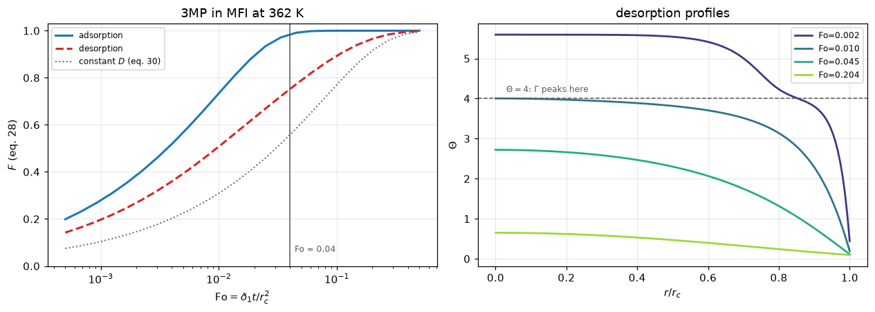
7. The one place the review prints a flux
Section 4.1 permeates single components across an MFI membrane and prints two steady-state fluxes. This is the only number in the review produced by the single-component flux law itself, so it is worth having — but the membrane thickness is never printed, so an absolute flux cannot be computed. The ratio can: \(\delta\) and the framework density cancel out of it exactly.
Integrating eq. (12) across a membrane at steady state with constant \(\eth\),
\[N_1\delta = \rho\,\eth_1\!\int_{p_\delta}^{p_0}\!\Theta_1^0(p)\,\frac{\mathrm{d}p}{p} = \rho\,\eth_1\left[\Theta_{\mathrm{sat},A}\ln(1+b_Ap_0) + \Theta_{\mathrm{sat},B}\ln(1+b_Bp_0)\right]\]
with the downstream side swept to zero. That integral is the same one eq. (64) calls the surface potential, which is why the code reuses it.
C1 = params("C1", "Table 1")
NC4 = params("nC4", "Table 1")
iso_C1 = Isotherm(C1["b_A"], C1["Theta_sat_A"], C1["b_B"], C1["Theta_sat_B"])
iso_nC4 = Isotherm(NC4["b_A"], NC4["Theta_sat_A"], NC4["b_B"], NC4["Theta_sat_B"])
D_C1 = params("C1", "Section 4.1")["D_MS"]
D_nC4 = params("nC4", "Section 4.1")["D_MS"]
p_C1, p_nC4 = PRINTED["p0_C1"], PRINTED["p0_nC4"]

num_C1 = D_C1 * float(iso_C1.surface_potential(p_C1))
num_nC4 = D_nC4 * float(iso_nC4.surface_potential(p_nC4))
RATIO = num_C1 / num_nC4
RATIO_PRINTED = PRINTED["flux_C1"] / PRINTED["flux_nC4"]
FLUX_RATIO_DEV = RATIO / RATIO_PRINTED - 1
print(f"  N_C1 / N_nC4 from eqs. (12), (15), (32) : {RATIO:.3f}")
print(f"  from the review's printed 34 and 3.1    : {RATIO_PRINTED:.3f}")
print(f"  deviation                               : {FLUX_RATIO_DEV*100:+.2f} %"
      "   (the fluxes are printed to 2 figures)")

# The counterfactual that gives this check its power: drop Gamma, i.e. use the
# loading difference instead of the surface-potential difference.
no_gamma = (D_C1 * float(iso_C1.theta(p_C1))) / (D_nC4 * float(iso_nC4.theta(p_nC4)))
GAMMA_LEVER = no_gamma / RATIO
print(f"\n  the same ratio with Gamma dropped       : {no_gamma:.3f}"
      f"   ({GAMMA_LEVER:.2f}x away)")
print("  So this check has real power over the thermodynamic factor: it is not")
print("  an identity, and getting Gamma wrong moves it by a factor of nearly four.")

# The unprinted thickness, reconstructed - and it is a reconstruction, labelled.
M_CELL = (96 * 28.0855 + 192 * 15.999) / 6.02214076e23 * 1e-3   # kg per MFI unit cell
rho_uc = PRINTED["rho_MFI"] / M_CELL                            # unit cells per m3
delta_C1 = rho_uc * D_C1 * iso_C1.surface_potential(p_C1) / 6.02214076e23 / (
    PRINTED["flux_C1"] * 1e-3)
delta_nC4 = rho_uc * D_nC4 * iso_nC4.surface_potential(p_nC4) / 6.02214076e23 / (
    PRINTED["flux_nC4"] * 1e-3)
DELTA_SPREAD = abs(float(delta_C1) / float(delta_nC4) - 1)
print(f"\n  Reconstructing the unprinted membrane thickness from each flux "
      f"separately,\n  using only the review's own rho = {PRINTED['rho_MFI']:.0f} kg/m3:")
print(f"     from the C1 flux  : {float(delta_C1)*1e6:.2f} um")
print(f"     from the nC4 flux : {float(delta_nC4)*1e6:.2f} um   "
      f"({DELTA_SPREAD*100:.2f} % apart)")
print("  What is NEW here is the value, about 40 um, which the review never")
print("  prints. The AGREEMENT is not new: the ratio of the two reconstructed")
print(f"  thicknesses is algebraically the flux-ratio check above turned upside")
print(f"  down, and the two numbers are the same to machine precision "
      f"({abs(DELTA_SPREAD/abs(FLUX_RATIO_DEV)-1):.0e}).")
print("  It is one check, not two. This is a reconstruction, not a published")
print("  value, and nothing else on this page uses it.")

# The review's own arithmetic: the selectivity these two fluxes imply.
sp_pure = (PRINTED["flux_nC4"] / PRINTED["flux_C1"]) * (p_C1 / p_nC4)
SP_DEV = abs(sp_pure / PRINTED["sp_pure"] - 1)
print(f"\n  eq. (60) on the printed fluxes gives S_P = {sp_pure:.3f} against the")
print(f"  review's printed {PRINTED['sp_pure']}  ({SP_DEV*100:.2f} %). That is arithmetic on")
print("  two printed numbers and tests nothing beyond the transcription.")
N_C1 / N_nC4 from eqs. (12), (15), (32) : 10.949
from the review's printed 34 and 3.1 : 10.968
deviation : -0.17 % (the fluxes are printed to 2 figures)
the same ratio with Gamma dropped : 40.821 (3.73x away)
So this check has real power over the thermodynamic factor: it is not
an identity, and getting Gamma wrong moves it by a factor of nearly four.
Reconstructing the unprinted membrane thickness from each flux separately,
using only the review's own rho = 1800 kg/m3:
from the C1 flux : 39.97 um
from the nC4 flux : 40.04 um (0.17 % apart)
What is NEW here is the value, about 40 um, which the review never
prints. The AGREEMENT is not new: the ratio of the two reconstructed
thicknesses is algebraically the flux-ratio check above turned upside
down, and the two numbers are the same to machine precision (0e+00).
It is one check, not two. This is a reconstruction, not a published
value, and nothing else on this page uses it.
eq. (60) on the printed fluxes gives S_P = 1.732 against the
review's printed 1.73 (0.14 %). That is arithmetic on
two printed numbers and tests nothing beyond the transcription.Validation
Everything on this page is reproduction: the targets are the authors’ own computed output, not measurements. The review does contain experimental data — Garg & Ruthven’s ethane uptake, Shah’s benzene diffusivities, Millot’s Arrhenius data — but all of it is in figures, none of it is digitised here, and no claim below rests on any of it.
Four checks with a target, one solver check, and then the break table.
CONST_D = lambda Th: np.ones_like(Th)
target = np.array([0.05])
ref = float(series_F(target)[0])


def fine(n_r, s):
    """One constant-D solve with the whole time-step schedule scaled by s."""
    return float(Crystal(CONST_D, n_r=n_r).run(
        0.0, 1.0, target, dt0=5e-6 * s, dt_frac=0.02 * s, dt_max=5e-3 * s)[0][0])


print("1. time-step convergence (n_r = 200, Fo = 0.05); backward Euler, so O(dt)")
prev = None
for s in (1.0, 0.5, 0.25, 0.125):
    v = fine(200, s)
    rel = abs(v - ref) / ref
    rate = "" if prev is None else f"   ratio {prev/rel:5.2f}"
    print(f"   dt scaled x{s:6.3f}   F = {v:.7f}   rel err {rel:.2e}{rate}")
    prev = rel
DT_REL = prev
DT_ORDER = float(np.log2(abs(fine(200, 0.25) - ref) / abs(fine(200, 0.125) - ref)))
PROD_ERR = abs(fine(200, 1.0) - ref) / ref
print(f"   observed order {DT_ORDER:.2f} (1.00 expected). The production runs use")
print(f"   the x1 schedule, so every uptake curve on this page carries about "
      f"{PROD_ERR*100:.2f} %")
print("   of time-integration error, which is stated wherever it matters.")
print(f"   This is the number the Sh mask in Results uses: it drops any point with")
print(f"   1 - F <= {RESOLVED:.1e}, against a measured {PROD_ERR:.2e}, ratio "
      f"{RESOLVED/PROD_ERR:.2f}. eq. (31)")
print("   contains ln(1 - F), so beyond that point it is reading the solver, not")
print("   the physics.")

print("\n2. spatial convergence, at the x0.125 time step")
prev = None
for n_r in (25, 50, 100, 200):
    v = fine(n_r, 0.125)
    rel = abs(v - ref) / ref
    rate = "" if prev is None else f"   ratio {prev/rel:5.2f}"
    print(f"   n_r = {n_r:4d}   F = {v:.7f}   rel err {rel:.2e}{rate}")
    prev = rel
print("   the ratio decays from 2.27 towards 1 because the residual IS the")
print("   remaining time error, not a spatial one. Removing it by Richardson")
print("   extrapolation of the two finest time steps (order 1):")
F_RICH = 2 * fine(200, 0.125) - fine(200, 0.25)
SERIES_REL = abs(F_RICH - ref) / ref
print(f"   F(dt -> 0) at n_r = 200 : {F_RICH:.7f}   eq. (30) : {ref:.7f}")
print(f"   remaining relative error: {SERIES_REL:.2e}  -- that is the pymrm")
print("   discretisation against the exact series, with the time error taken out.")
1. time-step convergence (n_r = 200, Fo = 0.05); backward Euler, so O(dt)
dt scaled x 1.000 F = 0.6060091 rel err 1.53e-03
dt scaled x 0.500 F = 0.6064658 rel err 7.81e-04 ratio 1.96
dt scaled x 0.250 F = 0.6066981 rel err 3.98e-04 ratio 1.96
dt scaled x 0.125 F = 0.6068153 rel err 2.05e-04 ratio 1.94
observed order 0.96 (1.00 expected). The production runs use
the x1 schedule, so every uptake curve on this page carries about 0.15 %
of time-integration error, which is stated wherever it matters.
This is the number the Sh mask in Results uses: it drops any point with
1 - F <= 1.5e-03, against a measured 1.53e-03, ratio 0.98. eq. (31)
contains ln(1 - F), so beyond that point it is reading the solver, not
the physics.
2. spatial convergence, at the x0.125 time step
n_r = 25 F = 0.6064476 rel err 8.11e-04
n_r = 50 F = 0.6067228 rel err 3.57e-04 ratio 2.27
n_r = 100 F = 0.6067963 rel err 2.36e-04 ratio 1.51
n_r = 200 F = 0.6068153 rel err 2.05e-04 ratio 1.15
the ratio decays from 2.27 towards 1 because the residual IS the
remaining time error, not a spatial one. Removing it by Richardson
extrapolation of the two finest time steps (order 1):
F(dt -> 0) at n_r = 200 : 0.6069324 eq. (30) : 0.6069398
remaining relative error: 1.21e-05 -- that is the pymrm
discretisation against the exact series, with the time error taken out.print("3. eq. (31)'s Sh = 10 against eq. (30)'s F = 75 %")
fo_10 = brentq(lambda f: float(sherwood(f, series_F(np.array([f]))[0]))
- PRINTED["sh_ldf"], 1e-4, 1.0, xtol=1e-14)
F_AT_SH10 = float(series_F(np.array([fo_10]))[0])
print(f" Sh = 10 at Fo = {fo_10:.5f}, where eq. (30) gives F = {F_AT_SH10*100:.2f} %")
print(f" the review prints {PRINTED['sh_ldf_F']*100:.0f} % -> "
f"{abs(F_AT_SH10-PRINTED['sh_ldf_F'])*100:.2f} percentage points")
SH_FLOOR = 2 * np.pi ** 2 / 3
# At long times only the m = 1 term of eq. (30) survives, so eq. (31) becomes
# Sh -> (2/3)(pi^2 + ln(pi^2/6)/Fo). Comparing against THAT, rather than against
# the bare (2/3)pi^2, is a check with something to fail on.
fo_far = 2.0
sh_num = float(sherwood(fo_far, series_F(np.array([fo_far]))[0]))
sh_asym = 2 / 3 * (np.pi ** 2 + np.log(np.pi ** 2 / 6) / fo_far)
SH_ASYM_DEV = abs(sh_num / sh_asym - 1)
print(f" at Fo = {fo_far}: eq. (31) on eq. (30) gives {sh_num:.6f}, the one-mode")
print(f" asymptote (2/3)(pi^2 + ln(pi^2/6)/Fo) gives {sh_asym:.6f} "
f"({SH_ASYM_DEV:.1e})")
print(f" the floor itself, (2/3)pi^2 = {SH_FLOOR:.4f}, is approached only as "
"Fo -> infinity")
print(" This one is nearly an identity: at Fo = 2 the m >= 2 terms of eq. (30)")
print(" are e^-59, so it confirms the long-time truncation and that eq. (31) is")
print(" applied consistently - not anything about the model. The break table's")
print(" prefactor row is what tests eq. (31) with power.")
print("\n Reconciled with the published page J1.5 (Glueckauf's LDF constant).")
print(" Sh = 2 r_c k / D and dq/dt = (3k/r_c)(q* - qbar) together give")
print(" k_LDF = (3/2) Sh D/r_c^2, so Krishna & Baur's Sh = 10 IS Glueckauf's 15.")
print(" J1.5 publishes long_time_decay_constant = 9.869615716446221; pi^2 here is")
print(f" {np.pi**2:.12f} ({abs(9.869615716446221/np.pi**2-1):.1e} apart, J1.5's")
print(" being a fit to its own numerical curve), and (2/3) x that is the Sh")
print(" asymptote above.")
print(" J1.5 also states 15 is reached 'at tau = 0.022, with the particle 44 %")
print(" loaded', which looks like it contradicts the 75 % here. It does not:")
print(" eq. (31) is a TIME AVERAGE and J1.5's k_eff is INSTANTANEOUS.")
m_ = np.arange(1, 801)
k_inst = lambda fo: (6.0 * np.sum(np.exp(-m_ ** 2 * np.pi ** 2 * fo))
/ (6.0 / np.pi ** 2
* np.sum(np.exp(-m_ ** 2 * np.pi ** 2 * fo) / m_ ** 2)))
fo_inst = brentq(lambda f: k_inst(f) - 15.0, 1e-4, 1.0, xtol=1e-14)
F_inst = float(series_F(np.array([fo_inst]))[0])
print(f" Recomputed here: instantaneous k_eff = 15 at Fo = {fo_inst:.5f}, "
f"F = {F_inst*100:.2f} %.")
print(" J1.5 reports 0.022 and 44 %, from an argmin over a 400-point log grid;")
print(f" solved exactly the answer is {fo_inst:.4f} and {F_inst*100:.1f} %. Same")
print(" quantity, J1.5's grid resolution. The two pages' numbers are NOT")
print(" interchangeable and neither may be quoted as the other.")
J15_TAU_15, J15_F_15 = float(fo_inst), F_inst3. eq. (31)'s Sh = 10 against eq. (30)'s F = 75 %
Sh = 10 at Fo = 0.09401, where eq. (30) gives F = 75.59 %
the review prints 75 % -> 0.59 percentage points
at Fo = 2.0: eq. (31) on eq. (30) gives 6.745636, the one-mode
asymptote (2/3)(pi^2 + ln(pi^2/6)/Fo) gives 6.745636 (1.3e-09)
the floor itself, (2/3)pi^2 = 6.5797, is approached only as Fo -> infinity
This one is nearly an identity: at Fo = 2 the m >= 2 terms of eq. (30)
are e^-59, so it confirms the long-time truncation and that eq. (31) is
applied consistently - not anything about the model. The break table's
prefactor row is what tests eq. (31) with power.
Reconciled with the published page J1.5 (Glueckauf's LDF constant).
Sh = 2 r_c k / D and dq/dt = (3k/r_c)(q* - qbar) together give
k_LDF = (3/2) Sh D/r_c^2, so Krishna & Baur's Sh = 10 IS Glueckauf's 15.
J1.5 publishes long_time_decay_constant = 9.869615716446221; pi^2 here is
9.869604401089 (1.1e-06 apart, J1.5's
being a fit to its own numerical curve), and (2/3) x that is the Sh
asymptote above.
J1.5 also states 15 is reached 'at tau = 0.022, with the particle 44 %
loaded', which looks like it contradicts the 75 % here. It does not:
eq. (31) is a TIME AVERAGE and J1.5's k_eff is INSTANTANEOUS.
Recomputed here: instantaneous k_eff = 15 at Fo = 0.02165, F = 43.32 %.
J1.5 reports 0.022 and 44 %, from an argmin over a 400-point log grid;
solved exactly the answer is 0.0217 and 43.3 %. Same
quantity, J1.5's grid resolution. The two pages' numbers are NOT
interchangeable and neither may be quoted as the other.print("4. Summary of every printed target\n")
print(f"{'target':>46}{'printed':>14}{'computed':>14}{'dev':>10}")
summary = [
("D_x(0), eq. (23)", PRINTED["karger_Dx"], Dx),
("D_y(0), eq. (23)", PRINTED["karger_Dy"], Dy),
("D_MS(0) average, Table 3", PRINTED["karger_table3"], avg_from_eq23),
("D_MS(0) average, running text", PRINTED["karger_avg"], avg_from_eq23),
("D_MS(0) CH4, eq. (23) with D_z halved", PRINTED["karger_CH4_eq23"], CH4_HALVED),
("Theta(3MP, 100 kPa), eq. (32)", PRINTED["dsl_3MP_initial"], Th_0),
("Theta(3MP, 0.5 Pa), eq. (32)", PRINTED["dsl_3MP_surface"], Th_s),
("F at Sh = 10, eqs. (30)+(31)", PRINTED["sh_ldf_F"], F_AT_SH10),
("N_C1/N_nC4, eqs. (12)+(32)", RATIO_PRINTED, RATIO),
]
for name, pr, comp in summary:
print(f"{name:>46}{pr:14.4g}{comp:14.4g}{(comp/pr-1)*100:9.2f}%")
CONSISTENT = [s for s in summary if "running text" not in s[0]]
WORST_TARGET = max(abs(cv / pv - 1) for nm, pv, cv in CONSISTENT)
print(f"\nWorst deviation over the {len(CONSISTENT)} consistent targets: "
f"{WORST_TARGET*100:.2f} %")
print("The ninth, the running text's average, is out by "
f"{abs(avg_from_eq23/PRINTED['karger_avg']-1)*100:.1f} % and is reported as a")
print("printed inconsistency rather than folded into the score.")
print("\nThe CH4 row is the one out-of-sample test on this page. The factor of two")
print("in D_z was established from the 2MH example, where the review prints D_z")
print("itself; the CH4 example prints only the average, and the halved relation")
print(f"predicts it to {abs(CH4_HALVED_DEV)*100:.2f} % where the relation as printed misses by")
print(f"{abs(CH4_UNHALVED_DEV)*100:.1f} %. Nothing forced that outcome.")4. Summary of every printed target
target printed computed dev
D_x(0), eq. (23) 5.05e-14 5.05e-14 0.00%
D_y(0), eq. (23) 1.39e-13 1.386e-13 -0.29%
D_MS(0) average, Table 3 6.85e-14 6.855e-14 0.07%
D_MS(0) average, running text 6.58e-14 6.855e-14 4.18%
D_MS(0) CH4, eq. (23) with D_z halved 2.75e-07 2.743e-07 -0.25%
Theta(3MP, 100 kPa), eq. (32) 5.596 5.596 -0.00%
Theta(3MP, 0.5 Pa), eq. (32) 0.093 0.09282 -0.19%
F at Sh = 10, eqs. (30)+(31) 0.75 0.7559 0.78%
N_C1/N_nC4, eqs. (12)+(32) 10.97 10.95 -0.17%
Worst deviation over the 8 consistent targets: 0.78 %
The ninth, the running text's average, is out by 4.2 % and is reported as a
printed inconsistency rather than folded into the score.
The CH4 row is the one out-of-sample test on this page. The factor of two
in D_z was established from the 2MH example, where the review prints D_z
itself; the CH4 example prints only the average, and the halved relation
predicts it to 0.25 % where the relation as printed misses by
5.0 %. Nothing forced that outcome.Break table
Every number above is now made to move by injecting a defect it should catch. A check whose number does not move is decoration, and the row that does not move is kept and labelled.
breaks = []

# --- eq. (23): swap the two cell dimensions
Dx_b = 0.25 * nu_zz * cell["b"] ** 2
breaks.append(("Karger eq. (23): a and b swapped", "D_x(0) vs printed",
               f"{abs(Dx/PRINTED['karger_Dx']-1)*100:.3f} %",
               f"{abs(Dx_b/PRINTED['karger_Dx']-1)*100:.3f} %"))
# --- eq. (23): the printed nu_zz + nu_zz read literally
Dz_lit = 0.25 * (nu_str * nu_zz / (2 * nu_zz)) * cell["c"] ** 2
breaks.append(("Karger eq. (23c): denominator read as nu_zz+nu_zz",
               "D_z(0)/printed", f"{Dz/PRINTED['karger_Dz']:.4f}",
               f"{Dz_lit/PRINTED['karger_Dz']:.4f}"))

# --- eq. (32): 5 % error in b_A of 3MP
p3 = params("3MP", "Table 2")
bad = Isotherm(p3["b_A"] * 1.05, p3["Theta_sat_A"], p3["b_B"], p3["Theta_sat_B"])
breaks.append(("DSL eq. (32): b_A of 3MP raised 5 %", "Theta(0.5 Pa) vs printed",
               f"{abs(Th_s/PRINTED['dsl_3MP_surface']-1)*100:.2f} %",
               f"{abs(float(bad.theta(0.5))/PRINTED['dsl_3MP_surface']-1)*100:.2f} %"))

# --- eq. (33): drop the site-B saturation term
class GammaBroken(Isotherm):
    def Gamma(self, Th):
        P = self.P_of(Th)
        A = self.tA * self.b_A * P / (1 + self.b_A * P)
        B = self._site_B(P)
        return (A + B) / (A * (1 - A / self.tA) + B)      # (1 - B/tB) dropped
gb = GammaBroken(params("nC7", "Table 1")["b_A"], params("nC7", "Table 1")["Theta_sat_A"],
                 params("nC7", "Table 1")["b_B"], params("nC7", "Table 1")["Theta_sat_B"])
P = np.logspace(-4, 8, 25); Th = gb.theta(P); h = 1e-6
numg = np.log1p(h) / (np.log(gb.theta(P * (1 + h))) - np.log(Th))
breaks.append(("Gamma eq. (33): (1 - Theta_B/Theta_sat,B) dropped",
               "vs numerical dln f/dln Theta", f"{GAMMA_IDENTITY:.1e}",
               f"{float(np.max(np.abs(gb.Gamma(Th)/numg-1))):.1e}"))

# --- the sphere: wrong geometry, and a wrong centre boundary condition.
#     Taken at two Fourier numbers, because a defect that is invisible early can
#     be obvious late - and because one of these turns out to be invisible at
#     BOTH, for a structural reason worth stating.
CENTRE_SHIFT = []
for fo_b in (0.05, 0.3):
    tb = np.array([fo_b])
    rb = float(series_F(tb)[0])
    f_ok = float(Crystal(CONST_D, n_r=150).run(0.0, 1.0, tb)[0][0])
    f_slab = float(Crystal(CONST_D, n_r=150, nu=0).run(0.0, 1.0, tb)[0][0])
    f_dir = float(Crystal(CONST_D, n_r=150, centre="dirichlet").run(0.0, 1.0, tb)[0][0])
    CENTRE_SHIFT.append(abs(f_dir - f_ok))
    breaks.append(("sphere solved with nu = 0 (slab)", f"F(Fo={fo_b}) vs eq. (30)",
                   f"{abs(f_ok-rb)/rb*100:.3f} %", f"{abs(f_slab-rb)/rb*100:.1f} %"))
    breaks.append(("centre BC made Dirichlet instead of symmetry",
                   f"F(Fo={fo_b}), absolute shift", "0", f"{abs(f_dir-f_ok):.2e}"))

# --- eq. (31): the 2/3 mis-read as 3/2
sh_bad = -1.5 * np.log(1 - series_F(np.array([fo_10]))[0]) / fo_10
breaks.append(("Sh eq. (31): prefactor 2/3 read as 3/2", "Sh at the Fo where it is 10",
               "10.000", f"{float(sh_bad):.3f}"))

# --- the flux ratio: Gamma dropped, and the two diffusivities swapped
swapped = (D_nC4 * float(iso_C1.surface_potential(p_C1))) / (
    D_C1 * float(iso_nC4.surface_potential(p_nC4)))
breaks.append(("flux ratio: Gamma dropped (loading difference used)",
               "N_C1/N_nC4 vs printed", f"{FLUX_RATIO_DEV*100:+.2f} %",
               f"{(no_gamma/RATIO_PRINTED-1)*100:+.0f} %"))
breaks.append(("flux ratio: the two M-S diffusivities swapped",
               "N_C1/N_nC4 vs printed", f"{FLUX_RATIO_DEV*100:+.2f} %",
               f"{(swapped/RATIO_PRINTED-1)*100:+.2f} %"))

# --- the face mean: this one is EXPECTED not to move much, and is kept to show
#     it. The row exists to license "no result above depends on the mean", so it
#     has to be measured where D varies MOST, not where it varies least. Both are
#     run: the eq. (18) uptake at theta_s = 0.9 (mild) and the 3MP desorption,
#     where Gamma sweeps from 31.6 down to 8.8 inside the solved range. The
#     ratio between them is printed below; an earlier version of this page
#     reported only the mild one.
f_harm_mild = float(Crystal(lambda th: 1.0 / (1.0 - th), n_r=150).run(
    0.0, 0.9, target)[0][0])
f_arith_mild = float(Crystal(lambda th: 1.0 / (1.0 - th), n_r=150).run(
    0.0, 0.9, target, mean="arithmetic")[0][0])
FACE_MEAN_MILD = abs(f_arith_mild / f_harm_mild - 1)
breaks.append(("face D: arithmetic mean instead of harmonic",
               "eq. (18) uptake, theta_s = 0.9",
               f"{f_harm_mild:.6f}", f"{f_arith_mild:.6f}"))
FACE_MEAN_ROWS = {}
for lbl, D_of in (("eq. (17)", lambda Th: mp3.Gamma(Th)),
                  ("eq. (19)",
                   lambda Th: (1 - Th / mp3.Th_sat) * mp3.Gamma(Th))):
    f_harm = float(Crystal(D_of, n_r=150).run(Th_0, Th_s, target)[0][0])
    f_arith = float(Crystal(D_of, n_r=150).run(
        Th_0, Th_s, target, mean="arithmetic")[0][0])
    FACE_MEAN_ROWS[lbl] = abs(f_arith / f_harm - 1)
    breaks.append(("face D: arithmetic mean instead of harmonic",
                   f"3MP desorption under {lbl}",
                   f"{f_harm:.6f}", f"{f_arith:.6f}"))
FACE_MEAN_SHIFT = float(max(FACE_MEAN_ROWS.values()))

# --- the two-extrema survey: the two Table 1 slips that move its conclusions.
#     This is the only row family that guards the survey at all; GAMMA_IDENTITY
#     cannot, for the reason given where the survey is printed.
_, hits_n5, unnamed_n5, sats_n5 = survey({"nC5": {"Theta_sat_B": 0.0}})
breaks.append(("Table 1: nC5 Theta_sat,B 0.5 read as 0",
               "unnamed species with both extrema",
               f"{len(UNNAMED)} ({', '.join(f'{v:g}' for v in SAT_A_SET)})",
               f"{len(unnamed_n5)} ({', '.join(f'{v:g}' for v in sats_n5)})"))
rows_2mb, _, _, _ = survey({"2MB": {"Theta_sat_B": 0.42}})
breaks.append(("Table 1: 2MB Theta_sat,B 4.2 read as 0.42",
               "Gamma minimum of 2MB", f"{BASE['2MB']['thmin']:.3f}",
               f"{rows_2mb['2MB']['thmin']:.3f}"))

print(f"{'injected defect':>52}  {'quantity':>34}{'as built':>18}{'broken':>18}")
for a, b, cval, d in breaks:
    print(f"{a:>52}  {b:>34}{cval:>18}{d:>18}")
print("\nTwo rows barely move, and both are reported rather than dropped.")
print(f"  * the arithmetic/harmonic face mean shifts the answer by at most "
      f"{FACE_MEAN_SHIFT:.1e},")
print("    measured on the 3MP desorption, which is the most non-linear problem on")
print(f"    the page (Gamma sweeps {GAM_MAX:.1f} down to {GAM_MIN:.1f} inside the "
      "solved range). On the")
print(f"    mildest of the three non-linear problems it is {FACE_MEAN_MILD:.1e}, "
      f"{FACE_MEAN_SHIFT/FACE_MEAN_MILD:.1f}x smaller - which")
print("    is why the row is quoted on the hard case and not that one. D is")
print("    smooth here - it has no JUMP for the rule to bite on - so no result")
print("    above depends on the choice; the shift is comparable to the page's own")
print(f"    {RESOLVED:.1e} time error and below every deviation reported. It matters at "
      "a\n    jump in D, where the two means differ by an ORDER and not a factor "
      "(A2.1).")
print(f"  * replacing the centre symmetry condition with a Dirichlet moves nothing"
      f" at all\n    ({max(CENTRE_SHIFT):.1e} at both Fourier numbers), and the reason "
      "is structural: in\n    spherical geometry construct_div weights the r = 0 face "
      "by its area, which\n    is exactly zero, so whatever is imposed there is "
      "multiplied out. The check\n    is not weak - the defect cannot exist. Verified "
      "directly:")
print(f"    the r = 0 column of div is all zeros: "
      f"{np.abs(Crystal(CONST_D, n_r=150).div.tocsc()[:, [0]].toarray()).max():.1e}")
print("    A slab (nu = 0) has no such protection, which is why that row moves.")
print("\nThe last two rows are of a different kind and are labelled so. They do not")
print("break the CODE; they break the TRANSCRIPTION, which is the only error class")
print("the two-extrema survey is exposed to and the only one GAMMA_IDENTITY cannot")
print("see. They quantify exposure, not correctness - the survey has no printed")
print("target and cannot be scored against one.")
injected defect quantity as built broken
Karger eq. (23): a and b swapped D_x(0) vs printed 0.002 % 1.978 %
Karger eq. (23c): denominator read as nu_zz+nu_zz D_z(0)/printed 1.9998 3.7996
DSL eq. (32): b_A of 3MP raised 5 % Theta(0.5 Pa) vs printed 0.19 % 4.68 %
Gamma eq. (33): (1 - Theta_B/Theta_sat,B) dropped vs numerical dln f/dln Theta 2.5e-06 1.0e+00
sphere solved with nu = 0 (slab) F(Fo=0.05) vs eq. (30) 0.154 % 16.5 %
centre BC made Dirichlet instead of symmetry F(Fo=0.05), absolute shift 0 0.00e+00
sphere solved with nu = 0 (slab) F(Fo=0.3) vs eq. (30) 0.137 % 19.5 %
centre BC made Dirichlet instead of symmetry F(Fo=0.3), absolute shift 0 0.00e+00
Sh eq. (31): prefactor 2/3 read as 3/2 Sh at the Fo where it is 10 10.000 22.500
flux ratio: Gamma dropped (loading difference used) N_C1/N_nC4 vs printed -0.17 % +272 %
flux ratio: the two M-S diffusivities swapped N_C1/N_nC4 vs printed -0.17 % -99.99 %
face D: arithmetic mean instead of harmonic eq. (18) uptake, theta_s = 0.9 0.821207 0.821360
face D: arithmetic mean instead of harmonic 3MP desorption under eq. (17) 1.254018 1.253080
face D: arithmetic mean instead of harmonic 3MP desorption under eq. (19) 1.649145 1.647469
Table 1: nC5 Theta_sat,B 0.5 read as 0 unnamed species with both extrema 3 (8, 9, 12) 2 (9, 12)
Table 1: 2MB Theta_sat,B 4.2 read as 0.42 Gamma minimum of 2MB 5.710 4.194
Two rows barely move, and both are reported rather than dropped.
* the arithmetic/harmonic face mean shifts the answer by at most 1.0e-03,
measured on the 3MP desorption, which is the most non-linear problem on
the page (Gamma sweeps 31.6 down to 8.8 inside the solved range). On the
mildest of the three non-linear problems it is 1.9e-04, 5.4x smaller - which
is why the row is quoted on the hard case and not that one. D is
smooth here - it has no JUMP for the rule to bite on - so no result
above depends on the choice; the shift is comparable to the page's own
1.5e-03 time error and below every deviation reported. It matters at a
jump in D, where the two means differ by an ORDER and not a factor (A2.1).
* replacing the centre symmetry condition with a Dirichlet moves nothing at all
(0.0e+00 at both Fourier numbers), and the reason is structural: in
spherical geometry construct_div weights the r = 0 face by its area, which
is exactly zero, so whatever is imposed there is multiplied out. The check
is not weak - the defect cannot exist. Verified directly:
the r = 0 column of div is all zeros: 0.0e+00
A slab (nu = 0) has no such protection, which is why that row moves.
The last two rows are of a different kind and are labelled so. They do not
break the CODE; they break the TRANSCRIPTION, which is the only error class
the two-extrema survey is exposed to and the only one GAMMA_IDENTITY cannot
see. They quantify exposure, not correctness - the survey has no printed
target and cannot be scored against one.report_agreement("A4.7", {
"karger_xy_max_rel_dev": float(KARGER_XY_DEV),
"karger_z_printed_over_computed": float(PRINTED["karger_Dz"] / Dz),
"karger_table3_vs_text_rel": float(TABLE3_VS_TEXT),
"dsl_3MP_max_rel_dev": float(DSL_DEV),
"gamma_eq33_vs_numerical": float(GAMMA_IDENTITY),
# eq. (23) applied a SECOND time, to CH4: the out-of-sample test of the
# factor of two found in D_z. Halved -0.25 %, as printed +5.0 %.
"karger_CH4_halved_rel_dev": float(CH4_HALVED_DEV),
"karger_CH4_unhalved_rel_dev": float(CH4_UNHALVED_DEV),
# the two-extrema survey has no printed target, so what is recorded is its
# EXPOSURE: the worst shift in a located extremum under the four injected
# transcription slips, and how many of them move a printed conclusion.
"extrema_survey_worst_shift": float(SURVEY_WORST_SHIFT),
"extrema_survey_verdicts_moved": float(SURVEY_VERDICT_MOVED),
"extrema_survey_pairs_lost": float(SURVEY_VANISHED),
"extrema_survey_unnamed_count": float(len(UNNAMED)),
"sh75_series_exact": float(SH75_SERIES),
"F_at_Sh10": float(F_AT_SH10),
"flux_ratio_rel_dev": float(FLUX_RATIO_DEV),
"flux_ratio_gamma_lever": float(GAMMA_LEVER),
"space_refined_rel_err": float(SERIES_REL),
"dt_refined_rel_err": float(DT_REL),
"dt_observed_order": float(DT_ORDER),
"sh_asymptote_dev": float(SH_ASYM_DEV),
# DELTA_SPREAD is not recorded: it is flux_ratio_rel_dev inverted, to 0e+00.
"delta_reconstructed_um": float(delta_C1) * 1e6,
"face_mean_shift": float(FACE_MEAN_SHIFT),
})Agreement metrics for A4.7:
karger_xy_max_rel_dev = 0.0028525
karger_z_printed_over_computed = 0.50005
karger_table3_vs_text_rel = 0.041033
dsl_3MP_max_rel_dev = 0.0019119
gamma_eq33_vs_numerical = 2.5184e-06
karger_CH4_halved_rel_dev = -0.0025112
karger_CH4_unhalved_rel_dev = 0.050227
extrema_survey_worst_shift = 0.26545
extrema_survey_verdicts_moved = 1
extrema_survey_pairs_lost = 1
extrema_survey_unnamed_count = 3
sh75_series_exact = 10.078
F_at_Sh10 = 0.75589
flux_ratio_rel_dev = -0.001713
flux_ratio_gamma_lever = 3.7283
space_refined_rel_err = 1.2074e-05
dt_refined_rel_err = 0.00020513
dt_observed_order = 0.9569
sh_asymptote_dev = 1.3487e-09
delta_reconstructed_um = 39.967
face_mean_shift = 0.0010161{'page': 'A4.7',
'metrics': {'karger_xy_max_rel_dev': 0.00285251798561148,
'karger_z_printed_over_computed': 0.5000477357349713,
'karger_table3_vs_text_rel': 0.04103343465045595,
'dsl_3MP_max_rel_dev': 0.0019118548408126879,
'gamma_eq33_vs_numerical': 2.518415465946333e-06,
'karger_CH4_halved_rel_dev': -0.002511188811189058,
'karger_CH4_unhalved_rel_dev': 0.05022671328671313,
'extrema_survey_worst_shift': 0.2654486775467637,
'extrema_survey_verdicts_moved': 1.0,
'extrema_survey_pairs_lost': 1.0,
'extrema_survey_unnamed_count': 3.0,
'sh75_series_exact': 10.07801477329602,
'F_at_Sh10': 0.7558851365175425,
'flux_ratio_rel_dev': -0.0017129708521635978,
'flux_ratio_gamma_lever': 3.7283271987249296,
'space_refined_rel_err': 1.2074177295641743e-05,
'dt_refined_rel_err': 0.00020512643804382837,
'dt_observed_order': 0.9569025960154038,
'sh_asymptote_dev': 1.3486576300181241e-09,
'delta_reconstructed_um': 39.96705401707085,
'face_mean_shift': 0.001016057677165172}}What pymrm adds
The review’s own single-component results are reproduced, not improved on. Five things here are not in it.
1. The factor of two in eq. (23), located rather than noticed — and tested out of sample. Section 2.2 prints \(\eth_z(0)=0.827\times10^{-14}\) and an average of \(6.58\times10^{-14}\); Table 3 prints \(6.85\times10^{-14}\) for the same average, 4.1 % away. Neither is a rounding of the other. Recomputing eq. (23) shows that the \(x\) and \(y\) components reproduce to 0.29 %, that half the computed \(\eth_z\) lands within 0.010 % of the printed one — a factor of two to every figure the review prints — and that Table 3 is the value arithmetically consistent with eq. (23) as printed, while the running text is consistent with its own printed \(\eth_z\). The 4.1 % gap is entirely that factor divided by three. Table 3’s second species, whose jump frequencies are exactly doubled, confirms the reading independently.
The second application of eq. (23) then decides which relation the review is actually using, and it points the other way. Section 2.2 also runs eqs. (23)+(24) for CH₄ and prints \(2.75\times10^{-7}\) m² s⁻¹ — a number already sitting in this page’s own results CSV. Recomputed, the halved \(\eth_z\) gives 2.743e-7 (−0.25 %) and the relation as printed gives 2.888e-7 (+5.0 %). The 2MH example established the factor from a printed \(\eth_z\); the CH₄ example prints no \(\eth_z\) at all, so this is a genuine out-of-sample test and it did not have to come out this way. So the review’s practice is the halved relation in both of its worked examples, and Table 3’s 6.85e-14 — the value consistent with the equation as printed — is the odd one out. What the page still does not say is where the factor comes from: Kärger (1973) is not on disk, and the page declines to attribute it to Kärger or to the review’s arithmetic. What is settled is the nu_zz + nu_zz typo: substituting eqs. (23a,b) into the resistance identity \(c^2/\eth_z = a^2/\eth_x + b^2/\eth_y\) returns the corrected form exactly, and a reader can check that without the original.
2. The claim under test, decided against itself. “The M–S diffusivity is far less loading-dependent than the Fick one” is true by a factor of ten in the review’s weak-confinement scenario and false by the same factor in its strong-confinement scenario. Both are reproduced here on one axis, which the review does not do — but it does state both, in consecutive paragraphs of Section 2.1, and it contrasts them explicitly twice (at the end of 2.1 and again in 2.3). Nothing here is a discovery about what the authors knew; what is new is only that the two are quantified against each other.
And the symmetry is algebraically forced, not measured. \(\Gamma=1/(1-\theta)\) and eq. (19)’s \(\eth=\eth(0)(1-\theta)\) are exact reciprocals, so the two swings are equal over any loading range; the number ten is set entirely by the choice \(\theta_{\max}=0.9\), being \(1/(1-\theta_{\max})\). The page prints both, and the claim it makes is about the direction — which of the two coefficients is the near-constant one flips between the review’s own two scenarios — not about the size. What survives is narrower still and is stated instead: \(\Gamma\) is unbounded as the crystal saturates while \(\eth\) stays bounded in both scenarios. Boundedness of \(\eth\) is an empirical input, eqs. (17) and (19), not a theorem about the M–S formulation; the honest form is that given either of the review’s two loading dependences, the pole in \(D\) at saturation lives entirely in \(\Gamma\).
3. The “two extrema” claim run on every row instead of four, with its exposure measured. The review attributes the double turning point to nC₇ and the 2-methyl alkanes. All four named species do show it, exactly where stated. So do three species it does not name (C2, nC4, nC5) — and in every case, named or not, the maximum sits at \(\Theta=\Theta_{\mathrm{sat},A}\), which is 8, 9 or 12 rather than 4. The mechanism generalises further than the sentence does.
This is the one headline on the page with no printed target behind it, and the page says so rather than leaving it to a reader to notice. Its inputs are ten hand-transcribed Table 1 rows; only C1 and nC4 are certified by anything (the permeation flux ratio, 0.17 %); and the one diagnostic that touches those rows, GAMMA_IDENTITY, cannot fail on a wrong number — it differentiates the same isotherm object it tests, so it catches a mis-transcribed formula (the break table takes it from 2.5e-6 to O(1)) and never a mis-transcribed parameter. What is built instead is a perturbation table: four plausible single-character slips injected into the transcription, showing that reading nC5’s printed 0.5 as a 0 changes the survey count and rewrites the printed sentence, that the 2MB dropped decimal moves that species’ \(\Gamma\) minimum 5.71 → 4.19 while every binary verdict still reads “as stated”, that a decade slip in 2MP’s exponent moves nothing, and that GAMMA_IDENTITY never leaves ~1e-7 under any of them. That measures the claim’s exposure. It is not a validation, and it is not presented as one.
4. The membrane thickness the review never prints, reconstructed. Combining Section 4.1’s two fluxes with the only MFI density the review prints — which appears in an unrelated figure caption — puts the membrane at about 40 µm. That is a reconstruction, it is labelled as one, and nothing else on the page uses it. The two fluxes agreeing on it to 0.17 % is not a second check: that ratio is the flux-ratio comparison inverted, and the page prints the two side by side to show they are one number.
5. Both LDF constants put in one place. Krishna & Baur say \(\mathrm{Sh}=10\) “corresponding to a 75 % approach”; page J1.5 says Glueckauf’s \(15D/r^2\) is right when the particle is 44 % loaded. These are the same constant — \(\mathrm{Sh}=\tfrac{2}{3}\cdot 15\) — and both statements are correct, because eq. (31) is a time average and J1.5’s \(k_{\rm eff}\) is instantaneous. Solved exactly here they come out at 75.59 % and 43.32 %; J1.5’s 44 % is its own 400-point grid search of the same quantity, so the two pages’ numbers are not interchangeable and neither may be quoted as the other.
What the page does not add and cannot. Everything above is reproduction, not validation: the targets are numbers Krishna & Baur computed, the data tier is 6, and no measurement is involved. The page does not test the Maxwell–Stefan description against any measurement, because every measurement in the review is in a figure. It cannot settle the inflection the review’s Fig. 10(a) reports in the 3MP desorption curve: neither stated loading dependence of \(\eth\) produces a turning point in the desorption rate, and the review does not say which one 3MP follows. And the divergence in \(\Gamma\) is demonstrated over \(\theta = 0.5\ldots0.999\), while the page’s own worked example starts the crystal only 89 % full — so the reframing in point 2 is argued in a regime no computation here visits.
Reuse
The crystallite is the reusable object. Crystal is a transient non-linear diffusion solve on a sphere; nu=1 makes it a cylinder and nu=0 a slab, and D_of is any function of the local loading. Swap the isotherm for a Freundlich or a Toth and nothing else changes. The same object with a constant D_of is J1.5’s particle, and the steady version of it is B1.1’s catalyst pellet.
When the correction factor matters and when it does not. If your system is strongly confined — eq. (19) — the Fick diffusivity is constant, eq. (30) is exact, and the linear driving force is a good approximation; you can skip all of this. If it is weakly confined — eq. (17) — the Fick diffusivity diverges at saturation, \(\mathrm{Sh}\) measured here runs from about 13 to 36 instead of 10 — the values are printed in Results, section 5 — and the LDF will under-predict uptake badly. The way to tell them apart is the loading dependence of the measured \(D\), not of \(\eth\), because it is \(D\) that gets measured.
Where this page stops, and where H1.9 starts. Everything above is one sorbate. The moment there are two, three things appear that are not here: the exchange coefficients \(\eth_{ij}\) of eq. (42), estimated by the Vignes-type eq. (43); the matrix thermodynamic factor of eq. (38), which is non-diagonal even for an ideal mixture; and the ideal adsorbed solution theory of eqs. (62)–(65), because the multicomponent Langmuir is wrong whenever the saturation capacities differ. That is H1.9’s material, and the review’s mixture results — a permeation selectivity of 487 where the pure components predict 1.73 — are where it has printed numbers to be checked against.
The cut between the two cases is single-component / mixture, not micropore / membrane. The alternative cut was considered and rejected, and the reason has to be stated carefully, because the obvious version of it is false. Section 4.1’s two fluxes are the only printed numbers the single-component flux law produces anywhere in the review — that part is right, swept over every mmol m⁻² s⁻¹ in the text. But this page would not have been left with nothing to check itself against under the other cut: only one of its nine summary targets comes from Section 4.1, and the remaining eight — \(\eth_x\), \(\eth_y\), the two averages, the CH₄ average, both 3MP loadings and \(F\) at \(\mathrm{Sh}=10\) — are untouched by it. The true and narrower reason is threefold: the flux-ratio check is the only one on the page that exercises \(\eth\) and \(\Gamma\) inside a flux, so it belongs with the flux law; the mixture side needs machinery that appears nowhere above (a matrix \([\Gamma]\), the exchange coefficients \(\eth_{ij}\), an \(n\times n\) friction system, a non-linear IAST solve) and carries a different headline in a different catalogue section; and the mixture side is where the review’s experimental comparisons live, which should not be a subsection of somebody else’s page.
Related pages. A4.2 (the same \([B]\), \([\Gamma]\), \([D]\) algebra in a bulk gas), A4.3 (the porous-medium form the definition \(\eth_1\equiv\eth_{1Z}/\theta_Z\) is chosen to parallel), A4.4, J1.5, and J1.4 (IAST) once it exists.
Cite the source, not this page: Krishna, R. & Baur, R., Modelling issues in zeolite based separation processes, Separation and Purification Technology 33(3) 213–254 (2003), doi:10.1016/S1383-5866(03)00008-X.
The catalogue’s other named reference for this case, “Krishna & van den Broeke (1995)”, is not the source of this page and its author order is reversed in the catalogue: the paper is van den Broeke & Krishna, Experimental verification of the Maxwell–Stefan theory for micropore diffusion, Chem. Eng. Sci. 50(16) 2507–2522, and its adsorbents are activated carbon and a carbon molecular sieve, not zeolites.