# Bootstrap: the pymrm this page was checked with, and the gallery files it was
# published with. Works in a checkout, in CI and on a fresh Colab VM.
GALLERY_REF = "gallery-2026.11.10.3"  # replaced by the release tag at publication
PYMRM = ">=3.3.0,<4"  # equals meta.yaml pymrm_min_version, up to the next major
PAGE = "H1.7-solution-diffusion"  # equals the page directory

import os, sys, urllib.request
from pathlib import Path
_shared = next((p / "shared" for p in (Path.cwd(), *Path.cwd().parents)
                if (p / "shared" / "gallery_bootstrap.py").is_file()), None)
if _shared is None:
    _shared = (Path(os.environ.get("XDG_CACHE_HOME") or Path.home() / ".cache")
               / "pymrm-gallery" / GALLERY_REF)
    _shared.mkdir(parents=True, exist_ok=True)
    urllib.request.urlretrieve(
        "https://raw.githubusercontent.com/computational-chemical-engineering/"
        f"pymrm-gallery/{GALLERY_REF}/shared/gallery_bootstrap.py",
        _shared / "gallery_bootstrap.py")
sys.path.insert(0, str(_shared))
sys.modules.pop("gallery_bootstrap", None)
from gallery_bootstrap import setup
setup(PAGE, PYMRM, GALLERY_REF); # the semicolon stops the cell echoing the pathThe solution-diffusion model, and what a rejection plot cannot tell you
sec:H
struct:S3
tier:T0
data:tier4
phase:liquid
Two constants fitted to two curves predict the third. The prediction sits within a printed line width of the markers, and the figure it is checked against has no power to test it.
The solution-diffusion model, and what a rejection plot cannot tell you
Catalog ID: H1.7 · Structures: S3 (1-D steady transport) · Tier: T0
A dense membrane has no pores. Everything that crosses it dissolves in the polymer at one face, diffuses down a concentration gradient, and evaporates out of the other. Wijmans and Baker’s contribution was to insist on one consequence of that picture: pressure is uniform inside the membrane, and the applied pressure does its work entirely by lowering the activity of the permeate face.
That single assumption produces the two equations reverse osmosis is designed with, and one testable prediction that the paper’s own figure cannot check.
import numpy as np
import pandas as pd
import matplotlib.pyplot as plt
from scipy.optimize import brentq
from scipy.stats import t as student_t
from gallery_utils import load_data, load_meta, cite_data, Claims
from model import film_wall_ratio, film_analytic, polarised_fluxes

plt.rcParams.update({"figure.dpi": 110, "axes.grid": True, "grid.alpha": 0.3})
claims = Claims(PAGE.split("-")[0])
Background
There are two competing pictures of pressure-driven membrane transport, and they differ only in where the pressure gradient goes.
Pore flow says the pressure falls continuously through the membrane, and the fluid is dragged through pores by that gradient. Concentration is uniform.
Solution diffusion says the pressure is constant inside the membrane, equal to the feed pressure right up to the permeate face, where it drops abruptly. Concentration is not uniform: the applied pressure expresses itself as a discontinuity in activity at the downstream interface, and transport inside is pure diffusion.
Both reproduce a flux proportional to pressure, so a flux measurement alone cannot separate them. What separates them is the behaviour of a second component. Under solution diffusion, salt diffuses down its own concentration gradient, which barely changes with applied pressure, so salt flux is independent of pressure while water flux rises linearly, and rejection therefore improves with pressure purely because the water flux is growing underneath a constant salt leak.
That is the shape of Figure 5, and it is what this page tests.
The published model
Inside the membrane both species diffuse; at the interfaces they equilibrate. The interface condition on the permeate side carries the pressure:
\[ c_{i\ell(m)} = c_{i\ell}\,\exp\left(\frac{-v_i\,(p_o - p_\ell)}{RT}\right), \]
with \(v_i\) the molar volume. Combining with Fick’s law across the membrane gives the water flux (their Eq. 35),
\[ J_i = \frac{D_iK_ic_{i_o}}{\ell}\left[1-\exp\left(\frac{-v_i(\Delta p-\Delta\pi)}{RT}\right)\right], \]
which, because \(v_i(\Delta p-\Delta\pi)/RT \approx 0.06\) under normal reverse osmosis conditions, linearises to Eq. 37:
\[ J_i = A\,(\Delta p - \Delta\pi) \]
The salt, having no such pressure term of any size, obeys Eq. 40:
\[ J_j = B\,(c_{j_o}-c_{j\ell}) \]
and the rejection coefficient is defined (Eq. 42) as \(\mathcal{R} = (1-c_{j\ell}/c_{j_o})\times100\,\%\).
The point that makes this page worth writing. \(A\) can be fitted to the water flux alone. \(B\) can be fitted to the salt flux alone. Rejection is then not free to be fitted: the permeate concentration is fixed by the ratio of the two fluxes, \(c_{j\ell} = J_j/J_v\), which closes to
\[ \mathcal{R} = \frac{A(\Delta p - \Delta\pi)}{A(\Delta p - \Delta\pi) + B}. \]
So the third panel of Figure 5 is a prediction from the first two.
Parameters and assumptions
Assumptions: pressure uniform within the membrane; equilibrium at both interfaces; constant \(D\) and \(K\) for each species; dilute salt; and, the one this page will come back to, no concentration polarisation, i.e. the salt concentration at the membrane face equals the bulk feed value.
| Quantity | Value | Source |
|---|---|---|
| Feed | 3.5 % NaCl, 35 g/L | caption |
| Membrane | FilmTec FT30 | caption |
| Osmotic pressure | ~350 psi, stated | caption |
| Salt diffusivity in water | 1.5 × 10⁻⁹ m²/s | standard, used only for the film model |
| Intrinsic rejection in the film model | 0.994 | the model’s own prediction at the lowest pressure |
| Figure scale, rejection panel | 1310 px per 100 % at 600 dpi | the axis calibration in the data sidecar |
| Figure scale, water-flux axis | 1308 px per 30 L m⁻² h⁻¹ at 600 dpi | the axis calibration in the data sidecar |
| Printed line width | 6 px at 600 dpi | measured on the printed figure |
\(A\) and \(B\) are fitted here rather than taken from the paper, which quotes neither.
C_FEED = 35.0          # g/L, 3.5 % NaCl (caption)
PI_CAPTION = 350.0     # psi, osmotic pressure stated in the caption
D_SALT = 1.5e-9        # m2/s, NaCl in water; film model only
R_INT = 0.994          # intrinsic rejection fed to the film model
LMH = 1.0 / 3.6e6      # L/(m2 h) -> m/s
PX_PER_PCT = 1310.0 / 100.0   # rejection axis: 0 to 100 % between rows 3295.5 and 1985.5 at 600 dpi
PX_PER_LMH = (1915.0 - 607.0) / 30.0   # water-flux axis: 0 to 30 L/(m2 h) between rows 1915.0 and 607.0
LINE_PX = 6.0          # printed line width at 600 dpi
X_LIN = 0.06           # v_i (dp - dpi) / RT under normal reverse osmosis conditions (paper)
GRIDS = (50, 100, 200, 400, 800)   # film refinement study
The data
Twelve markers from Figure 5: four water-flux circles, four salt-flux triangles, four rejection circles. Every marker on that figure is an open outline touching nothing else, so they were recovered as enclosed white holes rather than by template matching.
The maintainer reviewed the extraction against the original and confirmed all twelve, the series assignment, and one detail worth stating: the fourth triangle really does sit at a higher pressure than the fourth circle.
The sidecar’s error estimate is about ±12 psi in pressure and under 1 % in the ordinates, and it rests on the reading that the same four experiments appear in all three series: on the first three experiments the pressures recovered from the three series agree to 5 to 12 psi. On the fourth they spread over 41 psi, and the review confirms that this is how the figure is printed. So either the fourth experiment is plotted at different pressures in different panels, or its salt point is a different run; nothing on the page decides which. The page fits each series at its own printed pressures, and a 12 psi reading offset is one row of the defect table.
The sidecar also records that the rejection circles straddle the frame line at 100 %, so their readings are a statement that rejection is nearly complete rather than a measurement of how complete; two of them read more than half a printed pixel above 100 %.
obs = load_data("wijmans-baker-1995-fig5.csv", page=PAGE)
meta = load_meta("wijmans-baker-1995-fig5.csv", page=PAGE)


def series(frame, name):
    """One series of the figure, sorted by pressure."""
    return frame[frame.series == name].sort_values("p_psig")


water, salt, rej = (series(obs, s) for s in ("water_flux", "salt_flux", "salt_rejection"))
lines = [f"{len(obs)} markers: {len(water)} water flux, {len(salt)} salt flux, "
         f"{len(rej)} rejection"]
for name, d in (("water flux  [L/m2/h]", water), ("salt flux   [g/m2/h]", salt),
                ("rejection        [%]", rej)):
    lines.append(f"  {name}  p = {d.p_psig.min():5.0f}-{d.p_psig.max():5.0f} psig   "
                 f"values {[float(v) for v in d.value.values]}")
# the same four experiments in three series: spread of the printed pressures
P_SPREAD = np.ptp(np.vstack([d.p_psig.values for d in (water, salt, rej)]), axis=0)
lines.append("pressure spread per experiment across the three series [psi]: "
             f"{np.round(P_SPREAD, 1)}")
lines.append(f"estimated error (sidecar): {' '.join(meta['acquisition']['estimated_error'].split())}")
lines += ["", cite_data(meta), f"review: {meta['review']['verdict']}"]
print("\n".join(lines))
12 markers: 4 water flux, 4 salt flux, 4 rejection
water flux [L/m2/h] p = 601- 894 psig values [13.498, 18.383, 23.222, 27.626]
salt flux [g/m2/h] p = 598- 934 psig values [2.9456, 2.989, 2.9811, 3.0363]
rejection [%] p = 610- 912 psig values [99.85, 100.08, 100.08, 100.0]
pressure spread per experiment across the three series [psi]: [12.1 5.2 12. 40.6]
estimated error (sidecar): About +/- 12 psi in pressure and under 1 % in the ordinates. The pressure figure is measured, not assumed: the same four experiments appear in all three series, and the x-positions recovered independently agree to 5-12 psi on the first three points.
Wijmans, J. G.; Baker, R. W. (1995) — Journal of Membrane Science 107(1-2) 1-21 — doi:10.1016/0376-7388(95)00102-I — digitised from Figure 5, journal page 11
review: all correctPyMRM implementation
Two pieces, and they are honest about which is which.
The membrane itself is algebra. Eqs. 37 and 40 are closed-form; solving a one-dimensional diffusion equation across a slab with Dirichlet ends would reproduce \(J = D\Delta c/\ell\) and teach nothing. So the fitting below is straight least squares, not a pymrm solve, and the page says so.
The feed-side film is not. The assumption that the wall concentration equals the bulk concentration is the weakest one in the whole derivation, and testing it is a transport problem: salt is swept toward the membrane at the permeate velocity, only a small fraction passes, and the rest must diffuse back out against that flow. That is a one-dimensional steady convection-diffusion balance, which is what construct_convflux_upwind and construct_grad are for (film_wall_ratio in model.py):
\[ \frac{d}{dx}\left(v\,c - D\frac{dc}{dx}\right) = 0,\qquad c(0) = c_\mathrm{bulk},\qquad \left.D\frac{\partial c}{\partial n} - v\,\mathcal{R}_\mathrm{int}\,c\right|_{\delta} = 0 . \]
The wall condition is the one to read carefully. Using the outward normal, which at the wall points in \(+x\), the salt arriving by convection minus what actually permeates must be carried away by diffusion, and the rejected fraction \(\mathcal{R}_\mathrm{int}\) enters with a minus sign. The wall value is read on the membrane face with compute_boundary_values, the value the operators transport, not from the last cell centre. The closed form of the same balance is
\[ \frac{c_\mathrm{wall}}{c_\mathrm{bulk}} = \frac{e^{Pe}}{\mathcal{R}_\mathrm{int} + (1-\mathcal{R}_\mathrm{int})\,e^{Pe}}, \qquad Pe = \frac{v\,\delta}{D}. \]
Below, the film solve at the four measured water fluxes, for a 50 µm film.
def film(J_lmh, delta, D=D_SALT, R_int=R_INT, **kw):
    """c_wall/c_bulk for a flux in L/(m2 h) and a film thickness in m."""
    return film_wall_ratio(J_lmh * LMH, delta, D, R_int, **kw)


def film_exact(J_lmh, delta, D=D_SALT, R_int=R_INT):
    return film_analytic(J_lmh * LMH, delta, D, R_int)


rows = [f"{'Jv [L/m2/h]':>12}{'Pe':>8}{'pymrm':>10}{'analytic':>10}{'rel err':>11}"]
for JL in water.value.values:
    num, ana = film(JL, 50e-6), film_exact(JL, 50e-6)
    rows.append(f"{JL:12.3f}{JL*LMH*50e-6/D_SALT:8.3f}{num:10.5f}{ana:10.5f}"
                f"{abs(num-ana)/ana:11.2e}")
print("pymrm film solve vs its closed form, 50 um film, n = 400:\n" + "\n".join(rows))
pymrm film solve vs its closed form, 50 um film, n = 400:
Jv [L/m2/h] Pe pymrm analytic rel err
13.498 0.125 1.13220 1.13222 1.94e-05
18.383 0.170 1.18420 1.18424 3.59e-05
23.222 0.215 1.23803 1.23810 5.72e-05
27.626 0.256 1.28913 1.28923 8.10e-05Results
Fit \(A\) to the water flux and \(B\) to the salt flux, each using only its own series. Then predict rejection.
def quad_fit(p, J):
    """Quadratic coefficient of J(p) per psi2, its standard error and the residual
    standard deviation, by QR on the centred and scaled pressure (the raw normal
    matrix has condition number about 1e15)."""
    m, sc = p.mean(), p.std()
    z = (p - m) / sc
    X = np.vstack([z ** 2, z, np.ones_like(z)]).T
    Q, Rm = np.linalg.qr(X)
    coef = np.linalg.solve(Rm, Q.T @ J)
    resid = J - X @ coef
    sigma = np.sqrt(resid @ resid / (len(p) - 3)) if len(p) > 3 else np.nan
    Rinv = np.linalg.inv(Rm)
    return coef[0] / sc ** 2, sigma * np.sqrt((Rinv @ Rinv.T)[0, 0]) / sc ** 2, sigma


def fit_membrane(water, salt, c_feed=C_FEED):
    """Eq. 37 fitted to the water flux, Eq. 40 to each salt point.

    Returns A [L/(m2 h psi)], the zero-flux intercept dpi [psi] with its
    standard error, r2, the quadratic coefficient of the water flux with its
    standard error (one degree of freedom), and B per salt point [L/(m2 h)].
    """
    p_w, J_w = water.p_psig.values, water.value.values
    A, icept = np.polyfit(p_w, J_w, 1)
    n = len(p_w)
    resid = J_w - (A * p_w + icept)
    s_e = np.sqrt((resid ** 2).sum() / (n - 2))
    Sxx = ((p_w - p_w.mean()) ** 2).sum()
    se_icept = s_e * np.sqrt(1.0 / n + p_w.mean() ** 2 / Sxx)
    quad, se_quad, sigma_q = quad_fit(p_w, J_w)
    dpi = -icept / A
    p_s, J_s = salt.p_psig.values, salt.value.values
    B_each = J_s / (c_feed - J_s / (A * (p_s - dpi)))
    return dict(A=A, dpi=dpi, se_dpi=se_icept / A, r2=np.corrcoef(p_w, J_w)[0, 1] ** 2,
                quad=quad, se_quad=se_quad, sigma_q=sigma_q, p_w=p_w, J_w=J_w, p_s=p_s,
                B_each=B_each, B=B_each.mean())


def rejection_pct(fit, p):
    """Rejection predicted from A and B alone, Eqs. 37, 40 and 42."""
    Jv = fit["A"] * (np.asarray(p) - fit["dpi"])
    return 100.0 * Jv / (Jv + fit["B"])


FIT = fit_membrane(water, salt)
print(f"Eq. 37   A = {FIT['A']:.5f} L/(m2 h psi)   dpi = {FIT['dpi']:.0f} +/- "
      f"{FIT['se_dpi']:.0f} psi   r2 = {FIT['r2']:.5f}\n"
      f"         the caption states an osmotic pressure of ~{PI_CAPTION:.0f} psi\n\n"
      f"Eq. 40   B = {FIT['B']:.5f} L/(m2 h)\n"
      f"         per point: {np.round(FIT['B_each'], 5)}\n"
      f"         spread {100*np.ptp(FIT['B_each'])/FIT['B']:.1f} % over a "
      f"{salt.p_psig.max()/salt.p_psig.min():.2f}-fold pressure range")
Eq. 37 A = 0.04817 L/(m2 h psi) dpi = 322 +/- 7 psi r2 = 0.99981
the caption states an osmotic pressure of ~350 psi
Eq. 40 B = 0.08575 L/(m2 h)
per point: [0.0847 0.08579 0.08549 0.08701]
spread 2.7 % over a 1.56-fold pressure rangepp = np.linspace(360, 1000, 300)
fig, ax = plt.subplots(1, 3, figsize=(13.4, 4.0))
ax[0].plot(pp, FIT["A"] * (pp - FIT["dpi"]), "k-", lw=1.8, label="eq. (37) fit")
ax[0].plot(FIT["p_w"], FIT["J_w"], "o", ms=8, mfc="none", mew=1.6, color="tab:blue",
label="digitised")
ax[0].axvline(FIT["dpi"], color="tab:red", ls=":", lw=1.4)
ax[0].text(FIT["dpi"] + 12, 26, f"$\\Delta\\pi$ = {FIT['dpi']:.0f} psi", color="tab:red",
fontsize=9)
ax[0].set(xlabel="applied pressure [psig]", ylabel="water flux [L m$^{-2}$ h$^{-1}$]",
title="water flux: linear, eq. (37)", ylim=(0, 32))
ax[0].legend(fontsize=8)
ax[1].plot(pp, np.full_like(pp, salt.value.mean()), "k-", lw=1.8, label="eq. (40): constant")
ax[1].plot(salt.p_psig, salt.value, "^", ms=8, mfc="none", mew=1.6, color="tab:green",
label="digitised")
ax[1].set(xlabel="applied pressure [psig]", ylabel="salt flux [g m$^{-2}$ h$^{-1}$]",
title="salt flux: flat, eq. (40)", ylim=(0, 5))
ax[1].legend(fontsize=8)
ax[2].plot(pp, rejection_pct(FIT, pp), "k-", lw=1.8, label="predicted from $A$ and $B$")
ax[2].plot(rej.p_psig, rej.value, "o", ms=8, mfc="none", mew=1.6, color="tab:purple",
label="digitised")
ax[2].set(xlabel="applied pressure [psig]", ylabel="salt rejection [%]",
title="rejection: predicted, not fitted", ylim=(94, 101))
ax[2].legend(fontsize=8, loc="lower right")
fig.tight_layout(); plt.show()
R_PRED = rejection_pct(FIT, rej.p_psig.values)
print(f"predicted rejection at the four rejection markers: {np.round(R_PRED, 3)} %\n"
f"digitised rejection markers: {rej.value.values} %")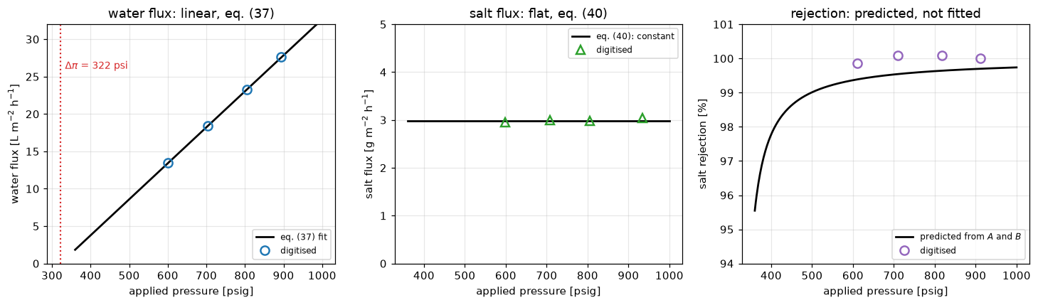
predicted rejection at the four rejection markers: [99.386 99.543 99.642 99.699] %
digitised rejection markers:                       [ 99.85 100.08 100.08 100.  ] %
Validation
Four checks. Two the paper pays for, one on the numerical method, and one on the weakest assumption, which the salt data answer and the water flux alone cannot.
def trend_frac(p, B):
    """Linear trend of B across the pressures p, as a fraction of the mean of B,
    with its standard error (len(p) - 2 degrees of freedom)."""
    slope, icept = np.polyfit(p, B, 1)
    resid = B - (slope * p + icept)
    se = np.sqrt((resid ** 2).sum() / (len(p) - 2) / ((p - p.mean()) ** 2).sum())
    span = np.ptp(p) / B.mean()
    return slope * span, se * span


def b_trend(fit):
    """Trend of the per-point B of a fit across its salt pressures."""
    return trend_frac(fit["p_s"], fit["B_each"])


TREND, TREND_SE = b_trend(FIT)
# a salt flux carried by the water (pore flow) would scale B with the water flux
B_CONV = (FIT["p_s"].max() - FIT["dpi"]) / (FIT["p_s"].min() - FIT["dpi"])
print("1. Eq. 40 is self-checking, and it passes\n"
      f"   B recovered independently from each of the 4 salt points agrees to "
      f"{100*np.ptp(FIT['B_each'])/FIT['B']:.1f} %.\n"
      f"   trend in B across the range: {100*TREND:+.1f} % +/- {100*TREND_SE:.1f} % "
      f"(two degrees of freedom)\n"
      f"   a salt leak carried by the water would make B rise {B_CONV:.2f}-fold over\n"
      f"   the same range, a rise {(B_CONV - 1) / TREND:.0f} times the trend.")
1. Eq. 40 is self-checking, and it passes
B recovered independently from each of the 4 salt points agrees to 2.7 %.
trend in B across the range: +2.4 % +/- 0.8 % (two degrees of freedom)
a salt leak carried by the water would make B rise 2.22-fold over
the same range, a rise 51 times the trend.def film_study(grids=GRIDS, J_lmh=None, delta=50e-6, wall="face"):
"""Relative error of the film wall ratio against its closed form per grid,
and the error ratios between successive grids."""
J_lmh = water.value.max() if J_lmh is None else J_lmh
ex = film_exact(J_lmh, delta)
errs = np.array([abs(film(J_lmh, delta, n=n, wall=wall) - ex) / ex for n in grids])
return errs, errs[:-1] / errs[1:]
ERRS, RATIOS = film_study()
# round-off floor of the finest solve: the same system by a dense LU
_dense = lambda M, b: np.linalg.solve(M.toarray(), b)
SOLVER_GAP = abs(film(water.value.max(), 50e-6, n=GRIDS[-1])
- film(water.value.max(), 50e-6, n=GRIDS[-1], solver=_dense))
NOISE_BOUND = 1e-12
print("2. The film solve reproduces its closed form, and converges\n"
+ "\n".join(f" n = {n:4d} rel err {e:.3e}" for n, e in zip(GRIDS, ERRS))
+ f"\n refinement ratios {np.round(RATIOS, 3)}: first order, as upwind "
"convection must be"
+ f"\n sparse and dense solves at n = {GRIDS[-1]} agree to within {NOISE_BOUND:.0e}"
f" ({SOLVER_GAP <= NOISE_BOUND});\n the finest error is {ERRS[-1]/NOISE_BOUND:.1e} "
"times that bound, so the order is not fitted to round-off")2. The film solve reproduces its closed form, and converges
n = 50 rel err 6.371e-04
n = 100 rel err 3.216e-04
n = 200 rel err 1.616e-04
n = 400 rel err 8.097e-05
n = 800 rel err 4.053e-05
refinement ratios [1.981 1.991 1.995 1.998]: first order, as upwind convection must be
sparse and dense solves at n = 800 agree to within 1e-12 (True);
the finest error is 4.1e+07 times that bound, so the order is not fitted to round-offdef figure_resolution(fit, rej, px_per_pct=PX_PER_PCT, line_px=LINE_PX):
"""What the rejection panel can resolve: the predicted rise across the
measured range and the marker-minus-prediction gaps, in percentage points
and in printed pixels."""
pr = rejection_pct(fit, rej.p_psig.values)
rise = rejection_pct(fit, rej.p_psig.max()) - rejection_pct(fit, rej.p_psig.min())
gap = rej.value.values - pr
return dict(rise=rise, rise_px=rise * px_per_pct, gap_min=gap.min(), gap_max=gap.max(),
gap_px_min=gap.min() * px_per_pct, gap_px_max=gap.max() * px_per_pct,
line_pp=line_px / px_per_pct)
RES = figure_resolution(FIT, rej)
print("3. The rejection prediction, and what the figure can say about it\n"
f" predicted rise across the measured range: {RES['rise']:.3f} percentage points,\n"
f" {RES['rise_px']:.1f} px on the printed figure, whose line is {LINE_PX:.0f} px "
f"({RES['line_pp']:.2f} pp) thick\n"
f" the markers sit {RES['gap_min']:.2f} to {RES['gap_max']:.2f} pp above the "
f"prediction, {RES['gap_px_min']:.0f} to {RES['gap_px_max']:.0f} px:\n"
" about one line width, on circles that straddle the 100 % frame line.\n"
" -> the prediction is consistent with the figure to a line width, and the\n"
" figure has essentially no power to test it.")3. The rejection prediction, and what the figure can say about it
predicted rise across the measured range: 0.313 percentage points,
4.1 px on the printed figure, whose line is 6 px (0.46 pp) thick
the markers sit 0.30 to 0.54 pp above the prediction, 4 to 7 px:
about one line width, on circles that straddle the 100 % frame line.
-> the prediction is consistent with the figure to a line width, and the
figure has essentially no power to test it.Check 4: can concentration polarisation explain the intercept? The fit puts the zero-flux intercept below the caption’s ~350 psi. Polarisation raises the wall osmotic pressure more at high flux than at low, so it bends the flux line concave, and a straight line through a concave curve meets the axis below the true osmotic pressure. To test it, take the caption’s 350 psi as true, put the pymrm film in the loop, \(J = A_\mathrm{true}\,(p - \pi\,c_\mathrm{wall}(J)/c_\mathrm{bulk})\), and ask what a straight-line fit through the four pressures reports.
The true permeability is not known: the membrane is commercial, and the measured \(A\) is itself the apparent slope. So for each film thickness \(A_\mathrm{true}\) is chosen to reproduce the measured slope, and then the intercept is read off. The wall ratio depends on \(J\) and \(\delta\) only through \(J\delta/D\), so the water flux alone fixes only the product of \(A_\mathrm{true}\) and \(\delta\): holding \(A_\mathrm{true}\) at the measured slope and thickening the film gives the same intercept and the same wall ratios. That is why “a film thick enough would lower the apparent permeability” is no test.
The salt flux is the test. The page computes \(B\) from the bulk concentration. If a film raised the wall concentration by \(c_\mathrm{wall}/c_\mathrm{bulk}\), the salt flux would follow the wall, and the \(B\) computed from bulk would rise with pressure in step with the wall ratio. The measured \(B\) is flat to its standard error, so its trend bounds the film.
def apparent_line(delta, A_true, fit, pi=PI_CAPTION, D=D_SALT, wall="face", n=200):
    """Straight line through the polarised fluxes at the water-flux pressures."""
    p_w = fit["p_w"]
    Jv = polarised_fluxes(p_w, A_true, pi,
                          lambda J: film(J, delta, D=D, n=n, wall=wall))
    a, b = np.polyfit(p_w, Jv, 1)
    return dict(A=a, dpi=-b / a, quad=quad_fit(p_w, Jv)[0],
                dev=np.abs(Jv - (a * p_w + b)).max(),
                wall=film(Jv[-1], delta, D=D, n=n, wall=wall))


def matched_A_true(delta, fit, **kw):
    """A_true for which the apparent slope equals the measured one. The slope
    rises with A_true from below the measured value at A_true = A; the upper end
    of the bracket is checked, and brentq raises if it does not bracket."""
    if delta == 0.0:
        return fit["A"]
    return brentq(lambda a: apparent_line(delta, a, fit, **kw)["A"] - fit["A"],
                  fit["A"], 20.0 * fit["A"], xtol=1e-10 * fit["A"], rtol=1e-10)


def polarisation(fit, match_slope=True, deltas_um=(50, 100, 150, 200), **kw):
    """Film thickness at which the apparent intercept equals the fitted one.

    Scans ``deltas_um`` upward for the first sign change of
    (apparent intercept - fitted intercept), then refines it with brentq on
    that bracket. Raises if the scan finds no sign change.
    """
    A_of = (lambda d: matched_A_true(d, fit, **kw)) if match_slope else (lambda d: fit["A"])
    g = lambda d: apparent_line(d, A_of(d), fit, **kw)["dpi"] - fit["dpi"]
    lo = deltas_um[0] * 1e-6
    g_lo = g(lo)
    for d_um in deltas_um[1:]:
        hi = d_um * 1e-6
        g_hi = g(hi)
        if np.sign(g_hi) != np.sign(g_lo):
            break
        lo, g_lo = hi, g_hi
    else:
        raise ValueError("no film thickness in the scan reproduces the fitted intercept")
    d_star = brentq(g, lo, hi, xtol=1e-9)
    a_true = A_of(d_star)
    line = apparent_line(d_star, a_true, fit, **kw)
    return dict(delta=d_star, A_true=a_true, A_ratio=a_true / fit["A"], quad=line["quad"],
                dev=line["dev"], wall=line["wall"])


def salt_trend_under_film(fit, delta, A_true, D=D_SALT, n=200, c_feed=C_FEED):
    """Trend of the B the page would compute from bulk if a film sat on the membrane.

    The fluxes at the salt pressures come from the film in the loop; the salt
    flux follows the wall, J_s = B_true (w c_f - J_s/J_v), with B_true scaled so
    that the mean B computed from bulk equals the fitted one. Returns the trend
    fraction (the statistic measured on the data) and the wall ratios.
    """
    p_s = fit["p_s"]
    wr = lambda J: film(J, delta, D=D, n=n)
    Jv = polarised_fluxes(p_s, A_true, PI_CAPTION, wr)
    w = np.array([wr(J) for J in Jv])
    B_true = fit["B"] / w.mean()
    Js = B_true * w * c_feed / (1.0 + B_true / Jv)
    B_app = Js / (c_feed - Js / (fit["A"] * (p_s - fit["dpi"])))
    return trend_frac(p_s, B_app)[0], w


def salt_limit(fit, trend_max, delta_hi, delta_lo=1e-6, **kw):
    """Thickest film (A_true matched to the slope) whose predicted B trend stays
    at trend_max, and the intercept shift it produces. brentq on
    [delta_lo, delta_hi] raises unless the predicted trend crosses trend_max."""
    g = lambda d: salt_trend_under_film(fit, d, matched_A_true(d, fit, **kw), **kw)[0] - trend_max
    d_max = brentq(g, delta_lo, delta_hi, xtol=1e-9)
    return d_max, PI_CAPTION - apparent_line(d_max, matched_A_true(d_max, fit, **kw), fit, **kw)["dpi"]


rows = [f"{'delta':>9}{'A_true/A':>10}{'apparent dpi':>14}{'curvature':>12}{'c_w/c_b':>9}"]
for d_um in (25, 50, 100):
    a_t = matched_A_true(d_um * 1e-6, FIT)
    ln = apparent_line(d_um * 1e-6, a_t, FIT)
    rows.append(f"{d_um:6.0f} um{a_t/FIT['A']:10.3f}{ln['dpi']:10.0f} psi{ln['quad']:12.2e}"
                f"{ln['wall']:9.3f}")
POL = polarisation(FIT)
K_FILM = D_SALT / POL["delta"]                         # mass-transfer coefficient it implies
SALT_PRED, W_SALT = salt_trend_under_film(FIT, POL["delta"], POL["A_true"])
SALT_T = (SALT_PRED - TREND) / TREND_SE
SALT_P = 2.0 * student_t.sf(abs(SALT_T), df=2)
B_FALL = 1.0 - W_SALT[0] / W_SALT[-1]                  # fall of B_true that would hide the film
TREND_MAX = TREND + 2.0 * TREND_SE
DELTA_MAX, DPI_SHIFT = salt_limit(FIT, TREND_MAX, POL["delta"])
GAP_T = (PI_CAPTION - FIT["dpi"]) / FIT["se_dpi"]
print("4. Can concentration polarisation explain the intercept?\n"
      f"   assumed true osmotic pressure {PI_CAPTION:.0f} psi; A_true matched to the "
      "measured slope\n   " + "\n   ".join(rows) + "\n"
      f"   measured:  A = {FIT['A']:.5f}, dpi = {FIT['dpi']:.0f} psi\n\n"
      f"   water flux alone: a {POL['delta']*1e6:.0f} um film with A_true = "
      f"{POL['A_ratio']:.2f} A reproduces the slope and the intercept,\n"
      f"   wall at {POL['wall']:.2f} times bulk at the highest pressure; it implies "
      f"k = D/delta = {K_FILM:.1e} m/s.\n\n"
      f"   salt flux: that film puts the wall at {np.round(W_SALT, 2)} times bulk at "
      "the four salt pressures,\n"
      f"   so B computed from bulk would rise {100*SALT_PRED:.0f} % across the range; "
      f"measured {100*TREND:+.1f} % +/- {100*TREND_SE:.1f} %:\n"
      f"   {SALT_T:.0f} standard errors, two-sided p = {SALT_P:.4f} with two degrees "
      "of freedom.\n"
      f"   Hiding it would need an intrinsic B that falls {100*B_FALL:.0f} % across "
      "the range in exact step.\n"
      f"   The measured trend plus two standard errors ({100*TREND_MAX:.1f} %) allows a "
      f"film of at most {DELTA_MAX*1e6:.0f} um,\n"
      f"   which lowers the intercept by {DPI_SHIFT:.1f} psi of the "
      f"{PI_CAPTION - FIT['dpi']:.0f} psi gap.\n"
      "   -> the salt data exclude polarisation as the explanation of the gap.\n\n"
      f"   Without polarisation, the gap is {GAP_T:.1f} standard errors of the intercept "
      "(two degrees\n"
      f"   of freedom), and the intercept is an extrapolation "
      f"{FIT['p_w'].min()-FIT['dpi']:.0f} psi beyond the nearest point.")
4. Can concentration polarisation explain the intercept?
assumed true osmotic pressure 350 psi; A_true matched to the measured slope
delta A_true/A apparent dpi curvature c_w/c_b
25 um 1.092 349 psi -4.46e-07 1.128
50 um 1.227 344 psi -1.95e-06 1.275
100 um 1.821 321 psi -9.44e-06 1.657
measured: A = 0.04817, dpi = 322 psi
water flux alone: a 98 um film with A_true = 1.79 A reproduces the slope and the intercept,
wall at 1.64 times bulk at the highest pressure; it implies k = D/delta = 1.5e-05 m/s.
salt flux: that film puts the wall at [1.27 1.4 1.53 1.7 ] times bulk at the four salt pressures,
so B computed from bulk would rise 29 % across the range; measured +2.4 % +/- 0.8 %:
35 standard errors, two-sided p = 0.0008 with two degrees of freedom.
Hiding it would need an intrinsic B that falls 25 % across the range in exact step.
The measured trend plus two standard errors (3.9 %) allows a film of at most 13 um,
which lowers the intercept by 0.3 psi of the 28 psi gap.
-> the salt data exclude polarisation as the explanation of the gap.
Without polarisation, the gap is 3.8 standard errors of the intercept (two degrees
of freedom), and the intercept is an extrapolation 279 psi beyond the nearest point.A weaker, secondary argument: the curvature. The matched film bends the flux line concave, and the four points bend the other way. On the four points’ own scatter the two curvatures differ at a two-sided p of only about 0.09: a quadratic through four points leaves one degree of freedom, so its variance rests on a single residual. With the sidecar’s ordinate error of 1 % instead, the gap is about one to two standard errors, and the film’s departure from a straight line is a few printed pixels, less than the line width this page uses to dismiss the rejection panel. The curvature alone decides nothing.
CURV_GAP = FIT["quad"] - POL["quad"]
CURV_T = CURV_GAP / FIT["se_quad"]
CURV_P = 2.0 * student_t.sf(abs(CURV_T), df=1)
SE_PER_SIGMA = FIT["se_quad"] / FIT["sigma_q"]
J_W = water.value.values
CURV_T_1PCT = CURV_GAP / (SE_PER_SIGMA * 0.01 * np.array([J_W.max(), J_W.min()]))
print("   curvature per psi2: film "
      f"{POL['quad']:+.2e}, data {FIT['quad']:+.2e} +/- {FIT['se_quad']:.1e}\n"
      f"   two-sided p = {CURV_P:.2f} (t = {CURV_T:.1f} on one degree of freedom; the "
      f"residual scatter is {FIT['sigma_q']:.3f} L/(m2 h),\n"
      f"   {FIT['sigma_q']*PX_PER_LMH:.1f} px)\n"
      f"   with a 1 % ordinate error (sidecar) on the largest to the smallest flux: "
      f"{CURV_T_1PCT[0]:.1f} to {CURV_T_1PCT[1]:.1f} standard errors\n"
      f"   the film's flux departs from its own straight line by at most "
      f"{POL['dev']*PX_PER_LMH:.0f} px; the printed line is {LINE_PX:.0f} px")
curvature per psi2: film -9.07e-06, data +7.32e-06 +/- 2.3e-06
two-sided p = 0.09 (t = 7.0 on one degree of freedom; the residual scatter is 0.044 L/(m2 h),
1.9 px)
with a 1 % ordinate error (sidecar) on the largest to the smallest flux: 1.1 to 2.3 standard errors
the film's flux departs from its own straight line by at most 4 px; the printed line is 6 pxClaims
Every number the page states, registered once with how it is checked (docs/claims-design.md). The fitted constants are arithmetic on twelve fixed CSV rows, so they are held tightly; the film errors are discretisation results.
LIN_ERR = 1.0 - (1.0 - np.exp(-X_LIN)) / X_LIN       # Eq. 37 against Eq. 35
WALL_50 = film(water.value.max(), 50e-6)
WALL_100 = film(water.value.max(), 100e-6)
WALL_200 = film(water.value.max(), 200e-6)
ABOVE_100 = 100.0 + 0.5 / PX_PER_PCT                 # half a printed pixel above the frame line

claims.value("A_L_m2_h_psi", FIT["A"], rtol=1e-6, unit="L/(m2 h psi)")
claims.value("delta_pi_psi", FIT["dpi"], rtol=1e-6, unit="psi")
claims.value("delta_pi_se_psi", FIT["se_dpi"], rtol=1e-6, unit="psi")
claims.value("water_flux_r2", FIT["r2"], rtol=1e-9)
claims.value("B_L_m2_h", FIT["B"], rtol=1e-6, unit="L/(m2 h)")
claims.value("B_spread_frac", np.ptp(FIT["B_each"]) / FIT["B"], rtol=1e-6)
claims.value("B_trend_frac", TREND, rtol=1e-6, note="linear trend across the salt pressures")
claims.value("B_trend_se_frac", TREND_SE, rtol=1e-6)
claims.value("B_convective_ratio", B_CONV, rtol=1e-6,
             note="rise of B if the salt flux scaled with the water flux")
claims.value("salt_pressure_ratio", salt.p_psig.max() / salt.p_psig.min(), rtol=1e-9)
claims.value("pressure_spread_first3_max_psi", P_SPREAD[:3].max(), rtol=1e-9)
claims.value("pressure_spread_first3_min_psi", P_SPREAD[:3].min(), rtol=1e-9)
claims.value("pressure_spread_fourth_psi", P_SPREAD[3], rtol=1e-9)
claims.count("rejection_markers_above_100", rej.value.values, ABOVE_100, min_margin=1e-3,
             relative=False, note="readings more than half a printed pixel above 100 %")
claims.value("rejection_predicted_min_pct", R_PRED.min(), rtol=1e-9)
claims.value("rejection_predicted_max_pct", R_PRED.max(), rtol=1e-9)
claims.value("rejection_rise_pp", RES["rise"], rtol=1e-6)
claims.value("rejection_rise_px", RES["rise_px"], rtol=1e-6)
claims.value("axis_over_rise", 100.0 / RES["rise"], rtol=1e-6,
             note="the 0 to 100 % axis against the predicted rise")
claims.value("marker_gap_min_pp", RES["gap_min"], rtol=1e-6)
claims.value("marker_gap_max_pp", RES["gap_max"], rtol=1e-6)
claims.value("marker_gap_min_px", RES["gap_px_min"], rtol=1e-6)
claims.value("marker_gap_max_px", RES["gap_px_max"], rtol=1e-6)
claims.value("line_width_pp", RES["line_pp"], rtol=1e-9)
claims.value("film_err_n400", ERRS[GRIDS.index(400)], rtol=1e-3,
             note="wall ratio on the face against the closed form, 50 um, highest flux")
claims.value("film_err_n800", ERRS[-1], rtol=1e-3)
claims.bound("film_first_order_ratio", RATIOS[-1], min=1.9, max=2.1, basis="theory",
             note="error ratio n = 400 to 800; upwind is first order")
claims.bound("film_two_solver_gap", SOLVER_GAP, max=NOISE_BOUND, basis="tolerance",
             note="sparse against dense LU at n = 800; the round-off floor of the solve")
claims.bound("film_finest_err_over_noise", ERRS[-1] / NOISE_BOUND, min=1e3, basis="chosen",
             note="the finest error must stand 1e3 above the round-off bound for the order to mean anything")
claims.value("film_wall_50um_pct", 100 * (WALL_50 - 1), rtol=1e-4,
             note="at the highest measured water flux")
claims.value("film_wall_100um_pct", 100 * (WALL_100 - 1), rtol=1e-4)
claims.value("film_wall_200um_pct", 100 * (WALL_200 - 1), rtol=1e-4)
claims.value("pol_delta_star_um", POL["delta"] * 1e6, rtol=1e-4)
claims.value("pol_A_true_ratio", POL["A_ratio"], rtol=1e-4)
claims.value("pol_wall_ratio", POL["wall"], rtol=1e-4)
claims.value("pol_k_m_s", K_FILM, rtol=1e-4, unit="m/s")
claims.value("pol_B_trend_pred", SALT_PRED, rtol=1e-4,
             note="B computed from bulk under the matched film")
claims.value("pol_B_trend_gap_se", SALT_T, rtol=1e-4)
claims.value("pol_B_trend_p", SALT_P, rtol=1e-3)
claims.value("pol_B_fall_needed", B_FALL, rtol=1e-4)
claims.value("salt_delta_max_um", DELTA_MAX * 1e6, rtol=1e-4,
             note="predicted B trend equal to the measured trend plus two standard errors")
claims.value("salt_dpi_shift_psi", DPI_SHIFT, rtol=1e-3)
claims.value("pol_curvature", POL["quad"], rtol=1e-3, unit="L/(m2 h psi2)")
claims.value("pol_line_dev_px", POL["dev"] * PX_PER_LMH, rtol=1e-3)
claims.value("data_curvature", FIT["quad"], rtol=1e-6, unit="L/(m2 h psi2)")
claims.value("data_curvature_se", FIT["se_quad"], rtol=1e-6)
claims.value("data_sigma_px", FIT["sigma_q"] * PX_PER_LMH, rtol=1e-6)
claims.value("curvature_gap_p", CURV_P, rtol=1e-3)
claims.value("curvature_gap_se_1pct_min", CURV_T_1PCT[0], rtol=1e-4)
claims.value("curvature_gap_se_1pct_max", CURV_T_1PCT[1], rtol=1e-4)
claims.value("intercept_gap_psi", PI_CAPTION - FIT["dpi"], rtol=1e-6)
claims.value("intercept_gap_se", GAP_T, rtol=1e-6)
claims.value("intercept_extrapolation_psi", FIT["p_w"].min() - FIT["dpi"], rtol=1e-6)
claims.value("eq37_linearisation_err", LIN_ERR, rtol=1e-6,
             note="1 - (1 - exp(-x))/x at the paper's x = 0.06")

# prose numbers, section by section
claims.says("12", "pressure_spread_first3_max_psi")              # The data
claims.says("5", "pressure_spread_first3_min_psi")
claims.says("41", "pressure_spread_fourth_psi")
claims.says("2", "rejection_markers_above_100")
claims.says("2.9 %", "eq37_linearisation_err")                   # Reuse
claims.says("2.7 %", "B_spread_frac")                            # What pymrm adds, meta.yaml
claims.says("1.56", "salt_pressure_ratio")                       # meta.yaml
claims.says("2.4 %", "B_trend_frac")                             # What pymrm adds, meta.yaml
claims.says("0.8 %", "B_trend_se_frac")
claims.says("2.22", "B_convective_ratio")
claims.says("0.31", "rejection_rise_pp")                         # What pymrm adds, meta.yaml
claims.says("4", "rejection_rise_px")
claims.says("320", "axis_over_rise")
claims.says("0.30", "marker_gap_min_pp")
claims.says("0.54", "marker_gap_max_pp")
claims.says("4", "marker_gap_min_px")
claims.says("7", "marker_gap_max_px")
claims.says("0.46", "line_width_pp")
claims.says("29", "film_wall_50um_pct")
claims.says("66", "film_wall_100um_pct")
claims.says("98", "pol_delta_star_um")
claims.says("1.8", "pol_A_true_ratio")
claims.says("1.64", "pol_wall_ratio")
claims.says("1.5e-5", "pol_k_m_s")
claims.says("29 %", "pol_B_trend_pred")
claims.says("35", "pol_B_trend_gap_se")
claims.says("below 0.001", "pol_B_trend_p")
claims.says("25 %", "pol_B_fall_needed")
claims.says("13", "salt_delta_max_um")
claims.says("0.3", "salt_dpi_shift_psi")
claims.says("0.09", "curvature_gap_p")
claims.says("2", "data_sigma_px")
claims.says("4", "pol_line_dev_px")
claims.says("1.1", "curvature_gap_se_1pct_min")
claims.says("2.3", "curvature_gap_se_1pct_max")
claims.says("28", "intercept_gap_psi")
claims.says("3.8", "intercept_gap_se")
claims.says("279", "intercept_extrapolation_psi")
claims.says("0.0482", "A_L_m2_h_psi")                            # meta.yaml agreement
claims.says("322", "delta_pi_psi")
claims.says("7", "delta_pi_se_psi")
claims.says("0.99981", "water_flux_r2")
claims.says("0.0857", "B_L_m2_h")
claims.says("99.39", "rejection_predicted_min_pct")
claims.says("99.70", "rejection_predicted_max_pct")
claims.says("8.1e-5", "film_err_n400")
claims.says("2.00", "film_first_order_ratio")TrueThe defect-injection table
Each row breaks one thing on purpose, re-runs the computation behind a claim with the defect in place, and hands the result to claims.breaks, which records whether the claim’s own check (its tolerance or its bound) catches it. Defects enter where they physically enter: a data row, a parameter, a solver or reading choice. Every claim must be failed by at least one row, and the last cell of the page raises otherwise.
Two pairs in the table are not caught, and both are exact invariances, not blind spots. Shifting every water-flux pressure by the same amount moves the intercept with it and leaves the extrapolation distance unchanged. And the wall ratio depends on \(J\) and \(\delta\) only through \(J\delta/D\), so \((A_\mathrm{true}, \delta) \to (kA_\mathrm{true}, \delta/k)\) scales every flux by \(k\) and leaves the intercept and every wall ratio as they were: holding \(A_\mathrm{true}\) at the measured slope finds a thicker film with the same wall ratio. That invariance is exactly why the water flux alone cannot say whether a film lowered the permeability.
BREAK = []


def brk(name, metric, value):
    """One injected defect: ``value`` is what claim ``metric`` becomes with it."""
    caught = claims.breaks(name, metric, value)
    clean = claims[metric]
    if claims.metrics[metric]["kind"] == "bound":
        clean = "(bound)"     # a bound's own value is not published, and differs between machines
    BREAK.append(dict(defect=name, metric=metric, clean=clean, broken=value, caught=caught))


def fit_claims(fit, rej_frame=rej):
    """The fit and figure claims recomputed from a (broken) fit."""
    res = figure_resolution(fit, rej_frame)
    pr = rejection_pct(fit, rej_frame.p_psig.values)
    tr, tr_se = b_trend(fit)
    return {"A_L_m2_h_psi": fit["A"], "delta_pi_psi": fit["dpi"],
            "delta_pi_se_psi": fit["se_dpi"], "water_flux_r2": fit["r2"],
            "B_L_m2_h": fit["B"], "B_spread_frac": np.ptp(fit["B_each"]) / fit["B"],
            "B_trend_frac": tr, "B_trend_se_frac": tr_se,
            "B_convective_ratio": (fit["p_s"].max() - fit["dpi"]) / (fit["p_s"].min() - fit["dpi"]),
            "rejection_predicted_min_pct": pr.min(), "rejection_predicted_max_pct": pr.max(),
            "rejection_rise_pp": res["rise"], "axis_over_rise": 100.0 / res["rise"],
            "marker_gap_min_pp": res["gap_min"], "marker_gap_max_pp": res["gap_max"],
            "data_curvature": fit["quad"], "data_curvature_se": fit["se_quad"],
            "data_sigma_px": fit["sigma_q"] * PX_PER_LMH,
            "intercept_gap_psi": PI_CAPTION - fit["dpi"],
            "intercept_gap_se": (PI_CAPTION - fit["dpi"]) / fit["se_dpi"],
            "intercept_extrapolation_psi": fit["p_w"].min() - fit["dpi"]}


def pol_claims(fit, **kw):
    """The polarisation claims recomputed from a (broken) fit or film."""
    pol = polarisation(fit, **kw)
    tr, tr_se = b_trend(fit)
    pred, w = salt_trend_under_film(fit, pol["delta"], pol["A_true"], **kw)
    d_max, shift = salt_limit(fit, tr + 2.0 * tr_se, pol["delta"], delta_lo=pol["delta"] / 100, **kw)
    t_salt = (pred - tr) / tr_se
    gap = fit["quad"] - pol["quad"]
    jw = fit["J_w"]
    t1 = gap / (fit["se_quad"] / fit["sigma_q"] * 0.01 * np.array([jw.max(), jw.min()]))
    return {"pol_delta_star_um": pol["delta"] * 1e6, "pol_A_true_ratio": pol["A_ratio"],
            "pol_wall_ratio": pol["wall"], "pol_k_m_s": kw.get("D", D_SALT) / pol["delta"],
            "pol_B_trend_pred": pred, "pol_B_trend_gap_se": t_salt,
            "pol_B_trend_p": 2.0 * student_t.sf(abs(t_salt), df=2),
            "pol_B_fall_needed": 1.0 - w[0] / w[-1],
            "salt_delta_max_um": d_max * 1e6, "salt_dpi_shift_psi": shift,
            "pol_curvature": pol["quad"], "pol_line_dev_px": pol["dev"] * PX_PER_LMH,
            "curvature_gap_p": 2.0 * student_t.sf(abs(gap / fit["se_quad"]), df=1),
            "curvature_gap_se_1pct_min": t1[0], "curvature_gap_se_1pct_max": t1[1]}


def with_value(frame, series_name, p_index, column, new):
    """A copy of the data with one marker of one series changed."""
    out = frame.copy()
    idx = series(out, series_name).index[p_index]
    out.loc[idx, column] = new
    return out


def spread(frame):
    """Spread of the printed pressures per experiment across the three series."""
    return np.ptp(np.vstack([series(frame, s).p_psig.values
                             for s in ("water_flux", "salt_flux", "salt_rejection")]), axis=0)


# --- feed concentration: 3.5 read as g/L --------------------------------------------------------
ROW = "feed 3.5 g/L (the percentage read as g/L)"
_c = fit_claims(fit_membrane(water, salt, c_feed=3.5))
for m in ("B_L_m2_h", "B_spread_frac", "rejection_predicted_min_pct",
          "rejection_predicted_max_pct", "rejection_rise_pp", "axis_over_rise",
          "marker_gap_min_pp", "marker_gap_max_pp"):
    brk(ROW, m, _c[m])

# --- the water-flux pressures: digitisation offset of 12 psi --------------------------------------
ROW = "water-flux pressures read 12 psi high"
_w = water.assign(p_psig=water.p_psig + 12.0)
_c = fit_claims(fit_membrane(_w, salt))
for m in ("delta_pi_psi", "B_convective_ratio", "intercept_gap_psi", "intercept_gap_se",
          "intercept_extrapolation_psi"):
    brk(ROW, m, _c[m])
_sp = spread(obs.assign(p_psig=np.where(obs.series == "water_flux", obs.p_psig + 12.0, obs.p_psig)))
brk(ROW, "pressure_spread_first3_max_psi", _sp[:3].max())
brk(ROW, "pressure_spread_first3_min_psi", _sp[:3].min())

# --- one water-flux marker: the highest read 0.5 L/(m2 h) low ---------------------------------------
ROW = "highest water-flux marker read 0.5 L/(m2 h) low"
_o = with_value(obs, "water_flux", -1, "value", water.value.max() - 0.5)
_fit = fit_membrane(series(_o, "water_flux"), salt)
_c = fit_claims(_fit)
for m in ("A_L_m2_h_psi", "delta_pi_se_psi", "water_flux_r2", "B_trend_se_frac",
          "intercept_extrapolation_psi", "data_curvature", "data_curvature_se", "data_sigma_px"):
    brk(ROW, m, _c[m])
_c = pol_claims(_fit)
for m in ("pol_delta_star_um", "pol_A_true_ratio", "pol_wall_ratio", "pol_k_m_s",
          "pol_B_trend_pred", "pol_B_trend_gap_se", "pol_B_trend_p", "pol_B_fall_needed",
          "salt_delta_max_um", "salt_dpi_shift_psi", "pol_curvature", "pol_line_dev_px",
          "curvature_gap_p", "curvature_gap_se_1pct_min", "curvature_gap_se_1pct_max"):
    brk(ROW, m, _c[m])

# --- the fourth salt triangle placed at the fourth circle's pressure ---------------------------------
ROW = "fourth salt triangle placed at the fourth circle's pressure"
_o = with_value(obs, "salt_flux", -1, "p_psig", water.p_psig.max())
_s = series(_o, "salt_flux")
_fit = fit_membrane(water, _s)
_c = fit_claims(_fit)
for m in ("B_trend_frac", "B_convective_ratio"):
    brk(ROW, m, _c[m])
brk(ROW, "salt_pressure_ratio", _s.p_psig.max() / _s.p_psig.min())
brk(ROW, "pressure_spread_fourth_psi", spread(_o)[3])
_tr, _se = b_trend(_fit)
_d, _shift = salt_limit(_fit, _tr + 2.0 * _se, POL["delta"])
brk(ROW, "salt_delta_max_um", _d * 1e6)
brk(ROW, "salt_dpi_shift_psi", _shift)
_pred = salt_trend_under_film(_fit, POL["delta"], POL["A_true"])[0]
brk(ROW, "pol_B_trend_pred", _pred)
brk(ROW, "pol_B_trend_gap_se", (_pred - _tr) / _se)
brk(ROW, "pol_B_trend_p", 2.0 * student_t.sf(abs((_pred - _tr) / _se), df=2))

# --- the rejection axis calibrated one pixel off ------------------------------------------------------
ROW = "rejection axis calibrated 1 px high"
_rj = rej.assign(value=rej.value - 1.0 / PX_PER_PCT)
_r = figure_resolution(FIT, _rj)
brk(ROW, "rejection_markers_above_100", int(np.sum(_rj.value.values > ABOVE_100)))
brk(ROW, "marker_gap_min_px", _r["gap_px_min"])

# --- the figure read at 300 dpi -----------------------------------------------------------------------
ROW = "pixel scale taken at 300 dpi"
_r = figure_resolution(FIT, rej, px_per_pct=PX_PER_PCT / 2, line_px=LINE_PX)
for key, m in (("rise_px", "rejection_rise_px"), ("gap_px_min", "marker_gap_min_px"),
               ("gap_px_max", "marker_gap_max_px"), ("line_pp", "line_width_pp")):
    brk(ROW, m, _r[key])
brk(ROW, "data_sigma_px", FIT["sigma_q"] * PX_PER_LMH / 2)
brk(ROW, "pol_line_dev_px", POL["dev"] * PX_PER_LMH / 2)

# --- the film: wall value from the last cell centre (pitfall P8) --------------------------------------
ROW = "film wall value read from the last cell centre (P8)"
_e, _ = film_study(wall="cell")
brk(ROW, "film_err_n400", _e[GRIDS.index(400)])
brk(ROW, "film_err_n800", _e[-1])
brk(ROW, "film_wall_50um_pct", 100 * (film(water.value.max(), 50e-6, wall="cell") - 1))

# --- the film: the sign trap of the outward normal -----------------------------------------------------
ROW = "wall condition with the rejection sign flipped (R_int = -0.994)"
for d_um, m in ((50, "film_wall_50um_pct"), (100, "film_wall_100um_pct"),
                (200, "film_wall_200um_pct")):
    brk(ROW, m, 100 * (film(water.value.max(), d_um * 1e-6, R_int=-R_INT) - 1))

# --- the film: diffusivity a decade low ---------------------------------------------------------------
ROW = "salt diffusivity 1.5e-10 m2/s"
_pol = polarisation(FIT, D=D_SALT / 10, deltas_um=(5, 10, 15, 20))
brk(ROW, "pol_delta_star_um", _pol["delta"] * 1e6)
brk(ROW, "salt_delta_max_um",
    1e6 * salt_limit(FIT, TREND_MAX, _pol["delta"], delta_lo=_pol["delta"] / 100,
                     D=D_SALT / 10)[0])
brk(ROW, "film_wall_100um_pct", 100 * (film(water.value.max(), 100e-6, D=D_SALT / 10) - 1))

# --- the polarisation test: A_true held at the measured slope ------------------------------------------
ROW = "A_true held at the measured slope"
_pol = polarisation(FIT, match_slope=False, deltas_um=(50, 100, 150, 200, 250))
brk(ROW, "pol_delta_star_um", _pol["delta"] * 1e6)
brk(ROW, "pol_A_true_ratio", _pol["A_ratio"])
brk(ROW, "pol_wall_ratio", _pol["wall"])
brk(ROW, "pol_curvature", _pol["quad"])

# --- the refinement study ----------------------------------------------------------------------------
_, _r = film_study(grids=(50, 100, 200, 400, 600))
brk("finest grid 600 cells, read as a doubling", "film_first_order_ratio", _r[-1])
brk("second solve on 799 cells", "film_two_solver_gap",
    abs(film(water.value.max(), 50e-6, n=GRIDS[-1] - 1) - film(water.value.max(), 50e-6,
                                                                n=GRIDS[-1])))
brk("reference taken from the n = 800 solve", "film_finest_err_over_noise",
    abs(film(water.value.max(), 50e-6, n=GRIDS[-1]) - film(water.value.max(), 50e-6,
                                                            n=GRIDS[-1])) / NOISE_BOUND)

# --- Eq. 37: the linearisation at a larger argument ------------------------------------------------------
_x = 0.08
brk("Eq. 37 linearised at x = 0.08", "eq37_linearisation_err",
    1.0 - (1.0 - np.exp(-_x)) / _x)

pd.set_option("display.width", 200)
print(pd.DataFrame(BREAK).to_string(index=False, formatters={
    "clean": lambda v: f"{v:.5g}" if isinstance(v, float) else str(v),
    "broken": lambda v: f"{v:.5g}" if isinstance(v, float) else str(v)}))
defect metric clean broken caught
feed 3.5 g/L (the percentage read as g/L) B_L_m2_h 0.085746 0.89283 True
feed 3.5 g/L (the percentage read as g/L) B_spread_frac 0.026951 0.016193 True
feed 3.5 g/L (the percentage read as g/L) rejection_predicted_min_pct 99.386 93.953 True
feed 3.5 g/L (the percentage read as g/L) rejection_predicted_max_pct 99.699 96.953 True
feed 3.5 g/L (the percentage read as g/L) rejection_rise_pp 0.31338 2.9998 True
feed 3.5 g/L (the percentage read as g/L) axis_over_rise 319.1 33.336 True
feed 3.5 g/L (the percentage read as g/L) marker_gap_min_pp 0.30089 3.0468 True
feed 3.5 g/L (the percentage read as g/L) marker_gap_max_pp 0.53691 5.8965 True
water-flux pressures read 12 psi high delta_pi_psi 321.8 333.8 True
water-flux pressures read 12 psi high B_convective_ratio 2.2197 2.2751 True
water-flux pressures read 12 psi high intercept_gap_psi 28.195 16.195 True
water-flux pressures read 12 psi high intercept_gap_se 3.8348 2.1688 True
water-flux pressures read 12 psi high intercept_extrapolation_psi 279 279 False
water-flux pressures read 12 psi high pressure_spread_first3_max_psi 12.1 15.1 True
water-flux pressures read 12 psi high pressure_spread_first3_min_psi 5.2 7.5 True
highest water-flux marker read 0.5 L/(m2 h) low A_L_m2_h_psi 0.048172 0.04669 True
highest water-flux marker read 0.5 L/(m2 h) low delta_pi_se_psi 7.3524 7.633 True
highest water-flux marker read 0.5 L/(m2 h) low water_flux_r2 0.99981 0.9998 True
highest water-flux marker read 0.5 L/(m2 h) low B_trend_se_frac 0.0076086 0.0076072 True
highest water-flux marker read 0.5 L/(m2 h) low intercept_extrapolation_psi 279 289.94 True
highest water-flux marker read 0.5 L/(m2 h) low data_curvature 7.3218e-06 -6.2126e-06 True
highest water-flux marker read 0.5 L/(m2 h) low data_curvature_se 2.3249e-06 4.5995e-06 True
highest water-flux marker read 0.5 L/(m2 h) low data_sigma_px 1.9089 3.7764 True
highest water-flux marker read 0.5 L/(m2 h) low pol_delta_star_um 98.352 114.26 True
highest water-flux marker read 0.5 L/(m2 h) low pol_A_true_ratio 1.7863 2.1026 True
highest water-flux marker read 0.5 L/(m2 h) low pol_wall_ratio 1.6415 1.7645 True
highest water-flux marker read 0.5 L/(m2 h) low pol_k_m_s 1.5251e-05 1.3128e-05 True
highest water-flux marker read 0.5 L/(m2 h) low pol_B_trend_pred 0.29016 0.32538 True
highest water-flux marker read 0.5 L/(m2 h) low pol_B_trend_gap_se 34.978 39.603 True
highest water-flux marker read 0.5 L/(m2 h) low pol_B_trend_p 0.00081636 0.00063698 True
highest water-flux marker read 0.5 L/(m2 h) low pol_B_fall_needed 0.25172 0.27786 True
highest water-flux marker read 0.5 L/(m2 h) low salt_delta_max_um 12.967 13.335 True
highest water-flux marker read 0.5 L/(m2 h) low salt_dpi_shift_psi 0.34299 0.34074 True
highest water-flux marker read 0.5 L/(m2 h) low pol_curvature -9.0656e-06 -1.1765e-05 True
highest water-flux marker read 0.5 L/(m2 h) low pol_line_dev_px 4.0895 5.3457 True
highest water-flux marker read 0.5 L/(m2 h) low curvature_gap_p 0.08972 0.44043 True
highest water-flux marker read 0.5 L/(m2 h) low curvature_gap_se_1pct_min 1.1171 0.38544 True
highest water-flux marker read 0.5 L/(m2 h) low curvature_gap_se_1pct_max 2.2863 0.77459 True
fourth salt triangle placed at the fourth circle's pressure B_trend_frac 0.024025 0.023225 True
fourth salt triangle placed at the fourth circle's pressure B_convective_ratio 2.2197 2.0725 True
fourth salt triangle placed at the fourth circle's pressure salt_pressure_ratio 1.563 1.4951 True
fourth salt triangle placed at the fourth circle's pressure pressure_spread_fourth_psi 40.6 18 True
fourth salt triangle placed at the fourth circle's pressure salt_delta_max_um 12.967 15.239 True
fourth salt triangle placed at the fourth circle's pressure salt_dpi_shift_psi 0.34299 0.4766 True
fourth salt triangle placed at the fourth circle's pressure pol_B_trend_pred 0.29016 0.25485 True
fourth salt triangle placed at the fourth circle's pressure pol_B_trend_gap_se 34.978 26.878 True
fourth salt triangle placed at the fourth circle's pressure pol_B_trend_p 0.00081636 0.0013813 True
rejection axis calibrated 1 px high rejection_markers_above_100 2 0 True
rejection axis calibrated 1 px high marker_gap_min_px 3.9417 2.9417 True
pixel scale taken at 300 dpi rejection_rise_px 4.1053 2.0526 True
pixel scale taken at 300 dpi marker_gap_min_px 3.9417 1.9708 True
pixel scale taken at 300 dpi marker_gap_max_px 7.0335 3.5168 True
pixel scale taken at 300 dpi line_width_pp 0.45802 0.91603 True
pixel scale taken at 300 dpi data_sigma_px 1.9089 0.95445 True
pixel scale taken at 300 dpi pol_line_dev_px 4.0895 2.0447 True
film wall value read from the last cell centre (P8) film_err_n400 8.0967e-05 0.00039869 True
film wall value read from the last cell centre (P8) film_err_n800 4.0531e-05 0.00019942 True
film wall value read from the last cell centre (P8) film_wall_50um_pct 28.913 28.872 True
wall condition with the rejection sign flipped (R_int = -0.994) film_wall_50um_pct 28.913 -18.32 True
wall condition with the rejection sign flipped (R_int = -0.994) film_wall_100um_pct 66.075 -28.462 True
wall condition with the rejection sign flipped (R_int = -0.994) film_wall_200um_pct 174.91 -38.884 True
salt diffusivity 1.5e-10 m2/s pol_delta_star_um 98.352 9.8352 True
salt diffusivity 1.5e-10 m2/s salt_delta_max_um 12.967 1.2967 True
salt diffusivity 1.5e-10 m2/s film_wall_100um_pct 66.075 8123.2 True
A_true held at the measured slope pol_delta_star_um 98.352 175.69 True
A_true held at the measured slope pol_A_true_ratio 1.7863 1 True
A_true held at the measured slope pol_wall_ratio 1.6415 1.6415 False
A_true held at the measured slope pol_curvature -9.0656e-06 -5.0749e-06 True
finest grid 600 cells, read as a doubling film_first_order_ratio (bound) 1.4988 True
second solve on 799 cells film_two_solver_gap (bound) 6.5331e-08 True
reference taken from the n = 800 solve film_finest_err_over_noise (bound) 0 True
Eq. 37 linearised at x = 0.08 eq37_linearisation_err 0.029409 0.038954 TrueWhat pymrm adds
The honest headline is a negative one, and it is the most useful thing here.
The third panel of Figure 5 looks like a validation of the solution-diffusion model: rejection climbs with pressure and flattens near 100 %, exactly as the theory says. Closing the model shows that panel predicts a rise of 0.31 percentage points across the measured range, about 4 pixels on a printed figure whose line is 6 pixels (0.46 percentage points) thick. The markers sit 0.30 to 0.54 percentage points above the prediction, 4 to 7 pixels, about one line width, on circles that straddle the 100 % frame line. On this axis a prediction anywhere within a line width of the markers looks the same. The agreement in that panel is not evidence. The real content of Figure 5 is in the first two panels, where the linear water flux and the flat salt flux are each resolved over their full range: \(B\) recovered point by point agrees to 2.7 %, with a trend of 2.4 % (standard error 0.8 %, two degrees of freedom) across the range, where a salt leak carried by the water would make it rise 2.22-fold.
That is worth stating plainly because it generalises: a quantity plotted on an axis that spans 320 times the effect being tested cannot test it, however good the agreement looks.
Second, a test of the weakest assumption. The derivation, as this page transcribes it, assumes no polarisation; the page quotes nothing from the source on whether it was examined. The pymrm film solve puts numbers on it: at the highest measured flux a 50 µm boundary layer raises the wall concentration 29 % above bulk, and a 100 µm one 66 %. On the water flux alone, the film could explain the 28 psi gap between the fitted intercept and the caption’s osmotic pressure: a 98 µm film, with a true permeability 1.8 times the apparent one, reproduces both the measured slope and the intercept, with the wall at 1.64 times bulk at the highest pressure. That film implies a mass-transfer coefficient of 1.5e-5 m/s, plausible only in a poorly mixed cell, and the page has no apparatus details to say which.
The salt data exclude it. The page’s \(B\) is computed from the bulk concentration; under that film the salt flux would follow the wall, and \(B\) would rise 29 % across the range. The measured trend is 2.4 %, 35 standard errors below, two-sided p below 0.001 with two degrees of freedom. Hiding the film would need an intrinsic \(B\) that falls by 25 % across the range in exact step with the wall. The measured trend plus two standard errors allows a film of at most 13 µm, which moves the intercept by 0.3 psi. So polarisation does not explain the gap. The curvature of the water flux points the same way, but weakly: two-sided p = 0.09 on one degree of freedom, a residual scatter of 2 px, a film departing from a straight line by 4 px against a 6 px printed line, and only 1.1 to 2.3 standard errors with the sidecar’s 1 % ordinate error.
J_MAX = water.value.max()
x50, c50 = film(J_MAX, 50e-6, profile=True)
x100, c100 = film(J_MAX, 100e-6, profile=True)
fig, ax = plt.subplots(1, 2, figsize=(11.6, 4.0))
ax[0].plot(x50 * 1e6, c50, lw=2, color="tab:blue", label="50 $\\mu$m film")
ax[0].plot(x100 * 1e6, c100, lw=2, color="tab:red", label="100 $\\mu$m film")
ax[0].axhline(1.0, color="k", lw=1)
ax[0].set(xlabel="distance from bulk [$\\mu$m]", ylabel="$c/c_\\mathrm{bulk}$",
          title="salt piles up against the membrane\n(at the highest measured flux)")
ax[0].legend(fontsize=8)

JL = np.linspace(2, 40, 60)
for dl, col in ((25e-6, "tab:green"), (50e-6, "tab:blue"), (100e-6, "tab:orange"),
                (200e-6, "tab:red")):
    ax[1].plot(JL, [film(j, dl) for j in JL], lw=1.8, color=col, label=f"{dl*1e6:.0f} $\\mu$m")
ax[1].axvspan(water.value.min(), J_MAX, color="grey", alpha=0.18)
ax[1].text(water.value.mean(), 1.02, "measured", ha="center", fontsize=8, color="0.35")
ax[1].set(xlabel="water flux [L m$^{-2}$ h$^{-1}$]",
          ylabel="$c_\\mathrm{wall}/c_\\mathrm{bulk}$",
          title="how much polarisation, for a film you cannot see")
ax[1].legend(fontsize=8, title="film", title_fontsize=8)
fig.tight_layout(); plt.show()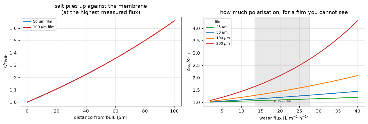
What this page does not establish. It rests on a single figure of a review article, four points per series, and the membrane is a commercial one whose \(A\) and \(B\) are not independently known, so the fitted constants cannot be checked against anything. The film thickness is a free parameter: the polarisation numbers above are a sensitivity study, not a measurement. The intercept sits 28 psi below the caption’s stated osmotic pressure, 3.8 standard errors of the fit with two degrees of freedom, and it is an extrapolation 279 psi beyond the nearest point; a systematic offset of the pressure axis moves it one for one. Polarisation does not explain it: the salt data limit the film to a shift of a fraction of a psi, unless the intrinsic \(B\) falls with pressure in exact step with the wall, which nothing here can exclude. Nothing on this page explains the gap. The caption’s “~350 psi” is a round number, not a measurement on this feed. The intrinsic rejection used in the film solve is taken as 0.994 from the model itself, which makes that part mildly circular; the wall ratio depends on it only through the small permeating fraction.
Reuse
The film solve is the reusable piece. film_wall_ratio in model.py takes SI arguments and knows nothing about this membrane: give it a permeate velocity, a film thickness, a diffusivity and an intrinsic rejection, and it returns the wall enrichment, read on the membrane face. It is the concentration-polarisation closure any pressure-driven membrane model needs, and it is a plain S3 convection-diffusion solve, so it extends directly: variable diffusivity, a reacting boundary layer, or a second solute all drop into the same assembly. polarised_fluxes puts it in the loop of the flux equation, with a bracket that is proved, not guessed.
To adapt to your system: change C_FEED and the osmotic pressure, refit A and B to your own flux data, and set D_SALT for your solute. Nothing else on the page is specific to seawater.
The one trap. The wall boundary condition uses the outward normal, which at the downstream face points in \(+x\); the rejected-salt term therefore enters with a minus sign. Getting that sign wrong gives a wall concentration below bulk, salt depleting against the membrane it cannot cross, which is physically impossible and a useful thing to check for (a row of the defect table).
Range of validity. Eq. 37 is a linearisation of Eq. 35 valid while \(v_i(\Delta p-\Delta\pi)/RT \ll 1\); the paper notes this is about 0.06 for reverse osmosis, so the error is 2.9 %. At pervaporation conditions, where the permeate pressure approaches vacuum, the exponential must be kept.
Related pages. H1.8, H1.13 (other membrane transport), A2.3 (the same S3 machinery for dispersion), F3.1 (film transport with reaction).
Cite the source, not this page: Wijmans, J. G. and Baker, R. W., The solution-diffusion model: a review, Journal of Membrane Science 107(1-2) 1-21 (1995), doi:10.1016/0376-7388(95)00102-I.
# Claims: prints every registered number, writes agreement.json for CI, and
# raises when a claim fails its own check or has no break row.
claims.report();   # the semicolon keeps the notebook from echoing the payload
Claims for H1.7:
A_L_m2_h_psi = 0.048172 value rtol 1e-06
delta_pi_psi = 321.8 value rtol 1e-06
delta_pi_se_psi = 7.3524 value rtol 1e-06
water_flux_r2 = 0.99981 value rtol 1e-09
B_L_m2_h = 0.085746 value rtol 1e-06
B_spread_frac = 0.026951 value rtol 1e-06
B_trend_frac = 0.024025 value rtol 1e-06
B_trend_se_frac = 0.0076086 value rtol 1e-06
B_convective_ratio = 2.2197 value rtol 1e-06
salt_pressure_ratio = 1.563 value rtol 1e-09
pressure_spread_first3_max_psi = 12.1 value rtol 1e-09
pressure_spread_first3_min_psi = 5.2 value rtol 1e-09
pressure_spread_fourth_psi = 40.6 value rtol 1e-09
rejection_markers_above_100 = 2 exact exact, margin 0.0382
rejection_predicted_min_pct = 99.386 value rtol 1e-09
rejection_predicted_max_pct = 99.699 value rtol 1e-09
rejection_rise_pp = 0.31338 value rtol 1e-06
rejection_rise_px = 4.1053 value rtol 1e-06
axis_over_rise = 319.1 value rtol 1e-06
marker_gap_min_pp = 0.30089 value rtol 1e-06
marker_gap_max_pp = 0.53691 value rtol 1e-06
marker_gap_min_px = 3.9417 value rtol 1e-06
marker_gap_max_px = 7.0335 value rtol 1e-06
line_width_pp = 0.45802 value rtol 1e-09
film_err_n400 = 8.0967e-05 value rtol 0.001
film_err_n800 = 4.0531e-05 value rtol 0.001
film_first_order_ratio = (here 2.0e+00) bound bound [1.9, 2.1] [theory]
film_two_solver_gap = (here 2.2e-16) bound bound <= 1e-12 [tolerance]
film_finest_err_over_noise = (here 4.1e+07) bound bound >= 1000 [chosen]
film_wall_50um_pct = 28.913 value rtol 0.0001
film_wall_100um_pct = 66.075 value rtol 0.0001
film_wall_200um_pct = 174.91 value rtol 0.0001
pol_delta_star_um = 98.352 value rtol 0.0001
pol_A_true_ratio = 1.7863 value rtol 0.0001
pol_wall_ratio = 1.6415 value rtol 0.0001
pol_k_m_s = 1.5251e-05 value rtol 0.0001
pol_B_trend_pred = 0.29016 value rtol 0.0001
pol_B_trend_gap_se = 34.978 value rtol 0.0001
pol_B_trend_p = 0.00081636 value rtol 0.001
pol_B_fall_needed = 0.25172 value rtol 0.0001
salt_delta_max_um = 12.967 value rtol 0.0001
salt_dpi_shift_psi = 0.34299 value rtol 0.001
pol_curvature = -9.0656e-06 value rtol 0.001
pol_line_dev_px = 4.0895 value rtol 0.001
data_curvature = 7.3218e-06 value rtol 1e-06
data_curvature_se = 2.3249e-06 value rtol 1e-06
data_sigma_px = 1.9089 value rtol 1e-06
curvature_gap_p = 0.08972 value rtol 0.001
curvature_gap_se_1pct_min = 1.1171 value rtol 0.0001
curvature_gap_se_1pct_max = 2.2863 value rtol 0.0001
intercept_gap_psi = 28.195 value rtol 1e-06
intercept_gap_se = 3.8348 value rtol 1e-06
intercept_extrapolation_psi = 279 value rtol 1e-06
eq37_linearisation_err = 0.029409 value rtol 1e-06