The two-phase theory, tested against the measurements it was born with

Toomey and Johnstone wrote the two-phase postulate down as an equality in 1952 and then, four columns later, printed intercepts that refute half of it. The intercepts are read off Lewis, Gilliland and Bauer’s particles, not their own, and the paper says so; this page separates the half those numbers support from the half they do not, and shows why the authors’ own beads cannot settle it.

The two-phase theory, tested against the measurements it was born with

Catalog ID: E1.1 · Structures: S7 · Tier: T0

Every bubbling-bed model in the literature starts from one line:

\[(u_f - u_{mf})\,A \;=\; V_g \qquad \text{(their equation 3)}\]

all the gas beyond what minimum fluidisation needs leaves as bubbles, so the dense phase sees the same flow however hard the bed is blown. Kunii and Levenspiel’s \(\delta = (u_0-u_{mf})/u_b\), reproduced on the published E2.1 page, is that line divided by a bubble velocity, and E2.1 assumes it: nothing on that page is compared with a measurement, and it says so.

This page is the other half of the pair. Toomey and Johnstone printed the postulate and numbers that test it.

Whose particles the headline is about, read this first. The four intercept ratios this page turns on are printed by Toomey and Johnstone, but they are read off Lewis, Gilliland and Bauer’s four particle sizes, not off the five bead sizes tabulated in this paper. The authors say so in the sentence before them: only Lewis, Gilliland and Bauer’s data “extend to low enough velocities to obtain an accurate indication of the point of intersection”. Their Figure 3 labels seven curves and separates them in its own legend, three filled, “AUTHORS’ DATA”, at \(D_p = 0.0148''\), \(0.00861''\) and \(0.00418''\), and four open, “DATA OF LEWIS, GILLILAND AND BAUER”, at \(0.0224''\), \(0.0178''\), \(0.0112''\) and \(0.00881''\). Four open curves, four printed ratios.

So this page is a statement about the postulate, tested on numbers Toomey and Johnstone printed and read; it is not a statement about this apparatus. Section 4 runs the refit on the authors’ own beads anyway, the one this page declines to rely on, and shows that those beads cannot fix even the sign of the effect, which is what makes Lewis, Gilliland and Bauer’s ratios load-bearing rather than incidental.

With that said, the postulate has two testable halves and the printed numbers separate them:

• the half they support, the dense-phase flow really is constant, independent of \(u_f\);
• the half they refute, that constant is not \(u_{mf}\). The printed intercept ratios \(u_{mf}/u_e =\) 0.85, 0.69, 0.83, 0.87 put the dense phase 15 to 45 % above minimum fluidisation, so the visible bubble flow falls short of \((u_f-u_{mf})A\) by exactly that much.

Everything after 1952 kept the second half. This page also finds a third problem the authors flag and never compute: their beds drop a tenth of an atmosphere, so \(u_f\) itself is not a single number, the quantity in equation 3 varies by about a quarter across the bed at the velocities where the intercept is taken (a fifth if the air is at room temperature rather than the 200 °F the paper states; both figures are computed). That part is a pymrm solve.

# Bootstrap: the pymrm this page was checked with, and the gallery files it was
# published with. Works in a checkout, in CI and on a fresh Colab VM.
GALLERY_REF = "gallery-2026.11.10.3"  # replaced by the release tag at publication
PYMRM = ">=3.3.0,<4"  # equals meta.yaml pymrm_min_version, up to the next major
PAGE = "E1.1-two-phase-theory"  # equals the page directory

import os, sys, urllib.request
from pathlib import Path
_shared = next((p / "shared" for p in (Path.cwd(), *Path.cwd().parents)
                if (p / "shared" / "gallery_bootstrap.py").is_file()), None)
if _shared is None:
    _shared = (Path(os.environ.get("XDG_CACHE_HOME") or Path.home() / ".cache")
               / "pymrm-gallery" / GALLERY_REF)
    _shared.mkdir(parents=True, exist_ok=True)
    urllib.request.urlretrieve(
        "https://raw.githubusercontent.com/computational-chemical-engineering/"
        f"pymrm-gallery/{GALLERY_REF}/shared/gallery_bootstrap.py",
        _shared / "gallery_bootstrap.py")
sys.path.insert(0, str(_shared))
sys.modules.pop("gallery_bootstrap", None)
from gallery_bootstrap import setup
setup(PAGE, PYMRM, GALLERY_REF);  # the semicolon stops the cell echoing the path

# Imports. The page's model.py is put on sys.path by setup().
import numpy as np
import pandas as pd
import matplotlib.pyplot as plt
from pymrm.checks import find_roots, observed_orders
from gallery_utils import Claims, cite_data, load_claims, load_data, load_meta
from model import PATM, CompressibleBed, mu_air, rho_air

plt.rcParams.update({"figure.dpi": 120, "font.size": 9, "axes.grid": True,
                     "grid.alpha": 0.3, "figure.autolayout": True})
claims = Claims(PAGE.split("-")[0])
BREAK = []   # (injected defect, claim, clean value, broken value, caught)


def brk(row, metric, broken):
    """One injected defect: ``broken`` is what claim ``metric`` becomes with it.

    ``broken`` may be a zero-argument callable; a solve that fails under the
    defect is recorded as nan (caught) with the reason in the row label."""
    if callable(broken):
        try:
            broken = broken()
        except Exception as exc:                       # noqa: BLE001
            row, broken = f"{row} [solve fails: {type(exc).__name__}]", np.nan
    caught = claims.breaks(row, metric, broken)
    BREAK.append((row, metric, claims[metric], broken, caught))
    return caught

Background

A fluidised bed blown harder than \(u_{mf}\) does not stay uniform. It splits into a dense, particle-rich continuous phase and gas voids, Toomey and Johnstone’s discontinuous phase, everyone else’s bubbles. The question the whole subject turns on is how the gas divides between them.

The two-phase theory answers it with an accounting identity: the continuous phase keeps exactly the flow it needed to be fluidised at all, \(u_{mf}\), and every cubic foot per second above that goes into bubbles. It is attractive because it needs nothing measured, no bubble size, no exchange coefficient, no interstitial velocity. It is the reason a bubbling-bed reactor model can be written on one page.

It is also, in the strong form, wrong, and it has been known to be wrong since the 1970s; the modern statement puts a visible bubble flow factor \(Y<1\) in front of it. What is less well known is that the paper the postulate is attributed to already contains the measurement that breaks it, in its own text, four columns after the equation.

How this page is sourced. Toomey and Johnstone (1952) predates DOIs; there is no DOI for it and none was invented. The reprint route was tried and failed, Kunii and Levenspiel (1968) state the relation as their equations 2 and 3 but never name it “two-phase theory”, never attribute it to Toomey and Johnstone (their whole Literature Cited list was read), and never test it; Froment, De Wilde and Bischoff’s third edition does not contain the string “Toomey” at all. So this page is built from the original, read off 400 dpi renders. The PDF has no text layer whatsoever, pdftotext returns one byte per page, so every digit here came off a picture of the printed page and every questionable one is flagged in the dataset sidecars.

The published model

The paper’s argument runs in three moves. All three are on journal page 223.

1. An empirical expansion law, borrowed. Lewis, Gilliland and Bauer’s correlation for how far a bed swells above its incipient height:

\[1 - \frac{L_{mf}}{L_f} \;=\; \frac{0.065}{D_p^{0.5}}\,(u_f - u_{mf}) \qquad (1)\]

with \(D_p\) in feet and velocities in ft/s, so the constant 0.065 carries \(\mathrm{s\,ft^{-1/2}}\). The left-hand side is the fraction of the expanded bed that is void space added by fluidisation, the bubble fraction \(\delta\).

2. The postulate. Rewriting (1) with \(V_b\), the volume of discontinuous phase held in the bed at any instant,

\[\frac{V_b}{A L_f} = \frac{0.065}{D_p^{0.5}}(u_f - u_{mf}) \qquad (2)\]

and then asserting

\[(u_f - u_{mf})\,A = V_g \qquad (3)\]

where \(V_g\) is the volume of discontinuous phase flowing per unit time. (3) is the two-phase theory. It is stated as an equality, with no error bar and no supporting measurement beside it.

3. What (1) and (3) together imply. Dividing,

\[t_d \;=\; \frac{V_b}{V_g} \;=\; \frac{0.065\,L_f}{D_p^{0.5}} \qquad (4)\]

so the residence time of a bubble depends only on bed height and particle size, and the bubble velocity \(L_f/t_d = D_p^{0.5}/0.065\) depends on nothing but the particle diameter, not on gas velocity, not on bubble size.

The rest of the paper is a separate energy argument that ends in

\[\Delta P_{ke} = (K D_p^{0.5} - k)(\rho_m-\rho_g) L_f \ln\frac{V}{V_e} \qquad (10)\]

\[\ln\frac{V}{V_e} = \frac{1}{(K D_p^{0.5}-k)}\,\frac{\Delta P_{ke}}{\Delta P_{mf}} \qquad (11)\]

for the pressure drop in excess of the bed weight, \(\Delta P_{ke}\), which they attribute to kinetic-energy loss in particle collisions. Equation (11) is what makes this page possible: \(V_e\) is the gas flow at which the discontinuous phase first appears, and it is obtained as the intercept of straight lines fitted to measured \(\Delta P_{ke}/\Delta P_{mf}\) against \(\ln G\). If (3) is right, that intercept must land exactly on \(u_{mf}\).

The authors report where it actually lands, for Lewis, Gilliland and Bauer’s particles, which is what the preceding sentence restricts it to:

“Only the data of Lewis, Gilliland and Bauer (12) extend to low enough velocities to obtain an accurate indication of the point of intersection. … For the four particle diameters, the ratio \(u_{mf}/u_e\) is 0.85, 0.69, 0.83, 0.87.”

and then read it as a confirmation:

“Thus, only a slight increase in gas velocity over that at incipient fluidization is needed to reach the critical condition where the discontinuous phase forms.”

It is a slight increase. It is also, as this page measures, the whole difference between the two-phase theory and the data.

Parameters and assumptions

Everything the page needs is either printed by the paper or is a unit conversion. Four things are assumptions and are named here so they can be argued with:

1. Air temperature 200 °F. The paper states that the fluidising medium was “filtered air, delivered to the system at about 200 °F. and one per cent relative humidity”. Gas viscosity enters only through the conversion from the printed mass velocities \(G\) to velocity ratios \(u_f/u_{mf}\), and that ratio turns out to depend on \(\mu\) alone (below). Every velocity ratio on this page is therefore given with its 70 °F counterpart as a sensitivity.
2. The five printed Reynolds numbers belong to bead sizes 5, 4, 3, 2, 1. The paper prints them as a bare ascending list with no labels. Ascending \(Re\) with ascending \(D_p\) is the only sensible reading, and the bead numbering runs largest-first. This is recorded as an inference in the dataset.
3. The bed exhausts to atmosphere, \(P_{top} = 101\,325\) Pa. The gas leaves through a cyclone (p. 220), so this is the natural datum; the page reports how much the pymrm results move if it is 10 % higher, and a break row raises it tenfold.
4. Minimum-fluidisation velocity is pressure-independent. In the viscous regime \(u_{mf}\) depends on \(\mu\) and not on \(\rho_g\), and the paper’s own \(Re_{mf}\) run from 0.014 to 12.2, so all but the coarsest bead is deeply viscous. Assumed constant with height in the compressible solve.

The conversions: 1 in. = 0.0254 m; 1 in. H₂O = \(1000 \times 9.80665 \times 0.0254\) Pa = 249.089 Pa (= 5.2023 lbf/ft², the classical engineering value); 1 lb/ft³ = 16.0185 kg/m³; 1 lb/(hr)(ft²) = \(1.35623\times10^{-3}\) kg/(m² s).

# ---- unit conversions, all printed so nothing is retyped (mu_air, rho_air in model.py)
IN, FT       = 0.0254, 0.3048
INH2O        = 1000.0 * 9.80665 * 0.0254          # Pa per inch of water
LBF_FT2      = 47.880259                          # Pa per lbf/ft2
LB_FT3       = 16.0185                            # kg/m3 per lb/ft3
G_SI         = 0.45359237 / (3600 * 0.09290304)   # kg/(m2 s) per lb/(hr ft2)
G_ACC        = 9.80665                            # m/s2

T_PAPER, T_ROOM = 366.483, 294.261   # 200 F and 70 F
print(f"1 in.H2O = {INH2O:.3f} Pa = {INH2O / LBF_FT2:.4f} lbf/ft^2")
print(f"1 lb/(hr ft2) = {G_SI:.5e} kg/(m2 s);  P_top = {PATM:.0f} Pa")
print(f"mu_air(200 F) = {mu_air(T_PAPER):.4e} Pa s   rho_air(200 F) = {rho_air(T_PAPER):.5f} kg/m3")
print(f"mu_air( 70 F) = {mu_air(T_ROOM):.4e} Pa s   rho_air( 70 F) = {rho_air(T_ROOM):.5f} kg/m3")

1 in.H2O = 249.089 Pa = 5.2023 lbf/ft^2
1 lb/(hr ft2) = 1.35623e-03 kg/(m2 s);  P_top = 101325 Pa
mu_air(200 F) = 2.1449e-05 Pa s   rho_air(200 F) = 0.96316 kg/m3
mu_air( 70 F) = 1.8186e-05 Pa s   rho_air( 70 F) = 1.19955 kg/m3

The data

Four files, all transcribed from 400 dpi renders of a scan with no text layer at all.

file	what it is
..._table1_beads.csv	Table 1, the five Scotchlite glass bead sizes, 5 rows
..._table2_pressure_losses.csv	Table 2, 41 runs: mass velocity, \(\Delta P_{mf}\), \(L_{mf}\), \(\Delta P_{ke}/\Delta P_{mf}\)
..._table3_wall_velocities.csv	Table 3, 13 runs of particle velocity at the wall from 16-mm Fastax film, and \(\Delta P_{ke}/L\)
..._printed_results.csv	the scalars printed in the running text: the five \(Re_{mf}\), the four \(u_{mf}/u_e\), the 0.065 of eq. (1), the column geometry

This page loads no other page’s dataset, so the cross-page reading rule does not bite. It does cite E2.1’s findings in prose (the split reproduced there against Kunii and Levenspiel’s Appendix C, read from its claims below, and that page’s own statement that nothing on it is compared with a measurement), and E1.2 for single-bubble hydrodynamics, which this page deliberately stays out of.

Legibility is the binding constraint on Table 2’s last column. The ratio \(\Delta P_{ke}/\Delta P_{mf}\) is set in a small typewriter face on microfilm and several cells are over-struck. Those cells are empty in the CSV rather than guessed, the playbook’s rule, and the honest one, because no arithmetic constraint in the paper pins an individual cell of that column. The columns that are pinned are \(\Delta P_{mf}\) and \(L_{mf}\): their ratio must be the same for every run on one bead size, and that identity decides four otherwise ambiguous digits (recorded in the sidecar). The identity is the page’s first result, so it is stated before it is used.

t1 = load_data("toomey_johnstone_1952_table1_beads.csv", page=PAGE)
t2 = load_data("toomey_johnstone_1952_table2_pressure_losses.csv", page=PAGE)
t3 = load_data("toomey_johnstone_1952_table3_wall_velocities.csv", page=PAGE)
pr = load_data("toomey_johnstone_1952_printed_results.csv", page=PAGE)
PRINTED = dict(zip(pr.symbol, pr.value))

print(cite_data(load_meta("toomey_johnstone_1952_table2_pressure_losses.csv", page=PAGE)))
print()
print(t1.drop(columns=["flags"]).to_string(index=False))
print(f"\nTable 2: {len(t2)} runs, {int(t2.dPke_over_dPmf.notna().sum())} with a legible ratio")
print(f"Table 3: {len(t3)} runs")
print(f"printed scalars: {len(pr)}")
E21 = load_claims("E2.1-kunii-levenspiel-bubbling-bed")
print(f"E2.1 (cited, not loaded as data): worst deviation of its split against Kunii and "
      f"Levenspiel's Appendix C = {E21['appendixC_max_dev']:.2%}")

Toomey, R. D.; Johnstone, H. F. (1952) — Chemical Engineering Progress 48(5) 220-226, May 1952 — table

 bead_no  manufacturer_bead_size_no   dp_in  dp_micron  mean_dev_from_avg_diameter_pct  rho_s_lb_ft3  eps_max_fixed_bed
       1                          4 0.03340        848                            17.2           175              0.368
       2                          8 0.01480        376                             3.1           179              0.404
       3                         10 0.00861        219                             6.4           178              0.420
       4                         13 0.00418        106                             8.6           173              0.416
       5                         16 0.00215         55                            20.7           167              0.392

Table 2: 41 runs, 24 with a legible ratio
Table 3: 13 runs
printed scalars: 14
E2.1 (cited, not loaded as data): worst deviation of its split against Kunii and Levenspiel's Appendix C = 0.46%

# Table 1 is self-checking: the inch and micron columns are the same measurement.
def unit_dev(dp_in=None):
    """Worst relative gap between Table 1's inch and micron diameter columns."""
    d_in = t1.dp_in.to_numpy() if dp_in is None else np.asarray(dp_in, dtype=float)
    return float(np.abs(d_in * IN * 1e6 / t1.dp_micron.to_numpy() - 1).max())


t1["dp_micron_from_in"] = t1.dp_in * IN * 1e6
t1["unit_dev"] = t1.dp_micron_from_in / t1.dp_micron - 1
UNIT_DEV = unit_dev()
print(t1[["bead_no", "dp_in", "dp_micron", "dp_micron_from_in", "unit_dev"]].to_string(index=False))
print(f"\nworst inch<->micron inconsistency in Table 1: {UNIT_DEV:.4%}  "
      f"(rounding of the printed micron column is {0.5 / t1.dp_micron.min():.2%} at the smallest bead)")
claims.value("table1_unit_consistency", UNIT_DEV,
             note="one measurement in two units: detects an inconsistent pair, not a wrong diameter")
_d = t1.dp_in.to_numpy().copy(); _d[-1] = 0.00225
brk(f"Table 1 inch diameter of bead 5 read {_d[-1]} for {t1.dp_in.iloc[-1]}",
    "table1_unit_consistency", unit_dev(_d))

 bead_no   dp_in  dp_micron  dp_micron_from_in  unit_dev
       1 0.03340        848            848.360  0.000425
       2 0.01480        376            375.920 -0.000213
       3 0.00861        219            218.694 -0.001397
       4 0.00418        106            106.172  0.001623
       5 0.00215         55             54.610 -0.007091

worst inch<->micron inconsistency in Table 1: 0.7091%  (rounding of the printed micron column is 0.91% at the smallest bead)

True

PyMRM implementation

Two of the three results on this page are arithmetic on printed tables and are computed as such, there is no partial differential equation in a bed-weight identity, and manufacturing one would be dishonest. The third is a genuine one-dimensional transport problem, and it is the one the authors raise and drop.

They write, listing the reasons equation (11) cannot be exactly straight:

“Furthermore, there must be an expansion of the gas as the pressure changes through the bed. Both of these effects would cause the data in Figure 3 to show a slight curvature near the abscissa.”

They never compute it. Their deepest bed, bead 1 at \(L_{mf} = 25.0\) in., carries \(\Delta P_{mf} = 44.3\) in. H₂O against one atmosphere, and the reference run used below carries 40.7 in. over 24.6 in. of bed, so the gas expands by about 10 % between distributor and surface, and \(u_f\), the single number equation (3) is written in terms of, is 10 % larger at the top than at the bottom.

The model. Take \(s\) downward from the bed surface. Isothermal ideal gas, fixed mass flux, so \(u(P) = u_{top} P_{top}/P\). The local pressure gradient is the local bed weight per unit volume, reduced by the bubble fraction:

\[\frac{\mathrm{d}P}{\mathrm{d}s} = \bigl(1 - \delta(P)\bigr)\, w_{mf}, \qquad w_{mf} = \frac{\Delta P_{mf}}{L_{mf}}, \qquad \delta(P) = \max\!\left[0,\; a\,\bigl(u(P) - u_e\bigr)\right]\]

with \(a = 0.065/D_p^{0.5}\) from equation (1), and \(u_e\) the dense-phase velocity, \(u_{mf}\) if the postulate holds, \(u_{mf}/0.81\) if their own intercepts do. The bed surface sits where the solids inventory is used up, \(\int_0^{L_f}(1-\delta)\,\mathrm{d}s = L_{mf}\), and \(L_f\) is an unknown.

Why this needs a solver. \(\delta\) depends on \(P\), \(P\) depends on \(\delta\) through the weight, and the domain length is itself unknown. The max makes it genuinely piecewise: below a certain depth the gas is compressed enough that \(u < u_e\) and the bed does not bubble at all.

Discretisation (model.py, CompressibleBed). A cell-centred finite-volume grid on \(\zeta = s/L_f\), with the pressure scaled to \(p = P/P_{top}\) so that the unknowns are of order one and newton’s step test is relative. construct_convflux_upwind with \(v = +1\) turns \(\mathrm{d}P/\mathrm{d}s\) into a flux difference, construct_div with nu=0 (a plane column) takes the divergence, and the weight \(L_f w_{mf}(1-\delta)/P_{top}\) is the source, with its Jacobian from NumJac((n, 1)) (one field: (n, 1), never a bare (n,)). The operators are assembled once, in _build_operators. Boundary conditions, outward normal: at the surface \(\zeta = 0\) a Dirichlet value \(p = 1\) (a = 0, b = 1, d = 1); at the distributor \(\zeta = 1\) {"outflow": True}, the face carries the adjacent cell value, which is what first-order upwind with \(v > 0\) transports there. The distributor pressure is read from that face with compute_boundary_values, never from a cell centre. newton raises when it does not converge.

The bed height. \(L_f\) is the root of the inventory residual \(L_f(1 - \bar\delta) - L_{mf}\). Its physical range is known before solving: \(\delta \ge 0\) gives \(L_f \ge L_{mf}\), and \(\delta\) is largest at the surface pressure, so \(L_f \le L_{mf}/(1 - \delta_{top})\). pymrm.checks.find_roots scans that range (widened by 0.1 % at both ends) and the page raises unless it finds exactly one sign change. Summing the upwind equations over the cells gives \(P_{bottom} - P_{top} = w_{mf} L_f (1-\bar\delta)\), so at the root the distributor face pressure is \(P_{top} + w_{mf} L_{mf}\), the exact value of the continuous problem; the Validation section measures it.

Two validation routes. The equation separates: where the bed bubbles, \(\mathrm{d}P/\mathrm{d}s = w_{mf}(b - c/P)\) with \(b = 1 + a u_e\) and \(c = a u_{top} P_{top}\), which integrates to \(\bigl[P + (c/b)\ln(bP - c)\bigr]/b = w_{mf} s + \text{const}\), with a linear branch below the switch pressure \(P_s = u_{top}P_{top}/u_e\). Evaluating it at \(P = P_{top} + w_{mf} L_{mf}\) gives \(L_f\) in closed form. An adaptive Runge-Kutta integration (solve_ivp, rtol 1e-12) from the surface with a terminal event at the same end pressure gives it a second time. These two routes share the end condition and the bed parameters, and the Runge-Kutta route calls the same \(\delta(P)\) as the finite-volume solve; they share no discretisation, grid, Jacobian or root finder with it.

# The model class lives in model.py; its operators are assembled once in
# CompressibleBed._build_operators.
print(CompressibleBed.__doc__.split("\n\n")[0])

Isothermal ideal gas rising through a bubbling bed of fixed solids inventory.

Results

1. The bed-weight identity, the check Toomey claims in the printed Discussion

The printed Discussion at the end of the paper contains this exchange:

Max Leva: “Is it correct that your \(\Delta P_{ke}\) constitutes an increase in pressure drop over values one would calculate from the weight of the bed?”

R. D. Toomey: “Yes. The pressure drop at the beginning of fluidization has been both calculated and measured and the results checked very closely.”

He never says how closely. The claim is testable to the digit, because \(\Delta P_{mf}/L_{mf}\) from Table 2 (a manometer reading divided by a ruler reading) must equal \((1-\epsilon)(\rho_s-\rho_g)g\) from Table 1 (a pycnometer reading and a tapped-bed voidage). Two independent measurements, 41 rows against 5.

rho_g_paper = rho_air(T_PAPER)          # negligible against 170 lb/ft3, kept anyway


def bed_weight_table(eps=None, rho_s=None, inh2o=INH2O):
    """Table 2's dP_mf/L_mf against Table 1's (1-eps)(rho_s-rho_g)g, per bead.

    ``eps`` and ``rho_s`` override Table 1 entries ({bead: value}); ``inh2o`` is
    the in.H2O to Pa conversion."""
    rows = []
    for b, g in t2.groupby("bead_no"):
        r1 = t1[t1.bead_no == b].iloc[0]
        e = (eps or {}).get(b, r1.eps_max_fixed_bed)
        rs = (rho_s or {}).get(b, r1.rho_s_lb_ft3)
        w_meas = (g.dPmf_inH2O * inh2o / (g.Lmf_in * IN)).to_numpy()        # Pa/m, Table 2
        w_t1 = (1 - e) * (rs * LB_FT3 - rho_g_paper) * G_ACC
        rows.append(dict(bead=int(b), runs=len(g), w_table2_mean=w_meas.mean(),
                         w_table2_spread=np.ptp(w_meas) / w_meas.mean(), w_table1=w_t1,
                         dev_mean=w_meas.mean() / w_t1 - 1,
                         dev_worst_row=np.abs(w_meas / w_t1 - 1).max(),
                         eps_from_table2=1 - w_meas.mean() / ((rs * LB_FT3 - rho_g_paper) * G_ACC)))
    return pd.DataFrame(rows)


def bed_weight_metrics(**kw):
    """(worst single run, worst bead mean, bead 3's recovered voidage); bead 3 is
    excluded from the test because its voidage comes from this identity."""
    t = bed_weight_table(**kw)
    test = t[t.bead != 3]
    return (float(test.dev_worst_row.abs().max()), float(test.dev_mean.abs().max()),
            float(t[t.bead == 3].eps_from_table2.iloc[0]))


bw = bed_weight_table()
bw_test = bw[bw.bead != 3]
BW_WORST_ROW, BW_WORST_MEAN, EPS3_RECOVERED = bed_weight_metrics()
BW_TEST_ROWS = int(bw_test.runs.sum())

print(bw.to_string(index=False, float_format=lambda v: f"{v:11.5f}"))
print(f"\nTEST (beads 1, 2, 4, 5: {BW_TEST_ROWS} runs, printed voidages):")
print(f"  worst single run   : {BW_WORST_ROW:.3%}")
print(f"  worst bead mean    : {BW_WORST_MEAN:.3%}")
print(f"  within-bead spread : {bw_test.w_table2_spread.max():.3%}   "
      f"(run-to-run scatter of the same quantity inside one bead size)")
print(f"\nOUTPUT (bead 3, printed void fraction illegible):")
print(f"  epsilon recovered from Table 2 = {EPS3_RECOVERED:.5f}  -> the stored digit is "
      f"{t1[t1.bead_no == 3].eps_max_fixed_bed.iloc[0]:.3f}")
BW3_MEAN_DEV = float(abs(bw[bw.bead == 3].dev_mean.iloc[0]))
print(f"  bead 3 against the ROUNDED stored value: mean deviation {BW3_MEAN_DEV:.3%}, "
      f"which is the rounding of {EPS3_RECOVERED:.5f} to three figures and nothing else")

# --- where the residual actually comes from: the rounding budget of each input.
# Half a unit in the last printed place of every quantity that enters.
bud = []
for b, g in t2.groupby("bead_no"):
    r1 = t1[t1.bead_no == b].iloc[0]
    bud.append(dict(bead=int(b),
                    eps_budget=0.0005 / (1 - r1.eps_max_fixed_bed),
                    rho_s_budget=0.5 / r1.rho_s_lb_ft3,
                    table2_budget_min=float((0.05 / g.dPmf_inH2O + 0.05 / g.Lmf_in).min()),
                    table2_budget_max=float((0.05 / g.dPmf_inH2O + 0.05 / g.Lmf_in).max())))
bud = pd.DataFrame(bud)
print("\nrounding budget of each input (half a unit in the last printed place):")
print(bud.to_string(index=False, float_format=lambda v: f"{v:11.5f}"))
_wr = t2[t2.bead_no != 3].merge(bw[["bead", "w_table1"]], left_on="bead_no", right_on="bead")
_wr["dev"] = np.abs(_wr.dPmf_inH2O * INH2O / (_wr.Lmf_in * IN) / _wr.w_table1 - 1)
_w = _wr.loc[_wr.dev.idxmax()]
BW_WORST_BUDGET = float(0.05 / _w.dPmf_inH2O + 0.05 / _w.Lmf_in)
print(f"worst row is bead {int(_w.bead_no)} at G = {_w.G_lb_hr_ft2:.0f} "
      f"({_w.dPmf_inH2O} in.H2O / {_w.Lmf_in} in.): deviation {_w.dev:.4%} against a "
      f"Table-2 rounding floor of {BW_WORST_BUDGET:.4%} for that row alone")

# The arithmetic pin of the dataset sidecar: bead 3 at G = 988 has L_mf = 13.0, not 13.8.
_pin = t2[(t2.bead_no == 3) & (t2.G_lb_hr_ft2 == 988)].iloc[0]
_w3 = bw[bw.bead == 3].iloc[0]
_others = t2[(t2.bead_no == 3) & (t2.G_lb_hr_ft2 != 988)]
_w3_others = (_others.dPmf_inH2O * INH2O / (_others.Lmf_in * IN))
PIN_13p8 = float(abs(_pin.dPmf_inH2O * INH2O / (13.8 * IN) / _w3_others.mean() - 1))
PIN_OTHERS = float(np.abs(_w3_others / _w3_others.mean() - 1).max())
print(f"\narithmetic pin, bead 3 at G = 988: L_mf read {_pin.Lmf_in} puts dP_mf/L_mf "
      f"{abs(_pin.dPmf_inH2O * INH2O / (_pin.Lmf_in * IN) / _w3_others.mean() - 1):.2%} off the "
      f"other {len(_others)} bead-3 runs; 13.8 would put it {PIN_13p8:.1%} off, against a "
      f"worst {PIN_OTHERS:.2%} among those runs")

claims.value("bedweight_worst_row", BW_WORST_ROW)
claims.value("bedweight_worst_bead_mean", BW_WORST_MEAN)
claims.value("eps3_recovered", EPS3_RECOVERED)
claims.value("bead3_pin_13p8_dev", PIN_13p8)
claims.value("bead3_others_worst_dev", PIN_OTHERS)
for _lab, _kw in [
        (f"Table 1 eps of bead 2: {t1[t1.bead_no == 2].eps_max_fixed_bed.iloc[0]} -> 0.38",
         dict(eps={2: 0.380})),
        (f"Table 1 rho_s of bead 4: {t1[t1.bead_no == 4].rho_s_lb_ft3.iloc[0]} -> 160 lb/ft3",
         dict(rho_s={4: 160.0})),
        (f"in.H2O taken as 5.0 lbf/ft2 instead of {INH2O / LBF_FT2:.4f}",
         dict(inh2o=5.0 * LBF_FT2))]:
    _m = bed_weight_metrics(**_kw)
    brk(_lab, "bedweight_worst_row", _m[0])
    brk(_lab, "bedweight_worst_bead_mean", _m[1])
brk(f"Table 1 rho_s of bead 3: {t1[t1.bead_no == 3].rho_s_lb_ft3.iloc[0]} -> 170 lb/ft3",
    "eps3_recovered", bed_weight_metrics(rho_s={3: 170.0})[2])
brk(f"L_mf of bead 3 at G = 988 taken as {_pin.Lmf_in} instead of 13.8 in the pin",
    "bead3_pin_13p8_dev",
    abs(_pin.dPmf_inH2O * INH2O / (13.0 * IN) / _w3_others.mean() - 1))
_o = _others.iloc[0]
_wo = _w3_others.copy(); _wo.iloc[0] = _o.dPmf_inH2O * INH2O / (_o.Lmf_in * 1.1 * IN)
brk(f"L_mf of bead 3 at G = {_o.G_lb_hr_ft2:.0f} read {_o.Lmf_in * 1.1:.1f} for {_o.Lmf_in}",
    "bead3_others_worst_dev", float(np.abs(_wo / _wo.mean() - 1).max()))

 bead  runs  w_table2_mean  w_table2_spread    w_table1    dev_mean  dev_worst_row  eps_from_table2
    1     3    17377.38380          0.00000 17367.94376     0.00054        0.00054          0.36766
    2    11    16709.89754          0.00422 16753.12788    -0.00258        0.00488          0.40554
    3    16    16232.18099          0.00761 16212.26854     0.00123        0.00505          0.41929
    4     6    15821.05418          0.00570 15865.38085    -0.00279        0.00374          0.41763
    5     5    15910.49744          0.00158 15944.32642    -0.00212        0.00275          0.39329

TEST (beads 1, 2, 4, 5: 25 runs, printed voidages):
  worst single run   : 0.488%
  worst bead mean    : 0.279%
  within-bead spread : 0.570%   (run-to-run scatter of the same quantity inside one bead size)

OUTPUT (bead 3, printed void fraction illegible):
  epsilon recovered from Table 2 = 0.41929  -> the stored digit is 0.420
  bead 3 against the ROUNDED stored value: mean deviation 0.123%, which is the rounding of 0.41929 to three figures and nothing else

rounding budget of each input (half a unit in the last printed place):
 bead  eps_budget  rho_s_budget  table2_budget_min  table2_budget_max
    1     0.00079       0.00286            0.00313            0.00313
    2     0.00084       0.00279            0.00329            0.00566
    3     0.00086       0.00281            0.00323            0.00854
    4     0.00086       0.00289            0.00477            0.00652
    5     0.00082       0.00299            0.00333            0.00345
worst row is bead 2 at G = 737 (35.7 in.H2O / 21.0 in.): deviation 0.4884% against a Table-2 rounding floor of 0.3782% for that row alone

arithmetic pin, bead 3 at G = 988: L_mf read 13.0 puts dP_mf/L_mf 0.41% off the other 15 bead-3 runs; 13.8 would put it 5.4% off, against a worst 0.35% among those runs

True

Toomey’s “checked very closely” is within a fraction of a percent, over four bead sizes and twenty-five runs. The rounding budget printed above says where that residual comes from, and it is not the voidages: half a unit in the last place of \(\epsilon\) buys under a tenth of a percent, \(\rho_s\) about three tenths, and Table 2’s own last digits, the manometer reading over the ruler reading, three tenths to nine tenths depending on the run. The worst single run sits essentially on its own Table-2 rounding floor, which is a stronger statement than a small residual would be: the identity holds to the resolution the printed data allow, so this is as good as this test can come out. It is the strongest thing in the paper, and it is also the tool that decided four ambiguous digits of Table 2: each of them is the only reading that keeps \(\Delta P_{mf}/L_{mf}\) on its bead’s constant. The one place the identity is used rather than tested is bead 3, whose printed void fraction has an illegible middle digit; the identity returns it, and bead 3 is therefore excluded from the numbers above.

2. Table 3’s derived column, recomputed, and a printed constant that is wrong

Table 3 prints particle velocities \(u_p\) from 16-mm Fastax film and the derived column \(u_p/D_p^{0.5}\), the abscissa of the paper’s Figure 5. The derived column can be recomputed from \(u_p\) and Table 1’s \(D_p\).

dp_ft = dict(zip(t1.bead_no, t1.dp_in / 12.0))          # Table 1 diameters, feet


def table3_check(dp_in=None, up=None):
    """Table 3's u_p/D_p^0.5 recomputed from u_p and Table 1's D_p.

    ``dp_in`` overrides diameters ({bead: inch}); ``up`` overrides u_p cells
    ({(bead, G): ft/s}). Returns the per-row frame and the per-bead summary."""
    d = dict(dp_ft)
    d.update({b: v / 12.0 for b, v in (dp_in or {}).items()})
    t = t3.copy()
    for (b, G), v in (up or {}).items():
        t.loc[(t.bead_no == b) & (t.G_lb_hr_ft2 == G), "up_ft_s"] = v
    t["recomputed"] = t.up_ft_s / np.sqrt([d[b] for b in t.bead_no])
    t["rel_dev"] = t.recomputed / t.up_over_sqrt_dp_printed_ft05_s - 1
    t["dp_implied_in"] = 12.0 * (t.up_ft_s / t.up_over_sqrt_dp_printed_ft05_s) ** 2
    s = pd.DataFrame([dict(bead=int(b), rows=len(g), mean_dev=g.rel_dev.mean(),
                           spread=np.ptp(g.rel_dev), dp_printed=dp_ft[b] * 12,
                           dp_implied=g.dp_implied_in.mean())
                      for b, g in t.groupby("bead_no")])
    return t, s


def table3_metrics(**kw):
    """(worst deviation on beads 3 and 4, bead-2 offset, bead-2 spread)."""
    t, s = table3_check(**kw)
    b2 = s[s.bead == 2].iloc[0]
    return float(t[t.bead_no != 2].rel_dev.abs().max()), float(b2.mean_dev), float(b2.spread)


t3c, summ = table3_check()
print(t3c[["bead_no", "G_lb_hr_ft2", "up_ft_s", "up_over_sqrt_dp_printed_ft05_s",
           "recomputed", "rel_dev", "dp_implied_in"]]
      .to_string(index=False, float_format=lambda v: f"{v:10.5f}"))
print("\n" + summ.to_string(index=False, float_format=lambda v: f"{v:10.5f}"))

T3_WORST_34, T3_B2_OFFSET, T3_B2_SPREAD = table3_metrics()
T3_B2_DP_RATIO = float(summ[summ.bead == 2].dp_implied.iloc[0] / summ[summ.bead == 2].dp_printed.iloc[0])
print(f"\nbeads 3 and 4 : worst deviation {T3_WORST_34:.3%}  "
      f"({int((t3c.bead_no != 2).sum())} rows)")
print(f"bead 2        : offset {T3_B2_OFFSET:+.3%} on all four rows, "
      f"spread only {T3_B2_SPREAD:.4%}")
print(f"                implied D_p = {summ[summ.bead == 2].dp_implied.iloc[0]:.5f} in "
      f"against Table 1's {dp_ft[2] * 12:.5f} in  (x{T3_B2_DP_RATIO:.4f})")
print(f"                offset / spread = {abs(T3_B2_OFFSET) / T3_B2_SPREAD:.1f}: reading noise "
      f"cannot make a shift that many times larger than its own scatter")

# Apply the SAME criterion to beads 3 and 4 instead of stopping at bead 2.
print("\nthe same offset/spread criterion applied to every bead:")
for _, s in summ.iterrows():
    print(f"  bead {int(s.bead)}: offset {s.mean_dev:+.3%}  spread {s.spread:.3%}  "
          f"ratio {abs(s.mean_dev) / s.spread:5.1f}  implied D_p {s.dp_implied:.5f} in "
          f"vs printed {s.dp_printed:.5f} in  (x{s.dp_implied / s.dp_printed:.4f})")
T3_B4_OFFSET = float(summ[summ.bead == 4].mean_dev.iloc[0])
T3_B4_SPREAD = float(summ[summ.bead == 4].spread.iloc[0])
T3_B4_DP = float(summ[summ.bead == 4].dp_implied.iloc[0])
T3_B2_PRINTED_LOW = float(1.0 / (1.0 + T3_B2_OFFSET) - 1.0)
print(f"\nDIRECTION: the recomputation is HIGH by {T3_B2_OFFSET:+.3%}, i.e. the PRINTED "
      f"bead-2 column is LOW by {abs(T3_B2_PRINTED_LOW):.3%}")
print(f"  (a larger D_p in the divisor makes the printed value smaller, which is the "
      f"direction the explanation requires)")
print(f"bead 2 is {T3_B2_OFFSET / T3_B4_OFFSET:.1f}x worse than bead 4 in the offset, and "
      f"needs {(T3_B2_DP_RATIO - 1) / (T3_B4_DP / (dp_ft[4] * 12) - 1):.1f}x the "
      f"diameter error to explain it")

# The worst beads-3-and-4 row is itself the one cell of Table 3 that was pinned
# by the column under test (bead 4, G = 103: u_p last digit smudged). Report the
# metric without it so nothing turns on that repair.
_keep = ~((t3c.bead_no == 4) & (t3c.G_lb_hr_ft2 == 103))
T3_WORST_34_NOPIN = float(t3c[(t3c.bead_no != 2) & _keep].rel_dev.abs().max())
print(f"\nthe worst beads-3/4 row is bead 4 at G = 103, whose u_p last digit was pinned "
      f"BY the printed derived value;\n  dropping it gives {T3_WORST_34_NOPIN:.3%} against "
      f"{T3_WORST_34:.3%}, so nothing in this result turns on that repair")

claims.value("table3_worst_dev_beads34", T3_WORST_34)
claims.value("table3_bead2_offset", abs(T3_B2_OFFSET))
claims.value("table3_bead2_spread", T3_B2_SPREAD)
claims.value("table3_bead4_offset", T3_B4_OFFSET)
claims.value("table3_bead2_dp_implied_in", float(summ[summ.bead == 2].dp_implied.iloc[0]), rtol=0.01,
             unit="in", note="mean over the four bead-2 rows")
_dp2 = round(float(summ[summ.bead == 2].dp_implied.iloc[0]), 4)
brk(f"Table 3 bead 2 D_p set to the implied {_dp2} in", "table3_bead2_offset",
    abs(table3_metrics(dp_in={2: _dp2})[1]))
for _f in (0.98, 1.02):
    brk(f"Table 3 bead 4 D_p {dp_ft[4] * 12} -> {dp_ft[4] * 12 * _f:.5f} in ({_f - 1:+.0%})",
        "table3_worst_dev_beads34", table3_metrics(dp_in={4: dp_ft[4] * 12 * _f})[0])
_up = float(t3[(t3.bead_no == 2) & (t3.G_lb_hr_ft2 == 270)].up_ft_s.iloc[0])
brk(f"Table 3 u_p of bead 2 at G = 270 read {_up + 0.02:.2f} for {_up}", "table3_bead2_spread",
    table3_metrics(up={(2, 270): _up + 0.02})[2])
_pv = float(t3[(t3.bead_no == 2) & (t3.G_lb_hr_ft2 == 737)].up_over_sqrt_dp_printed_ft05_s.iloc[0])
_t3b = t3.copy()
_t3b.loc[(_t3b.bead_no == 2) & (_t3b.G_lb_hr_ft2 == 737), "up_over_sqrt_dp_printed_ft05_s"] = 68.3
brk(f"Table 3 printed u_p/D_p^0.5 of bead 2 at G = 737 read 68.3 for {_pv}", "table3_bead2_dp_implied_in",
    float((12.0 * (_t3b.up_ft_s / _t3b.up_over_sqrt_dp_printed_ft05_s) ** 2)[_t3b.bead_no == 2].mean()))
brk(f"Table 3 bead 4 D_p set to the implied {T3_B4_DP:.5f} in", "table3_bead4_offset",
    float(table3_check(dp_in={4: T3_B4_DP})[1].set_index("bead").mean_dev[4]))

 bead_no  G_lb_hr_ft2    up_ft_s  up_over_sqrt_dp_printed_ft05_s  recomputed    rel_dev  dp_implied_in
       2          737    2.40000                        65.70000    68.33938    0.04017        0.01601
       2          613    2.46000                        67.40000    70.04786    0.03929        0.01599
       2          270    1.38000                        37.80000    39.29514    0.03955        0.01599
       2          141    0.28000                         7.67000     7.97293    0.03950        0.01599
       3          747    1.84000                        68.50000    68.69211    0.00280        0.00866
       3          345    1.72000                        64.00000    64.21219    0.00332        0.00867
       3          272    1.47000                        55.00000    54.87902   -0.00220        0.00857
       3           66    0.17700                         6.58000     6.60788    0.00424        0.00868
       4          346    0.83000                        44.20000    44.47138    0.00614        0.00423
       4          201    0.71000                        37.80000    38.04178    0.00640        0.00423
       4          155    0.60000                        31.90000    32.14798    0.00777        0.00425
       4          127    0.77000                        41.00000    41.25658    0.00626        0.00423
       4          103    0.38000                        20.20000    20.36039    0.00794        0.00425

 bead  rows   mean_dev     spread  dp_printed  dp_implied
    2     4    0.03963    0.00089     0.01480     0.01600
    3     4    0.00204    0.00644     0.00861     0.00865
    4     5    0.00690    0.00180     0.00418     0.00424

beads 3 and 4 : worst deviation 0.794%  (9 rows)
bead 2        : offset +3.963% on all four rows, spread only 0.0887%
                implied D_p = 0.01600 in against Table 1's 0.01480 in  (x1.0808)
                offset / spread = 44.7: reading noise cannot make a shift that many times larger than its own scatter

the same offset/spread criterion applied to every bead:
  bead 2: offset +3.963%  spread 0.089%  ratio  44.7  implied D_p 0.01600 in vs printed 0.01480 in  (x1.0808)
  bead 3: offset +0.204%  spread 0.644%  ratio   0.3  implied D_p 0.00865 in vs printed 0.00861 in  (x1.0041)
  bead 4: offset +0.690%  spread 0.180%  ratio   3.8  implied D_p 0.00424 in vs printed 0.00418 in  (x1.0139)

DIRECTION: the recomputation is HIGH by +3.963%, i.e. the PRINTED bead-2 column is LOW by 3.812%
  (a larger D_p in the divisor makes the printed value smaller, which is the direction the explanation requires)
bead 2 is 5.7x worse than bead 4 in the offset, and needs 5.8x the diameter error to explain it

the worst beads-3/4 row is bead 4 at G = 103, whose u_p last digit was pinned BY the printed derived value;
  dropping it gives 0.777% against 0.794%, so nothing in this result turns on that repair

True

A printed defect, reported and not repaired. Beads 3 and 4 recompute to within 0.79 % across nine rows. Bead size 2’s four rows are all off by the same amount, and the peak-to-peak spread about that offset is forty-five times smaller than the offset itself. Reading noise cannot do that. A single wrong constant can: Table 3’s \(u_p/D_p^{0.5}\) column for bead size 2 was evaluated with \(D_p = 0.0160\) in. where Table 1 prints 0.0148 in.

The direction. The recomputation is high by the offset printed above, which is to say the printed column is low. That is the direction the explanation requires, a larger \(D_p\) in the divisor makes the printed value smaller, and it is worth saying explicitly, because it is easy to state backwards and the sign is what identifies the defect as a wrong diameter rather than a wrong velocity.

Why the error is in Table 3 and not in Table 1. Table 1 is internally consistent: its inch and micron columns agree to 0.71 %, above. That alone cannot exclude both Table-1 columns being wrong together, but Figure 3 prints bead 2’s diameter a third time, labelling the authors’ own filled curve \(D_p = 0.0148''\), independently of Table 1’s two columns and of Table 3. Three printings agree on 0.0148 in.; only Table 3’s arithmetic disagrees. Nothing is corrected here, the CSV stores what is printed.

Bead 4 carries a weaker version of the same signature, and this page says so rather than leaving it silent. The per-bead table above applies the same criterion to all three beads instead of stopping at bead 2. Bead 3 has an offset/spread ratio well under one and is pure scatter. Bead 4 does not: its offset is several times its own spread, and it implies a diameter above the printed one, in the same direction as bead 2 and by a much smaller amount. So the honest reading is a continuum, not a clean two-way split, bead 2 is convicted at a size no reading noise reaches, bead 4 is a second and much weaker instance that the printed precision of the column (\(u_p\) to two or three figures) cannot separate from a systematic rounding of the divisor. The break table below injects a \(-2\) % diameter on bead 4 so that the reader can see what a wrong bead-4 constant would do to the metric that is supposed to catch it.

3. The exponent that cannot be reconciled

Three statements in this paper are about the same power of \(D_p\), and they do not fit together.

• p. 225, in words: “There are several independent sources of evidence which indicate that the velocity associated with the continuous phase is proportional to the square root of the particle diameter.”, that is \(u_e \sim D_p^{0.5}\), and it is the paper’s own summary of the argument that produces its equations
  13. and (14) from the constant-Reynolds-number postulate and eq. (12).
  A note on the symbol, because this page cites the paper closely. Equation (13) itself is printed as \(u_t \sim D_p^{0.5}\), not \(u_e\): eq. (12) on p. 224 introduces \(u_t\) as “the terminal velocity of a freely falling particle”, eq. (13) carries the same narrow subscript stroke, and the Notation on p. 226 separates the two, “\(e\) refers to the superficial gas velocity in the continuous phase when the discontinuous phase is present; \(t\) refers to the terminal velocity or effective velocity which maintains the solid particles in suspension”. The identification of the two is the paper’s own postulate, made in the prose quoted above rather than in the equation, so the contradiction below is with the sentence, which says \(u_e\), and not with a symbol this page substituted.
• p. 224: “Values of the ratio [\(u_{mf}/u_e\)] show no dependence on particle diameter.”, so \(u_{mf} \sim u_e \sim D_p^{0.5}\).
• p. 221: the five measured incipient-fluidisation Reynolds numbers, 0.014, 0.095, 0.55, 2.88, 12.2, for particles from 55 to 848 µm. Since \(Re_{mf} = D_p u_{mf}\rho/\mu\), these fix the exponent directly.

order = [5, 4, 3, 2, 1]
re_mf = np.array([PRINTED[f"Re_mf_bead{b}"] for b in order])
dp_um = np.array([float(t1[t1.bead_no == b].dp_micron.iloc[0]) for b in order])


def umf_fit(res=re_mf, dps=dp_um):
    """u_mf ~ D_p^m from Re_mf ~ D_p^(m+1): (m by least squares, its standard
    error, m from the two end points)."""
    x, y = np.log(dps), np.log(res)
    sl, ic = np.polyfit(x, y, 1)
    r = y - (sl * x + ic)
    se = np.sqrt((r ** 2).sum() / (len(x) - 2) / ((x - x.mean()) ** 2).sum())
    return float(sl - 1.0), float(se), float((y[-1] - y[0]) / (x[-1] - x[0]) - 1.0)


UMF_EXPONENT, UMF_EXP_SE, UMF_EXP_2PT = umf_fit()
UMF_EXP_GAP = UMF_EXPONENT - 0.5
sl, ic = np.polyfit(np.log(dp_um), np.log(re_mf), 1)
resid = np.log(re_mf) - (sl * np.log(dp_um) + ic)
UMF_RESID_FACTOR = float(np.exp(np.abs(resid).max()))

print(pd.DataFrame(dict(bead=order, dp_micron=dp_um, Re_mf=re_mf,
                        ln_resid=resid)).to_string(index=False,
                                                   float_format=lambda v: f"{v:10.4f}"))
print(f"\nd ln(Re_mf) / d ln(D_p)      = {sl:.4f} +/- {UMF_EXP_SE:.4f}")
print(f"  => u_mf ~ D_p^{UMF_EXPONENT:.4f}   (least squares, {len(re_mf)} points)")
print(f"  => u_mf ~ D_p^{UMF_EXP_2PT:.4f}   (end points only, no fit)")
print("the p. 225 sentence + 'no dependence on D_p' requires u_mf ~ D_p^0.5")
print(f"gap = {UMF_EXP_GAP:.4f} +/- {UMF_EXP_SE:.4f}  ({UMF_EXP_GAP / UMF_EXP_SE:.1f} standard errors)")
print(f"worst point off the power law: factor {UMF_RESID_FACTOR:.3f}")
print(f"\nfor reference, the textbook limits: viscous u_mf ~ D_p^2, inertial u_mf ~ D_p^1")

# The intercepts are Lewis, Gilliland and Bauer's, 0.00881 to 0.0224 in. Is the
# contradiction better or worse over THAT size range? Local (two-point) exponents:
lgb_lo, lgb_hi = 0.00881 * IN * 1e6, 0.0224 * IN * 1e6
print(f"\nlocal exponent between neighbouring beads (LGB's sizes span "
      f"{lgb_lo:.0f}-{lgb_hi:.0f} um):")
LOCAL = []
for i in range(len(order) - 1):
    loc = (np.log(re_mf[i + 1]) - np.log(re_mf[i])) / (np.log(dp_um[i + 1]) - np.log(dp_um[i])) - 1
    LOCAL.append(loc)
    over = "  <-- overlaps LGB's range" if (dp_um[i + 1] >= lgb_lo and dp_um[i] <= lgb_hi) else ""
    print(f"  beads {order[i]}->{order[i + 1]} ({dp_um[i]:.0f}->{dp_um[i + 1]:.0f} um): "
          f"u_mf ~ D_p^{loc:.4f}{over}")
print(f"the local exponent is nowhere near 0.5, but it is not uniform either: it runs from "
      f"{min(LOCAL):.2f} to {max(LOCAL):.2f}\nacross the bead range, which is what a bed crossing "
      f"out of the viscous regime does. The gap is an order-of-magnitude statement, not a local one.")

claims.value("umf_exponent", UMF_EXPONENT)
claims.value("umf_exponent_gap", UMF_EXP_GAP)
claims.value("umf_exponent_gap_in_se", UMF_EXP_GAP / UMF_EXP_SE)
claims.value("umf_exponent_two_point", UMF_EXP_2PT)
claims.value("umf_power_law_worst_factor", UMF_RESID_FACTOR)
claims.value("local_exponent_beads3to2", LOCAL[2])
claims.value("local_exponent_beads2to1", LOCAL[3])
claims.value("dp_range_ratio", dp_um[-1] / dp_um[0])
brk(f"smallest bead ({dp_um[0]:.0f} um) dropped from the bead range", "dp_range_ratio",
    dp_um[-1] / dp_um[1])
for _lab, _kw in [("Re_mf list assigned to beads 1..5 instead of 5..1", dict(res=re_mf[::-1])),
                  (f"smallest bead ({dp_um[0]:.0f} um) dropped from the Re_mf fit",
                   dict(res=re_mf[1:], dps=dp_um[1:]))]:
    _m, _se, _m2 = umf_fit(**_kw)
    brk(_lab, "umf_exponent", _m)
    brk(_lab, "umf_exponent_gap", _m - 0.5)
    brk(_lab, "umf_exponent_gap_in_se", (_m - 0.5) / _se)
    brk(_lab, "umf_exponent_two_point", _m2)
_rb = re_mf.copy(); _rb[3] *= 10
_x, _y = np.log(dp_um), np.log(_rb)
_s, _c = np.polyfit(_x, _y, 1)
_lab = f"Re_mf of bead 2 read {_rb[3]:.1f} for {re_mf[3]} (decimal slip)"
brk(_lab, "umf_power_law_worst_factor", float(np.exp(np.abs(_y - (_s * _x + _c)).max())))
brk(_lab, "local_exponent_beads3to2", float(np.diff(_y)[2] / np.diff(_x)[2] - 1))
brk(_lab, "local_exponent_beads2to1", float(np.diff(_y)[3] / np.diff(_x)[3] - 1))

 bead  dp_micron      Re_mf   ln_resid
    5    55.0000     0.0140    -0.1800
    4   106.0000     0.0950     0.0903
    3   219.0000     0.5500     0.0276
    2   376.0000     2.8800     0.3284
    1   848.0000    12.2000    -0.2664

d ln(Re_mf) / d ln(D_p)      = 2.5065 +/- 0.1270
  => u_mf ~ D_p^1.5065   (least squares, 5 points)
  => u_mf ~ D_p^1.4749   (end points only, no fit)
the p. 225 sentence + 'no dependence on D_p' requires u_mf ~ D_p^0.5
gap = 1.0065 +/- 0.1270  (7.9 standard errors)
worst point off the power law: factor 1.389

for reference, the textbook limits: viscous u_mf ~ D_p^2, inertial u_mf ~ D_p^1

local exponent between neighbouring beads (LGB's sizes span 224-569 um):
  beads 5->4 (55->106 um): u_mf ~ D_p^1.9185
  beads 4->3 (106->219 um): u_mf ~ D_p^1.4200
  beads 3->2 (219->376 um): u_mf ~ D_p^2.0630  <-- overlaps LGB's range
  beads 2->1 (376->848 um): u_mf ~ D_p^0.7751  <-- overlaps LGB's range
the local exponent is nowhere near 0.5, but it is not uniform either: it runs from 0.78 to 2.06
across the bead range, which is what a bed crossing out of the viscous regime does. The gap is an order-of-magnitude statement, not a local one.

True

\(u_{mf} \propto D_p^{1.51}\) is exactly where a real bed with \(Re_{mf}\) crossing from 0.014 to 12.2 should sit, between the viscous \(D_p^{2}\) and the inertial \(D_p^{1}\) limits, which is why the single power law leaves a residual as large as a factor 1.39. What it is not is \(D_p^{0.5}\). The p. 225 sentence, the claim that \(u_{mf}/u_e\) is independent of particle size, and the five printed Reynolds numbers cannot all be true: the exponent gap is one full unit, and it is not close.

Does it get better over the size range the intercepts actually come from? No, and it is worth checking rather than assuming, because Lewis, Gilliland and Bauer’s four sizes (0.00881 to 0.0224 in., i.e. 224–569 µm) sit at the coarse end of these beads. The local two-point exponents printed above for the two bead pairs overlapping that span are 2.1 and 0.8, neither is 0.5, and the pair sitting furthest inside the span is the one furthest from it. What the local exponents do show is that a single power law is a poor description here, which is the caveat below rather than a sharpening of the claim.

The standard error above is on the regression slope alone. The single power law is itself a poor description, the worst point is off it by a factor 1.39, which is exactly what a bed whose \(Re_{mf}\) crosses from 0.014 to 12.2 should do, so read the gap as an order-of-magnitude statement about the exponent rather than a formal hypothesis test. The two-point estimate, which uses no fit at all, gives the same answer.

Something has to give, and the paper never says which. If \(u_e \sim D_p^{0.5}\) is right, then \(u_{mf}/u_e\) must fall by a factor \((848/55)^{1.0} = 15\) across their own bead range, which would make the four printed ratios, 0.85, 0.69, 0.83, 0.87, spanning a factor 1.26, impossible. If the ratios are right, the \(D_p^{0.5}\) claim is wrong. This page takes the ratios, because they are measurements and the \(D_p^{0.5}\) claim is an inference from an assumed constant Reynolds number.

4. What the ratios cost the postulate

Whose ratios, once more, because everything below rests on it. The four numbers 0.85, 0.69, 0.83, 0.87 are printed by Toomey and Johnstone and are the intercepts they read, but off Lewis, Gilliland and Bauer’s four particle sizes, the only ones that reach low enough velocities for the extrapolation (p. 224, quoted above; Figure 3’s legend and its four open-marker curves at \(D_p = 0.0224''\), \(0.0178''\), \(0.0112''\), \(0.00881''\) against three filled authors’ curves). Everything in this section is therefore a statement about the postulate, backed by numbers this paper printed. It is not a measurement of \(u_e\) for the Scotchlite beads of Tables 1–3.

The postulate, equation (3), is the statement \(u_e = u_{mf}\), the intercept lands on incipient fluidisation. The intercepts say it lands above it. Write the visible bubble flow factor

\[Y \;=\; \frac{V_g^{\text{actual}}}{V_g^{\text{postulate}}} \;=\; \frac{u_f - u_e}{u_f - u_{mf}} \;=\; 1 - \frac{1/r - 1}{u_f/u_{mf} - 1}, \qquad r \equiv u_{mf}/u_e .\]

\(Y \equiv 1\) is the postulate. Everything else is the paper’s own printed numbers.

r_vals = np.array([PRINTED[f"umf_over_ue_{i}"] for i in (1, 2, 3, 4)])
R_MEAN, R_MIN, R_MAX = float(r_vals.mean()), float(r_vals.min()), float(r_vals.max())
UE_OVER_UMF = 1.0 / R_MEAN
BUBBLE_ONSET = 1.0 / R_MEAN          # u_f/u_mf below which there are NO bubbles at all


def Y(x, r):
    """Visible bubble flow factor (u_f - u_e)/(u_f - u_mf) at u_f/u_mf = x, r = u_mf/u_e."""
    return 1.0 - (1.0 / r - 1.0) / (x - 1.0)


grid = np.array([1.25, 1.5, 2.0, 3.0, 5.0, 10.0, 30.0])
tab = pd.DataFrame(dict(u_over_umf=grid,
                        Y_mean_ratio=Y(grid, R_MEAN),
                        Y_at_r_min=Y(grid, R_MIN),
                        Y_at_r_max=Y(grid, R_MAX)))
print(f"printed ratios r = u_mf/u_e : {r_vals}   mean {R_MEAN:.4f}")
print(f"=> the dense phase carries u_e = {UE_OVER_UMF:.4f} u_mf "
      f"(range {1 / R_MAX:.4f} to {1 / R_MIN:.4f})")
print(f"=> no bubbles at all below u_f/u_mf = {BUBBLE_ONSET:.4f}\n")
print(tab.to_string(index=False, float_format=lambda v: f"{v:12.4f}"))

Y2 = float(Y(2.0, R_MEAN)); Y3 = float(Y(3.0, R_MEAN)); Y10 = float(Y(10.0, R_MEAN))
print(f"\nY(u_f = 2 u_mf)  = {Y2:.4f}   (the postulate overstates the bubble flow by "
      f"{1 / Y2:.2f}x)")
print(f"Y(u_f = 3 u_mf)  = {Y3:.4f}")
print(f"Y(u_f = 10 u_mf) = {Y10:.4f}   (the postulate is asymptotically right: "
      f"{1 / Y10 - 1:.1%} too much bubble flow)")

# The two readings of "the shortfall their own intercepts report", stated so that
# the comparison in section 6 cannot be read two ways.
SHORTFALL_ADD = float(1.0 - R_MEAN)          # u_mf is this far BELOW u_e, as a fraction of u_e
SHORTFALL_MUL = float(1.0 / R_MEAN - 1.0)    # u_e EXCEEDS u_mf by this fraction of u_mf
print(f"\n'the shortfall the intercepts report' has two readings and this page means the "
      f"SMALLER one:")
print(f"  1 - u_mf/u_e = {SHORTFALL_ADD:.2%}   <-- the one used for comparison")
print(f"  u_e/u_mf - 1 = {SHORTFALL_MUL:.2%}")
claims.value("Y_at_2umf", Y2)
claims.value("postulate_excess_at_2umf", 1 / Y2 - 1)
claims.value("ue_excess_min", 1 / R_MAX - 1)
claims.value("ue_excess_max", 1 / R_MIN - 1)
claims.value("printed_ratio_spread", R_MAX / R_MIN)
_r1 = "u_mf/u_e forced to 1.0 (the postulate itself)"
brk(_r1, "postulate_excess_at_2umf", 1 / Y(2.0, 1.0) - 1)
_ones = np.ones_like(r_vals)
brk(_r1, "ue_excess_min", 1 / _ones.max() - 1)
brk(_r1, "ue_excess_max", 1 / _ones.min() - 1)
_rv = r_vals.copy(); _rv[1] = 0.89
brk(f"printed ratio {r_vals[1]} read {_rv[1]}", "printed_ratio_spread", _rv.max() / _rv.min())
claims.value("Y_at_10umf_excess", 1 / Y10 - 1)
brk("u_mf/u_e forced to 1.0 (the postulate itself)", "Y_at_2umf", Y(2.0, 1.0))
brk("u_mf/u_e forced to 1.0 (the postulate itself)", "Y_at_10umf_excess", 1 / Y(10.0, 1.0) - 1)

printed ratios r = u_mf/u_e : [0.85 0.69 0.83 0.87]   mean 0.8100
=> the dense phase carries u_e = 1.2346 u_mf (range 1.1494 to 1.4493)
=> no bubbles at all below u_f/u_mf = 1.2346

  u_over_umf  Y_mean_ratio   Y_at_r_min   Y_at_r_max
      1.2500        0.0617      -0.7971       0.4023
      1.5000        0.5309       0.1014       0.7011
      2.0000        0.7654       0.5507       0.8506
      3.0000        0.8827       0.7754       0.9253
      5.0000        0.9414       0.8877       0.9626
     10.0000        0.9739       0.9501       0.9834
     30.0000        0.9919       0.9845       0.9948

Y(u_f = 2 u_mf)  = 0.7654   (the postulate overstates the bubble flow by 1.31x)
Y(u_f = 3 u_mf)  = 0.8827
Y(u_f = 10 u_mf) = 0.9739   (the postulate is asymptotically right: 2.7% too much bubble flow)

'the shortfall the intercepts report' has two readings and this page means the SMALLER one:
  1 - u_mf/u_e = 19.00%   <-- the one used for comparison
  u_e/u_mf - 1 = 23.46%

True

The refit this page declines to rely on, run anyway. If the four ratios are Lewis, Gilliland and Bauer’s, the obvious question is what Toomey and Johnstone’s own beads give. Equation (11) says \(\Delta P_{ke}/\Delta P_{mf}\) is linear in \(\ln G\) within one bed, so the intercept \(G_e\) can be fitted directly on Table 2, restricted to runs sharing a bed height, since eq. (11) is a straight line only within one bed, and to cells whose ratio is legible. Compare \(G_e\) with \(G_{mf}\) from the printed \(Re_{mf}\).

# eq. (11): dPke/dPmf = (1/(K D^0.5 - k)) ln(V/V_e), so a straight line in ln G whose
# zero is G_e. Only legible cells, and only runs sharing a bed height.
def own_bead_refit(table2=t2):
    """u_mf/u_e from fitting eq. (11) on Table 2, per bead (2, 3, 4) and bed height."""
    out = []
    for b in (2, 3, 4):
        gb = table2[(table2.bead_no == b) & table2.dPke_over_dPmf.notna()]
        for _, gg in gb.groupby(gb.Lmf_in.round()):       # same inventory, nearest inch
            if len(gg) < 3:
                continue
            s, c = np.polyfit(np.log(gg.G_lb_hr_ft2), gg.dPke_over_dPmf, 1)
            G_e = float(np.exp(-c / s))
            dpb = float(t1[t1.bead_no == b].dp_micron.iloc[0]) * 1e-6
            G_mf = float(PRINTED[f"Re_mf_bead{b}"] * mu_air(T_PAPER) / dpb / G_SI)
            out.append(dict(bead=b, pts=len(gg), Lmf_in=gg.Lmf_in.mean(),
                            G_e=G_e, G_mf=G_mf, umf_over_ue=G_mf / G_e))
    return pd.DataFrame(out)


refit = own_bead_refit()
print(refit.to_string(index=False, float_format=lambda v: f"{v:10.4f}"))
OWN_R = refit.umf_over_ue.to_numpy()
OWN_SPREAD = float(OWN_R.max() / OWN_R.min())
print(f"\nfor comparison, the four ratios the paper prints (LGB's particles): {r_vals}, "
      f"spread {r_vals.max() / r_vals.min():.2f}x, all below 1")
print(f"the authors' own beads give {np.round(OWN_R, 2)}, spread {OWN_SPREAD:.2f}x, "
      f"{'STRADDLING 1' if OWN_R.min() < 1 < OWN_R.max() else 'on one side of 1'}")
print("=> their own beads cannot fix even the SIGN of the effect, let alone its size.")
print("   That is why this page uses the printed ratios and labels whose they are,")
print("   rather than refitting: the loss from the illegible cells is real, not an excuse.")
claims.value("own_bead_ratio_spread", OWN_SPREAD)
_t2b = t2.copy()
_ib = _t2b[(_t2b.bead_no == 4) & (_t2b.G_lb_hr_ft2 == 201) & _t2b.dPke_over_dPmf.notna()].index[0]
_t2b.loc[_ib, "dPke_over_dPmf"] *= 1.3
brk(f"Table 2 dPke/dPmf of bead 4 at G = {t2.loc[_ib, 'G_lb_hr_ft2']:.0f} raised 30 %",
    "own_bead_ratio_spread",
    float(own_bead_refit(_t2b).umf_over_ue.max() / own_bead_refit(_t2b).umf_over_ue.min()))

 bead  pts     Lmf_in        G_e       G_mf  umf_over_ue
    2    3    23.8333    59.1551   121.1372       2.0478
    3    3    24.6667    42.7812    39.7184       0.9284
    4    4    17.0000    30.4812    14.1739       0.4650

for comparison, the four ratios the paper prints (LGB's particles): [0.85 0.69 0.83 0.87], spread 1.26x, all below 1
the authors' own beads give [2.05 0.93 0.47], spread 4.40x, STRADDLING 1
=> their own beads cannot fix even the SIGN of the effect, let alone its size.
   That is why this page uses the printed ratios and labels whose they are,
   rather than refitting: the loss from the illegible cells is real, not an excuse.

True

# Where do Toomey and Johnstone's OWN runs sit on this curve?
# u_f/u_mf = G D_p / (Re_mf mu): rho cancels, so it depends on viscosity alone.
def excess_ratio(G_lb, bead, T):
    """u_f/u_mf of a Table 2 run at air temperature T."""
    return (G_lb * G_SI) * (float(t1[t1.bead_no == bead].dp_micron.iloc[0]) * 1e-6) \
           / (PRINTED[f"Re_mf_bead{bead}"] * mu_air(T))


def run_coverage(r=R_MEAN):
    """Lowest and highest run per bead and their Y at both air temperatures."""
    rows = []
    for b, g in t2.groupby("bead_no"):
        x_lo = excess_ratio(g.G_lb_hr_ft2.min(), b, T_PAPER)
        x_hi = excess_ratio(g.G_lb_hr_ft2.max(), b, T_PAPER)
        x_lo70 = excess_ratio(g.G_lb_hr_ft2.min(), b, T_ROOM)
        rows.append(dict(bead=int(b), G_min=g.G_lb_hr_ft2.min(), G_max=g.G_lb_hr_ft2.max(),
                         u_over_umf_min=x_lo, u_over_umf_max=x_hi,
                         Y_at_G_min=Y(x_lo, r), Y_at_G_max=Y(x_hi, r),
                         u_over_umf_min_70F=x_lo70, Y_at_G_min_70F=Y(x_lo70, r)))
    c = pd.DataFrame(rows)
    # A run is "robustly bubbling" only if it clears the threshold 1/r at BOTH
    # assumed air temperatures. Below the threshold Y comes out negative, which is
    # not a negative flow: it says the run should not bubble at all.
    c["robust"] = (c.u_over_umf_min > 1 / r) & (c.u_over_umf_min_70F > 1 / r)
    return c


def lowest_robust(r=R_MEAN):
    """(Y at 200 F, Y at 70 F, bead) of the lowest robustly bubbling run, and the
    smallest relative distance of any lowest run to the threshold."""
    c = run_coverage(r)
    rob = c[c.robust]
    i = rob.Y_at_G_min.idxmin()
    x = np.concatenate([c.u_over_umf_min, c.u_over_umf_min_70F])
    return (float(rob.loc[i, "Y_at_G_min"]), float(rob.loc[i, "Y_at_G_min_70F"]),
            int(rob.loc[i, "bead"]), float(np.abs(x * r - 1).min()))


cov = run_coverage()
print(cov.drop(columns="robust").to_string(index=False, float_format=lambda v: f"{v:11.4f}"))
Y_LOWEST_ROBUST, Y_LOWEST_ROBUST_70F, LOWEST_BEAD, ROBUST_MARGIN = lowest_robust()
_r = cov[cov.bead == LOWEST_BEAD].iloc[0]
print(f"\nlowest run clearing the bubbling threshold at BOTH assumed air temperatures: "
      f"bead {LOWEST_BEAD} at u_f/u_mf = {_r.u_over_umf_min:.3f} "
      f"(200 F) / {_r.u_over_umf_min_70F:.3f} (70 F)")
print(f"  Y = {Y_LOWEST_ROBUST:.4f} at 200 F: the postulate assigns "
      f"{1 / Y_LOWEST_ROBUST:.2f}x the bubble flow the intercepts allow")
print(f"  Y = {Y_LOWEST_ROBUST_70F:.4f} at  70 F: the same statement at "
      f"{1 / Y_LOWEST_ROBUST_70F:.2f}x")
print(f"  (the same bead is the lowest robust run at both temperatures, so the two "
      f"numbers describe one run; closest run to the threshold: {ROBUST_MARGIN:.1%} away)")

for _, rw in cov[~cov.robust].iterrows():
    up_here = t3[(t3.bead_no == rw.bead) & (t3.G_lb_hr_ft2 == rw.G_min)].up_ft_s
    print(f"\nbead {int(rw.bead)} at G = {rw.G_min:.0f}: u_f/u_mf = {rw.u_over_umf_min:.3f} "
          f"(200 F) or {rw.u_over_umf_min_70F:.3f} (70 F), threshold {BUBBLE_ONSET:.3f}")
    print(f"  Y = {Y(rw.u_over_umf_min, R_MEAN):+.4f} or {Y(rw.u_over_umf_min_70F, R_MEAN):+.4f}: "
          f"at 200 F their own intercept puts this run below the bubbling threshold")
    print(f"  entirely, yet Table 3 measures a wall particle velocity of "
          f"{float(up_here.iloc[0]):.2f} ft/s there.")

claims.value("Y_lowest_robust_run", Y_LOWEST_ROBUST)
claims.value("Y_lowest_robust_run_70F", Y_LOWEST_ROBUST_70F)
claims.exact("lowest_robust_bead", LOWEST_BEAD, margin=ROBUST_MARGIN, min_margin=0.01,
             note="margin: smallest relative distance of a lowest run to the threshold 1/r")
_lr1 = lowest_robust(1.0)
brk("u_mf/u_e forced to 1.0 (the postulate itself)", "Y_lowest_robust_run", _lr1[0])
brk("u_mf/u_e forced to 1.0 (the postulate itself)", "Y_lowest_robust_run_70F", _lr1[1])
brk("u_mf/u_e forced to 1.0 (the postulate itself)", "lowest_robust_bead", _lr1[2])

 bead       G_min       G_max  u_over_umf_min  u_over_umf_max  Y_at_G_min  Y_at_G_max  u_over_umf_min_70F  Y_at_G_min_70F
    1    466.0000    929.0000          2.0481          4.0830      0.7762      0.9239              2.4155          0.8343
    2    141.0000   1542.0000          1.1640         12.7294     -0.4306      0.9800              1.3728          0.3708
    3     66.0000   1520.0000          1.6617         38.2694      0.6455      0.9937              1.9598          0.7556
    4    103.0000    346.0000          7.2669         24.4110      0.9626      0.9900              8.5705          0.9690
    5     23.7000    197.0000          5.8872         48.9359      0.9520      0.9951              6.9434          0.9605

lowest run clearing the bubbling threshold at BOTH assumed air temperatures: bead 3 at u_f/u_mf = 1.662 (200 F) / 1.960 (70 F)
  Y = 0.6455 at 200 F: the postulate assigns 1.55x the bubble flow the intercepts allow
  Y = 0.7556 at  70 F: the same statement at 1.32x
  (the same bead is the lowest robust run at both temperatures, so the two numbers describe one run; closest run to the threshold: 5.7% away)

bead 2 at G = 141: u_f/u_mf = 1.164 (200 F) or 1.373 (70 F), threshold 1.235
  Y = -0.4306 or +0.3708: at 200 F their own intercept puts this run below the bubbling threshold
  entirely, yet Table 3 measures a wall particle velocity of 0.28 ft/s there.

True

fig, ax = plt.subplots(1, 2, figsize=(9.2, 3.4))
x = np.linspace(1.02, 12, 600)
ax[0].fill_between(x, Y(x, R_MIN), Y(x, R_MAX), alpha=0.20, color="C0",
                   label="span of the four printed ratios")
ax[0].plot(x, Y(x, R_MEAN), "C0", lw=2, label=f"mean $r$ = {R_MEAN:.2f}")
ax[0].axhline(1.0, color="C3", lw=2, ls="--", label="the postulate, eq. (3)")
ax[0].axvline(BUBBLE_ONSET, color="0.4", lw=1, ls=":")
ax[0].set_xlim(1, 12); ax[0].set_ylim(-0.1, 1.15)
ax[0].set_xlabel(r"$u_f/u_{mf}$"); ax[0].set_ylabel(r"visible bubble flow factor $Y$")
ax[0].set_title("What the intercepts cost equation (3)")
ax[0].legend(fontsize=7, loc="lower right")

for b, g in cov.groupby("bead"):
    ax[1].plot([g.u_over_umf_min.iloc[0], g.u_over_umf_max.iloc[0]], [b, b],
               "o-", lw=2, ms=4)
ax[1].axvline(BUBBLE_ONSET, color="C3", ls="--", lw=1.5)
ax[1].text(BUBBLE_ONSET * 1.06, 4.5, "bubbling\nthreshold\nfrom their\nown intercept",
           fontsize=6.5, color="C3")
ax[1].set_xscale("log"); ax[1].set_xlabel(r"$u_f/u_{mf}$ (200 $^\circ$F air)")
ax[1].set_ylabel("bead size no."); ax[1].set_yticks([1, 2, 3, 4, 5])
ax[1].set_title("Where their own 41 runs sit")
plt.show()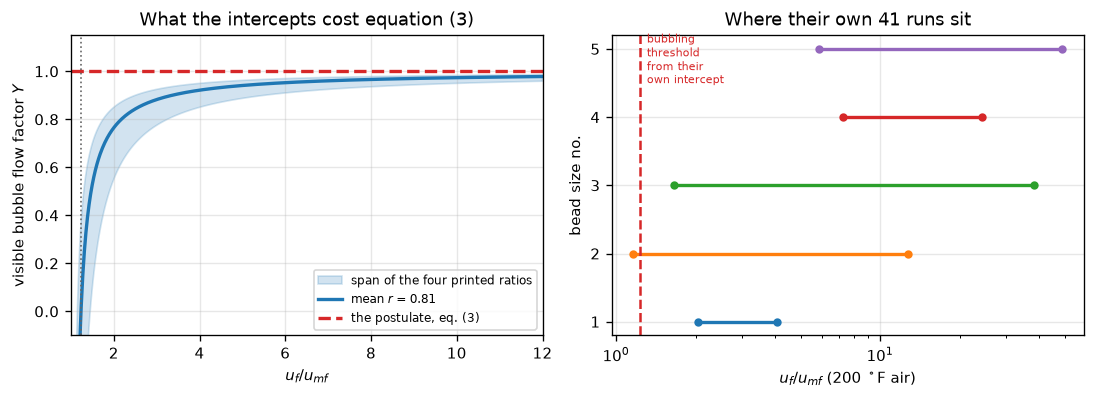

5. Figure 5 without digitising Figure 5

The paper’s Figure 5 plots \(\Delta P_{ke}/L\) against \(u_p/D_p^{0.5}\) and claims

“Here again the square root of the particle diameter correlates the data on velocities within a fluidized system.”

Both axes are columns of Table 3, so the figure needs no digitising at all, the thirteen points are printed. The claim is that \(D_p^{0.5}\) is the right normaliser, and that is testable by letting the exponent go free.

y5 = t3.dPke_over_L_lb_ft3.to_numpy()
up = t3.up_ft_s.to_numpy()
dpv = np.array([dp_ft[b] for b in t3.bead_no])


def ln_scatter(n, y=y5):
    """Residual standard deviation of ln(dPke/L) against ln(u_p / D_p^n)."""
    xx = np.log(up) - n * np.log(dpv)
    s, c = np.polyfit(xx, np.log(y), 1)
    return float(np.std(np.log(y) - (s * xx + c), ddof=2))


def fig5_fit(y=y5):
    """Free exponent and its one-sigma interval.

    ln y = s ln u_p + m ln D_p + c is linear in (s, m, c), and ln_scatter(n) is
    that fit restricted to m = -s n, so the free optimum is n = -m/s from one
    least-squares solve. The interval is where the scatter has risen by the
    one-sigma factor sqrt(1 + 1/dof): a find_roots scan over n in [-3, 6] must
    return exactly two crossings."""
    A = np.column_stack([np.log(up), np.log(dpv), np.ones_like(up)])
    (s, m, _), *_ = np.linalg.lstsq(A, np.log(y), rcond=None)
    n_best = float(-m / s)
    sc_best = ln_scatter(n_best, y)
    thr = sc_best * np.sqrt(1.0 + 1.0 / (len(y) - 3))
    r = find_roots(lambda n: ln_scatter(n, y) - thr, -3.0, 6.0, n_scan=64)
    if len(r["roots"]) != 2 or r["failed"]:
        raise ValueError(f"expected two crossings of the one-sigma level: {r['message']}")
    return n_best, sc_best, float(r["roots"][0]), float(r["roots"][1])


N_BEST, SC_BEST, FIG5_N_LO, FIG5_N_HI = fig5_fit()
SC_HALF, SC_NULL = ln_scatter(0.5), ln_scatter(0.0)
slope5, icpt5 = np.polyfit(np.log(up) - 0.5 * np.log(dpv), np.log(y5), 1)
FIG5_NULL_GAIN = float(SC_NULL / SC_HALF)
FIG5_HALF_COST = float(SC_HALF / SC_BEST - 1)
print(f"exponent n on D_p, free      : {N_BEST:.4f}   scatter {SC_BEST:.4f}")
print(f"n = 0.5, the paper's claim   : scatter {SC_HALF:.4f}  "
      f"({FIG5_HALF_COST:+.2%} worse than the optimum)")
print(f"n = 0,   no normalisation    : scatter {SC_NULL:.4f}   <-- NULL BASELINE "
      f"({FIG5_NULL_GAIN - 1:.0%} worse than n = 0.5)")
print(f"1-sigma interval on n        : [{FIG5_N_LO:.3f}, {FIG5_N_HI:.3f}]   "
      f"({len(y5)} points, {t3.bead_no.nunique()} bead sizes)")
print(f"\nfitted Figure 5 line at n = 0.5: "
      f"dPke/L = {np.exp(icpt5):.4f} (u_p/D_p^0.5)^{slope5:.4f}")
print(f"worst point off that line     : factor "
      f"{np.exp(np.abs(np.log(y5) - (slope5 * (np.log(up) - 0.5 * np.log(dpv)) + icpt5)).max()):.3f}")

claims.value("fig5_null_gain", FIG5_NULL_GAIN)
claims.value("fig5_n_best", N_BEST)
claims.value("fig5_half_cost", FIG5_HALF_COST)
claims.value("fig5_n_interval_lo", FIG5_N_LO)
claims.value("fig5_n_interval_hi", FIG5_N_HI)
claims.value("fig5_n_interval_width", FIG5_N_HI - FIG5_N_LO)
brk("Figure 5 exponent moved 0.5 -> 1.5", "fig5_null_gain", SC_NULL / ln_scatter(1.5))
_i5 = int(np.flatnonzero((t3.bead_no.to_numpy() == 3) & (t3.G_lb_hr_ft2.to_numpy() == 66))[0])
_y5 = y5.copy(); _y5[_i5] *= 1.3
_f5 = fig5_fit(_y5)
_lab5 = f"Table 3 dPke/L of bead 3 at G = 66 raised 30 % ({y5[_i5]} -> {_y5[_i5]:.3f})"
_i2 = int(np.flatnonzero((t3.bead_no.to_numpy() == 2) & (t3.G_lb_hr_ft2.to_numpy() == 737))[0])
_y2 = y5.copy(); _y2[_i2] *= 1.3
brk(f"Table 3 dPke/L of bead 2 at G = 737 raised 30 % ({y5[_i2]} -> {_y2[_i2]:.3f})", "fig5_n_best",
    fig5_fit(_y2)[0])
brk(_lab5, "fig5_half_cost", ln_scatter(0.5, _y5) / _f5[1] - 1)
brk(_lab5, "fig5_n_interval_lo", _f5[2])
brk(_lab5, "fig5_n_interval_hi", _f5[3])
brk(_lab5, "fig5_n_interval_width", _f5[3] - _f5[2])

exponent n on D_p, free      : 0.6173   scatter 0.2231
n = 0.5, the paper's claim   : scatter 0.2301  (+3.14% worse than the optimum)
n = 0,   no normalisation    : scatter 0.3568   <-- NULL BASELINE (55% worse than n = 0.5)
1-sigma interval on n        : [0.470, 0.766]   (13 points, 3 bead sizes)

fitted Figure 5 line at n = 0.5: dPke/L = 0.8234 (u_p/D_p^0.5)^0.8365
worst point off that line     : factor 1.569

True

The claim survives in the weak sense and fails in the strong one. Normalising by \(D_p^{0.5}\) does help: it cuts the log scatter by a third against not normalising at all, so the square root is doing real work. But the data cannot tell \(D_p^{0.5}\) from the free optimum: the one-sigma interval on the exponent, [0.47, 0.77], contains 0.5 comfortably and the paper’s value costs 3 % in scatter. But that interval is narrower than it looks, because with three bead sizes and thirteen points a per-bead offset and a power of \(D_p\) are nearly the same degree of freedom, the exponent is mostly being asked to line up three groups, not to resolve a physical scaling. “The square root of the particle diameter correlates the data” is supported. Why it should be the square root is not tested by Figure 5, and it is worth noting that the same three-point degeneracy is why the collapse metric could not have caught the bead-2 defect found above.

5b. The one column nothing else on this page can see

Table 3’s \(\Delta P_{ke}/L\), thirteen values hand-read off a microfilm scan, enters this page in exactly one place, as Figure 5’s ordinate, and fig5_null_gain is the only metric that touches it. That metric turns out to be a poor guard on it: the cell below corrupts each value in turn by \(+30\) % and measures the drift.

There is, however, a second printing of the same physical quantity. Table 2 prints \(\Delta P_{ke}/\Delta P_{mf}\) for the runs whose cells are legible, and Table 2 also prints \(\Delta P_{mf}\) and \(L_{mf}\) for those runs, so

\[\frac{\Delta P_{ke}}{\Delta P_{mf}} \;=\; \frac{\Delta P_{ke}/L}{\Delta P_{mf}/L_{mf}} \qquad\text{if the } L \text{ of Table 3 is } L_{mf},\]

which is a comparison between two independently typeset columns of two different tables. It is the check the \(\Delta P_{ke}/L\) column otherwise does not have, and it is also the partial recovery of the illegible \(\Delta P_{ke}/\Delta P_{mf}\) cells that the dataset sidecar refers to, computed here rather than asserted.

# ---- (a) can fig5_null_gain see a wrong dPke/L cell?  Corrupt each in turn.
_drift = []
for i in range(len(y5)):
    yy = y5.copy(); yy[i] *= 1.30
    _drift.append(ln_scatter(0.0, yy) / ln_scatter(0.5, yy) / FIG5_NULL_GAIN - 1.0)
_drift = np.array(_drift)
FIG5_MEDIAN_CELL_DRIFT = float(np.median(np.abs(_drift)))
print("drift in fig5_null_gain when ONE dPke/L cell is raised 30 %:")
print(pd.DataFrame(dict(bead=t3.bead_no.astype(int), G=t3.G_lb_hr_ft2, drift=_drift))
      .to_string(index=False, float_format=lambda v: f"{v:10.4f}"))
print(f"median |drift| {FIG5_MEDIAN_CELL_DRIFT:.2%}; "
      f"{int((np.abs(_drift) < claims.metrics['fig5_null_gain']['rtol']).sum())} of {len(_drift)} "
      f"sit inside the claim's own {claims.metrics['fig5_null_gain']['rtol']:.0%} tolerance")

# ---- (b) the cross-check, against Table 2's legible ratio column
cross = []
for _, r in t3.iterrows():
    m = t2[(t2.bead_no == r.bead_no) & (np.abs(t2.G_lb_hr_ft2 - r.G_lb_hr_ft2) <= 0.5)
           & t2.dPke_over_dPmf.notna()]
    if len(m) != 1:                    # ambiguous or illegible: no comparison exists
        print(f"  no comparison for bead {int(r.bead_no)} at G = {r.G_lb_hr_ft2:.0f}: "
              f"{len(m)} legible Table-2 rows match")
        continue
    q = m.iloc[0]
    w_run = q.dPmf_inH2O * INH2O / (q.Lmf_in * IN)                   # Pa/m
    inferred = r.dPke_over_L_lb_ft3 * LBF_FT2 / FT / w_run           # lbf/ft3 -> Pa/m
    cross.append(dict(bead=int(r.bead_no), G=r.G_lb_hr_ft2,
                      dPke_over_L=r.dPke_over_L_lb_ft3,
                      inferred_ratio=inferred, printed_ratio=q.dPke_over_dPmf,
                      dev=inferred / q.dPke_over_dPmf - 1.0))
cross = pd.DataFrame(cross)
print()
print(cross.to_string(index=False, float_format=lambda v: f"{v:12.5f}"))


def dpke_cross(bump=None, factor=1.30):
    """(RMS, worst |deviation|) between Table 3's dPke/L and Table 2's legible
    ratio column; ``bump`` = (bead, G) corrupts ONE dPke/L cell by ``factor``."""
    d = cross.dev.to_numpy().copy()
    if bump is not None:
        i = int(np.flatnonzero((cross.bead.to_numpy() == bump[0]) & (cross.G.to_numpy() == bump[1]))[0])
        d[i] = (1.0 + d[i]) * factor - 1.0
    return float(np.sqrt((d ** 2).mean())), float(np.abs(d).max())


DPKE_CROSS_RMS, DPKE_CROSS_WORST = dpke_cross()
print(f"\n{len(cross)} runs where BOTH columns are legible and the match is unambiguous")
print(f"  median |deviation| {np.median(cross.dev.abs()):.2%}, worst {DPKE_CROSS_WORST:.2%}, "
      f"RMS {DPKE_CROSS_RMS:.2%}")
print(f"  mean signed deviation {cross.dev.mean():+.2%}: centred, not offset, which is what "
      f"decides\n  that the L of Table 3 is L_mf and not the expanded L_f (section 6 puts a "
      f"number on that offset)")
claims.value("dPke_cross_check_rms", DPKE_CROSS_RMS)
claims.value("dPke_cross_check_worst", DPKE_CROSS_WORST)
for _bg in [(4, 103), (3, 272)]:
    brk(f"Table 3 dPke/L of bead {_bg[0]} at G = {_bg[1]} raised 30 %", "dPke_cross_check_rms",
        dpke_cross(_bg)[0])
_bw = tuple(cross.loc[cross.dev.abs().idxmax(), ["bead", "G"]])
brk(f"Table 3 dPke/L of bead {int(_bw[0])} at G = {_bw[1]:.0f} raised 30 %",
    "dPke_cross_check_worst", dpke_cross((_bw[0], _bw[1]))[1])

drift in fig5_null_gain when ONE dPke/L cell is raised 30 %:
 bead   G      drift
    2 737    -0.0774
    2 613    -0.0536
    2 270    -0.0166
    2 141     0.0352
    3 747    -0.0608
    3 345    -0.0118
    3 272    -0.0184
    3  66    -0.1228
    4 346     0.0007
    4 201     0.0112
    4 155    -0.0026
    4 127     0.0883
    4 103    -0.0491
median |drift| 3.52%; 8 of 13 sit inside the claim's own 5% tolerance
  no comparison for bead 2 at G = 737: 2 legible Table-2 rows match
  no comparison for bead 2 at G = 141: 0 legible Table-2 rows match
  no comparison for bead 4 at G = 346: 0 legible Table-2 rows match

 bead   G  dPke_over_L  inferred_ratio  printed_ratio          dev
    2 613     28.50000         0.26854        0.27800     -0.03401
    2 270     14.20000         0.13357        0.17700     -0.24536
    3 747     34.70000         0.33555        0.34900     -0.03855
    3 345     25.60000         0.24786        0.24300      0.01999
    3 272     22.70000         0.21933        0.20400      0.07513
    3  66      5.88000         0.05693        0.05410      0.05230
    4 201     17.20000         0.17094        0.17900     -0.04502
    4 155     15.60000         0.15504        0.16400     -0.05463
    4 127     14.30000         0.14212        0.13500      0.05274
    4 103     12.90000         0.12821        0.11700      0.09578

10 runs where BOTH columns are legible and the match is unambiguous
  median |deviation| 5.25%, worst 24.54%, RMS 9.41%
  mean signed deviation -1.22%: centred, not offset, which is what decides
  that the L of Table 3 is L_mf and not the expanded L_f (section 6 puts a number on that offset)

True

What the cross-check says. The two columns agree to a few per cent in the median, with one run several times worse, good enough to call the \(\Delta P_{ke}/L\) column corroborated, not good enough to recover the illegible \(\Delta P_{ke}/\Delta P_{mf}\) cells as data, which is why those cells stay empty in the CSV. The deviations scatter about zero, which is itself informative: had Table 3’s \(L\) meant the expanded height \(L_f\), every inferred ratio would be high by the expansion ratio computed in section 6 (about a fifth), and they are not.

dPke_cross_check_rms is a claim on this page for one reason: it is the only number on this page that a transcription error in the \(\Delta P_{ke}/L\) column has to move. The break table injects exactly that.

6. What the pressure drop does to the superficial velocity

Now the pymrm solve. The reference case is bead size 3 at its lowest bubbling run, \(\Delta P_{mf} = 40.7\) in. H₂O, \(L_{mf} = 24.6\) in., \(G = 66.0\) lb/(hr)(ft²), because that is a deep bed near the bubbling threshold, which is where the Figure-3 intercept is read and where equation (1) is still inside its range.

BEAD_REF = 3
ref = t2[(t2.bead_no == BEAD_REF) & (t2.G_lb_hr_ft2 == 66.0)].iloc[0]
w_mf   = ref.dPmf_inH2O * INH2O / (ref.Lmf_in * IN)
L_mf   = ref.Lmf_in * IN
dp_ref = float(t1[t1.bead_no == BEAD_REF].dp_micron.iloc[0]) * 1e-6
a_exp  = PRINTED["eq1_coefficient"] / np.sqrt(dp_ref / FT) / FT        # s/m
u_mf   = PRINTED[f"Re_mf_bead{BEAD_REF}"] * mu_air(T_PAPER) / (dp_ref * rho_air(T_PAPER))
u_e_meas = u_mf / R_MEAN
u_top  = ref.G_lb_hr_ft2 * G_SI / rho_air(T_PAPER)
P_BOT  = PATM + w_mf * L_mf
PRESSURE_RATIO = P_BOT / PATM
_deep = t2.loc[t2.dPmf_inH2O.idxmax()]

print(f"deepest pressure drop in Table 2: bead {int(_deep.bead_no)}, {_deep.dPmf_inH2O} in.H2O over "
      f"L_mf = {_deep.Lmf_in} in.")
print(f"bed weight w_mf      = {w_mf:9.1f} Pa/m   (= {ref.dPmf_inH2O} in.H2O / {ref.Lmf_in} in.)")
print(f"L_mf                 = {L_mf:9.5f} m      P_bot/P_top = {PRESSURE_RATIO:.5f}")
print(f"u_mf  (from Re = {PRINTED[f'Re_mf_bead{BEAD_REF}']})  = {u_mf:9.5f} m/s")
print(f"u_e   (from r = {R_MEAN:.2f})      = {u_e_meas:9.5f} m/s")
print(f"u_top (from G = {ref.G_lb_hr_ft2})    = {u_top:9.5f} m/s   -> u_top/u_mf = {u_top / u_mf:.4f}")
print(f"a = 0.065/sqrt(D_p) = {a_exp:9.4f} s/m")
print(f"bubble velocity from eq. (4), sqrt(D_p)/0.065 = "
      f"{np.sqrt(dp_ref / FT) / PRINTED['eq1_coefficient']:.4f} ft/s")

deepest pressure drop in Table 2: bead 1, 44.3 in.H2O over L_mf = 25.0 in.
bed weight w_mf      =   16224.8 Pa/m   (= 40.7 in.H2O / 24.6 in.)
L_mf                 =   0.62484 m      P_bot/P_top = 1.10005
u_mf  (from Re = 0.55)  =   0.05593 m/s
u_e   (from r = 0.81)      =   0.06905 m/s
u_top (from G = 66.0)    =   0.09294 m/s   -> u_top/u_mf = 1.6617
a = 0.065/sqrt(D_p) =    7.9558 s/m
bubble velocity from eq. (4), sqrt(D_p)/0.065 = 0.4124 ft/s

N_REF = 1600


def reference_bed(T=T_PAPER, r=R_MEAN, a=a_exp, n=N_REF, x=None, **kw):
    """The reference run (bead 3, G = 66) at air temperature T, u_e = u_mf/r.

    ``x`` replaces the surface velocity by x u_mf; ``kw`` goes to CompressibleBed
    (P_top, v, P_inlet). Returns the bed and u_mf at T."""
    umf_T = PRINTED[f"Re_mf_bead{BEAD_REF}"] * mu_air(T) / (dp_ref * rho_air(T))
    ut = ref.G_lb_hr_ft2 * G_SI / rho_air(T) if x is None else x * umf_T
    return CompressibleBed(w_mf, a, umf_T / r, ut, L_mf, n=n, **kw), umf_T


def pymrm_results(xtol=1e-13, at="faces", **kw):
    """Bed height, profile and excess-velocity spread from the pymrm solve."""
    bd, umf = reference_bed(**kw)
    Lf = bd.Lf(xtol=xtol)
    s = bd.solve(Lf)
    return dict(bed=bd, u_mf=umf, Lf=Lf, sol=s, Lf_over_Lmf=Lf / L_mf,
                spread=bd.excess_spread(s, umf, at=at))


def eq1_single_uf(a=a_exp, r=R_MEAN):
    """L_f/L_mf from equation (1) with the single surface velocity u_top."""
    return 1.0 / (1.0 - a * (u_top - u_mf / r))


R200 = pymrm_results()
bed, sol, Lf_pymrm = R200["bed"], R200["sol"], R200["Lf"]
Lf_exact, Lf_ivp = bed.Lf_analytic(), bed.Lf_ivp()
EXCESS_SPREAD = R200["spread"]
EXCESS_EXACT = float((u_top - u_top * PATM / bed.P_bottom_exact()) / bed.mean_excess_velocity(u_mf))
LF_OVER_LMF = R200["Lf_over_Lmf"]
d_incompressible = a_exp * (u_top - u_e_meas)
LF_INCOMPRESSIBLE = eq1_single_uf()
EQ1_OVERPREDICTION = float(LF_INCOMPRESSIBLE / LF_OVER_LMF - 1.0)
FACE_GAP = abs(sol["P_bottom"] - bed.P_bottom_exact()) / (w_mf * L_mf)
d_top, d_bot = bed.delta(sol["P_surface"]), bed.delta(sol["P_bottom"])
u_bot = u_top * PATM / sol["P_bottom"]

print(f"L_f  pymrm (n={N_REF}) = {Lf_pymrm / IN:.6f} in")
print(f"L_f  closed form    = {Lf_exact / IN:.6f} in")
print(f"L_f  solve_ivp      = {Lf_ivp / IN:.6f} in")
print(f"     closed form vs solve_ivp : below 1e-10 (here {abs(Lf_exact - Lf_ivp) / Lf_exact:.1e}); "
      f"the same end condition P(L_f) = P_top + w L_mf, integrated two ways")
print(f"     pymrm vs closed form     : {abs(Lf_pymrm - Lf_exact) / Lf_exact:.3e}")
print(f"distributor face pressure from compute_boundary_values minus P_top + w L_mf: "
      f"below 1e-9 of the bed pressure drop (here {FACE_GAP:.1e})")
print(f"\nL_f/L_mf compressible  = {LF_OVER_LMF:.5f}")
print(f"L_f/L_mf from eq. (1) with a single u_f = {LF_INCOMPRESSIBLE:.5f} "
      f"({EQ1_OVERPREDICTION:+.2%})")
print(f"\ndelta at the surface face     = {d_top:.5f}")
print(f"delta at the distributor face = {d_bot:.5f}   ratio {d_top / d_bot:.4f}")
print(f"(u_f - u_mf) surface {u_top - u_mf:.6f}  distributor {u_bot - u_mf:.6f}  "
      f"depth average {bed.mean_excess_velocity(u_mf):.6f} m/s")
print(f"  => the quantity in equation (3) varies by {EXCESS_SPREAD:.2%} across this bed "
      f"(face values; {EXCESS_EXACT:.2%} by quadrature of the closed form)")
print(f"Newton iterations at the root: {sol['nit']}")
print(f"\nexpansion ratio L_f/L_mf = {LF_OVER_LMF:.5f}: had Table 3's L meant L_f, the "
      f"inferred\n  dPke/dPmf of section 5b would all be {LF_OVER_LMF - 1:+.1%} high, and the "
      f"measured mean deviation is {cross.dev.mean():+.2%}. So L there is L_mf.")

claims.value("Lf_over_Lmf", LF_OVER_LMF)
claims.value("eq1_overprediction", EQ1_OVERPREDICTION)
claims.value("excess_velocity_spread", EXCESS_SPREAD)
claims.value("pymrm_vs_closed_form", abs(Lf_pymrm - Lf_exact) / Lf_exact,
             note=f"first-order upwind at n = {N_REF}")
claims.bound("closed_form_vs_ivp", abs(Lf_exact - Lf_ivp) / Lf_exact, max=1e-10,
             basis="tolerance", note="solve_ivp rtol 1e-12")
claims.bound("distributor_face_identity", FACE_GAP, max=1e-9, basis="tolerance",
             note="summing the upwind equations gives P_bottom - P_inlet = w L_f (1 - mean delta), "
                  "which the inventory root sets to w L_mf; Newton and root tolerances")

L_f  pymrm (n=1600) = 29.139485 in
L_f  closed form    = 29.140211 in
L_f  solve_ivp      = 29.140211 in
     closed form vs solve_ivp : below 1e-10 (here 6.6e-13); the same end condition P(L_f) = P_top + w L_mf, integrated two ways
     pymrm vs closed form     : 2.492e-05
distributor face pressure from compute_boundary_values minus P_top + w L_mf: below 1e-9 of the bed pressure drop (here 1.9e-14)

L_f/L_mf compressible  = 1.18453
L_f/L_mf from eq. (1) with a single u_f = 1.23465 (+4.23%)

delta at the surface face     = 0.19005
delta at the distributor face = 0.12280   ratio 1.5476
(u_f - u_mf) surface 0.037007  distributor 0.028555  depth average 0.032703 m/s
  => the quantity in equation (3) varies by 25.85% across this bed (face values; 25.85% by quadrature of the closed form)
Newton iterations at the root: 4

expansion ratio L_f/L_mf = 1.18453: had Table 3's L meant L_f, the inferred
  dPke/dPmf of section 5b would all be +18.5% high, and the measured mean deviation is -1.22%. So L there is L_mf.

# ---- the 70 F counterpart the Parameters section promises for EVERY velocity ratio.
# Only the gas properties change; the bed weight and eq. (1) do not depend on T.
R70 = pymrm_results(T=T_ROOM)
EXCESS_SPREAD_70F, LF_OVER_LMF_70F = R70["spread"], R70["Lf_over_Lmf"]
u_top_70 = R70["bed"].u_top
print(f"                                        200 F        70 F")
print(f"u_f/u_mf at the surface           {u_top / u_mf:11.4f} {u_top_70 / R70['u_mf']:11.4f}")
print(f"excess-velocity spread across bed {EXCESS_SPREAD:11.4%} {EXCESS_SPREAD_70F:11.4%}")
print(f"L_f/L_mf                          {LF_OVER_LMF:11.5f} {LF_OVER_LMF_70F:11.5f}")
claims.value("excess_velocity_spread_70F", EXCESS_SPREAD_70F)
claims.value("Lf_over_Lmf_70F", LF_OVER_LMF_70F)
N_ABOVE_ADD = claims.count("spreads_above_additive_shortfall", [EXCESS_SPREAD, EXCESS_SPREAD_70F],
                           SHORTFALL_ADD, min_margin=0.02)
N_ABOVE_MUL = claims.count("spreads_above_multiplicative_shortfall",
                           [EXCESS_SPREAD, EXCESS_SPREAD_70F], SHORTFALL_MUL, min_margin=0.02)
print(f"\n{N_ABOVE_ADD} of 2 exceed the shortfall the intercepts report on the additive reading, "
      f"1 - u_mf/u_e = {SHORTFALL_ADD:.1%};")
print(f"on the multiplicative reading, u_e/u_mf - 1 = {SHORTFALL_MUL:.1%}, {N_ABOVE_MUL} of 2 "
      f"(the 200 F figure) does.")
print("This page means the additive reading, and says so wherever the comparison is made.")

                                        200 F        70 F
u_f/u_mf at the surface                1.6617      1.9598
excess-velocity spread across bed    25.8472%    20.5159%
L_f/L_mf                              1.18453     1.23780

2 of 2 exceed the shortfall the intercepts report on the additive reading, 1 - u_mf/u_e = 19.0%;
on the multiplicative reading, u_e/u_mf - 1 = 23.5%, 1 of 2 (the 200 F figure) does.
This page means the additive reading, and says so wherever the comparison is made.

# the partial-bubbling window: bubbling at the top, none at the bottom
WIN_LO = 1.0 / R_MEAN
WIN_HI = PRESSURE_RATIO / R_MEAN
WINDOW_WIDTH = float(WIN_HI / WIN_LO - 1.0)
print(f"partial-bubbling window in u_f/u_mf (u_f read at the SURFACE): "
      f"[{WIN_LO:.4f}, {WIN_HI:.4f}]")
print(f"width {WINDOW_WIDTH:.2%}: exactly the bed's own pressure ratio, P_bot/P_top - 1 = "
      f"{PRESSURE_RATIO - 1:.2%}\n")


def partial_fraction(x=1.30, **kw):
    """Non-bubbling bottom fraction of the bed at a fixed u_f/u_mf = x (closed form)."""
    bd, _ = reference_bed(x=x, **kw)
    Ps, Lf_b = bd.P_switch(), bd.Lf_analytic()
    if Ps <= bd.P_top:                                # u <= u_e even at the surface
        return 1.0
    if Ps >= bd.P_bottom_exact():                     # u > u_e even at the distributor
        return 0.0
    return float(1.0 - bd.s_analytic(Ps) / Lf_b)


def branch_table(n=N_REF):
    rows = []
    for label, x in [("no bubbles anywhere", 1.15), ("at the lower switch", WIN_LO),
                     ("partial, window midpoint", 0.5 * (WIN_LO + WIN_HI)),
                     ("partial, fixed u_f/u_mf = 1.30", 1.30),
                     ("at the upper switch", WIN_HI), ("bubbling throughout", 1.66)]:
        bd, _ = reference_bed(x=x, n=n)
        Lf_b = bd.Lf_analytic()
        Lf_n = bd.Lf()
        rows.append(dict(case=label, u_over_umf=x, Lf_over_Lmf=Lf_b / L_mf,
                         non_bubbling_bottom_fraction=partial_fraction(x),
                         delta_mean=bd.solve(Lf_n)["delta"].mean(),
                         pymrm_vs_exact=abs(Lf_n - Lf_b) / Lf_b))
    return pd.DataFrame(rows)


branches = branch_table()
print(branches.to_string(index=False, float_format=lambda v: f"{v:14.6f}"))
PARTIAL_FRACTION = partial_fraction(1.30)
BRANCH_WORST = float(branches.pymrm_vs_exact.max())
print(f"\nboth branches and both switches solved at n = {N_REF}; worst pymrm-vs-exact "
      f"{BRANCH_WORST:.3e}")
claims.value("partial_bubbling_fraction_at_1p30", PARTIAL_FRACTION)
claims.value("partial_bubbling_window_width", WINDOW_WIDTH)
claims.value("shortfall_additive", SHORTFALL_ADD, note="1 - u_mf/u_e at the mean printed ratio")
claims.value("shortfall_multiplicative", SHORTFALL_MUL, note="u_e/u_mf - 1 at the mean printed ratio")
claims.value("window_lower_switch", WIN_LO, note="u_f/u_mf at the surface where bubbling starts")
claims.value("window_upper_switch", WIN_HI, note="u_f/u_mf at the surface where the bottom bubbles too")
_rf = 1.0                                           # the postulate: u_mf/u_e = 1
for _m, _b in (("shortfall_additive", 1.0 - _rf), ("shortfall_multiplicative", 1.0 / _rf - 1.0),
               ("window_lower_switch", 1.0 / _rf), ("window_upper_switch", PRESSURE_RATIO / _rf)):
    brk("u_mf/u_e forced to 1.0 (the postulate itself)", _m, _b)
claims.value("branch_worst_pymrm_vs_exact", BRANCH_WORST, note=f"first-order upwind at n = {N_REF}")
brk("u_mf/u_e forced to 1.0 (the postulate itself)", "partial_bubbling_fraction_at_1p30",
    partial_fraction(1.30, r=1.0))
brk(f"atmospheric datum x10 (bed pressure ratio {PRESSURE_RATIO:.3f} -> "
    f"{1 + w_mf * L_mf / (10 * PATM):.3f})", "partial_bubbling_fraction_at_1p30",
    partial_fraction(1.30, P_top=10 * PATM))
brk(f"atmospheric datum x10 (bed pressure ratio {PRESSURE_RATIO:.3f} -> "
    f"{1 + w_mf * L_mf / (10 * PATM):.3f})", "partial_bubbling_window_width",
    w_mf * L_mf / (10 * PATM))
brk("branch table on n = 50", "branch_worst_pymrm_vs_exact",
    float(branch_table(50).pymrm_vs_exact.max()))

partial-bubbling window in u_f/u_mf (u_f read at the SURFACE): [1.2346, 1.3581]
width 10.01%: exactly the bed's own pressure ratio, P_bot/P_top - 1 = 10.01%

                          case     u_over_umf    Lf_over_Lmf  non_bubbling_bottom_fraction     delta_mean  pymrm_vs_exact
           no bubbles anywhere       1.150000       1.000000                      1.000000       0.000000        0.000000
           at the lower switch       1.234568       1.000000                      1.000000       0.000000        0.000000
      partial, window midpoint       1.296329       1.006884                      0.496582       0.006828        0.000009
partial, fixed u_f/u_mf = 1.30       1.300000       1.007727                      0.466677       0.007659        0.000009
           at the upper switch       1.358091       1.027608                      0.000000       0.026849        0.000018
           bubbling throughout       1.660000       1.183550                      0.000000       0.155063        0.000025

both branches and both switches solved at n = 1600; worst pymrm-vs-exact 2.488e-05

True

fig, ax = plt.subplots(1, 3, figsize=(10.5, 3.2))
s_ref = bed.x_c.ravel() * Lf_pymrm / IN
u_z = u_top * PATM / sol["P"]
ax[0].plot(sol["P"] / 1000, s_ref, "C0")
ax[0].invert_yaxis(); ax[0].set_xlabel("$P$, kPa"); ax[0].set_ylabel("depth below surface $s$, in.")
ax[0].set_title("pressure")
ax[1].plot(u_z / u_mf, s_ref, "C0", label=r"$u_f/u_{mf}$")
ax[1].axvline(u_e_meas / u_mf, color="C1", ls="--", label=r"$u_e/u_{mf}$, measured")
ax[1].axvline(1.0, color="C3", ls=":", label=r"$u_{mf}$, the postulate")
ax[1].invert_yaxis(); ax[1].set_xlabel(r"$u/u_{mf}$, -"); ax[1].set_title("superficial velocity")
ax[1].legend(fontsize=7)
ax[2].plot(sol["delta"], s_ref, "C0")
ax[2].axvline(d_incompressible, color="C3", ls="--",
              label="eq. (1) with a single $u_f$")
ax[2].invert_yaxis(); ax[2].set_xlabel(r"bubble fraction $\delta$, -")
ax[2].set_title("expansion"); ax[2].legend(fontsize=7)
plt.show()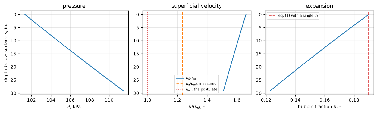

Three statements, all from the paper’s own measured bed weight.

1. The quantity equation (3) is written in, the excess velocity \(u_f - u_{mf}\), is not a number. It varies by about a quarter between distributor and surface in this deep bed at 200 °F, and by about a fifth at 70 °F, larger, at both assumed air temperatures, than the shortfall the intercepts report, where “shortfall” means \(1 - u_{mf}/u_e\), the additive reading printed above. (On the multiplicative reading \(u_e/u_{mf} - 1\) the 70 °F figure is the smaller of the two; the page states the additive comparison so that the claim cannot be read two ways.) Any test of the postulate that does not say where \(u_f\) is evaluated has an uncertainty of that size built in.
2. Applying equation (1) with a single \(u_f\), as the paper does, over-predicts the expansion. The error grows with velocity because \(\delta\) is nonlinear in \(u\).
3. There is a band of superficial velocities, exactly as wide as the bed’s own pressure ratio, in which the top of the bed bubbles and the bottom does not. That band sits astride the bubbling threshold, which is where the Figure-3 intercepts are extrapolated to. It is the curvature the authors predict and never compute, and it is entirely a compressibility effect.

7. Where equation (4) stops meaning anything

One more internal check, and it is the sharpest limit on the paper’s own logic. Equation (1) is linear in \((u_f - u_{mf})\), so \(\delta = 1\), a bed of pure bubbles, at a finite velocity. That velocity is \(D_p^{0.5}/0.065\), which is also the bubble velocity equation (4) deduces. The two are the same number because \(u_b = (u_f-u_{mf})/\delta\).

def eq4_limits(coeff=PRINTED["eq1_coefficient"]):
    """Per bead: eq. (4)'s bubble velocity, the velocity at which eq. (1) gives
    delta = 1, and how far Table 2's fastest run goes past it."""
    rows = []
    for b in sorted(t1.bead_no):
        dpb = float(t1[t1.bead_no == b].dp_micron.iloc[0]) * 1e-6
        ub_ft = np.sqrt(dpb / FT) / coeff                               # ft/s, eq. (4)
        umf_b = PRINTED[f"Re_mf_bead{b}"] * mu_air(T_PAPER) / (dpb * rho_air(T_PAPER))
        x_hi = excess_ratio(t2[t2.bead_no == b].G_lb_hr_ft2.max(), b, T_PAPER)
        rows.append(dict(bead=int(b), u_b_eq4_ft_s=ub_ft, u_mf_ft_s=umf_b / FT,
                         u_at_delta_1_over_umf=1 + ub_ft * FT / umf_b,
                         max_run_u_over_umf=x_hi, overshoot=x_hi / (1 + ub_ft * FT / umf_b)))
    return pd.DataFrame(rows)


def wall_vs_bubble(coeff=PRINTED["eq1_coefficient"]):
    """Measured wall particle velocity against eq. (4)'s bubble velocity."""
    lim_ = eq4_limits(coeff).set_index("bead")
    up_max = t3.groupby("bead_no").up_ft_s.max()
    return pd.DataFrame([dict(bead=int(b), u_b_eq4_ft_s=lim_.u_b_eq4_ft_s[b],
                              u_p_max_measured_ft_s=float(up_max[b]),
                              ratio=float(up_max[b]) / lim_.u_b_eq4_ft_s[b]) for b in up_max.index])


lim = eq4_limits()
print(lim.to_string(index=False, float_format=lambda v: f"{v:14.4f}"))
EQ1_OVERSHOOT = float(lim.overshoot.max())
print(f"\nTable 2 pushes eq. (1) up to {EQ1_OVERSHOOT:.1f}x past the velocity at which it "
      f"predicts a bed of pure bubbles")
cmp = wall_vs_bubble()
print("\nmeasured wall particle velocity against the bubble velocity eq. (4) deduces:")
print(cmp.to_string(index=False, float_format=lambda v: f"{v:12.4f}"))
UP_OVER_UB = float(cmp.ratio.max())
print(f"\nparticles at the wall move up to {UP_OVER_UB:.2f}x faster than the bubbles that "
      f"are supposed to be dragging them")
claims.value("eq1_overshoot", EQ1_OVERSHOOT)
claims.value("up_over_ub_eq4", UP_OVER_UB,
             note="exactly linear in eq. (1)'s coefficient, so its break row only rescales it")
_c12 = PRINTED["eq1_coefficient"] * 1.2
_lab = f"eq. (1) coefficient {PRINTED['eq1_coefficient']} -> {_c12:.3f} (+20 %)"
brk(_lab, "eq1_overshoot", float(eq4_limits(_c12).overshoot.max()))
brk(_lab, "up_over_ub_eq4", float(wall_vs_bubble(_c12).ratio.max()))

 bead   u_b_eq4_ft_s      u_mf_ft_s  u_at_delta_1_over_umf  max_run_u_over_umf      overshoot
    1         0.8115         1.0511                 1.7720              4.0830         2.3042
    2         0.5403         0.5596                 1.9655             12.7294         6.4762
    3         0.4124         0.1835                 3.2474             38.2694        11.7845
    4         0.2869         0.0655                 5.3815             24.4110         4.5361
    5         0.2067         0.0186                12.1122             48.9359         4.0402

Table 2 pushes eq. (1) up to 11.8x past the velocity at which it predicts a bed of pure bubbles

measured wall particle velocity against the bubble velocity eq. (4) deduces:
 bead  u_b_eq4_ft_s  u_p_max_measured_ft_s        ratio
    2        0.5403                 2.4600       4.5526
    3        0.4124                 1.8400       4.4619
    4        0.2869                 0.8300       2.8930

particles at the wall move up to 4.55x faster than the bubbles that are supposed to be dragging them

True

Equation (4) is the paper’s cleanest-looking result, a bubble velocity that depends on nothing but particle size. It is obtained by dividing an expansion correlation by the postulate, and the expansion correlation is linear, so it is only meaningful while \(\delta \ll 1\). Table 2’s own runs go an order of magnitude past the point where it predicts \(\delta = 1\). And the paper’s own Fastax measurements have particles at the wall moving several times faster than the bubbles equation (4) gives, which the authors touch on and never quantify. Their sentence, quoted exactly, is about the number of collisions, not the bubble velocity:

“The dependence of the velocity of the discontinuous phase on \(D_p^{0.5}\) will affect this relationship in two ways. First, as the bubbles rise faster they will move the particles correspondingly faster, and hence the number of collisions from this effect should increase as \(D_p^{0.5}\). This was partially verified by the particle velocity measurements.”

The clause this page needs is the first one, the velocity of the discontinuous phase goes as \(D_p^{0.5}\), which is exactly what equation (4) asserts. The authors then check it against the particle velocities without ever putting the two numbers side by side; the table above does.

Validation

Every number on the page is registered as a claim with how it is checked, and every claim has at least one row in the defect-injection table below that fails the claim’s own check. The rows pass each defect through an argument or a physical parameter of the functions that computed the claim.

The grid ladder and the two validation routes

The finite-volume bed height is compared with the closed form and the Runge-Kutta route of the implementation section on six grids, at both assumed air temperatures. The reported numbers are the \(n = 1600\) values; the observed order and the Richardson extrapolation (pymrm.checks.observed_orders) show that the ladder is in its asymptotic range. The excess-velocity spread from the face values is compared with the same quantity from the closed form, with the depth average of \(u - u_{mf}\) taken by quadrature in \(P\) (\(\int (u-u_{mf})\,\mathrm{d}s = \int (u-u_{mf})/(w_{mf}(1-\delta))\,\mathrm{d}P\)), on every rung. The finest-rung difference is checked against the round-off and root-tolerance floor, so the order is not fitted to noise.

print("--- grid ladder on the pymrm solve (first-order upwind) ---")
NS = (50, 100, 200, 400, 800, 1600)
EPS = np.finfo(float).eps


def ladder(T=T_PAPER, xtol=1e-13, ns=NS):
    """L_f and the face-value excess spread on every rung."""
    return {n: pymrm_results(T=T, n=n, xtol=xtol) for n in ns}


LAD = ladder()
LAD70 = ladder(T_ROOM)
Lf_exact70 = R70["bed"].Lf_analytic()
EXACT70 = float((u_top_70 - u_top_70 * PATM / R70["bed"].P_bottom_exact())
                / R70["bed"].mean_excess_velocity(R70["u_mf"]))
OO = observed_orders(lambda n: LAD[n]["Lf"], NS)
lad = pd.DataFrame(dict(n=NS, Lf_in=[LAD[n]["Lf"] / IN for n in NS],
                        Lf_err_vs_closed_form=[abs(LAD[n]["Lf"] - Lf_exact) / Lf_exact for n in NS],
                        order=[np.nan, np.nan] + list(OO["orders"]),
                        spread_vs_quadrature_200F=[abs(LAD[n]["spread"] - EXCESS_EXACT) for n in NS],
                        spread_vs_quadrature_70F=[abs(LAD70[n]["spread"] - EXACT70) for n in NS],
                        Lf_err_70F=[abs(LAD70[n]["Lf"] - Lf_exact70) / Lf_exact70 for n in NS]))
print(lad.to_string(index=False, float_format=lambda v: f"{v:12.4g}"))
UPWIND_ORDER = float(OO["orders"][-1])
RICH_DEV = float(abs(OO["extrapolated"] - Lf_exact) / Lf_exact)
FINEST = abs(LAD[NS[-1]]["Lf"] - LAD[NS[-2]]["Lf"]) / Lf_exact
FLOOR = max(NS[-1] * EPS, 1e-13 / Lf_exact)        # round-off, and the root tolerance
SPREAD_GAP = max(abs(EXCESS_SPREAD - EXCESS_EXACT), abs(EXCESS_SPREAD_70F - EXACT70))
print(f"\nobserved order (finest triple)       {UPWIND_ORDER:.4f}")
print(f"Richardson limit vs closed form      below 1e-7 (here {RICH_DEV:.1e})")
print(f"finest difference / round-off floor  {FINEST / FLOOR:.1e}")
print(f"spread from face values vs quadrature, worst of 200 F and 70 F at n = {N_REF}: "
      f"below 1e-6 (here {SPREAD_GAP:.1e})")
claims.bound("upwind_order", UPWIND_ORDER, min=0.95, max=1.05, basis="theory",
             note="first-order upwind on a first-order equation")
claims.bound("grid_finest_over_roundoff", FINEST / FLOOR, min=1e3, basis="theory",
             note="finest-rung difference against max(n eps, root tolerance / L_f)")
claims.bound("richardson_vs_closed_form", RICH_DEV, max=1e-7, basis="theory",
             note="second-order remainder of a first-order Richardson extrapolation")
_CELL_GAP = abs(pymrm_results(at="cells")["spread"] - EXCESS_EXACT)
claims.bound("excess_spread_vs_quadrature", SPREAD_GAP, max=1e-6, basis="chosen",
             note="face values and the trapezoidal depth average against quadrature of the "
                  f"closed form; the cell-value reading is {_CELL_GAP:.1e} off")
_lx = {n: pymrm_results(n=n, xtol=1e-4)["Lf"] for n in NS}
_labx = "root tolerance xtol = 1e-4 m on every rung"
brk(f"finest rung solved on n = {NS[-2]} again (refinement not passed)", "upwind_order",
    float(observed_orders(lambda n: LAD[min(n, NS[-2])]["Lf"], NS)["orders"][-1]))
brk(_labx, "grid_finest_over_roundoff",
    abs(_lx[NS[-1]] - _lx[NS[-2]]) / Lf_exact / max(NS[-1] * EPS, 1e-4 / Lf_exact))
_oc = observed_orders(lambda n: pymrm_results(n=n)["Lf"], (25, 50, 100))
brk("Richardson extrapolation from the ladder 25, 50, 100", "richardson_vs_closed_form",
    abs(_oc["extrapolated"] - Lf_exact) / Lf_exact)
brk("spread read at the first and last cell values with a cell mean (at='cells')",
    "excess_spread_vs_quadrature", _CELL_GAP)

--- grid ladder on the pymrm solve (first-order upwind) ---
   n        Lf_in  Lf_err_vs_closed_form        order  spread_vs_quadrature_200F  spread_vs_quadrature_70F   Lf_err_70F
  50        29.12              0.0007967          NaN                  5.997e-07                 2.737e-07    0.0006684
 100        29.13              0.0003986          NaN                  3.617e-07                 1.803e-07    0.0003344
 200        29.13              0.0001993       0.9987                  1.963e-07                  1.01e-07    0.0001672
 400        29.14              9.969e-05       0.9994                   1.02e-07                 5.324e-08    8.362e-05
 800        29.14              4.985e-05       0.9997                  5.197e-08                  2.73e-08    4.182e-05
1600        29.14              2.492e-05       0.9998                  2.623e-08                 1.382e-08    2.091e-05

observed order (finest triple)       0.9998
Richardson limit vs closed form      below 1e-7 (here 3.6e-09)
finest difference / round-off floor  7.0e+07
spread from face values vs quadrature, worst of 200 F and 70 F at n = 1600: below 1e-6 (here 2.6e-08)

True

# ----- defect injection on the pymrm section: each row passes the defect through
# an argument or a physical parameter of the same functions that made the claims.
_dat = f"atmospheric datum x10 (bed pressure ratio {PRESSURE_RATIO:.3f} -> " \
       f"{1 + w_mf * L_mf / (10 * PATM):.3f})"
_c12 = PRINTED["eq1_coefficient"] * 1.2
_coef = f"eq. (1) coefficient {PRINTED['eq1_coefficient']} -> {_c12:.3f} (+20 %)"
_ROWS = [("u_mf/u_e forced to 1.0 (the postulate itself)", dict(r=1.0)),
         (_dat, dict(P_top=10 * PATM)),
         (_coef, dict(a=a_exp * 1.2)),
         (f"inlet Dirichlet set to P_bot = {P_BOT:.0f} Pa instead of P_top", dict(P_inlet=P_BOT)),
         ("upwind direction reversed, v = -1", dict(v=-1.0))]
for _lab, _kw in _ROWS:
    try:
        _R = pymrm_results(**_kw)
    except Exception as exc:                          # noqa: BLE001
        for _m in ("Lf_over_Lmf", "excess_velocity_spread"):
            brk(f"{_lab} [solve fails: {type(exc).__name__}]", _m, np.nan)
        continue
    brk(_lab, "Lf_over_Lmf", _R["Lf_over_Lmf"])
    brk(_lab, "excess_velocity_spread", _R["spread"])
    if "P_inlet" in _kw:
        brk(_lab, "distributor_face_identity",
            abs(_R["sol"]["P_bottom"] - PATM - w_mf * L_mf) / (w_mf * L_mf))
_Rz = pymrm_results(outlet_bc={"a": 1, "b": 0, "d": 0})
brk("zero-gradient outlet, distributor pressure read as the last cell value "
    "instead of compute_boundary_values", "distributor_face_identity",
    abs(float(_Rz["sol"]["P"].ravel()[-1]) - PATM - w_mf * L_mf) / (w_mf * L_mf))
_Rc = pymrm_results(a=a_exp * 1.2)
brk(_coef, "eq1_overprediction", eq1_single_uf(a=a_exp * 1.2) / _Rc["Lf_over_Lmf"] - 1)
_R70d = pymrm_results(T=T_ROOM, P_top=10 * PATM)
brk(_dat + " at 70 F", "excess_velocity_spread_70F", _R70d["spread"])
brk(_coef + " at 70 F", "Lf_over_Lmf_70F", pymrm_results(T=T_ROOM, a=a_exp * 1.2)["Lf_over_Lmf"])
_sd = [pymrm_results(P_top=10 * PATM)["spread"], _R70d["spread"]]
brk(_dat, "spreads_above_additive_shortfall", int(np.sum(np.array(_sd) > SHORTFALL_ADD)))
brk(_dat, "spreads_above_multiplicative_shortfall", int(np.sum(np.array(_sd) > SHORTFALL_MUL)))
_b50, _ = reference_bed(n=50)
brk("grid coarsened to n = 50", "pymrm_vs_closed_form", abs(_b50.Lf() - Lf_exact) / Lf_exact)
brk("solve_ivp rtol 1e-6 instead of 1e-12", "closed_form_vs_ivp",
    abs(bed.Lf_ivp(rtol=1e-6) - Lf_exact) / Lf_exact)

# A 10 % higher atmospheric datum, as a change relative to the reference bed.
def datum_changes(factor):
    _R = pymrm_results(P_top=factor * PATM)
    return (_R["spread"] / EXCESS_SPREAD - 1.0, _R["Lf_over_Lmf"] / LF_OVER_LMF - 1.0)


DATUM_SPREAD_CHANGE, DATUM_LF_CHANGE = datum_changes(1.1)
claims.value("datum_plus10_spread_change", DATUM_SPREAD_CHANGE,
             note="relative change of the excess-velocity spread for a 10 % higher datum")
claims.value("datum_plus10_Lf_change", DATUM_LF_CHANGE,
             note="relative change of L_f/L_mf for a 10 % higher datum")
_dx10 = datum_changes(10.0)
brk("atmospheric datum x10 instead of +10 % (relative change of the spread)",
    "datum_plus10_spread_change", _dx10[0])
brk("atmospheric datum x10 instead of +10 % (relative change of L_f/L_mf)",
    "datum_plus10_Lf_change", _dx10[1])

print(f"{'injected defect':<92} {'claim':<36} {'clean':>11} {'broken':>11}  caught")
for row, metric, clean, broken, caught in BREAK:
    shown = f"(here {clean:.2g})" if claims.metrics[metric]["kind"] == "bound" else f"{float(clean):11.5g}"
    print(f"{row[:92]:<92} {metric[:36]:<36} {shown:>11} {float(broken):11.5g}  {'yes' if caught else 'NO'}")
_caught = {m for _, m, _, _, c in BREAK if c}
_open = sorted(k for k in claims.metrics if k not in _caught and not claims.metrics[k].get("structural"))
print(f"\n{len(BREAK)} rows; {len(_caught)} of {len(claims.metrics)} claims are failed by at least one row; "
      f"structural: {', '.join(k for k in claims.metrics if claims.metrics[k].get('structural')) or 'none'}; "
      f"open: {', '.join(_open) or 'none'}")
print("rows that do not fail their claim: "
      + ("; ".join(f"{r} -> {m}" for r, m, _, _, c in BREAK if not c) or "none"))

# The moves the commentary below refers to, printed rather than typed.
_mv = {(r, m): b for r, m, _, b, _ in BREAK}
print(f"\natmospheric datum x10 moves  Lf_over_Lmf {LF_OVER_LMF:.5f} -> {_mv[(_dat, 'Lf_over_Lmf')]:.5f} "
      f"({_mv[(_dat, 'Lf_over_Lmf')] / LF_OVER_LMF - 1:+.2%})")
print(f"                             excess_velocity_spread {EXCESS_SPREAD:.5f} -> "
      f"{_mv[(_dat, 'excess_velocity_spread')]:.5f} "
      f"({_mv[(_dat, 'excess_velocity_spread')] / EXCESS_SPREAD - 1:+.1%})")
_r1 = "u_mf/u_e forced to 1.0 (the postulate itself)"
_R11 = pymrm_results(P_top=1.1 * PATM)
print(f"atmospheric datum +10 % moves Lf_over_Lmf {LF_OVER_LMF:.5f} -> {_R11['Lf_over_Lmf']:.5f} "
      f"({DATUM_LF_CHANGE:+.2%}), "
      f"excess_velocity_spread {EXCESS_SPREAD:.5f} -> {_R11['spread']:.5f} "
      f"({_R11['spread'] / EXCESS_SPREAD - 1:+.1%})")
print(f"u_mf/u_e forced to 1 moves   excess_velocity_spread {EXCESS_SPREAD:.5f} -> "
      f"{_mv[(_r1, 'excess_velocity_spread')]:.5f}: a compressibility ratio, nearly blind to u_e")

injected defect                                                                              claim                                      clean      broken  caught
Table 1 inch diameter of bead 5 read 0.00225 for 0.00215                                     table1_unit_consistency                0.0070909    0.039091  yes
Table 1 eps of bead 2: 0.404 -> 0.38                                                         bedweight_worst_row                     0.004884    0.043405  yes
Table 1 eps of bead 2: 0.404 -> 0.38                                                         bedweight_worst_bead_mean              0.0027939     0.04119  yes
Table 1 rho_s of bead 4: 173 -> 160 lb/ft3                                                   bedweight_worst_row                     0.004884    0.083385  yes
Table 1 rho_s of bead 4: 173 -> 160 lb/ft3                                                   bedweight_worst_bead_mean              0.0027939     0.07826  yes
in.H2O taken as 5.0 lbf/ft2 instead of 5.2023                                                bedweight_worst_row                     0.004884    0.043586  yes
in.H2O taken as 5.0 lbf/ft2 instead of 5.2023                                                bedweight_worst_bead_mean              0.0027939    0.041577  yes
Table 1 rho_s of bead 3: 178 -> 170 lb/ft3                                                   eps3_recovered                           0.41929     0.39195  yes
L_mf of bead 3 at G = 988 taken as 13.0 instead of 13.8 in the pin                           bead3_pin_13p8_dev                      0.054135   0.0040716  yes
L_mf of bead 3 at G = 1520 read 10.3 for 9.4                                                 bead3_others_worst_dev                  0.003544    0.088627  yes
Table 3 bead 2 D_p set to the implied 0.016 in                                               table3_bead2_offset                     0.039627  0.00011878  yes
Table 3 bead 4 D_p 0.00418 -> 0.00410 in (-2%)                                               table3_worst_dev_beads34               0.0079401    0.018173  yes
Table 3 bead 4 D_p 0.00418 -> 0.00426 in (+2%)                                               table3_worst_dev_beads34               0.0079401   0.0042375  yes
Table 3 u_p of bead 2 at G = 270 read 1.40 for 1.38                                          table3_bead2_spread                   0.00088739    0.015334  yes
Table 3 printed u_p/D_p^0.5 of bead 2 at G = 737 read 68.3 for 65.7                          table3_bead2_dp_implied_in              0.015996    0.015697  yes
Table 3 bead 4 D_p set to the implied 0.00424 in                                             table3_bead4_offset                    0.0069016 -3.0468e-07  yes
smallest bead (55 um) dropped from the bead range                                            dp_range_ratio                            15.418           8  yes
Re_mf list assigned to beads 1..5 instead of 5..1                                            umf_exponent                              1.5065     -3.5115  yes
Re_mf list assigned to beads 1..5 instead of 5..1                                            umf_exponent_gap                          1.0065     -4.0115  yes
Re_mf list assigned to beads 1..5 instead of 5..1                                            umf_exponent_gap_in_se                    7.9264     -45.491  yes
Re_mf list assigned to beads 1..5 instead of 5..1                                            umf_exponent_two_point                    1.4749     -3.4749  yes
smallest bead (55 um) dropped from the Re_mf fit                                             umf_exponent                              1.5065      1.3761  yes
smallest bead (55 um) dropped from the Re_mf fit                                             umf_exponent_gap                          1.0065     0.87605  yes
smallest bead (55 um) dropped from the Re_mf fit                                             umf_exponent_gap_in_se                    7.9264      5.0258  yes
smallest bead (55 um) dropped from the Re_mf fit                                             umf_exponent_two_point                    1.4749      1.3349  yes
Re_mf of bead 2 read 28.8 for 2.88 (decimal slip)                                            umf_power_law_worst_factor                1.3888      7.3779  yes
Re_mf of bead 2 read 28.8 for 2.88 (decimal slip)                                            local_exponent_beads3to2                   2.063       6.323  yes
Re_mf of bead 2 read 28.8 for 2.88 (decimal slip)                                            local_exponent_beads2to1                 0.77507     -2.0561  yes
u_mf/u_e forced to 1.0 (the postulate itself)                                                postulate_excess_at_2umf                 0.30645           0  yes
u_mf/u_e forced to 1.0 (the postulate itself)                                                ue_excess_min                            0.14943           0  yes
u_mf/u_e forced to 1.0 (the postulate itself)                                                ue_excess_max                            0.44928           0  yes
printed ratio 0.69 read 0.89                                                                 printed_ratio_spread                      1.2609      1.0723  yes
u_mf/u_e forced to 1.0 (the postulate itself)                                                Y_at_2umf                                0.76543           1  yes
u_mf/u_e forced to 1.0 (the postulate itself)                                                Y_at_10umf_excess                       0.026761           0  yes
Table 2 dPke/dPmf of bead 4 at G = 201 raised 30 %                                           own_bead_ratio_spread                     4.4038      8.0387  yes
u_mf/u_e forced to 1.0 (the postulate itself)                                                Y_lowest_robust_run                      0.64551           1  yes
u_mf/u_e forced to 1.0 (the postulate itself)                                                Y_lowest_robust_run_70F                  0.75561           1  yes
u_mf/u_e forced to 1.0 (the postulate itself)                                                lowest_robust_bead                             3           1  yes
Figure 5 exponent moved 0.5 -> 1.5                                                           fig5_null_gain                            1.5504     0.85938  yes
Table 3 dPke/L of bead 2 at G = 737 raised 30 % (31.5 -> 40.950)                             fig5_n_best                              0.61725     0.55985  yes
Table 3 dPke/L of bead 3 at G = 66 raised 30 % (5.88 -> 7.644)                               fig5_half_cost                          0.031428    0.017768  yes
Table 3 dPke/L of bead 3 at G = 66 raised 30 % (5.88 -> 7.644)                               fig5_n_interval_lo                       0.47042     0.42318  yes
Table 3 dPke/L of bead 3 at G = 66 raised 30 % (5.88 -> 7.644)                               fig5_n_interval_hi                       0.76606     0.80793  yes
Table 3 dPke/L of bead 3 at G = 66 raised 30 % (5.88 -> 7.644)                               fig5_n_interval_width                    0.29564     0.38474  yes
Table 3 dPke/L of bead 4 at G = 103 raised 30 %                                              dPke_cross_check_rms                    0.094123     0.16113  yes
Table 3 dPke/L of bead 3 at G = 272 raised 30 %                                              dPke_cross_check_rms                    0.094123     0.15527  yes
Table 3 dPke/L of bead 2 at G = 270 raised 30 %                                              dPke_cross_check_worst                   0.24536    0.095779  yes
u_mf/u_e forced to 1.0 (the postulate itself)                                                shortfall_additive                          0.19           0  yes
u_mf/u_e forced to 1.0 (the postulate itself)                                                shortfall_multiplicative                 0.23457           0  yes
u_mf/u_e forced to 1.0 (the postulate itself)                                                window_lower_switch                       1.2346           1  yes
u_mf/u_e forced to 1.0 (the postulate itself)                                                window_upper_switch                       1.3581      1.1001  yes
u_mf/u_e forced to 1.0 (the postulate itself)                                                partial_bubbling_fraction_at_1p30        0.46668           0  yes
atmospheric datum x10 (bed pressure ratio 1.100 -> 1.010)                                    partial_bubbling_fraction_at_1p30        0.46668           0  yes
atmospheric datum x10 (bed pressure ratio 1.100 -> 1.010)                                    partial_bubbling_window_width            0.10005    0.010005  yes
branch table on n = 50                                                                       branch_worst_pymrm_vs_exact           2.4878e-05  0.00079518  yes
eq. (1) coefficient 0.065 -> 0.078 (+20 %)                                                   eq1_overshoot                             11.784      13.321  yes
eq. (1) coefficient 0.065 -> 0.078 (+20 %)                                                   up_over_ub_eq4                            4.5526      5.4632  yes
finest rung solved on n = 800 again (refinement not passed)                                  upwind_order                            (here 1)         nan  yes
root tolerance xtol = 1e-4 m on every rung                                                   grid_finest_over_roundoff            (here 7e+07)     0.18449  yes
Richardson extrapolation from the ladder 25, 50, 100                                         richardson_vs_closed_form            (here 3.6e-09)  9.3299e-07  yes
spread read at the first and last cell values with a cell mean (at='cells')                  excess_spread_vs_quadrature          (here 2.6e-08)   0.0001496  yes
u_mf/u_e forced to 1.0 (the postulate itself)                                                Lf_over_Lmf                               1.1845      1.3518  yes
u_mf/u_e forced to 1.0 (the postulate itself)                                                excess_velocity_spread                   0.25847     0.25841  NO
atmospheric datum x10 (bed pressure ratio 1.100 -> 1.010)                                    Lf_over_Lmf                               1.1845      1.2291  NO
atmospheric datum x10 (bed pressure ratio 1.100 -> 1.010)                                    excess_velocity_spread                   0.25847    0.025191  yes
eq. (1) coefficient 0.065 -> 0.078 (+20 %)                                                   Lf_over_Lmf                               1.1845      1.2301  NO
eq. (1) coefficient 0.065 -> 0.078 (+20 %)                                                   excess_velocity_spread                   0.25847     0.25836  NO
inlet Dirichlet set to P_bot = 111463 Pa instead of P_top                                    Lf_over_Lmf                               1.1845      1.1041  yes
inlet Dirichlet set to P_bot = 111463 Pa instead of P_top                                    excess_velocity_spread                   0.25847      0.2821  yes
inlet Dirichlet set to P_bot = 111463 Pa instead of P_top                                    distributor_face_identity            (here 1.9e-14)           1  yes
upwind direction reversed, v = -1 [solve fails: ValueError]                                  Lf_over_Lmf                               1.1845         nan  yes
upwind direction reversed, v = -1 [solve fails: ValueError]                                  excess_velocity_spread                   0.25847         nan  yes
zero-gradient outlet, distributor pressure read as the last cell value instead of compute_bo distributor_face_identity            (here 1.9e-14)  7.2157e-05  yes
eq. (1) coefficient 0.065 -> 0.078 (+20 %)                                                   eq1_overprediction                      0.042308    0.053098  yes
atmospheric datum x10 (bed pressure ratio 1.100 -> 1.010) at 70 F                            excess_velocity_spread_70F               0.20516    0.020434  yes
eq. (1) coefficient 0.065 -> 0.078 (+20 %) at 70 F                                           Lf_over_Lmf_70F                           1.2378      1.2998  yes
atmospheric datum x10 (bed pressure ratio 1.100 -> 1.010)                                    spreads_above_additive_shortfall               2           0  yes
atmospheric datum x10 (bed pressure ratio 1.100 -> 1.010)                                    spreads_above_multiplicative_shortfa           1           0  yes
grid coarsened to n = 50                                                                     pymrm_vs_closed_form                  2.4924e-05  0.00079668  yes
solve_ivp rtol 1e-6 instead of 1e-12                                                         closed_form_vs_ivp                   (here 6.6e-13)  9.6284e-07  yes
atmospheric datum x10 instead of +10 % (relative change of the spread)                       datum_plus10_spread_change             -0.093456    -0.90254  yes
atmospheric datum x10 instead of +10 % (relative change of L_f/L_mf)                         datum_plus10_Lf_change                 0.0034564    0.037605  yes

82 rows; 62 of 62 claims are failed by at least one row; structural: none; open: none
rows that do not fail their claim: u_mf/u_e forced to 1.0 (the postulate itself) -> excess_velocity_spread; atmospheric datum x10 (bed pressure ratio 1.100 -> 1.010) -> Lf_over_Lmf; eq. (1) coefficient 0.065 -> 0.078 (+20 %) -> Lf_over_Lmf; eq. (1) coefficient 0.065 -> 0.078 (+20 %) -> excess_velocity_spread

atmospheric datum x10 moves  Lf_over_Lmf 1.18453 -> 1.22908 (+3.76%)
                             excess_velocity_spread 0.25847 -> 0.02519 (-90.3%)
atmospheric datum +10 % moves Lf_over_Lmf 1.18453 -> 1.18863 (+0.35%), excess_velocity_spread 0.25847 -> 0.23432 (-9.3%)
u_mf/u_e forced to 1 moves   excess_velocity_spread 0.25847 -> 0.25841: a compressibility ratio, nearly blind to u_e

Reading the break table. The count line under it is printed by the code: every claim is failed by at least one row, and the rows that do not fail the claim they are listed against are kept because they measure an insensitivity the page relies on. The arithmetic rows touch only the identity they belong to; the Table-3 diameter rows leave every pymrm claim untouched, and the pymrm rows leave every transcription claim untouched.

The two rows on bead 4’s diameter. A \(+2\) % diameter lowers table3_worst_dev_beads34, because bead 4’s own rows already imply a diameter above the printed one (section 2), so \(+2\) % walks towards the implied value. A row that makes the agreement look better proves nothing about whether the check would flag a wrong constant, so the \(-2\) % row carries the demonstration and both are shown.

What the pymrm claims are and are not sensitive to.

• The atmospheric datum moves Lf_over_Lmf by a few per cent (printed above), inside that claim’s 5 % tolerance, because the bed height is fixed by the solids inventory and the pressure only redistributes \(\delta\). It collapses excess_velocity_spread by an order, because that quantity is the compressibility. Neither claim alone covers the pymrm section.
• excess_velocity_spread is nearly blind to \(u_e\) and to equation (1)’s coefficient (printed above): it is a compressibility ratio, and both nearly cancel out of it. The wrong inlet value and the reversed upwind direction are the assembly defects that move it.
• distributor_face_identity holds under every physical change (it is a discrete conservation statement); a wrong inlet value breaks it, and so does reading the distributor pressure from the last cell under a zero-gradient outlet.

What the Table 3 claims cannot see.

• fig5_null_gain cannot detect a wrong particle diameter common to a whole bead size, because a per-bead constant is absorbed by the fitted power of \(D_p\). That is the same degeneracy that makes the exponent unidentifiable, and it is why the bead-2 defect is found by the recomputation, not by the collapse.
• fig5_null_gain also cannot detect a transcription error in the \(\Delta P_{ke}/L\) column itself: section 5b measures the drift from a \(+30\) % error in each single cell, and most of them sit inside the claim’s own 5 % tolerance. dPke_cross_check_rms is the claim that column has to move, and two of its cells are injected above.

Which claims compare two independent printings. Only the bed-weight claims, the two Table 3 recomputation claims and the \(\Delta P_{ke}\) cross-check compare two independently printed quantities that could actually disagree. The rest are derived quantities whose break rows show sensitivity to an input, which is worth having and is not the same thing. up_over_ub_eq4 is the extreme case: it is exactly linear in equation (1)’s coefficient, so its break row returns the value times 1.2.

Two quantities chosen so that they can fail. The non-bubbling bottom fraction is evaluated at a fixed \(u_f/u_{mf} = 1.30\), not at the middle of the partial-bubbling window, where it is about one half whatever the physics does (the branch table shows it); at the fixed velocity, forcing \(u_{mf}/u_e\) to 1 or raising the datum drives it to zero. The bed-weight identity is tested on beads 1, 2, 4 and 5 only: bead 3’s void fraction is computed from the identity, so its agreement (printed in section 1) is the rounding of the recovered value to three figures and nothing else.

# Numbers stated in the Markdown cells, each checked against its claim.
PROSE = [("15 %", "ue_excess_min"), ("45 %", "ue_excess_max"),
         ("0.79 %", "table3_worst_dev_beads34"), ("0.0160", "table3_bead2_dp_implied_in"),
         ("0.71 %", "table1_unit_consistency"), ("1.51", "umf_exponent"),
         ("1.39", "umf_power_law_worst_factor"), ("2.1", "local_exponent_beads3to2"),
         ("0.8", "local_exponent_beads2to1"), ("15", "dp_range_ratio"),
         ("1.26", "printed_ratio_spread"), ("0.47", "fig5_n_interval_lo"),
         ("0.77", "fig5_n_interval_hi"), ("3 %", "fig5_half_cost"),
         ("31 %", "postulate_excess_at_2umf"), ("under 3 %", "Y_at_10umf_excess"),
         ("5.4 %", "bead3_pin_13p8_dev"), ("0.35 %", "bead3_others_worst_dev"),
         ("10 %", "partial_bubbling_window_width"), ("20.5 %", "excess_velocity_spread_70F"),
         ("25.8 %", "excess_velocity_spread")]
for _lit, _name in PROSE:
    claims.says(_lit, _name)
print(f"{len(PROSE)} prose literals checked against {len({n for _, n in PROSE})} claims")

21 prose literals checked against 21 claims

# Claims: prints every registered number, writes agreement.json for CI, and
# raises when a claim fails its own check or has no break row.
claims.report();   # the semicolon keeps the notebook from echoing the payload

Claims for E1.1:
  table1_unit_consistency                = 0.0070909        value  rtol 0.05
  bedweight_worst_row                    = 0.004884         value  rtol 0.05
  bedweight_worst_bead_mean              = 0.0027939        value  rtol 0.05
  eps3_recovered                         = 0.41929          value  rtol 0.05
  bead3_pin_13p8_dev                     = 0.054135         value  rtol 0.05
  bead3_others_worst_dev                 = 0.003544         value  rtol 0.05
  table3_worst_dev_beads34               = 0.0079401        value  rtol 0.05
  table3_bead2_offset                    = 0.039627         value  rtol 0.05
  table3_bead2_spread                    = 0.00088739       value  rtol 0.05
  table3_bead4_offset                    = 0.0069016        value  rtol 0.05
  table3_bead2_dp_implied_in             = 0.015996         value  rtol 0.01
  umf_exponent                           = 1.5065           value  rtol 0.05
  umf_exponent_gap                       = 1.0065           value  rtol 0.05
  umf_exponent_gap_in_se                 = 7.9264           value  rtol 0.05
  umf_exponent_two_point                 = 1.4749           value  rtol 0.05
  umf_power_law_worst_factor             = 1.3888           value  rtol 0.05
  local_exponent_beads3to2               = 2.063            value  rtol 0.05
  local_exponent_beads2to1               = 0.77507          value  rtol 0.05
  dp_range_ratio                         = 15.418           value  rtol 0.05
  Y_at_2umf                              = 0.76543          value  rtol 0.05
  postulate_excess_at_2umf               = 0.30645          value  rtol 0.05
  ue_excess_min                          = 0.14943          value  rtol 0.05
  ue_excess_max                          = 0.44928          value  rtol 0.05
  printed_ratio_spread                   = 1.2609           value  rtol 0.05
  Y_at_10umf_excess                      = 0.026761         value  rtol 0.05
  own_bead_ratio_spread                  = 4.4038           value  rtol 0.05
  Y_lowest_robust_run                    = 0.64551          value  rtol 0.05
  Y_lowest_robust_run_70F                = 0.75561          value  rtol 0.05
  lowest_robust_bead                     = 3                exact  exact, margin 0.0572
  fig5_null_gain                         = 1.5504           value  rtol 0.05
  fig5_n_best                            = 0.61725          value  rtol 0.05
  fig5_half_cost                         = 0.031428         value  rtol 0.05
  fig5_n_interval_lo                     = 0.47042          value  rtol 0.05
  fig5_n_interval_hi                     = 0.76606          value  rtol 0.05
  fig5_n_interval_width                  = 0.29564          value  rtol 0.05
  dPke_cross_check_rms                   = 0.094123         value  rtol 0.05
  dPke_cross_check_worst                 = 0.24536          value  rtol 0.05
  Lf_over_Lmf                            = 1.1845           value  rtol 0.05
  eq1_overprediction                     = 0.042308         value  rtol 0.05
  excess_velocity_spread                 = 0.25847          value  rtol 0.05
  pymrm_vs_closed_form                   = 2.4924e-05       value  rtol 0.05
  closed_form_vs_ivp                     = (here 6.6e-13)   bound  bound <= 1e-10 [tolerance]
  distributor_face_identity              = (here 1.9e-14)   bound  bound <= 1e-09 [tolerance]
  excess_velocity_spread_70F             = 0.20516          value  rtol 0.05
  Lf_over_Lmf_70F                        = 1.2378           value  rtol 0.05
  spreads_above_additive_shortfall       = 2                exact  exact, margin 0.0798
  spreads_above_multiplicative_shortfall = 1                exact  exact, margin 0.102
  partial_bubbling_fraction_at_1p30      = 0.46668          value  rtol 0.05
  partial_bubbling_window_width          = 0.10005          value  rtol 0.05
  shortfall_additive                     = 0.19             value  rtol 0.05
  shortfall_multiplicative               = 0.23457          value  rtol 0.05
  window_lower_switch                    = 1.2346           value  rtol 0.05
  window_upper_switch                    = 1.3581           value  rtol 0.05
  branch_worst_pymrm_vs_exact            = 2.4878e-05       value  rtol 0.05
  eq1_overshoot                          = 11.784           value  rtol 0.05
  up_over_ub_eq4                         = 4.5526           value  rtol 0.05
  upwind_order                           = (here 1.0e+00)   bound  bound [0.95, 1.05] [theory]
  grid_finest_over_roundoff              = (here 7.0e+07)   bound  bound >= 1000 [theory]
  richardson_vs_closed_form              = (here 3.6e-09)   bound  bound <= 1e-07 [theory]
  excess_spread_vs_quadrature            = (here 2.6e-08)   bound  bound <= 1e-06 [chosen]
  datum_plus10_spread_change             = -0.093456        value  rtol 0.05
  datum_plus10_Lf_change                 = 0.0034564        value  rtol 0.05

What pymrm adds

Honestly: on two of the three results, nothing. The bed-weight identity and the Table-3 recomputation are arithmetic on printed tables. There is no operator, no grid and no Newton solve in them, and inventing one would have been dishonest. They are the strongest results on the page anyway, because they are the ones a measurement can fail.

What the reimplementation does add is three things the paper does not contain.

A number for the curvature the authors predict and drop. They write that the gas must expand through the bed and that this would curve Figure 3 near the abscissa. The pymrm solve puts a size on it: in a deep bed near the threshold the excess velocity \(u_f - u_{mf}\), the quantity equation (3) is about, varies by about a quarter between distributor and surface at the paper’s stated 200 °F and by about a fifth at 70 °F, and both exceed the shortfall \(1 - u_{mf}/u_e\) the intercepts report. And there is a band of superficial velocities, exactly as wide as the bed’s pressure ratio, in which the top of the bed bubbles and the bottom does not. That band straddles the bubbling threshold, which is precisely where the intercepts are extrapolated to.

A separation of the postulate into a half that survives and a half that does not. The paper, and every restatement of it since, treats “the dense-phase flow is constant” and “that constant is \(u_{mf}\)” as one statement. They are not. The first is what equation (11)‘s straight lines actually demonstrate. The second is an identification the printed intercepts, Lewis, Gilliland and Bauer’s four particle sizes, replotted and extrapolated by Toomey and Johnstone, contradict by 15 to 45 %, and it is the one that propagates: \(\delta = (u_0-u_{mf})/u_b\) on the E2.1 page, and every conversion computed from it, inherits the half that fails. Section 4 also runs the refit on Toomey and Johnstone’s own beads, which this page does not rely on: it comes out straddling 1 with a spread of a factor four, so the authors’ own apparatus cannot fix even the sign. That is a result in its own right, it is why the printed ratios are the only usable numbers here, and it is stated instead of being left as an unexamined decision.

A range of validity for equation (4). The bubble velocity \(D_p^{0.5}/0.065\) looks like the paper’s cleanest result and is quoted as such. It is an expansion correlation divided by the postulate, the correlation is linear in \((u_f-u_{mf})\), and it reaches \(\delta = 1\) at exactly that velocity. Table 2’s own runs go an order of magnitude past it.

The pymrm machinery earns its place on the third point only, and not as the only route: the equation separates, so the closed form gives these numbers and agrees with solve_ivp to round-off. The finite-volume solve is the one route that does not assume \(P(L_f) = P_\text{top} + w L_{mf}\); it recovers it from the discrete equations (the distributor_face_identity claim). It is also the template for the case where the equation stops separating, for example a pressure-dependent property, and it needs both branches, both switches and a grid ladder to be trusted.

Reuse

If you are about to use \(\delta = (u_0-u_{mf})/u_b\), which is what most bubbling-bed models start from, the number to carry from this page is \(Y\). At \(u_0 = 2u_{mf}\) the postulate assigns 31 % more gas to the bubble phase than Toomey and Johnstone’s own intercepts allow; at \(u_0 = 10u_{mf}\) the error is under 3 %. The postulate is a high-velocity approximation, and papers that test it near the threshold, which is where the interesting hydrodynamics is, are testing it where it is worst. Two things follow:

• a conversion computed from the two-phase split at low excess velocity is optimistic about bypass, because it puts too much gas in the fast phase;
• a bubble size fitted through this split absorbs the error. E2.1’s bubble diameter is a fitted effective diameter, and its page says so. Do not read a \(Y\)-corrected \(d_b\) as a physical bubble.

If you are extracting numbers from a 1950s scan, the transferable method here is the arithmetic pin. Four digits of Table 2 were decided not by looking harder at the pixels but by the constraint the table imposes on itself: \(\Delta P_{mf}/L_{mf}\) must be constant for a given bead size, so 13.0 and 13.8 are not equally plausible readings, 13.8 puts that ratio 5.4 % off a quantity the other fifteen bead-3 runs agree on to within 0.35 %. Where no such constraint exists, the whole \(\Delta P_{ke}/\Delta P_{mf}\) column, the cells are empty, not guessed.

If you are modelling a deep bed at low excess velocity, the compressibility correction here is small in absolute terms and large in relative ones. A tenth of an atmosphere across the bed is a 10 % change in \(u_f\) and a 20.5 % (70 °F) to 25.8 % (200 °F) change in \(u_f - u_{mf}\) for the same run. The relative figure depends on how far above \(u_{mf}\) you are, so it is the one to recompute for your own case rather than carry across. The CompressibleBed class in model.py is the whole of it: swap \(\delta(u)\) for whatever expansion law you trust and the rest carries over.

What this page cannot conclude.

• It cannot locate \(u_e\) for Toomey and Johnstone’s own beads. The four printed ratios come from Lewis, Gilliland and Bauer’s four particle sizes, not from the five bead sizes tabulated here, the paper says so explicitly, because only their data “extend to low enough velocities to obtain an accurate indication of the point of intersection”, and Figure 3 separates the two sets in its own legend. This is stated in the title cell, in section 4 and in README.md as well as here, because a reader who takes away “their own beads refute their own postulate” has been misled. Refitting equation (11) to Table 2 needs the \(\Delta P_{ke}/\Delta P_{mf}\) column, and too many of its cells are over-struck for the endpoints of a straight line to be worth much: section 4 runs that refit anyway and gets ratios straddling 1 over a factor-four spread. The \(Y\) curve on this page is therefore a statement about the postulate, not about these beds.
• It cannot say why the intercept sits above \(u_{mf}\). Bubbles reduce the bed-average pressure gradient, so a naive Darcy argument predicts the dense phase should carry less than \(u_{mf}\), not more, the observed sign is the opposite. Resolving that needs the flow field around a single bubble, which is E1.2’s subject and is deliberately not touched here.
• It cannot test the paper’s heat-transfer or energy-dissipation argument. Equations (5) to (10) end in \(\Delta P_{ke}\), whose measured column is the least legible thing in the scan, and the \(K\) and \(k\) of Figure 4 are not recoverable without it.
• Tier 2, not 6. Unlike E2.1, the numbers here are compared with measurements, but they are the authors’ measurements, read off a microfilm scan, and no independent dataset was brought in. (docs/data-strategy.md makes tier 2 “tables printed in papers” and tier 6 “synthetic/reference solution”; the front matter of this notebook carries data:tier2.)