# Bootstrap: the pymrm this page was checked with, and the gallery files it was
# published with. Works in a checkout, in CI and on a fresh Colab VM.
GALLERY_REF = "gallery-2026.11.10.3"  # replaced by the release tag at publication
PYMRM = ">=3.3.0,<4"  # equals meta.yaml pymrm_min_version, up to the next major
PAGE = "E1.2-davidson-bubble"  # equals the page directory

import os, sys, urllib.request
from pathlib import Path
_shared = next((p / "shared" for p in (Path.cwd(), *Path.cwd().parents)
                if (p / "shared" / "gallery_bootstrap.py").is_file()), None)
if _shared is None:
    _shared = (Path(os.environ.get("XDG_CACHE_HOME") or Path.home() / ".cache")
               / "pymrm-gallery" / GALLERY_REF)
    _shared.mkdir(parents=True, exist_ok=True)
    urllib.request.urlretrieve(
        "https://raw.githubusercontent.com/computational-chemical-engineering/"
        f"pymrm-gallery/{GALLERY_REF}/shared/gallery_bootstrap.py",
        _shared / "gallery_bootstrap.py")
sys.path.insert(0, str(_shared))
sys.modules.pop("gallery_bootstrap", None)
from gallery_bootstrap import setup
setup(PAGE, PYMRM, GALLERY_REF); # the semicolon stops the cell echoing the pathThe Davidson bubble: where 0.711’s companions come from
sec:E
struct:S3
tier:T0
data:tier6
phase:gas-solid
A single bubble in an incipiently fluidised bed is a Laplace problem with a uniform-pressure hole in it. Solving it once, with pymrm, produces both the cloud that Kunii and Levenspiel’s equation 9 gives and the 4.5 that opens their equation 10: two consecutive equations that are stated, never derived, and turn out to be one flow field read twice.
The Davidson bubble: where 0.711’s companions come from
Catalog ID: E1.2 · Structures: S3 (1D steady BVP) · Tier: T0
Every bubbling fluidised-bed reactor model starts from three numbers about one bubble: how fast it rises, how much emulsion it drags round with it as a cloud, and how much gas percolates straight through it. Two of the three come out of a single idea: treat the emulsion as an inviscid incompressible fluid and the interstitial gas as a Darcy flow through it, so that the bubble becomes a sphere of uniform pressure embedded in a harmonic pressure field.
This page solves that flow problem numerically and recovers two of the three, the cloud and the through-flow. The rise velocity is taken as given: the 0.711 is the Davies–Taylor spherical-cap coefficient and does not follow from the percolation problem at all. A closed form exists, and the page derives it and uses it as the reference. The point is that the cloud volume and the interchange coefficient, which appear in the reactor literature as two unrelated correlations, are one field evaluated twice.
On sources, plainly. Every equation and every number on this page was read from Kunii & Levenspiel (1968), doi:10.1021/i260028a001, which prints them as its equations 3, 9, 10, 11 and 17 and, what makes the reprint carry the case, evaluates each of them, with the arithmetic shown and the answer printed, in three worked appendices.
Their attribution for the underlying object is thin, and the exact strength of it is worth stating rather than paraphrasing. The name Davidson appears in the body of the paper once: in a parenthesis on journal page 490, inside a list of the model’s simplifying assumptions: “many simplifying assumptions were made in developing this model (the Davidson bubble, bed with single size of bubbles, emulsion at minimum fluidizing conditions at all gas velocities, etc.)”. That is the whole of it. There is no Davidson & Harrison entry in their literature cited (journal page 492), where Davidson, J. F. appears only as a co-author of Orcutt, Davidson & Pigford (1958); equation 3, equation 9 and the 0.711 carry no citation at all; and the derivations are credited to their own companion paper (Kunii & Levenspiel, I&EC Fundamentals 7 446, 1968b), which is not on disk. The monograph normally cited as the origin of these results, Davidson & Harrison’s Fluidised Particles, was not consulted, is the source of nothing here, and even the knowledge that it is the usual citation is general background rather than something traced to a document read for this page.
So: the equations are Kunii & Levenspiel’s as printed; the one-word attribution to Davidson is theirs; and the derivation below is done here from scratch rather than copied from any of them.
# Imports. The page's model.py is put on sys.path by setup().
import numpy as np
import matplotlib.pyplot as plt
from scipy.interpolate import CubicSpline
from pymrm.checks import observed_orders
from gallery_utils import load_data, load_meta, cite_data, Claims
from model import (G, DavidsonBubble, cloud_radius_by_trajectories, cloud_radius_exact,
                   rise_velocity)

plt.rcParams.update({"figure.dpi": 110, "axes.grid": True, "grid.alpha": 0.3})
claims = Claims(PAGE.split("-")[0])
EPS = np.finfo(float).eps
BREAK = []   # (injected defect, claim, clean value, broken value, caught)


def brk(row, metric, broken):
    """One injected defect: ``broken`` is what claim ``metric`` becomes with it."""
    caught = claims.breaks(row, metric, broken)
    BREAK.append((row, metric, claims[metric], broken, caught))
Background
Above minimum fluidisation the excess gas travels as bubbles. A bubble is not a sealed container: gas leaks in at the bottom and out at the top because the particles around it still form a permeable medium. Two things follow, and both control how a fluidised-bed reactor behaves.
The cloud. Work in the frame of the rising bubble. Far away, the solids stream downwards past it at \(u_{br}\) and the interstitial gas moves upwards through those solids at \(u_f = u_{mf}/\varepsilon_{mf}\). Relative to the bubble, therefore, the gas moves at roughly \(u_f - u_{br}\), downwards whenever the bubble outruns the percolating gas. Gas that leaves the top of a fast bubble cannot escape upwards; it is swept back down around the outside and re-enters at the bottom. The closed recirculating region that results is the cloud, and it is the only place fresh bubble gas meets catalyst before it has to diffuse into the emulsion.
The through-flow. The same solution says how much gas makes that circuit per second. That flow, divided by the bubble volume, is the convective part of the bubble-to-cloud interchange coefficient, the 4.5 that opens Kunii and Levenspiel’s equation 10.
The whole thing rests on one boundary condition. The gas inside a bubble is essentially inviscid and weightless compared with the emulsion, so the pressure over the bubble surface is uniform. Outside, Darcy’s law makes the gas velocity proportional to \(-\nabla p\) and incompressibility makes \(p\) harmonic. A sphere held at constant potential in a uniform gradient: the problem is a textbook one, and its solution is the whole of the single-bubble theory.
The published model
These are the equations as printed by Kunii & Levenspiel (1968), read off 600 dpi pdftoppm renders of journal pages 482, 490 and 491. Everything is CGS, with \(g\) = 980 cm/s², as the paper’s appendices are.
Bubble rise velocity relative to the emulsion solids (their equation 3):
\[ u_{br} = 0.711\,(g d_b)^{1/2}, \qquad u_b = u_0 - u_{mf} + u_{br} \]
Cloud volume, for beds with fast rising bubbles (their equation 9):
\[ \frac{V_c}{V_b} = \frac{3u_{mf}/\varepsilon_{mf}} {0.711(g d_b)^{1/2} - u_{mf}/\varepsilon_{mf}} \]
Bubble-to-cloud gas interchange (their equation 10, in the fully substituted form their appendix C evaluates):
\[ K_{bc} = 4.5\left(\frac{u_{mf}}{d_b}\right) + 5.85\,\frac{\mathfrak{D}^{1/2} g^{1/4}}{d_b^{5/4}} \]
and the heat-transfer analogue, equation 11, as appendix B evaluates it:
\[ H_{bc} = 4.5\,\frac{u_{mf}\rho_g C_{pg}}{d_b} + 5.85\,\frac{(k_g \rho_g C_{pg})^{1/2} g^{1/4}}{d_b^{5/4}} \]
Solids carried in the cloud and wake per unit bubble volume (their equation 17), which is where \(V_c/V_b\) enters the reactor model:
\[ \gamma_c = (1-\varepsilon_{mf})\left[ \frac{3u_{mf}/\varepsilon_{mf}}{0.711(gd_b)^{1/2} - u_{mf}/\varepsilon_{mf}} + \alpha \right] \]
Which of these this page derives, and which it does not.
- \(V_c/V_b\): derived here, from the flow field, with nothing fitted.
- the
4.5in equations 10 and 11: derived here, as the through-flow per unit bubble volume. - \(0.711\): taken as given. It is the Davies–Taylor spherical-cap rise velocity and does not follow from the percolation problem at all; it enters as the far-field solids velocity. Kunii & Levenspiel print equation 3 bare, with no citation for the constant, so this page cannot say where it came from either.
- the
5.85diffusive terms: not touched. They are a penetration-theory contribution across the bubble surface. The 1968 paper prints them without derivation and defers to its companion, which is not on disk, so this page uses them only as printed constants when reassembling \(K_{bc}\) and \(H_{bc}\).
Parameters and assumptions
The flow problem, stated
Work in the frame of a spherical bubble of radius \(R = d_b/2\), in spherical polar coordinates \((r,\theta)\) with \(\theta\) measured from the upward vertical.
Solids. Treated as an inviscid incompressible fluid in potential flow past the sphere: \(\mathbf{v} = \nabla\Phi_p\) with \(\nabla^2\Phi_p = 0\). No solids cross the bubble surface, so \(\partial\Phi_p/\partial r = 0\) at \(r=R\); far away they stream down past the bubble, \(\Phi_p \to -u_{br}\,r\cos\theta\).
Gas. Darcy flow relative to the solids: \(\mathbf{u}_{rel} = -\nabla\phi\) with \(\phi\) proportional to the pressure, so \(\nabla^2\phi = 0\). Uniform pressure over the bubble surface makes \(\phi\) constant there, and the constant may be set to zero; far away the interstitial gas percolates upward at \(u_f\), so \(\phi \to -u_f\,r\cos\theta\).
Both potentials therefore have the same \(\ell = 1\) angular dependence, \(\Phi_p = g(r)\cos\theta\) and \(\phi = f(r)\cos\theta\), and both radial factors satisfy the same ordinary differential equation,
\[ \frac{1}{r^{\nu}}\frac{d}{dr}\!\left(r^{\nu}\frac{dh}{dr}\right) - \frac{\nu\,h}{r^{2}} = 0 , \]
with \(\nu = 2\) for a three-dimensional (spherical) bubble and \(\nu = 1\) for the two-dimensional (circular) bubble of a slab bed. One operator, two right-hand sides, two boundary conditions at \(r=R\). The problem is linear: each potential is one sparse direct solve, with no Newton iteration.
Assumptions, and what each one costs
| assumption | consequence if wrong |
|---|---|
| the bubble is spherical | real bubbles are spherical caps with an indented base; the cloud is then distorted and the wake is not part of this theory at all |
| uniform pressure over the bubble surface | the whole \(\phi(R)=\text{const}\) boundary condition; it is what makes the problem linear |
| emulsion stays exactly at minimum fluidisation | \(u_f = u_{mf}/\varepsilon_{mf}\) is a constant far-field value |
| solids in inviscid potential flow | no wake, no viscous boundary layer; the wake fraction \(\alpha\) in equation 17 is empirical and comes from elsewhere (Rowe & Partridge, 1965) |
| gas obeys Darcy’s law with constant permeability | the potential is harmonic |
| the bubble is isolated | no bubble-bubble interaction, no wall |
The far-field boundary condition
Only two radial modes exist: \(h = A r\) and \(h = B r^{-\nu}\). The combination
\[ \frac{dh}{dr} + \frac{\nu}{r}h = (\nu+1)A \]
is satisfied exactly by both modes, for any \(B\). Imposing it as a Robin condition at a finite outer radius therefore pins the far-field amplitude \(A\) without truncating the decaying mode: the continuous problem on \([R, r_{out}]\) has the infinite-domain solution. What moving \(r_{out}\) still changes is the discretisation of the outer cells, and the validation measures how much.
# The three beds of Kunii and Levenspiel's own worked appendices, as printed
# (journal pages 490-491, read from 600 dpi renders). CGS units.
BEDS = {
    "A": dict(db=0.35, umf=1.21, emf=0.50, D=0.065),      # cm, cm/s, -, cm^2/s
    "B": dict(db=0.50, umf=10.0, emf=0.50, kg=6.25e-5, Cpg=0.24, rho_g=1.18e-3),
    "C": dict(db=3.7, umf=2.1, emf=0.50, D=0.204, u0=13.2, alpha=0.47),
}
N_REF, R_OUT_MULT = 1600, 20.0        # cells (geometric in r) and r_out / R
for b in BEDS.values():
    b["ubr"] = rise_velocity(b["db"])     # eq. 3 with the printed 0.711
    b["uf"] = b["umf"] / b["emf"]         # interstitial gas velocity in the emulsion

for k, b in BEDS.items():
    print(f"appendix {k}: d_b = {b['db']:4.2f} cm   u_mf = {b['umf']:5.2f} cm/s   "
          f"u_br = {b['ubr']:7.3f} cm/s   u_f = {b['uf']:5.2f} cm/s   "
          f"u_br/u_f = {b['ubr'] / b['uf']:6.3f}")
appendix A: d_b = 0.35 cm u_mf = 1.21 cm/s u_br = 13.168 cm/s u_f = 2.42 cm/s u_br/u_f = 5.441
appendix B: d_b = 0.50 cm u_mf = 10.00 cm/s u_br = 15.739 cm/s u_f = 20.00 cm/s u_br/u_f = 0.787
appendix C: d_b = 3.70 cm u_mf = 2.10 cm/s u_br = 42.814 cm/s u_f = 4.20 cm/s u_br/u_f = 10.194The data
There is no experimental data on this page, and there is none in the source either. Kunii & Levenspiel (1968) contains measurements (figures 3, 5, 7, 8 and 9), but they are conversions and transfer coefficients for whole beds, not observations of a single bubble. Nothing on this page is compared with a measurement. Tier 6.
What is loaded is the printed-number set already transcribed and published for page E2.1: the values Kunii and Levenspiel wrote down while working their own three appendices. It is loaded cross-page rather than copied, so there is one transcription in the repository. Every row used below was re-read here on a 600 dpi render of journal pages 490 and 491 before being used.
The rows this page depends on:
| row | what it is | journal page |
|---|---|---|
A ub_minus_u0, B ub_minus_u0 |
\(u_b - u_0 = 0.711(g d_b)^{1/2} - u_{mf}\), equation 3 | 490, 491 |
C u_br, C u_b |
equation 3 for appendix C’s bubble | 491 |
C gamma_c |
equation 17, with equation 9 substituted in full | 491 |
A K_bc, C K_bc |
equation 10, printed totals | 490, 491 |
B H_bc |
equation 11, printed total | 491 |
B one_minus_ef_times_ub |
appendix B’s \((1-\varepsilon_f)(u_0 + 5.8)\), as printed | 491 |
The C gamma_c row matters most: it is a fully substituted evaluation of equation 9 with a printed answer, which makes the cloud volume a worked example rather than a formula this page has to take on trust. The three \(K_{bc}\)/\(H_{bc}\) rows are the printed totals against which the derived through-flow is reassembled.
What E2.1 has already established about these rows, and whether it matters here:
- appendix C prints \(u_0 = (6.6 + 9.9 + 13.2 + 20)/5 = 13.2\) cm/s, four terms divided by five.
E2.1stores the expression as printed and declines to infer the missing term. This page uses \(u_0\) only in theC u_brow, and checks below that the CSV’s own printed \(u_b\) and \(u_{br}\) invert to the value used. - appendix B’s printed \((1-\varepsilon_f)(u_0 + 5.8)\) is inconsistent with its stated \(\varepsilon_{mf} = 0.50\);
E2.1shows the printed value is the one the authors carried forward. It touches a verdict here (whether appendix B’s bubble has a cloud), so Results re-runs that verdict at the \(\varepsilon_{mf}\) the printed row implies.
DATA_PAGE = "E2.1-kunii-levenspiel-bubbling-bed"   # cross-page reuse; see E2.1
ref = load_data("kunii_levenspiel_1968_appendix_values.csv", page=DATA_PAGE)
meta = load_meta("kunii_levenspiel_1968_appendix_values.csv", page=DATA_PAGE)
print(cite_data(meta))
print()
printed = {(r.appendix, r.symbol): r.value for r in ref.itertuples()}
use = [("A", "ub_minus_u0"), ("A", "K_bc"), ("B", "ub_minus_u0"), ("B", "H_bc"),
       ("B", "one_minus_ef_times_ub"), ("C", "u_br"), ("C", "u_b"), ("C", "K_bc"),
       ("C", "gamma_c")]
print(ref[[(a, s) in use for a, s in zip(ref.appendix, ref.symbol)]].to_string(index=False))
Kunii, D.; Levenspiel, O. (1968) — Industrial & Engineering Chemistry Process Design and Development 7(4) 481-492 — doi:10.1021/i260028a001 — table
appendix symbol description value units
A K_bc bubble-to-cloud interchange coefficient from eq. (10) 46.500 1/s
A ub_minus_u0 rise velocity offset u_b - u_0 from eq. (3) 12.000 cm/s
B H_bc bubble-to-cloud heat interchange coefficient from eq. (11) 0.036 cal/(cc s C)
B ub_minus_u0 rise velocity offset u_b - u_0 from eq. (3) 5.800 cm/s
B one_minus_ef_times_ub (1 - eps_f)(u_0 + 5.8) from eq. (4) as printed 8.700 cm/s
C u_br rise velocity of a single bubble from eq. (51) 42.800 cm/s
C u_b bubble rise velocity in the bed from eq. (3) 53.900 cm/s
C K_bc bubble-to-cloud interchange coefficient from eq. (10) 5.440 1/s
C gamma_c solids in cloud and wake per bubble volume from eq. (17) 0.400 -PyMRM implementation
model.py holds one class, DavidsonBubble. The discretisation is construct_grad for the face gradients, construct_div with the geometry index nu (2 spherical, 1 circular), and one construct_coefficient_matrix for the \(-\nu h/r^2\) term the \(\cos\theta\) separation leaves behind. The operator of each potential is assembled once, in _build_operators; the two potentials differ only in their boundary condition at the bubble, so each has its own matrix, and each is solved once with spsolve. The field shape is (n, 1).
The boundary conditions use the outward normal, and at \(r=R\) the outward normal of the fluid domain points inwards, along \(-\hat{r}\):
- gas, \(r = R\): \(f = 0\) (uniform pressure),
{"a": 0, "b": 1, "d": 0}; - solids, \(r = R\): \(dg/dr = 0\) (no solids cross the surface),
{"a": 1, "b": 0, "d": 0}, where \(a\,dg/dn = -dg/dr\) and the zero datum makes the sign harmless; - both, \(r = r_{out}\): outward normal \(+\hat r\), \(dh/dr + (\nu/r_{out})h =
(\nu+1)A\),
{"a": 1, "b": nu / r_out, "d": (nu + 1) * A}with \(A = -u_f\) (gas) or \(-u_{br}\) (solids).
Reading the results from faces. The through-flow needs \(f'(R)\), the gradient at the bubble face; it is read with compute_boundary_values under the same Dirichlet condition. The cloud is the zero of the radial velocity amplitude \(W = g' - f'\), which the operator gives at faces. Both radial modes make \(W = a + b\,r^{-(\nu+1)}\), so between two faces \(W\) is interpolated linearly in \(r^{-(\nu+1)}\), which adds no interpolation error, and the zero is found with pymrm.checks.find_roots on \([R, r_{out}]\), which must find exactly one. When it finds none, the model returns “no cloud” only if \(u_{br} \le u_f\); with \(u_{br} > u_f\) the cloud lies beyond \(r_{out}\) and the model raises.
The grid is geometric in \(r\). The cloud can sit within a few per cent of the bubble surface while the far-field condition wants to be applied many radii out; uniform cells would spend almost all of themselves where nothing happens. Doubling n keeps every face, so the grid ladder below is nested.
C = BEDS["C"]
R_C = C["db"] / 2
solC = DavidsonBubble(R_C, C["uf"], C["ubr"], n=N_REF, r_out_mult=R_OUT_MULT).solve()
RC_C = solC.cloud_radius()
print(f"appendix C bubble: R = {R_C:.3f} cm, {N_REF} cells, r_out = {R_OUT_MULT:.0f} R")
print(f"  cloud radius R_c/R      = {RC_C / R_C:.6f}")
print(f"  cloud volume V_c/V_b    = {(RC_C / R_C)**3 - 1:.6f}")
print(f"  -f'(R)                  = {-solC.dfdr_R:.6f} cm/s   (3 u_f = {3 * C['uf']:.6f})")
claims.value("Rc_over_R_C", RC_C / R_C, rtol=1e-6, note="appendix C, n = 1600")
claims.value("cloud_shell_C", RC_C / R_C - 1, rtol=1e-6,
             note="cloud thickness over R, appendix C")
appendix C bubble: R = 1.850 cm, 1600 cells, r_out = 20 R
cloud radius R_c/R = 1.098706
cloud volume V_c/V_b = 0.326308
-f'(R) = 12.599986 cm/s (3 u_f = 12.600000)Results
The bubble, drawn from the numerical field
The total gas velocity in the frame of the bubble is assembled from the two numerical radial factors as \(w_r = W(r)\cos\theta\), \(w_\theta = -T(r)\sin\theta\) with \(W = g' - f'\) and \(T = (g-f)/r\), mapped onto a Cartesian grid and streamplotted. Its stream function is \(\psi = \tfrac12 r^2 W(r)\sin^2\theta\), so the dividing streamline \(\psi = 0\) sits where \(W\) changes sign: that is the cloud, and it is what the root-find locates.
Appendix C’s real bubble is fast, so its cloud is a shell only 10 % thick (at \(r/R\) = 1.099) and the first panel has to be zoomed to show it at all. The middle panel is the same solve at \(u_{br}/u_f\) = 2, where the recirculation is unmistakable. The third is a bed in which the bubble is slower than the percolating gas: there is then no closed streamline anywhere. Gas enters at the bottom, passes through the bubble, and keeps going. The cloud does not shrink in that limit, it ceases to exist, and equation 9 returns a negative number rather than a small one.
def velocity_field(sol, extent, n=300):
    """Cartesian gas velocity in the meridional plane, from the numerical field.

    theta runs from the upward vertical, so in (x, z)
        r_hat = (sin t, cos t),  t_hat = (cos t, -sin t)
        w_r = W(r) cos t,        w_t = -T(r) sin t
    """
    R, rmax = sol.R, sol.r_out
    ax1 = np.linspace(-extent * R, extent * R, n)
    X, Z = np.meshgrid(ax1, ax1)
    r = np.clip(np.hypot(X, Z), R, rmax)
    sin_t, cos_t = X / r, Z / r
    W = sol.W_at(r)
    T = CubicSpline(sol.x_c, sol.T, extrapolate=True)(r)
    w_r, w_t = W * cos_t, -T * sin_t
    wx = w_r * sin_t + w_t * cos_t
    wz = w_r * cos_t - w_t * sin_t
    inside = np.hypot(X, Z) < R
    wx[inside] = np.nan; wz[inside] = np.nan
    return ax1, wx, wz


moderate = DavidsonBubble(R_C, C["uf"], 2.0 * C["uf"]).solve()     # a fat cloud, to see it
slow = DavidsonBubble(R_C, C["uf"], 0.55 * C["uf"]).solve()        # no cloud at all
panels = [
    (solC, RC_C, 1.35, f"appendix C, $u_{{br}}/u_f$ = {C['ubr'] / C['uf']:.1f}"
                       "\n(zoomed: the real cloud is thin)"),
    (moderate, moderate.cloud_radius(), 2.6, "$u_{br}/u_f$ = 2.0\n(the same solve, fat cloud)"),
    (slow, slow.cloud_radius(), 2.6, f"$u_{{br}}/u_f$ = {slow.u_br / slow.u_f:.2f}"
                                     "\n(slow bubble: no cloud exists)"),
]
fig, axes = plt.subplots(1, 3, figsize=(11.5, 4.4))
for ax, (sol, Rc, ext, ttl) in zip(axes, panels):
    R = sol.R
    a1, wx, wz = velocity_field(sol, ext)
    ax.streamplot(a1, a1, wx, wz, density=1.8, color="0.5", linewidth=0.6, arrowsize=0.7)
    th = np.linspace(0, 2 * np.pi, 400)
    ax.fill(R * np.cos(th), R * np.sin(th), color="white", zorder=3)
    ax.plot(R * np.cos(th), R * np.sin(th), "k-", lw=1.8, zorder=4)
    ax.annotate("bubble", (0, 0), ha="center", va="center", fontsize=8, zorder=5)
    if np.isfinite(Rc):
        ax.plot(Rc * np.cos(th), Rc * np.sin(th), "C3--", lw=2.0, zorder=4,
                label=f"cloud, $R_c/R$ = {Rc / R:.3f}")
        ax.legend(loc="upper right", fontsize=7.5)
    ax.set_aspect("equal")
    ax.set_xlim(-ext * R, ext * R); ax.set_ylim(-ext * R, ext * R)
    ax.set_title(ttl, fontsize=9); ax.set_xlabel("x [cm]"); ax.grid(False)
axes[0].set_ylabel("z [cm]  (up)")
fig.suptitle("Gas streamlines in the frame of the bubble, from the pymrm solution",
             fontsize=10)
fig.tight_layout(); plt.show()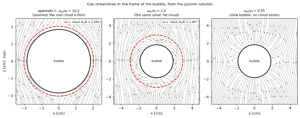
Where the cloud exists, and how big it is
\(V_c/V_b = 3/(u_{br}/u_f - 1)\) has a pole at \(u_{br} = u_f\). The cloud is therefore not a smoothly varying property of the bed: it is unbounded on one side of a threshold and undefined on the other. Marking the paper’s own three appendix beds on that curve:
ratio = np.geomspace(1.02, 60, 400)
vc = 3.0 / (ratio - 1.0)
fig, ax = plt.subplots(1, 2, figsize=(9.6, 3.8))
ax[0].loglog(ratio, vc, "C0-", lw=2)
ax[0].loglog(ratio, (1 + vc) ** (1 / 3), "C1-", lw=2)
ax[0].axvline(1.0, color="0.3", ls=":")
for k, b in BEDS.items():
    x = b["ubr"] / b["uf"]
    if x > 1:
        ax[0].plot(x, 3 / (x - 1), "ko", ms=6)
        ax[0].annotate(k, (x, 3 / (x - 1)), textcoords="offset points", xytext=(6, 4), fontsize=9)
    else:
        ax[0].axvline(x, color="C3", lw=1.5)
        ax[0].annotate(f"{k}: no cloud", (x, 20), rotation=90, color="C3", fontsize=8, ha="right")
ax[0].set_xlabel(r"$u_{br}/u_f = 0.711(gd_b)^{1/2}\,\varepsilon_{mf}/u_{mf}$")
ax[0].set_ylabel("cloud size [-]")
ax[0].legend(["$V_c/V_b$ (eq. 9)", "$R_c/R$"], fontsize=8)
ax[0].set_title("the cloud has a threshold, not a limit", fontsize=9)

db = np.geomspace(0.05, 20, 300)
for k, b in BEDS.items():
    ub = rise_velocity(db)
    v = np.where(ub > b["uf"], 3 * b["uf"] / np.abs(ub - b["uf"]), np.nan)
    ln, = ax[1].loglog(db, v, lw=2, label=f"{k}: $u_f$ = {b['uf']:.2f} cm/s")
    if b["ubr"] > b["uf"]:
        ax[1].plot(b["db"], 3 * b["uf"] / (b["ubr"] - b["uf"]), "o", color=ln.get_color(), ms=7)
b = BEDS["B"]
DB_THR = (b["uf"] / 0.711) ** 2 / G          # u_br(d_b) = u_f: no cloud below this
ax[1].axvline(b["db"], color="C1", ls="--", lw=1.2)
ax[1].annotate(f"B's fitted $d_b$ = {b['db']:.2f} cm\nis below its own\nthreshold {DB_THR:.2f} cm",
               (b["db"], 600.0), textcoords="offset points", xytext=(-5, 0),
               ha="right", va="top", fontsize=7.5, color="C1")
ax[1].set_xlabel("$d_b$ [cm]"); ax[1].set_ylabel("$V_c/V_b$ [-]")
ax[1].set_title("and it is the most $d_b$-sensitive thing in the model", fontsize=9)
ax[1].legend(fontsize=8)
fig.tight_layout(); plt.show()

print("cloud size at the paper's own three appendix beds (closed form)")
print(f"{'':10}{'u_br/u_f':>10}{'V_c/V_b':>12}{'R_c/R':>10}")
for k, b in BEDS.items():
    x = b["ubr"] / b["uf"]
    if x > 1:
        print(f"  {k:8}{x:10.3f}{3 / (x - 1):12.4f}{cloud_radius_exact(b['uf'], b['ubr']):10.4f}")
    else:
        print(f"  {k:8}{x:10.3f}   slow bubble, no cloud; eq. 9 would give V_c/V_b = {3 / (x - 1):.2f}")


def appendix_B_verdict(c_ubr=0.711):
    """Appendix B's cloud threshold, at its stated eps_mf and at the one its printed row implies."""
    b = BEDS["B"]
    ubr = rise_velocity(b["db"], c_ubr)
    emf_implied = 1.0 - printed[("B", "one_minus_ef_times_ub")] / ubr   # (1-eps_mf) u_br = 8.70
    return dict(ubr_over_uf=ubr / b["uf"], vc_eq9=3 / (ubr / b["uf"] - 1),
                db_threshold=(b["uf"] / c_ubr) ** 2 / G, emf_implied=emf_implied,
                ubr_over_uf_implied=ubr * emf_implied / b["umf"], emf_needed=b["umf"] / ubr)


VB = appendix_B_verdict()
print(f"\nappendix B: u_br/u_f = {VB['ubr_over_uf']:.3f}, eq. 9 gives V_c/V_b = {VB['vc_eq9']:.2f}; "
      f"a cloud needs d_b > {VB['db_threshold']:.3f} cm")
print(f"  its printed (1-eps_f)(u_0+5.8) = {printed[('B', 'one_minus_ef_times_ub')]:.2f} implies "
      f"eps_mf = {VB['emf_implied']:.3f} (recorded on E2.1),")
print(f"  which moves u_br/u_f from {VB['ubr_over_uf']:.3f} to {VB['ubr_over_uf_implied']:.3f}: "
      "further below 1, not nearer it.")
print(f"  a cloud would need eps_mf > {VB['emf_needed']:.3f} at this d_b; both values are below.")
for key, name in (("ubr_over_uf", "ubr_over_uf_B"), ("vc_eq9", "Vc_over_Vb_eq9_B"),
                  ("db_threshold", "db_threshold_B"), ("emf_implied", "emf_implied_B"),
                  ("ubr_over_uf_implied", "ubr_over_uf_B_implied"), ("emf_needed", "emf_needed_B")):
    claims.value(name, VB[key], rtol=1e-6, note="closed-form arithmetic on appendix B")
VB_072 = appendix_B_verdict(c_ubr=0.72)
for key, name in (("ubr_over_uf", "ubr_over_uf_B"), ("vc_eq9", "Vc_over_Vb_eq9_B"),
                  ("db_threshold", "db_threshold_B"), ("emf_implied", "emf_implied_B"),
                  ("ubr_over_uf_implied", "ubr_over_uf_B_implied"), ("emf_needed", "emf_needed_B")):
    brk("rise-velocity coefficient 0.72 for 0.711 (c_ubr=0.72)", name, VB_072[key])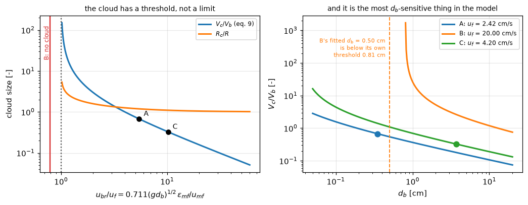
cloud size at the paper's own three appendix beds (closed form)
            u_br/u_f     V_c/V_b     R_c/R
  A            5.441      0.6755    1.1877
  B            0.787   slow bubble, no cloud; eq. 9 would give V_c/V_b = -14.08
  C           10.194      0.3263    1.0987

appendix B: u_br/u_f = 0.787, eq. 9 gives V_c/V_b = -14.08; a cloud needs d_b > 0.807 cm
  its printed (1-eps_f)(u_0+5.8) = 8.70 implies eps_mf = 0.447 (recorded on E2.1),
  which moves u_br/u_f from 0.787 to 0.704: further below 1, not nearer it.
  a cloud would need eps_mf > 0.635 at this d_b; both values are below.
Appendix B of the source paper is on the wrong side of that threshold. Its printed \(d_b\) = 0.50 cm, \(u_{mf}\) = 10 cm/s and \(\varepsilon_{mf}\) = 0.50 give \(u_{br}/u_f\) = 0.787, and equation 9 would give \(V_c/V_b\) = -14.1. Nothing in the paper is wrong: appendix B is a heat-transfer example that needs \(\gamma_b\) and \(H_{bc}\) and never evaluates equation 9. But a reader who carries equation 9 into a bed like that gets a nonsense number with no quantitative warning: the paper says equation 9 is for “beds with fast rising bubbles” and never says how fast is fast. The bubble would have to exceed \(d_b\) = 0.81 cm for a cloud to exist there.
The verdict does not depend on the one appendix-B number in doubt. Its printed \((1-\varepsilon_f)(u_0+5.8)\) implies \(\varepsilon_{mf}\) = 0.447 rather than the stated 0.50. A smaller \(\varepsilon_{mf}\) makes \(u_f = u_{mf}/\varepsilon_{mf}\) larger, so it moves \(u_{br}/u_f\) down to 0.704, further from the threshold, not nearer. Nothing below \(\varepsilon_{mf}\) = 0.635 gives that bed a cloud.
Validation
Route 1: worked examples with printed intermediates. Kunii & Levenspiel print three appendices, and every one of them evaluates one of these single-bubble quantities with the arithmetic shown and the answer stated. Appendix C’s \(\gamma_c\) line is a fully substituted evaluation of equation 9. All of these printed values are already published on E2.1, from the same single transcription this page loads. Recomputing them here checks that the transcription was read the same way twice; it is not independent corroboration, and nobody should count it twice.
Route 2: an internal identity the model must satisfy. The through-flow computed from the numerical field rebuilds the 4.5 that Kunii and Levenspiel print in equations 10 and 11. That coefficient is never an input; it comes out of \(-f'(R) = 3u_f\) and the surface integral. The closed form derived on this page gives the same number, so what the pymrm solve contributes is a check that the discrete operator, with the stated boundary conditions, reproduces the derived field.
Then the numerical machinery is checked against the closed form (which tests the discretisation, not the physics), the far-field condition is measured rather than assumed, and the cloud radius is obtained a second way: by integrating gas trajectories through cubic-spline interpolants of the computed velocity amplitudes, and bisecting on the release radius until a trajectory stops returning to the bubble. What that route confirms is the topology claim, that the zero of \(W\) is where gas stops returning; it uses the same computed field.
Every claim is registered with how it is checked, and the break table at the end injects one defect at a time through an argument of the model and reports which claims catch it.
1. Grid convergence against the closed form
The closed form is \(f = -u_f(r - R^3/r^2)\), \(g = -u_{br}(r + R^3/2r^2)\) and \(R_c/R = [(u_{br} + 2u_f)/(u_{br} - u_f)]^{1/3}\). The ladder is nested (every face of a coarse grid is a face of the finer ones); the observed order of the cloud radius comes from pymrm.checks.observed_orders, which needs no exact solution.
R, uf, ubr = R_C, C["uf"], C["ubr"]
RC_EXACT = R * cloud_radius_exact(uf, ubr)
NS = (100, 200, 400, 800, 1600)
LAD = {n: DavidsonBubble(R, uf, ubr, n=n).solve() for n in NS}


def field_error(s):
    """Largest error of the gas potential at cell centres, relative to u_f R."""
    return np.max(np.abs(s.f - s.f_exact(s.x_c))) / (s.u_f * R)


def coeff_45(s, b=C):
    """(q / V_b) d_b / u_mf: the through-flow coefficient, 4.5 for a sphere."""
    return s.throughflow_per_volume(b["emf"]) * b["db"] / b["umf"]


print(f"   {'n':>6}{'max|f - f_exact|/u_f R':>26}{'|4.5 err|/4.5':>15}{'|R_c err|/R':>14}{'order(f)':>10}")
err_f = []
for n in NS:
    s = LAD[n]
    err_f.append(field_error(s))
    order = "" if len(err_f) < 2 else f"{np.log2(err_f[-2] / err_f[-1]):10.3f}"
    print(f"   {n:6d}{err_f[-1]:26.3e}{abs(coeff_45(s) - 4.5) / 4.5:15.3e}"
          f"{abs(s.cloud_radius() - RC_EXACT) / R:14.3e}{order}")
OO = observed_orders(lambda n: LAD[n].cloud_radius() / R, NS)
FINEST = abs(LAD[NS[-1]].cloud_radius() - LAD[NS[-2]].cloud_radius()) / R
FLOOR = NS[-1] * EPS      # a face gradient divides a cell difference by the cell width
print(f"\n   order of the field error, n = {NS[-2]} to {NS[-1]}:       {np.log2(err_f[-2] / err_f[-1]):.3f}")
print(f"   observed order of R_c (observed_orders, finest triple): {OO['orders'][-1]:.3f}")
print(f"   finest R_c difference / round-off floor n eps:        {FINEST / FLOOR:.1e}")
print(f"   R_c error at n = {N_REF}: {abs(RC_C - RC_EXACT) / R:.1e} of R; field error {err_f[-1]:.1e}")
claims.bound("grid_order_observed", np.log2(err_f[-2] / err_f[-1]), min=1.95, max=2.05,
             basis="theory", note="field error against the closed form, n = 800 to 1600")
claims.bound("Rc_order_observed", OO["orders"][-1], min=1.9, max=2.1, basis="theory",
             note="observed_orders on R_c/R, nested ladder 400, 800, 1600")
claims.bound("grid_finest_over_roundoff", FINEST / FLOOR, min=1e3, basis="theory",
             note="finest R_c difference against n eps")
claims.value("f_field_rel_error_n1600", err_f[-1])
claims.value("Rc_rel_error_n1600", abs(RC_C - RC_EXACT) / R)
_same = {n: LAD[min(n, NS[-2])] for n in NS}
_err_same = [field_error(_same[n]) for n in NS]
_row = f"finest rung solved on n = {NS[-2]} again (refinement not passed)"
brk(_row, "grid_order_observed", np.log2(_err_same[-2] / _err_same[-1]))
_oo_same = observed_orders(lambda n: _same[n].cloud_radius() / R, NS)["orders"][-1]
brk(_row, "Rc_order_observed", _oo_same)   # nan (no convergence) counts as caught
brk(_row, "grid_finest_over_roundoff",
    abs(_same[NS[-1]].cloud_radius() - _same[NS[-2]].cloud_radius()) / R / FLOOR)
n max|f - f_exact|/u_f R |4.5 err|/4.5 |R_c err|/R order(f)
100 5.087e-04 2.986e-04 1.988e-05
200 1.272e-04 7.264e-05 4.789e-06 1.999
400 3.182e-05 1.790e-05 1.174e-06 2.000
800 7.955e-06 4.444e-06 2.906e-07 2.000
1600 1.989e-06 1.107e-06 7.228e-08 2.000
order of the field error, n = 800 to 1600: 2.000
observed order of R_c (observed_orders, finest triple): 2.017
finest R_c difference / round-off floor n eps: 6.1e+05
R_c error at n = 1600: 7.2e-08 of R; field error 2.0e-062. The far-field condition, measured
The Robin condition is exact for the continuous problem, so moving \(r_{out}\) should change the answer only through the discretisation of the cells it adds. The test keeps the cells near the bubble identical: the domain is extended from \(20R\) to \(400R\) by doubling n on the same geometric spacing, so the \(20R\) grid is the first half of the \(400R\) grid. A Dirichlet far field \(h = A r_{out}\), which truncates the decaying mode, is the comparison.
def far_field_shift(far_field, n=N_REF):
    """R_c and the 4.5 coefficient at r_out = 20 R and 400 R, same cells near the bubble."""
    a = DavidsonBubble(R, uf, ubr, n=n, r_out_mult=20.0, far_field=far_field).solve()
    b = DavidsonBubble(R, uf, ubr, n=2 * n, r_out_mult=400.0, far_field=far_field).solve()
    return (abs(a.cloud_radius() - b.cloud_radius()) / R,
            abs(coeff_45(a) - coeff_45(b)) / 4.5, a, b)


FF_RC, FF_Q, _, _ = far_field_shift("robin")
FD_RC, FD_Q, _fd20, _ = far_field_shift("dirichlet")
print(f"   {'far field':>10}{'R_c shift / R':>16}{'4.5 shift / 4.5':>18}")
print(f"   {'Robin':>10}{FF_RC:16.1e}{FF_Q:18.1e}")
print(f"   {'Dirichlet':>10}{FD_RC:16.1e}{FD_Q:18.1e}")
print(f"\n   Robin: R_c moves below 1e-9 of R (here {FF_RC:.1e}); the coefficient moves "
      f"{FF_Q:.1e},")
print("   the same order as its discretisation error at n = 1600 (section 1). Whether that")
print("   shift is discretisation or truncation shows in how it falls when the grid is refined:")
FF_HALF = far_field_shift("robin", N_REF // 2)[1]
FD_HALF = far_field_shift("dirichlet", N_REF // 2)[1]
FF_ORDER = np.log2(FF_HALF / FF_Q)
FD_ORDER = np.log2(FD_HALF / FD_Q)
print(f"   {'n':>6}{'Robin coef shift':>20}{'Dirichlet coef shift':>24}")
print(f"   {N_REF // 2:6d}{FF_HALF:20.2e}{FD_HALF:24.2e}")
print(f"   {N_REF:6d}{FF_Q:20.2e}{FD_Q:24.2e}")
print(f"   order of the fall, n = {N_REF // 2} to {N_REF}: Robin {FF_ORDER:.2f}, Dirichlet {FD_ORDER:.2f}")
print("   The Robin shift falls at the order of the scheme, so it is discretisation; a")
print("   truncation error would not fall with n. The Dirichlet condition at 20 R")
print(f"   puts the cloud {abs(_fd20.cloud_radius() - RC_EXACT) / R:.1e} of R off the closed form.")
claims.bound("far_field_robin_shift_Rc", FF_RC, max=1e-9, basis="theory",
             note="no truncation by the Robin condition; nested extension 20 R to 400 R")
claims.value("far_field_robin_shift_coef", FF_Q,
             note="discretisation error of the added outer cells")
claims.bound("far_field_shift_order", FF_ORDER, min=1.9, max=2.1, basis="theory",
             note="order of the fall of the Robin coefficient shift, n = 800 to 1600")
brk("Dirichlet far field h = A r_out (far_field='dirichlet')", "far_field_shift_order", FD_ORDER)
brk("Dirichlet far field h = A r_out (far_field='dirichlet')", "far_field_robin_shift_Rc", FD_RC)
brk("Dirichlet far field h = A r_out (far_field='dirichlet')", "far_field_robin_shift_coef", FD_Q)
far field R_c shift / R 4.5 shift / 4.5
Robin 9.6e-12 5.8e-07
Dirichlet 1.9e-05 1.3e-04
Robin: R_c moves below 1e-9 of R (here 9.6e-12); the coefficient moves 5.8e-07,
the same order as its discretisation error at n = 1600 (section 1). Whether that
shift is discretisation or truncation shows in how it falls when the grid is refined:
n Robin coef shift Dirichlet coef shift
800 2.33e-06 1.27e-04
1600 5.84e-07 1.26e-04
order of the fall, n = 800 to 1600: Robin 2.00, Dirichlet 0.02
The Robin shift falls at the order of the scheme, so it is discretisation; a
truncation error would not fall with n. The Dirichlet condition at 20 R
puts the cloud 1.9e-05 of R off the closed form.3. The cloud radius a second way: the fate of gas trajectories
def two_routes(n_halvings=45):
    """Relative gap between the trajectory route and the zero of W, appendix C."""
    return abs(cloud_radius_by_trajectories(solC, n_halvings=n_halvings) - RC_C) / RC_C


RC_TRAJ_GAP = two_routes()
print(f"   zero of W (face values, linear in r^-3)        R_c = {RC_C:.9f} cm")
print(f"   bisection on trajectory fate (spline field)    gap below 1e-10 (here {RC_TRAJ_GAP:.1e})")
print(f"   closed form                                    R_c = {RC_EXACT:.9f} cm")
print("   Both read the same computed field; the trajectory route interpolates it with cubic")
print("   splines and bisects 45 times. W = 0 is invariant under the trajectory ODE, so the gap")
print("   is the difference between the two interpolants of the same face values.")
claims.bound("Rc_two_routes_rel", RC_TRAJ_GAP, max=1e-10, basis="tolerance",
             note="45 bisection halvings; cubic spline against linear-in-r^-(nu+1) interpolant")
brk("trajectory bisection stopped after 20 halvings (n_halvings=20)", "Rc_two_routes_rel",
    two_routes(20))
zero of W (face values, linear in r^-3) R_c = 2.032606036 cm
bisection on trajectory fate (spline field) gap below 1e-10 (here 2.4e-12)
closed form R_c = 2.032606170 cm
Both read the same computed field; the trajectory route interpolates it with cubic
splines and bisects 45 times. W = 0 is invariant under the trajectory ODE, so the gap
is the difference between the two interpolants of the same face values.4. The through-flow rebuilds the 4.5 that opens equations 10 and 11
\(q = \varepsilon_{mf}(-f'(R))\,\pi R^2\) is the outflow over the upper hemisphere, and \(q/V_b\) with \(V_b = \tfrac43\pi R^3\). With \(-f'(R) = 3u_f\) this is \(4.5\,u_{mf}/d_b\): \(\varepsilon_{mf}\), \(u_{mf}\) and \(d_b\) cancel, so the coefficient is a pure number, and on a grid geometric in \(r/R\) even its discretisation error is the same for the three beds. They are not three confirmations. The check does not require a fast bubble: \(u_{br}\) never enters the gas potential.
print(f"   {'bed':>5}{'q/V_b [1/s]':>14}{'(q/V_b) d_b/u_mf':>20}{'printed':>10}{'dev':>10}")
SOL = {"C": solC}
for k, b in BEDS.items():
    SOL.setdefault(k, DavidsonBubble(b["db"] / 2, b["uf"], b["ubr"], n=N_REF).solve())
    b["q_over_Vb"] = SOL[k].throughflow_per_volume(b["emf"])
    cf = coeff_45(SOL[k], b)
    print(f"   {k:>5}{b['q_over_Vb']:14.5f}{cf:20.6f}{4.5:10.1f}{abs(cf - 4.5) / 4.5:10.2e}")
COEF_ERR = max(abs(coeff_45(SOL[k], b) - 4.5) / 4.5 for k, b in BEDS.items())
print(f"\n   worst over the three beds: {COEF_ERR:.1e}, the discretisation error at n = {N_REF}")
claims.value("throughflow_coefficient_rel", COEF_ERR,
             note="|coefficient - 4.5| / 4.5, worst of the three beds, n = 1600")
bed q/V_b [1/s] (q/V_b) d_b/u_mf printed dev
A 15.55713 4.499995 4.5 1.11e-06
B 89.99990 4.499995 4.5 1.11e-06
C 2.55405 4.499995 4.5 1.11e-06
worst over the three beds: 1.1e-06, the discretisation error at n = 16005. K_bc, H_bc and the printed appendix values, recomputed
\(K_{bc}\) and \(H_{bc}\) are reassembled from the derived through-flow plus the printed 5.85 diffusive terms, and compared with the appendices’ printed totals. The printed single-bubble values are recomputed from equations 3 and 17, with \(\gamma_c\) evaluated twice: with equation 9 as printed, and with the cloud from the pymrm solve.
def rebuilt_K_H(q):
    """K_bc (appendices A, C) and H_bc (appendix B) from through-flows q[k] [1/s]."""
    A, B = BEDS["A"], BEDS["B"]
    return [("K_bc, appendix A [1/s]", q["A"] + 5.85 * A["D"] ** 0.5 * G ** 0.25 / A["db"] ** 1.25,
             printed[("A", "K_bc")]),
            ("K_bc, appendix C [1/s]", q["C"] + 5.85 * C["D"] ** 0.5 * G ** 0.25 / C["db"] ** 1.25,
             printed[("C", "K_bc")]),
            ("H_bc, appendix B [cal/cc s C]", q["B"] * B["rho_g"] * B["Cpg"]
             + 5.85 * (B["kg"] * B["rho_g"] * B["Cpg"]) ** 0.5 * G ** 0.25 / B["db"] ** 1.25,
             printed[("B", "H_bc")])]


def worst_pct(rows):
    return max(100 * abs(got - want) / want for _, got, want in rows)


def gamma_c(Rc_over_R):
    """Equation 17 with V_c/V_b = (R_c/R)^3 - 1."""
    return (1 - C["emf"]) * (Rc_over_R ** 3 - 1 + C["alpha"])


def appendix_rows(c_ubr=0.711, Rc_over_R=RC_C / R_C):
    A, B = BEDS["A"], BEDS["B"]
    ubr = {k: rise_velocity(b["db"], c_ubr) for k, b in BEDS.items()}
    gc_eq9 = (1 - C["emf"]) * (3 * C["uf"] / (ubr["C"] - C["uf"]) + C["alpha"])   # eq. 17 verbatim
    return [("u_b - u_0, appendix A [cm/s]", ubr["A"] - A["umf"], printed[("A", "ub_minus_u0")]),
            ("u_b - u_0, appendix B [cm/s]", ubr["B"] - B["umf"], printed[("B", "ub_minus_u0")]),
            ("u_br, appendix C [cm/s]", ubr["C"], printed[("C", "u_br")]),
            ("u_b, appendix C [cm/s]", C["u0"] - C["umf"] + ubr["C"], printed[("C", "u_b")]),
            ("gamma_c, appendix C (eq. 9 as printed)", gc_eq9, printed[("C", "gamma_c")]),
            ("gamma_c, appendix C (cloud from pymrm)", gamma_c(Rc_over_R), printed[("C", "gamma_c")])]


Q = {k: b["q_over_Vb"] for k, b in BEDS.items()}
KH, APP = rebuilt_K_H(Q), appendix_rows()
print(f"   {'quantity':>40}{'computed':>12}{'printed':>10}{'dev':>9}")
for name, got, want in KH + APP:
    print(f"   {name:>40}{got:12.5g}{want:10.5g}{100 * abs(got - want) / want:8.2f} %")
GC_EQ9, GC_NUM = APP[4][1], APP[5][1]
u0_from_csv = printed[("C", "u_b")] - printed[("C", "u_br")] + C["umf"]
print(f"\n   appendix C's u_0 from the CSV's printed u_b and u_br: {u0_from_csv:.1f} cm/s "
      f"(the value used: {C['u0']:.1f} cm/s)")
print(f"   gamma_c from the pymrm cloud against eq. 9 as printed: {abs(GC_NUM - GC_EQ9) / GC_EQ9:.1e} relative")
claims.value("Kbc_Hbc_worst_pct", worst_pct(KH), unit="%")
claims.value("appendix_worst_pct", worst_pct(APP), unit="%")
claims.value("gamma_c_from_pymrm_cloud_pct", 100 * abs(GC_NUM - printed[("C", "gamma_c")])
             / printed[("C", "gamma_c")], unit="%")
claims.value("gamma_c_pymrm_vs_eq9", abs(GC_NUM - GC_EQ9) / GC_EQ9,
             note="discretisation error of the cloud radius, carried into eq. 17")
quantity computed printed dev
K_bc, appendix A [1/s] 46.555 46.5 0.12 %
K_bc, appendix C [1/s] 5.4349 5.44 0.09 %
H_bc, appendix B [cal/cc s C] 0.035845 0.036 0.43 %
u_b - u_0, appendix A [cm/s] 11.958 12 0.35 %
u_b - u_0, appendix B [cm/s] 5.7387 5.8 1.06 %
u_br, appendix C [cm/s] 42.814 42.8 0.03 %
u_b, appendix C [cm/s] 53.914 53.9 0.03 %
gamma_c, appendix C (eq. 9 as printed) 0.39815 0.4 0.46 %
gamma_c, appendix C (cloud from pymrm) 0.39815 0.4 0.46 %
appendix C's u_0 from the CSV's printed u_b and u_br: 13.2 cm/s (the value used: 13.2 cm/s)
gamma_c from the pymrm cloud against eq. 9 as printed: 3.3e-07 relative6. The limits the model must have
Seven values of \(u_{br}/u_f\) from 1.001 to 1000, so \(u_{br}/u_f - 1\) spans six decades. At 1.001 the cloud sits at \(14.4R\), inside the \(20R\) domain; closer to the threshold it moves outside, and the model then raises instead of reporting no cloud.
X_LIM = (1.001, 1.01, 1.1, 2.0, 10.0, 100.0, 1000.0)


def limits(**kw):
    """Worst relative deviation of R_c/R from the closed form over X_LIM."""
    rows = []
    for x in X_LIM:
        rc = DavidsonBubble(1.0, 1.0, x, n=N_REF, **kw).solve().cloud_radius()
        rows.append((x, rc, cloud_radius_exact(1.0, x)))
    return rows, max(abs(rc - ex) / ex for _, rc, ex in rows)


LIM, LIM_WORST = limits()
print(f"   {'u_br/u_f':>10}{'R_c/R numeric':>16}{'closed form':>14}")
for x, rc, ex in LIM:
    print(f"   {x:10.3f}{rc:16.6f}{ex:14.6f}")
print(f"\n   u_br/u_f - 1 spans {np.log10((X_LIM[-1] - 1) / (X_LIM[0] - 1)):.0f} decades; "
      f"worst deviation {LIM_WORST:.1e}")
slow_rc = DavidsonBubble(1.0, 1.0, 0.9, n=N_REF).solve().cloud_radius()
print(f"   u_br/u_f = 0.90: the model returns {slow_rc} (no zero of W, and u_br < u_f: no cloud)")
try:
    DavidsonBubble(1.0, 1.0, 1.0001, n=N_REF).solve().cloud_radius()
except RuntimeError as e:
    print(f"   u_br/u_f = 1.0001: raises, '{e}'")
claims.value("limit_worst_rel", LIM_WORST)
claims.value("Rc_over_R_x1001", LIM[0][1], rtol=1e-4, note="R_c/R at u_br/u_f = 1.001")
_lim_d = limits(far_field="dirichlet")
brk("Dirichlet far field h = A r_out (far_field='dirichlet')", "limit_worst_rel", _lim_d[1])
brk("Dirichlet far field h = A r_out (far_field='dirichlet')", "Rc_over_R_x1001", _lim_d[0][0][1])
u_br/u_f R_c/R numeric closed form
1.001 14.424090 14.424098
1.010 6.701756 6.701759
1.100 3.141380 3.141381
2.000 1.587401 1.587401
10.000 1.100642 1.100642
100.000 1.010001 1.010001
1000.000 1.001000 1.001000
u_br/u_f - 1 spans 6 decades; worst deviation 5.3e-07
u_br/u_f = 0.90: the model returns nan (no zero of W, and u_br < u_f: no cloud)
u_br/u_f = 1.0001: raises, 'no zero of W inside r_out although u_br > u_f: the cloud lies beyond r_out, enlarge the domain'7. The discrete integral identity, and what it can see
Integrating the radial equation once over \([R, r_{out}]\) gives \(\int_R^{r_{out}} \nu h\, r^{\nu-2}\,dr = [r^\nu h']_R^{r_{out}}\). On the discrete solution, the gap is the volume-weighted sum of the discrete residuals, which telescopes for any consistent (construct_div, cell volume, \(\nu\)) triple with any boundary data. It is not a check on the physics. What it can see is a mismatch between the geometry index inside construct_div and the coefficient of the sink term.
def identity(s):
    return max(s.integral_identity("gas"), s.integral_identity("solids"))


ID_GAP = identity(solC)
print(f"   both potentials, appendix C: below 1e-10 (here {ID_GAP:.1e})")
claims.bound("integral_identity_gap", ID_GAP, max=1e-10, basis="identity",
             note="telescoping sum; detects a nu mismatch between construct_div and the sink")
both potentials, appendix C: below 1e-10 (here 2.0e-12)8. The two-dimensional bubble: the same operator with nu=1
def bubble_2d(**kw):
    return DavidsonBubble(R_C, C["uf"], C["ubr"], n=N_REF, nu=1, **kw).solve()


def results_2d(s):
    rc = s.cloud_radius() / R_C
    ex = cloud_radius_exact(C["uf"], C["ubr"], nu=1)
    return rc, abs(rc - ex) / ex, s.throughflow_per_volume(C["emf"]) * C["db"] / C["umf"]


RC2, RC2_ERR, Q2 = results_2d(bubble_2d())
print(f"   R_c/R = {RC2:.6f} against the 3-D {RC_C / R_C:.6f}")
print(f"   closed form [(u_br+u_f)/(u_br-u_f)]^(1/2): deviation {RC2_ERR:.1e}")
print(f"   through-flow per unit bubble area: {Q2:.6f} u_mf/d_b, closed form 8/pi = {8 / np.pi:.6f}")
claims.value("Rc2_over_R_C", RC2, rtol=1e-6)
claims.value("cloud_2d_rel_error", RC2_ERR)
claims.value("throughflow_2d_coefficient", Q2, rtol=1e-4,
             note="closed form 8/pi; discretisation error about 1e-6")
_b2 = results_2d(bubble_2d(sink_coeff=2))
for name, v in zip(("Rc2_over_R_C", "cloud_2d_rel_error", "throughflow_2d_coefficient"), _b2):
    brk("2-D model with the 3-D sink coefficient (nu=1, sink_coeff=2)", name, v)
R_c/R = 1.103421 against the 3-D 1.098706
closed form [(u_br+u_f)/(u_br-u_f)]^(1/2): deviation 3.9e-08
through-flow per unit bubble area: 2.546478 u_mf/d_b, closed form 8/pi = 2.5464799. Break it on purpose
Each row re-solves appendix C’s bubble (or the case of its claim) with exactly one thing injected through an argument of DavidsonBubble, and records what every claim it should move becomes. The table is computed when the cell runs.
DEFECTS = [
    ("far-field factor nu for nu + 1 (far_factor=2)", dict(far_factor=2.0)),
    ("geometry index 1 in construct_div only (nu_div=1)", dict(nu_div=1)),
    ("sink coefficient 1 (sink_coeff=1)", dict(sink_coeff=1)),
    ("sink coefficient 6, the l = 2 harmonic (sink_coeff=6)", dict(sink_coeff=6)),
    ("2-D operator in the 3-D model (nu_div=1, sink_coeff=1)", dict(nu_div=1, sink_coeff=1)),
    ("outer bc a = -1, outward normal flipped (outer_a=-1)", dict(outer_a=-1.0)),
    ("outer bc datum sign flipped (outer_d_sign=-1)", dict(outer_d_sign=-1.0)),
    ("Dirichlet far field h = A r_out (far_field='dirichlet')", dict(far_field="dirichlet")),
]
print(f"   {'injected defect':<56}{'4.5 ->':>9}{'field err':>11}{'R_c/R err':>11}{'identity':>11}")
DEF = {}
for name, kw in DEFECTS:
    sd = DavidsonBubble(R, uf, ubr, n=N_REF, **kw).solve()
    rc = sd.cloud_radius()
    DEF[name] = (sd, rc)
    print(f"   {name:<56}{coeff_45(sd):9.3f}{field_error(sd):11.1e}"
          f"{abs(rc - RC_EXACT) / R:11.1e}{identity(sd):11.1e}")
    others = {}
    for k, b in BEDS.items():
        others[k] = (sd if k == "C" else
                     DavidsonBubble(b["db"] / 2, b["uf"], b["ubr"], n=N_REF, **kw).solve())
    brk(name, "throughflow_coefficient_rel",
        max(abs(coeff_45(others[k], b) - 4.5) / 4.5 for k, b in BEDS.items()))

_mismatch = [n for n, kw in DEFECTS if "nu_div" in kw or "sink_coeff" in kw]   # differ from nu = 2
_blind = [n for n in DEF if n not in _mismatch]
for name in _mismatch:
    brk(name, "integral_identity_gap", identity(DEF[name][0]))
BLIND = max(identity(DEF[n][0]) for n in _blind)
claims.bound("defect_identity_worst_blind", BLIND, max=1e-10, basis="identity", structural=True,
             note="consistent defects: the identity telescopes whatever the nu and the bc")

_far2 = "far-field factor nu for nu + 1 (far_factor=2)"
brk(_far2, "f_field_rel_error_n1600", field_error(DEF[_far2][0]))
brk(_far2, "Kbc_Hbc_worst_pct", worst_pct(rebuilt_K_H(
    {k: DavidsonBubble(b["db"] / 2, b["uf"], b["ubr"], n=N_REF, far_factor=2.0).solve()
     .throughflow_per_volume(b["emf"]) for k, b in BEDS.items()})))
_dirich = "Dirichlet far field h = A r_out (far_field='dirichlet')"
brk(_dirich, "Rc_rel_error_n1600", abs(DEF[_dirich][1] - RC_EXACT) / R)
_op2d = "2-D operator in the 3-D model (nu_div=1, sink_coeff=1)"
_rc2d = DEF[_op2d][1] / R
brk(_op2d, "Rc_over_R_C", _rc2d)
brk(_op2d, "cloud_shell_C", _rc2d - 1)
_app2d = appendix_rows(Rc_over_R=_rc2d)
brk(_op2d, "gamma_c_from_pymrm_cloud_pct",
    100 * abs(_app2d[5][1] - printed[("C", "gamma_c")]) / printed[("C", "gamma_c")])
brk(_op2d, "gamma_c_pymrm_vs_eq9", abs(_app2d[5][1] - _app2d[4][1]) / _app2d[4][1])
brk("rise-velocity coefficient 0.72 for 0.711 (c_ubr=0.72)", "appendix_worst_pct",
    worst_pct(appendix_rows(c_ubr=0.72)))

print(f"\n   the identity, on the {len(_blind)} consistent defects: below 1e-10 (here {BLIND:.1e}),")
print(f"   on the {len(_mismatch)} nu mismatches: at least {min(identity(DEF[n][0]) for n in _mismatch):.1e}")
_caught45 = sum(c for r, m, _, _, c in BREAK if m == "throughflow_coefficient_rel")
print(f"   the through-flow coefficient fails its check on {_caught45} of {len(DEFECTS)} defects")
_rc_blind = [n for n in DEF if abs(DEF[n][1] - RC_EXACT) / R < 2 * abs(RC_C - RC_EXACT) / R]
print(f"   R_c/R stays at its discretisation error on {len(_rc_blind)}: " + "; ".join(_rc_blind))
injected defect 4.5 -> field err R_c/R err identity
far-field factor nu for nu + 1 (far_factor=2) 3.000 6.7e+00 7.2e-08 2.0e-12
geometry index 1 in construct_div only (nu_div=1) 1.078 3.5e+00 2.7e-02 4.2e-01
sink coefficient 1 (sink_coeff=1) 12.071 4.9e+00 6.1e-02 1.0e+00
sink coefficient 6, the l = 2 harmonic (sink_coeff=6) 0.281 6.7e+00 4.9e-02 6.7e-01
2-D operator in the 3-D model (nu_div=1, sink_coeff=1) 3.003 2.5e-01 4.9e-03 1.5e-02
outer bc a = -1, outward normal flipped (outer_a=-1) 13.507 4.0e+01 7.5e-05 2.0e-12
outer bc datum sign flipped (outer_d_sign=-1) -4.500 4.0e+01 7.2e-08 2.0e-12
Dirichlet far field h = A r_out (far_field='dirichlet') 4.501 2.5e-03 1.9e-05 1.5e-12
the identity, on the 4 consistent defects: below 1e-10 (here 2.0e-12),
on the 4 nu mismatches: at least 1.5e-02
the through-flow coefficient fails its check on 8 of 8 defects
R_c/R stays at its discretisation error on 2: far-field factor nu for nu + 1 (far_factor=2); outer bc datum sign flipped (outer_d_sign=-1)Which line to watch. The discrete integral identity sits at round-off under every consistent defect, including a mis-signed outer boundary condition that ruins the field, and \(R_c/R\) is blind to the two far-field defects that rescale both potentials together, because the zero of \(W = g' - f'\) does not move. The through-flow coefficient, which needs no closed form (it is compared with the printed 4.5), fails its check on every defect in the table; so does the field error, which needs the closed form. If you copy this skeleton, watch the through-flow, not the conservation line.
The break table
print(f"{'injected defect':<64} {'claim':<30} {'clean':>11} {'broken':>11}  caught")
for row, metric, clean, broken, caught in BREAK:
    if claims.metrics[metric]["kind"] == "bound":
        shown, br = f"(here {clean:.3g})", f"{float(broken):.3g}"
    else:
        shown, br = f"{float(clean):11.5g}", f"{float(broken):11.5g}"
    print(f"{row[:64]:<64} {metric[:30]:<30} {shown:>11} {br:>11}  {'yes' if caught else 'NO'}")
_caught = {mt for _, mt, _, _, c in BREAK if c}
_open = sorted(k for k in claims.metrics if k not in _caught and not claims.metrics[k].get("structural"))
print(f"\n{len(BREAK)} rows; {len(_caught)} of {len(claims.metrics)} claims are failed by at least one row; "
      f"open: {', '.join(_open) or 'none'}")
print("rows that do not fail their claim: "
      + ("; ".join(f"{r} -> {mt}" for r, mt, _, _, c in BREAK if not c) or "none"))
injected defect claim clean broken caught
rise-velocity coefficient 0.72 for 0.711 (c_ubr=0.72) ubr_over_uf_B 0.78693 0.79689 yes
rise-velocity coefficient 0.72 for 0.711 (c_ubr=0.72) Vc_over_Vb_eq9_B -14.08 -14.771 yes
rise-velocity coefficient 0.72 for 0.711 (c_ubr=0.72) db_threshold_B 0.80741 0.78735 yes
rise-velocity coefficient 0.72 for 0.711 (c_ubr=0.72) emf_implied_B 0.44722 0.45413 yes
rise-velocity coefficient 0.72 for 0.711 (c_ubr=0.72) ubr_over_uf_B_implied 0.70387 0.72379 yes
rise-velocity coefficient 0.72 for 0.711 (c_ubr=0.72) emf_needed_B 0.63538 0.62744 yes
finest rung solved on n = 800 again (refinement not passed) grid_order_observed (here 2) 0 yes
finest rung solved on n = 800 again (refinement not passed) Rc_order_observed (here 2.02) nan yes
finest rung solved on n = 800 again (refinement not passed) grid_finest_over_roundoff (here 6.15e+05) 0 yes
Dirichlet far field h = A r_out (far_field='dirichlet') far_field_shift_order (here 2) 0.02 yes
Dirichlet far field h = A r_out (far_field='dirichlet') far_field_robin_shift_Rc (here 9.57e-12) 1.87e-05 yes
Dirichlet far field h = A r_out (far_field='dirichlet') far_field_robin_shift_coef 5.835e-07 0.00012558 yes
trajectory bisection stopped after 20 halvings (n_halvings=20) Rc_two_routes_rel (here 2.44e-12) 6.81e-07 yes
Dirichlet far field h = A r_out (far_field='dirichlet') limit_worst_rel 5.3232e-07 0.071719 yes
Dirichlet far field h = A r_out (far_field='dirichlet') Rc_over_R_x1001 14.424 15.459 yes
2-D model with the 3-D sink coefficient (nu=1, sink_coeff=2) Rc2_over_R_C 1.1034 1.0721 yes
2-D model with the 3-D sink coefficient (nu=1, sink_coeff=2) cloud_2d_rel_error 3.8985e-08 0.028419 yes
2-D model with the 3-D sink coefficient (nu=1, sink_coeff=2) throughflow_2d_coefficient 2.5465 0.86256 yes
far-field factor nu for nu + 1 (far_factor=2) throughflow_coefficient_rel 1.1068e-06 0.33333 yes
geometry index 1 in construct_div only (nu_div=1) throughflow_coefficient_rel 1.1068e-06 0.76047 yes
sink coefficient 1 (sink_coeff=1) throughflow_coefficient_rel 1.1068e-06 1.6825 yes
sink coefficient 6, the l = 2 harmonic (sink_coeff=6) throughflow_coefficient_rel 1.1068e-06 0.9375 yes
2-D operator in the 3-D model (nu_div=1, sink_coeff=1) throughflow_coefficient_rel 1.1068e-06 0.33278 yes
outer bc a = -1, outward normal flipped (outer_a=-1) throughflow_coefficient_rel 1.1068e-06 2.0015 yes
outer bc datum sign flipped (outer_d_sign=-1) throughflow_coefficient_rel 1.1068e-06 2 yes
Dirichlet far field h = A r_out (far_field='dirichlet') throughflow_coefficient_rel 1.1068e-06 0.00012397 yes
geometry index 1 in construct_div only (nu_div=1) integral_identity_gap (here 1.96e-12) 0.416 yes
sink coefficient 1 (sink_coeff=1) integral_identity_gap (here 1.96e-12) 1 yes
sink coefficient 6, the l = 2 harmonic (sink_coeff=6) integral_identity_gap (here 1.96e-12) 0.667 yes
2-D operator in the 3-D model (nu_div=1, sink_coeff=1) integral_identity_gap (here 1.96e-12) 0.015 yes
far-field factor nu for nu + 1 (far_factor=2) f_field_rel_error_n1600 1.9888e-06 6.6596 yes
far-field factor nu for nu + 1 (far_factor=2) Kbc_Hbc_worst_pct 0.43047 24.03 yes
Dirichlet far field h = A r_out (far_field='dirichlet') Rc_rel_error_n1600 7.2282e-08 1.8662e-05 yes
2-D operator in the 3-D model (nu_div=1, sink_coeff=1) Rc_over_R_C 1.0987 1.1036 yes
2-D operator in the 3-D model (nu_div=1, sink_coeff=1) cloud_shell_C 0.098706 0.1036 yes
2-D operator in the 3-D model (nu_div=1, sink_coeff=1) gamma_c_from_pymrm_cloud_pct 0.46148 1.7654 yes
2-D operator in the 3-D model (nu_div=1, sink_coeff=1) gamma_c_pymrm_vs_eq9 3.2873e-07 0.022371 yes
rise-velocity coefficient 0.72 for 0.711 (c_ubr=0.72) appendix_worst_pct 1.0577 2.3772 yes
38 rows; 28 of 29 claims are failed by at least one row; open: none
rows that do not fail their claim: noneWhat pymrm adds
Nothing to the closed form. The classical solution is exact and the algebra is short, and every number the solve gives is also given by the closed form derived on this page.
One flow field, read twice. In the reactor literature the cloud volume and the interchange coefficient are two consecutive equations, 9 and 10, and nothing in the paper connects them. Neither is derived; both are stated, with different-looking constants (3 in equation 9, 4.5 in equations 10 and 11). The derivation on this page connects them: \(-f'(R) = 3u_f\) gives the through-flow, and the sum of that gas flux with the solids potential flow gives the dividing streamline. What the pymrm solve adds beyond the derivation is a check of it: the discrete operator, given only the boundary-value problem, reproduces the cloud radius to 7.2e-8 of \(R\) and the 4.5 to 1.1e-6, both at the discretisation error and second order, and the break table shows which output catches which operator error.
A threshold, not a limit. \(V_c/V_b = 3/(u_{br}/u_f - 1)\) has a pole. Below it there is no cloud at all, and equation 9 returns a negative number; applied to the paper’s own appendix beds, this puts appendix B on the wrong side (Results).
The through-flow, unlike the cloud, has no such threshold. \(u_{br}\) never enters the gas potential; the bubble’s speed affects where the gas goes, not how much crosses the surface. So the 4.5 term in equations 10 and 11 holds on both sides of the threshold, and the 3 in equation 9 does not. The two constants are usually quoted together as though they had the same standing. One qualification: what is speed-independent is the volumetric through-flow \(q = 3u_{mf}\pi R^2\). Whether \(q/V_b\) still deserves the name “bubble-to-cloud interchange” below the threshold is an interpretive step, since the series bubble, cloud, emulsion has lost its middle term there.
The two-dimensional bubble, from one argument. nu=1 instead of nu=2 turns the same operator into the slab-bed problem and gives \(R_c/R = [(u_{br}+u_f)/(u_{br}-u_f)]^{1/2}\), an exponent of \(1/2\) instead of \(1/3\), so a larger cloud at the same velocity ratio (1.103 against 1.099 for appendix C’s bed), and a through-flow of \(8u_{mf}/(\pi d_b)\) = 2.55 \(u_{mf}/d_b\) against 4.5 in three dimensions. Photographs of bubbles and clouds mostly come from two-dimensional beds, while the correlations they calibrate are three-dimensional. Kunii & Levenspiel print only the three-dimensional form.
And the honest negative. This page cannot say whether any of it is true. Nothing on it is compared with a measurement (the source contains none for a single bubble), so every number is either the authors’ own arithmetic or this page’s own derivation. Tier 6.
Reuse
from model import DavidsonBubble

s = DavidsonBubble(R=1.85, u_f=4.2, u_br=42.81, n=1600).solve()   # 3-D bubble
s.cloud_radius() / s.R                                             # cloud radius ratio
s.throughflow_per_volume(eps_mf=0.5)                               # q / V_b [1/s]
DavidsonBubble(R=1.85, u_f=4.2, u_br=42.81, nu=1).solve()          # 2-D (slab-bed) bubble
What transfers. DavidsonBubble is not really about bubbles. Its operator is the radial factor of any \(\ell = 1\) spherical or cylindrical harmonic with a mixed set of boundary conditions, which is the shape of every “uniform far field meets a sphere” problem: flow past a drop, a conducting sphere in a uniform electric field, a spherical inclusion in a temperature gradient. The two conditions used here, potential fixed on the sphere and normal derivative zero on the sphere, are the two limiting cases those problems interpolate between.
The exact far-field Robin condition \(h' + (\nu/r)h = (\nu+1)A\) is the reusable trick. Whenever a solution is a sum of a growing and a decaying separable mode, there is a combination of value and derivative that annihilates the decaying one, and imposing it lets a finite domain carry an infinite one with no truncation error; the measurement in the validation shows what is left, the discretisation of the outer cells.
What does not transfer. \(d_b\) is not a measured bubble diameter; in the reactor model it is a fitted effective size, and E2.1 says so at length. The wake fraction \(\alpha\) in equation 17 is empirical and is not part of this theory: potential flow past a sphere has no wake. And the spherical bubble is a convenience: real bubbles are spherical caps.
Where else this structure appears. As a 1D steady BVP with construct_grad, construct_div and a geometry index it is the same S3 skeleton as B1.1 (Thiele modulus), B1.6 (Prater relation) and J1.5 (LDF), differing only in what multiplies the unknown. As physics the continuation is E2.1, which takes \(u_{br}\), \(V_c/V_b\) and \(K_{bc}\) as inputs and builds the bubbling-bed reactor model on them; E1.1 (two-phase theory) is the earlier picture this refines.
And if you copy this skeleton, watch the right line. The number that catches a broken operator here is the through-flow 4.5, not the conservation line. A boundary-sign error is the kind of mistake the identity is built to catch; a closing conservation check is not evidence against one.
# Numbers stated in the Markdown cells, each checked against its claim.
PROSE = [("10 %", "cloud_shell_C"), ("1.099", "Rc_over_R_C"), ("0.787", "ubr_over_uf_B"),
         ("-14.1", "Vc_over_Vb_eq9_B"), ("0.81", "db_threshold_B"), ("0.447", "emf_implied_B"),
         ("0.704", "ubr_over_uf_B_implied"), ("0.635", "emf_needed_B"),
         ("7.2e-8", "Rc_rel_error_n1600"), ("1.1e-6", "throughflow_coefficient_rel"),
         ("1.103", "Rc2_over_R_C"), ("2.55", "throughflow_2d_coefficient"),
         ("14.4", "Rc_over_R_x1001")]
for _lit, _name in PROSE:
    claims.says(_lit, _name)
print(f"{len(PROSE)} prose literals checked against {len({n for _, n in PROSE})} claims")
13 prose literals checked against 13 claims# Claims: prints every registered number, writes agreement.json for CI, and
# raises when a claim fails its own check or has no break row.
claims.report(); # the semicolon keeps the notebook from echoing the payloadClaims for E1.2:
Rc_over_R_C = 1.0987 value rtol 1e-06
cloud_shell_C = 0.098706 value rtol 1e-06
ubr_over_uf_B = 0.78693 value rtol 1e-06
Vc_over_Vb_eq9_B = -14.08 value rtol 1e-06
db_threshold_B = 0.80741 value rtol 1e-06
emf_implied_B = 0.44722 value rtol 1e-06
ubr_over_uf_B_implied = 0.70387 value rtol 1e-06
emf_needed_B = 0.63538 value rtol 1e-06
grid_order_observed = (here 2.0e+00) bound bound [1.95, 2.05] [theory]
Rc_order_observed = (here 2.0e+00) bound bound [1.9, 2.1] [theory]
grid_finest_over_roundoff = (here 6.1e+05) bound bound >= 1000 [theory]
f_field_rel_error_n1600 = 1.9888e-06 value rtol 0.05
Rc_rel_error_n1600 = 7.2282e-08 value rtol 0.05
far_field_robin_shift_Rc = (here 9.6e-12) bound bound <= 1e-09 [theory]
far_field_robin_shift_coef = 5.835e-07 value rtol 0.05
far_field_shift_order = (here 2.0e+00) bound bound [1.9, 2.1] [theory]
Rc_two_routes_rel = (here 2.4e-12) bound bound <= 1e-10 [tolerance]
throughflow_coefficient_rel = 1.1068e-06 value rtol 0.05
Kbc_Hbc_worst_pct = 0.43047 value rtol 0.05
appendix_worst_pct = 1.0577 value rtol 0.05
gamma_c_from_pymrm_cloud_pct = 0.46148 value rtol 0.05
gamma_c_pymrm_vs_eq9 = 3.2873e-07 value rtol 0.05
limit_worst_rel = 5.3232e-07 value rtol 0.05
Rc_over_R_x1001 = 14.424 value rtol 0.0001
integral_identity_gap = (here 2.0e-12) bound bound <= 1e-10 [identity]
Rc2_over_R_C = 1.1034 value rtol 1e-06
cloud_2d_rel_error = 3.8985e-08 value rtol 0.05
throughflow_2d_coefficient = 2.5465 value rtol 0.0001
defect_identity_worst_blind = (here 2.0e-12) bound bound <= 1e-10 [identity]