# Bootstrap: the pymrm this page was checked with, and the gallery files it was
# published with. Works in a checkout, in CI and on a fresh Colab VM.
GALLERY_REF = "gallery-2026.11.10.3"  # replaced by the release tag at publication
PYMRM = ">=3.3.0,<4"  # equals meta.yaml pymrm_min_version, up to the next major
PAGE = "D2.1-barkelew-runaway-diagram"  # equals the page directory

import os, sys, urllib.request
from pathlib import Path
_shared = next((p / "shared" for p in (Path.cwd(), *Path.cwd().parents)
                if (p / "shared" / "gallery_bootstrap.py").is_file()), None)
if _shared is None:
    _shared = (Path(os.environ.get("XDG_CACHE_HOME") or Path.home() / ".cache")
               / "pymrm-gallery" / GALLERY_REF)
    _shared.mkdir(parents=True, exist_ok=True)
    urllib.request.urlretrieve(
        "https://raw.githubusercontent.com/computational-chemical-engineering/"
        f"pymrm-gallery/{GALLERY_REF}/shared/gallery_bootstrap.py",
        _shared / "gallery_bootstrap.py")
sys.path.insert(0, str(_shared))
sys.modules.pop("gallery_bootstrap", None)
from gallery_bootstrap import setup
setup(PAGE, PYMRM, GALLERY_REF); # the semicolon stops the cell echoing the pathBarkelew’s runaway diagram
sec:D
struct:S2
tier:T0
data:tier6
phase:gas-solid
The 1959 chart that collapses the runaway boundary of a cooled tubular reactor onto two dimensionless groups - rebuilt from the paper that reprints it, and tested where a similarity reduction is supposed to fail.
Barkelew’s runaway diagram
Catalog ID: D2.1 · Structures: S2 (plug flow with reaction) · Tier: T0
A cooled tubular reactor runs away when the heat it makes outruns the heat the wall can take. Barkelew integrated that problem a great many times and found that the boundary between safe and unsafe operation collapses onto two dimensionless groups, so that one chart covers every first-order exothermic reaction. This page rebuilds the chart, and then asks the question a collapse always invites: how well does it actually collapse?
from dataclasses import replace
from functools import lru_cache

import numpy as np
import pandas as pd
import matplotlib.pyplot as plt
from IPython.display import Markdown, display
from scipy.interpolate import PchipInterpolator
from scipy.optimize import brentq
from pymrm import NewtonBreakdown
from gallery_utils import load_data, load_meta, cite_data, Claims
from model import (Case, kexp, t_max_peak, n_group, p0_of_s, tau_max_phase,
                   tau_max_pymrm, u_at_tau, tangency_at_h, tangency, s_crit_tangency,
                   s_crit_level, p0_crit_vwf,
                   Tube, profile_ivp, blowup_z, linearisations, TAU_CAP, H_TAN)

plt.rcParams.update({"figure.dpi": 110, "axes.grid": True, "grid.alpha": 0.3})
pd.set_option("display.width", 200)
claims = Claims(PAGE.split("-")[0])
Background
D2.2 is the other half of this story. Van Welsenaere and Froment (1970) located the runaway boundary from intrinsic geometric features of the trajectory in the \(p\)–\(T\) plane, and turned them into closed-form inequalities on the inlet conditions: explicit formulae in dimensional variables, one reactor at a time.
Barkelew (1959) did the opposite. He integrated the reactor equations over a large parameter range and correlated the results, choosing groups in which the whole family of solutions falls onto one picture. There is no formula at the end of it; there is a chart, and using it takes trial and error. What it buys is generality: the same four curves serve any tube, any coolant temperature, any first-order exothermic chemistry.
That difference, an explicit criterion against a similarity reduction, is why this is a separate page and not a section of D2.2. A collapse is a claim that a two-parameter family really is two-parameter, and claims like that are testable, including where they fail. D2.2 has no such claim to test.
Terminology, as both papers are careful about it. With gas and solid at the same temperature the ideal tubular reactor is an initial-value problem along the tube, so its differential equations have one solution for each inlet state: there is no bifurcation and no multiplicity here, unlike B1.1. “Runaway” means parametric sensitivity: a region where a small change in an inlet variable moves the hot spot by hundreds of kelvin. (That uniqueness is a property of the differential problem. The discretised reactor solved below is checked against an independent quadrature and under grid refinement, not for uniqueness of its roots.)
The published model
Where this comes from, and where it does not
Barkelew’s paper was not consulted. Chem. Engng Prog. Symp. Ser. 55 (1959) 37 is pre-DOI, is not on disk, and has no open-access route. Everything on this page is read from Van Welsenaere & Froment (1970), whose Section 5 is explicitly a comparison with Barkelew: it reprints his diagram as their Fig. 9, says what his axes mean, states the one numerical property of his critical locus, and applies their own criterion in his notation. That is the reprint route this repository uses for F1.3 and B1.6, and the distinction is kept in the metadata: reference is Barkelew, reference_read_from is Van Welsenaere & Froment.
The consequence matters for reading this page. Everything below is Barkelew’s method as Van Welsenaere and Froment describe and use it. Where his own paper would have given definitions, theirs gives sentences, and the reconstruction of his groups from those sentences is set out explicitly so that it can be checked rather than believed.
The reactor
The starting point is the same model as D2.2, their Eqs. 3–4. One dimension, pseudo-homogeneous, constant wall temperature, one irreversible pseudo-first-order reaction:
\[ \frac{\mathrm{d}p}{\mathrm{d}z} = -A\,p\,\mathrm{e}^{-a/T+b}, \qquad \frac{\mathrm{d}T}{\mathrm{d}z} = B\,p\,\mathrm{e}^{-a/T+b} - C\,(T-T_w), \]
\[ A = \frac{M P \rho_b}{\rho_g} p_B^0, \qquad B = \frac{(-\Delta H)\rho_b}{c_p} p_B^0, \qquad C = \frac{2U}{c_p R}, \qquad z = \frac{z'}{u}, \]
with \(p = p^0\), \(T = T_0 = T_w\) at \(z = 0\). The axial coordinate is a contact time, not a length.
Barkelew’s simplification
Van Welsenaere and Froment write that Barkelew “modified the temperature dependence of the rate coefficient in such way that it may be characterized by only one constant instead of two”. The two constants are \(a\) and \(b\); the modification that removes one of them is the exponential approximation to the Arrhenius factor about the wall temperature,
\[ \mathrm{e}^{-a/T+b} \;\longrightarrow\; k_w\,\mathrm{e}^{\tau}, \qquad k_w = \mathrm{e}^{-a/T_w+b}, \qquad \boxed{\;\tau = \frac{a\,(T-T_w)}{T_w^{2}}\;} \]
which is what makes \(\tau\) the dimensionless temperature on the axes of his diagram.
What is forced by the printed text, and what is not
Section 5 gives \(\tau\) a name and uses it, but never writes it down, so the boxed definition is a reconstruction. Most of it is forced by what is printed. One step is not, and the page says which is which rather than calling the whole thing pinned.
Forced: the shape of the reduced system, and the reference temperature. The two sentences Section 5 gives in words are
“\(N/S\) is the ratio of the rate of heat transfer per unit volume at \(\tau = 1\) to the rate of heat generation per unit volume at \(\tau = 0\). The parameter \(S\) corresponds to the value \(\tau\) would reach if the reactants were fed at the wall temperature and if the reactor were operated adiabatically.”
The first fixes the cooling term as \(N\tau\) and the generation as \(S\,y\,\mathrm{e}^{\tau}\) (at \(\tau = 1\) the transfer rate is \(N\), at \(\tau=0\) with \(y=1\) the generation rate is \(S\)), and a cooling term proportional to \(\tau\) forces \(\tau \propto (T - T_w)\) with \(\tau(T_w) = 0\). The second, and only the second, names the wall temperature explicitly: it feeds the reactants at it, so with \(N = 0\) and \(\mathrm{d}\tau/\mathrm{d}y = -S\) the adiabatic \(\tau\) is \(S\) itself, and their own Eq. 32 turns that into \(S = a(\Delta T)_{ad}/T_w^2\).
Forced too, by a third printed statement, is that the exponent is \(\tau\) and not a multiple of it. Section 5 states that their own first criterion becomes \(\tau_m = 1\) in these variables. With a rate \(\propto \mathrm{e}^{\lambda\tau}\) the maxima curve is \(y \propto \tau\,\mathrm{e}^{-\lambda\tau}\) and its peak sits at \(\tau = 1/\lambda\), so their printed \(\tau_m = 1\) forces \(\lambda = 1\).
Not forced: the temperature at which the exponent is linearised. Nothing in the paper says it. \(a(T-T_w)/T_w^2\) is the tangent to \(\ln k\) at the wall, but the tangent at their own critical hot spot, \(a(T-T_w)/T_M^2\), and the chord between the two, \(a(T-T_w)/(T_w T_M)\), satisfy every sentence quoted above equally well: all three vanish at \(T_w\), all three are linear in \(T - T_w\), and each comes with its own consistent \(k_w\). That is a Frank–Kamenetskii convention, not a constraint from the paper.
It is, however, testable, and this page tests it twice: once as a deliberate defect in the break table, and once against the blow-up positions of their Fig. 10. The wall tangent wins both times.
Substituting and rescaling the contact time by \(\zeta = A k_w z\) leaves two parameters and nothing else:
\[ \frac{\mathrm{d}y}{\mathrm{d}\zeta} = -y\,\mathrm{e}^{\tau}, \qquad \frac{\mathrm{d}\tau}{\mathrm{d}\zeta} = S\,y\,\mathrm{e}^{\tau} - N\,\tau, \qquad y(0)=1,\; \tau(0)=0, \]
with \(y = p/p^0\) and
\[ S = \frac{a\,(\Delta T)_{ad}}{T_w^{2}} = \frac{a\,B\,p^0}{A\,T_w^{2}}, \qquad N = \frac{C}{A\,k_w}. \]
\(N/S = C T_w^2 / (a B p^0 k_w)\) is exactly the ratio of the two rates their first sentence describes. Note what has happened to the inlet pressure: \(S \propto p^0\) and \(N\) does not contain \(p^0\) at all.
The criterion
Barkelew plots \(\tau_m/S\) against \(N/S\) at constant \(S\), where \(\tau_m\) is the hot spot. Section 5:
“The curves of constant \(S\) have an envelope. Above the tangent to the envelope \(\tau_m\) changes rapidly with \(N/S\). Below that point it does not. The points of tangency therefore correspond to critical conditions.”
So the criterion is geometric: on each \(S\)-curve, the point where it touches the envelope of the whole family. And then the one number Section 5 prints:
“It was observed that for all \(S\)-values \(\tau_m\) at the point of tangency was very close to \(1{\cdot}275\).”
That is the claim this page is built to test, and it is a similarity claim: a statement that one number characterises the critical condition for every \(S\).
Where the two papers meet
Section 5 also carries Van Welsenaere and Froment’s own criterion into Barkelew’s variables. Their first criterion puts the critical trajectory through the maximum of the maxima curve; with the exponential rate law the maxima curve is \(y_m \propto \tau\,\mathrm{e}^{-\tau}\), whose peak is at \(\tau = 1\) for any choice of reference temperature. Hence:
“With Barkelew’s dimensionless notation the first criterion leads to \(\tau_m = 1\), so that \(\tau_m/S = 1/S\). As indicated in Fig. 9 the corresponding point on each \(S\)-curve lies a bit to the right of the points of tangency between the \(S\)-curve and the envelope. Consequently, the first criterion proposed in this paper is slightly more conservative than Barkelew’s.”
Two testable statements: the ordering (right of, for every \(S\)), and, through Fig. 8, where they mark Barkelew’s predictions against their own, that “Barkelew’s predictions agree extremely well with these based upon the present methods”. Their Fig. 8 shows that comparison as marker positions only, so this page does not read it; it recomputes both sides.
Parameters and assumptions
The dimensionless system needs no parameters at all; that is the point of it. Parameters enter only where the page leaves the diagram and asks what Barkelew’s criterion predicts for a specific tube, which is where it can be compared with D2.2. For that the base case of their Section 1 is used unchanged (loaded in the next section).
Assumptions carried, all of them the papers’. Plug flow; no axial dispersion of heat or mass; constant wall temperature; constant physical properties; one irreversible reaction, first order in the limiting reactant with the second reactant in large excess; gas and solid at the same temperature. On top of these, Barkelew’s own: the Arrhenius factor replaced by an exponential in \(\tau\), which is accurate near \(T_w\) and increasingly wrong above it, and wrong in the unsafe direction, as the results below show.
One trap in getting the numbers out, inherited from D2.2. This is a 1970 scan and the Elsevier full-text API returns the publisher’s OCR of it, which discards the mid-dot decimal separator: 1275 for 1.275, 001651 for 0.01651, 19837 for 19.837. The API is excellent for prose (it is how Section 5 was located and read) and useless for numbers. Every number here was read from a 600 dpi render of the printed page.
The numerical choices of the page are set in the next cell.
N_ZETA = 1600                      # cells of the pymrm reduced tube (first-order upwind)
N_ZETA_STUDY = (200, 400, 800, 1600)   # grid study of the pymrm reduced tube
N_TUBE = 2000                      # cells of the pymrm dimensional tube
N_TUBE_STUDY = (2000, 4000, 8000, 16000)
H_STUDY = (0.04, 0.02, 0.01, 0.005, 0.0025)   # steps in ln S for the tangency
S_WIDE = [3., 4., 6., 8., 12., 16., 24., 32., 48., 64., 100., 150., 200.]
TW_GRID = np.arange(600.0, 701.0, 5.0)         # wall temperatures, K
print(f"tangency: Richardson pair (h, h/2) with h = {H_TAN}; quadrature capped at "
      f"tau = {TAU_CAP:g}")
tangency: Richardson pair (h, h/2) with h = 0.01; quadrature capped at tau = 20The data
Two files. The parameters are the base case of Section 1, needed only for the dimensional comparison. The Barkelew file is everything Section 5 prints about the diagram, plus the Section 6 values used to prove the parameter reading is right.
These are not measurements. Barkelew’s chart correlates his own numerical integrations; Van Welsenaere and Froment’s numbers are their own closed-form extrapolations and Runge–Kutta runs. Neither paper contains an experiment, so this page is provenance tier 6, validated against a published reference solution in the same sense as B1.1 and D2.2, and not against experiment.
No curve was digitised into these files. The label and axis rows below are text printed inside the figure frames. The markers on Fig. 9 (the crosses at the tangency points and the circles at \(\tau_m/S = 1/S\)) were deliberately not measured: that would be a figure digitisation, and the printed 1.275 makes it unnecessary. Four positions were measured off Fig. 10, for the one question nothing printed can settle; they are quarantined in their own cell near the end of the page, they are not in either CSV, and they are awaiting a maintainer’s visual review.
par = load_data("van-welsenaere-froment-1970-parameters.csv", page=PAGE)
bk = load_data("van-welsenaere-froment-1970-barkelew.csv", page=PAGE)
bk_meta = load_meta("van-welsenaere-froment-1970-barkelew.csv", page=PAGE)

CASE = Case.from_table(zip(par.symbol, par.value))
V = dict(zip(bk.quantity, bk.value))
S_PRINTED = [V["S_curve_1"], V["S_curve_2"], V["S_curve_3"], V["S_curve_4"]]
TAU_STATED = V["tau_m_at_tangency"]

print(par.to_string(index=False) + "\n\n"
      + bk[["quantity", "value", "unit", "kind", "source"]].to_string(index=False)
      + f"\n\n{cite_data(bk_meta)}\n"
      + "origin of the result (not consulted): "
      + " ".join(f"{bk_meta['reprint_of']['authors'][0]} "
                 f"({bk_meta['reprint_of']['year']}), "
                 f"{bk_meta['reprint_of']['container']}".split())
      + f"\nprovenance tier {bk_meta['provenance_tier']['tier']}")
symbol value unit description
M 29.4800 kg/kmol mean molecular weight
P 1.0000 atm total pressure
rho_b 1300.0000 kg/m3 catalyst bulk density
rho_g 1.2930 kg/m3 gas density
minus_dH 307000.0000 kcal/kmol heat of reaction
c_p 0.3230 kcal/(m3 degC) volumetric heat capacity of the gas
u 3600.0000 m/hr superficial velocity
U 82.7000 kcal/(m2 hr degC) overall wall heat transfer coefficient
R 0.0125 m tube radius (base case)
p_B0 0.2080 atm partial pressure of the second reactant (in excess)
a 13636.0000 1/K activation energy over the gas constant, E/R
b 19.8370 - logarithm of the frequency factor
quantity value unit kind source
tau_m_at_tangency 1.27500 - stated Section 5, journal page 1512
tau_m_criterion_1 1.00000 - stated Section 5, journal page 1512
S_curve_1 4.00000 - label Fig. 9, journal page 1511
S_curve_2 8.00000 - label Fig. 9, journal page 1511
S_curve_3 16.00000 - label Fig. 9, journal page 1511
S_curve_4 32.00000 - label Fig. 9, journal page 1511
fig9_NS_min 0.50000 - axis Fig. 9, journal page 1511
fig9_NS_max 2.50000 - axis Fig. 9, journal page 1511
fig9_tauS_min 0.00000 - axis Fig. 9, journal page 1511
fig9_tauS_max 0.40000 - axis Fig. 9, journal page 1511
fig10_p0 0.01700 atm label Fig. 10, journal page 1512
fig10_Tw_1 625.00000 K label Fig. 10, journal page 1512
fig10_Tw_2 626.00000 K label Fig. 10, journal page 1512
fig10_Tw_3 627.00000 K label Fig. 10, journal page 1512
fig10_Tw_4 628.00000 K label Fig. 10, journal page 1512
fig10_z_max 1.00000 m axis Fig. 10, journal page 1512
fig10_T_max 800.00000 K axis Fig. 10, journal page 1512
t_w_at_Tw625 21.81800 - derived Example 1(b), journal page 1513
lnK_at_Tw625 -2.05500 - derived Example 1(b), journal page 1513
T_M_at_Tw625 656.60000 K derived Example 1(a), journal page 1512
p0_lower_1_at_Tw625 0.01353 atm criterion Example 1(a), journal page 1512
p0_upper_1_at_Tw625 0.01976 atm criterion Example 1(a), journal page 1512
p0_mean_1_at_Tw625 0.01665 atm criterion Example 1(a), journal page 1512
p0_crit_1_at_Tw625 0.01651 atm integration Example 1(a), journal page 1512
dT_ad_at_p0_0125 521.09000 K derived Example 4, journal page 1513
Van Welsenaere, R. J.; Froment, G. F. (1970) — Chemical Engineering Science 25(10) 1503-1516 — doi:10.1016/0009-2509(70)85073-4 — table
origin of the result (not consulted): Barkelew, C. H. (1959), Chemical Engineering Progress Symposium Series 55 37
provenance tier 6def parameter_reading(case):
"""Four derived quantities the paper prints, recomputed from the parameter table.
They were not used to obtain the table, so a lost decimal point anywhere in
it, or the c_p x rho_g trap, shows here.
"""
rows = [
("t_w (Eq. 21b)", case.a / 625.0, V["t_w_at_Tw625"]),
("ln K (Eq. 22)", float(np.log(case.A / case.C * np.exp(case.b - 20.0))),
V["lnK_at_Tw625"]),
("T_M (Eq. 8), K", float(t_max_peak(case, 625.0)), V["T_M_at_Tw625"]),
("(dT)_ad (Eq. 32) at p0=0.0125 atm, K", case.B / case.A * 0.0125,
V["dT_ad_at_p0_0125"]),
]
df = pd.DataFrame(rows, columns=["quantity", "recomputed", "printed"])
df["dev %"] = (df.recomputed - df.printed).abs() / df.printed.abs() * 100
return df
CHK5 = parameter_reading(CASE)
print("The parameter reading, against four numbers the paper prints and that\n"
"were not used to obtain it (a single lost decimal breaks all four):\n"
+ CHK5.to_string(index=False, float_format=lambda v: f"{v:.4f}"))The parameter reading, against four numbers the paper prints and that
were not used to obtain it (a single lost decimal breaks all four):
quantity recomputed printed dev %
t_w (Eq. 21b) 21.8176 21.8180 0.0018
ln K (Eq. 22) -2.0568 -2.0550 0.0899
T_M (Eq. 8), K 656.6183 656.6000 0.0028
(dT)_ad (Eq. 32) at p0=0.0125 atm, K 521.0950 521.0900 0.0010PyMRM implementation
Three pieces, kept separate because they fail independently; all three live in model.py.
- The dimensionless Barkelew tube,
BarkelewTube, solved with pymrm. Convection in \(\zeta\) with a pointwise source (construct_convflux_upwindthenconstruct_div, the same two calls asD2.2andC2.1), state \((y, \tau)\) of shape \((n_\zeta, 2)\), the source differentiated per cell byNumJac, andpymrm.newtonwith a step tolerance of 1e-10 on unknowns of order one. A solve that does not converge raises; it is never read as a result. This route is the cross-check. - The same system in the phase plane, \(\mathrm{d}\tau/\mathrm{d}y\), solved by adaptive quadrature (
tau_max_phase). It never forms a grid, and its right-hand side is a separate transcription of the reduced model, not a call into the finite-volume one. It is cheap and accurate, so it draws the diagram, and the pymrm discretisation is measured against it. - The dimensional tube,
Tube, with the true Arrhenius factor or Barkelew’s exponential, for the comparison of their Fig. 3 with their Fig. 10, solved with bounds \(T > 0\) where the Arrhenius factor is defined.
Four implementation choices are worth stating.
The domain of the pymrm tube is chosen, not fixed. The hot spot sits near \(\zeta \approx 0.5\) for \(S = 4\) and \(\zeta \approx 0.1\) for \(S = 32\), so one fixed domain either misses the peak or wastes its cells on the tail. A cheap 200-cell solve locates the peak, the fine solve then covers three times that. This is arithmetic on the grid, not a continuation: nothing is warm-started and the answer does not depend on the order the cases are solved in.
The quadrature is capped at \(\tau = 20\). Deep inside the runaway region \(\tau_m \to S\) and \(\mathrm{e}^{\tau}\) overflows for the larger \(S\). Every \(\tau\) this page reports is below 13, so the cap only makes the useless region cheap; where it binds, the value returned is the cap and is never used as a result.
Root-finds are bracketed and the bracket is tested. The tangency search is bracketed by the two hot spots \(\tau_m = 1.7\) and \(\tau_m = 0.7\), chosen to straddle it without reference to the paper’s 1.275, and brentq is given a sign change it has verified. No parameter walk enters any reported number: every threshold on the page is a root of a function whose every evaluation is an independent quadrature. That includes the critical \(S\) for a given \(N\), which is solved for in \(\ln S\) at each wall temperature; the interpolant through the table of tangencies only draws the envelope and gives each root its first bracket. That is also why pymrm.continuation and pymrm.pseudo_transient have no place here: there is no branch to follow and no steady state that a cold Newton start misses; the only thing located is a level crossing or a sign change of a difference, which is a scalar root.
The tangency itself has a step size, and it is converged rather than chosen. The envelope is located from a difference of \(\tau_m/S\) in \(\ln S\) over a step \(h\); that difference has an \(O(h^2)\) truncation error, so the raw value at any fixed \(h\) is biased. The pair \((h, h/2)\) is Richardson-extrapolated, and the next section measures what that is worth. The extrapolated value is a pure function of \(S\), so it is memoised: arithmetic reuse, not a warm start.
def peak_position(S):
    """zeta of the pymrm hot spot at the tangency of the curve S."""
    _, tube = tau_max_pymrm(tangency(S)[0] * S, S, n_z=N_ZETA, return_tube=True)
    return float(tube.z_c[np.argmax(tube.u[:, 1])])


ZETA_PEAK = {S: peak_position(S) for S in (S_PRINTED[0], S_PRINTED[-1])}
print("the four curves Barkelew's diagram is drawn with:", S_PRINTED)
print("pymrm hot spot position at the tangency: "
      + ", ".join(f"zeta = {z:.3f} at S = {S:.0f}" for S, z in ZETA_PEAK.items()))
the four curves Barkelew's diagram is drawn with: [4.0, 8.0, 16.0, 32.0]
pymrm hot spot position at the tangency: zeta = 0.461 at S = 4, zeta = 0.108 at S = 32Results
First: the step size the whole page rests on
Every number below is a tangency, and a tangency is located from a finite difference. Before quoting any of them to four figures, here is what the step size does. The table gives \(\tau_m\) at the tangency at five step sizes and the two Richardson extrapolations that can be formed from the last three.
def step_study(Ss=S_PRINTED + [200.0], hs=H_STUDY, tm=tau_max_phase):
    """tau_m at the tangency for every (S, h), and the two Richardson estimates."""
    raw = {S: {h: tangency_at_h(S, tm, h=h)[1] for h in hs} for S in Ss}
    rich1 = {S: (4 * raw[S][0.005] - raw[S][0.01]) / 3 for S in Ss}
    rich2 = {S: (4 * raw[S][0.0025] - raw[S][0.005]) / 3 for S in Ss}
    return raw, rich1, rich2


def truncation_order(raw, ref, hs=H_STUDY):
    """Slope of the mean relative error against h, on log axes."""
    err = np.array([[abs(raw[S][h] - ref[S]) / ref[S] for h in hs] for S in ref])
    return float(np.polyfit(np.log(hs), np.log(err.mean(axis=0)), 1)[0])


def drift(values):
    """Fall of tau_m from S = 4 to S = 200, % of the S = 4 value."""
    return (values[200.0] - values[S_PRINTED[0]]) / values[S_PRINTED[0]] * 100


RAW, RICH1, RICH2 = step_study()
CONV = RICH2
step = pd.DataFrame({"S": list(RAW)})
for h in H_STUDY:
    step[f"h={h:g}"] = [RAW[S][h] for S in RAW]
step["Richardson(.01,.005)"] = [RICH1[S] for S in RAW]
step["Richardson(.005,.0025)"] = [RICH2[S] for S in RAW]
step["error at h=0.04, %"] = [(RAW[S][0.04] - CONV[S]) / CONV[S] * 100 for S in RAW]
ORDER_H = truncation_order(RAW, CONV)
RICH_GAP = max(abs(RICH2[S] - RICH1[S]) / CONV[S] * 100 for S in RAW)
MAD_H004 = np.mean([abs(RAW[S][0.04] - TAU_STATED) / TAU_STATED * 100 for S in S_PRINTED])
MAD_CONV = np.mean([abs(CONV[S] - TAU_STATED) / TAU_STATED * 100 for S in S_PRINTED])
DRIFT_H004 = drift({S: RAW[S][0.04] for S in RAW})
DRIFT_CONV = drift(CONV)
INFLATION = abs(DRIFT_H004 - DRIFT_CONV)
BIAS_S4 = step["error at h=0.04, %"].iloc[0]
BIAS_S200 = step["error at h=0.04, %"].iloc[-1]
print("tau_m at the envelope tangency, against the step size h in ln S\n"
      + step.to_string(index=False, float_format=lambda v: f"{v:9.6f}")
      + f"\n\nobserved order of the truncation error: {ORDER_H:.2f}  (O(h^2) expected)"
      + "\nthe two Richardson estimates differ by below 1e-4 % of the value "
      + f"(here {RICH_GAP:.1e} %),"
      + "\nso the extrapolated tangency is converged well past the four figures quoted."
      + f"\n\nmean |dev| from {TAU_STATED} over the four S-curves Barkelew drew:"
      + f"\n  at h = 0.04 (a plausible fixed choice) : {MAD_H004:.3f} %"
      + f"\n  extrapolated to h -> 0                 : {MAD_CONV:.3f} %"
      + f"\nthe fall in tau_m from S = {S_PRINTED[0]:.0f} to S = 200, this page's main result:"
      + f"\n  at h = 0.04                            : {DRIFT_H004:+.3f} %"
      + f"\n  extrapolated to h -> 0                 : {DRIFT_CONV:+.3f} %"
      + f"\n  so a fixed h = 0.04 INFLATES the drift by {INFLATION:.3f} points, "
      + f"{INFLATION / abs(DRIFT_CONV) * 100:.0f} % of it.")
tau_m at the envelope tangency, against the step size h in ln S
S h=0.04 h=0.02 h=0.01 h=0.005 h=0.0025 Richardson(.01,.005) Richardson(.005,.0025) error at h=0.04, %
4.000000 1.286800 1.287634 1.287843 1.287895 1.287908 1.287913 1.287912 -0.086383
8.000000 1.274583 1.275904 1.276235 1.276318 1.276339 1.276345 1.276345 -0.138086
16.000000 1.252101 1.254026 1.254509 1.254630 1.254660 1.254670 1.254670 -0.204735
32.000000 1.225710 1.228388 1.229063 1.229232 1.229274 1.229288 1.229288 -0.291089
200.000000 1.154550 1.160199 1.161670 1.162042 1.162135 1.162166 1.162166 -0.655333
observed order of the truncation error: 1.99 (O(h^2) expected)
the two Richardson estimates differ by below 1e-4 % of the value (here 2.8e-05 %),
so the extrapolated tangency is converged well past the four figures quoted.
mean |dev| from 1.275 over the four S-curves Barkelew drew:
at h = 0.04 (a plausible fixed choice) : 1.655 %
extrapolated to h -> 0 : 1.575 %
the fall in tau_m from S = 4 to S = 200, this page's main result:
at h = 0.04 : -10.277 %
extrapolated to h -> 0 : -9.764 %
so a fixed h = 0.04 INFLATES the drift by 0.514 points, 5 % of it.Two things to take from that table, and the second is the reason it is printed at all.
The truncation error is \(O(h^2)\) as advertised, and the pair \((h, h/2) = (0.01, 0.005)\) extrapolates to a value that a second pair \((0.005, 0.0025)\) confirms to far better than the digits quoted. Every \(\tau_m\) from here on is that extrapolated value, so the tangency is reported as the exactly defined mathematical object it is, not as an artefact of a step size nobody varied.
And the bias is not neutral with respect to what this page concludes. It grows monotonically with \(S\), from 0.09 % at \(S = 4\) to 0.66 % at \(S = 200\), which is the same direction as the drift in \(\tau_m\) that is this page’s main new result. An unconverged step would therefore have inflated the conclusion: at \(h = 0.04\) the fall from \(S = 4\) to \(S = 200\) reads 0.5 percentage points steeper than it is, 5 % of the drift. The drift survives convergence, but a page that had not checked would not have known that.
The diagram
Their Fig. 9, recomputed: \(\tau_m/S\) against \(N/S\) for the four printed \(S\)-values, over the printed axis ranges. The envelope and the tangency points are computed, not read; the open circles are Van Welsenaere and Froment’s own first criterion in these coordinates, \(\tau_m/S = 1/S\).
# tangency and the tau_m = 1 point, on every S
TAN_U, TAN_T, ONE_U = {}, {}, {}
for S in S_WIDE:
    TAN_U[S], TAN_T[S] = tangency(S)
    ONE_U[S] = u_at_tau(S, 1.0)

NS_MIN, NS_MAX = V["fig9_NS_min"], V["fig9_NS_max"]


def s_curves(ts_max, Ss=S_PRINTED):
    """The S-curves of Fig. 9 over the printed abscissa, up to tau_m/S = ts_max."""
    out = {}
    for S in Ss:
        u_lo = max(NS_MIN, u_at_tau(S, ts_max * S) if ts_max * S < TAU_CAP else NS_MIN)
        uu = np.linspace(u_lo, NS_MAX, 90)
        out[S] = (uu, np.array([tau_max_phase(u * S, S) for u in uu]) / S)
    return out


CURVES = s_curves(V["fig9_tauS_max"])
TAU_DRAWN_MAX = max(float((vv * S).max()) for S, (uu, vv) in CURVES.items())

# The envelope IS the locus of tangency points: each S-curve touches it exactly
# where d/dS vanishes, so no separate construction is needed, and a pointwise
# minimum over a truncated S-range would be an artefact of where it was
# truncated, not the envelope.
env_u = np.array([TAN_U[S] for S in S_WIDE])
env_v = np.array([TAN_T[S] / S for S in S_WIDE])
env_spline = PchipInterpolator(env_u, env_v)
env_uu = np.linspace(env_u.min(), min(env_u.max(), NS_MAX), 300)

fig, ax = plt.subplots(figsize=(7.2, 5.0))
for S, (uu, vv) in CURVES.items():
    ax.plot(uu, vv, "k-", lw=1.6)
    j = int(np.argmin(np.abs(vv - 0.385)))
    ax.text(uu[j] + 0.035, 0.378, f"S = {S:.0f}", fontsize=9, va="top", ha="left")
ax.plot(env_uu, env_spline(env_uu), "--", color="tab:red", lw=1.4,
        label="envelope (the locus of tangency points)")
ax.plot([TAN_U[S] for S in S_PRINTED], [TAN_T[S] / S for S in S_PRINTED],
        "x", color="tab:red", ms=9, mew=2, label="tangency = Barkelew's critical point")
ax.plot([ONE_U[S] for S in S_PRINTED], [1.0 / S for S in S_PRINTED],
        "o", mfc="none", mec="tab:blue", ms=8, mew=1.6,
        label=r"Van Welsenaere-Froment criterion 1, $\tau_m/S = 1/S$")
ax.set(xlabel="$N/S$", ylabel=r"$\tau_m/S$", xlim=(NS_MIN, NS_MAX),
       ylim=(0.0, V["fig9_tauS_max"]), title="Barkelew's diagram, recomputed (their Fig. 9)")
ax.legend(fontsize=8, loc="lower left")
fig.tight_layout()
plt.show()
print(f"largest tau_m drawn on the diagram: {TAU_DRAWN_MAX:.2f}")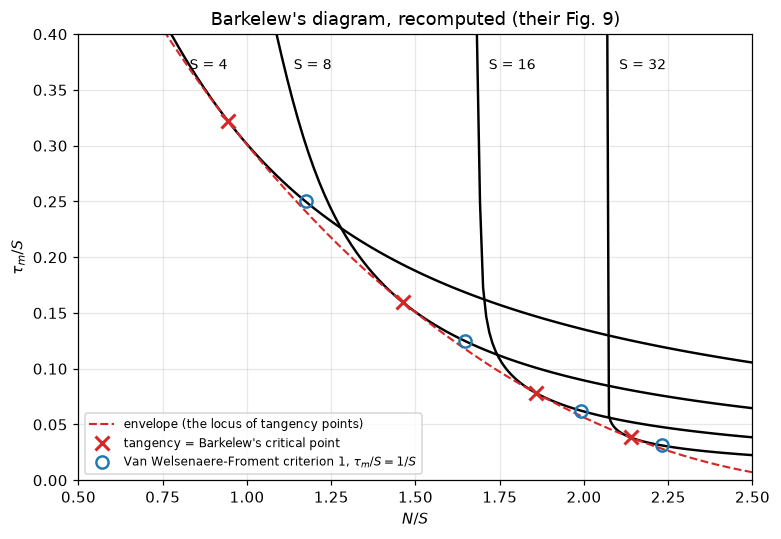
largest tau_m drawn on the diagram: 12.80Does it collapse?
The whole value of the chart is that the tangency points share one \(\tau_m\). The paper says 1.275, for all \(S\). Here is \(\tau_m\) at the tangency over \(S = 3\) to 200 instead of the 4 to 32 Barkelew drew, at the converged step size.
def collapse_table(tan_u, tan_t, one_u, stated=TAU_STATED):
    tab = pd.DataFrame({
        "S": S_WIDE,
        "(N/S) tangency": [tan_u[S] for S in S_WIDE],
        "tau_m tangency": [tan_t[S] for S in S_WIDE],
        "dev from 1.275 %": [(tan_t[S] - stated) / stated * 100 for S in S_WIDE],
        "(N/S) at tau_m=1": [one_u[S] for S in S_WIDE],
        "gap to the right %": [(one_u[S] - tan_u[S]) / tan_u[S] * 100 for S in S_WIDE],
    })
    tab["drawn by Barkelew"] = ["yes" if S in S_PRINTED else "" for S in S_WIDE]
    return tab


TAB = collapse_table(TAN_U, TAN_T, ONE_U)
drawn = TAB[TAB["drawn by Barkelew"] == "yes"]
MAD_DRAWN = drawn["dev from 1.275 %"].abs().mean()
MAD_WIDE = TAB["dev from 1.275 %"].abs().mean()
PEAK_S = float(TAB.S[TAB["tau_m tangency"].idxmax()])
_t = TAB["tau_m tangency"].values
PEAK_MARGIN = float(np.min(_t.max() - np.delete(_t, np.argmax(_t))) / _t.max())
DROP_4_32 = TAN_T[S_PRINTED[0]] - TAN_T[S_PRINTED[-1]]
GAPS = TAB["gap to the right %"].values
print(TAB.to_string(index=False, float_format=lambda v: f"{v:8.4f}")
      + f"\n\nover the four S-curves Barkelew drew : mean |dev| {MAD_DRAWN:.3f} %, "
      + f"tau_m from {drawn['tau_m tangency'].min():.4f} to {drawn['tau_m tangency'].max():.4f}"
      + f"\nover S = {min(S_WIDE):.0f} to {max(S_WIDE):.0f}          : mean |dev| {MAD_WIDE:.3f} %, "
      + f"tau_m from {TAB['tau_m tangency'].min():.4f} to {TAB['tau_m tangency'].max():.4f}"
      + f"\nlargest tau_m at S = {PEAK_S:.0f}; it falls by {DROP_4_32:.4f} from S = 4 to S = 32"
      + f"\nthe gap is positive for {int((GAPS > 0).sum())} of the {len(TAB)} values of S"
      + f"   (range {GAPS.min():.1f} to {GAPS.max():.1f} %)")
S (N/S) tangency tau_m tangency dev from 1.275 % (N/S) at tau_m=1 gap to the right % drawn by Barkelew
3.0000 0.6985 1.2863 0.8837 0.9386 34.3665
4.0000 0.9440 1.2879 1.0128 1.1738 24.3512 yes
6.0000 1.2620 1.2830 0.6255 1.4664 16.1972
8.0000 1.4625 1.2763 0.1055 1.6458 12.5345 yes
12.0000 1.7077 1.2644 -0.8343 1.8612 8.9874
16.0000 1.8563 1.2547 -1.5945 1.9899 7.1975 yes
24.0000 2.0331 1.2400 -2.7418 2.1416 5.3339
32.0000 2.1380 1.2293 -3.5852 2.2309 4.3421 yes
48.0000 2.2609 1.2140 -4.7876 2.3349 3.2714
64.0000 2.3329 1.2031 -5.6375 2.3956 2.6856
100.0000 2.4238 1.1866 -6.9324 2.4719 1.9855
150.0000 2.4883 1.1721 -8.0704 2.5260 1.5136
200.0000 2.5256 1.1622 -8.8498 2.5572 1.2499
over the four S-curves Barkelew drew : mean |dev| 1.575 %, tau_m from 1.2293 to 1.2879
over S = 3 to 200 : mean |dev| 3.512 %, tau_m from 1.1622 to 1.2879
largest tau_m at S = 4; it falls by 0.0586 from S = 4 to S = 32
the gap is positive for 13 of the 13 values of S (range 1.2 to 34.4 %)\(\tau_m\) at the tangency is not a constant. It is largest at \(S = 4\), at the very left edge of the range Barkelew drew, and falls monotonically thereafter, so 1.275 is a good summary of his four curves and a steadily worse one outside them. The panel below shows the drift, and shows how far outside his range it has to be pushed before the collapse stops being usable.
This is not a contradiction of anything the paper asserts. Section 5 says “very close to”, which already declines to claim a constant, and the crosses printed on their Fig. 9 could not have resolved a change of 0.06 in \(\tau_m\) across \(S = 4\)–32 anyway. What the computation supplies is the size of “very close to”, and the fact that it has a sign and a direction.
The second statement in Section 5 survives intact: the point \(\tau_m/S = 1/S\) lies to the right of the tangency for every \(S\) tested, so Van Welsenaere and Froment’s first criterion is more conservative than Barkelew’s everywhere, not merely on the four curves they could see. The size of that margin is not in either paper: it shrinks from 24 % of \(N/S\) at \(S = 4\) to 1.2 % at \(S = 200\).
fig, axes = plt.subplots(1, 2, figsize=(11.4, 4.2))
ax = axes[0]
ax.semilogx(TAB.S, TAB["tau_m tangency"], "o-", color="k", lw=1.6, ms=5)
ax.axhline(TAU_STATED, color="tab:red", ls="--", lw=1.4, label=f"their stated {TAU_STATED}")
ax.axvspan(min(S_PRINTED), max(S_PRINTED), color="tab:blue", alpha=0.10,
           label="the range Barkelew drew")
ax.set(xlabel="$S$", ylabel=r"$\tau_m$ at the tangency",
       title="the collapse, and where it drifts")
ax.legend(fontsize=8)

ax = axes[1]
ax.semilogx(TAB.S, TAB["gap to the right %"], "o-", color="tab:blue", lw=1.6, ms=5)
ax.axhline(0.0, color="k", lw=1.0)
ax.axvspan(min(S_PRINTED), max(S_PRINTED), color="tab:blue", alpha=0.10)
ax.set(xlabel="$S$", ylabel=r"$(N/S)_{\tau_m=1}$ over tangency, %",
       title="how much more conservative criterion 1 is")
fig.tight_layout()
plt.show()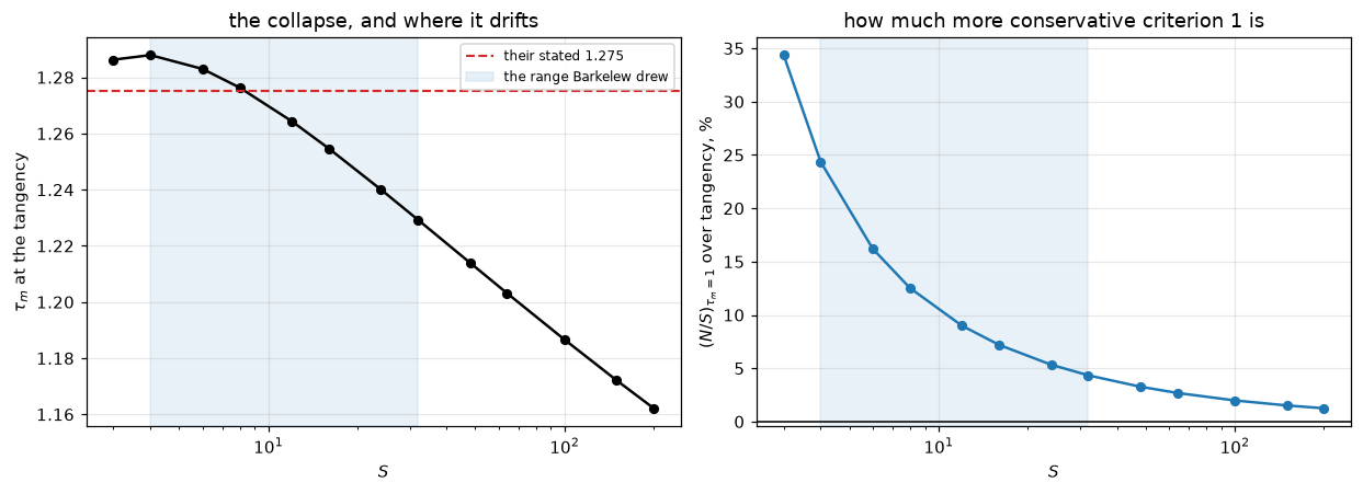
What the two criteria predict for a real tube
\(N\) depends only on the wall temperature and the tube radius; \(S\) carries the inlet pressure. So Barkelew’s criterion, read backwards, gives a critical inlet pressure for any \(T_w\), which is what the circled crosses on their Fig. 8 are. The comparison below recomputes both sides: Barkelew’s tangency locus with his exponential rate law, against Van Welsenaere and Froment’s first criterion back-integrated with the true Arrhenius law, the quantity their Example 1 prints as 0.01651 atm.
# Interpolants over the 13 tangencies of the table: they draw the envelope and
# give each root-find its first bracket, and no published number is read off them.
_LOG_S = np.log(S_WIDE)
_S_OF_N = PchipInterpolator(np.log([TAN_U[S] * S for S in S_WIDE]), _LOG_S)
_S_OF_N_ONE = PchipInterpolator(np.log([ONE_U[S] * S for S in S_WIDE]), _LOG_S)
_U_OF_S = PchipInterpolator(_LOG_S, np.log([TAN_U[S] for S in S_WIDE]))


@lru_cache(maxsize=None)
def s_crit(N):
    """Barkelew's critical S at this N, by a direct root in ln S (model.s_crit_tangency)."""
    S0 = float(np.exp(_S_OF_N(np.log(N))))
    return s_crit_tangency(N, S0 * np.exp(-0.01), S0 * np.exp(0.01),
                           u_guess=lambda S: float(np.exp(_U_OF_S(np.log(S)))))


@lru_cache(maxsize=None)
def s_crit_one(N, level=1.0):
    """S at which tau_m = level at this N (criterion 1 for level 1), a direct root."""
    S0 = float(np.exp(_S_OF_N_ONE(np.log(N))))
    return s_crit_level(N, S0 * np.exp(-0.05), S0 * np.exp(0.05), target=level)


def critical_pressures(case=CASE, T2=None, kk=None, tws=TW_GRID, level=1.0, interp=False):
    """Critical inlet pressures over the wall temperatures, three ways.

    The critical S of both criteria is a direct root at each N. ``T2(Tw)`` is
    the squared reference temperature in tau = a (T - Tw)/T2 and ``kk(Tw)`` the
    rate coefficient at the wall under the same linearisation (default: the
    wall tangent); ``level`` places criterion 1 at tau_m = level. They exist
    for the break tables, as does ``interp=True``, which reads S off the table
    interpolants instead of solving for it.
    """
    T2 = (lambda Tw: Tw ** 2) if T2 is None else T2
    kk = (lambda Tw: float(kexp(case, Tw))) if kk is None else kk
    rows = []
    for Tw in tws:
        N = float(case.C / (case.A * kk(Tw)))
        if interp:
            Sb, S1 = (float(np.exp(f(np.log(N)))) for f in (_S_OF_N, _S_OF_N_ONE))
        else:
            Sb, S1 = s_crit(N), s_crit_one(N, level)
        p0 = lambda S: S * case.A * T2(Tw) / (case.a * case.B)
        rows.append((Tw, N, Sb, p0(Sb), p0(S1), p0_crit_vwf(case, Tw)))
    cmp = pd.DataFrame(rows, columns=["Tw", "N", "S_crit", "p0 Barkelew",
                                      "p0 crit-1 (exp law)", "p0 VWF exact (true law)"])
    cmp["dev Barkelew vs VWF %"] = ((cmp["p0 Barkelew"] - cmp["p0 VWF exact (true law)"])
                                    / cmp["p0 VWF exact (true law)"] * 100)
    return cmp


def crossing(case=CASE):
    """Wall temperature at which Barkelew's and the true-law criterion 1 cross."""
    gap = lambda Tw: float(critical_pressures(case, tws=[Tw])["dev Barkelew vs VWF %"].iloc[0])
    return brentq(gap, 600.0, 700.0, xtol=1e-4), gap(600.0), gap(700.0)


CMP = critical_pressures()
I625 = int(np.argmin(np.abs(CMP.Tw.values - 625.0)))
P0_VWF_625 = CMP["p0 VWF exact (true law)"][I625]
P0_BK_625 = CMP["p0 Barkelew"][I625]
VWF_VS_PRINTED = abs(P0_VWF_625 - V["p0_crit_1_at_Tw625"]) / V["p0_crit_1_at_Tw625"] * 100
DEV_625 = CMP["dev Barkelew vs VWF %"][I625]
DEV_MEAN = CMP["dev Barkelew vs VWF %"].abs().mean()
DEV_WORST = CMP["dev Barkelew vs VWF %"].abs().max()
TW_CROSS, GAP_600, GAP_700 = crossing()
CMP_INTERP = critical_pressures(interp=True)
INTERP_GAP = float(((CMP_INTERP["p0 Barkelew"] - CMP["p0 Barkelew"]).abs()
                    / CMP["p0 Barkelew"]).max())
print(CMP[CMP.Tw.isin([600., 625., 650., 675., 700.])].to_string(
          index=False, float_format=lambda v: f"{v:10.5f}")
      + f"\n\nat Tw = 625 K, their Example 1 prints (p0)_cr,1 = {V['p0_crit_1_at_Tw625']} atm"
      + f"\n  this page's back-integration of the same criterion : {P0_VWF_625:.5f} atm  "
      + f"({VWF_VS_PRINTED:.3f} %)"
      + f"\n  Barkelew's criterion, recomputed                   : {P0_BK_625:.5f} atm  "
      + f"({DEV_625:+.2f} % against it)"
      + f"\n\nover Tw = 600-700 K: mean |dev| {DEV_MEAN:.3f} %, worst {DEV_WORST:.3f} %, "
      + f"signed range {CMP['dev Barkelew vs VWF %'].min():+.2f} to "
      + f"{CMP['dev Barkelew vs VWF %'].max():+.2f} %"
      + f"\nthe two methods cross at Tw = {TW_CROSS:.2f} K (bracketed: {GAP_600:+.2f} % "
      + f"at 600 K, {GAP_700:+.2f} % at 700 K)"
      + "\n\nThe critical S is a root at each N; read off the interpolant through the 13"
      + "\ntangencies instead (as the plots are drawn) it differs by below 2e-3 of p0 "
      + f"(here {INTERP_GAP:.1e}).")
Tw N S_crit p0 Barkelew p0 crit-1 (exp law) p0 VWF exact (true law) dev Barkelew vs VWF %
600.00000 119.52359 52.33538 0.03314 0.03224 0.03395 -2.37806
625.00000 48.15606 23.73644 0.01631 0.01559 0.01651 -1.21010
650.00000 20.80740 12.13909 0.00902 0.00843 0.00899 0.36485
675.00000 9.56708 6.98151 0.00560 0.00510 0.00548 2.20525
700.00000 4.64991 4.48304 0.00386 0.00343 0.00371 4.05651
at Tw = 625 K, their Example 1 prints (p0)_cr,1 = 0.01651 atm
this page's back-integration of the same criterion : 0.01651 atm (0.005 %)
Barkelew's criterion, recomputed : 0.01631 atm (-1.21 % against it)
over Tw = 600-700 K: mean |dev| 1.767 %, worst 4.057 %, signed range -2.38 to +4.06 %
the two methods cross at Tw = 644.67 K (bracketed: -2.38 % at 600 K, +4.06 % at 700 K)
The critical S is a root at each N; read off the interpolant through the 13
tangencies instead (as the plots are drawn) it differs by below 2e-3 of p0 (here 9.0e-04).The two approximations, separated
Section 5’s comparison mixes two different things: Barkelew’s criterion (the envelope tangency instead of \(\tau_m = 1\)) and Barkelew’s rate law (the exponential instead of the true Arrhenius factor). Their Fig. 8 puts his values next to theirs and the text says the two “agree extremely well”, but a reader cannot tell how much of whatever difference remains is which. The paper does say his values were obtained “using the modified rate equation”, so it is not hiding the mixture; it simply does not decompose it.
Computing the intermediate case (their criterion, his rate law) separates them exactly, because the critical \(p^0\) factorises into the two steps:
\[ \frac{p^0_{\mathrm{Barkelew}}}{p^0_{\mathrm{VWF,\ true}}} = \underbrace{\frac{p^0_{\tau_m=1,\ \mathrm{exp}}}{p^0_{\mathrm{VWF,\ true}}}}_{\text{rate law alone}} \times \underbrace{\frac{p^0_{\mathrm{Barkelew}}}{p^0_{\tau_m=1,\ \mathrm{exp}}}}_{\text{criterion alone}} \]
The second factor is the ratio of the critical \(S\) at the tangency to the critical \(S\) at \(\tau_m = 1\) at the same \(N\): a purely dimensionless quantity, so it does not inherit the reconstruction at all. Only the first factor does.
def decompose(cmp):
    dec = pd.DataFrame({"Tw": cmp.Tw})
    dec["rate law alone %"] = (cmp["p0 crit-1 (exp law)"]
                               / cmp["p0 VWF exact (true law)"] - 1.0) * 100
    dec["criterion alone %"] = (cmp["p0 Barkelew"] / cmp["p0 crit-1 (exp law)"] - 1.0) * 100
    dec["total %"] = cmp["dev Barkelew vs VWF %"]
    dec["product of the two %"] = ((1 + dec["rate law alone %"] / 100)
                                   * (1 + dec["criterion alone %"] / 100) - 1) * 100
    return dec


def decomposition_margins(dec):
    """Smallest component magnitude (opposite signs) and smallest lead of the
    smaller component over the total (total smaller than both), in points."""
    r, c, t = (dec[k].values for k in ("rate law alone %", "criterion alone %", "total %"))
    return (np.where(r * c < 0, np.minimum(abs(r), abs(c)), -np.minimum(abs(r), abs(c))),
            np.minimum(abs(r), abs(c)) - abs(t))


DEC = decompose(CMP)
OPP, LEAD = decomposition_margins(DEC)
PRODUCT_GAP = float((DEC["product of the two %"] - DEC["total %"]).abs().max())
print("what the Barkelew-vs-VWF disagreement is made of\n"
      + DEC[DEC.Tw.isin([600., 625., 650., 675., 700.])].to_string(
          index=False, float_format=lambda v: f"{v:9.4f}")
      + f"\n\nrate law alone : {DEC['rate law alone %'].min():+.2f} to "
      + f"{DEC['rate law alone %'].max():+.2f} % (conservative everywhere)"
      + f"\ncriterion alone: {DEC['criterion alone %'].min():+.2f} to "
      + f"{DEC['criterion alone %'].max():+.2f} % (the other way everywhere)"
      + f"\ntotal          : {DEC['total %'].min():+.2f} to {DEC['total %'].max():+.2f} %"
      + f"\nopposite sign at {int((OPP > 0).sum())} of the {len(DEC)} wall temperatures"
      + f" (smallest component {OPP.min():.2f} points)"
      + f"\ntotal smaller in magnitude than BOTH components at {int((LEAD > 0).sum())} of them"
      + f" (smallest lead {LEAD.min():.2f} points)"
      + "\nthe product of the two reproduces the total to below 1e-10 points "
      + f"(here {PRODUCT_GAP:.1e}),"
      + "\nas it must: the decomposition is exact, not a fit.")
what the Barkelew-vs-VWF disagreement is made of
Tw rate law alone % criterion alone % total % product of the two %
600.0000 -5.0513 2.8155 -2.3781 -2.3781
625.0000 -5.5702 4.6173 -1.2101 -1.2101
650.0000 -6.1928 6.9906 0.3649 0.3649
675.0000 -6.9094 9.7912 2.2052 2.2052
700.0000 -7.6951 12.7313 4.0565 4.0565
rate law alone : -7.70 to -5.05 % (conservative everywhere)
criterion alone: +2.82 to +12.73 % (the other way everywhere)
total : -2.38 to +4.06 %
opposite sign at 21 of the 21 wall temperatures (smallest component 2.82 points)
total smaller in magnitude than BOTH components at 21 of them (smallest lead 0.44 points)
the product of the two reproduces the total to below 1e-10 points (here 1.8e-14),
as it must: the decomposition is exact, not a fit.fig, axes = plt.subplots(1, 2, figsize=(11.4, 4.2))
ax = axes[0]
ax.plot(CMP.Tw, CMP["p0 VWF exact (true law)"], "k-", lw=2.0,
label="VWF criterion 1, true rate law (exact)")
ax.plot(CMP.Tw, CMP["p0 Barkelew"], "--", color="tab:red", lw=1.8,
label="Barkelew's tangency, exponential rate law")
ax.plot(CMP.Tw, CMP["p0 crit-1 (exp law)"], ":", color="tab:blue", lw=1.8,
label=r"VWF criterion 1 in Barkelew's variables ($\tau_m=1$)")
ax.plot([625.0], [V["p0_crit_1_at_Tw625"]], "*", color="k", ms=13,
label="their Example 1, printed")
ax.set(xlabel="$T_w$ (K)", ylabel="critical $p^0$ (atm)", xlim=(600, 700),
yscale="log", title="the runaway boundary, three ways")
ax.legend(fontsize=8)
ax = axes[1]
ax.plot(DEC.Tw, DEC["rate law alone %"], ":", color="tab:blue", lw=1.8,
label="rate law alone (exponential vs true)")
ax.plot(DEC.Tw, DEC["criterion alone %"], "-.", color="tab:green", lw=1.8,
label=r"criterion alone (tangency vs $\tau_m = 1$)")
ax.plot(DEC.Tw, DEC["total %"], "-", color="tab:red", lw=2.0,
label="total, Barkelew vs VWF exact")
ax.axhline(0.0, color="k", lw=1.0)
ax.axvline(TW_CROSS, color="k", ls=":", lw=1.0)
ax.annotate(f"cross at {TW_CROSS:.1f} K", (TW_CROSS, 8.0), fontsize=8, ha="center")
ax.set(xlabel="$T_w$ (K)", ylabel="deviation, %", xlim=(600, 700),
title="what the disagreement is made of")
ax.legend(fontsize=8)
fig.tight_layout()
plt.show()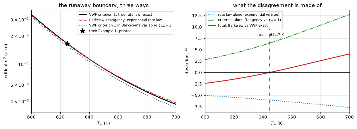
The two methods cross. Barkelew’s chart is more conservative than the true-rate criterion at low wall temperature (it allows a lower inlet pressure) and less conservative at high, and the decomposition says why. The exponential rate law on its own is conservative everywhere and by more than the total discrepancy; the tangency criterion sits above \(\tau_m = 1\) and pushes the other way by a growing amount. The two have opposite sign at every wall temperature and the total is smaller in magnitude than either component at all of them. That is the honest reading of “agree extremely well”: the agreement is better than either approximation taken alone, and it is better for a reason neither paper states.
How much earlier the simplified rate law runs away
Their Fig. 3 and their Fig. 10 are the same four cases, \(p^0 = 0.017\) atm and \(T_w = 625, 626, 627, 628\) K, with the true rate law and with Barkelew’s. The text says the modified equation “leads to runaway well before the true rate equation”. This is what that costs. The hot spot with the true law is computed twice: by the pymrm Tube on 2000 cells and refined to 16000, and by marching the same equations as an initial-value problem.
P0_FIG = V["fig10_p0"]
TW_FIG = [V[f"fig10_Tw_{i}"] for i in (1, 2, 3, 4)]
T_TOP, Z_TOP = V["fig10_T_max"], V["fig10_z_max"]


def tube_hot_spots(case=CASE, p0=P0_FIG, ns=N_TUBE_STUDY, tws=TW_FIG):
    """pymrm hot spot (K) of the true-law tube on each grid, per wall temperature."""
    return {Tw: [Tube(case, p0, Tw, n_z=n).solve().hot_spot() for n in ns] for Tw in tws}


def runaways(case=CASE, p0=P0_FIG, tws=TW_FIG):
    """March both rate laws; runaway = reaching the top of the printed axis."""
    out = []
    for Tw in tws:
        zt, Tt, zt_top = profile_ivp(case, p0, Tw, False, T_stop=T_TOP)
        zs, Ts, zs_top = profile_ivp(case, p0, Tw, True, T_stop=T_TOP)
        out.append(dict(Tw=Tw, zt=zt, Tt=Tt, zt_top=zt_top, zs=zs, Ts=Ts, zs_top=zs_top))
    return out


def runaway_counts(runs):
    """Runaways with the true and with the exponential law, and the margin of
    the classification: relative distance to 800 K (no runaway) or to the
    tube end (runaway), the smaller."""
    n_true = sum(r["zt_top"] is not None for r in runs)
    n_exp = sum(r["zs_top"] is not None for r in runs)
    m = [(T_TOP - r["Tt"].max()) / T_TOP if r["zt_top"] is None else (Z_TOP - r["zt_top"]) / Z_TOP
         for r in runs] + \
        [(T_TOP - r["Ts"].max()) / T_TOP if r["zs_top"] is None else (Z_TOP - r["zs_top"]) / Z_TOP
         for r in runs]
    return n_true, n_exp, float(min(m))


RUNS = runaways()
HS = tube_hot_spots()
N_TRUE, N_EXP, RUN_MARGIN = runaway_counts(RUNS)

fig, axes = plt.subplots(1, 2, figsize=(11.4, 4.4), sharey=True)
for r, col in zip(RUNS, ["tab:blue", "tab:green", "tab:orange", "tab:red"]):
    axes[0].plot(r["zt"], r["Tt"], color=col, lw=1.7, label=f"$T_w$ = {r['Tw']:.0f} K")
    axes[1].plot(r["zs"], r["Ts"], color=col, lw=1.7, label=f"$T_w$ = {r['Tw']:.0f} K")
for ax, ttl in zip(axes, ["true rate law (their Fig. 3)",
                          "Barkelew's exponential (their Fig. 10)"]):
    ax.set(xlabel="$z'$ (m)", xlim=(0.0, Z_TOP), ylim=(600.0, T_TOP), title=ttl)
    ax.legend(fontsize=8, loc="upper left")
axes[0].set_ylabel("$T$ (K)")
axes[0].text(0.55, 620, f"$p^0$ = {P0_FIG} atm", fontsize=9)
fig.tight_layout()
plt.show()

f3 = pd.DataFrame({"Tw": TW_FIG})
for j, n in enumerate(N_TUBE_STUDY):
    f3[f"pymrm n={n}"] = [HS[Tw][j] for Tw in TW_FIG]
f3["Richardson (8000, 16000)"] = 2 * f3["pymrm n=16000"] - f3["pymrm n=8000"]
f3["marched"] = [float(r["Tt"].max()) for r in RUNS]
f3[f"dev n={N_TUBE} %"] = ((f3[f"pymrm n={N_TUBE}"] - f3["marched"]).abs() / f3["marched"] * 100)
f3["z' at 800 K, exponential law (m)"] = [r["zs_top"] for r in RUNS]
_hs628 = np.array(HS[TW_FIG[-1]])
TUBE_ORDER = float(np.log2((_hs628[1] - _hs628[0]) / (_hs628[2] - _hs628[1])))
TUBE_DEV_WORST = float(f3[f"dev n={N_TUBE} %"].max())
TUBE_RICH_GAP = float((f3["Richardson (8000, 16000)"] - f3["marched"]).abs().max())
print(f3.to_string(index=False, float_format=lambda v: f"{v:9.4f}")
      + f"\n\nThe pymrm tube converges at first order to the marched hot spot (observed order"
      + f"\n{TUBE_ORDER:.2f} at {TW_FIG[-1]:.0f} K from 2000, 4000, 8000 cells), and the Richardson value"
      + "\nfrom 8000 and 16000 cells meets the march to below 0.05 K "
      + f"(here {TUBE_RICH_GAP:.1e} K)."
      + f"\nThe {TUBE_DEV_WORST:.2f} % at {TW_FIG[-1]:.0f} K on {N_TUBE} cells is grid error where the profile is steep."
      + f"\nWith the true rate law {N_TRUE} of the four cases reach {T_TOP:.0f} K inside the tube;"
      + f"\nwith Barkelew's exponential {N_EXP} of the same four reach the top of the paper's"
      + "\ntemperature axis before the end of the tube, which is what their Fig. 10 shows,"
      + "\nand why his chart is conservative.")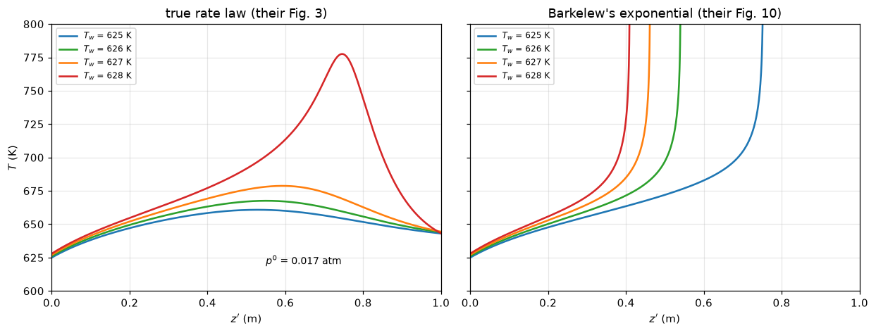
       Tw  pymrm n=2000  pymrm n=4000  pymrm n=8000  pymrm n=16000  Richardson (8000, 16000)   marched  dev n=2000 %  z' at 800 K, exponential law (m)
 625.0000      660.7792      660.8018      660.8132       660.8189                  660.8245  660.8245        0.0069                            0.7511
 626.0000      667.4837      667.5190      667.5367       667.5456                  667.5545  667.5544        0.0106                            0.5398
 627.0000      678.5868      678.6607      678.6977       678.7163                  678.7348  678.7348        0.0218                            0.4613
 628.0000      770.8533      774.1730      775.8644       776.7172                  777.5701  777.5745        0.8644                            0.4090

The pymrm tube converges at first order to the marched hot spot (observed order
0.97 at 628 K from 2000, 4000, 8000 cells), and the Richardson value
from 8000 and 16000 cells meets the march to below 0.05 K (here 4.4e-03 K).
The 0.86 % at 628 K on 2000 cells is grid error where the profile is steep.
With the true rate law 0 of the four cases reach 800 K inside the tube;
with Barkelew's exponential 4 of the same four reach the top of the paper's
temperature axis before the end of the tube, which is what their Fig. 10 shows,
and why his chart is conservative.
The one printed object that can discriminate the reconstruction
Everything checked so far lives either inside the reduced system, which contains no reference temperature at all, or compares two criteria against each other. None of it can settle the one step of the reconstruction that the paper does not print: the temperature at which the exponent is linearised.
Their Fig. 10 can, because it is drawn with the simplified rate law, and the position at which each curve leaves the top of the printed 800 K axis depends on that choice directly. The previous cell already computed those four positions. Comparing them is the decisive test, and it is the only one available.
Review status: not yet page evidence. The four positions on the printed figure are curve positions read off a scan, not values the paper prints, so under this repository’s rules they are a figure digitisation and need the maintainer’s visual review before they can count. They were measured by
queue_cases/D2.1/review/extract_figure10.py, which writes a numbered overlay for that review; they are not in either committed CSV and nothing else on this page depends on them. The case file carries a non-blocking follow-up asking for the review. Until it happens, read the next table as an indication. The reconstruction stands on the printed sentences either way; this only makes it decisive rather than merely consistent.
# ---------------------------------------------------------------------------
# QUARANTINE: the only numbers on this page taken off a curve rather than out
# of the text. Measured on a 600 dpi render of journal page 1512 by
# queue_cases/D2.1/review/extract_figure10.py, which fits each of the six marks
# (two frame edges, four curves) linearly over 72 clean rows and extrapolates to
# the top frame row where T = 800 K actually is; worst fit residual 1.5 px. The
# frame there is x = 575.5 px (z' = 0) and x = 2154.3 px (z' = 1.0 m, the
# printed axis limits), the four curves cross it at x = 1220.0, 1321.5, 1435.6
# and 1768.2 px, and the printed 0.5 tick lands 0.03 % of full scale from the
# frame midpoint. AWAITING MAINTAINER VISUAL REVIEW of the overlay that script
# writes: not in any CSV, no sidecar, and no other cell reads this dict.
FIG10_MEASURED_PENDING_REVIEW = {628.0: 0.4082, 627.0: 0.4725,
                                 626.0: 0.5448, 625.0: 0.7555}


def fig10_table(case=CASE, p0=P0_FIG, rtol=1e-10):
    """Blow-up positions and highest temperatures for every linearisation."""
    rows, hot_rows = [], []
    for Tw in TW_FIG[::-1]:                     # 628, 627, 626, 625
        row = {"Tw": Tw, "figure (pending review)": FIG10_MEASURED_PENDING_REVIEW[Tw]}
        hot = {"Tw": Tw}
        for nm, (kw, sl) in linearisations(case, Tw).items():
            z, Tmax = blowup_z(case, Tw, kw, sl, p0, length=Z_TOP, T_stop=T_TOP, rtol=rtol)
            row[nm] = z if z is not None else np.nan
            hot[nm] = Tmax
        rows.append(row)
        hot_rows.append(hot)
    fig10, hottest = pd.DataFrame(rows), pd.DataFrame(hot_rows)
    devs = pd.DataFrame({"Tw": fig10.Tw})
    for nm in linearisations(case, 625.0):
        devs[nm] = (fig10[nm] - fig10["figure (pending review)"]) \
            / fig10["figure (pending review)"] * 100
    return fig10, hottest, devs


def fig10_summary(fig10, hottest, devs):
    names = list(devs.columns[1:])
    page, alt = names[0], names[1:3]          # the wall tangent; the two permitted others
    d_page = devs[page].abs().values
    alt_d = np.concatenate([devs[nm].abs().dropna().values for nm in alt])
    n_run = {nm: int(fig10[nm].notna().sum()) for nm in names}
    # runaway margin: relative distance to 800 K (none) or to the tube end (runaway)
    marg = min(min((T_TOP - hottest[nm][fig10[nm].isna()]).min() / T_TOP
                   if fig10[nm].isna().any() else np.inf,
                   (Z_TOP - fig10[nm].dropna()).min() / Z_TOP
                   if fig10[nm].notna().any() else np.inf) for nm in names)
    return dict(page_worst=float(d_page.max()),
                n_under_1=int((d_page < 1.0).sum()),
                under_1_margin=float(np.min(np.abs(d_page - 1.0))),
                alt_min=float(alt_d.min()) if alt_d.size else np.nan,   # nan: none ran away
                alt_max=float(alt_d.max()) if alt_d.size else np.nan,
                n_run=n_run, run_margin=float(marg),
                square_z_max_mm=float(fig10[names[3]].max() * 1e3))


FIG10, HOTTEST, DEVS = fig10_table()
F10 = fig10_summary(FIG10, HOTTEST, DEVS)
LSODA_Z = [r["zs_top"] for r in RUNS][::-1]                 # 628 -> 625
RADAU_Z = list(FIG10["tangent at T_w  (this page)"])
LSODA_RADAU = max(abs(a - b) for a, b in zip(LSODA_Z, RADAU_Z))
lines = [f"z' (m) at which T reaches the printed 800 K axis, p0 = {P0_FIG} atm; "
         f"NaN = no runaway within the printed {Z_TOP:.0f} m",
         FIG10.to_string(index=False, float_format=lambda v: f"{v:8.4f}"),
         "", "deviation from the measured positions, %",
         DEVS.to_string(index=False, float_format=lambda v: f"{v:8.2f}"), ""]
for nm, n_ok in F10["n_run"].items():
    if n_ok == 0:
        lines.append(f"  {nm:30s} no runaway in any of the four cases")
    else:
        lines.append(f"  {nm:30s} {n_ok}/4 run away, |dev| {DEVS[nm].abs().min():.1f} "
                     f"to {DEVS[nm].abs().max():.1f} %")
lines += ["", "highest T reached inside the printed tube, K (800 = ran away)",
          HOTTEST.to_string(index=False, float_format=lambda v: f"{v:8.2f}"), "",
          "Not an integrator artefact: the LSODA march in z' that drew the figure above",
          "  gives " + ", ".join(f"{z:.4f}" for z in LSODA_Z) + " m",
          "  Radau in the phase plane here gives " + ", ".join(f"{z:.4f}" for z in RADAU_Z) + " m",
          f"  worst difference below 1e-6 m (here {LSODA_RADAU:.1e} m)",
          "", "With the square dropped every case ignites at the inlet: 800 K is reached by",
          f"z' = {F10['square_z_max_mm']:.2f} mm at the latest. A march in z' cannot follow that "
          "ignition (Radau",
          "stops on a step below the spacing of floating-point numbers); the phase-plane",
          "route, with the partial pressure as the independent variable, keeps both",
          "right-hand sides finite and does."]
print("\n".join(lines))
z' (m) at which T reaches the printed 800 K axis, p0 = 0.017 atm; NaN = no runaway within the printed 1 m
Tw figure (pending review) tangent at T_w (this page) tangent at T_M chord T_w to T_M square dropped, a(T-T_w)/T_w
628.0000 0.4082 0.4090 0.5608 0.5285 0.0002
627.0000 0.4725 0.4613 NaN 0.7522 0.0003
626.0000 0.5448 0.5398 NaN NaN 0.0003
625.0000 0.7555 0.7511 NaN NaN 0.0003
deviation from the measured positions, %
Tw tangent at T_w (this page) tangent at T_M chord T_w to T_M square dropped, a(T-T_w)/T_w
628.00 0.21 37.38 29.48 -99.94
627.00 -2.36 NaN 59.19 -99.95
626.00 -0.91 NaN NaN -99.95
625.00 -0.58 NaN NaN -99.96
tangent at T_w (this page) 4/4 run away, |dev| 0.2 to 2.4 %
tangent at T_M 1/4 run away, |dev| 37.4 to 37.4 %
chord T_w to T_M 2/4 run away, |dev| 29.5 to 59.2 %
square dropped, a(T-T_w)/T_w 4/4 run away, |dev| 99.9 to 100.0 %
highest T reached inside the printed tube, K (800 = ran away)
Tw tangent at T_w (this page) tangent at T_M chord T_w to T_M square dropped, a(T-T_w)/T_w
628.00 800.00 800.00 800.00 800.00
627.00 800.00 683.48 800.00 800.00
626.00 800.00 668.31 668.85 800.00
625.00 800.00 661.14 660.62 800.00
Not an integrator artefact: the LSODA march in z' that drew the figure above
gives 0.4090, 0.4613, 0.5398, 0.7511 m
Radau in the phase plane here gives 0.4090, 0.4613, 0.5398, 0.7511 m
worst difference below 1e-6 m (here 3.6e-08 m)
With the square dropped every case ignites at the inlet: 800 K is reached by
z' = 0.27 mm at the latest. A march in z' cannot follow that ignition (Radau
stops on a step below the spacing of floating-point numbers); the phase-plane
route, with the partial pressure as the independent variable, keeps both
right-hand sides finite and does.The wall tangent reproduces all four printed positions, three of them to under one percent and the fourth to 2.4 %. Every alternative that the printed sentences permit fails qualitatively, not marginally. Linearising at \(T_M\), or on the chord from \(T_w\) to \(T_M\), weakens the temperature dependence enough that most of the four cases never reach 800 K at all inside the printed 1 m of tube (three of four for the \(T_M\) tangent, two of four for the chord), and the ones that do run away are off by 29 to 59 %. Dropping the square goes the other way and makes the exponent so steep that every case ignites at the inlet: none of the four stays below 800 K, and all of them reach it within the first 0.3 mm of tube, against 0.4 to 0.8 m in the figure.
So the reconstruction is not merely consistent with the printed text: subject to the maintainer’s review of those four positions, it is the only member of its family that reproduces the paper’s own figure.
Validation
Ranked before any code was written. The paper offers no experiment, so the highest available route is a stated numerical result in the text, and Section 5 has exactly one, \(\tau_m = 1.275\) at the tangency, plus one stated identity, \(\tau_m = 1\) for the other criterion. No figure was digitised into the page’s data; the only things taken from Figs. 9 and 10 into the CSVs are the labels printed inside them, and the four Fig. 10 positions above are quarantined and awaiting review.
| # | check | what it tests | what it cannot see |
|---|---|---|---|
| 1 | \(\tau_m\) at the envelope tangency against their 1.275 | the exponential temperature dependence, and the choice of \(N/S\) and \(\tau_m/S\) as the collapsing groups | the dimensional definitions of \(N\) and \(S\) (the reduced system does not contain them) and, as measured below, all but a little of the reaction order |
| 2 | the \(\tau_m = 1\) point lies right of the tangency, every \(S\) | the sign and ordering claim of Section 5 | magnitude; it is a sign test |
| 3 | Barkelew’s critical \(p^0\) against the criterion 1 back-integration | the dimensional group definitions and the reference temperature | nothing about \(B\): it is invariant under any rescaling of \(B\) down to floating point, structurally and not by luck, hence blind to \((-\Delta H)\), \(\rho_b\) and \(p_B^0\), measured below. It is also nearly blind to \(C\), including the \(c_p\rho_g\) trap, which check 5 catches instead |
| 4 | pymrm against the phase-plane quadrature | the operator assembly, the discretisation, and the reduced model as the finite-volume route transcribes it: the two routes do not share a reaction function, and a defect in BarkelewTube.reaction alone makes the pymrm solve fail, measured below |
a defect written identically into both transcriptions, and everything dimensional: it lives entirely inside the reduced system |
| 5 | the parameter reading against four printed derived quantities | a lost decimal point anywhere in the table, and the \(c_p\rho_g\) trap | none of the model |
Checks 1 and 3 are the ones that carry weight, and they are blind to different things: 1 lives entirely inside the dimensionless system and cannot see a wrong \(N\) or \(S\); 3 is built on those definitions but cannot see anything that cancels between its two routes. The tables below measure both claims rather than asserting them.
# Check 4: the pymrm reactor against the phase-plane quadrature, at the four
# tangency points, plus the observed order of convergence.
def check4_table(ns=N_ZETA_STUDY, **kw):
    rows = []
    for S in S_PRINTED:
        N = TAN_U[S] * S
        ref = tau_max_phase(N, S)
        errs = [abs(tau_max_pymrm(N, S, n_z=n, **kw) - ref) / ref * 100 for n in ns]
        order = -np.polyfit(np.log(ns), np.log(errs), 1)[0] if len(ns) > 1 else np.nan
        rows.append((S, ref, *errs, order))
    return pd.DataFrame(rows, columns=["S", "tau_m reference"]
                        + [f"err {n} %" for n in ns] + ["observed order"])


CONV4 = check4_table()
CROSS_MEAN = CONV4[f"err {N_ZETA} %"].mean()
CROSS_WORST = CONV4[f"err {N_ZETA} %"].max()
ORDER4 = CONV4["observed order"].mean()
print("4. pymrm (finite volume in zeta) vs phase-plane quadrature (adaptive, no grid)\n"
      + CONV4.to_string(index=False, float_format=lambda v: f"{v:9.4f}")
      + f"\n\nmean |dev| at n_zeta = {N_ZETA}: {CROSS_MEAN:.3f} %, worst {CROSS_WORST:.3f} %; "
      + f"first-order upwind, so O(h) is\nthe expected order and {ORDER4:.2f} is what comes out.")
4. pymrm (finite volume in zeta) vs phase-plane quadrature (adaptive, no grid)
S tau_m reference err 200 % err 400 % err 800 % err 1600 % observed order
4.0000 1.2879 1.4816 0.7473 0.3749 0.1878 0.9936
8.0000 1.2763 1.8958 0.9591 0.4820 0.2417 0.9907
16.0000 1.2547 2.2104 1.1228 0.5660 0.2842 0.9866
32.0000 1.2293 2.5114 1.2845 0.6507 0.3275 0.9798
mean |dev| at n_zeta = 1600: 0.260 %, worst 0.328 %; first-order upwind, so O(h) is
the expected order and 0.99 is what comes out.Make sure the checks can fail
Each check is now given a defect it is presented as guarding against, and one it is not. A number that does not move is decoration; the point of printing this table is to say which cells are which, and one row below is printed precisely because it cannot fail. Every defect re-runs the computation behind its check; a computation that stops (no envelope, no sign change, a reactor solve that does not converge) is reported as such, never as a number.
import warnings

# The defect rows below drive the reactor into overflow on purpose; the
# warnings that produces are not results, so they are silenced for the rest
# of the page.
warnings.filterwarnings("ignore", category=RuntimeWarning)


def check1(tm=None, Ss=S_PRINTED):
    """mean |dev| of tau_m at the tangency from their 1.275 over the four
    S-curves Barkelew drew; None when the envelope ceases to exist."""
    d = []
    for S in Ss:
        _, t = tangency(S, tm)
        if t is None:
            return None
        d.append(abs(t - TAU_STATED) / TAU_STATED * 100)
    return float(np.mean(d))


def check3(T2=None, kk=None, case=CASE):
    """mean |dev| of Barkelew's critical p0 from the criterion 1 exact value."""
    return float(critical_pressures(case, T2=T2, kk=kk)["dev Barkelew vs VWF %"].abs().mean())


def check4(n_z=N_ZETA, **kw):
    """mean |dev| of the pymrm hot spot from the quadrature at the tangencies."""
    return float(check4_table(ns=(n_z,), **kw)[f"err {n_z} %"].mean())


def check5(case):
    return float(parameter_reading(case)["dev %"].max())


def attempt(fn):
    """Run a defect and say HOW it fails, not merely that it did. Returns the
    number (nan when the computation stops) and its description."""
    try:
        v = fn()
    except NewtonBreakdown:
        return np.nan, "a pymrm solve breaks down (singular Jacobian)"
    except RuntimeError:
        return np.nan, "a pymrm solve does not converge"
    except ValueError:
        return np.nan, "brentq bracketing fails (ValueError)"
    if v is None:
        return np.nan, "no sign change: the envelope is gone"
    return v, f"{v:.3f} %"


def pymrm_outcomes(**kw):
    """Per printed S: the pymrm hot spot with a defect, or why there is none."""
    out = []
    for S in S_PRINTED:
        try:
            out.append(f"S = {S:.0f}: {tau_max_pymrm(TAN_U[S] * S, S, n_z=N_ZETA, **kw):.3g}")
        except NewtonBreakdown:
            out.append(f"S = {S:.0f}: Newton breaks down")
        except RuntimeError:
            out.append(f"S = {S:.0f}: Newton does not converge")
    return "; ".join(out)


lin = lambda t: 1.0 + t                        # exp(tau) -> 1 + tau
T_M2 = lambda Tw: t_max_peak(CASE, Tw) ** 2
k_at_TM = lambda Tw: float(kexp(CASE, t_max_peak(CASE, Tw))
                           * np.exp(-CASE.a * (t_max_peak(CASE, Tw) - Tw)
                                    / t_max_peak(CASE, Tw) ** 2))
CASE_TRAP = replace(CASE, c_p=CASE.c_p * CASE.rho_g)

BASE1, BASE3, BASE4, BASE5 = MAD_CONV, DEV_MEAN, CROSS_MEAN, check5(CASE)
BASE = {1: BASE1, 3: BASE3, 4: BASE4, 5: BASE5}
C3_TM = check3(T2=T_M2, kk=k_at_TM)
DEFECTS = [
    ("exp(tau) -> 1 + tau in the reduced ODE",
     lambda: check1(lambda N, S, **kw: tau_max_phase(N, S, expo=lin)), 1),
    ("cooling term sign flipped, -N tau -> +N tau",
     lambda: check1(lambda N, S, **kw: tau_max_phase(N, S, cool=-1.0)), 1),
    ("reaction second order in y instead of first",
     lambda: check1(lambda N, S, **kw: tau_max_phase(N, S, order=2.0)), 1),
    ("linearise the rate about T_M instead of T_w", lambda: C3_TM, 3),
    ("cooling sign flipped in BarkelewTube.reaction ONLY", lambda: check4(cool=-1.0), 4),
    ("S 10 % wrong in BarkelewTube.reaction ONLY", lambda: check4(s_fac=1.1), 4),
    ("nu = 1 (cylindrical) in construct_div", lambda: check4(nu=1), 4),
    ("n_zeta = 25 cells", lambda: check4(n_z=25), 4),
    ("c_p multiplied by rho_g (the page's own headline trap)", lambda: check5(CASE_TRAP), 5),
]
OUT = {name: attempt(fn) for name, fn, _ in DEFECTS}
brk_tab = pd.DataFrame([(name, which, f"{BASE[which]:.3f} %", OUT[name][1])
                        for name, _, which in DEFECTS],
                       columns=["injected defect", "check", "before", "after"])
print("defects each check is presented as guarding against\n" + brk_tab.to_string(index=False)
      + "\n\nthe two BarkelewTube.reaction rows, per S:"
      + "\n  cooling sign flipped: " + pymrm_outcomes(cool=-1.0)
      + "\n  S 10 % high         : " + pymrm_outcomes(s_fac=1.1))
defects each check is presented as guarding against
injected defect check before after
exp(tau) -> 1 + tau in the reduced ODE 1 1.575 % no sign change: the envelope is gone
cooling term sign flipped, -N tau -> +N tau 1 1.575 % brentq bracketing fails (ValueError)
reaction second order in y instead of first 1 1.575 % 1.339 %
linearise the rate about T_M instead of T_w 3 1.767 % 7.210 %
cooling sign flipped in BarkelewTube.reaction ONLY 4 0.260 % a pymrm solve breaks down (singular Jacobian)
S 10 % wrong in BarkelewTube.reaction ONLY 4 0.260 % a pymrm solve does not converge
nu = 1 (cylindrical) in construct_div 4 0.260 % 100.000 %
n_zeta = 25 cells 4 0.260 % 13.396 %
c_p multiplied by rho_g (the page's own headline trap) 5 0.090 % 22.660 %
the two BarkelewTube.reaction rows, per S:
cooling sign flipped: S = 4: Newton breaks down; S = 8: Newton does not converge; S = 16: Newton does not converge; S = 32: Newton does not converge
S 10 % high : S = 4: 1.6; S = 8: 1.91; S = 16: Newton does not converge; S = 32: Newton does not converge# ---- the row that cannot fail, printed as such ------------------------------
# tau = a(T - Tw)/Tw with the square dropped enters check 3 ONLY through the
# factor T2(Tw) in p0 = Sc*A*T2(Tw)/(a*B). kk, N and the interpolated Sc are
# untouched, so p0 is multiplied by exactly 1/Tw and the deviation is
# 1 - p0/(Tw * p_ref) BY CONSTRUCTION. It is arithmetic, not evidence.
SQ_MEASURED = check3(T2=lambda Tw: Tw)
SQ_PREDICTED = float(np.mean(np.abs(CMP["p0 Barkelew"] / CMP.Tw
- CMP["p0 VWF exact (true law)"])
/ CMP["p0 VWF exact (true law)"] * 100))
SQ_GAP = abs(SQ_MEASURED - SQ_PREDICTED)
print("a row that CANNOT fail, printed so it is not mistaken for evidence\n"
+ pd.DataFrame([{
"injected defect": "tau = a(T-T_w)/T_w, the square dropped",
"check": 3, "before": f"{BASE3:.3f} %", "after": f"{SQ_MEASURED:.3f} %",
"predicted from the baseline alone, no ODE re-run": f"{SQ_PREDICTED:.3f} %",
}]).to_string(index=False)
+ f"\nthe two agree to below 1e-9 points (here {SQ_GAP:.1e}), because they are the "
+ "same arithmetic:"
+ f"\n p0 is multiplied by exactly 1/T_w ~ 1/{CMP.Tw.mean():.0f}, so the deviation is "
+ f"forced to be about {100 * (1 - 1 / CMP.Tw.mean()):.2f} %"
+ "\n whatever the model, the groups or the criterion happen to be. This row"
+ "\n is a units check on one factor; it tests nothing about the reconstruction."
+ "\n The row that DOES test the reconstruction is the T_M linearisation above,"
+ f"\n {BASE3:.3f} % -> {C3_TM:.3f} %, and the Fig. 10 comparison earlier on the page.")a row that CANNOT fail, printed so it is not mistaken for evidence
injected defect check before after predicted from the baseline alone, no ODE re-run
tau = a(T-T_w)/T_w, the square dropped 3 1.767 % 99.845 % 99.845 %
the two agree to below 1e-9 points (here 0.0e+00), because they are the same arithmetic:
p0 is multiplied by exactly 1/T_w ~ 1/650, so the deviation is forced to be about 99.85 %
whatever the model, the groups or the criterion happen to be. This row
is a units check on one factor; it tests nothing about the reconstruction.
The row that DOES test the reconstruction is the T_M linearisation above,
1.767 % -> 7.210 %, and the Fig. 10 comparison earlier on the page.# ---- what each check is blind to, measured -----------------------------------
C3_B11 = check3(case=replace(CASE, minus_dH=CASE.minus_dH * 1.1))
C3_C12 = check3(case=replace(CASE, U=CASE.U * 1.2))
C3_TRAP = check3(case=CASE_TRAP)
C1_ORDER2 = OUT["reaction second order in y instead of first"][0]
B_MOVE = abs(C3_B11 - BASE3) / BASE3 * 100
LNK = parameter_reading(CASE)["recomputed"][1]
LNK_TRAP = parameter_reading(CASE_TRAP)["recomputed"][1]
TRAP5 = check5(CASE_TRAP)
blind = [
("B x 1.1, i.e. (-dH), rho_b or p_B0 10 % wrong", 3, BASE3, C3_B11,
"check 3 sees the heat of reaction"),
("C x 1.2, i.e. U 20 % wrong", 3, BASE3, C3_C12,
"check 3 sees the heat transfer coefficient"),
("c_p multiplied by rho_g (in B and C)", 3, BASE3, C3_TRAP, "check 3 catches the c_p trap"),
("reaction second order in y instead of first", 1, BASE1, C1_ORDER2,
"the 1.275 pins the reaction order"),
]
bl = pd.DataFrame([(n, w, f"{b:.4f} %", f"{a:.4f} %",
"(here %.1e %%)" % (abs(a - b) / b * 100) if n.startswith("B x")
else f"{abs(a - b) / b * 100:.3g} %", c) for n, w, b, a, c in blind],
columns=["injected defect", "check", "before", "after", "relative move",
"claim this page does NOT make"])
print("what the checks are blind to - measured, and named as claims not made\n"
+ bl.to_string(index=False)
+ "\n\nCheck 3 does not move under a rescaling of B beyond floating point (below "
+ "1e-6 %),\nand that is structural, not luck: p0(Barkelew) is proportional to 1/B, and"
+ "\nsubstituting p = q/B removes B from their Eq. 5 and from p_M as well, so"
+ "\np0(VWF) is proportional to 1/B too. The ratio cannot move. Check 3 therefore"
+ "\nsays nothing whatever about (-dH), rho_b or p_B0."
+ "\n\nIt is also nearly blind to C, including the c_p x rho_g trap this page"
+ "\ninherits from D2.2, which lands inside anything a reader would call"
+ "\nagreement. That trap is caught by CHECK 5, not check 3: the recomputed"
+ f"\nln K goes from {LNK:.4f} to {LNK_TRAP:.4f} against the printed {V['lnK_at_Tw625']},"
+ "\nwhich is why the page says which check is not silent about it."
+ "\n\nAnd what check 1 cannot see: both group defects change only the map from"
+ "\nthe dimensional parameters to (N, S). Check 1 never reads that map (its"
+ "\nonly inputs are S and the reduced right-hand side), so those two defects"
+ f"\nleave it the IDENTICAL computation, {BASE1:.4f} %. A page quoting the"
+ "\n1.275 agreement as evidence that the groups are right would be quoting a"
+ "\nnumber that cannot see a wrong group.")
TM_NU1, TUBE_NU1 = tau_max_pymrm(TAN_U[S_PRINTED[0]] * S_PRINTED[0], S_PRINTED[0],
n_z=400, nu=1, return_tube=True)
print("\nand what the nu = 1 defect actually does to the pymrm solve, which converges"
+ f"\n(Newton status {TUBE_NU1.result.status}): tau_max is at round-off "
+ f"(here {TM_NU1:.1e}), the profile is tau = 0 everywhere,"
+ "\nbecause a cylindrical divergence weights each face by its position and the"
+ "\ninlet face of this grid sits at zeta = 0: the inlet never enters. The 100 % is"
+ "\na degenerate but converged solve, not a saturated metric.")what the checks are blind to - measured, and named as claims not made
injected defect check before after relative move claim this page does NOT make
B x 1.1, i.e. (-dH), rho_b or p_B0 10 % wrong 3 1.7668 % 1.7668 % (here 1.0e-09 %) check 3 sees the heat of reaction
C x 1.2, i.e. U 20 % wrong 3 1.7668 % 1.6539 % 6.39 % check 3 sees the heat transfer coefficient
c_p multiplied by rho_g (in B and C) 3 1.7668 % 2.0120 % 13.9 % check 3 catches the c_p trap
reaction second order in y instead of first 1 1.5745 % 1.3386 % 15 % the 1.275 pins the reaction order
Check 3 does not move under a rescaling of B beyond floating point (below 1e-6 %),
and that is structural, not luck: p0(Barkelew) is proportional to 1/B, and
substituting p = q/B removes B from their Eq. 5 and from p_M as well, so
p0(VWF) is proportional to 1/B too. The ratio cannot move. Check 3 therefore
says nothing whatever about (-dH), rho_b or p_B0.
It is also nearly blind to C, including the c_p x rho_g trap this page
inherits from D2.2, which lands inside anything a reader would call
agreement. That trap is caught by CHECK 5, not check 3: the recomputed
ln K goes from -2.0568 to -1.7999 against the printed -2.055,
which is why the page says which check is not silent about it.
And what check 1 cannot see: both group defects change only the map from
the dimensional parameters to (N, S). Check 1 never reads that map (its
only inputs are S and the reduced right-hand side), so those two defects
leave it the IDENTICAL computation, 1.5745 %. A page quoting the
1.275 agreement as evidence that the groups are right would be quoting a
number that cannot see a wrong group.
and what the nu = 1 defect actually does to the pymrm solve, which converges
(Newton status 0): tau_max is at round-off (here 9.2e-32), the profile is tau = 0 everywhere,
because a cylindrical divergence weights each face by its position and the
inlet face of this grid sits at zeta = 0: the inlet never enters. The 100 % is
a degenerate but converged solve, not a saturated metric.Read the tables as follows.
Check 1 has power over the form of the reduced system, and less of it than it looks. Replacing \(\mathrm{e}^{\tau}\) by \(1+\tau\) destroys the envelope altogether (the \(S\)-curves stop having one, so there is no sign change to bracket and no criterion), and flipping the sign of the cooling term breaks the bracketing search one step earlier still, which is why the two failures are reported differently: one is “no envelope”, the other is a ValueError out of brentq. But making the reaction second order in \(y\) leaves check 1 better than the baseline. That is not noise; it is the table saying that \(\tau_m \approx 1.275\) at the tangency is a property of the exponential temperature dependence, not of the reaction order. A later cell measures how little the order matters.
And moving the linearisation from \(T_w\) to \(T_M\) leaves check 1 not merely unchanged but the identical computation: the reduced system contains no reference temperature and no dimensional parameter at all.
Check 3 sees the reference temperature, and that is its job: the \(T_M\) linearisation moves it from 1.767 % to 7.210 %. But it does not move under a rescaling of \(B\) (\(B\) cancels out of both of its routes analytically) and it barely moves under \(C\). Those are not weaknesses to be glossed; they are the reason check 5 is on the page at all, and check 5 is what catches the \(c_p\rho_g\) trap, which check 3 leaves inside anything a reader would call agreement.
Check 4 sees more than the discretisation. The two routes transcribe the reduced model independently (tau_max_phase writes \(\mathrm{d}\tau/\mathrm{d}y\) in its own local rhs, BarkelewTube.reaction writes the \(\zeta\)-form separately), so injecting a defect into the finite-volume side alone is a real test, and it fails loudly: with the cooling sign flipped Newton breaks down on a singular Jacobian at \(S = 4\) and does not converge at the other three, and with \(S\) 10 % high it does not converge at the two larger \(S\) and lands far from the reference at the two smaller ones. What it cannot see is a defect written the same way into both, and anything dimensional. The nu = 1 row is a degenerate solve rather than an inaccurate one: a cylindrical divergence weights each face by its position and the inlet face of this grid is at \(\zeta = 0\), so the inlet never enters and the whole profile is zero. The last cell prints that value so the result is not mistaken for a saturated metric.
One row is printed because it cannot fail. Dropping the square multiplies \(p^0\) by exactly \(1/T_w\) and nothing else, so its 99.8 % is forced by arithmetic, as the cell demonstrates by reproducing it from the baseline numbers without re-running a single ODE. It is a scale check on one factor and it is evidence for nothing.
None of the checks is redundant, and none of them is sufficient. That is why all of them are printed.
# How much of the 1.275 belongs to the exponential and how much to the
# first-order kinetics? Re-derive the tangency for three reaction orders.
def order_study(orders=(0.5, 1.0, 2.0), expo=np.exp):
    ts, us = [], []
    for n in orders:
        tm_n = lambda N, S, n=n, **kw: tau_max_phase(N, S, order=n, expo=expo)
        tg = [tangency(S, tm_n) for S in S_PRINTED]
        ts.append([n] + [t for _, t in tg])
        us.append([n] + [u for u, _ in tg])
    tv, uv = np.array(ts)[:, 1:], np.array(us)[:, 1:]
    return ts, us, dict(tmin=tv.min(), tmax=tv.max(),
                        spread=100 * (tv.max() - tv.min()) / tv.min(),
                        u_lo=uv[-1, 0], u_hi=uv[0, 0], factor=uv[0, 0] / uv[-1, 0])


ORD_T, ORD_U, ORD = order_study()
cols = ["reaction order"] + [f"S={S:.0f}" for S in S_PRINTED]
print("tau_m at the tangency (the ordinate of Barkelew's critical point)\n"
      + pd.DataFrame(ORD_T, columns=cols).to_string(index=False, float_format=lambda v: f"{v:7.4f}")
      + "\n\nN/S at the tangency (its abscissa)\n"
      + pd.DataFrame(ORD_U, columns=cols).to_string(index=False, float_format=lambda v: f"{v:7.4f}")
      + "\n\nOver reaction orders 0.5 to 2 and S = 4 to 32 the tangency hot spot stays"
      + f"\ninside {ORD['tmin']:.3f} to {ORD['tmax']:.3f}, a spread of {ORD['spread']:.1f} %, no wider "
      + "than the spread with"
      + f"\nS alone. The abscissa is a different matter: at S = 4 it moves from "
      + f"{ORD['u_lo']:.3f} to {ORD['u_hi']:.3f},"
      + f"\na factor of {ORD['factor']:.2f}. So their 1.275 characterises the exponential"
      + "\ntemperature dependence and says almost nothing about the reaction order,"
      + "\nwhile the chart itself is order-specific. Check 1 should be read that way"
      + "\nand no further.")
tau_m at the tangency (the ordinate of Barkelew's critical point)
reaction order S=4 S=8 S=16 S=32
0.5000 1.3149 1.2771 1.2424 1.2108
1.0000 1.2879 1.2763 1.2547 1.2293
2.0000 1.2550 1.2689 1.2624 1.2454
N/S at the tangency (its abscissa)
reaction order S=4 S=8 S=16 S=32
0.5000 1.2887 1.7807 2.1053 2.3188
1.0000 0.9440 1.4625 1.8563 2.1380
2.0000 0.5749 1.0785 1.5307 1.8887
Over reaction orders 0.5 to 2 and S = 4 to 32 the tangency hot spot stays
inside 1.211 to 1.315, a spread of 8.6 %, no wider than the spread with
S alone. The abscissa is a different matter: at S = 4 it moves from 0.575 to 1.289,
a factor of 2.24. So their 1.275 characterises the exponential
temperature dependence and says almost nothing about the reaction order,
while the chart itself is order-specific. Check 1 should be read that way
and no further.Claims
Every number the page states is registered below with how it is checked (docs/claims-design.md): a value held to a tolerance against the committed baseline, a bound with its basis, or an exact result with its margin to the threshold that decided it. The prose numbers are checked against them with claims.says.
# Discretisation and quadrature results: values held tightly, because the
# quadrature (rtol 1e-9) and the extrapolated tangency are reproducible far
# below these tolerances and a break row must be able to fail them.
for S in S_PRINTED + [200.0]:
    claims.value(f"tau_m_tangency_S{S:.0f}", TAN_T[S] if S in TAN_T else CONV[S], rtol=1e-5)
claims.value("tau_m_tangency_mad_pct_drawn", MAD_DRAWN, rtol=1e-4, unit="%")
claims.value("tau_m_tangency_mad_pct_wide", MAD_WIDE, rtol=1e-4, unit="%")
claims.exact("tau_m_tangency_peak_S", PEAK_S, margin=PEAK_MARGIN, min_margin=1e-5,
             note="argmax over S_WIDE; margin: relative lead over the next largest")
claims.value("tau_m_drop_S4_S32", DROP_4_32, rtol=1e-4)
claims.value("gap_right_S4_pct", GAPS[S_WIDE.index(4.0)], rtol=1e-4, unit="%")
claims.value("gap_right_S200_pct", GAPS[-1], rtol=1e-4, unit="%")
claims.count("gap_right_positive_count", GAPS, 0.0, min_margin=0.1, relative=False,
             note="criterion 1 right of the tangency; margin in % of N/S")
# The finest step's error is only some tens of times the tolerance noise (the
# Richardson pair gap), not the 1e3 of claims-design: the order is indicative,
# so its range is a chosen bound, and the ratio is published beside it.
TAN_FINEST_ERR = min(abs(RAW[S][0.0025] - CONV[S]) / CONV[S] for S in RAW)
TAN_ERR_OVER_NOISE = TAN_FINEST_ERR / (RICH_GAP / 100)
claims.bound("tangency_truncation_order", ORDER_H, min=1.9, max=2.1, basis="chosen",
             note="centred difference in ln S, O(h^2); indicative, finest-h error only "
                  "tens of times the tolerance noise")
claims.bound("tangency_finest_error_over_noise", TAN_ERR_OVER_NOISE, min=5.0, basis="chosen",
             note="finest-h error over the Richardson pair gap; below the 1e3 a "
                  "convergence order needs, so the order above is indicative")
claims.bound("richardson_pair_gap_pct", RICH_GAP, max=1e-4, basis="tolerance", unit="%",
             note="brentq xtol 1e-8 on N/S, quadrature rtol 1e-9")
claims.value("bias_h004_S4_pct", abs(BIAS_S4), rtol=1e-4, unit="%")
claims.value("bias_h004_S200_pct", abs(BIAS_S200), rtol=1e-4, unit="%")
claims.value("drift_h004_pct", DRIFT_H004, rtol=1e-4, unit="%")
claims.value("drift_converged_pct", DRIFT_CONV, rtol=1e-4, unit="%")
claims.value("drift_inflation_points", INFLATION, rtol=1e-4, unit="%")
claims.value("drift_inflation_pct", INFLATION / abs(DRIFT_CONV) * 100, rtol=1e-4, unit="%")
claims.bound("tau_drawn_max", TAU_DRAWN_MAX, max=13.0, basis="chosen",
             note="Fig. 9 ordinate 0.4 times S = 32; the quadrature cap 20 must not bind")

# the real tube
claims.value("barkelew_vs_vwf_mean_dev_pct", DEV_MEAN, rtol=1e-4, unit="%")
claims.value("barkelew_vs_vwf_worst_dev_pct", DEV_WORST, rtol=1e-4, unit="%")
claims.value("rate_law_alone_dev_pct_600K", DEC["rate law alone %"].iloc[0], rtol=1e-4, unit="%")
claims.value("rate_law_alone_dev_pct_700K", DEC["rate law alone %"].iloc[-1], rtol=1e-4, unit="%")
claims.value("criterion_alone_dev_pct_600K", DEC["criterion alone %"].iloc[0], rtol=1e-4, unit="%")
claims.value("criterion_alone_dev_pct_700K", DEC["criterion alone %"].iloc[-1], rtol=1e-4,
             unit="%")
claims.value("p0_crit_vwf_at_625K", P0_VWF_625, rtol=1e-6, unit="atm")
claims.value("p0_crit_barkelew_at_625K", P0_BK_625, rtol=1e-5, unit="atm")
claims.bound("p0_crit_vwf_vs_printed_pct", VWF_VS_PRINTED, max=0.0303, basis="theory", unit="%",
             note="half a unit in the last printed place of 0.01651 atm")
claims.value("tw_cross_K", TW_CROSS, rtol=1e-5, unit="K")
claims.count("decomposition_opposite_sign_count", OPP, 0.0, min_margin=0.5, relative=False,
             note="margin: smallest component, % points")
claims.count("decomposition_total_smaller_count", LEAD, 0.0, min_margin=0.1, relative=False,
             note="margin: smallest lead of the smaller component over the total, % points")
claims.bound("decomposition_product_gap", PRODUCT_GAP, max=1e-10, basis="identity",
             structural=True, unit="%", note="the two factors multiply to the total by algebra")

# the dimensional tube, their Figs. 3 and 10
claims.value("tube_dev_n2000_worst_pct", TUBE_DEV_WORST, rtol=1e-3, unit="%")
claims.bound("tube_grid_order_628K", TUBE_ORDER, min=0.9, max=1.1, basis="theory",
             note="first-order upwind, 2000-4000-8000 cells")
TUBE_ERR_OVER_NOISE = abs(_hs628[2] - f3["marched"].iloc[-1]) / (1e-10 * TW_FIG[-1])
claims.bound("tube_finest_error_over_noise", TUBE_ERR_OVER_NOISE, min=1e3, basis="tolerance",
             note="error at 8000 cells over newton tol 1e-10 times T_w (march rtol 1e-10)")
claims.bound("tube_richardson_vs_march_K", TUBE_RICH_GAP, max=0.05, basis="chosen", unit="K",
             note="O(h^2) remainder of first-order Richardson at 8000/16000 cells")
claims.exact("runaways_true_law", N_TRUE, margin=RUN_MARGIN, min_margin=0.01,
             note="margin: relative distance to 800 K or to the tube end")
claims.exact("runaways_exponential_law", N_EXP, margin=RUN_MARGIN, min_margin=0.01)
claims.value("fig10_page_worst_dev_pct", F10["page_worst"], rtol=1e-3, unit="%",
             note="against positions pending maintainer review")
claims.exact("fig10_page_n_under_1pct", F10["n_under_1"], margin=F10["under_1_margin"],
             min_margin=0.01, note="margin in % points from 1 %")
claims.value("fig10_alt_dev_min_pct", F10["alt_min"], rtol=1e-3, unit="%")
claims.value("fig10_alt_dev_max_pct", F10["alt_max"], rtol=1e-3, unit="%")
for key, nm in (("TM_tangent", "tangent at T_M"), ("chord", "chord T_w to T_M"),
                ("square", "square dropped, a(T-T_w)/T_w")):
    claims.exact(f"fig10_{key}_no_runaway", 4 - F10["n_run"][nm], margin=F10["run_margin"],
                 min_margin=0.01, note="margin: relative distance to 800 K or to the tube end")
claims.value("fig10_square_z_max_mm", F10["square_z_max_mm"], rtol=1e-3, unit="mm")
claims.bound("lsoda_vs_radau_m", LSODA_RADAU, max=1e-6, basis="tolerance", unit="m",
             note="both integrators at rtol 1e-10")

# validation
claims.value("cross_method_mean_pct", CROSS_MEAN, rtol=1e-3, unit="%")
claims.value("cross_method_worst_pct", CROSS_WORST, rtol=1e-3, unit="%")
claims.bound("cross_method_grid_order", ORDER4, min=0.95, max=1.05, basis="theory",
             note="first-order upwind, 200 to 1600 cells")
CROSS_ERR_OVER_NOISE = CONV4[f"err {N_ZETA} %"].min() / 100 / 1e-9
claims.bound("cross_method_finest_error_over_noise", CROSS_ERR_OVER_NOISE, min=1e3,
             basis="tolerance", note="error at 1600 cells over quadrature rtol 1e-9 "
                                     "(newton tol 1e-10 is smaller)")
claims.bound("interp_vs_root_p0_rel", INTERP_GAP, max=2e-3, basis="chosen",
             note="plotting statement: the envelope and the first brackets come from the "
                  "PCHIP through the 13 tangencies; published values are roots")
claims.value("zeta_peak_S4", ZETA_PEAK[S_PRINTED[0]], rtol=1e-3)
claims.value("zeta_peak_S32", ZETA_PEAK[S_PRINTED[-1]], rtol=1e-3)
claims.value("check5_worst_pct", BASE5, rtol=1e-3, unit="%")
claims.value("check5_cp_trap_pct", TRAP5, rtol=1e-3, unit="%")
claims.value("check3_TM_pct", C3_TM, rtol=1e-4, unit="%")
claims.value("check3_cp_trap_pct", C3_TRAP, rtol=1e-4, unit="%")
claims.bound("check3_B_rescale_move_pct", B_MOVE, max=1e-6, basis="identity", structural=True,
             unit="%", note="B cancels between the two routes: p0 proportional to 1/B in both")
claims.bound("square_dropped_pct", SQ_MEASURED, min=99.8, max=99.9, basis="identity",
             structural=True, unit="%", note="1 - 1/T_w by arithmetic; the row that cannot fail")
claims.bound("square_dropped_gap", SQ_GAP, max=1e-9, basis="identity", structural=True,
             unit="%", note="measured and predicted are the same arithmetic")
claims.value("order_tau_min", ORD["tmin"], rtol=1e-4)
claims.value("order_tau_max", ORD["tmax"], rtol=1e-4)
claims.value("order_spread_pct", ORD["spread"], rtol=1e-4, unit="%")
claims.value("order_abscissa_factor_S4", ORD["factor"], rtol=1e-4)

# prose
claims.says("0.5", "zeta_peak_S4")                      # PyMRM implementation
claims.says("0.1", "zeta_peak_S32")
claims.says("below 13", "tau_drawn_max")
claims.says("0.09", "bias_h004_S4_pct")                 # Results, step size
claims.says("0.66", "bias_h004_S200_pct")
claims.says("0.5", "drift_inflation_points")
claims.says("5", "drift_inflation_pct")
claims.says("4", "tau_m_tangency_peak_S")               # Does it collapse?
claims.says("0.06", "tau_m_drop_S4_S32")
claims.says("24", "gap_right_S4_pct")
claims.says("1.2", "gap_right_S200_pct")
claims.says("3", "fig10_page_n_under_1pct")             # Fig. 10
claims.says("2.4", "fig10_page_worst_dev_pct")
claims.says("3", "fig10_TM_tangent_no_runaway")
claims.says("2", "fig10_chord_no_runaway")
claims.says("29", "fig10_alt_dev_min_pct")
claims.says("59", "fig10_alt_dev_max_pct")
claims.says("0.3", "fig10_square_z_max_mm")
claims.says("1.767", "barkelew_vs_vwf_mean_dev_pct")    # Read the tables
claims.says("7.210", "check3_TM_pct")
claims.says("99.8", "square_dropped_pct")
print(f"{len(claims.metrics)} claims registered, {sum(len(v) for v in claims.quoted.values())} "
      "prose literals checked")
68 claims registered, 21 prose literals checkedThe defect-injection table
Each row breaks one thing on purpose, re-runs the computation behind one or more claims with the defect in place, and hands the result to claims.breaks, which records whether the claim’s own check (its tolerance, bound or margin) catches it. A computation that stops under the defect is recorded as nan, which every check catches. Every claim that is not structural must be failed by at least one row, and the last cell of the page raises otherwise.
BREAK = []


def brk(name, metric, value, note=""):
    """One injected defect: ``value`` is what claim ``metric`` becomes with it."""
    caught = claims.breaks(name, metric, value)
    clean = claims[metric]
    if claims.metrics[metric]["kind"] == "bound":
        clean = f"(here {clean:.3g})"      # a bound's own value is not published: masked
    BREAK.append(dict(defect=name, metric=metric, clean=clean, broken=value,
                      caught=caught, note=note))


# --- the step size: a fixed h = 0.04, not extrapolated --------------------------
H004 = "fixed step h = 0.04 in ln S, not extrapolated"
for S in S_PRINTED + [200.0]:
    brk(H004, f"tau_m_tangency_S{S:.0f}", RAW[S][0.04])
brk(H004, "tau_m_tangency_mad_pct_drawn", MAD_H004)
brk(H004, "tau_m_drop_S4_S32", RAW[4.0][0.04] - RAW[32.0][0.04])


def tangency_one_sided(S, h):
    """Defect: the crossing of the curves S and S e^h (a one-sided difference)."""
    Sp = S * np.exp(h)
    f = lambda u: tau_max_phase(u * Sp, Sp) / Sp - tau_max_phase(u * S, S) / S
    ur = brentq(f, u_at_tau(S, 1.7), u_at_tau(S, 0.7), xtol=1e-8)
    return tau_max_phase(ur * S, S)


brk("one-sided difference (S, S e^h) instead of centred", "tangency_truncation_order",
    truncation_order({S: {h: tangency_one_sided(S, h) for h in H_STUDY} for S in (4.0, 200.0)},
                     {S: CONV[S] for S in (4.0, 200.0)}))
brk("second Richardson pair (0.02, 0.01) instead of (0.005, 0.0025)", "richardson_pair_gap_pct",
    max(abs((4 * RAW[S][0.01] - RAW[S][0.02]) / 3 - RICH1[S]) / CONV[S] * 100 for S in RAW))
brk("the stated 1.275 read as 1.257", "tau_m_tangency_mad_pct_wide",
    float(np.mean([abs(TAN_T[S] - 1.257) / 1.257 * 100 for S in S_WIDE])))

# --- second-order kinetics, re-derived where each claim needs it ------------------
ORD2 = "reaction second order in y instead of first"
tm2 = lambda N, S, **kw: tau_max_phase(N, S, order=2.0)
RAW2, _, CONV2 = step_study(Ss=[4.0, 200.0], hs=(0.04, 0.01, 0.005, 0.0025), tm=tm2)
brk(ORD2, "bias_h004_S4_pct", abs(RAW2[4.0][0.04] - CONV2[4.0]) / CONV2[4.0] * 100)
brk(ORD2, "bias_h004_S200_pct", abs(RAW2[200.0][0.04] - CONV2[200.0]) / CONV2[200.0] * 100)
_d04, _dc = drift({S: RAW2[S][0.04] for S in RAW2}), drift(CONV2)
brk(ORD2, "drift_h004_pct", _d04)
brk(ORD2, "drift_converged_pct", _dc)
brk(ORD2, "drift_inflation_points", abs(_d04 - _dc))
brk(ORD2, "drift_inflation_pct", abs(_d04 - _dc) / abs(_dc) * 100)
_t2 = {S: tangency(S, tm2) for S in (3.0, 4.0, 6.0, 8.0, 200.0)}
brk(ORD2 + " (peak searched over S = 3 to 8)", "tau_m_tangency_peak_S",
    float(max((3.0, 4.0, 6.0, 8.0), key=lambda S: _t2[S][1])))
for S, metric in ((4.0, "gap_right_S4_pct"), (200.0, "gap_right_S200_pct")):
    brk(ORD2, metric, (u_at_tau(S, 1.0, tm2) - _t2[S][0]) / _t2[S][0] * 100)

# --- criterion 1 placed at tau_m = 1.3 -------------------------------------------
C13 = "criterion 1 placed at tau_m = 1.3 instead of 1"
ONE_U13 = {S: u_at_tau(S, 1.3) for S in S_WIDE}
brk(C13, "gap_right_positive_count",
    int(sum(ONE_U13[S] > TAN_U[S] for S in S_WIDE)))
_opp13, _lead13 = decomposition_margins(decompose(critical_pressures(level=1.3)))
brk(C13, "decomposition_opposite_sign_count", int((_opp13 > 0).sum()))
brk(C13, "decomposition_total_smaller_count", int((_lead13 > 0).sum()))

# --- the units trap: c_p multiplied by rho_g, in B and C --------------------------
TRAP = "c_p multiplied by rho_g (the units trap)"
CMP_T = critical_pressures(CASE_TRAP)
DEC_T = decompose(CMP_T)
brk(TRAP, "barkelew_vs_vwf_mean_dev_pct", CMP_T["dev Barkelew vs VWF %"].abs().mean())
brk(TRAP, "barkelew_vs_vwf_worst_dev_pct", CMP_T["dev Barkelew vs VWF %"].abs().max())
brk(TRAP, "rate_law_alone_dev_pct_600K", DEC_T["rate law alone %"].iloc[0])
brk(TRAP, "rate_law_alone_dev_pct_700K", DEC_T["rate law alone %"].iloc[-1])
brk(TRAP, "criterion_alone_dev_pct_600K", DEC_T["criterion alone %"].iloc[0])
brk(TRAP, "criterion_alone_dev_pct_700K", DEC_T["criterion alone %"].iloc[-1])
brk(TRAP, "p0_crit_vwf_at_625K", CMP_T["p0 VWF exact (true law)"][I625])
brk(TRAP, "p0_crit_barkelew_at_625K", CMP_T["p0 Barkelew"][I625])
brk(TRAP, "p0_crit_vwf_vs_printed_pct",
    abs(CMP_T["p0 VWF exact (true law)"][I625] - V["p0_crit_1_at_Tw625"])
    / V["p0_crit_1_at_Tw625"] * 100)
brk(TRAP, "tw_cross_K", crossing(CASE_TRAP)[0])
brk(TRAP, "check5_worst_pct", TRAP5)
brk(TRAP, "check3_TM_pct", check3(T2=T_M2, kk=k_at_TM, case=CASE_TRAP))
F10_T = fig10_summary(*fig10_table(CASE_TRAP))
for metric, key in (("fig10_page_worst_dev_pct", "page_worst"),
                    ("fig10_alt_dev_min_pct", "alt_min"), ("fig10_alt_dev_max_pct", "alt_max"),
                    ("fig10_square_z_max_mm", "square_z_max_mm")):
    brk(TRAP, metric, F10_T[key])
brk("trap applied to C only (B left as printed)", "check5_cp_trap_pct",
    check5(replace(CASE, c_p=CASE.c_p * CASE.rho_g, minus_dH=CASE.minus_dH * CASE.rho_g)))
brk("trap applied to B only (C left as printed)", "check3_cp_trap_pct",
    check3(case=replace(CASE, c_p=CASE.c_p * CASE.rho_g, U=CASE.U * CASE.rho_g)))

# --- the critical S read off the table instead of solved for ---------------------
brk("critical S read off the interpolant through the 13 tangencies",
    "p0_crit_barkelew_at_625K", CMP_INTERP["p0 Barkelew"][I625])
_s_of_n_coarse = PchipInterpolator(np.log([TAN_U[S] * S for S in S_WIDE[::2]]),
                                   np.log(S_WIDE[::2]))
_p0_coarse = [float(np.exp(_s_of_n_coarse(np.log(N)))) * CASE.A * Tw ** 2 / (CASE.a * CASE.B)
              for Tw, N in zip(CMP.Tw, CMP.N)]
brk("interpolant through every other tangency", "interp_vs_root_p0_rel",
    float(np.max(np.abs(np.array(_p0_coarse) - CMP["p0 Barkelew"]) / CMP["p0 Barkelew"])))

# --- the linearisation of the rate law ------------------------------------------
TML = "linearise the rate about T_M instead of T_w"
_dec_tm = decompose(critical_pressures(T2=T_M2, kk=k_at_TM))
brk(TML, "barkelew_vs_vwf_mean_dev_pct", C3_TM)
brk(TML, "decomposition_total_smaller_count",
    int((decomposition_margins(_dec_tm)[1] > 0).sum()))

# --- the inlet pressure of their Figs. 3 and 10 -----------------------------------
P020 = "inlet pressure 0.020 atm instead of 0.017"
_n_true, _n_exp, _ = runaway_counts(runaways(p0=0.020))
brk(P020, "runaways_true_law", _n_true)
F10_P = fig10_summary(*fig10_table(p0=0.020))
for key, nm in (("TM_tangent", "tangent at T_M"), ("chord", "chord T_w to T_M")):
    brk(P020, f"fig10_{key}_no_runaway", 4 - F10_P["n_run"][nm])
brk(P020, "fig10_page_n_under_1pct", F10_P["n_under_1"])


def _square_no_runaway_status_ignored():
    """The square-dropped cases marched in z', a stopped integration read as
    'no runaway': the defect is the reading, not the model."""
    n = 0
    for Tw in TW_FIG:
        try:
            z, _ = blowup_z(CASE, Tw, *linearisations(CASE, Tw)["square dropped, a(T-T_w)/T_w"],
                            P0_FIG, length=Z_TOP, T_stop=T_TOP, route="z")
        except RuntimeError:
            z = None
        n += z is None
    return n


brk("a stopped march in z' read as no runaway", "fig10_square_no_runaway",
    _square_no_runaway_status_ignored())
P012 = "inlet pressure 0.012 atm instead of 0.017"
brk(P012, "runaways_exponential_law", runaway_counts(runaways(p0=0.012))[1])

# --- discretisation and integrators ------------------------------------------------
_hs1000 = [Tube(CASE, P0_FIG, Tw, n_z=1000).solve().hot_spot() for Tw in TW_FIG]
brk("tube on 1000 cells", "tube_dev_n2000_worst_pct",
    max(abs(h - m) / m * 100 for h, m in zip(_hs1000, f3["marched"])))
_hs6000 = Tube(CASE, P0_FIG, TW_FIG[-1], n_z=6000).solve().hot_spot()
brk("third grid 6000 cells, read as a doubling", "tube_grid_order_628K",
    float(np.log2((_hs628[1] - _hs628[0]) / (_hs6000 - _hs628[1]))))
brk("Richardson with the second-order factor 4/3", "tube_richardson_vs_march_K",
    float(((4 * f3["pymrm n=16000"] - f3["pymrm n=8000"]) / 3 - f3["marched"]).abs().max()))
brk("Radau at rtol 1e-4", "lsoda_vs_radau_m",
    max(abs(a - blowup_z(CASE, Tw, *linearisations(CASE, Tw)["tangent at T_w  (this page)"],
                         P0_FIG, length=Z_TOP, T_stop=T_TOP, rtol=1e-4)[0])
        for a, Tw in zip(LSODA_Z, TW_FIG[::-1])))
brk("n_zeta = 25 cells", "cross_method_mean_pct", OUT["n_zeta = 25 cells"][0])
brk("nu = 1 (cylindrical) in construct_div", "cross_method_mean_pct",
    OUT["nu = 1 (cylindrical) in construct_div"][0])
brk("cooling sign flipped in BarkelewTube.reaction only", "cross_method_mean_pct",
    OUT["cooling sign flipped in BarkelewTube.reaction ONLY"][0], "solve fails: nan")
brk("S 10 % high in BarkelewTube.reaction only", "cross_method_mean_pct",
    OUT["S 10 % wrong in BarkelewTube.reaction ONLY"][0], "solve fails: nan")
brk("reactor on n_zeta = 800", "cross_method_worst_pct", CONV4["err 800 %"].max())
_ref3 = {S: tau_max_phase(TAN_U[S] * S, S, rtol=1e-3) for S in S_PRINTED}
brk("reference quadrature at rtol 1e-3", "cross_method_finest_error_over_noise",
    min(abs(tau_max_pymrm(TAN_U[S] * S, S, n_z=N_ZETA) - _ref3[S]) / _ref3[S]
        for S in S_PRINTED) / 1e-3)
brk("second Richardson pair (0.02, 0.01) as the noise", "tangency_finest_error_over_noise",
    TAN_FINEST_ERR / max(abs((4 * RAW[S][0.01] - RAW[S][0.02]) / 3 - RICH1[S]) / CONV[S]
                         for S in RAW))
_t8000_loose = Tube(CASE, P0_FIG, TW_FIG[-1], n_z=8000).solve(tol=1e-3).hot_spot()
brk("tube newton tol 1e-3", "tube_finest_error_over_noise",
    abs(_t8000_loose - f3["marched"].iloc[-1]) / (1e-3 * TW_FIG[-1]))
_e2400 = check4_table(ns=(2400,))["err 2400 %"].values
brk("last grid 2400 cells, read as a doubling", "cross_method_grid_order",
    float(np.mean([-np.polyfit(np.log(N_ZETA_STUDY),
                               np.log([*CONV4.iloc[i, 2:5], _e2400[i]]), 1)[0]
                   for i in range(len(S_PRINTED))])))
for S, metric in ((S_PRINTED[0], "zeta_peak_S4"), (S_PRINTED[-1], "zeta_peak_S32")):
    _, _tube = tau_max_pymrm(TAN_U[S] * S, S, n_z=25, return_tube=True)
    brk("n_zeta = 25 cells", metric, float(_tube.z_c[np.argmax(_tube.u[:, 1])]))
brk("Fig. 9 ordinate limit read as 0.5", "tau_drawn_max",
    max(float((vv * S).max()) for S, (uu, vv) in s_curves(0.5, Ss=[32.0]).items()))

# --- the exponent: lambda tau with lambda = 1.1 -------------------------------------
LAM = "exponent 1.1 tau instead of tau"
_, _, ORD_L = order_study(expo=lambda t: np.exp(1.1 * t))
for metric, key in (("order_tau_min", "tmin"), ("order_tau_max", "tmax"),
                    ("order_spread_pct", "spread"), ("order_abscissa_factor_S4", "factor")):
    brk(LAM, metric, ORD_L[key])

print(pd.DataFrame(BREAK).to_string(index=False, formatters={
    "clean": lambda v: f"{v:.5g}" if isinstance(v, float) else str(v),
    "broken": lambda v: f"{v:.5g}" if isinstance(v, float) else str(v)}))
defect metric clean broken caught note
fixed step h = 0.04 in ln S, not extrapolated tau_m_tangency_S4 1.2879 1.2868 True
fixed step h = 0.04 in ln S, not extrapolated tau_m_tangency_S8 1.2763 1.2746 True
fixed step h = 0.04 in ln S, not extrapolated tau_m_tangency_S16 1.2547 1.2521 True
fixed step h = 0.04 in ln S, not extrapolated tau_m_tangency_S32 1.2293 1.2257 True
fixed step h = 0.04 in ln S, not extrapolated tau_m_tangency_S200 1.1622 1.1545 True
fixed step h = 0.04 in ln S, not extrapolated tau_m_tangency_mad_pct_drawn 1.5745 1.655 True
fixed step h = 0.04 in ln S, not extrapolated tau_m_drop_S4_S32 0.058624 0.06109 True
one-sided difference (S, S e^h) instead of centred tangency_truncation_order (here 1.99) 0.99435 True
second Richardson pair (0.02, 0.01) instead of (0.005, 0.0025) richardson_pair_gap_pct (here 2.83e-05) 0.00044849 True
the stated 1.275 read as 1.257 tau_m_tangency_mad_pct_wide 3.5124 3.102 True
reaction second order in y instead of first bias_h004_S4_pct 0.086383 0.070207 True
reaction second order in y instead of first bias_h004_S200_pct 0.65533 0.50313 True
reaction second order in y instead of first drift_h004_pct -10.277 -6.0654 True
reaction second order in y instead of first drift_converged_pct -9.7636 -5.6566 True
reaction second order in y instead of first drift_inflation_points 0.51384 0.40872 True
reaction second order in y instead of first drift_inflation_pct 5.2629 7.2256 True
reaction second order in y instead of first (peak searched over S = 3 to 8) tau_m_tangency_peak_S 4 8 True
reaction second order in y instead of first gap_right_S4_pct 24.351 32.399 True
reaction second order in y instead of first gap_right_S200_pct 1.2499 1.9246 True
criterion 1 placed at tau_m = 1.3 instead of 1 gap_right_positive_count 13 0 True
criterion 1 placed at tau_m = 1.3 instead of 1 decomposition_opposite_sign_count 21 14 True
criterion 1 placed at tau_m = 1.3 instead of 1 decomposition_total_smaller_count 21 3 True
c_p multiplied by rho_g (the units trap) barkelew_vs_vwf_mean_dev_pct 1.7668 2.012 True
c_p multiplied by rho_g (the units trap) barkelew_vs_vwf_worst_dev_pct 4.0565 4.816 True
c_p multiplied by rho_g (the units trap) rate_law_alone_dev_pct_600K -5.0513 -5.1232 True
c_p multiplied by rho_g (the units trap) rate_law_alone_dev_pct_700K -7.6951 -7.8903 True
c_p multiplied by rho_g (the units trap) criterion_alone_dev_pct_600K 2.8155 3.251 True
c_p multiplied by rho_g (the units trap) criterion_alone_dev_pct_700K 12.731 13.795 True
c_p multiplied by rho_g (the units trap) p0_crit_vwf_at_625K 0.016511 0.017177 True
c_p multiplied by rho_g (the units trap) p0_crit_barkelew_at_625K 0.016311 0.017056 True
c_p multiplied by rho_g (the units trap) p0_crit_vwf_vs_printed_pct (here 0.0051) 4.0406 True
c_p multiplied by rho_g (the units trap) tw_cross_K 644.67 635.77 True
c_p multiplied by rho_g (the units trap) check5_worst_pct 0.089881 22.66 True
c_p multiplied by rho_g (the units trap) check3_TM_pct 7.2098 8.0371 True
c_p multiplied by rho_g (the units trap) fig10_page_worst_dev_pct 2.3599 NaN True
c_p multiplied by rho_g (the units trap) fig10_alt_dev_min_pct 29.476 NaN True
c_p multiplied by rho_g (the units trap) fig10_alt_dev_max_pct 59.192 NaN True
c_p multiplied by rho_g (the units trap) fig10_square_z_max_mm 0.27393 0.35419 True
trap applied to C only (B left as printed) check5_cp_trap_pct 22.66 12.415 True
trap applied to B only (C left as printed) check3_cp_trap_pct 2.012 1.7668 True
critical S read off the interpolant through the 13 tangencies p0_crit_barkelew_at_625K 0.016311 0.016312 True
interpolant through every other tangency interp_vs_root_p0_rel (here 0.000897) 0.0047805 True
linearise the rate about T_M instead of T_w barkelew_vs_vwf_mean_dev_pct 1.7668 7.2098 True
linearise the rate about T_M instead of T_w decomposition_total_smaller_count 21 0 True
inlet pressure 0.020 atm instead of 0.017 runaways_true_law 0 4 True
inlet pressure 0.020 atm instead of 0.017 fig10_TM_tangent_no_runaway 3 0 True
inlet pressure 0.020 atm instead of 0.017 fig10_chord_no_runaway 2 0 True
inlet pressure 0.020 atm instead of 0.017 fig10_page_n_under_1pct 3 0 True
a stopped march in z' read as no runaway fig10_square_no_runaway 0 4 True
inlet pressure 0.012 atm instead of 0.017 runaways_exponential_law 4 0 True
tube on 1000 cells tube_dev_n2000_worst_pct 0.86439 1.6798 True
third grid 6000 cells, read as a doubling tube_grid_order_628K (here 0.973) 1.5606 True
Richardson with the second-order factor 4/3 tube_richardson_vs_march_K (here 0.00438) 0.57297 True
Radau at rtol 1e-4 lsoda_vs_radau_m (here 3.57e-08) 0.00017343 True
n_zeta = 25 cells cross_method_mean_pct 0.26032 13.396 True
nu = 1 (cylindrical) in construct_div cross_method_mean_pct 0.26032 100 True
cooling sign flipped in BarkelewTube.reaction only cross_method_mean_pct 0.26032 NaN True solve fails: nan
S 10 % high in BarkelewTube.reaction only cross_method_mean_pct 0.26032 NaN True solve fails: nan
reactor on n_zeta = 800 cross_method_worst_pct 0.32753 0.65069 True
reference quadrature at rtol 1e-3 cross_method_finest_error_over_noise (here 1.88e+06) 1.7151 True
second Richardson pair (0.02, 0.01) as the noise tangency_finest_error_over_noise (here 11.8) 0.74689 True
tube newton tol 1e-3 tube_finest_error_over_noise (here 2.72e+07) 2.7232 True
last grid 2400 cells, read as a doubling cross_method_grid_order (here 0.988) 1.1625 True
n_zeta = 25 cells zeta_peak_S4 0.46107 0.41175 True
n_zeta = 25 cells zeta_peak_S32 0.10811 0.09225 True
Fig. 9 ordinate limit read as 0.5 tau_drawn_max (here 12.8) 16 True
exponent 1.1 tau instead of tau order_tau_min 1.2108 1.097 True
exponent 1.1 tau instead of tau order_tau_max 1.3149 1.1905 True
exponent 1.1 tau instead of tau order_spread_pct 8.5944 8.518 True
exponent 1.1 tau instead of tau order_abscissa_factor_S4 2.2414 2.127 True What pymrm adds
The envelope is computed rather than drawn. Barkelew’s construction is a tangency between a curve and the envelope of a family, and in 1959 both had to be drawn and the tangency judged by eye, which is why Section 5 can only report that \(\tau_m\) there was “very close to” one number, and why the crosses on their Fig. 9 sit where a draughtsman put them. Solving the reduced system on demand makes the envelope the locus of tangency points (one bracketed root per \(S\), at a step size extrapolated until the answer no longer depends on it), so the tangency \(\tau_m\) becomes a quantity with a value at every \(S\) rather than a constant asserted for four of them. That is what makes the drift visible at all, and the step-size study is what makes the drift trustworthy: the naive fixed step biases it in exactly the direction that would have flattered the conclusion.
The two criteria can be put in one picture in dimensional variables, and then taken apart. Section 5’s comparison is qualitative in the text and graphical in Fig. 8, and mixes rate laws: Barkelew’s values use his exponential, theirs use the true Arrhenius factor. Computing the intermediate case (their criterion, his rate law) factorises the difference exactly into a rate-law part and a criterion part, and the answer is that they have opposite signs at every wall temperature and partly cancel. Neither paper states that, and it is why “agree extremely well” is true.
And the range is no longer set by what fits on a sheet of paper. Barkelew drew four curves, \(S = 4\) to 32; the collapse is tested here from \(S = 3\) to 200 at no extra cost, which is where a similarity reduction is supposed to be interrogated.
The pymrm reactor is the cross-check, not the workhorse. The diagram is drawn by quadrature, which is cheaper and more accurate for a two-equation initial-value problem; the finite-volume BarkelewTube confirms it at the four tangency points to the first-order upwind error, and the dimensional Tube converges under refinement onto the marched hot spots of their Fig. 3.
What this page does not add. It does not improve on either method. Both are cheap; the reactor here is a two-equation ODE and the full sweep takes seconds. Nothing here is validated against a measurement, and neither source paper contains one.
Reuse
The dimensionless system is the generic first-order exothermic tube, so the diagram is reusable as it stands: compute \(N = C/(A k_w)\) and \(S = a(\Delta T)_{ad}/T_w^2\) for the tube in hand (n_group, s_group in model.py) and read the critical \(S\) off the tangency locus. Nothing in BarkelewTube or tau_max_phase is specific to this chemistry.
Three ways to extend it:
- A different reaction order. In the quadrature route this is the
orderargument oftau_max_phase, which the validation section already uses for \(n = \tfrac12, 1, 2\): the tangency \(\tau_m\) barely moves, so the chart is far more general than “first order” suggests, though the position of the tangency in \(N/S\) does shift. To cross-check it with pymrm, changeBarkelewTube.reactionto \(y^n \mathrm{e}^{\tau}\) in the same way; the rest of the machinery is untouched. - Keep the true Arrhenius factor. Replace \(\mathrm{e}^{\tau}\) by \(\exp[\tau/(1+\tau/\gamma)]\) with \(\gamma = a/T_w\) in both routes and the family gains a third parameter. The collapse then holds only asymptotically as \(\gamma \to \infty\), and the machinery here measures how fast.
- Add axial dispersion. Build a
construct_grad/construct_divdiffusion operator, add it tojac_const, and change the inlet to a Danckwerts condition, \(v x - D\,\mathrm{d}x/\mathrm{d}\zeta = v x_{in}\), i.e.{"a": D, "b": v, "d": v * x_in}with the outward normal. The problem is then a boundary-value problem and no longer an initial-value one, so the quadrature route no longer applies as it stands and the pymrm route becomes the primary one.
For the explicit closed-form criteria in dimensional variables, and the full comparison of their two criteria over the operating plane, see D2.2. This page and that one are two answers to the same question, and they disagree by a few percent in a direction that depends on the wall temperature.
# Claims: prints every registered number, writes agreement.json for CI, and
# raises when a claim fails its own check or has no break row.
claims.report();   # the semicolon keeps the notebook from echoing the payload
Claims for D2.1:
tau_m_tangency_S4 = 1.2879 value rtol 1e-05
tau_m_tangency_S8 = 1.2763 value rtol 1e-05
tau_m_tangency_S16 = 1.2547 value rtol 1e-05
tau_m_tangency_S32 = 1.2293 value rtol 1e-05
tau_m_tangency_S200 = 1.1622 value rtol 1e-05
tau_m_tangency_mad_pct_drawn = 1.5745 value rtol 0.0001
tau_m_tangency_mad_pct_wide = 3.5124 value rtol 0.0001
tau_m_tangency_peak_S = 4 exact exact, margin 0.00128
tau_m_drop_S4_S32 = 0.058624 value rtol 0.0001
gap_right_S4_pct = 24.351 value rtol 0.0001
gap_right_S200_pct = 1.2499 value rtol 0.0001
gap_right_positive_count = 13 exact exact, margin 1.25
tangency_truncation_order = (here 2.0e+00) bound bound [1.9, 2.1] [chosen]
tangency_finest_error_over_noise = (here 1.2e+01) bound bound >= 5 [chosen]
richardson_pair_gap_pct = (here 2.8e-05) bound bound <= 0.0001 [tolerance]
bias_h004_S4_pct = 0.086383 value rtol 0.0001
bias_h004_S200_pct = 0.65533 value rtol 0.0001
drift_h004_pct = -10.277 value rtol 0.0001
drift_converged_pct = -9.7636 value rtol 0.0001
drift_inflation_points = 0.51384 value rtol 0.0001
drift_inflation_pct = 5.2629 value rtol 0.0001
tau_drawn_max = (here 1.3e+01) bound bound <= 13 [chosen]
barkelew_vs_vwf_mean_dev_pct = 1.7668 value rtol 0.0001
barkelew_vs_vwf_worst_dev_pct = 4.0565 value rtol 0.0001
rate_law_alone_dev_pct_600K = -5.0513 value rtol 0.0001
rate_law_alone_dev_pct_700K = -7.6951 value rtol 0.0001
criterion_alone_dev_pct_600K = 2.8155 value rtol 0.0001
criterion_alone_dev_pct_700K = 12.731 value rtol 0.0001
p0_crit_vwf_at_625K = 0.016511 value rtol 1e-06
p0_crit_barkelew_at_625K = 0.016311 value rtol 1e-05
p0_crit_vwf_vs_printed_pct = (here 5.1e-03) bound bound <= 0.0303 [theory]
tw_cross_K = 644.67 value rtol 1e-05
decomposition_opposite_sign_count = 21 exact exact, margin 2.82
decomposition_total_smaller_count = 21 exact exact, margin 0.437
decomposition_product_gap = (here 1.8e-14) bound bound <= 1e-10 [identity]
tube_dev_n2000_worst_pct = 0.86439 value rtol 0.001
tube_grid_order_628K = (here 9.7e-01) bound bound [0.9, 1.1] [theory]
tube_finest_error_over_noise = (here 2.7e+07) bound bound >= 1000 [tolerance]
tube_richardson_vs_march_K = (here 4.4e-03) bound bound <= 0.05 [chosen]
runaways_true_law = 0 exact exact, margin 0.028
runaways_exponential_law = 4 exact exact, margin 0.028
fig10_page_worst_dev_pct = 2.3599 value rtol 0.001
fig10_page_n_under_1pct = 3 exact exact, margin 0.0869
fig10_alt_dev_min_pct = 29.476 value rtol 0.001
fig10_alt_dev_max_pct = 59.192 value rtol 0.001
fig10_TM_tangent_no_runaway = 3 exact exact, margin 0.146
fig10_chord_no_runaway = 2 exact exact, margin 0.146
fig10_square_no_runaway = 0 exact exact, margin 0.146
fig10_square_z_max_mm = 0.27393 value rtol 0.001
lsoda_vs_radau_m = (here 3.6e-08) bound bound <= 1e-06 [tolerance]
cross_method_mean_pct = 0.26032 value rtol 0.001
cross_method_worst_pct = 0.32753 value rtol 0.001
cross_method_grid_order = (here 9.9e-01) bound bound [0.95, 1.05] [theory]
cross_method_finest_error_over_noise = (here 1.9e+06) bound bound >= 1000 [tolerance]
interp_vs_root_p0_rel = (here 9.0e-04) bound bound <= 0.002 [chosen]
zeta_peak_S4 = 0.46107 value rtol 0.001
zeta_peak_S32 = 0.10811 value rtol 0.001
check5_worst_pct = 0.089881 value rtol 0.001
check5_cp_trap_pct = 22.66 value rtol 0.001
check3_TM_pct = 7.2098 value rtol 0.0001
check3_cp_trap_pct = 2.012 value rtol 0.0001
check3_B_rescale_move_pct = (here 1.0e-09) bound bound <= 1e-06 [identity]
square_dropped_pct = (here 1.0e+02) bound bound [99.8, 99.9] [identity]
square_dropped_gap = (here 0.0e+00) bound bound <= 1e-09 [identity]
order_tau_min = 1.2108 value rtol 0.0001
order_tau_max = 1.3149 value rtol 0.0001
order_spread_pct = 8.5944 value rtol 0.0001
order_abscissa_factor_S4 = 2.2414 value rtol 0.0001