# Bootstrap: the pymrm this page was checked with, and the gallery files it was
# published with. Works in a checkout, in CI and on a fresh Colab VM.
GALLERY_REF = "gallery-2026.11.10.3"  # replaced by the release tag at publication
PYMRM = ">=3.3.0,<4"  # equals meta.yaml pymrm_min_version, up to the next major
PAGE = "B1.4-weisz-prater-criterion"  # equals the page directory

import os, sys, urllib.request
from pathlib import Path
_shared = next((p / "shared" for p in (Path.cwd(), *Path.cwd().parents)
                if (p / "shared" / "gallery_bootstrap.py").is_file()), None)
if _shared is None:
    _shared = (Path(os.environ.get("XDG_CACHE_HOME") or Path.home() / ".cache")
               / "pymrm-gallery" / GALLERY_REF)
    _shared.mkdir(parents=True, exist_ok=True)
    urllib.request.urlretrieve(
        "https://raw.githubusercontent.com/computational-chemical-engineering/"
        f"pymrm-gallery/{GALLERY_REF}/shared/gallery_bootstrap.py",
        _shared / "gallery_bootstrap.py")
sys.path.insert(0, str(_shared))
sys.modules.pop("gallery_bootstrap", None)
from gallery_bootstrap import setup
setup(PAGE, PYMRM, GALLERY_REF); # the semicolon stops the cell echoing the pathThe Weisz-Prater criterion: what an observed rate can tell you
sec:B
struct:S3
tier:T0
data:tier6
phase:gas-solid
One inequality in measurable quantities decides whether a rate is kinetics or diffusion. This page computes what its threshold actually guarantees, tests the non-isothermal extension against a false-negative map, and finds the corner of the authors’ own parameter range where their claim that the observable removes the multiplicity stops holding.
The Weisz-Prater criterion: what an observed rate can tell you
Catalog ID: B1.4 · Structures: S3 (1D steady BVP) · Tier: T0
Every other pellet page in this gallery runs the problem forwards: you know the rate constant, you compute the effectiveness factor. An experimenter cannot do that. They have a measured rate, a particle size, a concentration and a diffusivity, and the question they need answered is whether the number they just measured is chemistry or transport, before they know any kinetics at all.
The Weisz-Prater criterion answers it with one inequality in observables only:
\[\Phi \;=\; \frac{\mathrm{d}N/\mathrm{d}t}{c_0}\,\frac{R^2}{D} \;<\; 1 .\]
That is the inverse problem, and it is the whole content of this page. Three things are done with it:
- What does the threshold actually guarantee? The sources state it at order of magnitude. Here \(\eta\) at \(\Phi = 1\) is computed exactly, and it depends strongly on shape and on kinetics.
- Where does it fail? A false-negative map over \(\phi_0\), \(\beta\) and \(\gamma\), comparing the isothermal criterion with Weisz and Hicks’ own non-isothermal extension, their eq. (10a).
- Does the observable really remove the multiplicity? Weisz and Hicks state that it does. Over most of their range it does. Where it does not is located here, and it reaches one of the curves their own Fig. 7 plots.
import numpy as np
import sympy as sp
import matplotlib.pyplot as plt
from IPython.display import Markdown, display
from scipy.integrate import quad
from scipy.optimize import brentq
from pymrm import construct_grad
from gallery_utils import Claims
from model import (NU, Power, InhibitedLH, WeiszHicks, Pellet, shoot,  # this page's model.py
                   Branch, fold_depth, turning_points, max_log_slope, fold_onset, phi0_eq10,
                   Phi_c_eq10a, threshold_exact, eta_exact, q_ratio)

np.seterr(all="ignore")
plt.rcParams.update({"figure.dpi": 110, "axes.grid": True, "grid.alpha": 0.3})
claims = Claims(PAGE.split("-")[0])
BREAK = []


def brk(row, metric, broken):
    """One injected defect: ``broken`` is what claim ``metric`` becomes with it."""
    caught = claims.breaks(row, metric, broken)
    BREAK.append((row, metric, claims[metric], broken, caught))
    return caught
Background
A porous catalyst pellet consumes reactant faster than diffusion can supply it, so the interior sees less than the surface concentration and the observed rate falls below the intrinsic one. The ratio is the effectiveness factor \(\eta\), and the classical route to it, Thiele’s, needs the intrinsic rate constant \(k\), through the Thiele modulus \(\phi_0 = R\sqrt{k/D}\).
That is exactly backwards for an experimenter. As Weisz and Hicks put it, the investigator “is in fact faced with the problem as to whether his catalyst system reflects true kinetic behaviour”: \(k\) is what they are trying to measure, so it cannot be an input to the test of whether the measurement is valid.
The way out is that the product \(\phi_0^2\eta\) contains no rate constant. It is
\[\phi_0^2\,\eta \;=\; \frac{R^2k}{D}\cdot\frac{\text{observed rate}}{kc_0} \;=\; \frac{\mathrm{d}N/\mathrm{d}t}{c_0}\,\frac{R^2}{D} \;\equiv\; \Phi ,\]
the observed rate per unit particle volume, the particle radius, the bulk concentration and the effective diffusivity: four things a laboratory can measure. Requiring \(\Phi < 1\) is then a test that presupposes nothing about the kinetics.
What it is not is exact. It is a statement about a mapping, measured \(\Phi\) to unknown \(\eta\), asserted at order of magnitude. Two questions follow and neither is answered in the sources: how far from 1 can \(\eta\) be while \(\Phi < 1\) still holds, and is \(\eta\) even a function of \(\Phi\)? This page answers both by sweeping the forward problem and asking what the criterion would have concluded.
The published model
Provenance: what was read, and what was not
Weisz and Prater (1954), Advances in Catalysis 6, 143, is not on disk and has no open-access route. It is a book chapter that predates DOIs. It is cited here as the origin of the result, exactly as Weisz and Hicks’ own reference list gives it on journal page 274, with no chapter title, which is why none appears anywhere on this page:
[5] WEISZ P. B. and PRATER C. D., in Advances in Catalysis. Vol. 6, p. 143. Academic Press, New York 1954.
Everything transcribed below comes instead from Weisz and Hicks (1962), which is on disk and is also the source of B1.1/B1.5 and B1.6. That paper prints the criterion as its eq. (1), states its purpose, devotes its Section V to the observable formulation, extends it to the exothermic case as its eq. (10a), and tests it against its own Fig. 2. Every equation below was read off a 600 dpi render (pdftoppm -r 600 -f N -l N -png) of the journal page named, because the scan’s text layer mangles equations: it renders eq. (1) as $:$<I and eq. (10a) as expCrBK1 + LOI.
An attribution the page has to be honest about
The inequality is universally called the Weisz-Prater criterion. Weisz and Hicks do not attribute it to reference [5]. They write, on journal page 265:
It was shown by WEISZ [9] that the conditions … offer a useful and general order of magnitude criterion
and their [9] is WEISZ P. B., Z. Phys. Chem. 1957 11** 1**, Weisz alone, three years after the review. Reference [5], Weisz and Prater 1954, is named and used in this paper, for two other things: the insensitivity of \(\eta(\phi)\) to particle shape, and the Arrhenius-slope relation reproduced below. So the catalogue’s citation is kept (the criterion carries both names in the literature, and Weisz and Prater is the origin the case names), and the 1957 attribution Weisz and Hicks themselves give is recorded beside it. Neither 1954 nor 1957 was consulted.
The equations, as printed
Journal page 265, eq. (1), with \(\mathrm{d}N/\mathrm{d}t\) “the reaction rate per unit volume of a porous catalyst”, \(c_0\) the concentration “known externally of the particle”, \(D\) the effective diffusivity and \(R\) the radius:
\[\frac{\mathrm{d}N}{\mathrm{d}t}\,\frac{1}{c_0}\,\frac{R^2}{D} \;<\; 1 \tag{1}\]
Journal page 269 names the group, and the Fig. 7 caption on page 272 repeats it:
\[\eta\phi_0^2 \;=\; \frac{\mathrm{d}N}{\mathrm{d}t}\,\frac{1}{c_0}\,\frac{R^2}{D} \;=\; \Phi \tag{11}\]
The pellet itself is their eq. (9), journal page 267, written for the sphere:
\[\frac{\mathrm{d}^2y}{\mathrm{d}x^2} + \frac{2}{x}\frac{\mathrm{d}y}{\mathrm{d}x} = \phi_0^2\,y\,\exp\!\left(\gamma\beta\,\frac{1-y}{1+\beta(1-y)}\right), \tag{9}\]
“where \(\phi_0 = R\sqrt{(k_0/D)}\); \(y = c/c_0\); \(x = r/R\)”, subject to “\(y(1) = 1\), \((\mathrm{d}y/\mathrm{d}x)_{x=0} = 0\)”.
For an exothermic reaction the criterion is tightened. Journal page 269, in terms of the Thiele modulus:
\[\phi_0^2\exp\!\left[\frac{\gamma\beta}{1+\beta}\right] \le 1, \qquad\text{or}\qquad \phi_0 \le \exp\!\left[-\tfrac{1}{2}\frac{\gamma\beta}{1+\beta}\right] \tag{10}\]
and then, “reformulated in terms of observables by eliminating \(k_0\)”, the same page gives the form this page is about:
\[\frac{\mathrm{d}N}{\mathrm{d}t}\,\frac{1}{c_0}\,\frac{R^2}{D}\, \exp\!\left[\frac{\gamma\beta}{1+\beta}\right] \;<\; 1. \tag{10a}\]
Two further printed statements are used as checks rather than as inputs. Journal page 268, attributed to WEISZ [5], that is to Weisz and Prater 1954:
\[\frac{Q'}{Q} = 1 + \frac{1}{2}\frac{\mathrm{d}\ln\eta}{\mathrm{d}\ln\phi_0},\]
the apparent activation energy an Arrhenius plot returns, which the paper says ranges between \(Q\) and \(Q/2\). And journal page 269: “For exothermic reactions, with severe thermal effects defined by \(\beta\gamma \gtrsim 5\), there exists a region of \(\phi_0\)-values … where multiple solutions result for \(\eta = \eta(\phi)\).”
The claim this page is built to test
Journal page 273, Section V, quoted in full so the hedge is not lost:
The transformation of the abscissa to \(\eta\phi_0^2\) has removed the multiplicity in the functions, in the sense that a given observed rate … defines the system uniquely. However, there will be a metastable region of rates, indicated by the dashed portions between arrows, which corresponds to the regions of multiple solutions in \(\eta\) vs. \(\phi_0\), which we believe cannot be realized by the steady-state catalytic system.
That is a strong, falsifiable statement about a mapping, and it is the reason the criterion can be used at all: if two different pellet states could produce the same \(\Phi\), no threshold on \(\Phi\) could decide between them. The hedge is about stability, states they believe are not reachable, not about uniqueness, and it is uniqueness that the fold section below tests.
Fig. 7 has four panels, \(\gamma = 10, 20, 30, 40\), and each carries its own set of \(\beta\) labels. The largest \(\beta\) drawn on each is \(0.8\), \(0.8\), \(0.4\) and \(0.3\), read off the printed curve labels on a 600 dpi render of page 272, not digitised.
Parameters and assumptions
The pellet model is Weisz and Hicks’ eq. (9): the two balances of their eqs. (4) and (5) reduced to one equation by the Prater relation, which is proved and tested on B1.6 and is not re-derived here. Written for a general geometry index:
\[\nabla^2 y \;=\; \phi_0^2\,\mathcal{R}(y),\qquad \mathcal{R}(y) = y\,\exp\!\left[\frac{\gamma\beta(1-y)}{1+\beta(1-y)}\right], \qquad \left.\frac{\partial y}{\partial n}\right|_{u=0}=0,\quad y(1)=1,\]
with \(y = c/c_0\), \(u\) the position scaled on \(R\), \(\gamma = Q/(R_gT_0)\) the Arrhenius number, \(\beta = (-\Delta H)Dc_0/(\lambda T_0)\) the Prater number, and \(\nabla^2\) carrying the geometry index \(\nu = 0,1,2\) for slab, cylinder and sphere. Weisz and Hicks solve the sphere; \(\nu\) is swept here because the threshold depends on it.
The effectiveness factor and the observable follow from the same surface flux:
\[\eta = \frac{\nu+1}{\phi_0^2}\left.\frac{\mathrm{d}y}{\mathrm{d}u}\right|_{u=1}, \qquad \Phi = \phi_0^2\eta = (\nu+1)\left.\frac{\mathrm{d}y}{\mathrm{d}u}\right|_{u=1}.\]
\(\Phi\) does not contain \(\phi_0\). It is the dimensionless surface flux, and a solver never needs the rate constant to report it, which is the point of the criterion.
Parameter ranges follow the paper: \(\gamma = 10\) to \(40\), and \(\beta\) from \(-0.8\) (endothermic) to \(+0.8\) (exothermic); the sweeps here use \(-0.4 \le \beta \le 0.6\). Assumptions carried without test: steady state, one reaction, constant \(D\) and \(\lambda\), no external film, and \(\gamma\) held fixed while \(\phi_0\) varies (which is what the printed \(Q'/Q\) relation assumes, since strictly \(\gamma = Q/R_gT_0\) also moves with temperature).
Four isothermal rate laws are used besides the paper’s first-order one, all normalised so that \(\mathcal{R}(1) = 1\), which keeps \(\phi_0^2\) equal to the surface rate times \(R^2/(Dc_0)\) and therefore keeps \(\Phi\) exactly the printed observable in every case:
\[\mathcal{R} = 1,\quad y^{1/2},\quad y,\quad y^2, \quad \frac{36\,y}{(1+5y)^2}.\]
The last is a strongly inhibited Langmuir-Hinshelwood form: its rate decreases with concentration above \(y = 0.2\), which is the one isothermal way to get \(\eta > 1\).
GAMMAS = (10.0, 20.0, 30.0, 40.0)                    # Arrhenius numbers, Fig. 7 panels
BETAS = (-0.4, -0.2, 0.0, 0.1, 0.2, 0.3, 0.4, 0.6)   # Prater numbers of the sweep
KIN = [Power(0), Power(0.5), Power(1), Power(2), InhibitedLH(5.0)]   # R(1) = 1 each
GEOMS = (("slab", 0), ("cylinder", 1), ("sphere", 2))
# largest beta labelled on each panel of Fig. 7 (600 dpi render of page 272)
FIG7_BETA_MAX = {10.0: 0.8, 20.0: 0.8, 30.0: 0.4, 40.0: 0.3}
# measured off the same render, only to judge resolving power (see the fold section):
# panel (d) gridlines Phi = 0.1 and 1000 at x = 199.6 and 1631.3 px (four decades),
# and the printed curve stroke, 6 px at ink threshold 160/255 and 7 px at 200/255
FIG7D_DECADE_PX = (1631.3 - 199.6) / 4.0
FIG7D_STROKE_PX = (6.0, 7.0)
The data
There is none, and there does not need to be: provenance tier 6.
Neither source reports a measurement that this page could be compared against. Weisz and Hicks (1962) contains no experimental data (the same finding is recorded for B1.1 and B1.6), and Weisz and Prater (1954) is a review. Nothing on this page is validated against experiment: what follows is a set of internal consistency checks, a comparison with exact closed forms, and a comparison between two independent numerical methods.
No figure is digitised and no CSV is shipped. The criterion is an inequality between computable quantities, so it can be tested by sweeping the forward problem, and the printed numerical statements used as checks are in the text. Three things are read off the 600 dpi render of Fig. 7 on journal page 272, and none of them is a data point: the \(\beta\) labels printed beside the curves, the pixel positions of panel (d)’s major gridlines, and the width in pixels of the printed curve stroke. The last two serve only to ask whether the figure could have shown a fold this page computes. No curve is traced and no value is read off an axis, so the tier stays 6.
PyMRM implementation
Two independent routes to the same pellet, both in model.py.
Pellet is the pymrm finite-volume solver on \(u = r/R\). It takes \(\phi_0\) and returns the profile, \(\eta\) and \(\Phi\).
- Boundary conditions use the OUTWARD normal. At the centre the outward normal points to \(-u\), so symmetry is \(\partial y/\partial n = 0\) (
{a: 1, b: 0, d: 0}); at the surface \(y = 1\) is{a: 0, b: 1, d: 1}. nuinconstruct_divis geometry: 0 slab, 1 cylinder, 2 sphere.- Operators are assembled once in
__init__; the residual islap @ y + lap_bc - phi0**2 R(y), layout(n_u, 1). - Exact Jacobian. Every rate law has a closed-form derivative, so the source block of the Jacobian is
construct_coefficient_matrix(phi0**2 dR/dy).NumJac((n_u, 1))is kept as an option; the cell below compares the two. newton(tol=1e-12, stagnation=True, bounds=(0, 1)), and a solve that does not report success raises. The bounds are physical: the maximum principle keeps \(y\) in \([0, 1]\), and above \(y = 1 + 1/\beta\) the Arrhenius factor of eq. (9) is undefined.- \(\Phi\) is read from the surface face with
compute_boundary_values. That is the gradient the operator itself transports at \(u = 1\), the same arithmetic as the boundary row ofconstruct_grad, not a second route.
shoot is the reference: integrate the ODE outward from the centre with \(y(0) = y_c\) prescribed, and stop where \(y\) first reaches 1. Substituting \(s = \phi_0 u\) removes \(\phi_0\) from the equation, so the radius at which \(y\) reaches 1 is \(\phi_0\). It forms no grid and shares only the rate function with Pellet. Parametrising by \(y_c = 1 - e^{-t}\) instead of \(\phi_0\) traverses the whole solution branch in one pass, including the unstable middle branch. Branch traces it on a fixed ladder of \(\tau = \ln t\) and caches every state, so a root scan with pymrm.checks.find_roots on the same ladder costs only its refinements.
# The model, solved once, and the two Jacobians compared on cold starts (y = 1)
# over five rate laws and thirty moduli on 400 cells.
p_demo = Pellet("sphere", 400)
y_demo, sol_demo = p_demo.solve(1.0, Power(1))
print(f"first-order sphere, phi_0 = 1, 400 cells: {sol_demo.message} in {sol_demo.nit} "
      f"iterations, eta = {p_demo.eta(y_demo, 1.0):.8f} (closed form {eta_exact(2, 1.0):.8f})")
_g, _gb = construct_grad(p_demo.shape, p_demo.u_f, p_demo.u_c, p_demo.bc)
SURF_GAP = abs(p_demo.Phi(y_demo) - 3.0 * float((_g @ y_demo.reshape(-1, 1) + _gb)[-1, 0]))
print(f"surface gradient: compute_boundary_values against the boundary row of "
      f"construct_grad: below 1e-12 (here {SURF_GAP:.1e})")
claims.bound("surface_gradient_cbv_vs_operator_row", SURF_GAP, max=1e-12, basis="identity",
             note="the same arithmetic: the face gradient the operator transports")
brk("Phi read by a two-point gradient from the last cell centre (two_point=True)",
    "surface_gradient_cbv_vs_operator_row",
    abs(p_demo.Phi(y_demo, two_point=True) - 3.0 * float((_g @ y_demo.reshape(-1, 1) + _gb)[-1, 0])))


def cold_scan(jacobian):
    """Failed cold-started solves per rate law over 30 moduli from 1e-3 to 25."""
    p = Pellet("sphere", 400)
    out = {}
    for R in KIN:
        out[R.label] = sum(not p.solve(phi, R, check=False, jacobian=jacobian)[1].success
                           for phi in np.geomspace(1e-3, 25.0, 30))
    return out


COLD = {j: cold_scan(j) for j in ("exact", "numjac")}
print(f"\n{'rate law':>20} {'failed, exact':>14} {'failed, NumJac':>15}   (of 30 cold starts)")
for R in KIN:
    print(f"{R.label:>20} {COLD['exact'][R.label]:14d} {COLD['numjac'][R.label]:15d}")
N_COLD_FAIL = sum(COLD["exact"].values())
claims.exact("cold_scan_failed_solves_exact_jacobian", N_COLD_FAIL)
brk("Jacobian by NumJac differencing (jacobian='numjac')", "cold_scan_failed_solves_exact_jacobian",
    sum(COLD["numjac"].values()))
print(f"{'total':>20} {N_COLD_FAIL:14d} {sum(COLD['numjac'].values()):15d}")
print("Zero order fails past the dead core: its rate does not switch off at y = 0, and for")
print("phi_0^2 > 6 the profile would need y(0) = 1 - phi_0^2/6 < 0. The inhibited rate fails")
print("from y = 1 for phi_0 above 4, although its branch has one state per phi_0 (fold")
print("depth 0 in the kinetics table below). Every solve behind a number on this page")
print("reports success; one that does not raises.")
first-order sphere, phi_0 = 1, 400 cells: Converged in 2 iterations, eta = 0.93910549 (closed form 0.93910586)
surface gradient: compute_boundary_values against the boundary row of construct_grad: below 1e-12 (here 0.0e+00)
rate law failed, exact failed, NumJac (of 30 cold starts)
zero order 7 7
half order 0 5
first order 0 0
second order 0 0
inhibited LH (K=5) 6 6
total 13 18
Zero order fails past the dead core: its rate does not switch off at y = 0, and for
phi_0^2 > 6 the profile would need y(0) = 1 - phi_0^2/6 < 0. The inhibited rate fails
from y = 1 for phi_0 above 4, although its branch has one state per phi_0 (fold
depth 0 in the kinetics table below). Every solve behind a number on this page
reports success; one that does not raises.Results
1. The transcription, checked before anything is built on it
Three checks, in increasing strength. The first two are algebra; they are here because a misread exponent would break them, which is the only thing they are claimed to test.
# check A: eq. (11) is a definition chase.  dN/dt = (S/V) D (dc/dr)|_R
# = (nu + 1) D c_0/R^2 (dy/du)|_1; times R^2/(D c_0) it must equal phi_0^2 eta.
nu_s, phi_s, dyd = sp.symbols("nu phi y1", positive=True)
Phi_from_rate = (nu_s + 1) * dyd
eta_sym = (nu_s + 1) * dyd / phi_s ** 2
print("check A  Phi - phi^2 eta  =", sp.simplify(Phi_from_rate - phi_s ** 2 * eta_sym),
      "  (eq. 11 closes identically; this tests the bookkeeping)")

# check B: (10) constrains phi_0^2, (10a) constrains Phi = phi_0^2 eta; their ratio
g_s, b_s, eta_s = sp.symbols("gamma beta eta", positive=True)
lhs_10 = phi_s ** 2 * sp.exp(g_s * b_s / (1 + b_s))
lhs_10a = (phi_s ** 2 * eta_s) * sp.exp(g_s * b_s / (1 + b_s))
print("check B  eq.(10a) LHS / eq.(10) LHS =", sp.simplify(lhs_10a / lhs_10),
      " -> they coincide where eta = 1, and (10a) is stricter where eta > 1")

# check C: journal page 269, 'a case like gamma = 20, beta = 0.3 becomes
# conservatively "safe" at phi_0 ~ 0.1 as predicted by (10) above.'
PHI_W = phi0_eq10(0.3, 20.0)
claims.value("eq10_worked_case_phi0", PHI_W, rtol=1e-6)
brk("eq. (10) exponent without its 1 + beta (denominator=False)", "eq10_worked_case_phi0",
    phi0_eq10(0.3, 20.0, denominator=False))
print(f"\ncheck C  eq. (10) at gamma = 20, beta = 0.3: phi_0 <= {PHI_W:.6f}, "
      f"against the paper's 'phi_0 ~ 0.1'")
print(f"         without the 1 + beta it would be {phi0_eq10(0.3, 20.0, False):.4f}")
check A Phi - phi^2 eta = 0 (eq. 11 closes identically; this tests the bookkeeping)
check B eq.(10a) LHS / eq.(10) LHS = eta -> they coincide where eta = 1, and (10a) is stricter where eta > 1
check C eq. (10) at gamma = 20, beta = 0.3: phi_0 <= 0.099491, against the paper's 'phi_0 ~ 0.1'
without the 1 + beta it would be 0.04982. Two solvers, and what each is worth
The shooting reference is checked against the closed-form isothermal effectiveness factor first, because everything downstream leans on it. Then pymrm is checked against the same closed form, and against the shooting solution in the non-isothermal case, each on a grid ladder.
SHOOT_T = (0.01, 0.1, 0.5, 1.0, 3.0, 8.0, 15.0)


def shoot_vs_exact(rtol):
    """Worst relative gap of shooting to the closed form, 3 geometries x 7 states."""
    worst = 0.0
    for _, nu in GEOMS:
        for t in SHOOT_T:
            phi, eta, _ = shoot(nu, Power(1), t, rtol=rtol)
            worst = max(worst, abs(eta / eta_exact(nu, phi) - 1.0))
    return worst


print("shooting against the closed form, worst over 3 geometries x 7 states")
for rt in (1e-10, 1e-11, 1e-12):
    print(f"  integration rtol {rt:.0e}: worst gap (here {shoot_vs_exact(rt):.1e})")
print("The reference is held to a bound, at rtol 1e-12.")
claims.bound("shooting_vs_exact_isothermal_eta", shoot_vs_exact(1e-12), max=1e-9,
             basis="tolerance", note="DOP853 rtol 1e-12")
brk("shooting integrated at rtol 1e-6", "shooting_vs_exact_isothermal_eta", shoot_vs_exact(1e-6))
print(f"bound 1e-9 at rtol 1e-12 (here {claims['shooting_vs_exact_isothermal_eta']:.1e})")
shooting against the closed form, worst over 3 geometries x 7 states
integration rtol 1e-10: worst gap (here 4.0e-09)
integration rtol 1e-11: worst gap (here 7.1e-11)
integration rtol 1e-12: worst gap (here 8.4e-11)
The reference is held to a bound, at rtol 1e-12.
bound 1e-9 at rtol 1e-12 (here 8.4e-11)PHIS = (0.1, 0.5, 1.0, 3.0, 10.0)
LADDER = (50, 100, 200, 400)
N_ORD = (100, 200) # the pair the order is read from; its finer grid is the "finest" one
def eta_roundoff(p, phi, rate, seeds):
"""Round-off of eta on pellet p: the largest relative spread of eta under changes that leave
the discretisation alone (newton tol 1e-12 vs 1e-10, COLAMD vs NATURAL column order in the
LU, each initial guess in seeds), against the first solve."""
ref, spread = None, 0.0
for tol in (1e-12, 1e-10):
for pc in ("COLAMD", "NATURAL"):
for seed in seeds:
et = p.eta(p.solve(phi, rate, y_init=seed, tol=tol,
lin_solver_kwargs={"permc_spec": pc})[0], phi)
ref = et if ref is None else ref
spread = max(spread, abs(et / ref - 1.0))
return max(spread, 2.2e-16)
def pymrm_vs_exact(n, two_point=False, nu_sphere=None):
"""Relative error of the pymrm eta per (geometry, phi_0) on n cells."""
out = {}
for geom, nu in GEOMS:
p = Pellet(geom, n, nu=nu_sphere if (geom == "sphere" and nu_sphere is not None) else None)
for f in PHIS:
out[(geom, f)] = abs(p.eta(p.solve(f, Power(1))[0], f, two_point) / eta_exact(nu, f) - 1)
return out
ERR = {n: pymrm_vs_exact(n) for n in LADDER}
print(f"{'':>9} {'phi_0':>6} " + " ".join(f"{'n = %d' % n:>10}" for n in LADDER)
+ f" order {N_ORD[0]}->{N_ORD[1]}")
ORD = {}
for geom, _ in GEOMS:
for f in PHIS:
e = [ERR[n][(geom, f)] for n in LADDER]
ORD[(geom, f)] = np.log2(ERR[N_ORD[0]][(geom, f)] / ERR[N_ORD[1]][(geom, f)])
print(f"{geom:>9} {f:6g} " + " ".join(f"{v:10.2e}" for v in e) + f" {ORD[(geom, f)]:.3f}")
ORD_OK = [v for (g, f), v in ORD.items() if f > 0.1]
def iso_roundoff(n):
"""Round-off of eta on n cells per case with phi_0 > 0.1."""
out = {}
for geom, _ in GEOMS:
p = Pellet(geom, n)
for f in PHIS[1:]:
out[(geom, f)] = eta_roundoff(
p, f, Power(1), (np.ones(p.shape), (0.5 + 0.5 * p.u_c).reshape(-1, 1)))
return out
def iso_over_roundoff(n, err):
"""Smallest ratio of the error on n cells to the round-off of eta, cases with phi_0 > 0.1."""
return min(err[k] / v for k, v in iso_roundoff(n).items())
_RO = iso_roundoff(N_ORD[1])
_RATIO = min(ERR[N_ORD[1]][k] / v for k, v in _RO.items())
claims.value("pymrm_vs_exact_isothermal_eta_n400", max(ERR[400].values()), rtol=1e-3)
claims.bound("pymrm_vs_exact_order_min", min(ORD_OK), min=1.9, max=3.1, basis="chosen",
note="second order from theory; the upper end 3.1 is observed (phi_0 = 10 gives 2.97 to 3.00 "
"from 100 to 3200 cells on the slab), pre-asymptotic where the reacting layer is thin")
claims.bound("pymrm_vs_exact_order_max", max(ORD_OK), min=1.9, max=3.1, basis="chosen",
note="second order from theory; the upper end 3.1 is observed (phi_0 = 10 gives 2.97 to 3.00 "
"from 100 to 3200 cells on the slab), pre-asymptotic where the reacting layer is thin")
claims.bound("pymrm_vs_exact_finest_over_roundoff_min", _RATIO, min=1e3, basis="theory",
note=f"finest-grid error ({N_ORD[1]} cells) over the round-off of eta, 12 cases with phi_0 > 0.1")
print(f"\nworst at n = 400: {claims['pymrm_vs_exact_isothermal_eta_n400']:.2e}; orders {N_ORD[0]} -> "
f"{N_ORD[1]} from {min(ORD_OK):.2f} to {max(ORD_OK):.2f} for the {len(ORD_OK)} cases with phi_0 > 0.1.")
print(f"Round-off of eta on {N_ORD[1]} cells, spread under newton tol 1e-12 vs 1e-10, two column")
print(f"orders and two initial guesses: at most "
f"(here {max(_RO.values()):.0e}), so the finest-grid error is at least 1e3 times its "
f"round-off in every case")
print(f"(here from {claims['pymrm_vs_exact_finest_over_roundoff_min']:.0e} times).")
print("At phi_0 = 0.1 the error on 200 cells is only about 1e2 times the round-off, so that row")
print("enters the worst error but not the orders. Where the reacting layer is thin")
print("(phi_0 = 10) the order is above 2 on these grids, as on B1.2.")
_e2 = {n: pymrm_vs_exact(n, two_point=True) for n in (*N_ORD, 400)}
_o2 = [np.log2(_e2[N_ORD[0]][k] / _e2[N_ORD[1]][k]) for k in _e2[N_ORD[0]] if k[1] > 0.1]
brk("Phi read by a two-point gradient from the last cell centre (two_point=True)",
"pymrm_vs_exact_isothermal_eta_n400", max(_e2[400].values()))
brk("Phi read by a two-point gradient from the last cell centre (two_point=True)",
"pymrm_vs_exact_order_min", min(_o2))
brk("Phi read by a two-point gradient from the last cell centre (two_point=True)",
"pymrm_vs_exact_order_max", max(_o2))
brk("sphere assembled with nu = 0", "pymrm_vs_exact_isothermal_eta_n400",
max(pymrm_vs_exact(400, nu_sphere=0).values()))
_n_fine = 1600
brk(f"orders read at {_n_fine} cells instead of {N_ORD[1]} (finest grid moved up three factors of 2)",
"pymrm_vs_exact_finest_over_roundoff_min", iso_over_roundoff(_n_fine, pymrm_vs_exact(_n_fine))) phi_0 n = 50 n = 100 n = 200 n = 400 order 100->200
slab 0.1 1.66e-07 4.14e-08 1.07e-08 3.21e-09 1.954
slab 0.5 3.57e-06 8.90e-07 2.22e-07 5.55e-08 2.003
slab 1 9.57e-06 2.35e-06 5.80e-07 1.44e-07 2.015
slab 3 1.76e-05 2.78e-06 4.88e-07 9.59e-08 2.509
slab 10 4.62e-04 6.02e-05 7.67e-06 9.67e-07 2.972
cylinder 0.1 2.50e-07 6.24e-08 1.56e-08 3.65e-09 1.996
cylinder 0.5 5.95e-06 1.49e-06 3.71e-07 9.28e-08 2.001
cylinder 1 2.08e-05 5.19e-06 1.29e-06 3.23e-07 2.003
cylinder 3 9.02e-05 2.15e-05 5.24e-06 1.29e-06 2.037
cylinder 10 6.53e-04 1.15e-04 2.24e-05 4.76e-06 2.363
sphere 0.1 2.77e-07 6.94e-08 1.74e-08 4.37e-09 1.994
sphere 0.5 6.77e-06 1.69e-06 4.23e-07 1.06e-07 2.000
sphere 1 2.52e-05 6.29e-06 1.57e-06 3.93e-07 2.001
sphere 3 1.41e-04 3.45e-05 8.53e-06 2.12e-06 2.016
sphere 10 8.34e-04 1.67e-04 3.61e-05 8.31e-06 2.207
worst at n = 400: 8.31e-06; orders 100 -> 200 from 2.00 to 2.97 for the 12 cases with phi_0 > 0.1.
Round-off of eta on 200 cells, spread under newton tol 1e-12 vs 1e-10, two column
orders and two initial guesses: at most (here 4e-12), so the finest-grid error is at least 1e3 times its round-off in every case
(here from 1e+05 times).
At phi_0 = 0.1 the error on 200 cells is only about 1e2 times the round-off, so that row
enters the worst error but not the orders. Where the reacting layer is thin
(phi_0 = 10) the order is above 2 on these grids, as on B1.2.True# pymrm against shooting, non-isothermal, over the whole branch. The shooting
# profile seeds Newton, so pymrm can be put on any branch state, the unstable
# middle one included; the comparison is at equal phi_0.
CASES = ((0.2, 20.0), (0.6, 20.0), (0.4, 30.0), (-0.4, 30.0))
TS = (0.02, 0.3, 2.0, 6.0, 12.0)
REF_STATES, SKIPPED = [], []
for beta, gamma in CASES:
for t in TS:
o = shoot(2, WeiszHicks(beta, gamma), t, rtol=1e-11, dense=True)
if o is not None:
(REF_STATES if o[0] <= 30.0 else SKIPPED).append((beta, gamma, o))
def seed_profile(p, o, scale=1.0):
"""Shooting profile of state o on the cells of pellet p (times scale, kept in [0, 1])."""
phi, sol = o[0], o[3]
y0 = np.clip(sol.sol(np.clip(p.u_c * phi, sol.t[0], phi))[0], 0.0, 1.0)
return np.clip(y0 * scale, 0.0, 1.0)
def seeded(p, rate, o):
"""Solve on pellet p from the shooting profile of state o."""
return p.solve(o[0], rate, y_init=seed_profile(p, o))[0]
def pymrm_etas(n, states, two_point=False):
"""pymrm eta at each shooting state, solved on n cells from its profile."""
p = Pellet("sphere", n)
return np.array([p.eta(seeded(p, WeiszHicks(b, g), o), o[0], two_point) for b, g, o in states])
def pymrm_vs_shooting(n, states, two_point=False):
return np.abs(pymrm_etas(n, states, two_point) / np.array([o[1] for *_, o in states]) - 1)
ETAS = {n: pymrm_etas(n, REF_STATES) for n in (200, 400, 800, 1600)}
ETA_SH = np.array([o[1] for *_, o in REF_STATES])
for n, v in ETAS.items():
print(f"n = {n:4d}: worst relative gap in eta over {len(REF_STATES)} branch states "
f"{np.max(np.abs(v / ETA_SH - 1)):.3e} (every solve converged)")
N_SELF = (200, 400, 800) # the three grids of the self-orders; 400 -> 800 is the finest difference
def self_orders(et, ns=N_SELF):
"""Observed order per state from the values on the grids ns (no reference)."""
return np.log2(np.abs(et[ns[0]] - et[ns[1]]) / np.abs(et[ns[1]] - et[ns[2]]))
def shoot_roundoff(n, states):
"""Round-off of eta on n cells at each branch state (see eta_roundoff); seeds: the shooting
profile and the same profile scaled by 1 + 1e-6."""
p = Pellet("sphere", n)
return np.array([eta_roundoff(p, o[0], WeiszHicks(b, g),
(seed_profile(p, o), seed_profile(p, o, 1.0 + 1e-6)))
for b, g, o in states])
def finest_over_roundoff(et, ns, states, sel):
"""Smallest ratio of the finest grid difference (relative to eta) to the round-off, states sel."""
d = np.abs(et[ns[1]] - et[ns[2]]) / np.array([o[1] for *_, o in states])
ro = np.maximum(shoot_roundoff(ns[1], states), shoot_roundoff(ns[2], states))
return (d / ro)[sel], ro[sel]
# orders where the grid differences stand well above the solve's noise: states
# with |eta - 1| > 0.1 (smallest finest difference printed below)
ORD_SEL = np.abs(ETA_SH - 1.0) > 0.1
_os = self_orders(ETAS)[ORD_SEL]
claims.value("pymrm_vs_shooting_nonisothermal_n800", np.max(np.abs(ETAS[800] / ETA_SH - 1)),
rtol=1e-3)
claims.bound("pymrm_vs_shooting_order_min", _os.min(), min=1.9, max=2.1, basis="theory")
claims.bound("pymrm_vs_shooting_order_max", _os.max(), min=1.9, max=2.1, basis="theory")
_ratio, _ro = finest_over_roundoff(ETAS, N_SELF, REF_STATES, ORD_SEL)
claims.bound("pymrm_vs_shooting_finest_over_roundoff_min", _ratio.min(), min=1e3, basis="theory",
note=f"finest difference ({N_SELF[1]} to {N_SELF[2]} cells) over the round-off of eta, "
f"{ORD_SEL.sum()} states with |eta - 1| > 0.1")
print(f"observed order from {N_SELF[0]}, {N_SELF[1]} and {N_SELF[2]} cells, {ORD_SEL.sum()} states "
f"with |eta - 1| > 0.1: {_os.min():.2f} to {_os.max():.2f}; the finest difference "
f"({N_SELF[1]} to {N_SELF[2]}) is at least 1e3 times the round-off of eta")
print(f"(here round-off at most {_ro.max():.0e}, ratio from "
f"{claims['pymrm_vs_shooting_finest_over_roundoff_min']:.0e}).")
_d2 = np.abs(ETAS[N_SELF[1]] - ETAS[N_SELF[2]]) / ETA_SH
print(f"the other {np.sum(~ORD_SEL)} states lie near eta = 1, where the differences between grids "
f"fall to the noise of the solve (here down to {_d2[~ORD_SEL].min():.0e})")
_eb = {n: pymrm_etas(n, REF_STATES, two_point=True) for n in N_SELF}
_ob = self_orders(_eb)[ORD_SEL]
_lab = "Phi read by a two-point gradient from the last cell centre (two_point=True)"
brk(_lab, "pymrm_vs_shooting_nonisothermal_n800", np.max(np.abs(_eb[800] / ETA_SH - 1)))
brk(_lab, "pymrm_vs_shooting_order_min", _ob.min())
brk(_lab, "pymrm_vs_shooting_order_max", _ob.max())
# the ratio of the near-eta = 1 states is about 1 and moves between BLAS kernels; below 10 it is
# entered as 1, so the table's column widths do not depend on the machine
_rb_all = finest_over_roundoff(ETAS, N_SELF, REF_STATES, np.ones(len(REF_STATES), bool))[0].min()
brk("orders taken over all 18 states, those near eta = 1 included (no |eta - 1| > 0.1 selection)",
"pymrm_vs_shooting_finest_over_roundoff_min", 1.0 if _rb_all < 10 else _rb_all)
_sk = {n: pymrm_vs_shooting(n, SKIPPED) for n in (800, 1600, 3200)}
claims.value("pymrm_vs_shooting_excluded_worst_n800", max(_sk[800]), rtol=1e-3)
brk(_lab, "pymrm_vs_shooting_excluded_worst_n800", max(pymrm_vs_shooting(800, SKIPPED, True)))
print(f"\n{len(SKIPPED)} states with phi_0 > 30 are left out of the comparison above; they reach "
f"phi_0 = {max(s[2][0] for s in SKIPPED):.4g}.")
for i, (b, g, o) in enumerate(SKIPPED):
print(f" beta = {b}, gamma = {g:.0f}, phi_0 = {o[0]:.4g}, Phi = {o[2]:.4g}: gap in eta "
+ ", ".join(f"{_sk[n][i]:.3f} on {n}" for n in _sk))
print("A boundary layer of thickness about 1/phi_0 is not resolved by these uniform grids;")
print("the criterion is never applied there, since Phi is enormous and eq. (1) rejects it.")n = 200: worst relative gap in eta over 18 branch states 7.939e-04 (every solve converged)
n = 400: worst relative gap in eta over 18 branch states 2.002e-04 (every solve converged)
n = 800: worst relative gap in eta over 18 branch states 5.016e-05 (every solve converged)
n = 1600: worst relative gap in eta over 18 branch states 1.254e-05 (every solve converged)
observed order from 200, 400 and 800 cells, 10 states with |eta - 1| > 0.1: 1.98 to 2.03; the finest difference (400 to 800) is at least 1e3 times the round-off of eta
(here round-off at most 3e-11, ratio from 3e+05).
the other 8 states lie near eta = 1, where the differences between grids fall to the noise of the solve (here down to 1e-08)
2 states with phi_0 > 30 are left out of the comparison above; they reach phi_0 = 4.842e+04.
beta = -0.4, gamma = 30, phi_0 = 4.842e+04, Phi = 5.531e+04: gap in eta 0.945 on 800, 0.904 on 1600, 0.837 on 3200
beta = -0.4, gamma = 30, phi_0 = 699, Phi = 797.7: gap in eta 0.207 on 800, 0.080 on 1600, 0.022 on 3200
A boundary layer of thickness about 1/phi_0 is not resolved by these uniform grids;
the criterion is never applied there, since Phi is enormous and eq. (1) rejects it.3. What the threshold actually guarantees
Solve for the state at which \(\Phi\) equals 1 and read off \(\eta\) there. That number is what an experimenter who just satisfies the criterion is promised. It depends on the shape and on the kinetics.
print("eta at Phi = 1, first-order isothermal kinetics")
print(f"{'geometry':>10} {'phi* pymrm':>11} {'eta* pymrm':>11} {'eta* exact':>11} {'rel':>9}")
P800 = {g: Pellet(g, 800) for g, _ in GEOMS}
R1 = Power(1)
TH = {}
for geom, nu in GEOMS:
    res = P800[geom].threshold(R1)
    assert len(res["roots"]) == 1 and not res["failed"], res["message"]
    ph = res["roots"][0]
    et = P800[geom].eta(P800[geom].solve(ph, R1)[0], ph)
    phe, ete = threshold_exact(nu)
    TH[geom] = (ph, et, phe, ete)
    print(f"{geom:>10} {ph:11.6f} {et:11.6f} {ete:11.6f} {abs(et / ete - 1):9.1e}")
claims.value("threshold_eta_pymrm_vs_closed_form", max(abs(v[1] / v[3] - 1) for v in TH.values()))
claims.value("eta_at_Phi1_slab_first_order", TH["slab"][3], rtol=1e-6)
claims.value("eta_at_Phi1_cylinder_first_order", TH["cylinder"][3], rtol=1e-6)
claims.value("eta_at_Phi1_sphere_first_order", TH["sphere"][3], rtol=1e-6)
for geom, wrong in (("slab", 2), ("cylinder", 2), ("sphere", 0)):
    brk(f"closed form of the {geom} evaluated with nu = {wrong}",
        f"eta_at_Phi1_{geom}_first_order", threshold_exact(wrong)[1])


def threshold_dev_broken(pellet, rate):
    """Relative gap of a broken pymrm sphere threshold to the closed form."""
    ph = pellet.threshold(rate)["roots"][0]
    return abs(pellet.eta(pellet.solve(ph, rate)[0], ph) / TH["sphere"][3] - 1)


brk("sphere assembled with nu = 0", "threshold_eta_pymrm_vs_closed_form",
    threshold_dev_broken(Pellet("sphere", 800, nu=0), R1))
brk("sphere on 3 cells", "threshold_eta_pymrm_vs_closed_form",
    threshold_dev_broken(Pellet("sphere", 3), R1))
brk("rate 1 % too large in the model (scale=1.01)", "threshold_eta_pymrm_vs_closed_form",
    threshold_dev_broken(P800["sphere"], WeiszHicks(0.0, 20.0, scale=1.01)))
E_SL, E_SP = TH["slab"][3], TH["sphere"][3]
print(f"\nThe same criterion admits a {100 * (1 - E_SL):.0f} % rate depression in a slab and "
      f"{100 * (1 - E_SP):.1f} % in a sphere,")
print(f"a factor {(1 - E_SL) / (1 - E_SP):.1f} in the error it lets through.")
eta at Phi = 1, first-order isothermal kinetics
geometry phi* pymrm eta* pymrm eta* exact rel
slab 1.199679 0.694816 0.694817 5.7e-08
cylinder 1.065686 0.880525 0.880525 1.0e-07
sphere 1.034022 0.935278 0.935278 1.1e-07
The same criterion admits a 31 % rate depression in a slab and 6.5 % in a sphere,
a factor 4.7 in the error it lets through.# Phi is defined on R. On the volume-to-surface length L = R/(nu + 1) it becomes
# Phi/(nu + 1)^2, the normalisation of Aris' generalised modulus (B1.2).
print("eta at a threshold of 1 with each length scale")
print(f"{'geometry':>10} {'on R':>10} {'on V/S':>10}")
VS = {}
for geom, nu in GEOMS:
VS[geom] = (threshold_exact(nu)[1], threshold_exact(nu, length="V/S")[1])
print(f"{geom:>10} {VS[geom][0]:10.4f} {VS[geom][1]:10.4f}")
def spread(col, length="V/S", sphere_nu=2):
vals = [threshold_exact(sphere_nu if g == "sphere" else nu, length=length)[1]
if col else threshold_exact(sphere_nu if g == "sphere" else nu)[1] for g, nu in GEOMS]
return max(vals) - min(vals)
claims.value("eta_at_Phi1_spread_on_R", spread(False), rtol=1e-6)
claims.value("eta_at_Phi1_spread_on_VS", spread(True), rtol=1e-6)
brk("sphere closed form evaluated with nu = 1", "eta_at_Phi1_spread_on_R",
spread(False, sphere_nu=1))
brk("V/S observable divided by nu + 1 instead of (nu + 1)^2", "eta_at_Phi1_spread_on_VS",
spread(True, length="V/S unsquared"))
print(f"\nspread across geometries: {claims['eta_at_Phi1_spread_on_R']:.3f} on R, "
f"{claims['eta_at_Phi1_spread_on_VS']:.3f} on V/S, a factor "
f"{claims['eta_at_Phi1_spread_on_R'] / claims['eta_at_Phi1_spread_on_VS']:.1f}.")
print("Most of the shape sensitivity is the choice of length scale; the threshold and")
print("the length scale are not separable.")eta at a threshold of 1 with each length scale
geometry on R on V/S
slab 0.6948 0.6948
cylinder 0.8805 0.5989
sphere 0.9353 0.5633
spread across geometries: 0.240 on R, 0.132 on V/S, a factor 1.8.
Most of the shape sensitivity is the choice of length scale; the threshold and
the length scale are not separable.# Kinetics, sphere. The branch is traced first with the shooting reference, so
# that ALL states with Phi = 1 are found; pymrm is then put on each of them.
print("eta at Phi = 1, sphere, isothermal, all rate laws normalised to R(1) = 1")
print(f"{'rate law':>20} {'roots':>6} {'phi*':>10} {'eta*':>10} {'pymrm eta*':>11} "
f"{'fold in Phi':>12} {'rel':>18}")
KIN_ROOTS, KIN_DEV, BR_KIN = {}, [], {}
for R in KIN:
br = BR_KIN[R.label] = Branch(2, R, n=140, rtol=1e-11)
roots = br.all_where(lambda p, e, P: P - 1.0)
KIN_ROOTS[R.label] = roots
for j, (tau, ph, et, _) in enumerate(roots):
_, y0 = br.profile(tau, P800["sphere"].u_c)
y = P800["sphere"].solve(ph, R, y_init=y0)[0]
ep = P800["sphere"].eta(y, ph)
KIN_DEV.append(abs(ep / et - 1))
print(f"{R.label if j == 0 else '':>20} {len(roots) if j == 0 else '':>6} "
f"{ph:10.6f} {et:10.6f} {ep:11.6f} {fold_depth(br.Phi):12.1e} "
f"(here {abs(ep / et - 1):.1e})")
claims.bound("threshold_eta_pymrm_vs_shooting_kinetics", max(KIN_DEV), max=1e-6, basis="chosen",
note="discretisation error on 800 cells; the gap moves by about 1e-9 between BLAS kernels")
_pb = Pellet("sphere", 800, nu=1)
_dev_b = []
for R in KIN:
for tau, ph, et, _ in KIN_ROOTS[R.label]:
_y0 = BR_KIN[R.label].profile(tau, _pb.u_c)[1]
_dev_b.append(abs(_pb.eta(_pb.solve(ph, R, y_init=_y0)[0], ph) / et - 1))
brk("pymrm pellet assembled with nu = 1", "threshold_eta_pymrm_vs_shooting_kinetics", max(_dev_b))
ETA_KIN = {k: v[0][2] for k, v in KIN_ROOTS.items()}
claims.value("eta_at_Phi1_second_order", ETA_KIN["second order"], rtol=1e-6)
claims.value("eta_at_Phi1_inhibited_LH", ETA_KIN["inhibited LH (K=5)"], rtol=1e-6)
claims.bound("eta_at_Phi1_zero_order_dev", abs(ETA_KIN["zero order"] - 1.0), max=1e-8,
basis="identity", structural=True,
note="a rate independent of y gives eta = 1 until a dead core forms")
for name, R in (("second_order", Power(2)), ("inhibited_LH", InhibitedLH(5.0))):
brk("branch traced with nu = 1", f"eta_at_Phi1_{name}",
Branch(1, R, n=140, rtol=1e-11).where(lambda p, e, P: P - 1.0)[1])
DEAD_CORE = shoot(2, Power(0), 1e-12)[2]
claims.value("zero_order_dead_core_Phi", DEAD_CORE, rtol=1e-6)
brk("branch traced with nu = 1", "zero_order_dead_core_Phi", shoot(1, Power(0), 1e-12)[2])
print(f"\npymrm agrees with the shooting branch on every one to below 1e-6 relative "
f"(here {claims['threshold_eta_pymrm_vs_shooting_kinetics']:.1e}).")
print(f"At Phi = 1 the guarantee runs from {min(ETA_KIN.values()):.4f} (second order) to "
f"{max(ETA_KIN.values()):.4f} (inhibited Langmuir-Hinshelwood).")
print(f"Zero order gives eta = 1 (here |eta - 1| = {claims['eta_at_Phi1_zero_order_dev']:.0e}): "
f"eta = 1 identically until a dead core forms,")
print(f"which for a sphere is at Phi = {DEAD_CORE:.4f}, six times the threshold.")
print("The inhibited rate gives eta > 1 with no heat effect at all: above y = 0.2 it")
print("falls with concentration, so depleting the pellet speeds it up. The criterion,")
print("which only sees Phi, cannot tell that apart from the exothermic enhancement below.")eta at Phi = 1, sphere, isothermal, all rate laws normalised to R(1) = 1
rate law roots phi* eta* pymrm eta* fold in Phi rel
zero order 1 1.000000 1.000000 1.000000 0.0e+00 (here 1.8e-12)
half order 1 1.017259 0.966356 0.966356 0.0e+00 (here 5.4e-08)
first order 1 1.034022 0.935278 0.935278 0.0e+00 (here 1.0e-07)
second order 1 1.066240 0.879609 0.879609 0.0e+00 (here 2.0e-07)
inhibited LH (K=5) 1 0.976679 1.048325 1.048325 0.0e+00 (here 7.8e-08)
pymrm agrees with the shooting branch on every one to below 1e-6 relative (here 2.0e-07).
At Phi = 1 the guarantee runs from 0.8796 (second order) to 1.0483 (inhibited Langmuir-Hinshelwood).
Zero order gives eta = 1 (here |eta - 1| = 3e-15): eta = 1 identically until a dead core forms,
which for a sphere is at Phi = 6.0000, six times the threshold.
The inhibited rate gives eta > 1 with no heat effect at all: above y = 0.2 it
falls with concentration, so depleting the pellet speeds it up. The criterion,
which only sees Phi, cannot tell that apart from the exothermic enhancement below.# What the threshold costs in the apparent activation energy, Weisz and Prater's
# relation as printed on journal page 268: Q'/Q = 1 + (1/2) dln eta/dln phi_0
print("apparent activation energy at each geometry's own Phi = 1 threshold")
QR = {}
for geom, nu in GEOMS:
QR[geom] = q_ratio(nu, threshold_exact(nu)[0])
print(f" {geom:>9}: Q'/Q = {QR[geom]:.4f} ({100 * (1 - QR[geom]):.1f} % low)")
claims.value("q_ratio_at_threshold_sphere", QR["sphere"], rtol=1e-6)
claims.value("q_ratio_at_threshold_slab", QR["slab"], rtol=1e-6)
brk("relation with factor 1 instead of 1/2", "q_ratio_at_threshold_sphere",
q_ratio(2, threshold_exact(2)[0], factor=1.0))
brk("relation with factor 1 instead of 1/2", "q_ratio_at_threshold_slab",
q_ratio(0, threshold_exact(0)[0], factor=1.0))
PHI_Q = np.geomspace(1e-3, 1e3, 400)
def q_curve(**kw):
return np.array([q_ratio(2, f, **kw) for f in PHI_Q])
QC = q_curve()
claims.value("one_minus_Q_ratio_at_phi0_1e-3", 1.0 - QC[0], rtol=1e-4)
claims.value("Q_ratio_at_phi0_1e3", QC[-1], rtol=1e-6)
claims.exact("Q_ratio_monotone_decreasing", bool(np.all(np.diff(QC) < 0)))
_qu = q_curve(stable=False)
brk("sphere closed form without its small-phi series (stable=False)",
"one_minus_Q_ratio_at_phi0_1e-3", 1.0 - _qu[0])
brk("sphere closed form without its small-phi series (stable=False)",
"Q_ratio_monotone_decreasing", bool(np.all(np.diff(_qu) < 0)))
brk("relation with factor 1 instead of 1/2", "Q_ratio_at_phi0_1e3", q_ratio(2, 1e3, factor=1.0))
print(f"\nisothermal sphere, phi_0 = 1e-3 to 1e3 on {len(PHI_Q)} points: Q'/Q falls monotonically "
f"from {QC[0]:.8f} to {QC[-1]:.4f}")
print("The paper says the measured value lies 'between Q_0 and 1/2 Q_0'. It does; the")
print(f"limits are 1 - phi_0^2/15 (here 1 - {1 - QC[0]:.2e}) and 1/2 + 1/(2 phi_0).")
print(f"The closed form evaluated directly at phi_0 = 1e-3 is off by about 1e-6 (here "
f"{abs(_qu[0] - QC[0]):.1e}).")
print("Two tests name the cause. The series with the same step is exact to 1e-9 (here "
f"{abs(QC[0] - (1 - 1e-6 / 15)):.0e}),")
print("and the closed form with a 100 times larger step (h = 1e-2) is off by about 1e-8 (here "
f"{abs(q_ratio(2, 1e-3, h=1e-2, stable=False) - QC[0]):.0e}):")
print("cancellation in coth(phi) - 1/phi, divided by the step, not truncation of the difference.")apparent activation energy at each geometry's own Phi = 1 threshold
slab: Q'/Q = 0.7196 (28.0 % low)
cylinder: Q'/Q = 0.8857 (11.4 % low)
sphere: Q'/Q = 0.9371 (6.3 % low)
isothermal sphere, phi_0 = 1e-3 to 1e3 on 400 points: Q'/Q falls monotonically from 0.99999993 to 0.5005
The paper says the measured value lies 'between Q_0 and 1/2 Q_0'. It does; the
limits are 1 - phi_0^2/15 (here 1 - 6.67e-08) and 1/2 + 1/(2 phi_0).
The closed form evaluated directly at phi_0 = 1e-3 is off by about 1e-6 (here 9.3e-07).
Two tests name the cause. The series with the same step is exact to 1e-9 (here 1e-14),
and the closed form with a 100 times larger step (h = 1e-2) is off by about 1e-8 (here 2e-09):
cancellation in coth(phi) - 1/phi, divided by the step, not truncation of the difference.4. The false-negative map: what the criterion would have concluded
Now the non-isothermal problem, where the isothermal criterion is supposed to break and Weisz and Hicks’ eq. (10a) is supposed to rescue it.
For every \((\beta,\gamma)\) the branch is traced with the shooting reference and three states are located by a root scan on the traced ladder:
- the state where \(\Phi = 1\), eq. (1)’s threshold, and \(\eta\) there is what eq. (1) admits;
- the state where \(\Phi = \exp[-\gamma\beta/(1+\beta)]\), eq. (10a)’s threshold, and \(\eta\) there is what the extension admits;
- the state where \(|\eta - 1|\) first reaches 5 %, the boundary of “no appreciable modification of chemical kinetics”.
The ratio of the last to eq. (10a)’s threshold is its safety factor: above 1 it is conservative, below 1 it admits a state it should not.
BR = {(b, g): Branch(2, WeiszHicks(b, g)) for g in GAMMAS for b in BETAS}
print(f"{len(BR)} branches traced, {sum(len(b._cache) for b in BR.values())} shooting solves")


def map_row(br, beta, gamma, denominator=True):
    r1 = br.all_where(lambda p, e, P: P - 1.0)
    Pc = Phi_c_eq10a(beta, gamma, denominator)
    s2 = br.where(lambda p, e, P: P - Pc)
    s5 = br.where(lambda p, e, P: abs(e - 1.0) - 0.05)
    return dict(eta_iso=r1[0][2], n_roots=len(r1), Phi_c=Pc,
                eta_nis=None if s2 is None else s2[1], Phi5=None if s5 is None else s5[2])


MAP = {k: map_row(br, *k) for k, br in BR.items()}
print(f"\n{'beta':>6} {'gamma':>6} {'b*g':>6} | {'eta @ Phi=1':>12} | {'Phi_c (10a)':>12} "
      f"{'eta there':>10} | {'Phi @ 5 %':>10} {'safety':>10}")
for (b, g), v in MAP.items():
    sf = v["Phi5"] / v["Phi_c"] if v["Phi5"] else None
    print(f"{b:6.2f} {g:6.1f} {b * g:6.1f} | {v['eta_iso']:12.5g} | {v['Phi_c']:12.4g} "
          + (f"{v['eta_nis']:10.5g}" if v["eta_nis"] else f"{'n/a':>10}") + " | "
          + (f"{v['Phi5']:10.4g} {sf:10.3g}" if sf else f"{'n/a':>10} {'n/a':>10}"))
32 branches traced, 3520 shooting solves
beta gamma b*g | eta @ Phi=1 | Phi_c (10a) eta there | Phi @ 5 % safety
-0.40 10.0 -4.0 | 0.75114 | 785.8 0.0039279 | 0.1581 0.000201
-0.20 10.0 -2.0 | 0.83331 | 12.18 0.28985 | 0.2632 0.0216
0.00 10.0 0.0 | 0.93528 | 1 0.93528 | 0.7671 0.767
0.10 10.0 1.0 | 0.99598 | 0.4029 0.99937 | 3.439 8.54
0.20 10.0 2.0 | 1.0649 | 0.1889 1.0126 | 0.7631 4.04
0.30 10.0 3.0 | 1.1436 | 0.09949 1.0134 | 0.3639 3.66
0.40 10.0 4.0 | 1.2343 | 0.05743 1.0116 | 0.2404 4.19
0.60 10.0 6.0 | 1.4632 | 0.02352 1.0079 | 0.1435 6.1
-0.40 20.0 -8.0 | 0.63203 | 6.174e+05 n/a | 0.08806 1.43e-07
-0.20 20.0 -4.0 | 0.75324 | 148.4 0.02136 | 0.1584 0.00107
0.00 20.0 0.0 | 0.93528 | 1 0.93528 | 0.7671 0.767
0.10 20.0 2.0 | 1.0664 | 0.1623 1.0108 | 0.7504 4.62
0.20 20.0 4.0 | 1.2437 | 0.03567 1.0072 | 0.2389 6.7
0.30 20.0 6.0 | 1.4996 | 0.009898 1.0033 | 0.1428 14.4
0.40 20.0 8.0 | 1.9086 | 0.003299 1.0015 | 0.1019 30.9
0.60 20.0 12.0 | 5.0724 | 0.0005531 1.0004 | 0.06477 117
-0.40 30.0 -12.0 | 0.54746 | 4.852e+08 n/a | 0.06103 1.26e-10
-0.20 30.0 -6.0 | 0.68833 | 1808 n/a | 0.1133 6.27e-05
0.00 30.0 0.0 | 0.93528 | 1 0.93528 | 0.7671 0.767
0.10 30.0 3.0 | 1.1492 | 0.0654 1.0088 | 0.3599 5.5
0.20 30.0 6.0 | 1.5136 | 0.006738 1.0023 | 0.1425 21.2
0.30 30.0 9.0 | 2.3622 | 0.0009848 1.0005 | 0.08897 90.3
0.40 30.0 12.0 | 11.69 | 0.0001894 1.0001 | 0.06468 341
0.60 30.0 18.0 | 134.98 | 1.301e-05 1 | 0.04184 3.22e+03
-0.40 40.0 -16.0 | 0.48384 | 3.812e+11 n/a | 0.04669 1.22e-13
-0.20 40.0 -8.0 | 0.63445 | 2.203e+04 n/a | 0.08819 4e-06
0.00 40.0 0.0 | 0.93528 | 1 0.93528 | 0.7671 0.767
0.10 40.0 4.0 | 1.2488 | 0.02635 1.0053 | 0.2381 9.04
0.20 40.0 8.0 | 2.0019 | 0.001273 1.0006 | 0.1016 79.9
0.30 40.0 12.0 | 18.594 | 9.798e-05 1.0001 | 0.06463 660
0.40 40.0 16.0 | 125.87 | 1.088e-05 1 | 0.04739 4.36e+03
0.60 40.0 24.0 | 3136 | 3.059e-07 1 | 0.0309 1.01e+05exo = {k: v for k, v in MAP.items() if k[0] > 0}
endo = {k: v for k, v in MAP.items() if k[0] < 0}
K_EXO = max(exo, key=lambda k: exo[k]["eta_iso"])
K_ENDO = min(endo, key=lambda k: endo[k]["eta_iso"])
K_CONS = max((k for k in exo if exo[k]["Phi5"]), key=lambda k: exo[k]["Phi5"] / exo[k]["Phi_c"])
claims.value("eta_at_Phi1_worst_exothermic", exo[K_EXO]["eta_iso"], rtol=1e-3)
claims.value("eta_at_Phi1_worst_endothermic", endo[K_ENDO]["eta_iso"], rtol=1e-4)
claims.value("eta_at_Phi1_beta03_gamma20", MAP[(0.3, 20.0)]["eta_iso"], rtol=1e-6)
claims.value("eq10a_worst_eta_deviation_exothermic",
max(abs(v["eta_nis"] - 1.0) for v in exo.values()), rtol=1e-3)
claims.value("eq10a_max_conservatism", exo[K_CONS]["Phi5"] / exo[K_CONS]["Phi_c"], rtol=1e-3)
for key, name in ((K_EXO, "eta_at_Phi1_worst_exothermic"), (K_ENDO, "eta_at_Phi1_worst_endothermic")):
brk(f"branch traced with nu = 1 at beta = {key[0]}, gamma = {key[1]:.0f}", name,
Branch(1, WeiszHicks(*key)).where(lambda p, e, P: P - 1.0)[1])
brk("sign of the exponent flipped (sign=-1)", "eta_at_Phi1_beta03_gamma20",
Branch(2, WeiszHicks(0.3, 20.0, sign=-1.0)).where(lambda p, e, P: P - 1.0)[1])
_mb = {k: map_row(BR[k], *k, denominator=False) for k in exo}
_lab = "eq. (10a) exponent without its 1 + beta (denominator=False)"
brk(_lab, "eq10a_worst_eta_deviation_exothermic",
max(abs(v["eta_nis"] - 1.0) for v in _mb.values() if v["eta_nis"] is not None))
brk(_lab, "eq10a_max_conservatism", _mb[K_CONS]["Phi5"] / _mb[K_CONS]["Phi_c"])
print("eq. (1), Phi < 1, applied to an EXOTHERMIC pellet:")
print(f" worst eta it calls safe: {claims['eta_at_Phi1_worst_exothermic']:.4g} at beta = {K_EXO[0]}, "
f"gamma = {K_EXO[1]:.0f}; the observed rate is that many times the intrinsic one")
print("eq. (10a), the same states:")
print(f" worst |eta - 1| it calls safe: {claims['eq10a_worst_eta_deviation_exothermic']:.4f}")
print(f" its threshold is a factor {claims['eq10a_max_conservatism']:.3g} below the true 5 % "
f"point at beta = {K_CONS[0]}, gamma = {K_CONS[1]:.0f}")
print(f"eq. (1) at beta = 0, any gamma: eta = {MAP[(0.0, 20.0)]['eta_iso']:.6f}")
print("eq. (1) applied to an ENDOTHERMIC pellet:")
print(f" worst eta it calls safe: {claims['eta_at_Phi1_worst_endothermic']:.4f} at beta = "
f"{K_ENDO[0]}, gamma = {K_ENDO[1]:.0f}")eq. (1), Phi < 1, applied to an EXOTHERMIC pellet:
worst eta it calls safe: 3136 at beta = 0.6, gamma = 40; the observed rate is that many times the intrinsic one
eq. (10a), the same states:
worst |eta - 1| it calls safe: 0.0134
its threshold is a factor 1.01e+05 below the true 5 % point at beta = 0.6, gamma = 40
eq. (1) at beta = 0, any gamma: eta = 0.935278
eq. (1) applied to an ENDOTHERMIC pellet:
worst eta it calls safe: 0.4838 at beta = -0.4, gamma = 40# eq. (10a) for an endothermic pellet: its threshold exp[-gamma beta/(1 + beta)]
# exceeds 1. Where the traced ladder (centre concentration down to 1e-9) does not
# reach it, eta there is taken from the boundary-layer limit of the branch,
# Phi -> (nu + 1) phi_0 sqrt(2 int_0^1 R dy), so eta* = (nu + 1)^2 2 I / Phi_c.
def eta_at_eq10a_endo(beta, gamma, br, denominator=True):
Pc = Phi_c_eq10a(beta, gamma, denominator)
s = br.where(lambda p, e, P: P - Pc)
if s is not None:
return s[1], "traced"
I = quad(lambda y: float(WeiszHicks(beta, gamma).r(y)), 0.0, 1.0, epsabs=0, epsrel=1e-12)[0]
return 9.0 * 2.0 * I / Pc, "layer limit"
print(f"{'beta':>6} {'gamma':>6} {'Phi_c (10a)':>12} {'eta at Phi_c':>13} {'from':>12} "
f"{'eta at Phi=1':>13}")
ENDO10 = {}
for k in endo:
ENDO10[k] = eta_at_eq10a_endo(*k, BR[k])
print(f"{k[0]:6.2f} {k[1]:6.1f} {endo[k]['Phi_c']:12.4g} {ENDO10[k][0]:13.3g} "
f"{ENDO10[k][1]:>12} {endo[k]['eta_iso']:13.4f}")
# the layer limit, checked where the traced ladder does reach the threshold
_lay = [(k, 9.0 * 2.0 * quad(lambda y: float(WeiszHicks(*k).r(y)), 0, 1, epsrel=1e-12)[0]
/ endo[k]["Phi_c"] / ENDO10[k][0] - 1) for k in endo if ENDO10[k][1] == "traced"]
print("layer limit against the traced root where both exist: "
+ ", ".join(f"Phi_c = {endo[k]['Phi_c']:.4g}: {v:+.1e}" for k, v in sorted(
_lay, key=lambda kv: endo[kv[0]]["Phi_c"])))
print(f"the gap falls as Phi_c grows; the cases it is used for have Phi_c of "
f"{min(endo[k]['Phi_c'] for k in endo if ENDO10[k][1] == 'layer limit'):.4g} and more.")
claims.value("eq10a_endothermic_eta_at_threshold_max", max(v[0] for v in ENDO10.values()),
rtol=1e-4)
brk(_lab, "eq10a_endothermic_eta_at_threshold_max",
max(eta_at_eq10a_endo(*k, BR[k], denominator=False)[0] for k in endo))
N_UNREACHED = sum(v[1] == "layer limit" for v in ENDO10.values())
claims.exact("endothermic_cases_beyond_ladder", N_UNREACHED)
brk(_lab, "endothermic_cases_beyond_ladder",
sum(eta_at_eq10a_endo(*k, BR[k], denominator=False)[1] == "layer limit" for k in endo))
_beyond = [k for k in endo if ENDO10[k][1] == "layer limit"]
N_DEEP = claims.count("endothermic_beyond_ladder_eta_below_half", [endo[k]["eta_iso"] for k in _beyond],
0.5, above=False, min_margin=0.01)
brk("eq. (1) threshold read as 0.3", "endothermic_beyond_ladder_eta_below_half",
sum(BR[k].all_where(lambda p, e, P: P - 0.3)[0][2] < 0.5 for k in _beyond))
print(f"\nThe threshold of eq. (10a) is always reached, but only at eta of "
f"{claims['eq10a_endothermic_eta_at_threshold_max']:.3g} or less;")
print(f"in {N_UNREACHED} of the {len(endo)} endothermic cases beyond the traced ladder, at eta "
f"between {min(v[0] for v in ENDO10.values()):.1e} and "
f"{max(v[0] for v in ENDO10.values() if v[1] == 'layer limit'):.1e}.")
print("Applied to an endothermic pellet, eq. (10a) passes every state with a larger eta.")
print("The paper calls (10) 'a sufficient criterion for exothermic reactions', and this is")
print("why the restriction matters.") beta gamma Phi_c (10a) eta at Phi_c from eta at Phi=1
-0.40 10.0 785.8 0.00393 traced 0.7511
-0.20 10.0 12.18 0.29 traced 0.8333
-0.40 20.0 6.174e+05 2.98e-06 layer limit 0.6320
-0.20 20.0 148.4 0.0214 traced 0.7532
-0.40 30.0 4.852e+08 2.69e-09 layer limit 0.5475
-0.20 30.0 1808 0.00133 layer limit 0.6883
-0.40 40.0 3.812e+11 2.65e-12 layer limit 0.4838
-0.20 40.0 2.203e+04 8.63e-05 layer limit 0.6345
layer limit against the traced root where both exist: Phi_c = 12.18: +3.9e-01, Phi_c = 148.4: +2.4e-02, Phi_c = 785.8: +4.1e-03
the gap falls as Phi_c grows; the cases it is used for have Phi_c of 1808 and more.
The threshold of eq. (10a) is always reached, but only at eta of 0.29 or less;
in 5 of the 8 endothermic cases beyond the traced ladder, at eta between 2.7e-12 and 1.3e-03.
Applied to an endothermic pellet, eq. (10a) passes every state with a larger eta.
The paper calls (10) 'a sufficient criterion for exothermic reactions', and this is
why the restriction matters.# A confusion count over a stated grid of MEASUREMENTS. For each (beta, gamma) and
# each target Phi, every steady state consistent with that measurement is found
# between two traced states; a measurement is "clean" only if every state it is
# consistent with has |eta - 1| <= 5 %. Where the two traced states lie on the
# same side of the 5 % line, that side is the state's class; where they straddle
# it, the state is root-found on the shooting solution.
TOL, PHI_GRID = 0.05, np.logspace(-3, 2, 81)
def etas_at(br, target):
"""Every eta on the traced branch consistent with an observed Phi = target."""
out, lp, lt = [], np.log(br.Phi), np.log(target)
for i in range(len(lp) - 1):
if (lp[i] - lt) * (lp[i + 1] - lt) < 0:
w = (lt - lp[i]) / (lp[i + 1] - lp[i])
out.append(br.eta[i] + w * (br.eta[i + 1] - br.eta[i]))
return out
def state_classes(br, target, tol):
"""Class (|eta - 1| <= tol) of every state with Phi = target, how many were root-found, and
the smallest distance of those states to the tol line (|eta - 1| = tol), absolute."""
lp, lt, out, n_root, gap = np.log(br.Phi), np.log(target), [], 0, np.inf
for i in range(len(lp) - 1):
if (lp[i] - lt) * (lp[i + 1] - lt) < 0:
ci, cj = (abs(br.eta[i] - 1.0) <= tol), (abs(br.eta[i + 1] - 1.0) <= tol)
if ci == cj:
w = (lt - lp[i]) / (lp[i + 1] - lp[i])
gap = min(gap, abs(abs(br.eta[i] + w * (br.eta[i + 1] - br.eta[i]) - 1.0) - tol))
out.append(bool(ci))
continue
lo, hi = sorted((br.tau[i], br.tau[i + 1]))
tau = brentq(lambda tt: np.log(br.state(tt)[2]) - lt, lo, hi, xtol=1e-12)
e_root = br.state(tau)[1]
gap = min(gap, abs(abs(e_root - 1.0) - tol))
out.append(bool(abs(e_root - 1.0) <= tol))
n_root += 1
return out, n_root, gap
def measurements(branches, tol=TOL, denominator=True, interpolate=False):
rows = []
for (b, g), br in branches.items():
for P in PHI_GRID:
es = etas_at(br, P)
if es:
cl, nr, gap = state_classes(br, P, tol)
rows.append(dict(beta=b, gamma=g, P=P, etas=es,
gap=gap,
clean=(all(abs(e - 1.0) <= tol for e in es) if interpolate
else all(cl)), n_root=nr,
margin=min(abs(abs(e - 1.0) - tol) for e in es) / tol,
eq1=P < 1.0,
eq10a=P < Phi_c_eq10a(b, g, denominator)))
return rows
def confusion(rows, sel, crit):
r = [v for v in rows if sel(v)]
return (sum(v[crit] and not v["clean"] for v in r), sum((not v[crit]) and v["clean"] for v in r),
sum(not v["clean"] for v in r), len(r))
ROWS = measurements(BR)
SUBSETS = (("exothermic", lambda v: v["beta"] > 0), ("isothermal", lambda v: v["beta"] == 0),
("endothermic", lambda v: v["beta"] < 0))
print(f"verdicts on {len(ROWS)} synthetic measurements ({len(PHI_GRID)} values of Phi from 1e-3 "
f"to 1e2 that lie on each of the {len(BR)} branches)")
print(f"\n{'subset':>12} {'criterion':>10} {'false neg':>10} {'false pos':>10} {'not clean':>10} "
f"{'measurements':>13}")
CONF = {}
for label, sel in SUBSETS:
for crit, name in (("eq1", "eq. (1)"), ("eq10a", "eq. (10a)")):
CONF[(label, crit)] = confusion(ROWS, sel, crit)
fn, fp, nc, n = CONF[(label, crit)]
print(f"{label:>12} {name:>10} {fn:10d} {fp:10d} {nc:10d} {n:13d}")
GAP_5PC = {lab: min(v["gap"] for v in ROWS if sel(v)) for lab, sel in SUBSETS}
MIN_GAP = 3e-6 # a factor 10 below the smallest distance measured (3.0e-5)
print(f"smallest distance of a state to the 5 % line: exothermic {GAP_5PC['exothermic']:.1e}, "
f"endothermic {GAP_5PC['endothermic']:.1e} (limit {MIN_GAP:.0e})")
claims.exact("fn_eq1_exothermic", CONF[("exothermic", "eq1")][0],
margin=GAP_5PC["exothermic"], min_margin=MIN_GAP)
claims.exact("fn_eq10a_exothermic", CONF[("exothermic", "eq10a")][0],
margin=GAP_5PC["exothermic"], min_margin=MIN_GAP)
claims.exact("fp_eq10a_exothermic", CONF[("exothermic", "eq10a")][1],
margin=GAP_5PC["exothermic"], min_margin=MIN_GAP)
claims.exact("fn_eq10a_endothermic", CONF[("endothermic", "eq10a")][0],
margin=GAP_5PC["endothermic"], min_margin=MIN_GAP)
claims.exact("not_clean_endothermic", CONF[("endothermic", "eq10a")][2],
margin=GAP_5PC["endothermic"], min_margin=MIN_GAP)
_rb = measurements(BR, denominator=False)
brk(_lab, "fn_eq10a_exothermic", confusion(_rb, SUBSETS[0][1], "eq10a")[0])
brk("eq. (10a) without its exponential factor (eq. (1) applied)", "fn_eq10a_exothermic",
CONF[("exothermic", "eq1")][0])
brk(_lab, "fp_eq10a_exothermic", confusion(_rb, SUBSETS[0][1], "eq10a")[1])
brk("truth tolerance 10 % for 5 %", "not_clean_endothermic",
confusion(measurements(BR, tol=0.10), SUBSETS[2][1], "eq10a")[2])
brk("truth tolerance 10 % for 5 %", "fn_eq1_exothermic",
confusion(measurements(BR, tol=0.10), SUBSETS[0][1], "eq1")[0])
brk("truth tolerance 10 % for 5 %", "fn_eq10a_endothermic",
confusion(measurements(BR, tol=0.10), SUBSETS[2][1], "eq10a")[0])
_ri = measurements(BR, interpolate=True)
_lab_i = "class read from etas interpolated along the traced ladder"
brk(_lab_i, "fn_eq1_exothermic", confusion(_ri, SUBSETS[0][1], "eq1")[0])
brk(_lab_i, "fp_eq10a_exothermic", confusion(_ri, SUBSETS[0][1], "eq10a")[1])
brk(_lab_i, "fn_eq10a_endothermic", confusion(_ri, SUBSETS[2][1], "eq10a")[0])
brk(_lab_i, "not_clean_endothermic", confusion(_ri, SUBSETS[2][1], "eq10a")[2])
fn10e, _, nce, ne = CONF[("endothermic", "eq10a")]
print(f"\nA false negative is the dangerous one: the criterion says clean kinetics and it is not.")
print(f"exothermic : eq. (1) passes {CONF[('exothermic', 'eq1')][0]} unclean measurements; "
f"eq. (10a) passes {CONF[('exothermic', 'eq10a')][0]}, at the price of")
print(f" {CONF[('exothermic', 'eq10a')][1]} clean ones rejected, against eq. (1)'s "
f"{CONF[('exothermic', 'eq1')][1]}.")
print(f"endothermic: eq. (10a) passes {fn10e} of the {nce} unclean measurements, eq. (1) "
f"{CONF[('endothermic', 'eq1')][0]}.")
print(f" Accepting every measurement would pass all {nce}.")
print(f"isothermal : eq. (1) passes {CONF[('isothermal', 'eq1')][0]} unclean measurements of "
f"{CONF[('isothermal', 'eq1')][3]}, from the band")
print(f" {MAP[(0.0, 10.0)]['Phi5']:.3f} < Phi < 1 "
f"where eta is already below {1 - TOL:.2f}.")
N_FLIPS = sum(a["clean"] != b["clean"] for a, b in zip(ROWS, _ri))
claims.exact("interpolated_class_flips", N_FLIPS, margin=min(GAP_5PC.values()), min_margin=MIN_GAP)
_r10, _i10 = measurements(BR, tol=0.10), measurements(BR, tol=0.10, interpolate=True)
brk("truth tolerance 10 % for 5 %", "interpolated_class_flips",
sum(a["clean"] != b["clean"] for a, b in zip(_r10, _i10)))
print(f"{sum(v['n_root'] for v in ROWS)} states straddled the 5 % line and were root-found; "
f"interpolating eta along the ladder instead")
print(f"changes the class of {N_FLIPS} measurements.")
NEAR = [v for v in ROWS if v["margin"] < 0.05]
_flips = 0
for v in NEAR:
ex = [e for _, _, e, _ in BR[(v["beta"], v["gamma"])].all_where(lambda p, e, P, P0=v["P"]: P - P0)]
_flips += int(all(abs(e - 1.0) <= TOL for e in ex) != v["clean"])
print(f"Check: the {len(NEAR)} measurements whose interpolated |eta - 1| lies within 5 % of the line,")
print(f"every state root-found with find_roots on the shooting solution: {_flips} change class.")
print("Counts depend on the grid of measurements; the continuous quantities above do not.")verdicts on 2349 synthetic measurements (81 values of Phi from 1e-3 to 1e2 that lie on each of the 32 branches)
subset criterion false neg false pos not clean measurements
exothermic eq. (1) 252 15 666 1389
exothermic eq. (10a) 0 406 666 1389
isothermal eq. (1) 4 0 124 312
isothermal eq. (10a) 4 0 124 312
endothermic eq. (1) 120 0 384 648
endothermic eq. (10a) 369 0 384 648
smallest distance of a state to the 5 % line: exothermic 3.0e-05, endothermic 7.9e-04 (limit 3e-06)
A false negative is the dangerous one: the criterion says clean kinetics and it is not.
exothermic : eq. (1) passes 252 unclean measurements; eq. (10a) passes 0, at the price of
406 clean ones rejected, against eq. (1)'s 15.
endothermic: eq. (10a) passes 369 of the 384 unclean measurements, eq. (1) 120.
Accepting every measurement would pass all 384.
isothermal : eq. (1) passes 4 unclean measurements of 312, from the band
0.767 < Phi < 1 where eta is already below 0.95.
172 states straddled the 5 % line and were root-found; interpolating eta along the ladder instead
changes the class of 14 measurements.
Check: the 30 measurements whose interpolated |eta - 1| lies within 5 % of the line,
every state root-found with find_roots on the shooting solution: 0 change class.
Counts depend on the grid of measurements; the continuous quantities above do not.5. Does the observable remove the multiplicity?
The paper’s Section V says it does, and the criterion needs it to. The test is direct: trace the branch, and ask whether \(\Phi\) is a monotone function of the state. If it is, a measured \(\Phi\) picks out one \(\eta\). If it is not, the same observed rate belongs to more than one steady state and no threshold on \(\Phi\) can separate them.
fold_depth returns the largest relative backward excursion along the traced branch: zero means monotone. Whether a fold matters depends on where it sits relative to \(\Phi = 1\), so its turning points are located on the shooting solution: a fold above the threshold would only blur states eq. (1) has already rejected, while a fold below it is an ambiguity inside the band eq. (1) certifies as safe.
print(f"{'beta':>6} {'gamma':>6} {'b*g':>6} {'fold in phi_0':>14} {'fold in Phi':>12} {'eta max':>10}")
FOLD = {}
for (b, g), br in BR.items():
    FOLD[(b, g)] = (fold_depth(br.phi), fold_depth(br.Phi))
    print(f"{b:6.2f} {g:6.1f} {b * g:6.1f} {FOLD[(b, g)][0]:14.3e} {FOLD[(b, g)][1]:12.3e} "
          f"{br.eta.max():10.4g}" + ("   <-- Phi is multivalued too" if FOLD[(b, g)][1] > 1e-4 else ""))
N_PHI_FOLD = claims.count("phi0_multivalued_cases", [v[0] for v in FOLD.values()], 1e-4,
                          min_margin=0.5)
N_OBS_FOLD = claims.count("Phi_multivalued_cases", [v[1] for v in FOLD.values()], 1e-4,
                          min_margin=0.5)
BR_COARSE = {k: Branch(2, WeiszHicks(*k), n=12) for k in BR}
brk("branches traced on 12 states instead of 110 (n=12)", "phi0_multivalued_cases",
    sum(fold_depth(b.phi) > 1e-4 for b in BR_COARSE.values()))
brk("branches traced on 12 states instead of 110 (n=12)", "Phi_multivalued_cases",
    sum(fold_depth(b.Phi) > 1e-4 for b in BR_COARSE.values()))
FOLDED = sorted(k for k, v in FOLD.items() if v[1] > 1e-4)
print(f"\nphi_0 is multivalued in {N_PHI_FOLD} of {len(FOLD)} cases; Phi in {N_OBS_FOLD} of "
      f"{len(FOLD)}: " + ", ".join("(beta %g, gamma %g)" % k for k in FOLDED) + ".")
print("Every one lies inside the range the paper states it computed, 'gamma = 10, 20, 30")
print("and 40, and beta in the range from 0 to +0.8'.")
beta gamma b*g fold in phi_0 fold in Phi eta max
-0.40 10.0 -4.0 0.000e+00 0.000e+00 1
-0.20 10.0 -2.0 0.000e+00 0.000e+00 1
0.00 10.0 0.0 0.000e+00 0.000e+00 1
0.10 10.0 1.0 0.000e+00 0.000e+00 1
0.20 10.0 2.0 0.000e+00 0.000e+00 1.168
0.30 10.0 3.0 0.000e+00 0.000e+00 1.521
0.40 10.0 4.0 0.000e+00 0.000e+00 2.02
0.60 10.0 6.0 0.000e+00 0.000e+00 3.535
-0.40 20.0 -8.0 0.000e+00 0.000e+00 1
-0.20 20.0 -4.0 0.000e+00 0.000e+00 1
0.00 20.0 0.0 0.000e+00 0.000e+00 1
0.10 20.0 2.0 0.000e+00 0.000e+00 1.192
0.20 20.0 4.0 0.000e+00 0.000e+00 2.323
0.30 20.0 6.0 1.687e-02 0.000e+00 4.978
0.40 20.0 8.0 1.756e-01 0.000e+00 10.73
0.60 20.0 12.0 4.800e-01 0.000e+00 44.55
-0.40 30.0 -12.0 0.000e+00 0.000e+00 1
-0.20 30.0 -6.0 0.000e+00 0.000e+00 1
0.00 30.0 0.0 0.000e+00 0.000e+00 1
0.10 30.0 3.0 0.000e+00 0.000e+00 1.673
0.20 30.0 6.0 6.000e-02 0.000e+00 5.838
0.30 30.0 9.0 3.725e-01 0.000e+00 22.81
0.40 30.0 12.0 6.115e-01 0.000e+00 85.24
0.60 30.0 18.0 8.465e-01 2.249e-01 881.6 <-- Phi is multivalued too
-0.40 40.0 -16.0 0.000e+00 0.000e+00 1
-0.20 40.0 -8.0 0.000e+00 0.000e+00 1
0.00 40.0 0.0 0.000e+00 0.000e+00 1
0.10 40.0 4.0 0.000e+00 0.000e+00 2.546
0.20 40.0 8.0 3.245e-01 0.000e+00 17.34
0.30 40.0 12.0 6.784e-01 4.231e-02 128.8 <-- Phi is multivalued too
0.40 40.0 16.0 8.510e-01 3.325e-01 842.3 <-- Phi is multivalued too
0.60 40.0 24.0 9.630e-01 7.214e-01 2.146e+04 <-- Phi is multivalued too
phi_0 is multivalued in 11 of 32 cases; Phi in 4 of 32: (beta 0.3, gamma 40), (beta 0.4, gamma 40), (beta 0.6, gamma 30), (beta 0.6, gamma 40).
Every one lies inside the range the paper states it computed, 'gamma = 10, 20, 30
and 40, and beta in the range from 0 to +0.8'.# WHERE the folds sit, on the axis eq. (1) puts its threshold on
TURN = {k: turning_points(BR[k]) for k in FOLDED}
print(f"{'beta':>6} {'gamma':>6} | {'turning points of Phi':<44} | eta at each")
for k, tp in TURN.items():
print(f"{k[0]:6.2f} {k[1]:6.1f} | "
+ f"{', '.join('%s %.4f' % (kind, P) for kind, _, _, _, P in tp):<44} | "
+ ", ".join(f"{e:.4g}" for _, _, _, e, _ in tp))
def worst_fold(turn):
"""Largest relative drop of Phi from a maximum to a later minimum."""
return max(fold_depth(np.array([P for *_, P in tp])) for tp in turn.values())
TURN_PHI = [P for tp in TURN.values() for *_, P in tp]
claims.value("observable_fold_turning_point_Phi_max", max(TURN_PHI), rtol=1e-4)
claims.value("observable_fold_depth_worst", worst_fold(TURN), rtol=1e-4)
TURN_C = {k: turning_points(BR[k], refine=False) for k in FOLDED}
brk("turning points read off the traced ladder (refine=False)",
"observable_fold_turning_point_Phi_max", max(P for tp in TURN_C.values() for *_, P in tp))
brk("turning points read off the traced ladder (refine=False)", "observable_fold_depth_worst",
worst_fold(TURN_C))
print(f"\nAll {len(TURN_PHI)} turning points lie below Phi = 1; the largest is "
f"{claims['observable_fold_turning_point_Phi_max']:.4f}. Worst fold "
f"{claims['observable_fold_depth_worst']:.4f}.")
N_UNIQUE = sum(v["n_roots"] == 1 for v in MAP.values())
claims.exact("Phi1_unique_root_cases", N_UNIQUE)
brk("eq. (1) threshold read as 0.3", "Phi1_unique_root_cases",
sum(len(br.all_where(lambda p, e, P: P - 0.3)) == 1 for br in BR.values()))
print(f"Phi = 1 has a unique root in {N_UNIQUE} of {len(MAP)} cases: eq. (1) keeps a single")
print("verdict boundary. Its folds are inside the band it certifies as safe.") beta gamma | turning points of Phi | eta at each
0.30 40.0 | max 0.8055, min 0.7703 | 4.184, 7.109
0.40 40.0 | max 0.5742, min 0.3826 | 3.792, 7.724
0.60 30.0 | max 0.5296, min 0.4091 | 4.195, 10.02
0.60 40.0 | max 0.3684, min 0.2243, max 0.2338, min 0.1005 | 3.639, 3.099, 2.495, 3.997
All 10 turning points lie below Phi = 1; the largest is 0.8055. Worst fold 0.7272.
Phi = 1 has a unique root in 32 of 32 cases: eq. (1) keeps a single
verdict boundary. Its folds are inside the band it certifies as safe.# every measurement on the grid above that more than one steady state fits, with
# its states root-found on the shooting solution
AMB = [v for v in ROWS if len(v["etas"]) > 1]
for v in AMB:
v["exact"] = [e for _, _, e, _ in BR[(v["beta"], v["gamma"])].all_where(
lambda p, e, P, P0=v["P"]: P - P0)]
claims.exact("ambiguous_measurements", len(AMB))
brk("branches traced on 12 states instead of 110 (n=12)", "ambiguous_measurements",
sum(len(etas_at(b, P)) > 1 for b in BR_COARSE.values() for P in PHI_GRID))
claims.value("ambiguous_measurement_Phi_max", max(v["P"] for v in AMB), rtol=1e-9)
brk("branches traced on 12 states instead of 110 (n=12)", "ambiguous_measurement_Phi_max",
max([P for b in BR_COARSE.values() for P in PHI_GRID if len(etas_at(b, P)) > 1], default=0.0))
A_W = max(AMB, key=lambda v: max(v["exact"]) / min(v["exact"]))
A_D = max(AMB, key=lambda v: v["P"])
claims.value("ambiguous_measurement_worst_eta_spread", max(A_W["exact"]) / min(A_W["exact"]),
rtol=1e-4)
claims.value("ambiguous_measurement_worst_eta_min", min(A_W["exact"]), rtol=1e-3)
brk("etas interpolated along the traced ladder, not root-found",
"ambiguous_measurement_worst_eta_min", min(A_W["etas"]))
brk("etas interpolated along the traced ladder, not root-found",
"ambiguous_measurement_worst_eta_spread", max(A_W["etas"]) / min(A_W["etas"]))
print(f"{len(AMB)} of the {len(ROWS)} measurements fit more than one steady state; all have "
f"Phi < 1, the largest {claims['ambiguous_measurement_Phi_max']:.4f}.")
for tag, v in (("worst spread", A_W), ("deepest into the band", A_D)):
print(f"\n {tag}: beta = {v['beta']}, gamma = {v['gamma']:.0f}, observed Phi = {v['P']:.4f}")
print(f" passes eq. (1) by a factor {1 / v['P']:.1f} and fits eta = "
+ ", ".join(f"{e:.4g}" for e in v["exact"])
+ " (interpolated on the ladder: " + ", ".join(f"{e:.4g}" for e in v["etas"]) + ")")
print("\nWhere Phi folds, eq. (1) loses not its verdict but the meaning of a PASS: a")
print("measurement well inside the safe band that does not determine the state. No")
print("tightening of the threshold helps, because the ambiguity is not at the boundary.")14 of the 2349 measurements fit more than one steady state; all have Phi < 1, the largest 0.5623.
worst spread: beta = 0.6, gamma = 40, observed Phi = 0.3162
passes eq. (1) by a factor 3.2 and fits eta = 2.186, 5.14, 220.1 (interpolated on the ladder: 2.277, 5.086, 225.8)
deepest into the band: beta = 0.4, gamma = 40, observed Phi = 0.5623
passes eq. (1) by a factor 1.8 and fits eta = 3.099, 4.575, 34.03 (interpolated on the ladder: 3.142, 4.486, 34.18)
Where Phi folds, eq. (1) loses not its verdict but the meaning of a PASS: a
measurement well inside the safe band that does not determine the state. No
tightening of the threshold helps, because the ambiguity is not at the boundary.# Where does each fold set in? The onset is the cusp: the parameter at which the
# largest slope d ln x/d tau along the branch reaches zero (max_log_slope, refined
# on the shooting solution), root-found in beta for each gamma.
ONSET = {}
for g in (20.0, 30.0, 40.0):
ONSET[g] = tuple(fold_onset(2, lambda b, g=g: WeiszHicks(b, g), which, 0.03, 1.5, n=40,
rtol=1e-11, xtol=1e-6) for which in ("phi", "Phi"))
print(f"{'gamma':>6} {'phi_0 folds for beta >':>23} {'b*g':>7} | {'Phi folds for beta >':>21} {'b*g':>7}")
for g, (a, b) in ONSET.items():
print(f"{g:6.0f} {a:23.3f} {a * g:7.2f} | {b:21.3f} {b * g:7.2f}")
BG_PHI = [ONSET[g][0] * g for g in ONSET]
BG_OBS = [ONSET[g][1] * g for g in ONSET]
claims.value("multiplicity_onset_betagamma_min", min(BG_PHI), rtol=1e-4)
claims.value("multiplicity_onset_betagamma_max", max(BG_PHI), rtol=1e-4)
claims.value("observable_fold_onset_betagamma_min", min(BG_OBS), rtol=1e-4)
claims.value("observable_fold_onset_betagamma_max", max(BG_OBS), rtol=1e-4)
_g_min, _g_max = min(ONSET, key=lambda g: ONSET[g][0] * g), max(ONSET, key=lambda g: ONSET[g][0] * g)
_o_min, _o_max = min(ONSET, key=lambda g: ONSET[g][1] * g), max(ONSET, key=lambda g: ONSET[g][1] * g)
def _onset_exp(g, which):
"""The same onset with the exponential approximation of the Arrhenius factor."""
return fold_onset(2, lambda b: WeiszHicks(b, g, denominator=False), which, 0.03, 1.5, n=40,
rtol=1e-11, xtol=1e-6) * g
_lab_e = "exponent without its 1 + beta (1 - y) (denominator=False)"
brk(f"{_lab_e}, gamma = {_g_min:.0f}", "multiplicity_onset_betagamma_min", _onset_exp(_g_min, "phi"))
brk(f"{_lab_e}, gamma = {_g_max:.0f}", "multiplicity_onset_betagamma_max", _onset_exp(_g_max, "phi"))
brk(f"{_lab_e}, gamma = {_o_min:.0f}", "observable_fold_onset_betagamma_min",
_onset_exp(_o_min, "Phi"))
brk(f"{_lab_e}, gamma = {_o_max:.0f}", "observable_fold_onset_betagamma_max",
_onset_exp(_o_max, "Phi"))
print(f"\nphi_0 multiplicity sets in at beta*gamma = {min(BG_PHI):.2f} to {max(BG_PHI):.2f}, "
f"against the paper's 'beta*gamma >~ 5'.")
print(f"Phi multiplicity sets in at beta*gamma = {min(BG_OBS):.2f} to {max(BG_OBS):.2f}, a factor "
f"{min(BG_OBS) / max(BG_PHI):.1f} to {max(BG_OBS) / min(BG_PHI):.1f} higher.")
print("The observable does not remove the multiplicity; it postpones it, and not past")
print("the whole beta and gamma range the paper says it computed.") gamma phi_0 folds for beta > b*g | Phi folds for beta > b*g
20 0.278 5.56 | 1.087 21.74
30 0.170 5.11 | 0.425 12.74
40 0.123 4.91 | 0.271 10.84
phi_0 multiplicity sets in at beta*gamma = 4.91 to 5.56, against the paper's 'beta*gamma >~ 5'.
Phi multiplicity sets in at beta*gamma = 10.84 to 21.74, a factor 1.9 to 4.4 higher.
The observable does not remove the multiplicity; it postpones it, and not past
the whole beta and gamma range the paper says it computed.# Which curves the paper actually DREW: the largest slope along the branch at the
# largest beta labelled on each panel of Fig. 7; positive means Phi folds there.
def fig7_slopes(beta_max):
return {g: max_log_slope(Branch(2, WeiszHicks(beta_max[g], g), n=60, rtol=1e-10), "Phi")
for g in GAMMAS}
SL7 = fig7_slopes(FIG7_BETA_MAX)
for g in GAMMAS:
print(f" Fig. 7 at gamma = {g:.0f}, largest beta drawn {FIG7_BETA_MAX[g]}: largest "
f"d ln Phi/d tau {SL7[g]:+.4f} -> {'FOLDS' if SL7[g] > 0 else 'monotone'}")
N_DRAWN = claims.count("fig7_panels_with_folded_curve", list(SL7.values()), 0.0, min_margin=0.01)
brk("largest beta drawn at gamma = 30 read as 0.45 for 0.4", "fig7_panels_with_folded_curve",
sum(v > 0 for v in fig7_slopes({**FIG7_BETA_MAX, 30.0: 0.45}).values()))
print(f"So {N_DRAWN} of the four panels contains a drawn curve in the folded regime. The large")
print("folds (beta = 0.6) are inside the beta range the text says was computed but outside")
print("the beta range Fig. 7 draws. The claim tested is uniqueness, not the stability hedge.") Fig. 7 at gamma = 10, largest beta drawn 0.8: largest d ln Phi/d tau -0.0467 -> monotone
Fig. 7 at gamma = 20, largest beta drawn 0.8: largest d ln Phi/d tau -0.0512 -> monotone
Fig. 7 at gamma = 30, largest beta drawn 0.4: largest d ln Phi/d tau -0.0319 -> monotone
Fig. 7 at gamma = 40, largest beta drawn 0.3: largest d ln Phi/d tau +0.0634 -> FOLDS
So 1 of the four panels contains a drawn curve in the folded regime. The large
folds (beta = 0.6) are inside the beta range the text says was computed but outside
the beta range Fig. 7 draws. The claim tested is uniqueness, not the stability hedge.# Could Fig. 7(d) have shown the fold on the one drawn curve that has one?
# Measured in pixels on the 600 dpi render (Parameters cell); nothing else is
# taken from the image.
def fold_px(tp):
dec = float(np.log10(tp[0][4] / tp[1][4]))
return dec, dec * FIG7D_DECADE_PX
DEC_D, PX_D = fold_px(TURN[(0.3, 40.0)])
claims.value("fig7d_fold_width_decades_beta03_gamma40", DEC_D, rtol=1e-4)
claims.value("fig7d_fold_width_px_at_600dpi", PX_D, rtol=1e-4)
claims.value("fig7d_fold_in_line_widths", PX_D / FIG7D_STROKE_PX[0], rtol=1e-4)
_dc, _pc = fold_px(TURN_C[(0.3, 40.0)])
_lab7 = "turning points read off the traced ladder (refine=False)"
brk(_lab7, "fig7d_fold_width_decades_beta03_gamma40", _dc)
brk(_lab7, "fig7d_fold_width_px_at_600dpi", _pc)
brk(_lab7, "fig7d_fold_in_line_widths", _pc / FIG7D_STROKE_PX[0])
_tp = TURN[(0.3, 40.0)]
print(f"beta = 0.3, gamma = 40: Phi turns back at {_tp[0][4]:.4f} and forward again at {_tp[1][4]:.4f},")
print(f"a width of {DEC_D:.4f} decades; panel (d) prints {FIG7D_DECADE_PX:.1f} px per decade, so the")
print(f"fold is {PX_D:.1f} px wide against a printed stroke of {FIG7D_STROKE_PX[0]:.0f} to "
f"{FIG7D_STROKE_PX[1]:.0f} px: {PX_D / FIG7D_STROKE_PX[1]:.1f} to "
f"{PX_D / FIG7D_STROKE_PX[0]:.1f} line widths.")
print("Comparable to the stroke: the printed curve can neither show the fold nor rule it")
print("out, so the figure is not evidence in either direction and the result rests on")
print("the computation alone.")beta = 0.3, gamma = 40: Phi turns back at 0.8055 and forward again at 0.7703,
a width of 0.0194 decades; panel (d) prints 357.9 px per decade, so the
fold is 6.9 px wide against a printed stroke of 6 to 7 px: 1.0 to 1.2 line widths.
Comparable to the stroke: the printed curve can neither show the fold nor rule it
out, so the figure is not evidence in either direction and the result rests on
the computation alone.fig, axes = plt.subplots(1, 2, figsize=(11.5, 4.4))
for c, beta in zip(plt.cm.viridis(np.linspace(0.05, 0.85, 4)), (0.0, 0.2, 0.4, 0.6)):
br = BR[(beta, 20.0)]
axes[0].loglog(br.phi, br.eta, color=c, lw=1.6, label=rf"$\beta$ = {beta}")
axes[1].loglog(br.Phi, br.eta, color=c, lw=1.6)
axes[0].set_xlabel(r"Thiele modulus $\phi_0$ (-), needs $k$")
axes[1].set_xlabel(r"observable $\Phi = \phi_0^2\eta$ (-), needs no $k$")
for a in axes:
a.set_ylabel(r"$\eta$ (-)"); a.set_ylim(3e-2, 3e2); a.set_xlim(1e-2, 1e2)
a.axhline(1.0, color="0.5", lw=0.8, ls=":")
axes[1].axvline(1.0, color="crimson", lw=1.0, ls="--")
axes[1].text(1.15, 4e-2, "eq. (1)", color="crimson", fontsize=9)
axes[0].legend(fontsize=8, loc="lower left")
axes[0].set_title(r"$\gamma = 20$: $\eta$ folds back in $\phi_0$")
axes[1].set_title("the same states against the observable")
fig.tight_layout(); plt.show()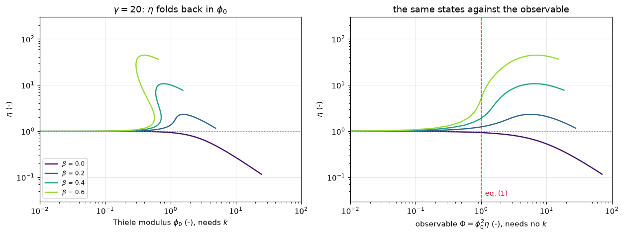
fig, axes = plt.subplots(1, 2, figsize=(11.5, 4.4))
for c, beta in zip(plt.cm.plasma(np.linspace(0.05, 0.7, 3)), (0.2, 0.4, 0.6)):
    br = BR[(beta, 40.0)]
    axes[0].loglog(br.phi, br.eta, color=c, lw=1.6, label=rf"$\beta$ = {beta}")
    axes[1].loglog(br.Phi, br.eta, color=c, lw=1.6,
                   label=rf"$\beta$ = {beta}, fold {FOLD[(beta, 40.0)][1]:.2f}")
axes[0].set_xlabel(r"$\phi_0$ (-)"); axes[1].set_xlabel(r"$\Phi$ (-)")
for a in axes:
    a.set_ylabel(r"$\eta$ (-)"); a.axhline(1.0, color="0.5", lw=0.8, ls=":")
    a.legend(fontsize=8, loc="upper left"); a.set_ylim(0.5, 1e5)
axes[0].set_xlim(1e-3, 3.0)
axes[1].set_xlim(1e-3, 1e2)
axes[1].axvline(1.0, color="crimson", lw=1.0, ls="--")
axes[1].text(1.15, 0.7, "eq. (1)", color="crimson", fontsize=9)
axes[0].set_title(r"$\gamma = 40$")
axes[1].set_title(r"$\Phi$ folds back too: one $\Phi$, three $\eta$")
fig.tight_layout(); plt.show()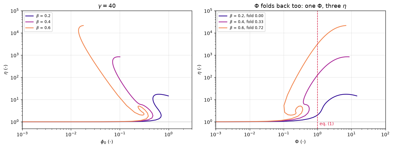
fig, ax = plt.subplots(figsize=(7.2, 4.4))
for c, gamma in zip(plt.cm.viridis(np.linspace(0.05, 0.85, 4)), GAMMAS):
    b = [k[0] for k in MAP if k[1] == gamma]
    e1 = [MAP[(x, gamma)]["eta_iso"] for x in b]
    e2 = [MAP[(x, gamma)]["eta_nis"] for x in b]
    ax.semilogy(b, e1, "o-", color=c, lw=1.5, ms=4, label=rf"eq. (1), $\gamma$ = {gamma:.0f}")
    ax.semilogy([x for x, v in zip(b, e2) if v], [v for v in e2 if v], "s--",
                color=c, lw=1.0, ms=3, alpha=0.7)
ax.axhspan(0.95, 1.05, color="0.85", zorder=0)
ax.set_xlabel(r"Prater number $\beta$ (-)"); ax.set_ylabel(r"$\eta$ at the criterion's threshold (-)")
ax.set_title("What each criterion admits (solid: eq. 1; dashed: eq. 10a)")
ax.legend(fontsize=8, loc="upper left")
ax.set_xlim(-0.48, 0.85)
fig.tight_layout(); plt.show()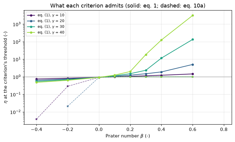
Validation
Tier 6. Nothing on this page is compared with a measurement, and none of what follows is validation against experiment. What is available is a closed form, a second numerical method, and printed numerical statements. Ranked, strongest first:
- The shooting reference against the exact isothermal \(\eta\), three geometries, seven states each, on an integration-tolerance ladder. This is what licenses every branch result, because the branch tracer is the only route to the unstable middle branch.
- pymrm against the same closed form, on a grid ladder, at the observed order of every case.
- pymrm against the shooting solution in the non-isothermal case, over the whole branch including its unstable part, on a grid ladder. The two share only the rate law: one is a finite-volume solve in \(u\), the other an initial-value integration in \(s = \phi_0 u\).
- The threshold two ways: a root scan on pymrm against the closed form; and, for the other kinetics, pymrm on every \(\Phi = 1\) state the shooting branch contains.
- Printed statements reproduced: the worked \(\gamma = 20\), \(\beta = 0.3\) case giving \(\phi_0 \sim 0.1\), the multiplicity onset at \(\beta\gamma \gtrsim 5\), and \(Q'/Q\) between 1 and \(\tfrac12\). None is an input to anything.
Two checks look like evidence and are weaker. The observable computed as the volume average of the rate, \(\phi_0^2\langle\mathcal{R}\rangle\), against the surface flux: construct_div is conservative, so the volume-weighted sum of the residual telescopes to the surface flux and \(\Phi_{\text{flux}} - \Phi_{\text{volume}} = \frac{\nu+1}{V}\sum_i V_i\,\mathrm{res}_i\), the solve residual again. It catches a solve that has not converged and a rate that differs from the one used to interpret it; a wrong geometry index or a coarse grid changes both sides alike. And a converged residual says the equations are solved, not which solution was found: the second cell below starts Newton from \(y = 1\) on a folded branch.
ref = P800["sphere"]
PH_REF = TH["sphere"][0]
y_ref = ref.solve(PH_REF, R1)[0]
R_WH = WeiszHicks(0.3, 20.0)


def flux_vol_gap(pellet, model_rate, interp_rate=R1, maxfev=60):
    ph = PH_REF
    y = pellet.solve(ph, model_rate, maxfev=maxfev, check=maxfev > 1)[0]
    return abs(pellet.Phi(y) - pellet.Phi_from_volume(y, ph, interp_rate))


claims.bound("Phi_flux_minus_Phi_volume",
             max(flux_vol_gap(ref, R1), flux_vol_gap(ref, R_WH, R_WH)),
             max=1e-9, basis="tolerance", note="the volume-weighted residual of a newton solve, tol 1e-12, "
             "first order and the non-isothermal rate beta = 0.3, gamma = 20, both on the sphere at PH_REF")
print(f"first-order and non-isothermal (beta = 0.3, gamma = 20) sphere at the first-order threshold, "
      f"800 cells: Phi(flux) - Phi(volume) below 1e-9 (here {claims['Phi_flux_minus_Phi_volume']:.1e})")


brk("rate 1 % too large in the model (scale=1.01)", "Phi_flux_minus_Phi_volume",
    flux_vol_gap(ref, WeiszHicks(0.0, 20.0, scale=1.01)))
brk("newton stopped after one iteration (maxfev=1)", "Phi_flux_minus_Phi_volume",
    max(flux_vol_gap(ref, R1, maxfev=1), flux_vol_gap(ref, R_WH, R_WH, maxfev=1)))
brk("sphere assembled with nu = 0", "Phi_flux_minus_Phi_volume",
    flux_vol_gap(Pellet("sphere", 800, nu=0), R1))
brk("sphere on 3 cells", "Phi_flux_minus_Phi_volume", flux_vol_gap(Pellet("sphere", 3), R1))
first-order and non-isothermal (beta = 0.3, gamma = 20) sphere at the first-order threshold, 800 cells: Phi(flux) - Phi(volume) below 1e-9 (here 8.5e-12)False# A converged solve on a folded branch: the ignited state of beta = 0.6,
# gamma = 20, seeded from the shooting profile, and the same phi_0 from y = 1.
br_h = BR[(0.6, 20.0)]
tau_h = br_h.tau[np.argmax(br_h.eta)]
hard = Pellet("sphere", 800)
PHI_H, y_seed = br_h.profile(tau_h, hard.u_c)
R_H = WeiszHicks(0.6, 20.0)
ETA_H = shoot(2, R_H, np.exp(tau_h), rtol=1e-11)[1]
def ignited_gap(seed=True):
y = hard.solve(PHI_H, R_H, y_init=y_seed if seed else None)[0]
return abs(hard.eta(y, PHI_H) / ETA_H - 1)
claims.value("ignited_state_eta_pymrm_vs_shooting", ignited_gap(), rtol=1e-3)
brk("newton started from y = 1 instead of the shooting profile", "ignited_state_eta_pymrm_vs_shooting",
ignited_gap(seed=False))
y_cold, sol_cold = hard.solve(PHI_H, R_H)
n_here = (sum(int((a - PHI_H) * (b - PHI_H) < 0) for a, b in zip(br_h.phi[:-1], br_h.phi[1:]))
+ int(np.sum(br_h.phi == PHI_H))) # PHI_H is itself a traced state
print(f"beta = 0.6, gamma = 20, phi_0 = {PHI_H:.5f}: the branch carries {n_here} steady states here.")
print(f" seeded from the shooting profile: eta = {hard.eta(hard.solve(PHI_H, R_H, y_init=y_seed)[0], PHI_H):.5f}"
f" (shooting {ETA_H:.5f})")
print(f" started from y = 1 : eta = {hard.eta(y_cold, PHI_H):.5f}, newton '{sol_cold.message}'"
f" (here {sol_cold.nit} iterations)")
print("Both solves converge; the cold one found another solution of the same equations.")
print("Only the branch trace says which, which is why every multiplicity result here is")
print("located on the shooting branch first.")beta = 0.6, gamma = 20, phi_0 = 0.39677: the branch carries 3 steady states here.
seeded from the shooting profile: eta = 44.55472 (shooting 44.55465)
started from y = 1 : eta = 1.15529, newton 'Converged' (here 4 iterations)
Both solves converge; the cold one found another solution of the same equations.
Only the branch trace says which, which is why every multiplicity result here is
located on the shooting branch first.The break table
Every number above is registered as a claim; each row below injects one defect through an argument or a parameter and reports what the claim becomes, and whether the claim’s own check catches it. Rows that a claim does not catch are kept: they show what that check is blind to.
print(f"{'injected defect':<74} {'claim':<40} {'clean':>11} {'broken':>16}  caught")
for name, metric, clean, broken, caught in BREAK:
    is_bound = claims.metrics[metric]["kind"] == "bound"
    shown = f"(here {clean:.0e})" if is_bound else f"{float(clean):11.4g}"
    print(f"{name[:74]:<74} {metric[:40]:<40} {shown:>11} {'(here %.3g)' % float(broken):>16}  "
          f"{'yes' if caught else 'NO'}")
_caught = {m for _, m, _, _, c in BREAK if c}
_structural = sorted(k for k, c in claims.metrics.items() if c.get("structural"))
_open = sorted(k for k in claims.metrics if k not in _caught and k not in _structural)
print(f"\n{len(BREAK)} rows; {len(_caught)} of {len(claims.metrics)} claims are failed by at "
      f"least one row; structural: {', '.join(_structural) or 'none'}; "
      f"open: {', '.join(_open) or 'none'}")
_uncaught = [(n, m) for n, m, _, _, c in BREAK if not c]
print("rows that do not fail their claim: "
      + ("; ".join(f"{n} -> {m}" for n, m in _uncaught) or "none"))
injected defect claim clean broken caught
Phi read by a two-point gradient from the last cell centre (two_point=True surface_gradient_cbv_vs_operator_row (here 0e+00) (here 0.000701) yes
Jacobian by NumJac differencing (jacobian='numjac') cold_scan_failed_solves_exact_jacobian 13 (here 18) yes
eq. (10) exponent without its 1 + beta (denominator=False) eq10_worked_case_phi0 0.09949 (here 0.0498) yes
shooting integrated at rtol 1e-6 shooting_vs_exact_isothermal_eta (here 8e-11) (here 8.71e-06) yes
Phi read by a two-point gradient from the last cell centre (two_point=True pymrm_vs_exact_isothermal_eta_n400 8.311e-06 (here 0.00617) yes
Phi read by a two-point gradient from the last cell centre (two_point=True pymrm_vs_exact_order_min (here 2e+00) (here 0.967) yes
Phi read by a two-point gradient from the last cell centre (two_point=True pymrm_vs_exact_order_max (here 3e+00) (here 1) yes
sphere assembled with nu = 0 pymrm_vs_exact_isothermal_eta_n400 8.311e-06 (here 0.63) yes
orders read at 1600 cells instead of 200 (finest grid moved up three facto pymrm_vs_exact_finest_over_roundoff_min (here 1e+05) (here 65.5) yes
Phi read by a two-point gradient from the last cell centre (two_point=True pymrm_vs_shooting_nonisothermal_n800 5.016e-05 (here 0.00141) yes
Phi read by a two-point gradient from the last cell centre (two_point=True pymrm_vs_shooting_order_min (here 2e+00) (here 0.955) yes
Phi read by a two-point gradient from the last cell centre (two_point=True pymrm_vs_shooting_order_max (here 2e+00) (here 1.27) yes
orders taken over all 18 states, those near eta = 1 included (no |eta - 1| pymrm_vs_shooting_finest_over_roundoff_m (here 3e+05) (here 1) yes
Phi read by a two-point gradient from the last cell centre (two_point=True pymrm_vs_shooting_excluded_worst_n800 0.9447 (here 0.957) yes
closed form of the slab evaluated with nu = 2 eta_at_Phi1_slab_first_order 0.6948 (here 0.935) yes
closed form of the cylinder evaluated with nu = 2 eta_at_Phi1_cylinder_first_order 0.8805 (here 0.935) yes
closed form of the sphere evaluated with nu = 0 eta_at_Phi1_sphere_first_order 0.9353 (here 0.695) yes
sphere assembled with nu = 0 threshold_eta_pymrm_vs_closed_form 1.113e-07 (here 0.257) yes
sphere on 3 cells threshold_eta_pymrm_vs_closed_form 1.113e-07 (here 0.00818) yes
rate 1 % too large in the model (scale=1.01) threshold_eta_pymrm_vs_closed_form 1.113e-07 (here 0.01) yes
sphere closed form evaluated with nu = 1 eta_at_Phi1_spread_on_R 0.2405 (here 0.186) yes
V/S observable divided by nu + 1 instead of (nu + 1)^2 eta_at_Phi1_spread_on_VS 0.1316 (here 0.123) yes
pymrm pellet assembled with nu = 1 threshold_eta_pymrm_vs_shooting_kinetics (here 2e-07) (here 0.0866) yes
branch traced with nu = 1 eta_at_Phi1_second_order 0.8796 (here 0.788) yes
branch traced with nu = 1 eta_at_Phi1_inhibited_LH 1.048 (here 1.1) yes
branch traced with nu = 1 zero_order_dead_core_Phi 6 (here 4) yes
relation with factor 1 instead of 1/2 q_ratio_at_threshold_sphere 0.9371 (here 0.874) yes
relation with factor 1 instead of 1/2 q_ratio_at_threshold_slab 0.7196 (here 0.439) yes
sphere closed form without its small-phi series (stable=False) one_minus_Q_ratio_at_phi0_1e-3 6.667e-08 (here 9.92e-07) yes
sphere closed form without its small-phi series (stable=False) Q_ratio_monotone_decreasing 1 (here 0) yes
relation with factor 1 instead of 1/2 Q_ratio_at_phi0_1e3 0.5005 (here 0.001) yes
branch traced with nu = 1 at beta = 0.6, gamma = 40 eta_at_Phi1_worst_exothermic 3136 (here 6.24e+03) yes
branch traced with nu = 1 at beta = -0.4, gamma = 40 eta_at_Phi1_worst_endothermic 0.4838 (here 0.314) yes
sign of the exponent flipped (sign=-1) eta_at_Phi1_beta03_gamma20 1.5 (here 0.694) yes
eq. (10a) exponent without its 1 + beta (denominator=False) eq10a_worst_eta_deviation_exothermic 0.01338 (here 0.00903) yes
eq. (10a) exponent without its 1 + beta (denominator=False) eq10a_max_conservatism 1.01e+05 (here 8.18e+08) yes
eq. (10a) exponent without its 1 + beta (denominator=False) eq10a_endothermic_eta_at_threshold_max 0.2898 (here 0.403) yes
eq. (10a) exponent without its 1 + beta (denominator=False) endothermic_cases_beyond_ladder 5 (here 2) yes
eq. (1) threshold read as 0.3 endothermic_beyond_ladder_eta_below_half 1 (here 0) yes
eq. (10a) exponent without its 1 + beta (denominator=False) fn_eq10a_exothermic 0 (here 0) NO
eq. (10a) without its exponential factor (eq. (1) applied) fn_eq10a_exothermic 0 (here 252) yes
eq. (10a) exponent without its 1 + beta (denominator=False) fp_eq10a_exothermic 406 (here 471) yes
truth tolerance 10 % for 5 % not_clean_endothermic 384 (here 343) yes
truth tolerance 10 % for 5 % fn_eq1_exothermic 252 (here 173) yes
truth tolerance 10 % for 5 % fn_eq10a_endothermic 369 (here 328) yes
class read from etas interpolated along the traced ladder fn_eq1_exothermic 252 (here 261) yes
class read from etas interpolated along the traced ladder fp_eq10a_exothermic 406 (here 397) yes
class read from etas interpolated along the traced ladder fn_eq10a_endothermic 369 (here 374) yes
class read from etas interpolated along the traced ladder not_clean_endothermic 384 (here 389) yes
truth tolerance 10 % for 5 % interpolated_class_flips 14 (here 7) yes
branches traced on 12 states instead of 110 (n=12) phi0_multivalued_cases 11 (here 9) yes
branches traced on 12 states instead of 110 (n=12) Phi_multivalued_cases 4 (here 1) yes
turning points read off the traced ladder (refine=False) observable_fold_turning_point_Phi_max 0.8055 (here 0.805) yes
turning points read off the traced ladder (refine=False) observable_fold_depth_worst 0.7272 (here 0.721) yes
eq. (1) threshold read as 0.3 Phi1_unique_root_cases 32 (here 31) yes
branches traced on 12 states instead of 110 (n=12) ambiguous_measurements 14 (here 4) yes
branches traced on 12 states instead of 110 (n=12) ambiguous_measurement_Phi_max 0.5623 (here 0.237) yes
etas interpolated along the traced ladder, not root-found ambiguous_measurement_worst_eta_min 2.186 (here 2.28) yes
etas interpolated along the traced ladder, not root-found ambiguous_measurement_worst_eta_spread 100.7 (here 99.2) yes
exponent without its 1 + beta (1 - y) (denominator=False), gamma = 40 multiplicity_onset_betagamma_min 4.911 (here 4.4) yes
exponent without its 1 + beta (1 - y) (denominator=False), gamma = 20 multiplicity_onset_betagamma_max 5.565 (here 4.4) yes
exponent without its 1 + beta (1 - y) (denominator=False), gamma = 40 observable_fold_onset_betagamma_min 10.84 (here 7.75) yes
exponent without its 1 + beta (1 - y) (denominator=False), gamma = 20 observable_fold_onset_betagamma_max 21.74 (here 7.75) yes
largest beta drawn at gamma = 30 read as 0.45 for 0.4 fig7_panels_with_folded_curve 1 (here 2) yes
turning points read off the traced ladder (refine=False) fig7d_fold_width_decades_beta03_gamma40 0.01942 (here 0.0188) yes
turning points read off the traced ladder (refine=False) fig7d_fold_width_px_at_600dpi 6.949 (here 6.72) yes
turning points read off the traced ladder (refine=False) fig7d_fold_in_line_widths 1.158 (here 1.12) yes
rate 1 % too large in the model (scale=1.01) Phi_flux_minus_Phi_volume (here 8e-12) (here 0.00999) yes
newton stopped after one iteration (maxfev=1) Phi_flux_minus_Phi_volume (here 8e-12) (here 0.456) yes
sphere assembled with nu = 0 Phi_flux_minus_Phi_volume (here 8e-12) (here 1.04e-11) NO
sphere on 3 cells Phi_flux_minus_Phi_volume (here 8e-12) (here 7.66e-15) NO
newton started from y = 1 instead of the shooting profile ignited_state_eta_pymrm_vs_shooting 1.664e-06 (here 0.974) yes
72 rows; 61 of 62 claims are failed by at least one row; structural: eta_at_Phi1_zero_order_dev; open: none
rows that do not fail their claim: eq. (10a) exponent without its 1 + beta (denominator=False) -> fn_eq10a_exothermic; sphere assembled with nu = 0 -> Phi_flux_minus_Phi_volume; sphere on 3 cells -> Phi_flux_minus_Phi_volumeWhat pymrm adds
Nothing to the criterion, which is one line of algebra, and nothing to Weisz and Hicks’ extension of it; both are reproduced as printed. What the page adds is the part the sources leave as an order of magnitude, computed with two independent solvers that agree to the levels printed above. pymrm supplies one of them: the finite-volume pellet with operators assembled once, an exact Jacobian through construct_coefficient_matrix, newton with bounds, the surface gradient through compute_boundary_values, and the root scans of pymrm.checks.find_roots. The other, the shooting branch tracer, uses SciPy integration and a generic root scan (find_roots), independent of pymrm’s discretisation, and it carries every multiplicity result; pymrm’s role there is to confirm the traced states on a grid.
display(Markdown(f"""
- **The threshold's guarantee, as a number.** $\\Phi < 1$ admits
  $\\eta = {claims['eta_at_Phi1_sphere_first_order']:.4f}$ for a first-order sphere and
  ${claims['eta_at_Phi1_slab_first_order']:.4f}$ for a slab. Measured on the
  volume-to-surface length instead, the spread across geometries falls from
  ${claims['eta_at_Phi1_spread_on_R']:.3f}$ to ${claims['eta_at_Phi1_spread_on_VS']:.3f}$.
  Across kinetics on one shape the guarantee runs from exactly 1 (zero order)
  through ${claims['eta_at_Phi1_second_order']:.4f}$ (second order) to
  ${claims['eta_at_Phi1_inhibited_LH']:.4f}$ for a self-inhibited Langmuir-Hinshelwood
  rate, above 1 with no heat effect.
- **Where the isothermal form fails, quantified.** For an exothermic pellet eq. (1)
  admits $\\eta$ up to ${claims['eta_at_Phi1_worst_exothermic']:.4g}$. Eq. (10a) passes
  {claims['fn_eq10a_exothermic']} of the unclean measurements here and holds $\\eta$ within
  ${100 * claims['eq10a_worst_eta_deviation_exothermic']:.1f}$ % of 1 at its threshold, paying
  with a conservatism up to a factor ${claims['eq10a_max_conservatism']:.3g}$ in $\\Phi$.
- **The endothermic case, where the extension inverts.** Its threshold exceeds 1;
  it is reached only at $\\eta \\le {claims['eq10a_endothermic_eta_at_threshold_max']:.3g}$,
  so eq. (10a) passes {claims['fn_eq10a_endothermic']} of the
  {claims['not_clean_endothermic']} unclean endothermic measurements.
- **A quantitative limit on the Section V claim.** The observable postpones the
  multiplicity, from $\\beta\\gamma = {claims['multiplicity_onset_betagamma_min']:.2f}$ to
  ${claims['multiplicity_onset_betagamma_max']:.2f}$ in $\\phi_0$ to
  ${claims['observable_fold_onset_betagamma_min']:.2f}$ to
  ${claims['observable_fold_onset_betagamma_max']:.2f}$ in $\\Phi$; $\\Phi$ is multivalued in
  {claims['Phi_multivalued_cases']} of the 32 swept cases, inside the range the paper
  says it computed.
- **Every fold sits below $\\Phi = 1$** (largest turning point
  ${claims['observable_fold_turning_point_Phi_max']:.4f}$), inside the band the criterion
  certifies as safe; $\\Phi = 1$ keeps a unique root in {claims['Phi1_unique_root_cases']} of 32.
  {claims['ambiguous_measurements']} measurements on this page's grid fit more than one state, the
  worst with an $\\eta$ spread of a factor ${claims['ambiguous_measurement_worst_eta_spread']:.1f}$.
- **What Fig. 7 can settle, in pixels.** {claims['fig7_panels_with_folded_curve']} of its four
  panels draws a curve in the folded regime; that fold spans
  ${claims['fig7d_fold_width_px_at_600dpi']:.1f}$ px at 600 dpi against a 6 to 7 px stroke, so the
  figure is silent. A limit on the claim, not a refutation: the criterion works
  everywhere the authors apply it.
"""))- The threshold’s guarantee, as a number. \(\Phi < 1\) admits \(\eta = 0.9353\) for a first-order sphere and \(0.6948\) for a slab. Measured on the volume-to-surface length instead, the spread across geometries falls from \(0.240\) to \(0.132\). Across kinetics on one shape the guarantee runs from exactly 1 (zero order) through \(0.8796\) (second order) to \(1.0483\) for a self-inhibited Langmuir-Hinshelwood rate, above 1 with no heat effect.
- Where the isothermal form fails, quantified. For an exothermic pellet eq. (1) admits \(\eta\) up to \(3136\). Eq. (10a) passes 0 of the unclean measurements here and holds \(\eta\) within \(1.3\) % of 1 at its threshold, paying with a conservatism up to a factor \(1.01e+05\) in \(\Phi\).
- The endothermic case, where the extension inverts. Its threshold exceeds 1; it is reached only at \(\eta \le 0.29\), so eq. (10a) passes 369 of the 384 unclean endothermic measurements.
- A quantitative limit on the Section V claim. The observable postpones the multiplicity, from \(\beta\gamma = 4.91\) to \(5.56\) in \(\phi_0\) to \(10.84\) to \(21.74\) in \(\Phi\); \(\Phi\) is multivalued in 4 of the 32 swept cases, inside the range the paper says it computed.
- Every fold sits below \(\Phi = 1\) (largest turning point \(0.8055\)), inside the band the criterion certifies as safe; \(\Phi = 1\) keeps a unique root in 32 of 32. 14 measurements on this page’s grid fit more than one state, the worst with an \(\eta\) spread of a factor \(100.7\).
- What Fig. 7 can settle, in pixels. 1 of its four panels draws a curve in the folded regime; that fold spans \(6.9\) px at 600 dpi against a 6 to 7 px stroke, so the figure is silent. A limit on the claim, not a refutation: the criterion works everywhere the authors apply it.
Reuse
| Change | Where |
|---|---|
| Different geometry | Pellet(geom=...), or a callable nu in construct_div |
| Different kinetics | any object with r(y) and dr(y); jacobian="numjac" if dr is not available |
| Your own measurement | Branch(nu, rate).all_where(lambda p, e, P: P - your_Phi): the inversion needs no \(k\), and it returns every consistent state |
| Non-isothermal | WeiszHicks(beta, gamma), the reduced eq. (9) |
| Two fields instead of one | B1.6’s two-field pellet, if you do not want the Prater relation substituted |
| The unstable branch | Branch, parametrised by \(y_c\), not \(\phi_0\); Branch.profile seeds Pellet.solve there |
How to use the criterion, given what is above. Compute \(\Phi = r_{\mathrm{obs}}L^2/(D_ec_s)\) and state the length scale: the threshold and the length are not separable, and quoting \(\Phi < 1\) without saying whether \(L\) is \(R\) or \(V/S\) leaves a factor \((\nu+1)^2 = 9\) on a sphere. If the reaction is exothermic, estimate \(\beta\) and \(\gamma\) and use eq. (10a), not eq. (1). If \(\beta\gamma\) is above the onsets printed in the fold section, the observable may no longer determine the state. And a passing \(\Phi\) still admits several per cent in \(\eta\) and in the apparent activation energy; the threshold section prints both, per geometry.
Reading Weisz and Hicks. The scan’s text layer is unusable for equations. Render the journal page at 600 dpi and read it. Same trap as B3.1 and B1.6, recorded in docs/pdf-findings.md.
Related pages. B1.1/B1.5, the forward problem \(\eta(\phi_0)\) and the multiplicity this page views through the observable; B1.6, the Prater relation that reduces the two balances to the one equation used here; B1.2 Aris generalised modulus and B1.3 Bischoff generalised modulus, the length-scale question; B1.7 Mears criteria, the same observable-only logic for external gradients.
References
Weisz, P. B. and Prater, C. D. (1954). In Advances in Catalysis, Vol. 6, p. 143. Academic Press, New York. The origin the criterion is named for; not consulted, no copy on disk and no open-access route. Given as Weisz and Hicks’ reference [5] prints it on journal page 274, with no chapter title.
Weisz, P. B. (1957). Z. Phys. Chem. 11, 1. The reference Weisz and Hicks attach to eq. (1). Not consulted.
Weisz, P. B. and Hicks, J. S. (1962). The behaviour of porous catalyst particles in view of internal mass and heat diffusion effects. Chemical Engineering Science 17(4), 265-275. doi:10.1016/0009-2509(62)85005-2. The source actually read: eqs. (1), (9), (10), (10a) and (11), the \(Q'/Q\) relation, the \(\beta\gamma \gtrsim 5\) statement and the Section V claim from 600 dpi renders of journal pages 265, 267, 268, 269, 272 and 273; the two references above from page 274; the Fig. 7(d) axis calibration and stroke width from the render of page 272.
# Claims: prints every registered number, writes agreement.json for CI, and
# raises when a claim fails its own check or has no break row.
claims.report();   # the semicolon keeps the notebook from echoing the payload
Claims for B1.4:
surface_gradient_cbv_vs_operator_row = (here 0.0e+00) bound bound <= 1e-12 [identity]
cold_scan_failed_solves_exact_jacobian = 13 exact exact
eq10_worked_case_phi0 = 0.099491 value rtol 1e-06
shooting_vs_exact_isothermal_eta = (here 8.4e-11) bound bound <= 1e-09 [tolerance]
pymrm_vs_exact_isothermal_eta_n400 = 8.3106e-06 value rtol 0.001
pymrm_vs_exact_order_min = (here 2.0e+00) bound bound [1.9, 3.1] [chosen]
pymrm_vs_exact_order_max = (here 3.0e+00) bound bound [1.9, 3.1] [chosen]
pymrm_vs_exact_finest_over_roundoff_min = (here 1.0e+05) bound bound >= 1000 [theory]
pymrm_vs_shooting_nonisothermal_n800 = 5.0157e-05 value rtol 0.001
pymrm_vs_shooting_order_min = (here 2.0e+00) bound bound [1.9, 2.1] [theory]
pymrm_vs_shooting_order_max = (here 2.0e+00) bound bound [1.9, 2.1] [theory]
pymrm_vs_shooting_finest_over_roundoff_min = (here 3.0e+05) bound bound >= 1000 [theory]
pymrm_vs_shooting_excluded_worst_n800 = 0.94466 value rtol 0.001
threshold_eta_pymrm_vs_closed_form = 1.1127e-07 value rtol 0.05
eta_at_Phi1_slab_first_order = 0.69482 value rtol 1e-06
eta_at_Phi1_cylinder_first_order = 0.88052 value rtol 1e-06
eta_at_Phi1_sphere_first_order = 0.93528 value rtol 1e-06
eta_at_Phi1_spread_on_R = 0.24046 value rtol 1e-06
eta_at_Phi1_spread_on_VS = 0.13156 value rtol 1e-06
threshold_eta_pymrm_vs_shooting_kinetics = (here 2.0e-07) bound bound <= 1e-06 [chosen]
eta_at_Phi1_second_order = 0.87961 value rtol 1e-06
eta_at_Phi1_inhibited_LH = 1.0483 value rtol 1e-06
eta_at_Phi1_zero_order_dev = (here 2.9e-15) bound bound <= 1e-08 [identity]
zero_order_dead_core_Phi = 6 value rtol 1e-06
q_ratio_at_threshold_sphere = 0.93713 value rtol 1e-06
q_ratio_at_threshold_slab = 0.71961 value rtol 1e-06
one_minus_Q_ratio_at_phi0_1e-3 = 6.6667e-08 value rtol 0.0001
Q_ratio_at_phi0_1e3 = 0.5005 value rtol 1e-06
Q_ratio_monotone_decreasing = True exact exact
eta_at_Phi1_worst_exothermic = 3136 value rtol 0.001
eta_at_Phi1_worst_endothermic = 0.48384 value rtol 0.0001
eta_at_Phi1_beta03_gamma20 = 1.4996 value rtol 1e-06
eq10a_worst_eta_deviation_exothermic = 0.013378 value rtol 0.001
eq10a_max_conservatism = 1.0101e+05 value rtol 0.001
eq10a_endothermic_eta_at_threshold_max = 0.28985 value rtol 0.0001
endothermic_cases_beyond_ladder = 5 exact exact
endothermic_beyond_ladder_eta_below_half = 1 exact exact, margin 0.0323
fn_eq1_exothermic = 252 exact exact, margin 3.03e-05
fn_eq10a_exothermic = 0 exact exact, margin 3.03e-05
fp_eq10a_exothermic = 406 exact exact, margin 3.03e-05
fn_eq10a_endothermic = 369 exact exact, margin 0.000789
not_clean_endothermic = 384 exact exact, margin 0.000789
interpolated_class_flips = 14 exact exact, margin 3.03e-05
phi0_multivalued_cases = 11 exact exact, margin 1
Phi_multivalued_cases = 4 exact exact, margin 1
observable_fold_turning_point_Phi_max = 0.8055 value rtol 0.0001
observable_fold_depth_worst = 0.72721 value rtol 0.0001
Phi1_unique_root_cases = 32 exact exact
ambiguous_measurements = 14 exact exact
ambiguous_measurement_Phi_max = 0.56234 value rtol 1e-09
ambiguous_measurement_worst_eta_spread = 100.72 value rtol 0.0001
ambiguous_measurement_worst_eta_min = 2.1855 value rtol 0.001
multiplicity_onset_betagamma_min = 4.9115 value rtol 0.0001
multiplicity_onset_betagamma_max = 5.5645 value rtol 0.0001
observable_fold_onset_betagamma_min = 10.842 value rtol 0.0001
observable_fold_onset_betagamma_max = 21.737 value rtol 0.0001
fig7_panels_with_folded_curve = 1 exact exact, margin 0.0319
fig7d_fold_width_decades_beta03_gamma40 = 0.019416 value rtol 0.0001
fig7d_fold_width_px_at_600dpi = 6.9494 value rtol 0.0001
fig7d_fold_in_line_widths = 1.1582 value rtol 0.0001
Phi_flux_minus_Phi_volume = (here 8.5e-12) bound bound <= 1e-09 [tolerance]
ignited_state_eta_pymrm_vs_shooting = 1.6638e-06 value rtol 0.001