# Bootstrap: the pymrm this page was checked with, and the gallery files it was
# published with. Works in a checkout, in CI and on a fresh Colab VM.
GALLERY_REF = "gallery-2026.11.10.3"  # replaced by the release tag at publication
PYMRM = ">=3.3.0,<4"  # equals meta.yaml pymrm_min_version, up to the next major
PAGE = "B1.6-prater-relation"  # equals the page directory

import os, sys, urllib.request
from pathlib import Path
_shared = next((p / "shared" for p in (Path.cwd(), *Path.cwd().parents)
                if (p / "shared" / "gallery_bootstrap.py").is_file()), None)
if _shared is None:
    _shared = (Path(os.environ.get("XDG_CACHE_HOME") or Path.home() / ".cache")
               / "pymrm-gallery" / GALLERY_REF)
    _shared.mkdir(parents=True, exist_ok=True)
    urllib.request.urlretrieve(
        "https://raw.githubusercontent.com/computational-chemical-engineering/"
        f"pymrm-gallery/{GALLERY_REF}/shared/gallery_bootstrap.py",
        _shared / "gallery_bootstrap.py")
sys.path.insert(0, str(_shared))
sys.modules.pop("gallery_bootstrap", None)
from gallery_bootstrap import setup
setup(PAGE, PYMRM, GALLERY_REF); # the semicolon stops the cell echoing the pathThe Prater relation: a pellet’s temperature is slaved to its concentration
sec:B
struct:S3
tier:T0
data:tier6
phase:gas-solid
One linear identity fixes the temperature everywhere inside a catalyst particle from the concentration alone, whatever the kinetics and whatever the shape. Proved symbolically, confirmed numerically on two-field solves, measured against deliberately injected defects to establish what that confirmation is worth, and then broken on purpose: an external film and a transient with Le different from 1.
The Prater relation: a pellet’s temperature is slaved to its concentration
Catalog ID: B1.6 · Structures: S3 (1D steady BVP) · Tier: T0
Inside a working catalyst particle, reactant is consumed and heat is released at the same points, in fixed proportion. Prater showed in 1958 that this makes the temperature field a linear function of the concentration field, not approximately and not only for a sphere:
\[\lambda\,(T - T_s) \;=\; (-\Delta H)\,D_e\,(c_s - c).\]
No rate constant appears, no activation energy, no particle shape. Solve the diffusion problem and the temperature comes free.
This page proves that, confirms it numerically in pymrm across three geometries and three rate laws, establishes what that numerical confirmation is and is not sensitive to by injecting defects on purpose, and then does the part the 1958 result could not: finds where it stops being true, and by how much.
import numpy as np
import sympy as sp
import matplotlib.pyplot as plt
from scipy.integrate import solve_ivp
from IPython.display import Markdown, display
from pymrm import newton
from gallery_utils import Claims, load_claims
from model import (NU, FirstOrder, LangmuirHinshelwood, ZeroOrder,  # this page's model.py
                   TwoFieldPellet, violation, march, march_ivp, _rhs, peak_of, ReducedPellet,
                   collocation, shooting, shooting_at_phi, prater_beta)

plt.rcParams.update({"figure.dpi": 110, "axes.grid": True, "grid.alpha": 0.3})
np.seterr(over="ignore", under="ignore")   # exp() of a depleted, ignited centre underflows
claims = Claims(PAGE.split("-")[0])
EPS = np.finfo(float).eps
BREAK = []


def brk(row, metric, broken):
    """One injected defect: ``broken`` is what claim ``metric`` becomes with it."""
    caught = claims.breaks(row, metric, broken)
    BREAK.append((row, metric, claims[metric], broken, caught))
    return caught


def ro(x):
    """A round-off-sized number, printed as this run's value."""
    return f"(here {x:.1e})"


def ladder_cell(err, n):
    """A ladder entry; within 1e3 of the round-off estimate n^2 eps its last digits
    are noise, so it is printed as this run's value."""
    return f"{ro(err):>16}" if err < 1e3 * n**2 * EPS else f"{err:16.3e}"
Background
A porous catalyst pellet running an exothermic reaction is governed by two balances that share one source term. Species is consumed at the local rate \(r\); heat is produced at \((-\Delta H)\,r\) at exactly the same place. The two fields are therefore not independent, and Prater’s observation is that they are not even approximately independent: one determines the other exactly.
The practical consequence is the reason every non-isothermal pellet analysis since is a one-variable problem. Weisz and Hicks (1962) say so in as many words: the relation “enables us to write the reaction rate (6) in terms of one variable instead of both, \(c\) and \(\Delta T\)”. Their whole paper, and the B1.1/B1.5 page’s large effectiveness factors and coexisting steady states, rest on it.
It also gives the single most useful number in non-isothermal catalysis for free. Setting \(c \to 0\), a fully diffusion-starved centre, bounds the internal temperature rise:
\[(\Delta T)_{\max} = \frac{(-\Delta H)\,D_e\,c_s}{\lambda},\]
which needs no kinetics at all, only transport properties and the surface concentration. Divided by \(T_s\) it is the Prater number \(\beta\), the parameter labelling the curves on the Weisz-Hicks diagram.
Why does an identity deserve a gallery page? Because it is an unusually clean example of an internal identity the model must satisfy, and because its assumptions are usually left unstated. This page states them, and then breaks each one on purpose.
The published model
Provenance: what was read, and what was not
Prater’s own 1958 paper is not on disk and has no open-access route. It is cited here as the origin of the result, from Weisz and Hicks’ own reference list, which reads:
[11] PRATER C. D., Chem. Engng. Sci. 1958 8 284.
Everything transcribed below comes instead from Weisz and Hicks (1962), which is on disk and is also the source of the published B1.1/B1.5 page. They print the relation as their eq. (7) and attribute it explicitly: Damköhler had it for the sphere, and “this relationship was proven by PRATER [11] to apply to any particle geometry.”
So: the equations on this page are Weisz and Hicks as printed; the result is Prater’s. Nothing here is restated from memory or from a textbook. The scan’s text layer is badly mangled (it renders eq. (7) as AT = T - To = - F / [grad ~1,~~), so every symbol below was read off a 600 dpi render of journal page 266 (pdftoppm -r 600 -f 2 -l 2 -png).
The equations, as printed
Weisz and Hicks define \(K\) = thermal conductivity, \(H\) = molar heat of reaction, and \(\mathrm{d}n/\mathrm{d}t\) = “the actual per unit volume reaction rate in a volume element”. Their transport equations are
\[D\nabla^2 c - \frac{\mathrm{d}n}{\mathrm{d}t} = 0 \tag{4}\]
\[K\nabla^2 T - H\frac{\mathrm{d}n}{\mathrm{d}t} = 0 \tag{5}\]
and the relation itself, printed exactly as
\[\Delta T = T - T_0 = -\frac{HD}{K}\,(c_0 - c), \tag{7}\]
“with \(T_0\) and \(c_0\) being the boundary values”. The dimensionless groups follow as
\[\gamma = \frac{Q}{RT_0}, \qquad \beta = \frac{c_0 H D}{K T_0} = \left(\frac{\Delta T}{T_0}\right)_{\!\max}, \qquad y = \frac{c}{c_0}. \tag{8}\]
One sign has to be resolved before anything is built
Eq. (7) is exactly what eqs. (4) and (5) give; the check below confirms it symbolically. But eq. (7) at \(c \to 0\) gives \((\Delta T/T_0)_{\max} = -c_0HD/(KT_0)\), which is the negative of the middle member of eq. (8). The two printed expressions for \(\beta\) therefore disagree in sign, and the disagreement is not cosmetic: it decides whether an exothermic pellet is hotter or colder inside.
Three pieces of the paper’s own content settle it, and all three agree:
- Eq. (8)’s rate, \(\mathrm{d}n/\mathrm{d}t = k_0c_0\,y\exp\{\gamma\beta(1-y)/[1+\beta(1-y)]\}\), is eq. (6) with \(\Delta T/T_0\) replaced by \(\beta(1-y)\). That substitution requires \(\beta = +(\Delta T/T_0)_{\max}\), the right-hand member.
- The paper sweeps “\(\beta\) in the range from 0 to \(+0.8\) (exothermic reaction) and 0 to \(-0.8\) (endothermic)”.
- Its central result is \(\eta \gg 1\), which needs the exponent to be positive where the pellet is depleted, i.e. hotter inside.
So \(H\) in eqs. (5) and (7) is the molar enthalpy of reaction, negative when heat is released, and \(\beta\) is defined positive for an exothermic reaction. In modern notation, with \((-\Delta H) > 0\) exothermic, \(\lambda\) the effective conductivity and \(D_e\) the effective diffusivity, the two printed statements become unambiguous and are what this page uses throughout:
\[\boxed{\;\lambda\,(T - T_s) = (-\Delta H)\,D_e\,(c_s - c)\;} \qquad \beta = \frac{(-\Delta H)\,D_e\,c_s}{\lambda\,T_s} = \left(\frac{\Delta T}{T_s}\right)_{\!\max}.\]
This is the same \(\beta\) that labels the curves on B1.1/B1.5; the cross-check below confirms the two pages use it identically.
Parameters and assumptions
The relation holds under five assumptions, and this page tests each of them:
| # | assumption | what happens without it |
|---|---|---|
| 1 | steady state | fails; quantified below, exactly recovered when \(Le = 1\) |
| 2 | one reaction, so both balances share one \(r\) | fails (not tested here) |
| 3 | constant \(D_e\) and \(\lambda\) | the linear relation between \(T\) and \(c\) fails. If \(D_e = D_e(c)\) and \(\lambda = \lambda(T)\), the Kirchhoff potentials \(\Phi_c = \int D_e\,\mathrm{d}c\) and \(\Phi_T = \int \lambda\,\mathrm{d}T\) satisfy \(\nabla^2[\Phi_T + (-\Delta H)\Phi_c] = 0\), so what survives is a linear relation between the potentials; between \(T\) and \(c\) it becomes nonlinear (not tested here) |
| 4 | the same boundary condition type for both fields | fails; quantified below |
| 5 | nothing about the kinetics, and nothing about the geometry | these are the point: they are not assumptions |
Everything on this page is dimensionless. With \(u\) the position scaled on the characteristic length \(L\), \(y = c/c_s\) and \(\theta = T/T_s\), the steady pellet is
\[\nabla^2 y = \phi^2\,\mathcal{R}(y,\theta), \qquad \nabla^2 \theta = -\beta\,\phi^2\,\mathcal{R}(y,\theta),\]
with \(\phi = L\sqrt{k_s/D_e}\) the Thiele modulus, \(\gamma = E/(R_gT_s)\) the Arrhenius number, \(\beta\) the Prater number, and \(\nabla^2\) carrying the geometry index \(\nu = 0, 1, 2\) for slab, cylinder and sphere. The two equations are solved as two coupled fields and the Prater relation is never substituted anywhere in the solver; that is the whole design of the page.
Three rate laws are used, all pointwise in \((y,\theta)\):
\[\mathcal{R}_{1} = y\,e^{\gamma(1-1/\theta)}, \qquad \mathcal{R}_{\mathrm{LH}} = \frac{y\,e^{\gamma(1-1/\theta)}}{\left[1 + K(\theta)\,y\right]^2}, \quad K(\theta) = K_s e^{\gamma_a(1/\theta-1)}, \qquad \mathcal{R}_{0} = e^{\gamma(1-1/\theta)} .\]
\(\mathcal{R}_1\) is Weisz and Hicks’ own kinetics written in \(\theta\); the other two are chosen because the identity claims they cannot matter. The Langmuir-Hinshelwood form carries a second temperature dependence, in the adsorption constant (\(\gamma_a = 8\), \(K_s = 3\)), which is the sharpest available test of that claim.
# The sweep: every case is solved as two fields on N_SWEEP cells.
KIN = {"first order": FirstOrder, "Langmuir-Hinshelwood": LangmuirHinshelwood,
       "zero order": ZeroOrder}
SWEEP = [("first order",          (0.3, 1.0, 2.0), (-0.4, -0.1, 0.1, 0.3, 0.6)),
         ("Langmuir-Hinshelwood", (0.3, 1.0, 2.0), (-0.4, -0.1, 0.1, 0.3, 0.6)),
         ("zero order",           (0.2, 0.4),      (-0.4, -0.1, 0.1))]   # (kinetics, phi, beta)
GAMMAS = (10.0, 20.0, 30.0)        # Arrhenius numbers [-]
N_SWEEP = 200                      # cells [-]
CASES = [(kin, geom, gamma, beta, phi) for kin, phis, betas in SWEEP for geom in NU
         for gamma in GAMMAS for beta in betas for phi in phis]
print(f"{len(CASES)} cases: 3 geometries, 3 rate laws, {len(GAMMAS)} Arrhenius numbers, "
      f"Prater numbers from {min(min(b) for _, _, b in SWEEP)} to {max(max(b) for _, _, b in SWEEP)}")
324 cases: 3 geometries, 3 rate laws, 3 Arrhenius numbers, Prater numbers from -0.4 to 0.6The data
There is none, and there does not need to be: provenance tier 6.
This page compares a model with an identity, not with a measurement. Weisz and Hicks (1962) report no experimental data at all (the same finding recorded for B1.1), and Prater (1958) is a theoretical note. The validation route used here, an internal identity the model must satisfy, needs no dataset and no digitised figure. Nothing on this page is digitised and no CSV is shipped.
This is a proof plus numerical confirmation. It is not experimental validation, and the two must not be blurred. A pellet whose measured centre temperature matched \(\beta T_s(1-y_c)\) would be validation; nothing below is.
PyMRM implementation
TwoFieldPellet in model.py discretises the two balances as an honest coupled system and lets the solver find both fields; nowhere does it use \(\theta = 1 + \beta(1-y)\).
- One state, two fields, spatial axis first.
BlockLayout.from_fields(["y", "theta"], (n,))gives the(n, 2)state,yin column 0 andthetain column 1; oneconstruct_gradand oneconstruct_divon that shape serve both fields. The operatordiv gradis assembled once per pellet. - Boundary conditions use the OUTWARD normal, one column per field. At the centre the outward normal points inward, so symmetry is \(\partial y/\partial n
= 0\); at the surface it points outward, so a film reads \(\partial y/\partial n + Bi\,y = Bi\) with the same sign for both fields. Each
bcinmodel.pycarries its physical equation in a comment. - The exact Jacobian. The rate couples \(y\) and \(\theta\) at the same point only, so its Jacobian is one 2 x 2 block per cell,
construct_coefficient_matrix(dsrc, shape=((n, 2, 1), (n, 1, 2)))withdsrc[i, a, b]the derivative of sourceawith respect to fieldb, added to the constantdiv grad. - The solve.
pseudo_transientfrom the surface state \(y = \theta = 1\): a steady Newton solve first, which is all most cases need, and where that fails, implicit pseudo-time steps with equal capacities for both fields (a start-up at \(Le = 1\) in those cases), finished by a steadynewtonwithtol=1e-12andstagnation=True. The solve raises unless that Newton solve reports success. A march needs no path in \(\beta\), so it cannot stop at a fold on the way to the case it solves. Where several steady states exist, the solve lands on the least-ignited one, the state a start-up from surface conditions reaches; the cell after the cross-page checks counts those cases and checks one of them against a resolved \(Le = 1\) start-up.boundskeeps \(\theta\) above 0.2 during the iteration. That floor is a numerical safeguard: the Arrhenius factors stay finite down to about 0.012, and by the Prater identity every root has \(\theta \ge 1 + \beta_{\min}\) (printed under the sweep), so the floor cannot bind at a root; the solve checks that no converged state comes near it.
Surface values and the surface flux are read with compute_boundary_values, so the effectiveness factor is the flux the operator transports.
_pel = TwoFieldPellet("sphere", 4)
print("state shape", _pel.shape, "fields", list(_pel.layout.shapes), "; div grad nonzeros:",
      _pel.lap.nnz, "(two tridiagonal blocks, interleaved)")
state shape (4, 2) fields ['y', 'theta'] ; div grad nonzeros: 20 (two tridiagonal blocks, interleaved)Results
1. The proof, in one line
Multiply the species balance by \(\beta\) and add the energy balance. The rate cancels identically, whatever function it is, leaving
\[\nabla^2\!\left(\theta + \beta y\right) = 0 .\]
So \(w = \theta + \beta y\) is harmonic. It equals \(1+\beta\) on the whole boundary, because both fields are Dirichlet there with the same reference values. A harmonic function equal to a constant on the boundary of a bounded domain equals that constant everywhere (uniqueness of the Dirichlet problem, or the maximum principle), and that argument uses nothing about the shape of the domain, which is exactly Prater’s claim about “any particle geometry”. Hence \(\theta + \beta y \equiv 1 + \beta\), which is the relation.
The cell below does this symbolically for a general geometry index \(\nu\) and a completely unspecified rate function.
u = sp.Symbol("u", positive=True)
nu_s, beta_s, phi_s, gamma_s = sp.symbols("nu beta phi gamma", real=True)
y_f, th_f, w_f = sp.Function("y"), sp.Function("theta"), sp.Function("w")
R_f = sp.Function("R")            # completely arbitrary kinetics


def laplacian(f):
    """(1/u^nu) d/du (u^nu df/du): slab, cylinder, sphere and everything between."""
    return sp.diff(f, u, 2) + nu_s * sp.diff(f, u) / u


def rate_cancels(species_sign=-1):
    """Whether energy + beta*species - laplacian(theta + beta*y) vanishes for any R.
    ``species_sign=+1`` writes the species balance with the source's sign flipped."""
    rate_sym = R_f(y_f(u), th_f(u))
    res_species = laplacian(y_f(u)) + species_sign * phi_s**2 * rate_sym   # = 0
    res_energy = laplacian(th_f(u)) + beta_s * phi_s**2 * rate_sym        # = 0
    combo = sp.simplify(res_energy + beta_s * res_species - laplacian(th_f(u) + beta_s * y_f(u)))
    return combo == 0, combo


IDENTITY_OK, _combo = rate_cancels()
print("energy + beta*species - laplacian(theta + beta*y)  =", _combo)
claims.exact("identity_symbolic", bool(IDENTITY_OK))

# a harmonic function with a symmetric centre is constant. dsolve's general form
# degenerates at nu = 1 (the cylinder), where the second solution is log u.
gen = sp.dsolve(sp.Eq(laplacian(w_f(u)), 0), w_f(u)).rhs
print("general solution of laplacian(w) = 0, generic nu :", sp.simplify(gen))
for nu_val in (0, 1, 2):
    g_i = sp.dsolve(sp.Eq(laplacian(w_f(u)).subs(nu_s, nu_val), 0), w_f(u)).rhs
    print(f"   nu = {nu_val} ({['slab', 'cylinder', 'sphere'][nu_val]:8s})"
          f"                       : {sp.simplify(g_i)}")
print("The second solution is singular at the centre for nu >= 1 (log u at nu = 1,")
print("u^(1-nu) for nu > 1) and has non-zero slope there for nu = 0, so regularity")
print("plus dw/du(0) = 0 leaves only the constant: theta + beta*y = 1 + beta")
print("everywhere, for any R and any nu.")
energy + beta*species - laplacian(theta + beta*y) = 0
general solution of laplacian(w) = 0, generic nu : C1 + C2*u**(1 - nu)
nu = 0 (slab ) : C1 + C2*u
nu = 1 (cylinder) : C1 + C2*log(u)
nu = 2 (sphere ) : C1 + C2/u
The second solution is singular at the centre for nu >= 1 (log u at nu = 1,
u^(1-nu) for nu > 1) and has non-zero slope there for nu = 0, so regularity
plus dw/du(0) = 0 leaves only the constant: theta + beta*y = 1 + beta
everywhere, for any R and any nu.2. Checking the transcription before building on it
A reading off a page image is a transcription and needs checking like any other. Three checks, all using only the paper’s own printed content.
D, K, H, c0, T0, c, T, lap_c, lap_T, dndt = sp.symbols("D K H c_0 T_0 c T L_c L_T n", real=True)
y_s = sp.Symbol("y", positive=True)
x_s = sp.Symbol("x", real=True)


def transcription(h_sign=1, eq8_denominator_sign=1):
    """Checks A (eq. 7 from eqs. 4-5) and C (which reading of beta reproduces
    eq. 8's exponent). The arguments flip one printed sign each (defects)."""
    eq4 = sp.Eq(D * lap_c - dndt, 0)                       # printed eq. (4)
    eq5 = sp.Eq(K * lap_T - h_sign * H * dndt, 0)          # printed eq. (5)
    sol45 = sp.solve([eq4, eq5], [dndt, lap_T], dict=True)[0]
    a_elim = sp.simplify(sol45[lap_T] - H * D * lap_c / K) == 0
    dT_printed = -H * D / K * (c0 - c)                     # printed eq. (7)
    a_int = sp.simplify(H * D * (c - c0) / K - dT_printed) == 0
    exponent_eq6 = gamma_s * x_s / (1 + x_s)               # eq. (6), x = dT/T0
    exponent_eq8 = (gamma_s * beta_s * (1 - y_s)
                    / (1 + eq8_denominator_sign * beta_s * (1 - y_s)))   # printed eq. (8)
    closes = {name: sp.simplify(exponent_eq6.subs(x_s, sign * beta_s * (1 - y_s))
                                - exponent_eq8) == 0
              for name, sign in (("+", 1), ("-", -1))}
    reading = [k for k, ok in closes.items() if ok]
    return bool(a_elim and a_int), (reading[0] if len(reading) == 1 else "none"), closes, dT_printed


EQ7_OK, READING, CLOSES, dT_printed = transcription()
print("A. eq. (7) is the integral of eqs. (4), (5) with matched Dirichlet data :", EQ7_OK)
print(f"B. (dT/T0)_max from eq. (7): {sp.simplify(dT_printed.subs(c, 0) / T0)};"
      f"  beta as printed in eq. (8): {c0 * H * D / (K * T0)}")
print("   the two printed forms differ by a sign; check C selects the reading")
for k, ok in CLOSES.items():
    print(f"C. beta = {k}(dT/T0)_max reproduces eq. (8)'s exponent : {ok}")
print(f"\nOnly beta = {READING}(dT/T0)_max closes, which agrees with the paper sweeping beta")
print("from 0 to +0.8 for EXOTHERMIC reactions and with its central result eta >> 1.")
claims.exact("eq7_from_eqs4_5", EQ7_OK)
claims.exact("eq8_beta_reading", READING)
A. eq. (7) is the integral of eqs. (4), (5) with matched Dirichlet data : True
B. (dT/T0)_max from eq. (7): -D*H*c_0/(K*T_0); beta as printed in eq. (8): D*H*c_0/(K*T_0)
the two printed forms differ by a sign; check C selects the reading
C. beta = +(dT/T0)_max reproduces eq. (8)'s exponent : True
C. beta = -(dT/T0)_max reproduces eq. (8)'s exponent : False
Only beta = +(dT/T0)_max closes, which agrees with the paper sweeping beta
from 0 to +0.8 for EXOTHERMIC reactions and with its central result eta >> 1.3. What the Prater number is worth in kelvin
\(\beta\) is a transport group, so the maximum internal temperature rise can be written down before any kinetics is known. The numbers below are an order-of-magnitude illustration with round values, taken from no source; they show the size of the effect, not any real catalyst.
BETA_ROWS = [(-100.0, 1e-6, 20.0, 0.3, 600.0),     # (dH kJ/mol, D_e m2/s, c_s mol/m3,
             (-100.0, 1e-6, 200.0, 0.3, 600.0),    #  lam W/m/K, T_s K)
             (-800.0, 5e-6, 40.0, 0.5, 700.0),
             (+180.0, 1e-6, 100.0, 0.3, 900.0)]


def beta_table(dh_scale=1.0):
    """beta and dT_max per row; ``dh_scale=1e3`` hands dH over in J/mol (a defect)."""
    return [(prater_beta(dh * dh_scale, de, cs, lam, ts),
             prater_beta(dh * dh_scale, de, cs, lam, ts) * ts) for dh, de, cs, lam, ts in BETA_ROWS]


print(f"{'(-dH) kJ/mol':>13} {'D_e m2/s':>10} {'c_s mol/m3':>11} "
      f"{'lam W/m/K':>10} {'T_s K':>7} {'beta':>9} {'dT_max K':>9}")
for (dh, de, cs, lam, ts), (b, dt) in zip(BETA_ROWS, beta_table()):
    print(f"{-dh:13.0f} {de:10.1e} {cs:11.0f} {lam:10.2f} {ts:7.0f} {b:9.4f} {dt:9.1f}")
claims.value("beta_table_max_dT_K", max(dt for _, dt in beta_table()), rtol=1e-9, unit="K")
display(Markdown(
    f"A strongly exothermic oxidation can hold {claims['beta_table_max_dT_K']:.0f} K inside a "
    "millimetre of catalyst; the last row is endothermic, so $\\beta < 0$."))
(-dH) kJ/mol D_e m2/s c_s mol/m3 lam W/m/K T_s K beta dT_max K
100 1.0e-06 20 0.30 600 0.0111 6.7
100 1.0e-06 200 0.30 600 0.1111 66.7
800 5.0e-06 40 0.50 700 0.4571 320.0
-180 1.0e-06 100 0.30 900 -0.0667 -60.0A strongly exothermic oxidation can hold 320 K inside a millimetre of catalyst; the last row is endothermic, so \(\beta < 0\).
4. Numerical confirmation, over everything the identity says is irrelevant
The sweep solves the two-field system, never the reduced one, for every combination of three geometries, three rate laws, three Arrhenius numbers and Prater numbers of both signs, and measures
\[\varepsilon = \frac{1}{|\beta|}\,\max_u\bigl|\,(\theta - 1) - \beta(1-y)\,\bigr| ,\]
the violation of the identity as a fraction of \(\beta\) itself. Every case must converge; convergence is judged separately, by the componentwise backward error of each solution (as newton forms it), because, as section 5 shows, \(\varepsilon\) itself would not notice if it had not.
What \(\varepsilon\) is. The identity is linear, and one construct_div serves both columns of the field array, so the discrete combination \(w = \theta + \beta y\) satisfies a closed linear subsystem: any root of the discrete equations has \(w \equiv 1+\beta\) whatever the grid, whatever the geometry index, whatever iterate it was reached from. \(\varepsilon\) is therefore a floating-point measurement (conditioning and round-off), not a measure of the discretisation, the geometry, or the solve.
Zero-order kinetics is restricted to small \(\phi\): with no \(y\) in the rate, a dead core forms above a threshold and there is then no steady state to test, which is physics, not a failure of the identity. The sweep checks that every zero-order solution keeps \(y > 0\).
def sweep(heat_factor=1.0):
    """Every case of CASES; per case eps, the backward error, eta and min y."""
    rows = []
    for kin, geom, gamma, beta, phi in CASES:
        pel, rate = TwoFieldPellet(geom, N_SWEEP), KIN[kin](gamma)
        v, _ = pel.solve(phi, beta, rate, heat_factor=heat_factor)
        if kin == "zero order" and v[:, 0].min() <= 0.0:
            raise RuntimeError(f"dead core in a zero-order case: {kin, geom, gamma, beta, phi}")
        rows.append(dict(kin=kin, geom=geom, gamma=gamma, beta=beta, phi=phi,
                         eps=violation(v, beta), eta=pel.eta(v, phi),
                         be=pel.backward_error(v, phi, beta, rate, heat_factor=heat_factor)))
    return rows


def sweep_iterates(maxfev):
    """The plain Newton iterate after maxfev steps, for every case."""
    rows = []
    for kin, geom, gamma, beta, phi in CASES:
        pel, rate = TwoFieldPellet(geom, N_SWEEP), KIN[kin](gamma)
        v = pel.newton_iterate(phi, beta, rate, maxfev)
        rows.append(dict(eps=violation(v, beta), eta=pel.eta(v, phi),
                         be=pel.backward_error(v, phi, beta, rate)))
    return rows


def sweep_metrics(rows):
    return (max(r["eps"] for r in rows), max(r["be"] for r in rows), max(r["eta"] for r in rows))


ROWS = sweep()
SW_EPS, SW_BE, SW_ETA = sweep_metrics(ROWS)
claims.bound("sweep_worst_identity_violation", SW_EPS, max=1e-10, basis="identity",
             note="round-off: w = theta + beta y is a closed linear subsystem at any root")
claims.bound("sweep_worst_backward_error", SW_BE, max=1e-12, basis="tolerance",
             note="newton tol 1e-12 with stagnation=True; backward error as newton forms it")
claims.value("sweep_largest_eta", SW_ETA, rtol=1e-3)
eps_all = np.array([r["eps"] for r in ROWS])
print(f"{len(ROWS)} cases, all converged")
print(f"worst backward error    : below 1e-12 {ro(SW_BE)}   (this, not eps, says they converged)")
print(f"worst identity violation: below 1e-10 {ro(SW_EPS)}, median {ro(np.median(eps_all))}")
print(f"largest eta in the sweep: {SW_ETA:.2f}")
print(f"theta floor 0.2 against the identity's lower limit at every root, 1 + beta_min = "
      f"{1.0 + min(b for _, _, bs in SWEEP for b in bs):.1f}: the floor cannot bind at a root")
324 cases, all converged
worst backward error : below 1e-12 (here 1.1e-16) (this, not eps, says they converged)
worst identity violation: below 1e-10 (here 1.2e-11), median (here 8.8e-13)
largest eta in the sweep: 161.65
theta floor 0.2 against the identity's lower limit at every root, 1 + beta_min = 0.6: the floor cannot bind at a rootfig, axes = plt.subplots(1, 2, figsize=(11.5, 4.3))
BETA_D, GAMMA_D, PHI_D = 0.3, 20.0, 2.0
for k, geom in enumerate(NU):
pel = TwoFieldPellet(geom, 400)
v, _ = pel.solve(PHI_D, BETA_D, FirstOrder(GAMMA_D))
c_ = plt.cm.viridis(0.1 + 0.35 * k)
axes[0].plot(pel.x_c, v[:, 1], color=c_, lw=2, label=rf"{geom}: $\theta$ solved")
axes[0].plot(pel.x_c[::20], 1 + BETA_D * (1 - v[::20, 0]), "o", color=c_,
ms=6, mfc="white", mew=1.5, label="_nolegend_")
axes[0].set_xlabel("$u$ [-]")
axes[0].set_ylabel(r"$\theta = T/T_s$ [-]")
axes[0].set_title(rf"Lines $\theta$ solved; markers $1+\beta(1-y)$"
rf" ($\beta$={BETA_D}, $\gamma$={GAMMA_D:.0f}, $\phi$={PHI_D})", fontsize=10)
axes[0].legend(frameon=False, fontsize=9)
COLK = {"first order": "tab:blue", "Langmuir-Hinshelwood": "tab:orange", "zero order": "tab:green"}
MRK = {"slab": "o", "cylinder": "s", "sphere": "^"}
for kin in COLK:
for geom in MRK:
sel = [r for r in ROWS if r["kin"] == kin and r["geom"] == geom]
axes[1].semilogy([abs(r["beta"]) for r in sel], [max(r["eps"], 1e-17) for r in sel],
MRK[geom], color=COLK[kin], ms=5, alpha=0.7, mfc="none",
label=f"{kin}, {geom}")
axes[1].axhline(1e-10, color="k", ls=":", lw=0.9)
axes[1].set_xlabel(r"$|\beta|$ [-]")
axes[1].set_ylabel(r"$\varepsilon$, identity violation / $|\beta|$ [-]")
axes[1].set_ylim(1e-17, 1e-9)
axes[1].set_title(f"All {len(ROWS)} solves against the 1e-10 bound (dotted)", fontsize=10)
axes[1].legend(frameon=False, fontsize=7, ncol=2, loc="upper center")
fig.tight_layout(); plt.show()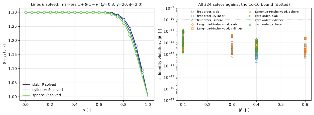
5. Breaking it on purpose: what the violation can and cannot catch
An agreement number is worth exactly what it would cost to break. One case of the sweep (the sphere at \(\phi = 2\), \(\beta = 0.3\), \(\gamma = 20\)) is solved again with one implementation error injected at a time, and three numbers are measured each time: \(\varepsilon\), the effectiveness factor \(\eta\), and the backward error.
The first four rows inject inconsistencies between the two balances: a sign, a scale, a boundary condition type, a rate evaluated at the wrong state. \(\varepsilon\) moves by more than ten orders of magnitude, and linearly in the defect: with the heat source scaled by \(1+\delta\), the combination \(\theta + (1+\delta)\beta y\) is the harmonic one, so \(\varepsilon = \delta\,(1 - y_{\min})\) exactly.
The last three rows change things that are wrong in the ordinary, expensive ways: a Newton solve stopped after one iteration, the wrong geometry index, a grid far too coarse to resolve anything. \(\varepsilon\) does not move for any of them, because \(w\) is a closed linear subsystem of the discrete equations, satisfied by every full Newton step on any grid and for any \(\nu\). They are caught by \(\eta\) and by the backward error instead. One consequence is that the severity of the sweep adds no evidential weight to \(\varepsilon\): one solve would have given the same number.
DPHI, DBETA, DGAMMA, DN = 2.0, 0.3, 20.0, 200       # the defect case, one of the sweep
D_RATE = FirstOrder(DGAMMA)
DEFECTS = [("heat source with -beta (heat_factor = -1)", {}, {"heat_factor": -1.0}),
           ("heat source 1 % too large (heat_factor = 1.01)", {}, {"heat_factor": 1.01}),
           ("film on theta only, Bi_h = 50 (y Dirichlet)", {"bi_h": 50.0}, {}),
           ("rate at theta = 1 in the energy equation", {}, {"energy_rate_isothermal": True}),
           ("sphere assembled with nu = 0", {"nu": 0}, {}),
           ("3 cells", {"n": 3}, {}),
           ("newton stopped after 1 iteration", {}, None)]


def defect_case(pellet_kw, solve_kw):
    """eps, eta, backward error and y_min of the defect case with one defect."""
    pel = TwoFieldPellet("sphere", **{"n": DN, **pellet_kw})
    if solve_kw is None:
        v, solve_kw = pel.newton_iterate(DPHI, DBETA, D_RATE, maxfev=1), {}
    else:
        v, _ = pel.solve(DPHI, DBETA, D_RATE, **solve_kw)
    return (violation(v, DBETA), pel.eta(v, DPHI),
            pel.backward_error(v, DPHI, DBETA, D_RATE, **solve_kw), float(v[:, 0].min()))


def show(x):
    """A table cell: round-off-sized values as this run's value."""
    return f"{ro(x):>16}" if abs(x) < 1e-9 else f"{x:16.4g}"


BASE = defect_case({}, {})
claims.bound("baseline_identity_violation", BASE[0], max=1e-10, basis="identity",
             note="round-off, as in the sweep")
claims.value("baseline_eta", BASE[1], rtol=1e-6)
claims.bound("baseline_backward_error", BASE[2], max=1e-12, basis="tolerance",
             note="newton tol 1e-12 with stagnation=True")
print(f"{'injected defect':<48} {'eps':>16} {'eta':>16} {'backward error':>16}")
print(f"{'none':<48} {show(BASE[0])} {show(BASE[1])} {show(BASE[2])}")
DEF = {}
for label, pkw, skw in DEFECTS:
    DEF[label] = defect_case(pkw, skw)
    e, et, be, _ = DEF[label]
    print(f"{label:<48} {show(e)} {show(et)} {show(be)}")
    brk(label, "baseline_identity_violation", e)
    brk(label, "baseline_eta", et)
    brk(label, "baseline_backward_error", be)

_e, _, _, _ymin = DEF["heat source 1 % too large (heat_factor = 1.01)"]
claims.bound("heat_scale_response", abs(_e / (0.01 * (1.0 - _ymin)) - 1.0), max=1e-9,
             basis="identity", note="eps = delta (1 - y_min) for a heat source scaled by 1 + delta")
_e2, _, _, _ymin2 = defect_case({"bi_h": 50.0}, {"heat_factor": 1.01})
brk("film on theta only, Bi_h = 50, under the 1 % heat-source probe", "heat_scale_response",
    abs(_e2 / (0.01 * (1.0 - _ymin2)) - 1.0))
BLIND = ("sphere assembled with nu = 0", "3 cells", "newton stopped after 1 iteration")
claims.bound("blind_rows_max_identity_violation", max(DEF[b][0] for b in BLIND), max=1e-10,
             basis="identity", note="the three defects eps is blind to: round-off, as in the sweep")
brk("heat source 1 % too large (the defect eps is not blind to)",
    "blind_rows_max_identity_violation", DEF["heat source 1 % too large (heat_factor = 1.01)"][0])
print(f"\nthe three defects eps is blind to (nu = 0, 3 cells, one Newton step): worst eps below "
      f"1e-10 {ro(claims['blind_rows_max_identity_violation'])}")
print(f"heat source 1 % too large: eps / (0.01 (1 - y_min)) - 1 is below 1e-9 "
      f"{ro(claims['heat_scale_response'])}")
print(f"the iterate after one Newton step has y = {TwoFieldPellet('sphere', DN).newton_iterate(DPHI, DBETA, D_RATE, 1)[0, 0]:.2f}"
      " at the centre, more reactant than at the surface, and eps is still at round-off.")

# the sweep under the same kinds of defect
_r = sweep(heat_factor=1.01)
for name, val in zip(("sweep_worst_identity_violation", "sweep_worst_backward_error",
                      "sweep_largest_eta"), sweep_metrics(_r)):
    brk("heat source 1 % too large in every sweep case", name, val)
_r = sweep_iterates(1)
for name, val in zip(("sweep_worst_identity_violation", "sweep_worst_backward_error",
                      "sweep_largest_eta"), sweep_metrics(_r)):
    brk("newton stopped after 1 iteration in every sweep case", name, val)
injected defect eps eta backward error
none (here 1.4e-13) 3.856 (here 7.2e-17)
heat source with -beta (heat_factor = -1) 0.4233 0.5181 (here 6.8e-17)
heat source 1 % too large (heat_factor = 1.01) 0.01 3.918 (here 8.8e-17)
film on theta only, Bi_h = 50 (y Dirichlet) 0.1554 5.826 (here 8.2e-17)
rate at theta = 1 in the energy equation 0.544 1.306 (here 9.5e-17)
sphere assembled with nu = 0 (here 4.1e-12) 5.009 (here 7.8e-17)
3 cells (here 1.7e-15) 5.276 (here 2.8e-17)
newton stopped after 1 iteration (here 1.4e-13) -0.01428 2.696e-05
the three defects eps is blind to (nu = 0, 3 cells, one Newton step): worst eps below 1e-10 (here 4.1e-12)
heat source 1 % too large: eps / (0.01 (1 - y_min)) - 1 is below 1e-9 (here 3.1e-12)
the iterate after one Newton step has y = 2.12 at the centre, more reactant than at the surface, and eps is still at round-off.So \(\varepsilon\) tests one thing: that the two balances see the same rate with the same sign and scale, and that the two fields carry the same kind of boundary condition. Convergence is established separately, by the backward error; the discretisation, by the comparisons in sections 6 and 7. One qualification, from the sweep rows of the break table: where the bound on \(\theta\) shortens the first Newton step, that step is no longer a Newton step for the linear subsystem, and the iterate after it does move \(\varepsilon\). That is a property of the shortened step, not a convergence check.
6. A second discretisation: what it settles and what it does not
The same problem is solved again with scipy.solve_bvp: collocation on an adaptive mesh, a different method, a different solver, and no pymrm anywhere. The domain starts at \(u_0 = 10^{-4}\) with the regular-singular series condition \(y'(u_0) = \phi^2\mathcal{R}\,u_0/(\nu+1)\), and \(\beta\) is ramped inside this solver; the pymrm solution is never used as a starting guess.
This does not make the identity check independent. solve_bvp puts the same mesh and the same collocation nodes under every component, and in its first-order system \(w\) and \(w'\) again form a closed linear pair with the rate cancelled, so the invariant is inherited for the same structural reason.
What the collocation run does contribute is the profiles. Comparing \(y(u)\) between the two solvers is a test of the pymrm discretisation that can fail. It is made on a grid ladder, against a reference whose own tolerance and start point are refined too.
PROFILE_CASES = (("slab", 1.0, 0.3, 20.0), ("cylinder", 2.0, -0.3, 20.0),
                 ("sphere", 0.5, 0.6, 20.0))            # (geometry, phi, beta, gamma)
LADDER = (100, 200, 400, 800)
U_FINE = np.linspace(1e-3, 1.0, 4001)
COLL = {c: collocation(NU[c[0]], *c[1:]) for c in PROFILE_CASES}
assert all(s.status == 0 for s in COLL.values()), "a collocation reference did not converge"


def profile_gaps(n, nu=None, at="centres"):
    """max |y_pymrm - y_collocation| per case on n cells; at="faces" reads the
    collocation solution at the cells' outer faces instead of their centres (a defect)."""
    out = []
    for c in PROFILE_CASES:
        g, phi, beta, gamma = c
        pel = TwoFieldPellet(g, n, nu=nu)
        v, _ = pel.solve(phi, beta, FirstOrder(gamma))
        x = pel.x_c if at == "centres" else pel.x_f[1:]
        out.append(float(np.max(np.abs(v[:, 0] - COLL[c].sol(x)[0]))))
    return np.array(out)


def reference_change(u0=1e-4):
    """Largest change of the collocation y(u) with its tolerance (1e-8 to 1e-9) and
    its start point (u0 to u0/100), over the cases."""
    out = 0.0
    for c in PROFILE_CASES:
        g, phi, beta, gamma = c
        base = collocation(NU[g], phi, beta, gamma, u0=u0).sol(U_FINE)[0]
        for kw in ({"tol": 1e-9, "u0": u0}, {"u0": u0 / 100}):
            alt = collocation(NU[g], phi, beta, gamma, **kw).sol(U_FINE)[0]
            out = max(out, float(np.max(np.abs(alt - base))))
    return out


def collocation_eps(heat_factor=1.0):
    out = 0.0
    for c in PROFILE_CASES:
        g, phi, beta, gamma = c
        s = COLL[c] if heat_factor == 1.0 else collocation(NU[g], phi, beta, gamma,
                                                           heat_factor=heat_factor)
        yy, tt = s.sol(U_FINE)[0], s.sol(U_FINE)[2]
        out = max(out, float(np.max(np.abs((tt - 1.0) - beta * (1.0 - yy))) / abs(beta)))
    return out


GAPS = {n: profile_gaps(n) for n in LADDER}
P_ORD = np.log2(GAPS[200] / GAPS[400])
print(f"{'case':>28} " + " ".join(f"{'n = %d' % n:>16}" for n in LADDER) + "   order 200->400")
for i, (g, phi, beta, gamma) in enumerate(PROFILE_CASES):
    lbl = f"{g} phi={phi:g} beta={beta:+.1f}"
    print(f"{lbl:>28} " + " ".join(ladder_cell(GAPS[n][i], n) for n in LADDER)
          + f"   {P_ORD[i]:.3f}")
REF_CHANGE = reference_change()
P_GUARD = float(np.min(GAPS[400] / (400**2 * EPS)))
claims.value("pymrm_vs_collocation_profile_n800", GAPS[800].max(), rtol=1e-3)
claims.bound("collocation_profile_order_min", P_ORD.min(), min=1.9, max=2.1, basis="theory",
             note="second-order finite volume, orders from 200 and 400 cells")
claims.bound("collocation_profile_order_max", P_ORD.max(), min=1.9, max=2.1, basis="theory",
             note="second-order finite volume, orders from 200 and 400 cells")
claims.bound("collocation_profile_over_roundoff", P_GUARD, min=1e3, basis="theory",
             note="gap on 400 cells over n^2 eps, the operator's condition number times eps")
claims.bound("collocation_reference_change", REF_CHANGE, max=1e-10, basis="chosen",
             note="the reference must move far less than the n = 800 gap it judges")
claims.bound("collocation_worst_identity_violation", collocation_eps(), max=1e-10,
             basis="identity", note="inherited by the collocation equations")
print(f"\nreference change with its tolerance and start point: below 1e-10 {ro(REF_CHANGE)}")
print(f"gap on 400 cells over its round-off estimate n^2 eps: at least 1e3 {ro(P_GUARD)}")
print(f"identity violation of the collocation solutions: below 1e-10 {ro(claims['collocation_worst_identity_violation'])}")
case n = 100 n = 200 n = 400 n = 800 order 200->400
slab phi=1 beta=+0.3 6.346e-05 1.594e-05 3.997e-06 1.000e-06 1.996
cylinder phi=2 beta=-0.3 1.068e-05 2.734e-06 6.918e-07 1.740e-07 1.983
sphere phi=0.5 beta=+0.6 4.687e-06 1.174e-06 2.939e-07 (here 7.4e-08) 1.998
reference change with its tolerance and start point: below 1e-10 (here 2.1e-12)
gap on 400 cells over its round-off estimate n^2 eps: at least 1e3 (here 8.3e+03)
identity violation of the collocation solutions: below 1e-10 (here 1.3e-15)display(Markdown(
f"pymrm approaches the collocation profiles at second order (orders "
f"{P_ORD.min():.2f} to {P_ORD.max():.2f}) and agrees to "
f"{claims['pymrm_vs_collocation_profile_n800']:.1e} at 800 cells. The reference "
"itself moves by less than 1e-10 when its tolerance or its start point is refined."))pymrm approaches the collocation profiles at second order (orders 1.98 to 2.00) and agrees to 1.0e-06 at 800 cells. The reference itself moves by less than 1e-10 when its tolerance or its start point is refined.
7. Cross-check against the published B1.1/B1.5 page
The Weisz-Hicks page solves a single equation, obtained by substituting the Prater relation into the species balance:
\[\nabla^2 y = \phi^2\,y\,\exp\!\left[\frac{\gamma\beta(1-y)}{1+\beta(1-y)}\right].\]
If the relation is exact, that reduced equation and this page’s two-field system must have the same solution, not merely a similar one. Three comparisons, at the \(\beta = 0.6\), \(\gamma = 20\) that B1.1 uses for its multiplicity result, and they are not of equal weight:
- \(\beta\) recovered from the two-field solution as \((\theta-1)/(1-y)\), which should be the constant \(0.6\) everywhere. This is the section 4 identity divided by \((1-y)\); its content is that this page and
B1.1attach the same value to the same symbol. A convention check. - The reduced equation solved on the same grid with the same operators. Given the discrete identity and the algebraic identity \(\gamma(1-1/\theta) \equiv \gamma\beta(1-y)/[1+\beta(1-y)]\), the two-field \(y\) is a root of the reduced discrete system, so this agreement is guaranteed. It tests that the two pages’ \(\gamma\) and \(\beta\) enter the exponent the same way: an implementation-consistency check.
- The shooting reference of
B1.1, which integrates the reduced sphere equation outward from the centre and discretises nothing. With \(s = \phi u\) the equation does not contain \(\phi\), so the radius at which \(y\) reaches 1 is \(\phi\); the centre value is root-found so that it is the \(\phi\) of the pymrm solve, on the branch through the pymrm centre value. This comparison can fail, and it tests the pymrm discretisation.
BETA_X, GAMMA_X, N_X = 0.6, 20.0, 400
PHIS_X = (0.2, 0.4, 0.8, 2.0)
B11 = load_claims("B1.1-thiele-weisz-hicks")


def cross_page(heat_factor=1.0, reduced_beta_factor=1.0):
    """Per geometry and phi: |beta recovered - 0.6|, max |y_two_field - y_reduced|, both etas."""
    out = []
    for geom in NU:
        for phi in PHIS_X:
            pel = TwoFieldPellet(geom, N_X)
            v, _ = pel.solve(phi, BETA_X, FirstOrder(GAMMA_X), heat_factor=heat_factor)
            red = ReducedPellet(geom, N_X)
            y_red = red.solve(phi, BETA_X * reduced_beta_factor, GAMMA_X, v[:, :1])
            m = (1.0 - v[:, 0]) > 1e-10
            be = float(np.max(np.abs((v[m, 1] - 1.0) / (1.0 - v[m, 0]) - BETA_X)))
            out.append((geom, phi, be, float(np.max(np.abs(v[:, 0] - y_red[:, 0]))),
                        pel.eta(v, phi)))
    return out


XP = cross_page()
print(f"{'geometry':>10} {'phi':>5} {'|beta - 0.6|':>18} {'max|y2 - yred|':>18} {'eta':>10}")
for geom, phi, be, dy, eta in XP:
    print(f"{geom:>10} {phi:5.2f} {ro(be):>18} {ro(dy):>18} {eta:10.5f}")
claims.bound("beta_recovered_vs_0p6", max(r[2] for r in XP), max=1e-8, basis="identity",
             note="round-off divided by 1 - y, which is small near the surface")
claims.bound("two_field_vs_reduced_max_dy", max(r[3] for r in XP), max=1e-10, basis="identity",
             note="the two-field y is a root of the reduced discrete system")
brk("heat source 1 % too large in the two-field solves", "beta_recovered_vs_0p6",
    max(r[2] for r in cross_page(heat_factor=1.01)))
brk("reduced equation solved with beta 1 % too large", "two_field_vs_reduced_max_dy",
    max(r[3] for r in cross_page(reduced_beta_factor=1.01)))
print(f"\nbeta recovered: 0.6 to below 1e-8; two-field against reduced: below 1e-10 in y")
print(f"B1.1 places the sphere's multiplicity window at phi from {B11['phi_fold_lower']:.4f} to "
      f"{B11['phi_fold_upper']:.4f} (its committed claims); phi = 0.4 lies inside it, so")
print("several steady states exist there; the next cell says which one the solve reaches.")
geometry phi |beta - 0.6| max|y2 - yred| eta
slab 0.20 (here 3.0e-10) (here 4.7e-12) 1.20089
slab 0.40 (here 6.4e-12) (here 5.3e-12) 26.27869
slab 0.80 (here 7.5e-12) (here 3.4e-12) 13.13936
slab 2.00 (here 7.6e-12) (here 1.2e-12) 5.25579
cylinder 0.20 (here 6.3e-11) (here 2.2e-13) 1.06167
cylinder 0.40 (here 6.2e-12) (here 9.9e-13) 1.44169
cylinder 0.80 (here 3.3e-13) (here 2.6e-13) 23.65614
cylinder 2.00 (here 5.6e-13) (here 2.8e-14) 10.10582
sphere 0.20 (here 4.8e-11) (here 3.4e-13) 1.03125
sphere 0.40 (here 1.3e-11) (here 5.1e-13) 1.15883
sphere 0.80 (here 3.0e-13) (here 2.1e-13) 31.56757
sphere 2.00 (here 3.2e-13) (here 7.5e-14) 14.55224
beta recovered: 0.6 to below 1e-8; two-field against reduced: below 1e-10 in y
B1.1 places the sphere's multiplicity window at phi from 0.2973 to 0.5719 (its committed claims); phi = 0.4 lies inside it, so
several steady states exist there; the next cell says which one the solve reaches.Which steady state. Where several steady states exist, pseudo_transient from the surface state reaches the least-ignited one, the state a start-up from surface conditions reaches. Three checks. (a) A Newton solve seeded on the hot state (\(y = 10^{-3}\), \(\theta = 1 + \beta(1-y)\)) is run for every sweep case with \(\beta > 0\); where it converges to a different state, that case has several steady states, and the page’s state is compared with it. (b) At \(\phi = 0.4\) (the sphere, \(\beta = 0.6\), \(\gamma = 20\), inside the window of B1.1) the upper state is found the same way. (c) The page’s state at \(\phi = 0.4\) is compared with a resolved \(Le = 1\) start-up, solve_ivp (BDF, error-controlled) integrating the semi-discrete system from the surface state to \(\tau = 10^3\).
N_POS = [c for c in CASES if c[3] > 0]
HOT_Y = 1e-3


def seed_state(pel, beta, y0):
    """A uniform state: reactant y0 and the temperature the identity gives with it."""
    y = np.full(pel.n, y0)
    return np.stack([y, 1.0 + beta * (1.0 - y)], axis=1)


def seeded_root(pel, phi, beta, rate, y0):
    """Newton from the uniform state seed_state(y0); None where it does not converge."""
    r = newton(lambda x: pel.residual(x, phi, beta, rate), seed_state(pel, beta, y0),
               tol=1e-12, stagnation=True, maxfev=50, bounds=pel.bounds)
    return r.x.reshape(pel.shape) if r.success else None


SOLVED = {}


def several_states(y0=HOT_Y):
    """Per beta > 0 sweep case: the largest difference between the page's state and the
    root found from the seed y0 (0 where there is none, or none with y >= 0), and
    whether the page's state is the less ignited of the two."""
    diffs, lowest = [], 0
    for kin, geom, gamma, beta, phi in N_POS:
        pel, rate = TwoFieldPellet(geom, N_SWEEP), KIN[kin](gamma)
        if (kin, geom, gamma, beta, phi) not in SOLVED:
            SOLVED[(kin, geom, gamma, beta, phi)] = pel.solve(phi, beta, rate)[0]
        v = SOLVED[(kin, geom, gamma, beta, phi)]
        w = seeded_root(pel, phi, beta, rate, y0)
        if w is None or w[:, 0].min() < -1e-6:     # no root, or an unphysical one
            diffs.append(0.0)
            continue
        diffs.append(float(np.max(np.abs(w - v))))
        lowest += bool(diffs[-1] > 1e-6 and pel.eta(v, phi) < pel.eta(w, phi))
    return np.array(diffs), lowest


_d, _low = several_states()
N_MULTI = claims.count("sweep_cases_several_states", _d, 1e-6, min_margin=0.5,
                       note="beta > 0 cases whose root from the hot seed differs from the page's")
claims.exact("sweep_several_states_page_lowest", _low,
             note="of those cases, the ones in which the page's state has the smaller eta")
print(f"{N_MULTI} of the {len(N_POS)} sweep cases with beta > 0 have a second steady state; "
      f"the page's solve is on the less ignited one in {_low} of them")
_d1, _low1 = several_states(y0=1.0)
brk("second state sought from the surface state instead of the hot state",
    "sweep_cases_several_states", int(np.sum(_d1 > 1e-6)))
brk("second state sought from the surface state instead of the hot state",
    "sweep_several_states_page_lowest", _low1)

PEL4, RATE4 = TwoFieldPellet("sphere", N_X), FirstOrder(GAMMA_X)
V4 = PEL4.solve(0.4, BETA_X, RATE4)[0]
W4 = seeded_root(PEL4, 0.4, BETA_X, RATE4, HOT_Y)


def startup(w0, le=1.0):
    """The state at tau = 1e3 of the semi-discrete start-up from w0 (solve_ivp, BDF)."""
    sol = solve_ivp(lambda t, w: _rhs(PEL4, w, 0.4, BETA_X, RATE4, le, 1.0)[0], (0.0, 1e3),
                    w0.ravel(), method="BDF", rtol=1e-8, atol=1e-11,
                    jac=lambda t, w: _rhs(PEL4, w, 0.4, BETA_X, RATE4, le, 1.0)[1])
    if not sol.success:
        raise RuntimeError(sol.message)
    return sol.y[:, -1].reshape(PEL4.shape)


S4 = startup(np.ones(PEL4.shape))
claims.value("phi04_eta_page", PEL4.eta(V4, 0.4), rtol=1e-3)
claims.value("phi04_eta_upper", PEL4.eta(W4, 0.4), rtol=1e-3)
claims.bound("phi04_state_vs_startup", float(np.max(np.abs(S4 - V4))), max=1e-8,
             basis="tolerance", note="solve_ivp BDF rtol 1e-8, atol 1e-11, at tau = 1e3")
brk("page state replaced by the root found from the hot seed", "phi04_eta_page",
    PEL4.eta(W4, 0.4))
brk("upper state sought from the surface state with the page's solve", "phi04_eta_upper",
    PEL4.eta(V4, 0.4))
brk("start-up seeded on the upper state", "phi04_state_vs_startup",
    float(np.max(np.abs(startup(W4) - V4))))
print(f"phi = 0.4, sphere, beta = 0.6, gamma = 20: the solve reaches eta = "
      f"{claims['phi04_eta_page']:.3f}, the state a start-up from the surface state reaches "
      f"(difference below 1e-8 {ro(claims['phi04_state_vs_startup'])}); the upper steady "
      f"state there has eta = {claims['phi04_eta_upper']:.1f}.")
27 of the 180 sweep cases with beta > 0 have a second steady state; the page's solve is on the less ignited one in 27 of them
phi = 0.4, sphere, beta = 0.6, gamma = 20: the solve reaches eta = 1.159, the state a start-up from the surface state reaches (difference below 1e-8 (here 4.8e-13)); the upper steady state there has eta = 44.5.PHIS_S = (0.2, 0.4, 0.8)
LADDER_S = (100, 200, 400, 800)
def shoot_errs(n, compare="phi", read="face", rtol=1e-11):
"""Relative eta error against the shooting reference per phi, sphere, n cells.
compare="centre" reads the reference at the pymrm first-cell value instead of
root-finding it at the same phi (a defect)."""
out = []
for phi in PHIS_S:
pel = TwoFieldPellet("sphere", n)
v, _ = pel.solve(phi, BETA_X, FirstOrder(GAMMA_X))
if compare == "phi":
ref = shooting_at_phi(BETA_X, GAMMA_X, phi, float(v[0, 0]), rtol=rtol)[0]
else:
ref = shooting(BETA_X, GAMMA_X, float(v[0, 0]), rtol=rtol)[1]
out.append(abs(pel.eta(v, phi, read=read) / ref - 1.0))
return np.array(out)
SH = {n: shoot_errs(n) for n in LADDER_S}
S_ORD = np.log2(SH[200] / SH[400])
print(f"{'phi':>5} " + " ".join(f"{'n = %d' % n:>16}" for n in LADDER_S) + " order 200->400")
for i, phi in enumerate(PHIS_S):
print(f"{phi:5.2f} " + " ".join(ladder_cell(SH[n][i], n) for n in LADDER_S)
+ f" {S_ORD[i]:.3f}")
S_GUARD = float(np.min(SH[400] / (400**2 * EPS)))
def shooting_tol_gap(rtol=1e-11):
"""Largest relative change of the reference eta from rtol to rtol/10."""
out = 0.0
for phi in PHIS_S:
pel = TwoFieldPellet("sphere", 800)
v, _ = pel.solve(phi, BETA_X, FirstOrder(GAMMA_X))
a = shooting_at_phi(BETA_X, GAMMA_X, phi, float(v[0, 0]), rtol=rtol)[0]
b = shooting_at_phi(BETA_X, GAMMA_X, phi, float(v[0, 0]), rtol=rtol / 10)[0]
out = max(out, abs(a / b - 1.0))
return out
claims.value("vs_shooting_reference_n800", SH[800].max(), rtol=1e-3)
claims.bound("shooting_order_min", S_ORD.min(), min=1.9, max=2.1, basis="theory",
note="second-order finite volume, orders from 200 and 400 cells")
claims.bound("shooting_order_max", S_ORD.max(), min=1.9, max=2.1, basis="theory",
note="second-order finite volume, orders from 200 and 400 cells")
claims.bound("shooting_over_roundoff", S_GUARD, min=1e3, basis="theory",
note="error on 400 cells over n^2 eps")
claims.bound("shooting_reference_tol_change", shooting_tol_gap(), max=1e-9, basis="tolerance",
note="solve_ivp rtol 1e-11 against 1e-12")
display(Markdown(
f"pymrm's $\\eta$ agrees with the shooting reference at the same $\\phi$ to "
f"{claims['vs_shooting_reference_n800']:.1e} at 800 cells, converging at orders "
f"{S_ORD.min():.3f} to {S_ORD.max():.3f}; the reference moves by less than 1e-9 "
"when its tolerance is cut tenfold. Read instead at the pymrm *first-cell* value, "
"which sits half a cell from the centre, the same comparison gives "
f"{shoot_errs(800, compare='centre').max():.1e} on the ignited state ($\\phi = 0.8$, "
"a nearly depleted centre): there $\\eta$ is so sensitive to the centre value that "
"the half-cell offset, not the error in $\\eta$, sets the number.")) phi n = 100 n = 200 n = 400 n = 800 order 200->400
0.20 3.248e-06 8.122e-07 2.031e-07 (here 5.1e-08) 2.000
0.40 1.699e-05 4.253e-06 1.064e-06 2.661e-07 1.999
0.80 1.259e-04 3.157e-05 7.900e-06 1.976e-06 1.999pymrm’s \(\eta\) agrees with the shooting reference at the same \(\phi\) to 2.0e-06 at 800 cells, converging at orders 1.999 to 2.000; the reference moves by less than 1e-9 when its tolerance is cut tenfold. Read instead at the pymrm first-cell value, which sits half a cell from the centre, the same comparison gives 4.4e-05 on the ignited state (\(\phi = 0.8\), a nearly depleted centre): there \(\eta\) is so sensitive to the centre value that the half-cell offset, not the error in \(\eta\), sets the number.
8. Where it breaks (i): a film, with unequal Biot numbers
The proof needs \(\theta + \beta y\) to be constant on the boundary. Two Dirichlet conditions give that for free. A film does not.
With \(Bi_m = k_gL/D_e\) and \(Bi_h = hL/\lambda\), the steady external balances are \(Bi_m(1-y_s)\) moles in and \(Bi_h(\theta_s-1)\) units of heat out, and these must be in the same fixed proportion as inside, so
\[\theta_s - 1 = \beta\,\frac{Bi_m}{Bi_h}\,(1-y_s).\]
The interior relation still holds exactly, referenced to the surface values: nothing inside the pellet changed. What fails is the relation people actually write, referenced to the bulk. Subtracting the two gives a closed form for the error, and it is independent of position:
\[\underbrace{(\theta - 1)}_{\text{true}} - \underbrace{\beta(1-y)}_{\text{bulk Prater}} \;=\; \beta\,(1-y_s)\left(\frac{Bi_m}{Bi_h} - 1\right).\]
So the relation survives if and only if \(Bi_m = Bi_h\), that is \(h/k_g = \lambda/D_e\). Nothing makes that happen: \(Bi_m/Bi_h = (k_g/h)\,(\lambda/D_e)\) multiplies a gas-side transfer ratio by a pellet-side transport ratio, two numbers with no reason to be reciprocal. The last column of the table is the split it produces: how much of the total temperature rise sits outside the pellet, in the film, where the internal relation has no jurisdiction.
How to read the agreement with the closed form. Both steps of the derivation (that \(\theta + \beta y\) is harmonic and that the surface balances fix its boundary value) hold for the discrete system as well, so the numerical match is forced; the same match on an 8-cell grid shows it. It confirms the algebra, not the solve. The closed form contains \(y_s\), an output of the solve, so it is a statement about the structure of the error rather than a prediction. What is contributed here is the derivation and the magnitudes.
BETA_F, GAMMA_F, PHI_F, N_F = 0.05, 20.0, 3.0, 400
FILM = [(100.0, 100.0), (100.0, 30.0), (100.0, 10.0), (100.0, 3.0), (10.0, 100.0)]


def film_case(bi_m, bi_h, n=N_F, nu=None, heat_factor=1.0, ratio="m/h"):
    """y_s, theta_s, theta_max, surface- and bulk-referenced eps, the closed form
    (``ratio="h/m"`` writes it with Bi_h/Bi_m, a defect) and the external share."""
    pel = TwoFieldPellet("sphere", n, bi_m=bi_m, bi_h=bi_h, nu=nu)
    v, _ = pel.solve(PHI_F, BETA_F, FirstOrder(GAMMA_F), heat_factor=heat_factor)
    (y_s, th_s), _ = pel.surface(v)
    r = bi_m / bi_h if ratio == "m/h" else bi_h / bi_m
    pred = abs((1.0 - y_s) * (r - 1.0))
    return dict(y_s=y_s, th_s=th_s, th_max=float(v[:, 1].max()),
                eps_s=violation(v, BETA_F, y_s, th_s), eps_b=violation(v, BETA_F), pred=pred,
                share=(th_s - 1.0) / (float(v[:, 1].max()) - 1.0))


def film_metrics(**kw):
    rows = [film_case(bm, bh, **kw) for bm, bh in FILM]
    surf = max(r["eps_s"] for r in rows)
    pred = max(abs(r["eps_b"] - r["pred"]) / r["pred"] for r in rows if r["pred"] > 1e-6)
    return rows, surf, pred


FROWS, F_SURF, F_PRED = film_metrics()
print(f"{'Bi_m':>6} {'Bi_h':>6} {'y_s':>9} {'theta_s':>9} {'theta_max':>10} "
      f"{'eps surface':>18} {'eps bulk':>11} {'closed form':>12} {'ext. dT':>8}")
for (bm, bh), r in zip(FILM, FROWS):
    eb = ro(r["eps_b"]) if r["eps_b"] < 1e-9 else f"{r['eps_b']:.4e}"
    print(f"{bm:6.0f} {bh:6.0f} {r['y_s']:9.6f} {r['th_s']:9.6f} {r['th_max']:10.6f} "
          f"{ro(r['eps_s']):>18} {eb:>11} {r['pred']:12.4e} {r['share']:8.1%}")
claims.bound("film_surface_referenced_residual", F_SURF, max=1e-10, basis="identity",
             note="the interior relation referenced to the surface values")
claims.bound("film_bulk_error_vs_closed_form", F_PRED, max=1e-9, basis="identity",
             note="relative; the discrete system satisfies both steps of the derivation")
claims.value("film_bulk_eps_bim100_bih10", FROWS[2]["eps_b"], rtol=1e-4)
claims.value("film_external_share_bih3", FROWS[3]["share"], rtol=1e-4)
claims.value("film_external_share_bih10", FROWS[2]["share"], rtol=1e-4)
_coarse = [film_case(100.0, 10.0, n=n) for n in (8, 40)]
F8 = abs(_coarse[0]["eps_b"] - _coarse[0]["pred"]) / _coarse[0]["pred"]
claims.bound("film_closed_form_match_8_cells", F8, max=1e-11, basis="identity",
             note="the match does not depend on resolution")
print(f"\nsurface-referenced Prater: exact to below 1e-10 {ro(F_SURF)}")
print(f"bulk-referenced Prater against the closed form: below 1e-9 relative {ro(F_PRED)}")
print(f"the same on 8 cells, which resolve nothing at phi = 3: below 1e-11 {ro(F8)}")
print(f"theta_max on 8 cells {_coarse[0]['th_max']:.6f}, on 40 cells {_coarse[1]['th_max']:.6f}, "
      f"on {N_F} cells {FROWS[2]['th_max']:.6f}: the solve changes, the match does not.")
Bi_m Bi_h y_s theta_s theta_max eps surface eps bulk closed form ext. dT
100 100 0.975914 1.001204 1.043748 (here 1.6e-12) (here 1.7e-12) 0.0000e+00 2.8%
100 30 0.974911 1.004181 1.047336 (here 5.8e-12) 5.8540e-02 5.8540e-02 8.8%
100 10 0.971339 1.014330 1.059165 (here 7.1e-12) 2.5795e-01 2.5795e-01 24.2%
100 3 0.109030 2.484950 2.490401 (here 9.9e-12) 2.8808e+01 2.8808e+01 99.6%
10 100 0.808118 1.000959 1.035030 (here 6.1e-12) 1.7269e-01 1.7269e-01 2.7%
surface-referenced Prater: exact to below 1e-10 (here 9.9e-12)
bulk-referenced Prater against the closed form: below 1e-9 relative (here 3.6e-11)
the same on 8 cells, which resolve nothing at phi = 3: below 1e-11 (here 1.1e-13)
theta_max on 8 cells 1.058916, on 40 cells 1.059155, on 400 cells 1.059165: the solve changes, the match does not.fig, axes = plt.subplots(1, 2, figsize=(11.5, 4.3))
show_f = [(100.0, 100.0), (100.0, 10.0), (100.0, 3.0)]
cols = plt.cm.plasma(np.linspace(0.1, 0.7, len(show_f)))
for (bi_m, bi_h), c_ in zip(show_f, cols):
pel = TwoFieldPellet("sphere", N_F, bi_m=bi_m, bi_h=bi_h)
v, _ = pel.solve(PHI_F, BETA_F, FirstOrder(GAMMA_F))
(y_s, th_s), _ = pel.surface(v)
lbl = rf"$Bi_m/Bi_h$ = {bi_m / bi_h:.0f}"
axes[0].plot(pel.x_c, v[:, 1] - 1.0, color=c_, lw=2, label=lbl)
axes[0].plot(pel.x_c, BETA_F * (1 - v[:, 0]), color=c_, lw=1.4, ls="--")
axes[1].plot(pel.x_c, (v[:, 1] - th_s) - BETA_F * (y_s - v[:, 0]), color=c_, lw=2, label=lbl)
axes[0].set_xlabel("$u$ [-]")
axes[0].set_ylabel(r"$\theta - 1$ [-]")
axes[0].set_yscale("log")
axes[0].set_title("Solid: true rise. Dashed: what bulk Prater predicts", fontsize=10)
axes[0].legend(frameon=False, fontsize=9)
axes[1].set_xlabel("$u$ [-]")
axes[1].set_ylabel(r"$(\theta-\theta_s) - \beta(y_s-y)$ [-]")
axes[1].set_ylim(-1e-11, 1e-11)
axes[1].set_title("Surface-referenced residual: zero to round-off", fontsize=10)
axes[1].legend(frameon=False, fontsize=9)
fig.tight_layout(); plt.show()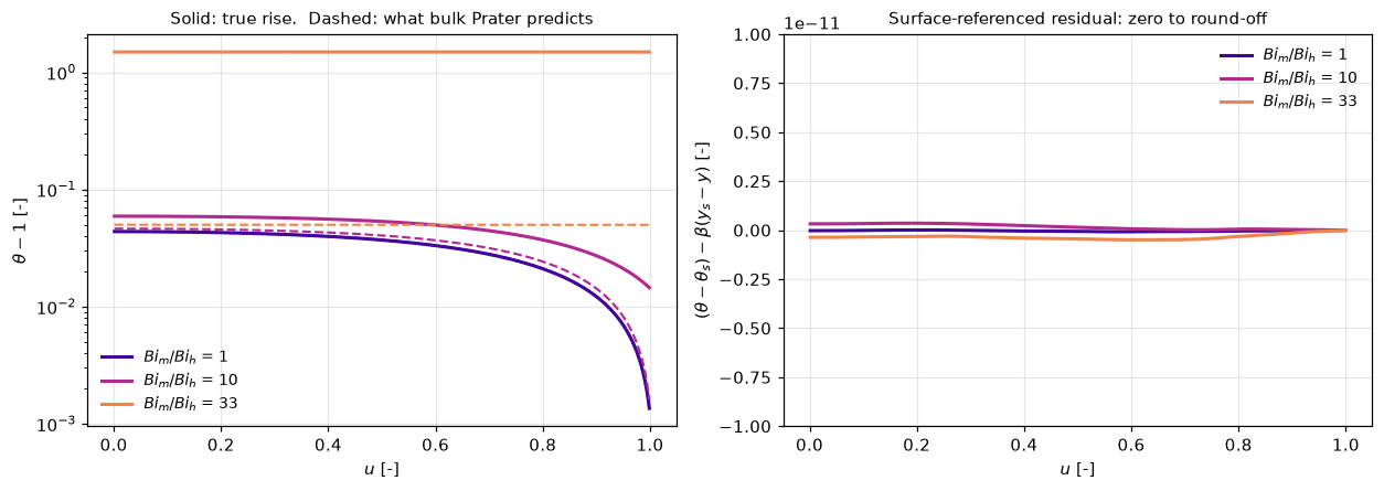
9. Where it breaks (ii): a transient, unless Le = 1
The proof also needs steady state. With accumulation, scaling time on the pellet’s mass-diffusion time \(\varepsilon_p L^2/D_e\),
\[\frac{\partial y}{\partial \tau} = \nabla^2 y - \phi^2\mathcal{R}, \qquad \frac{\partial \theta}{\partial \tau} = Le\left[\nabla^2\theta + \beta\phi^2\mathcal{R}\right], \qquad Le = \frac{\varepsilon_p\,\lambda}{\rho_p c_p D_e},\]
so that
\[\frac{\partial}{\partial\tau}(\theta + \beta y) = \nabla^2(\theta + \beta y) + (Le - 1)\left[\nabla^2\theta + \beta\phi^2\mathcal{R}\right].\]
At \(Le = 1\) the bracket disappears and \(\theta + \beta y\) obeys a homogeneous diffusion equation with constant data, so it stays at \(1+\beta\) at all times: the Prater relation is exact throughout the transient. That is a linear invariant of the semi-discrete system, which a linear multistep method with each step solved by Newton keeps to round-off, so \(Le = 1\) is a control.
Away from \(Le = 1\) the relation is violated during the transient and recovers only at steady state. The runs start a sphere at bulk conditions everywhere (so the identity holds at \(\tau = 0\)), \(\phi = 1\), \(\beta = 0.2\), \(\gamma = 20\), on 100 cells, and march with variable-step BDF2 (march in model.py: steps growing geometrically in \(\tau\), one newton solve per step with the exact Jacobian). The peak of \(\varepsilon(\tau)\) is located on a parabola in \(\log\tau\) through the largest time level and its neighbours, and taken to its limit in the step on a ladder of 50, 100 and 200 steps per decade.
BETA_T, GAMMA_T, PHI_T, N_T = 0.2, 20.0, 1.0, 100
RATE_T = FirstOrder(GAMMA_T)
WIN = {10.0: 1.0, 0.1: 5.0, 0.01: 10.0}       # Lewis number: window holding its peak
KS = (50, 100, 200)                           # steps per decade


def peak_ladder(le, n=N_T, ks=KS, order=2, heat_factor=1.0, phi=PHI_T):
    """Peak of eps(tau) per step count."""
    return [peak_of(*march(TwoFieldPellet("sphere", n), phi, BETA_T, RATE_T, le, WIN[le], k,
                           order=order, heat_factor=heat_factor)[:2])[0] for k in ks]


def richardson(p):
    """Limit in the step from the two finest rungs, second order."""
    return p[-1] + (p[-1] - p[-2]) / 3.0


def step_order(p):
    return float(np.log2(abs(p[0] - p[1]) / abs(p[1] - p[2])))


PL = {le: peak_ladder(le) for le in WIN}
TR = {le: richardson(PL[le]) for le in WIN}
T_ORD = {le: step_order(PL[le]) for le in WIN}
T_GUARD = min(abs(PL[le][-1] - PL[le][-2]) / (TR[le] * N_T**2 * EPS) for le in WIN)
IVP = {le: march_ivp(TwoFieldPellet("sphere", N_T), PHI_T, BETA_T, RATE_T, le, WIN[le])[0]
       for le in WIN}
T_IVP = max(abs(TR[le] / IVP[le] - 1.0) for le in WIN)
PL2 = {le: peak_ladder(le, n=2 * N_T, ks=(100,))[0] for le in WIN}
T_GRID = max(abs(PL2[le] / PL[le][1] - 1.0) for le in WIN)
print(f"{'Le':>6} " + " ".join(f"{'%d/decade' % k:>12}" for k in KS)
      + f" {'order':>7} {'limit':>10} {'200 cells':>11}")
for le in WIN:
    print(f"{le:6g} " + " ".join(f"{x:12.7f}" for x in PL[le])
          + f" {T_ORD[le]:7.3f} {TR[le]:10.6f} {PL2[le]:11.7f}")
claims.value("transient_worst_violation", TR[10.0], rtol=1e-3, note="Le = 10")
claims.value("transient_peak_Le0p1", TR[0.1], rtol=1e-3)
claims.value("transient_peak_Le0p01", TR[0.01], rtol=1e-3)
claims.bound("transient_step_order_min", min(T_ORD.values()), min=1.9, max=2.1, basis="theory",
             note="BDF2, orders from 50, 100 and 200 steps per decade")
claims.bound("transient_step_order_max", max(T_ORD.values()), min=1.9, max=2.1, basis="theory",
             note="BDF2, orders from 50, 100 and 200 steps per decade")
claims.bound("transient_step_over_roundoff", T_GUARD, min=1e3, basis="theory",
             note="finest step difference over n^2 eps")
claims.bound("transient_peak_vs_ivp", T_IVP, max=2e-6, basis="tolerance",
             note="BDF2 limit in the step against solve_ivp BDF at rtol 1e-9, same semi-discrete system")
claims.bound("transient_grid_change", T_GRID, max=2e-4, basis="chosen",
             note="peak on 200 cells against 100 at 100 steps per decade, relative")
print(f"\nBDF2 limit against solve_ivp (BDF, rtol 1e-9) on the same semi-discrete system: "
      f"below 2e-6 {ro(T_IVP)}")
print(f"finest step difference over its round-off estimate: at least 1e3 {ro(T_GUARD)}")
Le 50/decade 100/decade 200/decade order limit 200 cells
10 0.2520915 0.2519773 0.2519486 1.992 0.251939 0.2519601
0.1 0.1240250 0.1239840 0.1239739 2.025 0.123971 0.1239891
0.01 0.1459208 0.1459036 0.1458995 2.085 0.145898 0.1459074
BDF2 limit against solve_ivp (BDF, rtol 1e-9) on the same semi-discrete system: below 2e-6 (here 2.7e-07)
finest step difference over its round-off estimate: at least 1e3 (here 1.3e+07)LONG = {0.01: 200.0, 0.1: 200.0, 1.0: 50.0, 10.0: 50.0}
TRACE = {le: march(TwoFieldPellet("sphere", N_T), PHI_T, BETA_T, RATE_T, le, t_end, 25)
for le, t_end in LONG.items()}
claims.bound("transient_control_Le1", float(TRACE[1.0][1].max()), max=1e-11, basis="identity",
note="a linear invariant of the semi-discrete system at Le = 1")
claims.bound("transient_end_violation", max(TRACE[le][1][-1] for le in (0.1, 1.0, 10.0)),
max=1e-10, basis="chosen", note="steady state reached by the end of the window")
fig, ax = plt.subplots(figsize=(7.8, 4.6))
for le, c_ in zip(LONG, ["tab:blue", "tab:cyan", "k", "tab:red"]):
t, d, _ = TRACE[le]
ax.loglog(t[1:], np.maximum(d[1:], 1e-16), color=c_, lw=3 if le == 1.0 else 2,
label=f"Le = {le:g}")
ax.set_xlabel(r"$\tau$, time on the mass-diffusion scale [-]")
ax.set_ylabel(r"$\varepsilon$, identity violation / $\beta$ [-]")
ax.set_title(r"Prater is exact at $Le=1$ at all times, and only there")
ax.legend(frameon=False)
fig.tight_layout(); plt.show()
display(Markdown(
f"The control at $Le = 1$ stays at round-off over the whole transient (below 1e-11). "
f"Away from it the violation peaks at {claims['transient_worst_violation']:.3f} of "
f"$\\beta$ at $Le = 10$, {claims['transient_peak_Le0p1']:.3f} at $Le = 0.1$ and "
f"{claims['transient_peak_Le0p01']:.3f} at $Le = 0.01$, early in the start-up, and "
"decays as the pellet approaches its steady state: below 1e-10 by the end of the "
"window for $Le = 0.1$ and $10$, while $Le = 0.01$, the slowest, is still relaxing "
"at $\\tau = 200$. The peaks change by less than 2e-4 relative on 200 cells."))
claims.says("0.252", "transient_worst_violation")
claims.says("0.124", "transient_peak_Le0p1")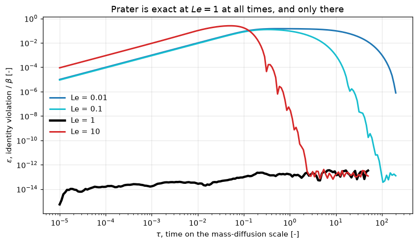
The control at \(Le = 1\) stays at round-off over the whole transient (below 1e-11). Away from it the violation peaks at 0.252 of \(\beta\) at \(Le = 10\), 0.124 at \(Le = 0.1\) and 0.146 at \(Le = 0.01\), early in the start-up, and decays as the pellet approaches its steady state: below 1e-10 by the end of the window for \(Le = 0.1\) and \(10\), while \(Le = 0.01\), the slowest, is still relaxing at \(\tau = 200\). The peaks change by less than 2e-4 relative on 200 cells.
TrueValidation
The items are not of equal weight. Several are identities of the discrete system, labelled as such; none is a comparison with a measurement. This page is tier 6, an identity proof with numerical confirmation, and it must not be described as validated against experiment.
display(Markdown(
    "| # | check | result | can it fail? |\n|---|---|---|---|\n"
    "| 1 | eq. (7) from eqs. (4)-(5); the sign of $\\beta$ in eq. (8) | "
    f"{EQ7_OK}; reading {READING} | yes: one transcribed sign flips it |\n"
    "| 2 | the identity, symbolically, any $\\mathcal{R}$, any $\\nu$ | "
    f"{IDENTITY_OK} | yes: a sign in the species balance |\n"
    f"| 3 | $\\varepsilon$ over the {len(ROWS)} sweep cases | below 1e-10 | only by an "
    "inconsistency between the balances (section 5) |\n"
    f"| 4 | backward error over the sweep | below 1e-12 | yes: it is what says they converged |\n"
    "| 5 | pymrm against collocation profiles, 800 cells | "
    f"{claims['pymrm_vs_collocation_profile_n800']:.1e}, order {P_ORD.min():.2f} to "
    f"{P_ORD.max():.2f} | yes |\n"
    "| 6 | $\\eta$ against the shooting reference at the same $\\phi$, 800 cells | "
    f"{claims['vs_shooting_reference_n800']:.1e}, order {S_ORD.min():.2f} to "
    f"{S_ORD.max():.2f} | yes |\n"
    "| 7 | $\\beta$ recovered, and the reduced equation of `B1.1` | below 1e-8, below 1e-10 | "
    "no: guaranteed by the identity; convention checks |\n"
    "| 8 | film: surface-referenced relation, closed form | below 1e-10, below 1e-9 | "
    "no: algebraic identities of the discrete system |\n"
    "| 9 | transient control at $Le = 1$; BDF2 against `solve_ivp` | below 1e-11, below 2e-6 | "
"the control no; the integrator comparison yes |\n"))| # | check | result | can it fail? |
|---|---|---|---|
| 1 | eq. (7) from eqs. (4)-(5); the sign of \(\beta\) in eq. (8) | True; reading + | yes: one transcribed sign flips it |
| 2 | the identity, symbolically, any \(\mathcal{R}\), any \(\nu\) | True | yes: a sign in the species balance |
| 3 | \(\varepsilon\) over the 324 sweep cases | below 1e-10 | only by an inconsistency between the balances (section 5) |
| 4 | backward error over the sweep | below 1e-12 | yes: it is what says they converged |
| 5 | pymrm against collocation profiles, 800 cells | 1.0e-06, order 1.98 to 2.00 | yes |
| 6 | \(\eta\) against the shooting reference at the same \(\phi\), 800 cells | 2.0e-06, order 2.00 to 2.00 | yes |
| 7 | \(\beta\) recovered, and the reduced equation of B1.1 |
below 1e-8, below 1e-10 | no: guaranteed by the identity; convention checks |
| 8 | film: surface-referenced relation, closed form | below 1e-10, below 1e-9 | no: algebraic identities of the discrete system |
| 9 | transient control at \(Le = 1\); BDF2 against solve_ivp |
below 1e-11, below 2e-6 | the control no; the integrator comparison yes |
The break table
Each row re-runs the affected computation with one thing deliberately wrong, injected through an argument of the code above, and hands the result to claims.breaks, which records whether that claim’s own check fails. The rows of section 5 are recorded above.
brk("species balance with the source's sign flipped", "identity_symbolic",
    bool(rate_cancels(species_sign=+1)[0]))
brk("eq. (5) transcribed with +H as -H", "eq7_from_eqs4_5", transcription(h_sign=-1)[0])
brk("eq. (8)'s denominator transcribed as 1 - beta(1 - y)", "eq8_beta_reading",
    transcription(eq8_denominator_sign=-1)[1])
brk("dH handed over in J/mol where kJ/mol is expected", "beta_table_max_dT_K",
    max(dt for _, dt in beta_table(dh_scale=1e3)))

# collocation and profiles
brk("pymrm pellets assembled with nu = 0", "pymrm_vs_collocation_profile_n800",
    profile_gaps(800, nu=0).max())
_pf = np.log2(profile_gaps(200, at="faces") / profile_gaps(400, at="faces"))
brk("collocation read at the cells' outer faces", "collocation_profile_order_min", _pf.min())
brk("collocation read at the cells' outer faces", "collocation_profile_order_max", _pf.max())
brk("orders fitted on 3200 and 6400 cells", "collocation_profile_over_roundoff",
    float(np.min(profile_gaps(6400) / (6400**2 * EPS))))
brk("collocation started at u0 = 1e-2 instead of 1e-4", "collocation_reference_change",
    reference_change(u0=1e-2))
brk("collocation with the heat source 1 % too large", "collocation_worst_identity_violation",
    collocation_eps(heat_factor=1.01))

# shooting
brk("reference read at the pymrm first-cell value (compare='centre')",
    "vs_shooting_reference_n800", shoot_errs(800, compare="centre").max())
_sc = np.log2(shoot_errs(200, read="cell") / shoot_errs(400, read="cell"))
brk("eta from a two-point surface gradient (read='cell')", "shooting_order_min", _sc.min())
brk("eta from a two-point surface gradient (read='cell')", "shooting_order_max", _sc.max())
brk("orders fitted on 3200 and 6400 cells", "shooting_over_roundoff",
    float(np.min(shoot_errs(6400) / (6400**2 * EPS))))
brk("shooting reference at rtol 1e-7", "shooting_reference_tol_change", shooting_tol_gap(rtol=1e-7))

# film
_fr, _fs, _ = film_metrics(heat_factor=1.01)
brk("heat source 1 % too large in the film solves", "film_surface_referenced_residual", _fs)
brk("closed form written with Bi_h/Bi_m", "film_bulk_error_vs_closed_form",
    film_metrics(ratio="h/m")[2])
_c8 = film_case(100.0, 10.0, n=8, ratio="h/m")
brk("closed form written with Bi_h/Bi_m", "film_closed_form_match_8_cells",
    abs(_c8["eps_b"] - _c8["pred"]) / _c8["pred"])
brk("sphere assembled with nu = 0", "film_bulk_eps_bim100_bih10", film_case(100.0, 10.0, nu=0)["eps_b"])
brk("Bi_m and Bi_h swapped", "film_external_share_bih3", film_case(3.0, 100.0)["share"])
brk("Bi_m and Bi_h swapped", "film_external_share_bih10", film_case(10.0, 100.0)["share"])

# transient
_ph = {le: richardson(peak_ladder(le, ks=KS, phi=0.95 * PHI_T)) for le in WIN}
brk("Thiele modulus 5 % low", "transient_worst_violation", _ph[10.0])
brk("Thiele modulus 5 % low", "transient_peak_Le0p1", _ph[0.1])
brk("Thiele modulus 5 % low", "transient_peak_Le0p01", _ph[0.01])
_be = {le: peak_ladder(le, order=1) for le in WIN}
brk("backward Euler in place of BDF2 (order=1)", "transient_step_order_min",
    min(step_order(p) for p in _be.values()))
brk("backward Euler in place of BDF2 (order=1)", "transient_step_order_max",
    max(step_order(p) for p in _be.values()))
brk("backward Euler in place of BDF2 (order=1)", "transient_peak_vs_ivp",
    max(abs(richardson(_be[le]) / IVP[le] - 1.0) for le in WIN))
_rep = {le: peak_ladder(le, ks=(KS[1], KS[1])) for le in WIN}
brk("step ladder whose last rung repeats 100 per decade", "transient_step_over_roundoff",
    min(abs(_rep[le][-1] - _rep[le][-2]) / (richardson(_rep[le]) * N_T**2 * EPS) for le in WIN))
brk("grid change read on 25 and 50 cells", "transient_grid_change",
    max(abs(peak_ladder(le, n=50, ks=(100,))[0] / peak_ladder(le, n=25, ks=(100,))[0] - 1.0)
        for le in WIN))
brk("heat source 1 % too large at Le = 1", "transient_control_Le1",
    float(march(TwoFieldPellet("sphere", N_T), PHI_T, BETA_T, RATE_T, 1.0, LONG[1.0], 25,
                heat_factor=1.01)[1].max()))
brk("heat source 1 % too large at Le = 10", "transient_end_violation",
    float(march(TwoFieldPellet("sphere", N_T), PHI_T, BETA_T, RATE_T, 10.0, LONG[10.0], 25,
heat_factor=1.01)[1][-1]))Trueprint(f"{'injected defect':<64} {'claim':<36} {'clean':>16} {'broken':>11} caught")
for name, metric, clean, broken, caught in BREAK:
kind = claims.metrics[metric]["kind"]
shown = ro(clean) if kind == "bound" else str(clean) if kind == "exact" else f"{clean:.4g}"
b = str(broken) if kind == "exact" else (ro(broken) if abs(broken) < 1e-9 else f"{broken:.4g}")
print(f"{name[:64]:<64} {metric[:36]:<36} {shown:>16} {b:>11} {'yes' if caught else 'NO'}")
_caught = {m for _, m, _, _, c in BREAK if c}
_structural = sorted(k for k, c in claims.metrics.items() if c.get("structural"))
_open = sorted(k for k in claims.metrics if k not in _caught and k not in _structural)
print(f"\n{len(BREAK)} rows; {len(_caught)} of {len(claims.metrics)} claims are failed by at "
f"least one row; structural: {', '.join(_structural) or 'none'}; "
f"open: {', '.join(_open) or 'none'}")injected defect claim clean broken caught
heat source with -beta (heat_factor = -1) baseline_identity_violation (here 1.4e-13) 0.4233 yes
heat source with -beta (heat_factor = -1) baseline_eta 3.856 0.5181 yes
heat source with -beta (heat_factor = -1) baseline_backward_error (here 7.2e-17) (here 6.8e-17) NO
heat source 1 % too large (heat_factor = 1.01) baseline_identity_violation (here 1.4e-13) 0.01 yes
heat source 1 % too large (heat_factor = 1.01) baseline_eta 3.856 3.918 yes
heat source 1 % too large (heat_factor = 1.01) baseline_backward_error (here 7.2e-17) (here 8.8e-17) NO
film on theta only, Bi_h = 50 (y Dirichlet) baseline_identity_violation (here 1.4e-13) 0.1554 yes
film on theta only, Bi_h = 50 (y Dirichlet) baseline_eta 3.856 5.826 yes
film on theta only, Bi_h = 50 (y Dirichlet) baseline_backward_error (here 7.2e-17) (here 8.2e-17) NO
rate at theta = 1 in the energy equation baseline_identity_violation (here 1.4e-13) 0.544 yes
rate at theta = 1 in the energy equation baseline_eta 3.856 1.306 yes
rate at theta = 1 in the energy equation baseline_backward_error (here 7.2e-17) (here 9.5e-17) NO
sphere assembled with nu = 0 baseline_identity_violation (here 1.4e-13) (here 4.1e-12) NO
sphere assembled with nu = 0 baseline_eta 3.856 5.009 yes
sphere assembled with nu = 0 baseline_backward_error (here 7.2e-17) (here 7.8e-17) NO
3 cells baseline_identity_violation (here 1.4e-13) (here 1.7e-15) NO
3 cells baseline_eta 3.856 5.276 yes
3 cells baseline_backward_error (here 7.2e-17) (here 2.8e-17) NO
newton stopped after 1 iteration baseline_identity_violation (here 1.4e-13) (here 1.4e-13) NO
newton stopped after 1 iteration baseline_eta 3.856 -0.01428 yes
newton stopped after 1 iteration baseline_backward_error (here 7.2e-17) 2.696e-05 yes
film on theta only, Bi_h = 50, under the 1 % heat-source probe heat_scale_response (here 3.1e-12) 16.13 yes
heat source 1 % too large (the defect eps is not blind to) blind_rows_max_identity_violation (here 4.1e-12) 0.01 yes
heat source 1 % too large in every sweep case sweep_worst_identity_violation (here 1.2e-11) 0.01 yes
heat source 1 % too large in every sweep case sweep_worst_backward_error (here 1.1e-16) (here 1.1e-16) NO
heat source 1 % too large in every sweep case sweep_largest_eta 161.6 166.9 yes
newton stopped after 1 iteration in every sweep case sweep_worst_identity_violation (here 1.2e-11) 0.1248 yes
newton stopped after 1 iteration in every sweep case sweep_worst_backward_error (here 1.1e-16) 0.02548 yes
newton stopped after 1 iteration in every sweep case sweep_largest_eta 161.6 5.448 yes
heat source 1 % too large in the two-field solves beta_recovered_vs_0p6 (here 3.0e-10) 0.006 yes
reduced equation solved with beta 1 % too large two_field_vs_reduced_max_dy (here 5.3e-12) 0.0144 yes
second state sought from the surface state instead of the hot st sweep_cases_several_states 27 0 yes
second state sought from the surface state instead of the hot st sweep_several_states_page_lowest 27 0 yes
page state replaced by the root found from the hot seed phi04_eta_page 1.159 44.55 yes
upper state sought from the surface state with the page's solve phi04_eta_upper 44.55 1.159 yes
start-up seeded on the upper state phi04_state_vs_startup (here 4.8e-13) 0.969 yes
species balance with the source's sign flipped identity_symbolic True False yes
eq. (5) transcribed with +H as -H eq7_from_eqs4_5 True False yes
eq. (8)'s denominator transcribed as 1 - beta(1 - y) eq8_beta_reading + none yes
dH handed over in J/mol where kJ/mol is expected beta_table_max_dT_K 320 3.2e+05 yes
pymrm pellets assembled with nu = 0 pymrm_vs_collocation_profile_n800 1e-06 0.9583 yes
collocation read at the cells' outer faces collocation_profile_order_min (here 2.0e+00) 0.9965 yes
collocation read at the cells' outer faces collocation_profile_order_max (here 2.0e+00) 0.9998 yes
orders fitted on 3200 and 6400 cells collocation_profile_over_roundoff (here 8.3e+03) 0.1201 yes
collocation started at u0 = 1e-2 instead of 1e-4 collocation_reference_change (here 2.1e-12) 1.443e-07 yes
collocation with the heat source 1 % too large collocation_worst_identity_violation (here 1.3e-15) 0.009996 yes
reference read at the pymrm first-cell value (compare='centre') vs_shooting_reference_n800 1.976e-06 4.424e-05 yes
eta from a two-point surface gradient (read='cell') shooting_order_min (here 2.0e+00) 0.9987 yes
eta from a two-point surface gradient (read='cell') shooting_order_max (here 2.0e+00) 1.007 yes
orders fitted on 3200 and 6400 cells shooting_over_roundoff (here 5.7e+03) 0.2321 yes
shooting reference at rtol 1e-7 shooting_reference_tol_change (here 8.7e-12) 6.497e-08 yes
heat source 1 % too large in the film solves film_surface_referenced_residual (here 9.9e-12) 0.008983 yes
closed form written with Bi_h/Bi_m film_bulk_error_vs_closed_form (here 3.6e-11) 32.33 yes
closed form written with Bi_h/Bi_m film_closed_form_match_8_cells (here 1.1e-13) 9 yes
sphere assembled with nu = 0 film_bulk_eps_bim100_bih10 0.2579 0.3724 yes
Bi_m and Bi_h swapped film_external_share_bih3 0.9963 0.02738 yes
Bi_m and Bi_h swapped film_external_share_bih10 0.2422 0.02739 yes
Thiele modulus 5 % low transient_worst_violation 0.2519 0.1966 yes
Thiele modulus 5 % low transient_peak_Le0p1 0.124 0.1121 yes
Thiele modulus 5 % low transient_peak_Le0p01 0.1459 0.1329 yes
backward Euler in place of BDF2 (order=1) transient_step_order_min (here 2.0e+00) 0.9739 yes
backward Euler in place of BDF2 (order=1) transient_step_order_max (here 2.1e+00) 0.9962 yes
backward Euler in place of BDF2 (order=1) transient_peak_vs_ivp (here 2.7e-07) 0.002424 yes
step ladder whose last rung repeats 100 per decade transient_step_over_roundoff (here 1.3e+07) (here 0.0e+00) yes
grid change read on 25 and 50 cells transient_grid_change (here 6.8e-05) 0.001078 yes
heat source 1 % too large at Le = 1 transient_control_Le1 (here 3.6e-13) 0.002842 yes
heat source 1 % too large at Le = 10 transient_end_violation (here 3.3e-13) 0.002842 yes
67 rows; 46 of 46 claims are failed by at least one row; structural: none; open: noneThe rows that do not fail their claim are the point of section 5: the identity violation is blind to a Newton solve stopped after one iteration, to the wrong geometry index and to a 3-cell grid, and the backward error is blind to every defect that still leaves a converged solve of a wrong model. Each of those defects is caught by another claim in the same row group.
What this page cannot conclude. The assumption that both balances share one reaction rate is not tested, nor are a variable \(D_e\) and \(\lambda\), where only the Kirchhoff-transformed relation between the potentials survives. Zero-order kinetics is swept at small \(\phi\) only, because above a threshold a dead core forms and no steady state exists to test. Nothing here validates the physics against a measurement.
What pymrm adds
Nothing to the identity itself. Prater’s result is exact and its proof is two lines. Reproducing it numerically confirms an implementation, not a theorem.
What the computation adds is the size of the error when the assumptions fail, which the 1958 result could only assume away:
- A film with \(Bi_m \neq Bi_h\). The interior relation survives, referenced to the surface. The bulk-referenced form, the one that gets written down, is wrong by \(\beta(1-y_s)(Bi_m/Bi_h-1)\), uniformly in position. That closed form is derived here, not in either source; the numerics agree with it to round-off because the derivation holds step for step in the discrete system, so what the computation supplies is the magnitude: how much of the temperature rise moves out of the pellet and into the film.
- A transient with \(Le \neq 1\). The relation is a linear invariant of the time-dependent system exactly when \(Le = 1\); the computation keeps it to round-off there and measures the violation elsewhere (section 9), peaking early in the start-up and decaying at steady state. A quasi-steady pellet model that carries the Prater relation into a dynamic simulation makes an error of this size.
- Geometry, kinetics and boundary type as arguments.
nu = 0, 1, 2, a swapped rate function and a film on either field cover the whole sweep and the defect table with one class. The two-field state is oneBlockLayout.from_fieldslayout, the coupling block is oneconstruct_coefficient_matrixcall,pseudo_transientreaches every case of the sweep from the surface state without a path in \(\beta\), and the same operators march the transient with onenewtonsolve per step.
And the identity is a cheap unit test for any non-isothermal pellet code, for one specific class of bug. Solve both balances, evaluate \((\theta-1)-\beta(1-y)\), and a number that is not at round-off means the two balances disagree about the reaction: a wrong sign or scale on the heat source, a rate evaluated at inconsistent states, or two fields carrying different kinds of boundary condition. The response is exact: a heat source scaled by \(1+\delta\) gives \(\varepsilon = \delta(1-y_{\min})\).
It will not tell you anything else. \(\varepsilon\) stays at round-off for a Newton iterate that has not converged (even one with more reactant at the centre than at the surface), for the wrong geometry index, and for a grid three cells wide. Those need the backward error, a comparison against an independent method, and grid refinement, all of which are on this page because \(\varepsilon\) cannot stand in for them.
Reuse
| Change | Where |
|---|---|
| Different geometry | TwoFieldPellet(geom=...), or a callable nu in construct_div |
| Different kinetics | pass any rate(y, theta) returning the rate and its two partial derivatives |
| External film | TwoFieldPellet(..., bi_m=, bi_h=); both Robin rows have \(a = 1\) |
| Transient | march(pellet, phi, beta, rate, le, t_end, per_decade); the operators are the steady ones |
| More species | widen the field axis, BlockLayout.from_fields([...], (n,)), temperature last |
| Reversible or multiple reactions | the identity needs one shared rate; with several, one relation per independent reaction extent |
The trap this page exists to flag. The Prater relation is usually quoted with the bulk concentration and bulk temperature, because that is what is measurable. That version is only correct when the surface and bulk coincide, or when \(Bi_m = Bi_h\). Referenced to the surface it is exact; referenced to the bulk it is not, and section 8 gives the error in closed form.
Comparing \(\eta\) with a shooting reference. Compare at the same \(\phi\). The first cell’s value of a finite-volume solution is not the centre value; on an ignited state, where the centre is nearly depleted, \(\eta\) is so sensitive to the centre value that reading the reference there measures the half-cell offset instead of the error in \(\eta\) (section 7).
Reading Weisz and Hicks. The scan’s text layer is unusable for equations: eq. (7) comes out as AT = T - To = - F and eq. (2) as [grad ~1,~~. Render journal page 266 at 600 dpi and read it. The prose OCRs acceptably; the numbers and symbols do not. The same trap is recorded for B3.1 and in docs/pdf-findings.md.
Related pages. B1.1/B1.5, the non-isothermal pellet this relation makes solvable, where \(\beta\) is a curve label; B1.2 Aris generalised modulus; B1.4 Weisz-Prater criterion (the observable-quantity counterpart of \(\beta\)); D1.4 fixed bed with resolved pellets, where the film conditions of section 8 are supplied by the reactor; J4.7 immobilised enzyme particle, the same S3 structure.
References
Prater, C. D. (1958). The temperature produced by heat of reaction in the interior of porous particles. Chemical Engineering Science 8(3-4), 284-286. doi:10.1016/0009-2509(58)85035-6. The origin of the result; not consulted for this page, because no copy is available. Cited as Weisz and Hicks cite it (“[11] PRATER C. D., Chem. Engng. Sci. 1958 8 284”), with the DOI resolved and checked against that volume and page.
Weisz, P. B. and Hicks, J. S. (1962). The behaviour of porous catalyst particles in view of internal mass and heat diffusion effects. Chemical Engineering Science 17(4), 265-275. doi:10.1016/0009-2509(62)85005-2. The source actually read. Eqs. (4), (5), (7) and (8) above are transcribed from a 600 dpi render of journal page 266.
Damköhler, G. (1943). Z. Phys. Chem. A193, 16, cited by Weisz and Hicks as having obtained the relation for the spherical particle.
# Claims: prints every registered number, writes agreement.json for CI, and
# raises when a claim fails its own check or has no break row.
claims.report();   # the semicolon keeps the notebook from echoing the payload
Claims for B1.6:
identity_symbolic = True exact exact
eq7_from_eqs4_5 = True exact exact
eq8_beta_reading = '+' exact exact
beta_table_max_dT_K = 320 value rtol 1e-09
sweep_worst_identity_violation = (here 1.2e-11) bound bound <= 1e-10 [identity]
sweep_worst_backward_error = (here 1.1e-16) bound bound <= 1e-12 [tolerance]
sweep_largest_eta = 161.65 value rtol 0.001
baseline_identity_violation = (here 1.4e-13) bound bound <= 1e-10 [identity]
baseline_eta = 3.856 value rtol 1e-06
baseline_backward_error = (here 7.2e-17) bound bound <= 1e-12 [tolerance]
heat_scale_response = (here 3.1e-12) bound bound <= 1e-09 [identity]
blind_rows_max_identity_violation = (here 4.1e-12) bound bound <= 1e-10 [identity]
pymrm_vs_collocation_profile_n800 = 1.0004e-06 value rtol 0.001
collocation_profile_order_min = (here 2.0e+00) bound bound [1.9, 2.1] [theory]
collocation_profile_order_max = (here 2.0e+00) bound bound [1.9, 2.1] [theory]
collocation_profile_over_roundoff = (here 8.3e+03) bound bound >= 1000 [theory]
collocation_reference_change = (here 2.1e-12) bound bound <= 1e-10 [chosen]
collocation_worst_identity_violation = (here 1.3e-15) bound bound <= 1e-10 [identity]
beta_recovered_vs_0p6 = (here 3.0e-10) bound bound <= 1e-08 [identity]
two_field_vs_reduced_max_dy = (here 5.3e-12) bound bound <= 1e-10 [identity]
sweep_cases_several_states = 27 exact exact, margin 1
sweep_several_states_page_lowest = 27 exact exact
phi04_eta_page = 1.1588 value rtol 0.001
phi04_eta_upper = 44.548 value rtol 0.001
phi04_state_vs_startup = (here 4.8e-13) bound bound <= 1e-08 [tolerance]
vs_shooting_reference_n800 = 1.9756e-06 value rtol 0.001
shooting_order_min = (here 2.0e+00) bound bound [1.9, 2.1] [theory]
shooting_order_max = (here 2.0e+00) bound bound [1.9, 2.1] [theory]
shooting_over_roundoff = (here 5.7e+03) bound bound >= 1000 [theory]
shooting_reference_tol_change = (here 8.7e-12) bound bound <= 1e-09 [tolerance]
film_surface_referenced_residual = (here 9.9e-12) bound bound <= 1e-10 [identity]
film_bulk_error_vs_closed_form = (here 3.6e-11) bound bound <= 1e-09 [identity]
film_bulk_eps_bim100_bih10 = 0.25795 value rtol 0.0001
film_external_share_bih3 = 0.99634 value rtol 0.0001
film_external_share_bih10 = 0.24221 value rtol 0.0001
film_closed_form_match_8_cells = (here 1.1e-13) bound bound <= 1e-11 [identity]
transient_worst_violation = 0.25194 value rtol 0.001
transient_peak_Le0p1 = 0.12397 value rtol 0.001
transient_peak_Le0p01 = 0.1459 value rtol 0.001
transient_step_order_min = (here 2.0e+00) bound bound [1.9, 2.1] [theory]
transient_step_order_max = (here 2.1e+00) bound bound [1.9, 2.1] [theory]
transient_step_over_roundoff = (here 1.3e+07) bound bound >= 1000 [theory]
transient_peak_vs_ivp = (here 2.7e-07) bound bound <= 2e-06 [tolerance]
transient_grid_change = (here 6.8e-05) bound bound <= 0.0002 [chosen]
transient_control_Le1 = (here 3.6e-13) bound bound <= 1e-11 [identity]
transient_end_violation = (here 3.3e-13) bound bound <= 1e-10 [chosen]