# Colab environment cell - no-op if pymrm is already installed
try:
    import pymrm
except ImportError:
%pip install -q pymrm pyyamlChapman–Enskog binary diffusion
sec:A
struct:S3
tier:T0
data:tier2
phase:gas
A diffusivity derived from the intermolecular potential rather than fitted to diffusion data — put against the 50 measured pairs Chapman & Cowling print, and asked how much of its accuracy is the theory and how much is the two-parameter fit underneath it.
Chapman–Enskog binary diffusion
Catalog ID: A4.6 · Structure: S3 (scalar diffusion) · Tier: T0
Almost every diffusivity a chemical engineer uses is a correlation: a functional form with constants regressed against the quantity it predicts. The Chapman–Enskog result is not. It is the first Sonine-polynomial solution of the Boltzmann equation, and it delivers \(D_{12}\) from the intermolecular potential and the molecular masses with nothing fitted to a diffusion measurement.
That makes one question worth asking, and this page asks it: how well does a first-principles transport coefficient predict measurement?
Chapman & Cowling supply everything needed to answer it in printed tables — the collision integrals (Table 6), the force constants (Table 17), the pure-gas viscosities and molecular weights (Table 11), and 50 measured \(D_{12}\) values at S.T.P. with their literature references (Table 22). No figure is digitised anywhere on this page.
The answer has two halves, and the second is the important one. The prediction lands within a few per cent of measurement. But the Lennard-Jones constants it needs are themselves a two-parameter fit to viscosity, and the book prints a second, equally published set of constants for the same molecules obtained from virial coefficients. Swapping one set for the other more than doubles the disagreement. So the headline number is a joint statement about kinetic theory and about where its parameters came from, and this page separates the two rather than reporting the flattering half.
Background
What the theory is. Chapman and Enskog independently solved the Boltzmann equation for a slightly non-uniform gas by expanding the velocity distribution about the local Maxwellian and projecting onto Sonine polynomials. The transport coefficients come out as ratios of collision integrals \(\Omega^{(l)}_{12}(r)\) — averages of the deflection produced by a binary encounter, weighted over impact parameter and relative speed. Nothing in the derivation is empirical; the only input is the intermolecular potential.
Why this is not another correlation. The distinction matters because it changes what a comparison against data means. A correlation fitted to \(D_{12}\) data and then tested against \(D_{12}\) data is measuring the quality of a fit. Chapman–Enskog with force constants taken from viscosity is a genuine out-of-sample prediction: the fitted quantity (viscosity of a pure gas) and the predicted quantity (diffusion in a binary mixture) are different properties of different systems, connected only by the assumed potential.
That is the sense in which the comparison below is out of sample, and it is worth being precise about its limits, because a two-parameter fit is still a two-parameter fit:
- the constants \(\varepsilon/k\) and \(\sigma\) of Table 17 are obtained, the book says on p. 235, “mainly by Hirschfelder, Bird and Spotz … from the viscosities of various gases”, by sliding a standard \(\log(\mu/\sqrt{T})\)–\(\log T\) curve onto the measured one;
- the unlike-pair constants are then assumed through combination rules, \(\varepsilon_{12} = \sqrt{\varepsilon_1 \varepsilon_2}\) and \(\sigma_{12} = \tfrac12(\sigma_1 + \sigma_2)\) — the book states both, the first on p. 262 and the second at eq. (14.2, 1);
- the collision integrals of Table 6 are numerical integrations of the 12,6 potential, fitted to nothing at all.
So no diffusion measurement enters the prediction. But viscosity is itself a transport property governed by collision integrals of the same potential, so the viscosity fit is “close” to diffusion in a way that, say, a fit to second virial coefficients is not. Section Results measures exactly how much that proximity is worth.
The book’s own caveats, which this page carries. Section 14.2 opens: “Observations of the mutual diffusion of pairs of gases are difficult to make, and such observations as have been made are liable to a fairly large experimental error. This should be borne in mind when comparing theory with experiment.” Section 14.32 closes: “The accuracy of \(D_{12}\) measurements is not high, and the values quoted may, in unfavourable cases, be in error by several per cent.” Section 14.4 says only that predictions from combination-rule constants “in general agree fairly well with the experimental values”. Putting a number on “fairly well” is what this page adds.
The published model
Source. Chapman, S. and Cowling, T. G. (1970), The Mathematical Theory of Non-Uniform Gases, 3rd edn, Cambridge University Press. This is the origin, not a reprint: the book is the primary account of the solution the case is named for, by one of the two people it is named after. There is therefore no reference_read_from.
The PDF on disk is a complete 448-page scan (CCITT-G4 bilevel, 300 ppi native) with an ABBYY FineReader text layer. The prose layer is good; the numbers are not — the 1970 typesetting uses a raised mid-dot decimal separator that the OCR drops, and leading zeros come back as the letter “o” (Table 6’s 0·4291 reads as o-4291). Every numeral on this page was read off a 300 dpi render, cropped, at native resolution. Rendering at 600 dpi would be pure interpolation of a 1-bit image.
The first approximation (eq. 14.2, 4), for the Lennard-Jones 12,6 and the exp;6 models:
\[ [D_{12}]_1 \;=\; \frac{3}{8\,n\,\sigma_{12}^2\,\mathscr{W}^{(1)}_{12}(1)} \left(\frac{kT(m_1+m_2)}{2\pi m_1 m_2}\right)^{1/2}, \]
where \(\mathscr{W}^{(1)}_{12}(1)\) is a function of \(kT/\varepsilon_{12}\) alone, tabulated in Table 6. Setting \(\mathscr{W}^{(1)}_{12}(1) = 1\) and \(\sigma_{12} = \tfrac12(\sigma_1+\sigma_2)\) recovers eq. (14.2, 1), the rigid-elastic-sphere result — which is used below as the null model, because it is the same expression with the collision integral deleted.
The 12,6 potential itself is eq. (10.42, 1), \(V(r) = 4\varepsilon_{12}\{(\sigma_{12}/r)^{12} - (\sigma_{12}/r)^6\}\), and \(r_m \equiv 2^{1/6}\sigma\) is the separation of minimum energy (p. 236).
The second approximation (eqs. 14.21, 1–6). Unlike the first, it depends on composition:
\[ [D_{12}]_2 = \frac{[D_{12}]_1}{1-\Delta},\qquad \Delta = 5\mathrm{C}^2\, \frac{M_1^2\mathrm{P}_1 x_1^2 + M_2^2\mathrm{P}_2 x_2^2 + \mathrm{P}_{12}x_1x_2} {\mathrm{Q}_1 x_1^2 + \mathrm{Q}_2 x_2^2 + \mathrm{Q}_{12}x_1x_2}, \]
\[ \mathrm{P}_1 = M_1 \mathrm{E}/[\mu_1]_1, \quad \mathrm{P}_{12} = 3(M_1-M_2)^2 + 4M_1M_2\mathrm{A}, \] \[ \mathrm{Q}_1 = \mathrm{P}_1\left(6M_2^2 + 5M_1^2 - 4M_1^2\mathrm{B} + 8M_1M_2\mathrm{A}\right), \] \[ \mathrm{Q}_{12} = 3(M_1-M_2)^2(5-4\mathrm{B}) + 4M_1M_2\mathrm{A}(11-4\mathrm{B}) + 2\mathrm{P}_1\mathrm{P}_2, \]
with \(M_i = m_i/(m_1+m_2)\), \(\mathrm{Q}_2\) the \(1\leftrightarrow 2\) image of \(\mathrm{Q}_1\) (“with a similar relation for \(\mathrm{Q}_2\)”), and \(\mathrm{E} = kT/(8M_1M_2\Omega^{(1)}_{12}(1))\) from eq. (9.8, 8). A, B, C are the pure-number ratios of collision integrals defined at eq. (9.8, 7) and tabulated alongside \(\mathscr{W}\) in Table 6.
One reading that had to be reconstructed, and how. Table 6’s third column is headed by a fraction whose glyph is destroyed in the scan — it is a solid blob at 300 ppi, and it cannot be read visually at any magnification. It is \(\tfrac12\mathscr{W}^{(2)}_{12}(2)\), not \(\tfrac13\), and this is established twice from printed material rather than guessed: eq. (9.8, 7) defines \(\mathrm{A} \equiv \Omega^{(2)}_{12}(2)/5\Omega^{(1)}_{12}(1)\), and eq. (10.2, 1) fixes the rigid-sphere normalisation \(\mathscr{W}^{(1)}(1) = 1\), \(\mathscr{W}^{(2)}(2) = 2\); and, independently, the collision integrals are recomputed from the 12,6 potential by quadrature in Validation. Both tests are quantitative and both are reported below. The prior source note on this book recorded the fraction as \(\tfrac13\); it is not.
This has no effect on any diffusivity — only \(\mathscr{W}^{(1)}_{12}(1)\) enters \([D_{12}]_1\), and A is printed as its own column. It is recorded because the next reader of this table will meet the same blob.
import math, sys, urllib.request
from pathlib import Path

# Make shared/gallery_utils.py importable locally and on Colab
if not any("shared" in p for p in sys.path):
    local = Path.cwd()
    for _ in range(4):
        if (local / "shared" / "gallery_utils.py").is_file():
            sys.path.insert(0, str(local / "shared")); break
        local = local.parent
    else:
        url = ("https://raw.githubusercontent.com/computational-chemical-engineering/pymrm-gallery/"
               "main/shared/gallery_utils.py")
        urllib.request.urlretrieve(url, "gallery_utils.py")
        sys.path.insert(0, ".")

import numpy as np
import pandas as pd
import matplotlib.pyplot as plt
import scipy.sparse as sp
from IPython.display import Markdown, display
from scipy.constants import N_A, atm
from scipy.constants import k as kB_SI
from scipy.interpolate import CubicSpline
from scipy.optimize import brentq

from gallery_utils import cite_data, load_data, load_meta, report_agreement
from pymrm import (construct_coefficient_matrix, construct_div, construct_grad,
                   interp_cntr_to_stagg, newton)

np.random.seed(0)          # nothing here is stochastic; seeded anyway
plt.rcParams.update({"figure.dpi": 110, "axes.grid": True, "grid.alpha": 0.3})
PAGE = "A4.6-chapman-enskog"
T_STP = 273.15             # K - section 14.32: "reduced to 0 degC"
kB = kB_SI * 1e7           # erg/K   (the book works in c.g.s. throughout)
n_STP = atm * 10 / (kB * T_STP)     # molecules/cm^3 at 1 atm, 0 degC

t6 = load_data("chapman-cowling-1970-table6.csv", page=PAGE)
t11 = load_data("chapman-cowling-1970-table11.csv", page=PAGE)
t17 = load_data("chapman-cowling-1970-table17.csv", page=PAGE)
t22 = load_data("chapman-cowling-1970-table22.csv", page=PAGE)
print(cite_data(load_meta("chapman-cowling-1970-table22.csv", page=PAGE)))
print(f"Table 6 rows {len(t6)} | Table 11 gases {len(t11)} | "
      f"Table 17 gases {len(t17)} | Table 22 pairs {len(t22)}")
print(f"Loschmidt number at 1 atm, {T_STP} K : n = {n_STP:.5e} /cm^3")
Chapman, Sydney; Cowling, T. G. (1970) — The Mathematical Theory of Non-Uniform Gases: An Account of the Kinetic Theory of Viscosity, Thermal Conduction and Diffusion in Gases, 3rd edition, prepared in co-operation with D. Burnett. Cambridge University Press. Reissued in the Cambridge Mathematical Library with a Foreword by Carlo Cercignani, 1990; reprinted 1993. ISBN 0 521 40844 X. Table 22, book p. 263.
— table
Table 6 rows 16 | Table 11 gases 24 | Table 17 gases 18 | Table 22 pairs 50
Loschmidt number at 1 atm, 273.15 K : n = 2.68678e+19 /cm^3Parameters and assumptions
State. Table 22 is headed “Coefficients of diffusion at S.T.P.” and section 14.32 says the values are “reduced to 0 °C”, with a footnote fixing the units: “Here (and throughout this book) values of \(D_{12}\) are expressed in cm²/sec.” So \(T = 273.15\) K. The pressure is not stated in words — but it does not have to be assumed, because the book prints a column that pins it: the \(\sigma_{12}\) column of Table 22 is, by section 14.32, the value obtained from each measured \(D_{12}\) through eq. (14.2, 1). Inverting that equation and asking which pressure reproduces the printed column settles the convention from the book’s own arithmetic. The next cell does it.
Molar masses come from Table 11, not from a modern periodic table — the book prints them (H2 2.016, A 39.944, Xe 131.30), so nothing external is needed. Pure-gas viscosities for the second approximation come from the same table.
Physical constants are modern CODATA values via scipy.constants. The 1970 values of \(k\) and \(N_A\) differ in the fifth significant figure, which is far below every number reported here; the choice is stated rather than hidden.
Which pairs can be used. Table 22 has 50 measured pairs. Table 17 gives 12,6 force constants for 18 gases, and three species appearing in Table 22 — NH₃, C₂H₄, C₂H₆ — are not among them. Those 11 pairs are dropped, leaving 39. No pair is dropped for any other reason: there is no selection on how well it agrees.
Two polar species are kept, deliberately. SO₂ and HCl have permanent dipole moments, and p. 235 says of the 12,6 model that “for polar gases the attractive part of the molecular potential energy includes a term proportional to \(r^{-3}\) … and the fit with experiment is less close”. Only H₂–SO₂ survives the Table 17 filter. It is kept and flagged rather than removed, because removing it would be a selection on the model’s known weakness.
# ---- which pressure convention does the book's own sigma12 column imply? -----
M = dict(zip(t11.formula, t11.M))
mu_pure = dict(zip(t11.formula, t11.mu_1e7_poise * 1e-7))         # poise
sig_visc11 = dict(zip(t11.formula, t11.sigma_1e8_cm))             # 1e-8 cm, Table 11
eps_lj = dict(zip(t17.formula, t17.eps_k_visc))                   # K,      Table 17
sig_lj = dict(zip(t17.formula, t17.sigma_visc_1e8_cm))            # 1e-8 cm, Table 17
eps_other = dict(zip(t17.formula, pd.to_numeric(t17.eps_k_other, errors="coerce")))
sig_other = dict(zip(t17.formula, pd.to_numeric(t17.sigma_other_1e8_cm, errors="coerce")))

m1_all = np.array([M[g] / N_A for g in t22.gas1])
m2_all = np.array([M[g] / N_A for g in t22.gas2])


def sigma12_from_D(D12, m1, m2, T, n):
    """Invert eq. (14.2, 1): the rigid-sphere sigma_12 that a measured D12 implies."""
    return np.sqrt(3 / (8 * n * D12) * np.sqrt(kB * T * (m1 + m2) / (2 * np.pi * m1 * m2))) * 1e8


rows = []
for label, T, p_dyn in [("1 atm, 273.15 K", 273.15, atm * 10), ("1 bar, 273.15 K", 273.15, 1e6),
                        ("1 atm, 273.16 K", 273.16, atm * 10), ("1 atm, 293.15 K", 293.15, atm * 10)]:
    s = sigma12_from_D(t22.D12_cm2_s.values, m1_all, m2_all, T, p_dyn / (kB * T))
    d = s - t22.sigma12_1e8_cm.values
    rows.append((label, np.abs(d).max(), d.mean()))
print(f"{'convention':<18}{'max |dev|':>11}{'mean signed':>13}   (printed to 3 s.f., i.e. +-0.005)")
for label, mx, mn in rows:
    print(f"{label:<18}{mx:>11.5f}{mn:>+13.5f}")
sig_roundtrip_max = rows[0][1]
sig_roundtrip_bias = rows[0][2]
sig_roundtrip_bar_bias = rows[1][2]
convention max |dev| mean signed (printed to 3 s.f., i.e. +-0.005)
1 atm, 273.15 K 0.00509 +0.00016
1 bar, 273.15 K 0.03214 +0.02257
1 atm, 273.16 K 0.00520 +0.00026
1 atm, 293.15 K 0.24129 +0.18485display(Markdown(
f"Only the 1 atm reading is unbiased: the mean signed residual is "
f"**{sig_roundtrip_bias:+.5f}** against a printed resolution of ±0.005, while 1 bar leaves a "
f"systematic **{sig_roundtrip_bar_bias:+.5f}** — {abs(sig_roundtrip_bar_bias/sig_roundtrip_bias):.0f}× larger and one-signed. "
f"The worst single residual at 1 atm is {sig_roundtrip_max:.5f}, inside one rounding unit for all "
f"{len(t22)} pairs. **S.T.P. here is 1 atm and 0 °C**, established from the book rather than assumed."))Only the 1 atm reading is unbiased: the mean signed residual is +0.00016 against a printed resolution of ±0.005, while 1 bar leaves a systematic +0.02257 — 137× larger and one-signed. The worst single residual at 1 atm is 0.00509, inside one rounding unit for all 50 pairs. S.T.P. here is 1 atm and 0 °C, established from the book rather than assumed.
The data
Four printed tables, all transcribed by eye from cropped 300 dpi renders on 2026-08-05, with a provenance sidecar each.
| file | what it is | tier |
|---|---|---|
chapman-cowling-1970-table6.csv |
16 rows of collision integrals for the 12,6 model | 6 (computed) |
chapman-cowling-1970-table11.csv |
24 gases: molecular weight, viscosity at S.T.P., viscosity diameter | 2 (measured μ) |
chapman-cowling-1970-table17.csv |
18 gases: 12,6 force constants, from viscosity and from other data | 6 (fitted) |
chapman-cowling-1970-table22.csv |
50 measured \(D_{12}\) at S.T.P., with the book’s own literature references | 2 (measured) |
No dataset is borrowed from another page. The cross-page rule therefore does not apply here; nothing on this page retypes a number that lives in another page’s CSV.
These tables are not independent of each other, and the dependences are exploited rather than ignored. Four of them are exact relations that a transcription error breaks, so they are used as checks, not as data:
- Table 17: \(r_m = 2^{1/6}\sigma\) (stated on p. 236) — tests both columns.
- Table 11: \(\sigma\) is derived from the printed \(\mu\) by eq. (12.1, 6), which is the rigid-sphere viscosity with the exact 1.016 correction of section 12.1 — tests the \(\mu\), \(M\) and \(\sigma\) columns at once.
- Table 22: \(\sigma_{12}\) is derived from the printed \(D_{12}\) by eq. (14.2, 1) — tests the \(D_{12}\) column against the \(\sigma_{12}\) column.
- Table 22: \(\tfrac12(\sigma_1+\sigma_2)\) is built from Table 11’s \(\sigma\), not Table 17’s (section 14.32 says so explicitly, naming p. 228) — tests one table against another.
A fifth, on Table 6 itself, appears under Validation.
What the source page says about its own rows. Section 14.31: “The values of \(D_{12}\) quoted in Table 22 refer, where possible, to mixtures in which each constituent is present in moderate proportions”, and where they do not, “the proportions of the mixture were either not recorded, or not kept constant, by the experimenter”. That matters here because the second approximation makes \(D_{12}\) composition-dependent — it is the subject of What pymrm adds. Section 14.31 adds that the theoretical variation with composition “is not much greater than the experimental errors, and is not easy to establish”.
# ---- the four printed-table round trips ------------------------------------
chk = {}

# 1. Table 17:  r_m = 2^(1/6) sigma
m = t17.rm_visc_1e8_cm.notna()
d_rm = 2 ** (1 / 6) * t17.sigma_visc_1e8_cm[m] - t17.rm_visc_1e8_cm[m]
chk["t17_rm_max_abs"] = float(np.abs(d_rm).max())

# 2. Table 11:  sigma from mu via eq. (12.1, 6), mu = 1.016 * (5/16) sqrt(k m T / pi) / sigma^2
sub = t11.dropna(subset=["M", "sigma_1e8_cm"])
mm = sub.M.values / N_A
sig_from_mu = np.sqrt(1.016 * (5 / 16) * np.sqrt(kB * mm * T_STP / np.pi)
                      / (sub.mu_1e7_poise.values * 1e-7)) * 1e8
chk["t11_sigma_from_mu_max_rel"] = float(np.abs(sig_from_mu / sub.sigma_1e8_cm.values - 1).max())
no_corr = np.abs(np.sqrt(1 / 1.016) * sig_from_mu / sub.sigma_1e8_cm.values - 1).max()

# 3. Table 22:  sigma12 from D12   (already computed above, at 1 atm)
chk["t22_sigma12_from_D_max_abs"] = float(sig_roundtrip_max)

# 4. Table 22:  half-sum from TABLE 11 sigma
half_sum = np.array([0.5 * (sig_visc11[a] + sig_visc11[b]) for a, b in zip(t22.gas1, t22.gas2)])
chk["t22_halfsum_from_t11_max_abs"] = float(np.abs(half_sum - t22.half_sum_sigma_1e8_cm.values).max())
# ... and from TABLE 17 sigma instead, which section 14.32 says it is NOT
half_sum_17 = np.array([0.5 * (sig_lj[a] + sig_lj[b]) if a in sig_lj and b in sig_lj else np.nan
                        for a, b in zip(t22.gas1, t22.gas2)])
wrong_table = np.nanmax(np.abs(half_sum_17 - t22.half_sum_sigma_1e8_cm.values))

print(f"1. Table 17  r_m = 2^(1/6) sigma            max |dev| {chk['t17_rm_max_abs']:.4f} "
      f"(printed to 0.01, so half a unit is 0.005)")
print(f"2. Table 11  sigma from mu, eq. (12.1, 6)   max rel  {chk['t11_sigma_from_mu_max_rel']:.2e}"
      f"   -- drop the 1.016 correction and it becomes {no_corr:.2e}")
print(f"3. Table 22  sigma12 from D12, eq. (14.2,1) max |dev| {chk['t22_sigma12_from_D_max_abs']:.5f}")
print(f"4. Table 22  1/2(s1+s2) from TABLE 11       max |dev| {chk['t22_halfsum_from_t11_max_abs']:.5f}"
      f"   -- from Table 17 instead it would be {wrong_table:.3f}, i.e. {wrong_table/chk['t22_halfsum_from_t11_max_abs']:.0f}x worse")
1. Table 17 r_m = 2^(1/6) sigma max |dev| 0.0052 (printed to 0.01, so half a unit is 0.005)
2. Table 11 sigma from mu, eq. (12.1, 6) max rel 8.73e-04 -- drop the 1.016 correction and it becomes 8.77e-03
3. Table 22 sigma12 from D12, eq. (14.2,1) max |dev| 0.00509
4. Table 22 1/2(s1+s2) from TABLE 11 max |dev| 0.00750 -- from Table 17 instead it would be 0.740, i.e. 99x worse# The book's own summary statement about these two columns, section 14.32:
# "the values of 1/2(sigma1+sigma2) derived from viscosity are in general larger
# by about 10 per cent than those of sigma12 obtained from D12"
ratio = t22.half_sum_sigma_1e8_cm.values / t22.sigma12_1e8_cm.values
chk["sigma_ratio_mean_pct"] = float(100 * (ratio.mean() - 1))
display(Markdown(
f"Reproducing the book's own stated result: the viscosity half-sum exceeds the diffusion "
f"$\\sigma_{{12}}$ by a mean of **{100*(ratio.mean()-1):.2f} %** "
f"(median {100*(np.median(ratio)-1):.2f} %, range "
f"{100*(ratio.min()-1):.1f} % to {100*(ratio.max()-1):.1f} %) over all {len(ratio)} pairs, "
f"against the printed \"about 10 per cent\". Because $D \\propto \\sigma^{{-2}}$, this alone "
f"predicts that a rigid-sphere model using viscosity diameters will **under**-predict $D_{{12}}$ "
f"by about {abs(100*(1/ratio.mean()**2 - 1)):.0f} % — a prediction tested directly in *Results*."))Reproducing the book’s own stated result: the viscosity half-sum exceeds the diffusion \(\sigma_{12}\) by a mean of 10.46 % (median 9.44 %, range 0.9 % to 25.8 %) over all 50 pairs, against the printed “about 10 per cent”. Because \(D \propto \sigma^{-2}\), this alone predicts that a rigid-sphere model using viscosity diameters will under-predict \(D_{12}\) by about 18 % — a prediction tested directly in Results.
PyMRM implementation
Two pieces of machinery. The first is the Chapman–Enskog evaluation itself, which is algebra rather than a PDE. The second is the pymrm part: a closed one-dimensional diffusion cell — the Loschmidt tube, the apparatus that produced a large share of the Table 22 entries — solved with the composition dependence that the first approximation throws away.
The cell is a tube of length \(L\), closed at both ends, filled with pure gas 1 above and pure gas 2 below and then opened. At constant \(T\) and \(p\) in a binary, \(N_1 = -N_2\) and \(N_1 = -c_t D_{12}\,\partial x_1/\partial z\), so
\[ \frac{\partial x_1}{\partial t} = \frac{\partial}{\partial z}\left(D_{12}(x_1)\,\frac{\partial x_1}{\partial z}\right), \qquad \left.\frac{\partial x_1}{\partial z}\right|_{z=0,L} = 0 . \]
With \(D_{12}\) constant this has a closed-form cosine series, which is the reference solution. With \(D_{12} = [D_{12}]_2(x_1)\) it does not, and that is what pymrm is for.
pymrm conventions used. construct_grad with a two-tuple of boundary dicts on the outward normal — zero flux is {a: 1, b: 0, d: 0} at both ends, which is the one boundary condition whose dict does not change meaning when the sign of the outward normal flips. construct_div with nu=0 (Cartesian slab). The face diffusivity is built with construct_coefficient_matrix from \(D\) evaluated at the interpolated face composition, not from an average of cell diffusivities. \(D\) here is a smooth function of \(x_1\) varying by a few per cent, so there is no jump and no reason to reach for a harmonic mean.
The Jacobian is assembled analytically as \(I/\Delta t + \nabla\!\cdot(-D\nabla)\) with \(D\) at the current iterate — an inexact Newton whose residual is exact, so the converged answer is the true one; convergence is asserted on every step rather than assumed. NumJac is deliberately not used: the only nonlinearity is in the face coefficient, and the Laplacian coupling arrives analytically through construct_div.
# ---- Chapman-Enskog, first and second approximations ------------------------
_lt = np.log(t6.kT_over_eps12.values)
spl_W = CubicSpline(_lt, np.log(t6.W11.values))     # log-log: W11 is a smooth power-like function
spl_A = CubicSpline(_lt, t6.A.values)
spl_B = CubicSpline(_lt, t6.B.values)
spl_C = CubicSpline(_lt, t6.C.values)

W11_of = lambda Ts: np.exp(spl_W(np.log(Ts)))       # noqa: E731


def pair_constants(g1, g2, eps=None, sig=None, eps_rule=None, sig_rule=None):
    """Masses (g), eps_12/k (K) and sigma_12 (cm) for a gas pair."""
    eps = eps_lj if eps is None else eps
    sig = sig_lj if sig is None else sig
    eps_rule = (lambda a, b: math.sqrt(a * b)) if eps_rule is None else eps_rule
    sig_rule = (lambda a, b: 0.5 * (a + b)) if sig_rule is None else sig_rule
    return (M[g1] / N_A, M[g2] / N_A,
            eps_rule(eps[g1], eps[g2]), sig_rule(sig[g1], sig[g2]) * 1e-8)


def D12_first(g1, g2, T=T_STP, n=n_STP, W=None, **kw):
    """eq. (14.2, 4). W=1 recovers eq. (14.2, 1), rigid elastic spheres."""
    m1, m2, e12, s12 = pair_constants(g1, g2, **kw)
    w = W11_of(T / e12) if W is None else W
    return float(3 / (8 * n * s12 ** 2 * w) * np.sqrt(kB * T * (m1 + m2) / (2 * np.pi * m1 * m2)))


def Delta(g1, g2, x1, T=T_STP, A=None, B=None, C=None, swap_masses=False):
    """eq. (14.21, 2-6). Composition-dependent correction: [D12]_2 = [D12]_1/(1-Delta)."""
    m1, m2, e12, s12 = pair_constants(g1, g2)
    if swap_masses:
        m1, m2 = m2, m1
    Ts = T / e12
    lts = np.log(Ts)
    W = float(W11_of(Ts))
    A = float(spl_A(lts)) if A is None else A
    B = float(spl_B(lts)) if B is None else B
    C = float(spl_C(lts)) if C is None else C
    m0 = m1 + m2
    M1, M2 = m1 / m0, m2 / m0
    # E = kT/(8 M1 M2 Omega^(1)(1)); eliminating Omega between (9.81,1) and (14.2,4):
    E = (m0 / (4 * s12 ** 2 * W)) * np.sqrt(kB * T * m0 / (2 * np.pi * m1 * m2))
    P1, P2 = M1 * E / mu_pure[g1], M2 * E / mu_pure[g2]
    x1 = np.asarray(x1, float)
    x2 = 1.0 - x1
    P12 = 3 * (M1 - M2) ** 2 + 4 * M1 * M2 * A
    Q1 = P1 * (6 * M2 ** 2 + 5 * M1 ** 2 - 4 * M1 ** 2 * B + 8 * M1 * M2 * A)
    Q2 = P2 * (6 * M1 ** 2 + 5 * M2 ** 2 - 4 * M2 ** 2 * B + 8 * M1 * M2 * A)
    Q12 = 3 * (M1 - M2) ** 2 * (5 - 4 * B) + 4 * M1 * M2 * A * (11 - 4 * B) + 2 * P1 * P2
    return 5 * C ** 2 * (M1 ** 2 * P1 * x1 ** 2 + M2 ** 2 * P2 * x2 ** 2 + P12 * x1 * x2) \
        / (Q1 * x1 ** 2 + Q2 * x2 ** 2 + Q12 * x1 * x2)


def D12_second(g1, g2, x1, **kw):
    return D12_first(g1, g2) / (1.0 - Delta(g1, g2, x1, **kw))


USABLE = [(r.gas1, r.gas2, r.D12_cm2_s) for _, r in t22.iterrows()
          if r.gas1 in eps_lj and r.gas2 in eps_lj]
DROPPED = sorted({g for _, r in t22.iterrows() for g in (r.gas1, r.gas2) if g not in eps_lj})
print(f"{len(USABLE)} of {len(t22)} pairs have 12,6 constants for both gases; "
      f"{len(t22)-len(USABLE)} dropped because Table 17 has no entry for {DROPPED}")
39 of 50 pairs have 12,6 constants for both gases; 11 dropped because Table 17 has no entry for ['C2H4', 'C2H6', 'NH3']# ---- the closed diffusion cell, in pymrm ------------------------------------
def solve_cell(L, n_z, t_end, n_t, D_of_x, nu=0, flux_sign=+1.0, tol=1e-12):
"""x1(z, t) in a closed tube. Returns cell centres, the profile, and the worst residual."""
shape = (n_z, 1) # (space, field) - never a bare (n,)
x_f = np.linspace(0.0, L, n_z + 1)
x_c = 0.5 * (x_f[:-1] + x_f[1:])
# zero flux at both ends. a dc/dn + b c = d on the OUTWARD normal:
# left -> dc/dx = 0, right -> dc/dx = 0. a=1, b=0, d=0 means both.
bc = ({"a": 1.0, "b": 0.0, "d": 0.0}, {"a": 1.0, "b": 0.0, "d": 0.0})
grad, grad_bc = construct_grad(shape, x_f, x_c, bc=bc)
div = construct_div(shape, x_f, nu=nu) # nu = 0: Cartesian slab
eye = sp.eye(n_z, format="csc")
c = np.where(x_c < 0.5 * L, 1.0, 0.0).reshape(shape)
dt = t_end / n_t
worst = 0.0
def fun(y):
y = y.reshape(-1, 1)
x_face = interp_cntr_to_stagg(y.reshape(shape), x_f, x_c)
Dm = construct_coefficient_matrix(flux_sign * D_of_x(x_face))
lin = div @ (-Dm @ grad) # div of (-D grad x1)
r = (y - c.reshape(-1, 1)) / dt + lin @ y + div @ (-Dm @ grad_bc)
return r.reshape(shape), (eye / dt + lin).tocsc()
for _ in range(n_t):
res = newton(fun, c, tol=tol, maxfev=60)
if not res.success:
raise RuntimeError(f"Newton did not converge: {res.message}")
worst = max(worst, float(np.max(np.abs(fun(res.x)[0]))))
c = res.x.reshape(shape)
return x_c, c.ravel(), worst
def analytic_split(D, L, t, n_terms=2000):
"""Closed form for the top-minus-bottom mean composition, constant D."""
n = np.arange(1, 2 * n_terms, 2)
return float(np.sum(8.0 / (np.pi * n) ** 2 * np.exp(-D * (n * np.pi / L) ** 2 * t)))
def split_of(x_c, c, L):
lo = x_c < 0.5 * L
return float(c[lo].mean() - c[~lo].mean())
L_CELL, T_CELL = 50.0, 300.0 # cm, s - a laboratory Loschmidt tube
D_REF = 0.6 # cm^2/s, a representative value for the convergence study
a_ref = analytic_split(D_REF, L_CELL, T_CELL)
print(f"closed form, constant D: split = {a_ref:.10f}\n")
grid = []
# even n_z only: the initial step sits exactly at z = L/2, and with an odd cell count
# the two halves of the observable would contain different numbers of cells
for n_z in (50, 100, 200, 400, 800):
xc, cc, w = solve_cell(L_CELL, n_z, T_CELL, 1600, lambda x: np.full_like(x, D_REF))
grid.append((n_z, split_of(xc, cc, L_CELL), w))
step = []
for n_t in (100, 200, 400, 800, 1600):
xc, cc, w = solve_cell(L_CELL, 400, T_CELL, n_t, lambda x: np.full_like(x, D_REF))
step.append((n_t, split_of(xc, cc, L_CELL), w))
print(f"{'n_z':>6}{'split':>16}{'err':>12}{'ratio':>8} "
f"{'n_t':>6}{'split':>16}{'err':>12}{'ratio':>8}")
for i in range(len(grid)):
(nz, sg, wg), (nt, ss, ws) = grid[i], step[i]
eg, es = sg - grid[-1][1], ss - a_ref
rg = (grid[i-1][1]-grid[-1][1])/eg if i and abs(eg) > 0 else np.nan
rs = (step[i-1][1]-a_ref)/es if i and abs(es) > 0 else np.nan
print(f"{nz:>6}{sg:>16.10f}{eg:>12.2e}{rg:>8.2f} {nt:>6}{ss:>16.10f}{es:>12.2e}{rs:>8.2f}")
newton_worst = max([w for _, _, w in grid] + [w for _, _, w in step])
grid_order = float(np.log2(abs(grid[-4][1]-grid[-1][1]) / abs(grid[-3][1]-grid[-1][1])))
step_order = float(np.log2(abs(step[-3][1]-a_ref) / abs(step[-2][1]-a_ref)))
print(f"\nobserved orders: space {grid_order:.2f} (expected 2), time {step_order:.2f} "
f"(expected 1, backward Euler); worst Newton residual anywhere {newton_worst:.1e}")closed form, constant D: split = 0.3984184742
n_z split err ratio n_t split err ratio
50 0.3987107746 2.27e-04 nan 100 0.3994567041 1.04e-03 nan
100 0.3985401048 5.60e-05 4.05 200 0.3989397726 5.21e-04 1.99
200 0.3984974529 1.33e-05 4.20 400 0.3986810029 2.63e-04 1.99
400 0.3984867909 2.67e-06 5.00 800 0.3985515412 1.33e-04 1.97
800 0.3984841255 0.00e+00 nan 1600 0.3984867909 6.83e-05 1.95
observed orders: space 2.07 (expected 2), time 0.98 (expected 1, backward Euler); worst Newton residual anywhere 1.1e-13Results
The first approximation is evaluated for all 39 pairs at 273.15 K and 1 atm and compared with the measured \(D_{12}\) of Table 22. The deviation convention is fixed once and used everywhere:
\[ \text{dev} = 100 \times \frac{D_{\text{model}} - D_{\text{measured}}}{D_{\text{measured}}}\ \%. \]
Three models are run on the same 39 pairs:
- 12,6 — eq. (14.2, 4) with Table 6’s \(\mathscr{W}^{(1)}_{12}(1)\) and Table 17’s viscosity-fitted constants. This is Chapman–Enskog as the book presents it.
- rigid spheres — eq. (14.2, 1) with Table 11’s viscosity diameters. The null model: same expression, collision integral deleted, no potential, no temperature dependence beyond \(\sqrt{T}\). If the 12,6 machinery is doing no work, this scores as well.
- 12,6 with the book’s “other” constants — the same theory with the second set of \(\varepsilon/k\) and \(\sigma\) printed in Table 17, obtained mainly from virial coefficients rather than viscosity. This isolates how much of the agreement is the theory and how much is the fit.
meas = np.array([d for _, _, d in USABLE])


def deviations(pred):
    dev = 100 * (np.asarray(pred, float) / meas - 1)
    return dict(mean_abs=float(np.abs(dev).mean()), bias=float(dev.mean()),
                rms=float(np.sqrt((dev ** 2).mean())),
                worst=float(dev[np.abs(dev).argmax()]),
                worst_pair=f"{USABLE[int(np.abs(dev).argmax())][0]}-{USABLE[int(np.abs(dev).argmax())][1]}",
                within5=int((np.abs(dev) < 5).sum()), within10=int((np.abs(dev) < 10).sum()),
                dev=dev)


res_126 = deviations([D12_first(a, b) for a, b, _ in USABLE])
res_rs = deviations([D12_first(a, b, W=1.0, sig=sig_visc11) for a, b, _ in USABLE])

Tstar = np.array([T_STP / pair_constants(a, b)[2] for a, b, _ in USABLE])
tab = pd.DataFrame({
    "pair": [f"{a}-{b}" for a, b, _ in USABLE],
    "T*": Tstar,
    "W11": W11_of(Tstar),
    "m_ratio": [max(M[a], M[b]) / min(M[a], M[b]) for a, b, _ in USABLE],
    "D_meas": meas,
    "D_12,6": [D12_first(a, b) for a, b, _ in USABLE],
    "dev_%": res_126["dev"],
    "dev_rigid_%": res_rs["dev"]}).sort_values("dev_%")
print(tab.to_string(index=False, float_format=lambda v: f"{v:.4g}"))
pair T* W11 m_ratio D_meas D_12,6 dev_% dev_rigid_%
N2-CO2 2.072 1.062 1.571 0.144 0.1295 -10.06 -20.67
N2-CO 2.72 0.976 1 0.192 0.1739 -9.445 -19
Ne-CO2 3.317 0.9255 2.181 0.232 0.2109 -9.114 -25.9
CH4-CO2 1.696 1.142 2.743 0.153 0.1402 -8.365 -17.94
A-CO2 1.78 1.121 1.102 0.128 0.1188 -7.166 -16.86
O2-CO2 1.863 1.103 1.375 0.138 0.1281 -7.164 -17.56
CO-O2 2.445 1.007 1.142 0.188 0.175 -6.91 -16.68
CO2-N2O 1.336 1.259 1 0.098 0.09154 -6.596 -16.22
CO-CO2 1.887 1.097 1.571 0.137 0.1283 -6.328 -17.12
He-CO2 8.07 0.77 10.99 0.54 0.507 -6.119 -30.56
D2-CO2 3.34 0.9238 10.92 0.41 0.3915 -4.506 -22.06
H2-D2 7.978 0.7715 1.999 1.12 1.071 -4.383 -14.41
Ne-Xe 3.014 0.9488 6.505 0.188 0.1803 -4.118 -24.94
He-Xe 7.335 0.7831 32.8 0.496 0.4773 -3.776 -32.5
H2-N2 4.95 0.8446 13.9 0.678 0.6553 -3.344 -15.31
CH4-O2 2.197 1.041 1.995 0.194 0.1876 -3.31 -13.52
N2-O2 2.684 0.9796 1.142 0.181 0.1754 -3.108 -12.85
H2-A 4.251 0.8725 19.81 0.7 0.6801 -2.84 -15.6
H2-CO2 3.434 0.9174 21.83 0.557 0.5424 -2.614 -20.48
Ne-A 4.105 0.8793 1.979 0.276 0.2695 -2.369 -15.28
A-Kr 1.78 1.121 2.098 0.119 0.1165 -2.127 -12.17
Ne-Kr 3.317 0.9255 4.152 0.223 0.2189 -1.853 -19.31
Kr-Xe 1.307 1.271 1.567 0.0641 0.06292 -1.838 -12.32
A-Xe 1.617 1.163 3.287 0.095 0.09346 -1.624 -13.64
H2-CH4 4.051 0.8819 7.958 0.625 0.6168 -1.305 -16.49
He-A 9.989 0.7423 9.979 0.641 0.6329 -1.265 -19.84
H2-O2 4.449 0.8638 15.87 0.697 0.6889 -1.166 -14.12
N2-A 2.565 0.9926 1.426 0.167 0.1653 -1.012 -10.59
O2-A 2.306 1.025 1.248 0.166 0.1655 -0.3042 -9.859
H2-SO2 2.982 0.9516 31.78 0.48 0.4787 -0.2706 -27.32
He-Ne 18.62 0.6715 5.042 0.906 0.9041 -0.2094 -11.84
He-N2 11.63 0.7238 6.998 0.607 0.6087 0.2813 -17.29
He-Kr 8.07 0.77 20.93 0.558 0.5601 0.3828 -24.68
N2-Xe 1.883 1.098 4.687 0.105 0.1065 1.391 -12.57
H2-CO 4.507 0.8614 13.89 0.651 0.6603 1.426 -12.5
He-O2 10.45 0.7367 7.994 0.626 0.6428 2.683 -16.34
H2-N2O 3.191 0.9347 21.83 0.535 0.5512 3.034 -18.3
H2-He 19.28 0.6678 1.986 1.3 1.35 3.855 -8.554
O2-Xe 1.693 1.143 4.103 0.099 0.1035 4.554 -9.099# the parameter-source test: same theory, the book's OTHER published constants
subset = [(a, b, d) for a, b, d in USABLE
if np.isfinite(eps_other.get(a, np.nan)) and np.isfinite(eps_other.get(b, np.nan))
and np.isfinite(sig_other.get(a, np.nan)) and np.isfinite(sig_other.get(b, np.nan))]
sub_meas = np.array([d for _, _, d in subset])
def dev_on_subset(eps, sig):
p = np.array([D12_first(a, b, eps=eps, sig=sig) for a, b, _ in subset])
return 100 * (p / sub_meas - 1)
dev_sub_visc = dev_on_subset(eps_lj, sig_lj)
dev_sub_other = dev_on_subset(eps_other, sig_other)
print(f"{'model':<44}{'N':>4}{'mean|dev|':>11}{'bias':>10}{'rms':>9}{'worst':>10}")
for name, r, N in (("12,6, Table 17 viscosity constants", res_126, len(USABLE)),
("rigid spheres, Table 11 viscosity sigma", res_rs, len(USABLE))):
print(f"{name:<44}{N:>4}{r['mean_abs']:>10.2f}%{r['bias']:>+9.2f}%{r['rms']:>8.2f}%{r['worst']:>+9.2f}%")
for name, d in (("12,6, viscosity constants (subset)", dev_sub_visc),
("12,6, the book's OTHER constants (subset)", dev_sub_other)):
print(f"{name:<44}{len(d):>4}{np.abs(d).mean():>10.2f}%{d.mean():>+9.2f}%"
f"{np.sqrt((d**2).mean()):>8.2f}%{d[np.abs(d).argmax()]:>+9.2f}%")model N mean|dev| bias rms worst
12,6, Table 17 viscosity constants 39 3.65% -2.74% 4.57% -10.06%
rigid spheres, Table 11 viscosity sigma 39 17.24% -17.24% 18.11% -32.50%
12,6, viscosity constants (subset) 27 4.13% -3.29% 5.11% -10.06%
12,6, the book's OTHER constants (subset) 27 10.23% -9.01% 13.25% -28.20%display(Markdown(f"""
**The headline.** Over the {len(USABLE)} pairs, the Chapman–Enskog first approximation with
viscosity-fitted 12,6 constants predicts the measured $D_{{12}}$ with a **mean absolute deviation
of {res_126['mean_abs']:.2f} %**, a **bias of {res_126['bias']:+.2f} %** and an r.m.s. of
{res_126['rms']:.2f} %. {res_126['within5']} of {len(USABLE)} pairs are inside 5 % and
{res_126['within10']} of {len(USABLE)} inside 10 %; the worst is
{res_126['worst_pair']} at {res_126['worst']:+.2f} %. That is what "fairly well" (§14.4) is worth.
**The null model is far worse, so the collision integrals are doing real work.** The same
expression with $\\mathscr{{W}}^{{(1)}}_{{12}}(1)$ deleted and Table 11's viscosity diameters gives
**{res_rs['mean_abs']:.2f} %**, biased **{res_rs['bias']:+.2f} %** — every pair under-predicted,
{res_rs['mean_abs']/res_126['mean_abs']:.1f}× worse on average. The bias is not a surprise: it is
the {100*(ratio.mean()-1):.1f} % excess of the viscosity diameter over the diffusion diameter,
reproduced above from the book's own two columns, squared.
**But most of the remaining accuracy is the parameter fit, not the theory.** On the
{len(subset)} pairs for which Table 17 prints a usable second set of constants (its two-valued
liquefaction entries for HCl, SO2, Cl2, Kr and Xe are set aside here; including either
value moves the second-set figure only within 8.4-8.5 %), the *identical* 12,6
calculation gives {np.abs(dev_sub_visc).mean():.2f} % with the viscosity constants and
**{np.abs(dev_sub_other).mean():.2f} %** with the book's own "other values"
({np.abs(dev_sub_other).mean()/np.abs(dev_sub_visc).mean():.1f}× worse, bias
{dev_sub_other.mean():+.2f} % against {dev_sub_visc.mean():+.2f} %). Nothing about the kinetic
theory changed between those two rows — only where $\\varepsilon$ and $\\sigma$ came from.
So the honest statement is **not** "Chapman–Enskog predicts $D_{{12}}$ to
{res_126['mean_abs']:.1f} %". It is: *the 12,6 model transfers a two-parameter fit from pure-gas
viscosity to binary diffusion with a {res_126['mean_abs']:.1f} % penalty, and from equilibrium
virial data with a {np.abs(dev_sub_other).mean():.0f} % penalty.* The theory supplies the
transfer; the choice of property to fit supplies the rest. Both numbers are out of sample with
respect to the diffusion data — neither set of constants ever saw a $D_{{12}}$.
"""))The headline. Over the 39 pairs, the Chapman–Enskog first approximation with viscosity-fitted 12,6 constants predicts the measured \(D_{12}\) with a mean absolute deviation of 3.65 %, a bias of -2.74 % and an r.m.s. of 4.57 %. 29 of 39 pairs are inside 5 % and 38 of 39 inside 10 %; the worst is N2-CO2 at -10.06 %. That is what “fairly well” (§14.4) is worth.
The null model is far worse, so the collision integrals are doing real work. The same expression with \(\mathscr{W}^{(1)}_{12}(1)\) deleted and Table 11’s viscosity diameters gives 17.24 %, biased -17.24 % — every pair under-predicted, 4.7× worse on average. The bias is not a surprise: it is the 10.5 % excess of the viscosity diameter over the diffusion diameter, reproduced above from the book’s own two columns, squared.
But most of the remaining accuracy is the parameter fit, not the theory. On the 27 pairs for which Table 17 prints a usable second set of constants (its two-valued liquefaction entries for HCl, SO2, Cl2, Kr and Xe are set aside here; including either value moves the second-set figure only within 8.4-8.5 %), the identical 12,6 calculation gives 4.13 % with the viscosity constants and 10.23 % with the book’s own “other values” (2.5× worse, bias -9.01 % against -3.29 %). Nothing about the kinetic theory changed between those two rows — only where \(\varepsilon\) and \(\sigma\) came from.
So the honest statement is not “Chapman–Enskog predicts \(D_{12}\) to 3.6 %”. It is: the 12,6 model transfers a two-parameter fit from pure-gas viscosity to binary diffusion with a 3.6 % penalty, and from equilibrium virial data with a 10 % penalty. The theory supplies the transfer; the choice of property to fit supplies the rest. Both numbers are out of sample with respect to the diffusion data — neither set of constants ever saw a \(D_{12}\).
fig, ax = plt.subplots(1, 2, figsize=(11.5, 4.6))
ax[0].loglog(meas, [D12_first(a, b) for a, b, _ in USABLE], "o", ms=6, label="12,6 (Table 17 viscosity constants)")
ax[0].loglog(meas, [D12_first(a, b, W=1.0, sig=sig_visc11) for a, b, _ in USABLE], "^", ms=5,
             mfc="none", label="rigid spheres (Table 11 diameters)")
lim = [0.9 * meas.min(), 1.15 * meas.max()]
ax[0].plot(lim, lim, "k-", lw=1)
for f, s in ((1.1, ":"), (0.9, ":")):
    ax[0].plot(lim, [f * v for v in lim], "k" + s, lw=0.8)
ax[0].set_xlim(lim); ax[0].set_ylim(lim)
ax[0].set_xlabel("measured $D_{12}$ at S.T.P.  [cm$^2$/s]  (Table 22)")
ax[0].set_ylabel("predicted $D_{12}$  [cm$^2$/s]")
ax[0].set_title(f"{len(USABLE)} gas pairs; dotted lines $\\pm$10 %")
ax[0].legend(fontsize=8, loc="upper left")

ax[1].axhline(0, color="k", lw=1)
ax[1].semilogx(Tstar, res_126["dev"], "o", ms=6)
for x, y, lab in zip(Tstar, res_126["dev"], [f"{a}-{b}" for a, b, _ in USABLE]):
    if abs(y) > 6:
        ax[1].annotate(lab, (x, y), fontsize=7, xytext=(3, 2), textcoords="offset points")
ax[1].axhspan(-res_126["mean_abs"], res_126["mean_abs"], color="C0", alpha=0.12,
              label=f"$\\pm$ mean |dev| = {res_126['mean_abs']:.2f} %")
ax[1].set_xlabel("$kT/\\varepsilon_{12}$ at 273.15 K")
ax[1].set_ylabel("deviation  [%]")
ax[1].set_title("residuals of the 12,6 prediction")
ax[1].legend(fontsize=8)
fig.tight_layout()
plt.show()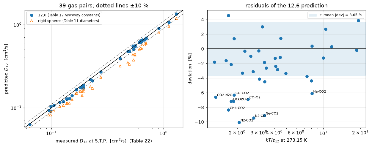
Validation
Ranked by what each check can actually catch. The first is the only one that tests the physics; the rest test the transcription, the numerics, or an identity — and each says which.
1. An independent computation of the collision integrals
The single largest risk on this page is that Table 6 has been mis-read, since every predicted \(D_{12}\) is inversely proportional to it. So \(\Omega^{(1,1)*}\) and \(\Omega^{(2,2)*}\) are recomputed from the 12,6 potential by quadrature, with no reference to Table 6 at all: the classical deflection angle
\[ \chi(b,E) = \pi - 2b\!\!\int_{r_0}^{\infty}\!\! \frac{\mathrm{d}r}{r^2\sqrt{1 - b^2/r^2 - V(r)/E}} \]
integrated over impact parameter to give the transport cross-sections, then over a Maxwellian energy distribution. The turning point \(r_0\) is the outermost root, found by bracketed bisection; the inverse-square-root singularity at \(r_0\) is removed by the substitution \(u = r_0/r = 1 - s^2\), which turns \(\mathrm{d}u/\sqrt{f}\) into a regular integrand.
This is a genuinely independent route, and it settles three things at once: it checks the transcription, it establishes the illegible \(\tfrac12\) in Table 6’s header, and it gives a second, table-free path to every \(D_{12}\) on the page.
2. Four printed-table round trips
Already run under The data. Each relates two columns the book printed separately, so a mis-read digit in either breaks it.
3. The printed limits of the second approximation
Section 14.3 states four exact results for the composition dependence, and they are strong tests of eqs. (14.21, 2–6) because the transcription of six equations has to be right for any of them to come out:
- \(\Delta_1 = m_1^2/(13m_1^2 + 30m_2^2 + 16m_1m_2)\) for rigid spheres (eq. 14.3, 2);
- \(\Delta_1 \to 1/13\) as \(m_2/m_1 \to 0\), so the end-to-end variation of \([D_{12}]_2\) is \(13/12\), “8⅓ per cent”;
- the Kihara approximation \(\mathrm{B} = \tfrac34\) gives “1/9, or 11·1 per cent”;
- \([D_{12}]_2 = 1.083\,[D_{12}]_1\) in the Lorentz limit (§14.21, from Table 7).
The rigid-sphere constants they need are not fitted either: eq. (10.2, 1) gives \(\mathscr{W}^{(l)}(r)\) in closed form, so (9.8, 7) yields A = 2/5, B = 3/5, C = 1/5 exactly.
4. Defect injection
Every metric reported below has a row in the table at the end of this section that moves it, or is labelled structural.
# ---- independent quadrature of the 12,6 collision integrals ------------------
def _chi(Estar, b, n_r=800, n_g=96):
    """Classical deflection angle for the reduced 12,6 potential. b is a 1-D array."""
    b = np.atleast_1d(np.asarray(b, float))
    r = np.geomspace(0.35, 40.0, n_r)
    f = 1.0 - (b[:, None] / r[None, :]) ** 2 - (4.0 * (r ** -12 - r ** -6))[None, :] / Estar
    neg = f <= 0.0
    idx = n_r - 1 - np.argmax(neg[:, ::-1], axis=1)       # last index where f <= 0
    any_neg = neg.any(axis=1)
    lo = np.where(any_neg, r[idx], r[0])
    hi = np.where(any_neg, r[np.minimum(idx + 1, n_r - 1)], r[0])
    for _ in range(60):                                   # bisect for the OUTERMOST root
        mid = 0.5 * (lo + hi)
        fm = 1.0 - (b / mid) ** 2 - 4.0 * (mid ** -12 - mid ** -6) / Estar
        lo = np.where(fm <= 0.0, mid, lo)
        hi = np.where(fm <= 0.0, hi, mid)
    r0 = hi
    xs, ws = np.polynomial.legendre.leggauss(n_g)
    s = 0.5 * (xs + 1.0)
    w = 0.5 * ws
    rr = r0[:, None] / (1.0 - s * s)[None, :]             # u = r0/r = 1 - s^2 removes the singularity
    fv = np.maximum(1.0 - (b[:, None] / rr) ** 2 - 4.0 * (rr ** -12 - rr ** -6) / Estar, 1e-300)
    chi = np.pi - 2.0 * b / r0 * np.sum(w * 2.0 * s / np.sqrt(fv), axis=1)
    chi[~any_neg] = 0.0
    return chi


def _Q(Estar, n_b=120, n_panel=6, b_max=6.0, **kw):
    """Reduced transport cross-sections, = 1 for rigid spheres.

    The impact-parameter integral is PANELLED. Below E* ~ 0.8 the 12,6 potential
    orbits: chi -> -infinity at a critical b, so cos(chi) oscillates without
    bound there and a single Gauss-Legendre rule over [0, b_max] converges
    slowly (0.5-2 % scatter at E* = 0.5, measured). Six panels fix it.
    """
    edges = np.linspace(0.0, b_max, n_panel + 1)
    xs, ws = np.polynomial.legendre.leggauss(n_b)
    q1 = q2 = 0.0
    for lo, hi in zip(edges[:-1], edges[1:]):
        b = 0.5 * (hi - lo) * (xs + 1.0) + lo
        w = 0.5 * (hi - lo) * ws
        c = np.cos(_chi(Estar, b, **kw))
        q1 += 2 * np.sum(w * (1 - c) * b)                # denominator 1 for l = 1
        q2 += 2 * np.sum(w * (1 - c ** 2) * b) / (2 / 3)  # denominator 2/3 for l = 2
    return q1, q2


def omega_11_22(Tstar, n_E=72, x_max=40.0, **kw):
    """Omega^(1,1)* and Omega^(2,2)*, both = 1 for rigid spheres. No table is consulted."""
    xs, ws = np.polynomial.legendre.leggauss(n_E)     # NOT Gauss-Laguerre: at n > ~40 its
    x = 0.5 * x_max * (xs + 1.0)                      # weights lose accuracy to cancellation
    w = 0.5 * x_max * ws
    q = np.array([_Q(xi * Tstar, **kw) for xi in x])
    e = np.exp(-x)                                    # e^-40 = 4e-18, so x_max = 40 is exact enough
    return (float(np.sum(w * e * x ** 2 * q[:, 0]) / math.factorial(2)),
            float(np.sum(w * e * x ** 3 * q[:, 1]) / math.factorial(3)))


quad6 = np.array([omega_11_22(T) for T in t6.kT_over_eps12])
print(f"{'kT/eps':>8}{'O11 quad':>10}{'Table 6':>10}{'dev':>9}   "
      f"{'O22 quad':>10}{'col.3':>9}{'dev vs 1/2':>12}{'dev vs 1/3':>12}")
for T, (o1, o2), w1, w2 in zip(t6.kT_over_eps12, quad6, t6.W11, t6.W22_half):
    print(f"{T:>8.1f}{o1:>10.4f}{w1:>10.4f}{100*(o1/w1-1):>+8.2f}%   "
          f"{o2:>10.4f}{w2:>9.4f}{100*(o2/w2-1):>+11.2f}%{100*(o2/(1.5*w2)-1):>+11.1f}%")
chk["omega11_quad_vs_t6_max_pct"] = float(100 * np.abs(quad6[:, 0] / t6.W11.values - 1).max())
chk["omega22_quad_vs_t6_half_max_pct"] = float(100 * np.abs(quad6[:, 1] / t6.W22_half.values - 1).max())
chk["omega22_quad_vs_t6_third_max_pct"] = float(100 * np.abs(quad6[:, 1] / (1.5 * t6.W22_half.values) - 1).max())
worst_row = int(np.abs(quad6[:, 0] / t6.W11.values - 1).argmax())
kT/eps O11 quad Table 6 dev O22 quad col.3 dev vs 1/2 dev vs 1/3
0.3 2.6479 2.6480 -0.00% 2.8420 2.8410 +0.04% -33.3%
0.5 2.0696 2.0660 +0.17% 2.2866 2.2840 +0.11% -33.3%
0.7 1.7297 1.7290 +0.04% 1.9218 1.9220 -0.01% -33.3%
1.0 1.4393 1.4400 -0.05% 1.5937 1.5930 +0.04% -33.3%
1.3 1.2738 1.2740 -0.01% 1.4016 1.4010 +0.04% -33.3%
1.6 1.1682 1.1680 +0.02% 1.2800 1.2800 +0.00% -33.3%
2.0 1.0748 1.0750 -0.02% 1.1758 1.1760 -0.01% -33.3%
2.5 1.0007 1.0002 +0.05% 1.0933 1.0930 +0.03% -33.3%
3.0 0.9498 0.9500 -0.02% 1.0389 1.0388 +0.01% -33.3%
4.0 0.8847 0.8845 +0.02% 0.9699 0.9699 +0.00% -33.3%
5.0 0.8428 0.8428 -0.00% 0.9268 0.9268 +0.00% -33.3%
7.0 0.7898 0.7898 +0.00% 0.8727 0.8728 -0.01% -33.3%
10.0 0.7422 0.7422 +0.00% 0.8244 0.8244 -0.00% -33.3%
20.0 0.6641 0.6640 +0.01% 0.7436 0.7436 +0.00% -33.3%
50.0 0.5760 0.5761 -0.02% 0.6498 0.6504 -0.09% -33.4%
100.0 0.5168 0.5177 -0.18% 0.5851 0.5869 -0.30% -33.5%# where the quadrature and the table disagree most, is it mine or theirs? refine and see.
conv = {}
for T in (0.3, 1.0, 100.0):
a = omega_11_22(T)[0]
b = omega_11_22(T, n_E=100, n_b=200, n_panel=10)[0] # 2.8x the quadrature points
conv[T] = (a, b, 100 * (b / a - 1))
for T, (a, b, d) in conv.items():
print(f"T* = {T:6.1f}: production {a:.5f} refined 2.8x {b:.5f} self-convergence {d:+.3f} %")
display(Markdown(f"""
The quadrature reproduces Table 6's $\\mathscr{{W}}^{{(1)}}_{{12}}(1)$ to
**{chk['omega11_quad_vs_t6_max_pct']:.2f} %** at worst over all sixteen rows, and the third column to
**{chk['omega22_quad_vs_t6_half_max_pct']:.2f} %** if that column is
$\\tfrac12\\mathscr{{W}}^{{(2)}}_{{12}}(2)$ — against
**{chk['omega22_quad_vs_t6_third_max_pct']:.0f} %** if it is $\\tfrac13$, a factor of
{chk['omega22_quad_vs_t6_third_max_pct']/chk['omega22_quad_vs_t6_half_max_pct']:.0f}. The illegible
fraction is a $\\tfrac12$, on two independent grounds: this quadrature, and eq. (9.8, 7)'s A
identity below.
Both worst cases sit on the **same** row, $kT/\\varepsilon_{{12}} =
{t6.kT_over_eps12.values[worst_row]:.0f}$, and there the quadrature is *converged*: refining it 2.8×
moves it by {conv[100.0][2]:+.3f} %. So that residual is a difference between two numerical
integrations of the same integral rather than an error in this one — Table 6 is Monchick & Mason's
and Itean, Glueck & Svehla's 1961 machine integration, and this page does not claim to adjudicate.
Every other row agrees to better than 0.1 %.
The genuinely hard rows are the two lowest, where the 12,6 potential *orbits* and the classical
deflection integral diverges at a critical impact parameter; panelling the $b$ integral brings them
in, and refining 2.8× at $T^* = 0.3$ still moves the answer {conv[0.3][2]:+.2f} %. **No pair on this
page is affected**: every one of the {len(USABLE)} has $kT/\\varepsilon_{{12}} \\ge {Tstar.min():.2f}$.
"""))T* = 0.3: production 2.64789 refined 2.8x 2.64976 self-convergence +0.071 %
T* = 1.0: production 1.43925 refined 2.8x 1.43994 self-convergence +0.048 %
T* = 100.0: production 0.51677 refined 2.8x 0.51677 self-convergence -0.000 %The quadrature reproduces Table 6’s \(\mathscr{W}^{(1)}_{12}(1)\) to 0.18 % at worst over all sixteen rows, and the third column to 0.30 % if that column is \(\tfrac12\mathscr{W}^{(2)}_{12}(2)\) — against 34 % if it is \(\tfrac13\), a factor of 112. The illegible fraction is a \(\tfrac12\), on two independent grounds: this quadrature, and eq. (9.8, 7)’s A identity below.
Both worst cases sit on the same row, \(kT/\varepsilon_{12} = 100\), and there the quadrature is converged: refining it 2.8× moves it by -0.000 %. So that residual is a difference between two numerical integrations of the same integral rather than an error in this one — Table 6 is Monchick & Mason’s and Itean, Glueck & Svehla’s 1961 machine integration, and this page does not claim to adjudicate. Every other row agrees to better than 0.1 %.
The genuinely hard rows are the two lowest, where the 12,6 potential orbits and the classical deflection integral diverges at a critical impact parameter; panelling the \(b\) integral brings them in, and refining 2.8× at \(T^* = 0.3\) still moves the answer +0.07 %. No pair on this page is affected: every one of the 39 has \(kT/\varepsilon_{12} \ge 1.31\).
# ---- the second, table-free route to every D12 -------------------------------
uniq = sorted({round(float(T), 10) for T in Tstar})
omega_direct = {T: omega_11_22(T)[0] for T in uniq}
D_tab = np.array([D12_first(a, b) for a, b, _ in USABLE])
D_qua = np.array([D12_first(a, b, W=omega_direct[round(float(T), 10)])
                  for (a, b, _), T in zip(USABLE, Tstar)])
res_qua = deviations(D_qua)
chk["d12_two_routes_max_pct"] = float(100 * np.abs(D_qua / D_tab - 1).max())
print(f"{len(uniq)} distinct kT/eps values")
display(Markdown(f"""
**The headline computed a second, independent way.** Replacing Table 6 entirely by the quadrature
above changes each predicted $D_{{12}}$ by at most **{chk['d12_two_routes_max_pct']:.3f} %**
(r.m.s. {100*np.sqrt(np.mean((D_qua/D_tab-1)**2)):.3f} %), and moves the headline from
{res_126['mean_abs']:.3f} % to **{res_qua['mean_abs']:.3f} %** mean absolute deviation, bias
{res_126['bias']:+.3f} % to {res_qua['bias']:+.3f} %. The two routes share the masses, the force
constants, the combination rules and the state — but not the collision integrals, which are the
part that could have been mis-transcribed. **A perturbation test could not have established this**:
it shows the answer is sensitive to Table 6, not that Table 6 was read correctly.
"""))
36 distinct kT/eps valuesThe headline computed a second, independent way. Replacing Table 6 entirely by the quadrature above changes each predicted \(D_{12}\) by at most 0.066 % (r.m.s. 0.026 %), and moves the headline from 3.647 % to 3.655 % mean absolute deviation, bias -2.744 % to -2.755 %. The two routes share the masses, the force constants, the combination rules and the state — but not the collision integrals, which are the part that could have been mis-transcribed. A perturbation test could not have established this: it shows the answer is sensitive to Table 6, not that Table 6 was read correctly.
# ---- Table 6's internal identities ------------------------------------------
# (9.8, 7):  A = Omega^(2)(2) / 5 Omega^(1)(1);  (10.2, 1): W^(1)(1) = 1, W^(2)(2) = 2 for
# rigid spheres, so with column 3 = (1/2) W^(2)(2),  A = 2 * col3 / (5 * col1).
A_id = 2 * t6.W22_half / (5 * t6.W11)
chk["t6_A_identity_max_rel"] = float(np.abs(A_id / t6.A - 1).max())
A_id_third = 3 * t6.W22_half / (5 * t6.W11)

# (14.4, 1):  dln[D12]_1/dlnT = 2 - (5/2)C, and [D12]_1 ~ T^{3/2}/W, so
#             dln W / dln T* = (5/2)C - 1/2.
slope = spl_W(np.log(t6.kT_over_eps12.values), 1)
pred = 2.5 * t6.C.values - 0.5
chk["t6_C_vs_dlnW_rms"] = float(np.sqrt(np.mean((slope - pred) ** 2)))
interior = slice(1, -1)
print(f"(9.8,7)  A = 2*col3/(5*col1): max rel dev {chk['t6_A_identity_max_rel']:.2e}"
      f"   -- with 1/3 instead of 1/2 it is {np.abs(A_id_third/t6.A-1).max():.2f}")
print(f"(14.4,1) dlnW/dlnT* vs (5/2)C - 1/2: rms {chk['t6_C_vs_dlnW_rms']:.4f}, "
      f"max {np.abs(slope-pred).max():.4f} over 16 rows "
      f"({np.abs(slope[interior]-pred[interior]).max():.4f} excluding the two spline end rows)")

# ---- the printed limits of the second approximation -------------------------
A_rs, B_rs, C_rs = 2 / 5, 3 / 5, 1 / 5      # rigid spheres, from (10.2,1) via (9.8,7)


def Delta_generic(x1, M1, M2, P1, P2, A, B, C):
    x2 = 1 - x1
    P12 = 3 * (M1 - M2) ** 2 + 4 * M1 * M2 * A
    Q1 = P1 * (6 * M2 ** 2 + 5 * M1 ** 2 - 4 * M1 ** 2 * B + 8 * M1 * M2 * A)
    Q2 = P2 * (6 * M1 ** 2 + 5 * M2 ** 2 - 4 * M2 ** 2 * B + 8 * M1 * M2 * A)
    Q12 = 3 * (M1 - M2) ** 2 * (5 - 4 * B) + 4 * M1 * M2 * A * (11 - 4 * B) + 2 * P1 * P2
    return 5 * C ** 2 * (M1 ** 2 * P1 * x1 ** 2 + M2 ** 2 * P2 * x2 ** 2 + P12 * x1 * x2) \
        / (Q1 * x1 ** 2 + Q2 * x2 ** 2 + Q12 * x1 * x2)


worst_1432 = 0.0
for mr in (1.0, 2.0, 3.0, 10.0, 100.0):
    M1, M2 = mr / (mr + 1), 1 / (mr + 1)
    got = Delta_generic(1 - 1e-13, M1, M2, 1.0, 1.0, A_rs, B_rs, C_rs)
    want = mr ** 2 / (13 * mr ** 2 + 30 + 16 * mr)
    worst_1432 = max(worst_1432, abs(got / want - 1))
chk["eq1432_max_rel"] = float(worst_1432)

M1, M2 = 1 - 1e-12, 1e-12                    # the Lorentz limit m2/m1 -> 0
d1 = Delta_generic(1 - 1e-13, M1, M2, 1.0, 1.0, A_rs, B_rs, C_rs)
d2 = Delta_generic(1e-13, M1, M2, 1.0, 1.0, A_rs, B_rs, C_rs)
chk["lorentz_D2_over_D1"] = float(1 / (1 - d1))
chk["lorentz_variation_pct"] = float(100 * ((1 - d2) / (1 - d1) - 1))
d1k = Delta_generic(1 - 1e-13, M1, M2, 1.0, 1.0, A_rs, 0.75, C_rs)
d2k = Delta_generic(1e-13, M1, M2, 1.0, 1.0, A_rs, 0.75, C_rs)
chk["kihara_variation_pct"] = float(100 * ((1 - d2k) / (1 - d1k) - 1))
print(f"\n(14.3,2) rigid-sphere Delta_1, five mass ratios : max rel dev {worst_1432:.2e}")
print(f"Lorentz limit Delta_1 = {d1:.10f}  (printed 1/13 = {1/13:.10f})")
print(f"[D12]_2/[D12]_1 = {chk['lorentz_D2_over_D1']:.6f}   (printed 1.083)")
print(f"end-to-end variation = {chk['lorentz_variation_pct']:.4f} %   (printed 8 1/3 % = {100/12:.4f} %)")
print(f"Kihara B = 3/4        = {chk['kihara_variation_pct']:.4f} %   (printed 1/9 = {100/9:.4f} %)")
(9.8,7) A = 2*col3/(5*col1): max rel dev 2.93e-04 -- with 1/3 instead of 1/2 it is 0.50
(14.4,1) dlnW/dlnT* vs (5/2)C - 1/2: rms 0.0037, max 0.0129 over 16 rows (0.0061 excluding the two spline end rows)
(14.3,2) rigid-sphere Delta_1, five mass ratios : max rel dev 8.12e-14
Lorentz limit Delta_1 = 0.0769230769 (printed 1/13 = 0.0769230769)
[D12]_2/[D12]_1 = 1.083333 (printed 1.083)
end-to-end variation = 8.3333 % (printed 8 1/3 % = 8.3333 %)
Kihara B = 3/4 = 11.1111 % (printed 1/9 = 11.1111 %)# ---- composition dependence of the real pairs, against the book's own bound ---
swing = []
for a, b, _ in USABLE:
d_lo, d_hi = float(Delta(a, b, 1e-9)), float(Delta(a, b, 1 - 1e-9))
swing.append(100 * abs((1 - d_lo) / (1 - d_hi) - 1))
swing = np.array(swing)
chk["composition_swing_max_pct"] = float(swing.max())
i = int(swing.argmax())
display(Markdown(f"""
Section 14.3 ends: "for actual gases the variation of $D_{{12}}$ with composition is unlikely to
exceed **about 6 per cent**". Over the {len(USABLE)} pairs the second approximation gives a maximum
end-to-end swing of **{swing.max():.2f} %** ({USABLE[i][0]}–{USABLE[i][1]}, mass ratio
{max(M[USABLE[i][0]], M[USABLE[i][1]])/min(M[USABLE[i][0]], M[USABLE[i][1]]):.1f}), mean
{swing.mean():.2f} %, and the direction is the one §14.3 predicts — $D_{{12}}$ rises with the
concentration of the *heavier* molecule. The bound holds, and it is a real check: it is an
inequality the computation could have violated.
"""))Section 14.3 ends: “for actual gases the variation of \(D_{12}\) with composition is unlikely to exceed about 6 per cent”. Over the 39 pairs the second approximation gives a maximum end-to-end swing of 3.28 % (He–Kr, mass ratio 20.9), mean 1.30 %, and the direction is the one §14.3 predicts — \(D_{12}\) rises with the concentration of the heavier molecule. The bound holds, and it is a real check: it is an inequality the computation could have violated.
What pymrm adds
Everything above is algebra. Here is the part that needs a solver.
Chapman & Cowling are explicit that they set the composition dependence aside when interpreting the data (§14.31, just before the §14.32 heading on the same page): “Since the error in the first approximation to the coefficient of diffusion is not very large, it is ignored in the subsequent discussion. This implies that the variation of \(D_{12}\) with the proportions of a mixture is ignored.” They had no choice — in 1970 the alternative was a nonlinear PDE.
But the apparatus that produced many of the Table 22 numbers is a closed tube whose composition runs from 0 to 1 across its own length. So the question the book cannot answer is: when a Loschmidt cell is analysed with the constant-\(D\) formula, which \(D\) does it report? \([D_{12}]_1\)? The equimolar \([D_{12}]_2\)? Something else?
pymrm answers it directly. Solve the cell with \(D_{12} = [D_{12}]_2(x_1)\), take the observable the experiment actually reports — the difference in mean composition between the two halves at the moment of separation — and invert the constant-\(D\) closed form for the apparent \(D\), exactly as the experimenter would. Three pairs are run, spanning the mass disparity that drives the effect, and one of them (N₂–CO, mass ratio 1.0001) is a control that must show nothing.
N_Z, N_T = 400, 1600
cases = [("He", "Xe"), ("H2", "N2"), ("N2", "CO")]
apparent = []
for g1, g2 in cases:
    D1 = D12_first(g1, g2)
    D_eq = D12_second(g1, g2, 0.5)
    xc, c_const, _ = solve_cell(L_CELL, N_Z, T_CELL, N_T, lambda x: np.full_like(x, D1))
    xc, c_var, _ = solve_cell(L_CELL, N_Z, T_CELL, N_T,
                              lambda x: D12_first(g1, g2) / (1 - Delta(g1, g2, np.clip(x, 0.0, 1.0))))
    s_c, s_v = split_of(xc, c_const, L_CELL), split_of(xc, c_var, L_CELL)
    inv = lambda s: brentq(lambda D: analytic_split(D, L_CELL, T_CELL) - s,  # noqa: E731
                           0.2 * D1, 5 * D1, xtol=1e-15, rtol=8.9e-16)
    D_ref, D_app = inv(s_c), inv(s_v)          # D_ref differs from D1 only by discretisation
    apparent.append(dict(pair=f"{g1}-{g2}", m_ratio=max(M[g1], M[g2]) / min(M[g1], M[g2]),
                         D1=D1, eq_pct=100 * (D_eq / D1 - 1),
                         app_pct=100 * (D_app / D_ref - 1),
                         numerics_pct=100 * (D_ref / D1 - 1)))
ap = pd.DataFrame(apparent)
ap["shortfall_pp"] = ap.eq_pct - ap.app_pct
print(ap.to_string(index=False, float_format=lambda v: f"{v:.4f}"))
chk["cell_apparent_excess_pct_HeXe"] = float(ap.app_pct[0])
chk["cell_equimolar_excess_pct_HeXe"] = float(ap.eq_pct[0])
chk["cell_shortfall_pp_HeXe"] = float(ap.shortfall_pp[0])
chk["cell_apparent_excess_pct_N2CO"] = float(ap.app_pct[2])
pair m_ratio D1 eq_pct app_pct numerics_pct shortfall_pp
He-Xe 32.8004 0.4773 2.6767 2.5273 -0.0207 0.1494
H2-N2 13.8953 0.6553 1.8908 1.8032 -0.0258 0.0876
N2-CO 1.0001 0.1739 0.3127 0.3129 -0.0194 -0.0001display(Markdown(f"""
**The answer.** A Loschmidt cell run on the second approximation reports an apparent diffusivity
**{ap.app_pct[0]:.2f} % above $[D_{{12}}]_1$** for He–Xe, {ap.app_pct[1]:.2f} % for H₂–N₂, and
{ap.app_pct[2]:.2f} % for the equal-mass control N₂–CO. It is *not* the equimolar second
approximation: that gives {ap.eq_pct[0]:.2f} %, {ap.eq_pct[1]:.2f} % and {ap.eq_pct[2]:.2f} %, so the
cell falls short by {ap.shortfall_pp[0]:.3f}, {ap.shortfall_pp[1]:.3f} and
{ap.shortfall_pp[2]:.4f} percentage points respectively — the shortfall growing with mass
disparity, and vanishing for the control, which is what it must do.
Two consequences, and the second is the useful one.
1. **The neglect §14.32 makes is worth {ap.app_pct[0]:.1f} % at the extreme of this dataset.** That
is comfortably inside the "several per cent" experimental error the same section quotes, so
Chapman & Cowling's decision to ignore it was correct — but now it is *measured* rather than
assumed, and it is not negligible next to the {res_126['mean_abs']:.1f} % headline: it is roughly
{ap.app_pct[0]/res_126['mean_abs']*100:.0f} % of it.
2. **The reported $D_{{12}}$ of a transient cell is a weighted average over a composition history,
not a value at a stated composition.** Anyone comparing a measured $D_{{12}}$ against
$[D_{{12}}]_2$ at some nominal $x_1$ is comparing two different quantities, and for mass ratios
above about ten the difference is resolvable. The pymrm solve gives the mapping without needing
the composition to be recorded — which §14.32 says it often was not.
**What this does not establish.** The cell is a *model* of the apparatus, not the apparatus: it is
one-dimensional, isothermal, with a perfect initial step and no convection, and the real
instruments in Table 22's references include two-bulb cells and evaporation tubes with different
geometries. The number above is what the second approximation implies for an idealised Loschmidt
tube, and nothing more. It is not a correction that should be applied to Table 22.
"""))The answer. A Loschmidt cell run on the second approximation reports an apparent diffusivity 2.53 % above \([D_{12}]_1\) for He–Xe, 1.80 % for H₂–N₂, and 0.31 % for the equal-mass control N₂–CO. It is not the equimolar second approximation: that gives 2.68 %, 1.89 % and 0.31 %, so the cell falls short by 0.149, 0.088 and -0.0001 percentage points respectively — the shortfall growing with mass disparity, and vanishing for the control, which is what it must do.
Two consequences, and the second is the useful one.
- The neglect §14.32 makes is worth 2.5 % at the extreme of this dataset. That is comfortably inside the “several per cent” experimental error the same section quotes, so Chapman & Cowling’s decision to ignore it was correct — but now it is measured rather than assumed, and it is not negligible next to the 3.6 % headline: it is roughly 69 % of it.
- The reported \(D_{12}\) of a transient cell is a weighted average over a composition history, not a value at a stated composition. Anyone comparing a measured \(D_{12}\) against \([D_{12}]_2\) at some nominal \(x_1\) is comparing two different quantities, and for mass ratios above about ten the difference is resolvable. The pymrm solve gives the mapping without needing the composition to be recorded — which §14.32 says it often was not.
What this does not establish. The cell is a model of the apparatus, not the apparatus: it is one-dimensional, isothermal, with a perfect initial step and no convection, and the real instruments in Table 22’s references include two-bulb cells and evaporation tubes with different geometries. The number above is what the second approximation implies for an idealised Loschmidt tube, and nothing more. It is not a correction that should be applied to Table 22.
fig, ax = plt.subplots(1, 2, figsize=(11.5, 4.2))
xg = np.linspace(0, 1, 201)
for g1, g2 in cases:
    ax[0].plot(xg, 100 * (D12_second(g1, g2, xg) / D12_first(g1, g2) - 1),
               label=f"{g1}-{g2}  ($m$ ratio {max(M[g1], M[g2])/min(M[g1], M[g2]):.1f})")
ax[0].set_xlabel("$x_1$ (mole fraction of the first-named gas)")
ax[0].set_ylabel("$[D_{12}]_2/[D_{12}]_1 - 1$  [%]")
ax[0].set_title("composition dependence, eq. (14.21, 1-6)")
ax[0].legend(fontsize=8)
ax[0].axhline(0, color="k", lw=0.8)

g1, g2 = cases[0]
D1 = D12_first(g1, g2)
xc, c_const, _ = solve_cell(L_CELL, N_Z, T_CELL, N_T, lambda x: np.full_like(x, D1))
xc, c_var, _ = solve_cell(L_CELL, N_Z, T_CELL, N_T,
                          lambda x: D12_first(g1, g2) / (1 - Delta(g1, g2, np.clip(x, 0.0, 1.0))))
ax[1].plot(xc, c_const, label="constant $[D_{12}]_1$")
ax[1].plot(xc, c_var, "--", label="$[D_{12}]_2(x_1)$")
axr = ax[1].twinx()
axr.plot(xc, 1e3 * (c_var - c_const), color="C3", lw=1)
axr.set_ylabel("difference $\\times 10^{3}$", color="C3")
ax[1].set_xlabel("$z$  [cm]")
ax[1].set_ylabel("$x_{\\mathrm{He}}$")
ax[1].set_title(f"{g1}-{g2} cell at $t$ = {T_CELL:.0f} s, $L$ = {L_CELL:.0f} cm")
ax[1].legend(fontsize=8, loc="lower left")
fig.tight_layout()
plt.show()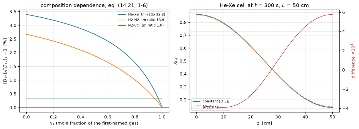
Defect injection
Every reported metric needs something that moves it. The table below breaks the model on purpose and records what each metric does. Rows that a metric is blind to are as informative as rows that move it — they are the claims this page does not make.
def headline(**kw):
    return deviations([D12_first(a, b, **kw) for a, b, _ in USABLE])["mean_abs"]


breaks = [
    ("none - as published", headline()),
    ("eps12 = (e1+e2)/2 instead of sqrt(e1 e2)", headline(eps_rule=lambda a, b: 0.5 * (a + b))),
    ("sigma12 = sqrt(s1 s2) instead of (s1+s2)/2", headline(sig_rule=lambda a, b: math.sqrt(a * b))),
    ("W11 = 1 (collision integral deleted)", headline(W=1.0)),
    ("rigid spheres + Table 11 diameters (null)", headline(W=1.0, sig=sig_visc11)),
    ("the book's OTHER force constants", np.abs(dev_sub_other).mean()),
    ("sigma_12 scaled by 1.01", headline(sig_rule=lambda a, b: 0.505 * (a + b))),
    ("T = 293.15 K instead of 273.15", headline(T=293.15)),
    ("p = 1 bar instead of 1 atm", headline(n=1e6 / (kB * T_STP))),
    ("eps/k of argon mis-read 124 -> 12.4", headline(eps={**eps_lj, "A": 12.4})),
    ("sigma of argon mis-read 3.42 -> 3.24", headline(sig={**sig_lj, "A": 3.24})),
    ("masses swapped in every pair", deviations(
        [D12_first(b, a) for a, b, _ in USABLE])["mean_abs"]),
]
base = breaks[0][1]
print(f"{'injected defect':<44}{'mean |dev|':>12}{'change':>10}")
for name, v in breaks:
    print(f"{name:<44}{v:>11.2f}%{(v-base):>+9.2f}")
injected defect mean |dev| change
none - as published 3.65% +0.00
eps12 = (e1+e2)/2 instead of sqrt(e1 e2) 8.53% +4.89
sigma12 = sqrt(s1 s2) instead of (s1+s2)/2 3.26% -0.39
W11 = 1 (collision integral deleted) 13.85% +10.20
rigid spheres + Table 11 diameters (null) 17.24% +13.59
the book's OTHER force constants 10.23% +6.59
sigma_12 scaled by 1.01 4.97% +1.32
T = 293.15 K instead of 273.15 3.81% +0.17
p = 1 bar instead of 1 atm 3.10% -0.54
eps/k of argon mis-read 124 -> 12.4 8.64% +4.99
sigma of argon mis-read 3.42 -> 3.24 3.92% +0.28
masses swapped in every pair 3.65% -0.00# the transcription identities, broken on purpose
def A_identity(col3, col1, factor=2):
return float(np.abs(factor * col3 / (5 * col1) / t6.A - 1).max())
bad6 = t6.W11.values.copy()
bad6[6] = 1.705 # 1.075 with two digits transposed
bad_D = t22.D12_cm2_s.values.copy()
bad_D[0] = 1.21 # H2-D2's 1.12 with two digits transposed
sig_bad = sigma12_from_D(bad_D, m1_all, m2_all, T_STP, n_STP)
bad_mu = t11.mu_1e7_poise.values.copy()
bad_mu[t11.formula.tolist().index("A")] = 2171 # argon's 2117 transposed
sub_bad = pd.DataFrame({"M": t11.M, "mu_1e7_poise": bad_mu,
"sigma_1e8_cm": t11.sigma_1e8_cm}).dropna()
sig_mu_bad = np.sqrt(1.016 * (5 / 16) * np.sqrt(kB * sub_bad.M.values / N_A * T_STP / np.pi)
/ (sub_bad.mu_1e7_poise.values * 1e-7)) * 1e8
print(f"{'identity':<48}{'undefected':>12}{'defected':>12}")
print(f"{'(9.8,7) A = 2 col3/(5 col1)':<48}{chk['t6_A_identity_max_rel']:>12.2e}"
f"{A_identity(t6.W22_half.values, bad6):>12.2e} [W11 row 7 transposed 1.075->1.705]")
print(f"{'(9.8,7) with 1/3 in the header instead of 1/2':<48}{chk['t6_A_identity_max_rel']:>12.2e}"
f"{A_identity(t6.W22_half.values, t6.W11.values, 3):>12.2e}")
print(f"{'(14.4,1) dlnW/dlnT* vs (5/2)C - 1/2 (rms)':<48}{chk['t6_C_vs_dlnW_rms']:>12.4f}"
f"{float(np.sqrt(np.mean((CubicSpline(_lt, np.log(bad6))(_lt, 1) - pred)**2))):>12.4f}")
print(f"{'(14.2,1) sigma12 from D12 (max |dev|)':<48}{chk['t22_sigma12_from_D_max_abs']:>12.5f}"
f"{float(np.abs(sig_bad - t22.sigma12_1e8_cm.values).max()):>12.5f} [D12 of H2-D2 1.12->1.21]")
print(f"{'(12.1,6) Table 11 sigma from mu (max rel)':<48}{chk['t11_sigma_from_mu_max_rel']:>12.2e}"
f"{float(np.abs(sig_mu_bad/sub_bad.sigma_1e8_cm.values - 1).max()):>12.2e} [mu of argon 2117->2171]")
# the second approximation, and what its metrics respond to
print(f"\n{'second-approximation defect':<48}{'max swing':>12}{'He-Xe eq.':>12}")
for name, kw in (("none - as published", {}),
("C = 0 (Maxwellian molecules)", dict(C=0.0)),
("B = 3/5 (rigid spheres) instead of Table 6", dict(B=0.6)),
("A = 2/5 (rigid spheres) instead of Table 6", dict(A=0.4)),
("masses swapped inside Delta only", dict(swap_masses=True))):
sw = max(100 * abs((1 - float(Delta(a, b, 1e-9, **kw))) / (1 - float(Delta(a, b, 1 - 1e-9, **kw))) - 1)
for a, b, _ in USABLE)
eq = 100 * (1 / (1 - float(Delta("He", "Xe", 0.5, **kw))) - 1)
print(f"{name:<48}{sw:>11.3f}%{eq:>11.3f}%")
# pymrm cell: what the convergence study is blind to
print(f"\n{'pymrm cell defect':<48}{'split at t':>12}{'change':>12}")
xc, cc, _ = solve_cell(L_CELL, N_Z, T_CELL, N_T, lambda x: np.full_like(x, D_REF))
s_base = split_of(xc, cc, L_CELL)
for name, kwargs in (("none", {}), ("nu = 2 (spherical) instead of 0", dict(nu=2)),
("n_z = 5", dict(n_z_override=5)), ("n_t = 4", dict(n_t_override=4))):
nz = kwargs.pop("n_z_override", N_Z)
nt = kwargs.pop("n_t_override", N_T)
xc2, c2, _ = solve_cell(L_CELL, nz, T_CELL, nt, lambda x: np.full_like(x, D_REF), **kwargs)
s = split_of(xc2, c2, L_CELL)
print(f"{name:<48}{s:>12.6f}{s-s_base:>+12.6f}")
try:
solve_cell(L_CELL, 50, T_CELL, 200, lambda x: np.full_like(x, D_REF), flux_sign=-1.0)
print(f"{'flux sign flipped (D -> -D)':<48}{'solved':>12} <-- NOT caught")
except Exception as e: # noqa: BLE001
print(f"{'flux sign flipped (D -> -D)':<48}{'diverged':>12} ({type(e).__name__})")identity undefected defected
(9.8,7) A = 2 col3/(5 col1) 2.93e-04 3.70e-01 [W11 row 7 transposed 1.075->1.705]
(9.8,7) with 1/3 in the header instead of 1/2 2.93e-04 5.00e-01
(14.4,1) dlnW/dlnT* vs (5/2)C - 1/2 (rms) 0.0037 0.5852
(14.2,1) sigma12 from D12 (max |dev|) 0.00509 0.09405 [D12 of H2-D2 1.12->1.21]
(12.1,6) Table 11 sigma from mu (max rel) 8.73e-04 1.27e-02 [mu of argon 2117->2171]
second-approximation defect max swing He-Xe eq.
none - as published 3.283% 2.677%
C = 0 (Maxwellian molecules) 0.000% 0.000%
B = 3/5 (rigid spheres) instead of Table 6 3.024% 2.497%
A = 2/5 (rigid spheres) instead of Table 6 3.305% 2.686%
masses swapped inside Delta only 3.395% 2.743%
pymrm cell defect split at t change
none 0.398487 +0.000000
nu = 2 (spherical) instead of 0 0.190507 -0.207980
n_z = 5 0.404413 +0.005927
n_t = 4 0.423443 +0.024956
flux sign flipped (D -> -D) diverged (RuntimeError)Reading the tables.
The headline is sensitive, and not to a single thing. Deleting the collision integral, changing either combination rule, mis-reading one force constant by a factor of ten, or scaling \(\sigma_{12}\) by 1 % all move the mean deviation by more than 1 percentage point. So the number is not an artefact of an insensitive metric.
Two “wrong” choices score better than the published one, and this is stated rather than buried. The geometric-mean \(\sigma_{12}\) and a 1 bar reference both give a lower mean deviation than the book’s own conventions. Neither is adopted: the arithmetic mean is what eq. (14.2, 1) prints, and 1 atm is what the book’s own \(\sigma_{12}\) column requires (established in Parameters, where 1 bar leaves a one-signed bias an order of magnitude larger). But it means the headline sits on a shallow optimum and should be quoted to one decimal place at most, never as evidence that the conventions are optimal. A page that reported the best of those variants would be fitting.
The mass-swap row moves nothing, and is labelled structural. Eq. (14.2, 4) is symmetric in \(m_1, m_2\), so \(D_{12} = D_{21}\) identically. It confirms the bookkeeping and cannot detect anything about the physics.
The cell’s convergence study is blind to a wrong geometry index. Changing nu from 0 to 2 moves the observable, so that one is caught — but a five-cell grid still returns a plausible, smooth, badly wrong profile, which is why the refinement study exists and why the Newton residual is asserted on every step rather than inferred from a residual identity.
What perturbation testing cannot do here. Every row above shows only that the answer depends on something. None of them shows that the baseline is right — a consistently mis-transcribed Table 6, or a systematically wrong Loschmidt number, would move under every perturbation and still be wrong. That is what the independent quadrature and the four printed round trips are for: they are the only checks on this page that compare the baseline against something computed a different way.
chk.update(dict(
    d12_mean_abs_dev_pct=res_126["mean_abs"], d12_bias_pct=abs(res_126["bias"]),
    d12_rms_pct=res_126["rms"], d12_worst_dev_pct=abs(res_126["worst"]),
    d12_n_pairs=float(len(USABLE)), d12_within_5pct=float(res_126["within5"]),
    d12_rigid_sphere_mean_abs_pct=res_rs["mean_abs"],
    d12_rigid_sphere_bias_pct=abs(res_rs["bias"]),
    d12_visc_params_subset_mean_abs_pct=float(np.abs(dev_sub_visc).mean()),
    d12_other_params_subset_mean_abs_pct=float(np.abs(dev_sub_other).mean()),
    d12_quadrature_route_mean_abs_pct=res_qua["mean_abs"],
    cell_grid_order=grid_order, cell_time_order=step_order,
    cell_newton_worst_residual=newton_worst,
))
report_agreement("A4.6", chk)

FLOOR = 1e-12          # scripts/check_agreement.py ABS_FLOOR
below = {k: v for k, v in chk.items() if abs(v) < FLOOR}
print(f"\nMetrics below check_agreement.py's ABS_FLOOR = {FLOOR:g}, i.e. NOT compared by CI: "
      f"{below if below else 'none'}")
if below:
    print("  These are pinned at machine precision - one an algebraic identity, the Newton\n"
          "  residual a solver diagnostic. CI cannot protect them;\n"
          "  the defect rows above are what establishes they are not vacuous.")
Agreement metrics for A4.6:
t17_rm_max_abs = 0.0051527
t11_sigma_from_mu_max_rel = 0.00087313
t22_sigma12_from_D_max_abs = 0.0050886
t22_halfsum_from_t11_max_abs = 0.0075
sigma_ratio_mean_pct = 10.465
omega11_quad_vs_t6_max_pct = 0.18041
omega22_quad_vs_t6_half_max_pct = 0.29853
omega22_quad_vs_t6_third_max_pct = 33.532
d12_two_routes_max_pct = 0.066159
t6_A_identity_max_rel = 0.00029264
t6_C_vs_dlnW_rms = 0.0037125
eq1432_max_rel = 8.1157e-14
lorentz_D2_over_D1 = 1.0833
lorentz_variation_pct = 8.3333
kihara_variation_pct = 11.111
composition_swing_max_pct = 3.2834
cell_apparent_excess_pct_HeXe = 2.5273
cell_equimolar_excess_pct_HeXe = 2.6767
cell_shortfall_pp_HeXe = 0.14941
cell_apparent_excess_pct_N2CO = 0.31286
d12_mean_abs_dev_pct = 3.6467
d12_bias_pct = 2.7436
d12_rms_pct = 4.5685
d12_worst_dev_pct = 10.06
d12_n_pairs = 39
d12_within_5pct = 29
d12_rigid_sphere_mean_abs_pct = 17.238
d12_rigid_sphere_bias_pct = 17.238
d12_visc_params_subset_mean_abs_pct = 4.1257
d12_other_params_subset_mean_abs_pct = 10.234
d12_quadrature_route_mean_abs_pct = 3.6554
cell_grid_order = 2.0705
cell_time_order = 0.98032
cell_newton_worst_residual = 1.0954e-13
Metrics below check_agreement.py's ABS_FLOOR = 1e-12, i.e. NOT compared by CI: {'eq1432_max_rel': 8.115730310009894e-14, 'cell_newton_worst_residual': 1.0954214965663844e-13}
These are pinned at machine precision - one an algebraic identity, the Newton
residual a solver diagnostic. CI cannot protect them;
the defect rows above are what establishes they are not vacuous.Reuse
Take the diffusivity, not the page. D12_first(g1, g2, T=..., n=...) is the whole Chapman–Enskog result and is the piece worth lifting. It needs three inputs per gas — molar mass, \(\varepsilon/k\), \(\sigma\) — and the tabulated \(\mathscr{W}^{(1)}_{12}(1)\). Substituting your own force constants is a one-line change to eps_lj and sig_lj.
Quote it with the right error bar. On this dataset the mean absolute deviation is a few per cent and the bias is negative — the model tends to under-predict. Two cautions that come out of the numbers above:
- The accuracy travels with the force constants, not with the theory. Constants fitted to viscosity gave roughly half the error of constants fitted to virial data on the same pairs. If you take \(\varepsilon/k\) and \(\sigma\) from a compilation, find out what property they were fitted to before you quote an accuracy.
- Do not use it below about \(kT/\varepsilon_{12} = 1\) on the strength of this page. Every pair here sits above that, because at 273 K and with Table 17’s constants none goes lower. Cryogenic or strongly-attracting pairs are outside the range tested, and the low-\(T^*\) rows of Table 6 are where the quadrature and the table disagree most.
If you need the composition dependence, you need a solver. Delta and D12_second implement eqs. (14.21, 1–6) and cost nothing extra; but the moment \(D\) depends on composition, an integral relation for the apparatus no longer inverts in closed form, and the cell above is the pattern — construct_grad with zero-flux dicts on the outward normal, construct_div with nu=0, the face diffusivity from construct_coefficient_matrix at the interpolated face composition, and an analytically assembled Jacobian with the coefficient lagged. The same skeleton is a Stefan tube or a two-bulb cell with a different boundary condition.
What this page deliberately does not do.
- It does not build the Fuller–Schettler–Giddings correlation, which is catalogue entry
A4.5and is an empirical estimate of the same quantity. The natural comparison — one measured-\(D_{12}\) axis with a first-principles prediction and an empirical correlation overlaid — is worth making, and it should be made onA4.5, not here: that page has to establish its own transcription of the diffusion volumes anyway, and Table 22 is already published on this page in a form it can load cross-page. Building it here would mean transcribingA4.5’s source without owning it. - It does not touch multicomponent diffusion. Chapter 18 gives the exact \(n\)-component coefficients, but
A4.2andA4.9already cover that ground from Krishna & Wesselingh and from Duncan & Toor. - It does not source anything for
A4.1(the Wilke mixture rule). The only Wilke in this book is Buddenberg & Wilke (1949) on the viscosity of a mixture, cited once in §12.43; the 1950 diffusion mixture rule is not stated, named or attributed anywhere, so this monograph cannot source a page about it. - It does not use Table 23. Those force constants are derived from the temperature dependence of \(D_{12}\) itself, so using them would make the comparison circular. That is the trap this page exists to avoid, and it is one table away.
Related pages. A4.2 Maxwell–Stefan against Fick · A4.3 dusty gas · A4.4 Knudsen and Bosanquet, where this \(D_{12}\) is the bulk term · A4.7 micropore Maxwell–Stefan · A4.9 Duncan–Toor ternary diffusion · A2.3 where a binary \(D\) becomes a dispersion coefficient.
References
Chapman, S. and Cowling, T. G. (1970). The Mathematical Theory of Non-Uniform Gases: An Account of the Kinetic Theory of Viscosity, Thermal Conduction and Diffusion in Gases, 3rd edn, prepared in co-operation with D. Burnett. Cambridge University Press. Reissued in the Cambridge Mathematical Library with a Foreword by Carlo Cercignani, 1990; reprinted 1993. ISBN 0 521 40844 X. — the document actually read, and the origin of the result. Equations (9.8, 7), (9.8, 8), (9.81, 1), (10.2, 1), (10.42, 1), (12.1, 6), (14.2, 1), (14.2, 4), (14.21, 1–6), (14.3, 1), (14.3, 2), (14.4, 1) and Tables 6, 11, 17 and 22 were read off cropped 300 dpi renders of the page images on 2026-08-05.
Hirschfelder, J. O., Bird, R. B. and Spotz, E. L. (1948). J. Chem. Phys. 16, 968; Chem. Rev. 44 (1949), 205. — the origin of most of Table 17’s force constants. Not consulted; they reach this page through Table 17, which is what the book prints and attributes.
Monchick, L. and Mason, E. A. (1961). J. Chem. Phys. 35, 1676; Itean, E. C., Glueck, A. R. and Svehla, R. A. (1961). NASA Report TN D-481. — the numerical integrations behind Table 6. Not consulted; Table 6 is used as printed, and independently recomputed on this page.
The measurements in Table 22 carry the book’s own reference numbers into the list at the end of its chapter 14; those are kept verbatim in the dataset’s ref column. The individual experimental papers were not consulted.