# Colab environment cell - no-op if pymrm is already installed
try:
    import pymrm
except ImportError:
%pip install -q pymrm pyyaml sympyKnudsen diffusion and the Bosanquet relation
sec:A
struct:S3
tier:T0
data:tier6
phase:gas
What happens when the pore is small enough that molecules hit the wall more often than each other — and exactly where the Bosanquet interpolation 1/D = 1/D_K + 1/D_AB is right, which is not where you would guess.
Knudsen diffusion and the Bosanquet relation
Catalog ID: A4.4 · Structure: S3 (scalar diffusion–reaction) · Tier: T0
Inside a catalyst pellet or a membrane, a molecule collides with other molecules and with the pore wall. Which collision dominates is set by the Knudsen number — mean free path over pore diameter — and the two limits have different physics: bulk diffusion couples the species to each other, Knudsen diffusion couples each species only to the wall.
The universal engineering closure is the Bosanquet relation, adding the two resistances in series,
\[ \frac{1}{D_{\mathrm{eff}}} = \frac{1}{D_{K}} + \frac{1}{D_{AB}} . \]
It is an interpolation, not an identity, and this page is about the difference. Krishna and Wesselingh’s 1997 review derives it as a special case of the dusty gas model, names it, states the three conditions it needs, and says flatly that it is “very restricted in its applicability” — without saying how wrong it gets, or where.
This page answers that. It reads the dusty-gas relations off the review’s printed pages, implements them in pymrm, and measures the Bosanquet error as a function of Knudsen number and flux ratio. The answer is not the obvious one: the error is worst in the bulk-diffusion limit and vanishes in the Knudsen limit — the interpolation is exact precisely where the Knudsen term dominates, and wrong where it does not matter that it is there.
Background
The mechanisms. The review distinguishes three transport mechanisms inside a porous particle (its Fig. 40): bulk or free-molecular diffusion, significant at large pore sizes and high pressure, “where molecule–molecule collisions dominate over molecule–wall collisions”; Knudsen diffusion, which “becomes predominant when the mean-free path of the molecular species is much larger than the pore diameter and hence molecule–wall collisions become important”; and surface diffusion of adsorbed species, dominant in micropores. The review is explicit that bulk and Knudsen diffusion “occur together and it is prudent to take both mechanisms into account rather than assume that one or other mechanism is ‘controlling’”.
Why an interpolation is needed at all. In the Knudsen limit each species moves independently: it exchanges momentum only with the wall, so its flux depends on its own partial-pressure gradient and on nothing else. In the bulk limit species exchange momentum with each other, so one species’ flux depends on every other species’ flux. Those are structurally different laws, and the transition between them is not a small correction — it is a change in what the flux is a function of. Bosanquet’s relation asserts that the two resistances simply add. Whether that is right turns out to depend entirely on what the other species is doing.
Scope, and what belongs elsewhere. This page is the scalar closure: S3, one effective diffusivity per species, the thing that goes into a Thiele modulus. The general \(n\)-component matrix form of the dusty gas model — the review’s eqs. (86)–(87), its ternary He/Ne/Ar comparison against the Remick & Geankoplis capillary measurements in Fig. 44, and the viscous-flow term — is catalogue entry A4.3 and is not built here. Everything below is binary, which is the setting in which the Bosanquet relation is stated and used. Bulk multicomponent diffusion with no wall is page A4.2, built from the same review; nothing on that page involves a pore.
The published model
Source, and which document each equation came from. The Knudsen and Bosanquet results are pre-DOI: Knudsen’s kinetic-theory treatment dates from 1909 and Bosanquet’s interpolation from a 1944 British wartime report (BR-507), neither of which is on disk or reachable. Neither was consulted. Every equation below was read from Krishna & Wesselingh (1997), which is on disk, prints all of them with attribution, and names the Bosanquet formula. Equation numbers throughout are that review’s. Each was read off a 600 dpi render of the printed page on 2026-08-01 — the PDF is an Acrobat 3.0 Capture OCR of a scan whose text layer is unreliable (it renders eq. (86)’s prefactor as \(c_t/RT\) where the page prints \(1/RT\), and eq. (109)’s stoichiometric subscript \(\nu_1\) as \(\nu_{1i}\)).
The dusty gas model (eq. 82). The pore wall is treated as a giant motionless pseudo-species — “dust” — and the Maxwell–Stefan equations are written for the \((n{+}1)\)-component mixture. Eliminating the dust gives, for \(i = 1,\dots,n\),
\[ -\frac{1}{RT}\nabla p_i \;=\; \sum_{j=1}^{n}\frac{x_j N_i - x_i N_j}{\mathrm{D}^e_{ij}} \;+\; \frac{N_i}{\mathrm{D}^e_{iM}} . \]
The first term is the familiar Maxwell–Stefan friction against the other species; the second is friction against the wall. \(\mathrm{D}^e_{ij}\) are the effective binary pair diffusivities, \(\mathrm{D}^e_{iM}\) the effective Knudsen diffusivities.
The porous matrix (eqs. 83–84): \(\mathrm{D}^e_{ij} = (\varepsilon/\tau)\, \mathrm{D}_{ij}\), with \(\tau = 1\) for a cylindrical pore.
The Knudsen diffusivity (eq. 85), attributed to Jackson (1977) and Mason & Malinauskas (1983):
\[ \mathrm{D}^e_{iM} = \frac{\varepsilon}{\tau}\,\frac{d_0}{3}\sqrt{\frac{8RT}{\pi M_i}} , \]
with \(d_0\) the pore diameter and, in the review’s own words, “the square-root term represents the velocity of motion” — the mean molecular speed \(\bar v_i\). So \(\mathrm{D}^e_{iM} = (\varepsilon/\tau)\,d_0\bar v_i/3\): proportional to pore size, independent of pressure, and scaling as \(\sqrt{T}\) and \(1/\sqrt{M_i}\).
What that implies (stated on p. 887): the \(\mathrm{D}^e_{ij}\) are inversely proportional to pressure and independent of pore size, so in the bulk-controlled regime the fluxes are independent of both; the \(\mathrm{D}^e_{iM}\) are independent of pressure and proportional to pore size, so in the Knudsen-controlled regime the fluxes are directly proportional to both. Two testable claims.
Graham’s law (eq. 107). Imposing \(\nabla p = 0\) on a gaseous mixture constrains the fluxes:
\[ \sum_{i=1}^{n} N_i \sqrt{M_i} = 0 \qquad (\nabla p = 0;\ \text{gaseous mixtures}). \]
The effective diffusivity (eqs. 108–109). Defining \(D_i\) by \(N_i = -D_i(\,c_i\nabla_{T,p}\mu_i/RT + c_i \bar V_i \nabla p / RT + \dots)\) — which for an ideal gas is exactly \(N_i = -D_i \nabla c_i\) — and eliminating \(\nabla p\) with the review’s eq. (105) gives, for species 1,
\[ \frac{1}{D_1} = \frac{1}{\mathrm{D}^e_{1M}} + \sum_{j=2}^{n}\frac{x_j}{\mathrm{D}^e_{1j}}\left(1 - \frac{x_1\nu_j}{x_j\nu_1}\right) \;-\; \underbrace{\alpha'_1 x_1 \frac{\mathrm{D}_{\rm visc}}{\mathrm{D}_{1M}} \frac{\sum_i (\nu_i/\nu_1)/\mathrm{D}^e_{iM}} {1 + \mathrm{D}_{\rm visc}\sum_i \alpha'_i x_i/\mathrm{D}^e_{iM}}}_{\text{viscous flow}} . \]
The \(\nu_i\) are the stoichiometric coefficients: for a heterogeneous reaction the flux ratios are fixed by the stoichiometry, \(N_j/N_1 = \nu_j/\nu_1\). The review’s comment on this expression is the heart of the case: “The effective diffusivity thus defined will be a strong function of the composition and also the flux ratios of all the species participating in say a chemical reaction within the pellet.” This page works at \(\mathrm{D}_{\rm visc} = 0\) throughout — no viscous flow — for which the review’s own remark is that “neglect of the viscous flow contribution … is not very serious; this result is typical (Haynes, 1978)”.
The Bosanquet formula (eq. 110). “For the special case of a (i) binary mixture, (ii) with no net change in the number of moles, and (iii) satisfying eq. (107), eq. (109) simplifies to”
\[ \frac{1}{D_1} = \frac{1}{\mathrm{D}^e_{1M}} + \frac{1}{\mathrm{D}^e_{12}}, \]
“a relation usually referred to as the Bosanquet formula. As noted above this formula is very restricted in its applicability.”
That is the whole specification, and it is unusually sharp: the review does not merely assert the interpolation, it prints the exact expression the interpolation approximates and the conditions under which the two coincide. Everything this page measures is the gap between eq. (109) and eq. (110).
| Symbol | Code | Meaning |
|---|---|---|
| \(\mathrm{D}^e_{iM}\) | knudsen_D, dam/dbm |
effective Knudsen diffusivity, eq. 85 |
| \(\mathrm{D}^e_{12}\) | dab |
effective binary pair diffusivity, eq. 83 |
| \([B^e]\) | Cell.b_matrix |
dusty-gas resistance matrix, eqs. 82/87 |
| \(D_1\) | Cell.d_scalar(...) |
scalar effective diffusivity, eq. 109 |
| \(D_{\rm Bos}\) | Cell.d_scalar(..., bosanquet=True) |
eq. 110 |
| \(\rho = -N_2/N_1\) | rho |
the flux ratio eq. 109 depends on |
| \(\mathrm{Kn}\) | kn |
\(\mathrm{D}^e_{12}/\mathrm{D}^e_{1M}\), see below |
Parameters and assumptions
The Knudsen number used here. The review never defines one. This page uses
\[ \mathrm{Kn} \;\equiv\; \frac{\mathrm{D}^e_{12}}{\mathrm{D}^e_{1M}}, \]
which is the ratio of the two resistances in the Bosanquet sum and is therefore the natural abscissa for everything below. It is proportional to the physical mean-free-path-over-diameter, and under the elementary kinetic-theory estimate \(\mathrm{D}_{12} = \bar v\lambda/3\) it equals it exactly, because eq. (85) already reads \(\mathrm{D}^e_{1M} = \bar v d_0/3\). \(\mathrm{Kn} \to 0\) is bulk control, \(\mathrm{Kn}\to\infty\) Knudsen control, and the two resistances are equal at \(\mathrm{Kn} = 1\).
Dimensionless working. Most results are reported in the groups \((\mathrm{Kn}, \rho, \phi)\) with concentrations scaled by the surface value and diffusivities by \(D_{\rm Bos}\). This is deliberate and follows B3.1: the review prints no pore sizes, porosities or rate constants for a reacting pellet, so inventing them would add nothing traceable. Where a dimensional number is wanted, the page uses the review’s own printed binary pair diffusivities from its worked example on p. 872 — 8.33, 6.8 and 1.68 ×10⁻⁵ m² s⁻¹ for the H₂/N₂/CO₂ pairs, which the review introduces as values that “can be estimated from the kinetic gas theory” for the Duncan & Toor (1962) system — loaded cross-page from the published A4.2 dataset. The review prints no temperature and no pressure beside them; the 35.2 °C and 1 atm at which they are used here are Duncan & Toor’s own experimental conditions, taken from page A4.9’s dataset sidecar, and they enter only through a mean molecular speed and a total concentration. No conclusion on this page depends on either, and that is measured rather than asserted: substituting \(T = 400\) K, and separately scaling the borrowed diffusivities by 1.3, moves 2 of the 40 metrics this page reports as results and leaves the other 38 bit-identical. The two that move are the exponent-recovery deviations of the p. 887 scaling check, the page’s only quantities read off a dimensional sweep; they shift by roughly 10–25 % and stay far below the 0.1 that would put the review’s stated exponents in doubt. Results item 5b prints the table. Also used: \(\varepsilon/\tau = 1\), which is eq. (84)’s printed \(\tau = 1\) (a straight cylindrical pore) together with an assumed \(\varepsilon = 1\), and standard molar masses.
Assumptions, all of them the review’s: isothermal ideal gas; no viscous flow (\(\mathrm{D}_{\rm visc} = 0\), so the third term of eq. 109 is dropped); no surface diffusion; a single pore size; and, in the reacting pellet, first-order kinetics in A and a steady state, so the flux ratio is fixed by the stoichiometry.
The two settings. The Bosanquet relation is used in two places, and its conditions fail differently in each:
| setting | flux ratio \(\rho = -N_2/N_1\) | which K&W condition fails |
|---|---|---|
| isobaric binary counter-diffusion cell | \(\sqrt{M_1/M_2}\) (eq. 107, Graham) | (ii), unless \(M_1 = M_2\) |
| pellet with \(A \to \nu_B B\) | \(\nu_B\) (stoichiometry) | (ii) and (iii), unless \(\nu_B = 1\) |
Conditions (ii) and (iii) are simultaneously satisfiable only when the two species have the same molar mass — equimolar counter-diffusion of unequal masses violates Graham’s law and therefore generates a pressure gradient. That is the sense in which the formula is “very restricted”.
import sys, urllib.request
from pathlib import Path

# Make shared/gallery_utils.py importable locally and on Colab
if not any("shared" in p for p in sys.path):
    local = Path.cwd()
    for _ in range(4):
        if (local / "shared" / "gallery_utils.py").is_file():
            sys.path.insert(0, str(local / "shared")); break
        local = local.parent
    else:
        url = ("https://raw.githubusercontent.com/computational-chemical-engineering/pymrm-gallery/"
               "main/shared/gallery_utils.py")
        urllib.request.urlretrieve(url, "gallery_utils.py")
        sys.path.insert(0, ".")

import numpy as np
import sympy as sp
import matplotlib.pyplot as plt
from IPython.display import Markdown, display
from pymrm import (construct_grad, construct_div, construct_boundary_value_matrices,
                   NumJac, newton)
from gallery_utils import load_data, load_meta, cite_data, report_agreement

PAGE = "A4.4-knudsen-bosanquet"
PAGE_A42 = "A4.2-maxwell-stefan-vs-fick"      # cross-page: the printed pair diffusivities
RGAS = 8.314462618                            # J/(mol K)
plt.rcParams.update({"figure.dpi": 110, "axes.grid": True, "grid.alpha": 0.3})
np.seterr(all="ignore")
{'divide': 'warn', 'over': 'warn', 'under': 'ignore', 'invalid': 'warn'}The data
There is no dataset here in the experimental sense. This page is tier 6. Two collections of printed numbers are used, and neither is a measurement:
krishna-wesselingh-1997-porous-media.csv— the constants and stated results of the review’s dusty-gas sections (pp. 886–893), read off 600 dpi renders: the \(d_0/3\) and \(M^{-1/2}\) of eq. (85), \(\tau = 1\) of eq. (84), the \(\sqrt{M_i}\) of Graham’s law, and the review’s quotation of Jackson’s pellet-centre pressure with its “40 % increase” for \(\nu_B = 2\).- The review’s own binary pair diffusivities (p. 872), loaded cross-page from the published
A4.2dataset — 8.33, 6.8 and 1.68 ×10⁻⁵ m² s⁻¹ for the H₂/N₂/CO₂ pairs, which the review gives as estimates “from the kinetic gas theory” for the Duncan & Toor (1962) system and prints with no temperature and no pressure. Nothing was re-transcribed. The 35.2 °C and 1 atm at which they are used below come fromA4.9’s Duncan & Toor sidecar, not from this review.A4.2, which publishes this dataset, records that these three values are not measurements — Krishna & Wesselingh call them kinetic-theory estimates, Duncan & Toor call them the best literature values corrected to their thermostat temperature — and this page makes no experimental claim on them either. What they are worth here is measured in Results item 5b rather than assumed.
The review does contain a comparison with measurement — its Fig. 44, the dusty gas model against Remick & Geankoplis’s (1974) He/Ne/Ar capillary data. That comparison is ternary, needs figure digitisation, and belongs to A4.3. The conditions printed inside that figure are recorded in the sidecar for whoever builds it; the measured points are not, and this page makes no experimental claim.
pm = load_data("krishna-wesselingh-1997-porous-media.csv", page=PAGE)
pm_meta = load_meta("krishna-wesselingh-1997-porous-media.csv", page=PAGE)
P = {(r.group, r.symbol): r.value for r in pm.itertuples()}

wx = load_data("krishna-wesselingh-1997-worked-examples.csv", page=PAGE_A42)
wx_meta = load_meta("krishna-wesselingh-1997-worked-examples.csv", page=PAGE_A42)
W = {(r.example, r.symbol): r.value for r in wx.itertuples()}

print("page dataset :", cite_data(pm_meta))
print("cross-page   :", cite_data(wx_meta))
print(f"\n{len(pm)} printed constants and stated results; "
      f"{sum(1 for k in W if k[0] == 'ideal' and k[1].startswith('D'))} "
      f"pair diffusivities reused from A4.2")

# --- the review's own system, for the one dimensional illustration -----------
# K&W print these three pair diffusivities on p. 872 for the hydrogen/nitrogen/
# carbon dioxide system of Duncan & Toor (1962), as values that "can be
# estimated from the kinetic gas theory" - and they print NO temperature and NO
# pressure with them.  The 35.2 C and 1 atm below are Duncan & Toor's own
# experimental conditions, taken from page A4.9's dataset sidecar, NOT from this
# review.  They only set a mean molecular speed and a total concentration.  No
# CONCLUSION on this page depends on either, and Results item 5b measures
# what that is worth: T -> 400 K and D x 1.3 each move exactly 2 of the 40
# result metrics - the two exponent-recovery deviations of the p. 887 scaling
# check, which are read off a dimensional sweep - and leave the other 38
# bit-identical.  (The test itself contributes four further metrics, which are
# the perturbed values.)
T_REV = 308.35                       # K = 35.2 C  (Duncan & Toor's bath, via A4.9)
P_ATM = 101325.0                     # Pa          (Duncan & Toor's cell, via A4.9)
D_AB = {"H2-N2": W[("ideal", "D12")], "H2-CO2": W[("ideal", "D13")],
        "N2-CO2": W[("ideal", "D23")]}                       # m2/s, K&W p. 872
MOLAR = {"H2": 2.01588e-3, "N2": 28.0134e-3, "CO2": 44.0095e-3}   # kg/mol, IUPAC
TAU_CYL = P[("eq84", "tau_cylindrical")]     # eq. (84): tau = 1, cylindrical pore
EPS_POROSITY = 1.0                           # ASSUMED, not printed: one straight
                                             # open pore, so eps = 1
EPS_TAU = EPS_POROSITY / TAU_CYL             # the eps/tau factor of eqs. (83), (85)
KN_DEN = P[("eq85", "knudsen_denominator")]                  # eq. (85): d_0/3
KN_EXP = P[("eq85", "knudsen_mass_exponent")]                # eq. (85): M^-1/2
GR_EXP = P[("eq107", "graham_mass_exponent")]                # eq. (107): sqrt(M)
NU_B_PRINTED = P[("jackson", "nu_b_example")]                # nu_B = 2
DP_PRINTED = P[("jackson", "centre_pressure_increase")]      # "a 40% increase"
for k, v in D_AB.items():
    print(f"  D_{k:8s} = {v:.3e} m2/s   (K&W p. 872, kinetic gas theory; the "
          f"T and p at which they are used here come from A4.9)")
print(f"  eps/tau = {EPS_TAU:.1f}  (tau = {TAU_CYL:.0f} printed in eq. 84; "
      f"eps = {EPS_POROSITY:.0f} assumed, not printed)")
page dataset : Krishna, R.; Wesselingh, J. A. (1997) — Chemical Engineering Science 52(6) 861-911 — doi:10.1016/S0009-2509(96)00458-7 — table
cross-page : Krishna, R.; Wesselingh, J. A. (1997) — Chemical Engineering Science 52(6) 861-911 — doi:10.1016/S0009-2509(96)00458-7 — table
14 printed constants and stated results; 7 pair diffusivities reused from A4.2
D_H2-N2 = 8.330e-05 m2/s (K&W p. 872, kinetic gas theory; the T and p at which they are used here come from A4.9)
D_H2-CO2 = 6.800e-05 m2/s (K&W p. 872, kinetic gas theory; the T and p at which they are used here come from A4.9)
D_N2-CO2 = 1.680e-05 m2/s (K&W p. 872, kinetic gas theory; the T and p at which they are used here come from A4.9)
eps/tau = 1.0 (tau = 1 printed in eq. 84; eps = 1 assumed, not printed)PyMRM implementation
The Knudsen diffusivity, eq. (85)
One line, and the only place a molar mass enters.
def knudsen_D(d0, T, M, eps_tau=EPS_TAU):
    """K&W eq. (85): D^e_iM = (eps/tau)(d_0/3) sqrt(8 R T / (pi M_i)).

    d0 is the pore DIAMETER (the review's d_0), not the radius; the
    square-root term is the mean molecular speed, which the review names in
    the text as 'the velocity of motion'.
    """
    return eps_tau * (d0 / KN_DEN) * np.sqrt(8.0 * RGAS * T / np.pi) * M ** KN_EXP


for g, M in MOLAR.items():
    print(f"  {g:4s}  v_bar = {np.sqrt(8*RGAS*T_REV/(np.pi*M)):7.1f} m/s   "
          f"D_K(d0 = 100 nm) = {knudsen_D(100e-9, T_REV, M):.3e} m2/s")

# Where the two resistances are equal: D_K(d0) = D_AB.  This is the pore size
# at which Kn = 1, and (since eq. 85 gives D_K = v_bar d0/3) it is also the
# elementary kinetic-theory mean free path 3 D_AB / v_bar.
D0_CROSS = {}
for pair, dab in D_AB.items():
    a = pair.split("-")[0]
    D0_CROSS[pair] = KN_DEN * dab / np.sqrt(8 * RGAS * T_REV / (np.pi * MOLAR[a]))
    print(f"  Kn = 1 for {a:3s} in {pair:8s}: d_0 = {D0_CROSS[pair]*1e9:5.1f} nm")
H2 v_bar = 1799.6 m/s D_K(d0 = 100 nm) = 5.999e-05 m2/s
N2 v_bar = 482.8 m/s D_K(d0 = 100 nm) = 1.609e-05 m2/s
CO2 v_bar = 385.2 m/s D_K(d0 = 100 nm) = 1.284e-05 m2/s
Kn = 1 for H2 in H2-N2 : d_0 = 138.9 nm
Kn = 1 for H2 in H2-CO2 : d_0 = 113.4 nm
Kn = 1 for N2 in N2-CO2 : d_0 = 104.4 nm# --- eq. (85) scaling, and the transition curve ------------------------------
sT = knudsen_D(1e-7, 4 * T_REV, MOLAR["H2"]) / knudsen_D(1e-7, T_REV, MOLAR["H2"])
sM = knudsen_D(1e-7, T_REV, 4 * MOLAR["H2"]) / knudsen_D(1e-7, T_REV, MOLAR["H2"])
sD = knudsen_D(4e-7, T_REV, MOLAR["H2"]) / knudsen_D(1e-7, T_REV, MOLAR["H2"])
SCALE_DEV = max(abs(sT - 2.0), abs(sM - 0.5), abs(sD - 4.0))
d0s = np.logspace(-9, -4, 400)
fig, ax = plt.subplots(figsize=(7.0, 4.4))
for pair, dab in D_AB.items():
a = pair.split("-")[0]
dk = knudsen_D(d0s, T_REV, MOLAR[a])
ax.loglog(d0s * 1e9, 1.0 / (1.0 / dk + 1.0 / dab) / dab, lw=2,
label=f"{a} in {pair}")
ax.plot([D0_CROSS[pair] * 1e9], [0.5], "o", ms=6, color="k", zorder=5)
ax.loglog(d0s * 1e9, np.minimum(knudsen_D(d0s, T_REV, MOLAR["H2"]) / D_AB["H2-N2"], 1.0),
"k--", lw=1, label="asymptotes (H$_2$ in H$_2$-N$_2$)")
ax.set_xlabel("pore diameter $d_0$ / nm")
ax.set_ylabel(r"$D_{\rm Bos}\,/\,\mathrm{D}^e_{12}$")
ax.set_title(r"Bosanquet interpolation, eq. (110), for K&W's p. 872 pair "
r"diffusivities" "\n"
r"at 1 atm, 35.2 $^\circ$C (Duncan & Toor's conditions; K&W print "
r"none); $\bullet$ = $\mathrm{Kn}=1$")
ax.legend(fontsize=8, loc="lower right"); ax.set_ylim(1e-3, 2)
plt.tight_layout(); plt.show()
print(f"eq. (85) scalings: D_K(4T)/D_K(T) = {sT:.12f} (2), "
f"D_K(4M)/D_K(M) = {sM:.12f} (0.5), D_K(4d0)/D_K(d0) = {sD:.12f} (4)")
print(f"worst deviation from the exponents printed in eq. (85): {SCALE_DEV:.2e}")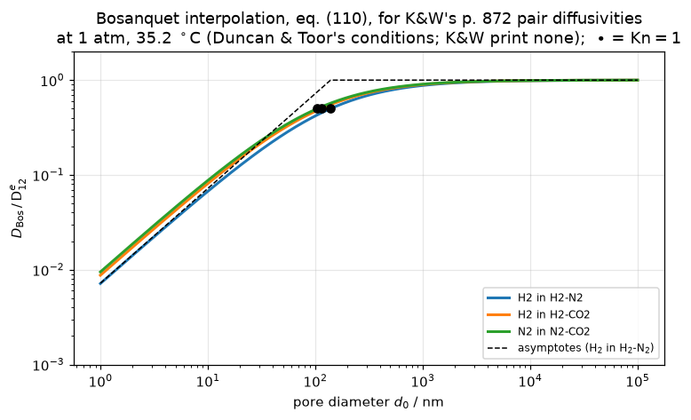
eq. (85) scalings: D_K(4T)/D_K(T) = 2.000000000000 (2), D_K(4M)/D_K(M) = 0.500000000000 (0.5), D_K(4d0)/D_K(d0) = 4.000000000000 (4)
worst deviation from the exponents printed in eq. (85): 0.00e+00
Eq. (109) checked against eq. (82), symbolically
Eq. (109) is the equation everything on this page rests on, it was read once off a scan, and its stoichiometric subscripts are exactly what the OCR mangles. So it is derived independently, from eq. (82), before being used — the B3.1 pattern: a transcription you can only read once should be checked against something you can derive.
For a binary mixture with flux ratio \(N_2/N_1 = -\rho\), eq. (82) for species 1 reads \(-\nabla c_1 = (x_2 N_1 - x_1 N_2)/\mathrm{D}^e_{12} + N_1/\mathrm{D}^e_{1M}\) (ideal gas, so \(\nabla p_1 = RT\nabla c_1\)), and solving it for \(D_1 = -N_1/\nabla c_1\) must reproduce eq. (109) with \(\mathrm{D}_{\rm visc} = 0\). Setting \(\rho = 1\) must then give eq. (110).
_NA, _xa, _xb, _dab, _dam, _dbm, _rho, _kn = sp.symbols(
    "N_A x_A x_B D_AB D_AM D_BM rho Kn", positive=True)

# eq. (82), species 1 of a binary, with N_2 = -rho N_1
_row = (_xb * _NA - _xa * (-_rho * _NA)) / _dab + _NA / _dam
_from82 = sp.simplify(sp.expand(_row / _NA))                  # = 1/D_1
_eq109 = 1 / _dam + (_xb / _dab) * (1 + _rho * _xa / _xb)     # eq. (109), D_visc = 0
EQ109_RESID = sp.simplify(_from82 - _eq109)

_eq110 = sp.simplify(_eq109.subs(_rho, 1).subs(_xb, 1 - _xa))
EQ110_RESID = sp.simplify(_eq110 - (1 / _dam + 1 / _dab))

# The Bosanquet error in closed form.  Scaling by D_bos makes 1/D_AM + 1/D_AB = 1,
# with D_AM/D_bos = 1 + 1/Kn and D_AB/D_bos = 1 + Kn.
_scaled = {_dam: 1 + 1 / _kn, _dab: 1 + _kn}
_ratio = sp.simplify((_eq109 / (1 / _dam + 1 / _dab)).subs(_xb, 1 - _xa).subs(_scaled))
ERR_RESID = sp.simplify(_ratio - (1 + (_rho - 1) * _xa / (1 + _kn)))

# K&W condition (iii).  The viscous term of eq. (109) carries the factor
# sum_i (nu_i/nu_1)/D^e_iM = 1/D_AM - rho/D_BM.  Solve for the rho that kills
# it: eq. (85) makes D_BM/D_AM = sqrt(M_A/M_B), which is exactly the flux ratio
# Graham's law (eq. 107) imposes.  So condition (iii) IS "the viscous term
# vanishes", and it coincides with condition (ii), rho = 1, only when the two
# molar masses are equal.
VISC_FACTOR = sp.simplify(1 / _dam - _rho / _dbm)
RHO_NO_VISC = sp.solve(sp.Eq(VISC_FACTOR, 0), _rho)[0]
VISC_AT_RHO1 = sp.simplify(VISC_FACTOR.subs(_rho, 1))

print("1/D_1 from eq. (82)      :", sp.nsimplify(_from82))
print("eq. (109), D_visc = 0    :", sp.expand(_eq109))
print("difference               :", EQ109_RESID)
print("eq. (109) at rho = 1     :", _eq110, " -> eq. (110) residual:", EQ110_RESID)
print("D_Bos/D_1 (scaled)       :", sp.simplify(_ratio),
      "  == 1 + (rho-1) x_A/(1+Kn), residual:", ERR_RESID)
print("viscous factor              :", VISC_FACTOR)
print("   vanishes at rho =        :", RHO_NO_VISC,
      " = sqrt(M_A/M_B), i.e. exactly Graham's law, eq. (107) = condition (iii)")
print("   its value at rho = 1     :", VISC_AT_RHO1,
      " -> zero only if M_A = M_B")
1/D_1 from eq. (82) : (D_AB + D_AM*(rho*x_A + x_B))/(D_AB*D_AM)
eq. (109), D_visc = 0 : 1/D_AM + rho*x_A/D_AB + x_B/D_AB
difference : 0
eq. (109) at rho = 1 : (D_AB + D_AM)/(D_AB*D_AM) -> eq. (110) residual: 0
D_Bos/D_1 (scaled) : (Kn + rho*x_A - x_A + 1)/(Kn + 1) == 1 + (rho-1) x_A/(1+Kn), residual: 0
viscous factor : -rho/D_BM + 1/D_AM
vanishes at rho = : D_BM/D_AM = sqrt(M_A/M_B), i.e. exactly Graham's law, eq. (107) = condition (iii)
its value at rho = 1 : (-D_AM + D_BM)/(D_AM*D_BM) -> zero only if M_A = M_BWhat that settles, and what it does not. Eq. (109) as transcribed is eq. (82) rearranged — the residual is identically zero — and it collapses to eq. (110) exactly when \(\rho = 1\), which is the review’s condition (ii). The transcription is therefore not in doubt. It also gives a closed form for the whole question this page asks:
\[ \boxed{\;\frac{D_{\rm Bos}}{D_1} \;=\; 1 + \frac{(\rho - 1)\,x_1}{1 + \mathrm{Kn}}\;} \]
The Bosanquet relation is exact when \(\rho = 1\), for any Knudsen number; its error grows linearly in the flux-ratio departure \(\rho - 1\) and in the mole fraction of the species itself; and — the part that is not obvious — it decays as \(1/(1+\mathrm{Kn})\), so it is largest in the bulk-diffusion limit and vanishes under Knudsen control. That is a statement about the physics, not about the algebra: under Knudsen control species do not exchange momentum with each other at all, so what the other species is doing cannot matter, and any formula that ignores the flux ratio is automatically right.
The last two symbolic lines identify the review’s condition (iii). The viscous term of eq. (109) carries the factor \(\sum_i(\nu_i/\nu_1)/\mathrm{D}^e_{iM} = 1/\mathrm{D}^e_{1M} - \rho/\mathrm{D}^e_{2M}\), and solving for the \(\rho\) that kills it gives \(\rho = \mathrm{D}^e_{2M}/\mathrm{D}^e_{1M} = \sqrt{M_1/M_2}\) — which is precisely the flux ratio Graham’s law imposes. Condition (iii) is exactly “the viscous term vanishes”. At \(\rho = 1\) that factor is \(1/\mathrm{D}^e_{1M} - 1/\mathrm{D}^e_{2M}\), so conditions (ii) and (iii) are two separate conditions and they close simultaneously only when \(M_1 = M_2\).
This is algebra, and it is labelled as algebra. It cannot detect an error in the pymrm assembly, in the boundary conditions, or in the discretisation. Everything below is there to test those.
The solver
One skeleton, three flux closures, following the A4.2 pattern:
dgm— the dusty gas model as eq. (82) stands: build the \(2\times2\) matrix \([B^e]\) of eq. (87) at every face from the local composition and solve \((N) = -[B^e]^{-1}(\nabla c)\), which is eq. (86) for an ideal gas. Nothing about the flux ratio is assumed — it comes out of the solve.eq109— the scalar effective diffusivity of eq. (109), with the flux ratio \(\rho\) prescribed. Diagonal: each species responds to its own gradient only.bosanquet— eq. (110), the same but with \(\rho\) forced to 1, so the diffusivities are constants.
The three routes differ only in the constitutive closure — they share the face reconstruction, both operators, the residual assembly and the same NumJac, and only the body of flux changes. That is exactly what their comparison can and cannot do: the scalar closures presume a flux ratio and dgm does not, so comparing them tests the presumption; it cannot see a discretisation error, because a wrong grid moves both routes together.
pymrm conventions, all of which matter here:
- Layout
(n, 2)— spatial axis first, species last. Not(n,)with the species stacked:NumJaccouples the last axis in full, so the field axis must be last or the stencil declares every cell coupled to every other. NumJac(shape, axes_diagonals=[0], axes_blocks=[-1])— the residual in a cell reads its neighbours through the face fluxes (axes_diagonals=[0], meaningful here becausendims = 2) and the two species couple pointwise through \([B^e]\) (axes_blocks=[-1]).- Boundary conditions on the OUTWARD normal. At a pellet centre the outward normal points inward, so symmetry is
{a:1, b:0, d:0}; a fixed external composition is{a:0, b:1, d:c_bnd}. Each carries its physical equation in a comment. nuinconstruct_divis geometry:0slab,1cylinder,2sphere. It is swept below, because one of the results turns out to be blind to it and that has to be said.- Constant operators are built once in
__init__; only the composition- dependent flux is recomputed.
class Cell:
    """Binary porous medium in 1-D, fields (n, 2) = (c_A, c_B).

    Dimensionless unless dimensional diffusivities and boundary
    concentrations are passed in.  `phi` switches on a first-order
    heterogeneous reaction A -> nu_B B distributed through the pellet.
    """

    def __init__(self, n=200, geom=0, bc_left=None, bc_right=None,
                 dam=1.0, dbm=1.0, dab=1.0, phi=0.0, nu_b=1.0,
                 model="dgm", rho=None, b_offdiag=1.0):
        self.n, self.geom, self.shape = n, geom, (n, 2)
        self.dam, self.dbm, self.dab = dam, dbm, dab      # D^e_AM, D^e_BM, D^e_AB
        self.phi, self.nu_b, self.model = phi, nu_b, model
        self.rho = nu_b if rho is None else rho           # flux ratio -N_B/N_A
        # Sign of the [B^e] off-diagonals, i.e. of the friction terms of eq. (82).
        # +1 is the printed equation; -1 is the deliberate defect injected in V3.
        self.b_offdiag = b_offdiag
        self.x_f = np.linspace(0.0, 1.0, n + 1)
        self.x_c = 0.5 * (self.x_f[:-1] + self.x_f[1:])
        # bc on the OUTWARD normal, a dc/dn + b c = d.  Callers pass, at a
        # pellet centre, {a:1,b:0,d:0} (symmetry, dc/dn = 0) and at an outer
        # face {a:0,b:1,d:c_bnd} (imposed external concentration).
        self.grad, gb = construct_grad(self.shape, self.x_f, self.x_c,
                                       (bc_left, bc_right))
        self.grad_bc = np.asarray(gb.todense()).reshape((-1, 1))
        self.div = construct_div(self.shape, self.x_f, nu=geom)   # 0 slab 1 cyl 2 sph
        bl, blb = construct_boundary_value_matrices(
            self.shape, self.x_f, self.x_c, bc_left, bound_id=0)
        br, brb = construct_boundary_value_matrices(
            self.shape, self.x_f, self.x_c, bc_right, bound_id=1)
        self.bval = (bl, np.asarray(blb.todense()).reshape(-1),
                     br, np.asarray(brb.todense()).reshape(-1))
        # last axis = species (pointwise coupling through [B^e]); axis 0 = space,
        # whose neighbours the face fluxes read.  ndims = 2, so axes_diagonals
        # is meaningful; on a bare 1-D shape it would not be.
        self.numjac = NumJac(self.shape, axes_diagonals=[0], axes_blocks=[-1])

    # ---------------------------------------------------------------- helpers
    def faces(self, c):
        """Face values and face gradients of (c_A, c_B)."""
        bl, blb, br, brb = self.bval
        cf = np.empty((self.n + 1, 2))
        cf[1:-1] = 0.5 * (c[:-1] + c[1:])
        cf[0] = (bl @ c.reshape((-1, 1))).ravel() + blb
        cf[-1] = (br @ c.reshape((-1, 1))).ravel() + brb
        g = (self.grad @ c.reshape((-1, 1)) + self.grad_bc).reshape(self.n + 1, 2)
        return cf, g

    def b_matrix(self, xf):
        """[B^e] of K&W eq. (87) for n = 2.  B_ii = 1/D_iM + sum_k!=i x_k/D_ik,
        B_ij = -x_i/D_ij."""
        xa, xb = xf[:, 0], xf[:, 1]
        b = np.empty(xf.shape[:-1] + (2, 2))
        b[..., 0, 0] = 1.0 / self.dam + xb / self.dab
        b[..., 0, 1] = -self.b_offdiag * xa / self.dab
        b[..., 1, 0] = -self.b_offdiag * xb / self.dab
        b[..., 1, 1] = 1.0 / self.dbm + xa / self.dab
        return b

    def d_scalar(self, xf, bosanquet=False):
        """K&W eq. (109) with D_visc = 0, or eq. (110) if `bosanquet`.

        eq. (109) for species A with N_B/N_A = -rho:
            1/D_A = 1/D_AM + (x_B + rho x_A)/D_AB
        and for B with N_A/N_B = -1/rho:
            1/D_B = 1/D_BM + (x_A + x_B/rho)/D_AB
        """
        xa, xb, r = xf[:, 0], xf[:, 1], self.rho
        if bosanquet:
            ia = np.full_like(xa, 1.0 / self.dam + 1.0 / self.dab)
            ib = np.full_like(xb, 1.0 / self.dbm + 1.0 / self.dab)
        else:
            ia = 1.0 / self.dam + (xb + r * xa) / self.dab
            ib = 1.0 / self.dbm + (xa + xb / r) / self.dab
        return np.stack([1.0 / ia, 1.0 / ib], axis=1)

    # ----------------------------------------------------------- flux closures
    def flux(self, c):
        cf, g = self.faces(c)
        ct = np.maximum(cf.sum(axis=1, keepdims=True), 1e-300)
        xf = np.clip(cf / ct, 0.0, 1.0)
        if self.model == "dgm":       # eqs. (82)/(86)/(87): no flux ratio assumed
            return -np.linalg.solve(self.b_matrix(xf), g[..., None])[..., 0]
        return -self.d_scalar(xf, self.model == "bosanquet") * g

    def residual_fn(self, cflat):
        def f(cc):
            out = (self.div @ self.flux(cc).reshape((-1, 1))).reshape(self.shape)
            if self.phi:              # A -> nu_B B, first order in A
                r = self.phi ** 2 * np.clip(cc[..., 0:1], 0.0, None)
                out = out + np.concatenate([r, -self.nu_b * r], axis=-1)
            return out
        g, jac = self.numjac(f, cflat.reshape(self.shape))
        return g.reshape((-1, 1)), jac

    def solve(self, c0, maxfev=60, tol=1e-12):
        """Returns (c, relative Newton residual).

        The residual is normalised by the size of the individual terms it
        balances - max|N|/dx for the divergence, and phi^2 c for the source -
        NOT by their difference, which vanishes when there is no reaction.
        Convergence is ASSERTED from this number, never inferred from an
        identity holding.
        """
        r = newton(self.residual_fn, np.asarray(c0, float).reshape((-1, 1)),
                   maxfev=maxfev, tol=tol,
                   bounds=(0.0, np.inf))
        c = r.x.reshape(self.shape)
        res, _ = self.residual_fn(r.x)
        scale = np.max(np.abs(self.flux(c))) / np.min(np.diff(self.x_f))
        if self.phi:
            scale = max(scale, self.phi ** 2 * np.max(np.abs(c[..., 0])))
        return c, float(np.max(np.abs(res)) / max(scale, 1e-300))


def d_groups(kn):
    """(D^e_AM, D^e_AB) scaled by D_Bos, given Kn = D^e_AB/D^e_AM."""
    return 1.0 + 1.0 / kn, 1.0 + kn


SYMMETRY = {"a": 1.0, "b": 0.0, "d": 0.0}       # dc/dn = 0 at a pellet centre


def dirichlet(ca, cb):
    return {"a": 0.0, "b": 1.0, "d": np.array([[ca, cb]])}


print("Cell ready.")
Cell ready.Results
1. The isobaric counter-diffusion cell — where condition (ii) fails
The textbook setting: a porous slab with fixed compositions on either side and equal total pressure at both ends. Everyone applies Bosanquet here. But \(\nabla p = 0\) triggers eq. (107), so the flux ratio is not 1 — it is \(\sqrt{M_1/M_2}\), and Bosanquet’s condition (ii) is violated by anything except two gases of the same molar mass.
The dgm solver knows nothing about eq. (107). It is given equal total concentration at both ends and left to find the fluxes, so Graham’s law is a prediction here.
XA1, XA2 = 0.9, 0.1                     # mole fractions of A at the two faces
RHO_GRAHAM = (MOLAR["H2"] / MOLAR["N2"]) ** GR_EXP     # eq. (107) for a binary


def isobaric_slab(kn, rho, m_a_over_m_b, model="dgm", n=200, b_offdiag=1.0):
    """Binary slab, equal total concentration at both ends, no reaction.

    eq. (85) makes D^e_iM proportional to M_i^(-1/2), so
    D^e_BM/D^e_AM = sqrt(M_A/M_B) = `m_a_over_m_b` ** 0.5.
    """
    dam, dab = d_groups(kn)
    s = Cell(n=n, geom=0, dam=dam, dbm=dam * m_a_over_m_b ** GR_EXP, dab=dab,
             bc_left=dirichlet(XA1, 1 - XA1), bc_right=dirichlet(XA2, 1 - XA2),
             model=model, rho=rho, b_offdiag=b_offdiag)
    c0 = (np.linspace(XA1, XA2, n)[:, None] * np.array([1.0, -1.0])
          + np.array([0.0, 1.0]))
    c, res = s.solve(c0)
    return s, c, res


KN_GRID = np.array([1e-3, 1e-2, 1e-1, 1e0, 1e1, 1e2, 1e3])
iso = {}
GRAHAM_RESID, ISO_RES = 0.0, 0.0
mr = MOLAR["H2"] / MOLAR["N2"]          # M_A/M_B, A = H2 and B = N2
for kn in KN_GRID:
    row = {}
    for model in ("dgm", "bosanquet"):
        s, c, res = isobaric_slab(kn, RHO_GRAHAM, mr, model=model)
        N = s.flux(c)
        row[model] = abs(N[s.n // 2, 0])
        ISO_RES = max(ISO_RES, res)
        if model == "dgm":
            # eq. (107) as a PREDICTION: the solver was never told it
            gl = N[:, 0] * MOLAR["H2"] ** GR_EXP + N[:, 1] * MOLAR["N2"] ** GR_EXP
            row["ratio"] = float(-N[s.n // 2, 1] / N[s.n // 2, 0])
            GRAHAM_RESID = max(GRAHAM_RESID,
                               float(np.max(np.abs(gl)) / np.max(np.abs(N))))
    row["err"] = row["bosanquet"] / row["dgm"] - 1.0
    iso[kn] = row

# Can the Graham check fail?  Flip eq. (85)'s mass exponent, which is the one
# thing this comparison is supposed to be testing, and re-measure.
s_b, c_b, _ = isobaric_slab(1.0, RHO_GRAHAM, MOLAR["N2"] / MOLAR["H2"])   # inverted
N_b = s_b.flux(c_b)
GRAHAM_BROKEN = float(np.max(np.abs(
    N_b[:, 0] * MOLAR["H2"] ** GR_EXP + N_b[:, 1] * MOLAR["N2"] ** GR_EXP))
    / np.max(np.abs(N_b)))

ISO_RATIO_DEV = max(abs(r["ratio"] / RHO_GRAHAM - 1) for r in iso.values())
ISO_ERR_BULK = iso[KN_GRID[0]]["err"]
ISO_ERR_KNUD = iso[KN_GRID[-1]]["err"]

print(f"Graham's law, eq. (107): N_B/N_A should be -sqrt(M_A/M_B) = "
      f"-{RHO_GRAHAM:.6f} for H2 (A) in N2 (B)")
print(f"  worst |sum N_i sqrt(M_i)| / max|N| over the solves : {GRAHAM_RESID:.2e}")
print(f"  worst deviation of the solved ratio from Graham    : {ISO_RATIO_DEV:.2e}")
print(f"  the same, with eq. (85)'s mass exponent INVERTED   : {GRAHAM_BROKEN:.2e}"
      f"  <- so this check can fail")
print(f"  worst relative residual                            : {ISO_RES:.2e}\n")
print(f"{'Kn':>8} {'N_A (dgm)':>11} {'N_A (Bos)':>11} {'Bosanquet error':>16}")
for kn in KN_GRID:
    r = iso[kn]
    print(f"{kn:8.3g} {r['dgm']:11.5f} {r['bosanquet']:11.5f} {r['err']:15.2%}")
Graham's law, eq. (107): N_B/N_A should be -sqrt(M_A/M_B) = -0.268256 for H2 (A) in N2 (B)
worst |sum N_i sqrt(M_i)| / max|N| over the solves : 1.64e-12
worst deviation of the solved ratio from Graham : 2.09e-11
the same, with eq. (85)'s mass exponent INVERTED : 1.55e-01 <- so this check can fail
worst relative residual : 2.88e-11
Kn N_A (dgm) N_A (Bos) Bosanquet error
0.001 1.36355 0.80000 -41.33%
0.01 1.35333 0.80000 -40.89%
0.1 1.26906 0.80000 -36.96%
1 0.98979 0.80000 -19.17%
10 0.82773 0.80000 -3.35%
100 0.80291 0.80000 -0.36%
1e+03 0.80029 0.80000 -0.04%ISO_WORD = "under" if ISO_ERR_BULK < 0 else "over"
ISO_LOCAL_BULK = (RHO_GRAHAM - 1.0) * XA1 / (1.0 + KN_GRID[0])
display(Markdown(rf"""
For hydrogen counter-diffusing against nitrogen at equal total pressure, the
Bosanquet formula {ISO_WORD}estimates the hydrogen flux by
**{abs(ISO_ERR_BULK):.1%}** under bulk control and by
**{abs(ISO_ERR_KNUD):.2%}** under Knudsen control. The whole error is the flux
ratio: Graham's law brings nitrogen back at only {RHO_GRAHAM:.3f} times the
hydrogen flux, so a net molar flow towards the nitrogen side carries the
hydrogen along, and eq. (110) — which assumes the two fluxes cancel — cannot
see it.
The closed form predicts a *local* coefficient error of
$(\rho-1)x_A/(1+\mathrm{{Kn}})$, which at $x_A = {XA1}$ and
$\mathrm{{Kn}} = {KN_GRID[0]:g}$ is {ISO_LOCAL_BULK:+.1%}. The measured flux
error is {ISO_ERR_BULK:+.1%}, and the two differ because the flux integrates
$D_A(x_A)$ across the slab, where $x_A$ falls from {XA1} to {XA2}. That gap
between the local coefficient and the observable is what the solve is for.
"""))For hydrogen counter-diffusing against nitrogen at equal total pressure, the Bosanquet formula underestimates the hydrogen flux by 41.3% under bulk control and by 0.04% under Knudsen control. The whole error is the flux ratio: Graham’s law brings nitrogen back at only 0.268 times the hydrogen flux, so a net molar flow towards the nitrogen side carries the hydrogen along, and eq. (110) — which assumes the two fluxes cancel — cannot see it.
The closed form predicts a local coefficient error of \((\rho-1)x_A/(1+\mathrm{Kn})\), which at \(x_A = 0.9\) and \(\mathrm{Kn} = 0.001\) is -65.8%. The measured flux error is -41.3%, and the two differ because the flux integrates \(D_A(x_A)\) across the slab, where \(x_A\) falls from 0.9 to 0.1. That gap between the local coefficient and the observable is what the solve is for.
2. The reacting pellet — where conditions (ii) and (iii) both fail
A spherical pellet, pure A outside, first-order irreversible \(A \to \nu_B B\) on the pore walls. Stoichiometry now fixes the flux ratio at \(\rho = \nu_B\), so condition (ii) fails for any \(\nu_B \neq 1\), and mass conservation fixes \(M_B = M_A/\nu_B\) — no free molar mass, and hence no way to satisfy (iii) either. A pressure gradient develops, and the review quotes Jackson’s (1977) closed form for it: with complete conversion of A, the pressure at the pellet centre is \(p_0 = \sqrt{\nu_B}\,p\).
That is the check with power on this page. It is a printed result, it appears nowhere in the code, and it is not an interpolation: the solver is given eq. (82), eq. (85), the stoichiometry and the boundary conditions, and \(\sqrt{\nu_B}\) has to come out.
N_PELLET = 600     # default pellet grid.  V2 refines to 4800 AT THE CONDITIONS OF
                   # THE SWEEP BELOW (Kn = 1e-3, phi = 30), where the boundary
                   # layer is thinnest, and reports what is left at n = 600.


def pellet(kn, nu_b, phi, n=N_PELLET, geom=2, model="dgm", b_offdiag=1.0):
    """Sphere (geom=2), pure A outside, A -> nu_B B first order in A.

    Mass conservation fixes M_B = M_A/nu_B, so eq. (85) fixes
    D^e_BM/D^e_AM = sqrt(M_A/M_B) = sqrt(nu_B).  Concentrations are scaled by
    the surface value of A, so c_A = 1, c_B = 0 at the surface and the total
    concentration there is 1.
    """
    dam, dab = d_groups(kn)
    p = Cell(n=n, geom=geom, dam=dam, dbm=dam * nu_b ** 0.5, dab=dab,
             phi=phi, nu_b=nu_b, model=model, b_offdiag=b_offdiag,
             bc_left=SYMMETRY,               # centre: dc/dn = 0
             bc_right=dirichlet(1.0, 0.0))   # surface: c_A = 1, c_B = 0
    c0 = np.zeros(p.shape); c0[:, 0] = 1.0
    c, res = p.solve(c0)
    return p, c, res


def observables(p, c):
    N = p.flux(c)
    return dict(p0=float(c.sum(axis=1)[0]),            # centre total concentration
                cA0=float(c[0, 0]),                    # centre concentration of A
                eta=float((p.geom + 1.0) * (-N[-1, 0]) / p.phi ** 2),
                NBA=float(-N[-1, 1] / N[-1, 0]))


KN_HI = 1e6                       # deep Knudsen control
NU_LIST = [1.0, 2.0, 3.0, 4.0]
jack, JACK_RES = {}, 0.0
for nb in NU_LIST:
    p, c, res = pellet(KN_HI, nb, 30.0)
    o = observables(p, c); JACK_RES = max(JACK_RES, res)
    jack[nb] = (o["p0"], abs(o["p0"] / np.sqrt(nb) - 1.0), o["cA0"], res)

JACK_DEV = max(v[1] for v in jack.values())
JACK_NU2 = jack[NU_B_PRINTED][0]

print("Jackson's pellet-centre pressure, quoted by K&W p. 892, in the Knudsen limit")
print(f"{'nu_B':>6} {'p_0/p solved':>14} {'sqrt(nu_B)':>12} {'rel dev':>10} "
      f"{'c_A(0)':>10} {'rel residual':>13}")
for nb in NU_LIST:
    v = jack[nb]
    print(f"{nb:6.1f} {v[0]:14.7f} {np.sqrt(nb):12.7f} {v[1]:10.2e} "
          f"{v[2]:10.2e} {v[3]:13.2e}")

# What IS that residual deviation?  Jackson's result is the Kn -> infinity
# limit, so the leftover bulk resistance must contribute a correction that dies
# as 1/Kn.  A discretisation error would not: it would sit at whatever the grid
# gives and stay there.  Push Kn out four decades and watch dev x Kn.
JACK_TAIL = []
for k in [1e5, 1e6, 1e7, 1e8]:
    p, c, res = pellet(k, NU_B_PRINTED, 30.0)
    dev = abs(float(c.sum(axis=1)[0]) / np.sqrt(NU_B_PRINTED) - 1.0)
    JACK_TAIL.append((k, dev, dev * k, res))
    JACK_RES = max(JACK_RES, res)
JACK_TAIL_SPREAD = (max(t[2] for t in JACK_TAIL) / min(t[2] for t in JACK_TAIL)) - 1.0

print("\nIs the leftover deviation the model or the solver?  It scales as 1/Kn:")
print(f"{'Kn':>10} {'rel dev':>12} {'dev x Kn':>12} {'rel residual':>13}")
for k, dev, prod, res in JACK_TAIL:
    print(f"{k:10.0e} {dev:12.3e} {prod:12.4f} {res:13.2e}")
print(f"dev x Kn constant to {JACK_TAIL_SPREAD:.2%} over four decades of Kn, on a "
      f"fixed grid,\nso the deviation is the finite-Kn bulk term of eq. (82), not "
      f"discretisation or Newton error.")
Jackson's pellet-centre pressure, quoted by K&W p. 892, in the Knudsen limit
nu_B p_0/p solved sqrt(nu_B) rel dev c_A(0) rel residual
1.0 1.0000000 1.0000000 5.55e-16 5.63e-12 1.22e-14
2.0 1.4142130 1.4142136 4.22e-07 5.63e-12 1.06e-14
3.0 1.7320495 1.7320508 7.69e-07 5.63e-12 1.64e-14
4.0 1.9999978 2.0000000 1.08e-06 5.63e-12 1.27e-14
Is the leftover deviation the model or the solver? It scales as 1/Kn:
Kn rel dev dev x Kn rel residual
1e+05 4.225e-06 0.4225 1.01e-14
1e+06 4.225e-07 0.4225 1.06e-14
1e+07 4.225e-08 0.4225 1.01e-14
1e+08 4.227e-09 0.4227 1.03e-14
dev x Kn constant to 0.04% over four decades of Kn, on a fixed grid,
so the deviation is the finite-Kn bulk term of eq. (82), not discretisation or Newton error.display(Markdown(rf"""
The review's sentence is *"Thus, for $\nu_B$ = 2, we have a
{DP_PRINTED:.0%} increase in pressure as we proceed towards the centre of the
pellet"*. The pymrm dusty-gas solve gives
**{JACK_NU2 - 1:.2%}**, and the review's own closed form
$p_0 = \sqrt{{\nu_B}}\,p$ gives $\sqrt{{2}} - 1$ =
{np.sqrt(NU_B_PRINTED) - 1:.2%}. The printed {DP_PRINTED:.0%} is the authors'
rounding of their own expression, not a different number; the solve reproduces
the expression to {jack[NU_B_PRINTED][1]:.1e} relative, and reproduces it for
$\nu_B$ = 1, 3 and 4 as well (worst {JACK_DEV:.1e}).
**What that last figure is.** It is not solver accuracy. Jackson's
$p_0 = \sqrt{{\nu_B}}\,p$ is the $\mathrm{{Kn}}\to\infty$ limit, and the solve
is run at a finite $\mathrm{{Kn}} = 10^{{{np.log10(KN_HI):.0f}}}$, so a
bulk-friction remnant of
eq. (82) is still present. The table above measures it: the deviation times
$\mathrm{{Kn}}$ is constant to {JACK_TAIL_SPREAD:.2%} across four decades of
$\mathrm{{Kn}}$ on a fixed grid, so it is a **model** residue that vanishes as
$1/\mathrm{{Kn}}$, not a discretisation or Newton error — those would not move
with $\mathrm{{Kn}}$ at all. The Newton residual, reported separately in the same
table, is {jack[NU_B_PRINTED][3]:.1e}.
"""))The review’s sentence is “Thus, for \(\nu_B\) = 2, we have a 40% increase in pressure as we proceed towards the centre of the pellet”. The pymrm dusty-gas solve gives 41.42%, and the review’s own closed form \(p_0 = \sqrt{\nu_B}\,p\) gives \(\sqrt{2} - 1\) = 41.42%. The printed 40% is the authors’ rounding of their own expression, not a different number; the solve reproduces the expression to 4.2e-07 relative, and reproduces it for \(\nu_B\) = 1, 3 and 4 as well (worst 1.1e-06).
What that last figure is. It is not solver accuracy. Jackson’s \(p_0 = \sqrt{\nu_B}\,p\) is the \(\mathrm{Kn}\to\infty\) limit, and the solve is run at a finite \(\mathrm{Kn} = 10^{6}\), so a bulk-friction remnant of eq. (82) is still present. The table above measures it: the deviation times \(\mathrm{Kn}\) is constant to 0.04% across four decades of \(\mathrm{Kn}\) on a fixed grid, so it is a model residue that vanishes as \(1/\mathrm{Kn}\), not a discretisation or Newton error — those would not move with \(\mathrm{Kn}\) at all. The Newton residual, reported separately in the same table, is 1.1e-14.
Is that agreement worth anything? Validation section V3 measures it directly. Two properties are worth noting first, and both are checked below: \(p_0/\sqrt{\nu_B}\,p\) must be independent of pellet geometry, of the Thiele modulus and of the grid — Jackson’s result contains none of them — and it is not a discriminator between the dusty gas model and Bosanquet, because in the Knudsen limit the two coincide.
What it does test is narrower than it looks: the \(M^{-1/2}\) of eq. (85) and the stoichiometric closure, both measured in V3. It does not test the signs of the friction terms of eq. (82) — V3 flips the off-diagonals of \([B^e]\) and the centre pressure moves by about as much as the finite-Kn residue this check already carries, orders of magnitude below the defects it does catch — and there is no ideal-gas step to test, because the solver works in concentrations from end to end and never forms a partial pressure. The checks that do catch a flipped friction sign are V1 (the two closures against each other) and Graham’s law; V3 measures both.
3. The Bosanquet error across the whole transition
Now sweep the Knudsen number, with both closures, and read off what the approximation costs in the two observables an engineer actually uses: the internal pressure and the effectiveness factor.
KN_SWEEP = np.logspace(-3, 6, 19)
NU_B = NU_B_PRINTED
PHI = 30.0          # the Thiele modulus of the sweep. The Bosanquet error is a
                    # function of it, so it is named beside every number below
                    # and its sensitivity is measured at the end of this cell.
sweep, SWEEP_RES = {}, 0.0
for kn in KN_SWEEP:
    row = {}
    for model in ("dgm", "bosanquet"):
        p, c, res = pellet(kn, NU_B, PHI, model=model)
        row[model] = observables(p, c)
        SWEEP_RES = max(SWEEP_RES, res)
        if model == "bosanquet":
            # closed form for the Bosanquet model's own centre pressure:
            # constant D means D_B c_B + nu_B D_A c_A is harmonic with zero
            # flux at the centre, so c_t(0) = nu_B D_A/D_B.
            dA = 1.0 / (1.0 / p.dam + 1.0 / p.dab)
            dB = 1.0 / (1.0 / p.dbm + 1.0 / p.dab)
            row["bos_p0_closed"] = NU_B * dA / dB
    row["eta_ratio"] = row["bosanquet"]["eta"] / row["dgm"]["eta"]
    sweep[kn] = row

BOS_P0_CLOSED_DEV = max(abs(r["bosanquet"]["p0"] / r["bos_p0_closed"] - 1)
                        for r in sweep.values())
ETA_BULK = sweep[KN_SWEEP[0]]["eta_ratio"]
ETA_KNUD = sweep[KN_SWEEP[-1]]["eta_ratio"]
ETA_KN1 = sweep[KN_SWEEP[np.argmin(abs(np.log10(KN_SWEEP)))]]["eta_ratio"]

fig, axes = plt.subplots(1, 2, figsize=(11.0, 4.2))
kn = KN_SWEEP
axes[0].semilogx(kn, [sweep[k]["dgm"]["p0"] for k in kn], "o-", lw=2,
                 label="dusty gas model, eqs. (82)/(87)")
axes[0].semilogx(kn, [sweep[k]["bosanquet"]["p0"] for k in kn], "s--", lw=2,
                 label="Bosanquet, eq. (110)")
axes[0].axhline(np.sqrt(NU_B), color="k", ls=":",
                label=r"Jackson $\sqrt{\nu_B}$ (K&W p. 892)")
axes[0].axhline(1.0, color="0.6", lw=1)
axes[0].set_xlabel(r"$\mathrm{Kn} = \mathrm{D}^e_{AB}/\mathrm{D}^e_{AM}$")
axes[0].set_ylabel(r"$p_0/p$  (pellet centre)")
axes[0].set_title(f"internal pressure, $A\\to{NU_B:.0f}B$, $\\phi={PHI:.0f}$")
axes[0].legend(fontsize=8)

axes[1].semilogx(kn, [(sweep[k]["eta_ratio"] - 1) * 100 for k in kn], "o-", lw=2,
                 color="C3")
axes[1].axhline(0.0, color="0.6", lw=1)
axes[1].set_xlabel(r"$\mathrm{Kn} = \mathrm{D}^e_{AB}/\mathrm{D}^e_{AM}$")
axes[1].set_ylabel(r"$\eta_{\rm Bos}/\eta_{\rm DGM} - 1$  /  %")
axes[1].set_title("error in the effectiveness factor")
plt.tight_layout(); plt.show()

print(f"{'Kn':>9} {'p0/p DGM':>10} {'p0/p Bos':>10} {'eta DGM':>9} {'eta Bos':>9} "
      f"{'eta error':>10}")
for k in KN_SWEEP[::3]:
    r = sweep[k]
    print(f"{k:9.3g} {r['dgm']['p0']:10.5f} {r['bosanquet']['p0']:10.5f} "
          f"{r['dgm']['eta']:9.5f} {r['bosanquet']['eta']:9.5f} "
          f"{r['eta_ratio']-1:9.2%}")
print(f"\nBosanquet centre pressure vs its own closed form nu_B D_A/D_B: "
      f"worst {BOS_P0_CLOSED_DEV:.2e}")

# The bulk-limit effectiveness-factor error is NOT a universal constant: it
# depends on the Thiele modulus, which is a free parameter of the pellet and not
# of the Bosanquet relation.  Measure that dependence rather than hide it.
PHI_LIST = [10.0, 30.0, 100.0]
eta_phi = {}
for ph in PHI_LIST:
    r = {}
    for model in ("dgm", "bosanquet"):
        pp, cc, res = pellet(KN_SWEEP[0], NU_B, ph, model=model)
        r[model] = observables(pp, cc)["eta"]
        SWEEP_RES = max(SWEEP_RES, res)
    eta_phi[ph] = r["bosanquet"] / r["dgm"] - 1.0
ETA_PHI_LO, ETA_PHI_HI = eta_phi[PHI_LIST[0]], eta_phi[PHI_LIST[-1]]

print(f"\neffectiveness-factor error at Kn = {KN_SWEEP[0]:g}, n = {N_PELLET}, "
      f"against the Thiele modulus:")
print("   " + "   ".join(f"phi = {ph:5.0f}: {eta_phi[ph]:6.2%}" for ph in PHI_LIST))
print(f"worst relative residual over the sweep: {SWEEP_RES:.2e}")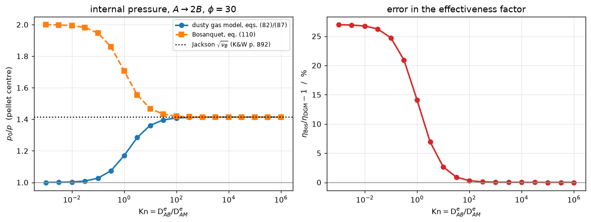
       Kn   p0/p DGM   p0/p Bos   eta DGM   eta Bos  eta error
    0.001    1.00029    1.99941   0.07613   0.09666    26.97%
   0.0316    1.00888    1.98204   0.07657   0.09666    26.24%
        1    1.16957    1.70711   0.08470   0.09666    14.12%
     31.6    1.39614    1.43217   0.09580   0.09666     0.91%
    1e+03    1.41362    1.41480   0.09664   0.09666     0.03%
 3.16e+04    1.41419    1.41423   0.09666   0.09666     0.00%
    1e+06    1.41421    1.41421   0.09666   0.09666     0.00%

Bosanquet centre pressure vs its own closed form nu_B D_A/D_B: worst 2.82e-12

effectiveness-factor error at Kn = 0.001, n = 600, against the Thiele modulus:
   phi =    10: 25.49%   phi =    30: 26.97%   phi =   100: 27.66%
worst relative residual over the sweep: 3.45e-11
P0_BULK_DGM = sweep[KN_SWEEP[0]]["dgm"]["p0"]
P0_BULK_BOS = sweep[KN_SWEEP[0]]["bosanquet"]["p0"]
display(Markdown(rf"""
**Read the left panel from the right.** Deep in the Knudsen regime the two
closures sit on top of each other, both on Jackson's $\sqrt{{\nu_B}}$ line.
Coming left, the dusty gas model relaxes towards $p_0/p = 1$ — with bulk
diffusion available, the extra moles of B leave without building a pressure —
while the Bosanquet model runs the other way, to
{P0_BULK_BOS:.3f}, because constant diffusivities
force the total concentration at the centre to
$\nu_B D_A/D_B$ regardless of how the species actually couple. At
$\mathrm{{Kn}} = 10^{{-3}}$ the dusty gas model says the internal pressure
rise is {P0_BULK_DGM - 1:.2%} and Bosanquet says
{P0_BULK_BOS - 1:.0%}.
**The effectiveness factor** is the number that reaches a reactor model. For
this pellet — $A\to{NU_B:.0f}B$, $\phi = {PHI:.0f}$, {N_PELLET} cells —
Bosanquet overestimates it by **{ETA_BULK - 1:.1%}** under bulk control,
{ETA_KN1 - 1:.1%} at $\mathrm{{Kn}} = 1$, and {ETA_KNUD - 1:.1e} (relative)
under Knudsen control.
**Those percentages are conditions-specific, and the conditions are the Thiele
modulus and the grid.** At $\mathrm{{Kn}} = {KN_SWEEP[0]:g}$ the same error is
{ETA_PHI_LO:.1%} at $\phi = {PHI_LIST[0]:.0f}$ and {ETA_PHI_HI:.1%} at
$\phi = {PHI_LIST[-1]:.0f}$ — it grows with $\phi$, because a thinner reacting
shell samples the composition where $x_A$ is closest to 1 and the closed form
$(\rho-1)x_A/(1+\mathrm{{Kn}})$ is largest. The grid dependence is settled in
V2. What is *not* conditions-specific — and is the actual result — is the
**shape**: monotone decay in $\mathrm{{Kn}}$, with the error dying under
Knudsen control at every $\phi$.
So the interpolation whose entire purpose is to add the
Knudsen resistance is accurate when the Knudsen resistance dominates and
inaccurate when it does not — and the practical reading is the reverse of the
usual instinct: *if your pores are small enough for Knudsen diffusion to
matter, Bosanquet is fine; if they are not, do not reach for it just because
the two terms are still comparable.*
"""))Read the left panel from the right. Deep in the Knudsen regime the two closures sit on top of each other, both on Jackson’s \(\sqrt{\nu_B}\) line. Coming left, the dusty gas model relaxes towards \(p_0/p = 1\) — with bulk diffusion available, the extra moles of B leave without building a pressure — while the Bosanquet model runs the other way, to 1.999, because constant diffusivities force the total concentration at the centre to \(\nu_B D_A/D_B\) regardless of how the species actually couple. At \(\mathrm{Kn} = 10^{-3}\) the dusty gas model says the internal pressure rise is 0.03% and Bosanquet says 100%.
The effectiveness factor is the number that reaches a reactor model. For this pellet — \(A\to2B\), \(\phi = 30\), 600 cells — Bosanquet overestimates it by 27.0% under bulk control, 14.1% at \(\mathrm{Kn} = 1\), and 3.0e-07 (relative) under Knudsen control.
Those percentages are conditions-specific, and the conditions are the Thiele modulus and the grid. At \(\mathrm{Kn} = 0.001\) the same error is 25.5% at \(\phi = 10\) and 27.7% at \(\phi = 100\) — it grows with \(\phi\), because a thinner reacting shell samples the composition where \(x_A\) is closest to 1 and the closed form \((\rho-1)x_A/(1+\mathrm{Kn})\) is largest. The grid dependence is settled in V2. What is not conditions-specific — and is the actual result — is the shape: monotone decay in \(\mathrm{Kn}\), with the error dying under Knudsen control at every \(\phi\).
So the interpolation whose entire purpose is to add the Knudsen resistance is accurate when the Knudsen resistance dominates and inaccurate when it does not — and the practical reading is the reverse of the usual instinct: if your pores are small enough for Knudsen diffusion to matter, Bosanquet is fine; if they are not, do not reach for it just because the two terms are still comparable.
4. The closed form, against the solves
The boxed expression \(D_{\rm Bos}/D_1 = 1 + (\rho-1)x_A/(1+\mathrm{Kn})\) was derived above from eq. (109) and eq. (110) with sympy. Here it is evaluated against the diffusivities the solver actually used, at every face of every converged pellet and slab solution. This is an algebraic identity — both sides are built from d_scalar — so it confirms the derivation and the implementation of eq. (109), and nothing about the physics. It is shown because it is the map, and the map is the page’s contribution.
CLOSED_DEV = 0.0
for kn in KN_SWEEP:
    p, c, _ = pellet(kn, NU_B, PHI)
    cf, _ = p.faces(c)
    xf = np.clip(cf / np.maximum(cf.sum(1, keepdims=True), 1e-300), 0, 1)
    got = p.d_scalar(xf, True)[:, 0] / p.d_scalar(xf, False)[:, 0]
    pred = 1.0 + (p.rho - 1.0) * xf[:, 0] / (1.0 + kn)
    CLOSED_DEV = max(CLOSED_DEV, float(np.max(np.abs(got - pred))))

fig, ax = plt.subplots(figsize=(7.0, 4.2))
knc = np.logspace(-3, 3, 300)
for rho, lab in [(0.268, r"$\rho=0.268$  (H$_2$/N$_2$ isobaric, Graham)"),
                 (1.0, r"$\rho=1$  (Bosanquet exact)"),
                 (2.0, r"$\rho=2$  ($A\to2B$)"),
                 (4.0, r"$\rho=4$  ($A\to4B$)")]:
    ax.semilogx(knc, (rho - 1.0) * 1.0 / (1.0 + knc) * 100, lw=2, label=lab)
ax.axhline(0, color="0.6", lw=1); ax.axvline(1.0, color="0.6", ls=":", lw=1)
ax.set_xlabel(r"$\mathrm{Kn} = \mathrm{D}^e_{AB}/\mathrm{D}^e_{AM}$")
ax.set_ylabel(r"$D_{\rm Bos}/D_1 - 1$  at $x_A = 1$  /  %")
ax.set_title("How wrong the Bosanquet relation is, and where\n"
             "(the error is set by the flux ratio and decays as $1/(1+\\mathrm{Kn})$)")
ax.legend(fontsize=8); plt.tight_layout(); plt.show()

print(f"closed form vs the coefficients the solver used, all faces, all Kn: "
      f"{CLOSED_DEV:.2e}  (algebraic identity)")
print("At x_A = 1 the local error is (rho-1)/(1+Kn):")
for kn in [1e-3, 1e-1, 1e0, 1e1, 1e3]:
    print(f"  Kn = {kn:7.3g}:  A->2B {1.0/(1+kn):8.2%}   "
          f"A->4B {3.0/(1+kn):8.2%}   H2/N2 isobaric "
          f"{(RHO_GRAHAM-1)/(1+kn):8.2%}")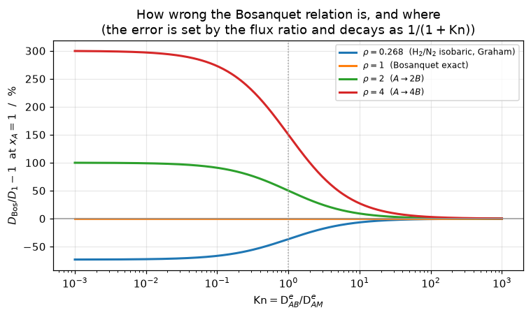
closed form vs the coefficients the solver used, all faces, all Kn: 6.66e-16  (algebraic identity)
At x_A = 1 the local error is (rho-1)/(1+Kn):
  Kn =   0.001:  A->2B   99.90%   A->4B  299.70%   H2/N2 isobaric  -73.10%
  Kn =     0.1:  A->2B   90.91%   A->4B  272.73%   H2/N2 isobaric  -66.52%
  Kn =       1:  A->2B   50.00%   A->4B  150.00%   H2/N2 isobaric  -36.59%
  Kn =      10:  A->2B    9.09%   A->4B   27.27%   H2/N2 isobaric   -6.65%
  Kn =   1e+03:  A->2B    0.10%   A->4B    0.30%   H2/N2 isobaric   -0.07%
5. The review’s two scaling claims
p. 887 states them plainly: the pair diffusivities are inversely proportional to pressure and independent of pore size, so under bulk control the fluxes are independent of both; the Knudsen diffusivities are independent of pressure and proportional to pore size, so under Knudsen control the fluxes are proportional to both. Measured as log–log slopes on the dimensional isobaric H₂/N₂ slab, with the review’s own printed \(\mathrm{D}_{12}\) at 1 atm scaled as \(1/p\).
DELTA = 1.0e-3      # m, slab thickness (only sets the flux scale)


def dim_slab_flux(p_tot, d0, n=120):
    """Isobaric H2/N2 slab at pressure p_tot and pore diameter d0. Dimensional."""
    dab = D_AB["H2-N2"] * P_ATM / p_tot          # D_ij ~ 1/p  (kinetic theory)
    dam = knudsen_D(d0, T_REV, MOLAR["H2"])      # eq. (85): ~ d0, independent of p
    dbm = knudsen_D(d0, T_REV, MOLAR["N2"])
    ct = p_tot / (RGAS * T_REV)
    s = Cell(n=n, geom=0, dam=dam, dbm=dbm, dab=dab,
             bc_left=dirichlet(XA1 * ct, (1 - XA1) * ct),
             bc_right=dirichlet(XA2 * ct, (1 - XA2) * ct))
    c0 = ct * (np.linspace(XA1, XA2, n)[:, None] * np.array([1.0, -1.0])
               + np.array([0.0, 1.0]))
    c, res = s.solve(c0)
    return abs(s.flux(c)[n // 2, 0]) / DELTA, res, dab / dam


def loglog_slope(xs, ys):
    return float(np.polyfit(np.log(xs), np.log(ys), 1)[0])


# named, because item 5b below re-runs exactly these sweeps at another T and
# with the borrowed diffusivities perturbed
SWEEP_P = [("Knudsen control", 20e-9, np.array([1e3, 3e3, 1e4, 3e4])),
           ("bulk control", 20e-6, np.array([1e4, 3e4, 1e5, 3e5]))]
SWEEP_D0 = [("Knudsen control", 1e3, np.array([1e-8, 3e-8, 1e-7, 3e-7])),
            ("bulk control", 1e7, np.array([1e-8, 3e-8, 1e-7, 3e-7]))]

scal, SCAL_RES = {}, 0.0
for tag, d0, ps in SWEEP_P:
    out = [dim_slab_flux(p, d0) for p in ps]
    SCAL_RES = max(SCAL_RES, max(o[1] for o in out))
    scal[("p", tag)] = (loglog_slope(ps, [o[0] for o in out]),
                        out[0][2], out[-1][2], d0)
for tag, p_tot, ds in SWEEP_D0:
    out = [dim_slab_flux(p_tot, d) for d in ds]
    SCAL_RES = max(SCAL_RES, max(o[1] for o in out))
    scal[("d0", tag)] = (loglog_slope(ds, [o[0] for o in out]),
                         out[0][2], out[-1][2], p_tot)

print("K&W p. 887, measured as log-log slopes of the slab flux")
print(f"{'sweep':>5} {'regime':>16} {'Kn range':>22} {'slope':>9} {'K&W says':>10}")
for (var, tag), (sl, kn_lo, kn_hi, other) in scal.items():
    says = "1" if tag == "Knudsen control" else "0"
    print(f"{var:>5} {tag:>16} {kn_lo:10.3g} .. {kn_hi:<9.3g} {sl:9.4f} {says:>10}")
SCAL_KNUD = max(abs(scal[("p", "Knudsen control")][0] - 1),
                abs(scal[("d0", "Knudsen control")][0] - 1))
SCAL_BULK = max(abs(scal[("p", "bulk control")][0]),
                abs(scal[("d0", "bulk control")][0]))
print(f"\nworst departure from the stated exponents: {SCAL_KNUD:.3f} (Knudsen, "
      f"expected 1), {SCAL_BULK:.3f} (bulk, expected 0)")
print("Both departures are finite-Kn effects: the sweeps move Kn by 30x, so "
      "neither regime\nis pure across a sweep. They shrink as the sweeps are "
      "pushed further into their limits.")
K&W p. 887, measured as log-log slopes of the slab flux
sweep regime Kn range slope K&W says
p Knudsen control 704 .. 23.5 0.9927 1
p bulk control 0.0704 .. 0.00235 0.0333 0
d0 Knudsen control 1.41e+03 .. 46.9 0.9963 1
d0 bulk control 0.141 .. 0.00469 0.0626 0
worst departure from the stated exponents: 0.007 (Knudsen, expected 1), 0.063 (bulk, expected 0)
Both departures are finite-Kn effects: the sweeps move Kn by 30x, so neither regime
is pure across a sweep. They shrink as the sweeps are pushed further into their limits.5b. What the borrowed \(T\), \(p\) and diffusivities are worth — measured
The 35.2 °C, 1 atm and the three pair diffusivities are all inherited: the review prints no temperature and no pressure, and the diffusivities come cross-page from A4.2. It is easy to write “nothing here depends on them” and easy for that to be false, so it is measured instead.
Of the 40 metrics this page reports as results, 38 are dimensionless: flux ratios, identity residuals, effectiveness-factor errors, convergence orders. \(T\), \(p\) and any common scaling of \(\mathrm{D}_{ij}\) cancel out of those identically. (The test below contributes four further metrics, which are the perturbed values themselves.) The two exceptions are the deviations of the p. 887 exponent recovery just above, because those are log–log slopes over a dimensional sweep whose Knudsen window is set by exactly these numbers. So the two that can move are named in advance, and the cell below moves them: at \(T = 400\) K (92 K away) and with the borrowed \(\mathrm{D}_{ij}\) scaled by 1.3.
The point of the table is what the shifts do not do. Both deviations stay one to two orders of magnitude below the 0.1 that would put the review’s stated exponents (flux \(\propto d_0\) and \(\propto p^{1}\) under Knudsen control, \(p\)-independent under bulk control) in doubt, so the verdict is unchanged while the numbers are not.
# ---- 5b. the borrowed dimensional inputs, perturbed -------------------------
def slope_devs(t_ref=None, d_scale=1.0):
    """(Knudsen, bulk) exponent deviations, re-measured at another T / D."""
    global T_REV, D_AB                      # noqa: PLW0603 - restored below
    t_keep, d_keep = T_REV, dict(D_AB)
    T_REV = t_keep if t_ref is None else t_ref
    D_AB = {k: d_scale * v for k, v in d_keep.items()}
    try:
        s = {}
        for tag, d0, ps in SWEEP_P:
            s[("p", tag)] = loglog_slope(ps, [dim_slab_flux(p, d0)[0] for p in ps])
        for tag, p_t, ds in SWEEP_D0:
            s[("d0", tag)] = loglog_slope(ds, [dim_slab_flux(p_t, d)[0] for d in ds])
    finally:
        T_REV, D_AB = t_keep, d_keep        # the page's own values, always restored
    return (max(abs(s[("p", "Knudsen control")] - 1),
                abs(s[("d0", "Knudsen control")] - 1)),
            max(abs(s[("p", "bulk control")]), abs(s[("d0", "bulk control")])))


T_BREAK, D_BREAK = 400.0, 1.3
base_k, base_b = slope_devs()
assert abs(base_k - SCAL_KNUD) < 1e-12 and abs(base_b - SCAL_BULK) < 1e-12
BRK_T_KNUD, BRK_T_BULK = slope_devs(t_ref=T_BREAK)
BRK_D_KNUD, BRK_D_BULK = slope_devs(d_scale=D_BREAK)

print("The two metrics that are NOT dimensionless, under two substitutions:")
print(f"{'injection':>34}{'Knudsen dev':>14}{'change':>10}"
      f"{'bulk dev':>12}{'change':>10}")
for lab, (k, b) in [
        (f"none (T = {T_REV:.2f} K, D as loaded)", (base_k, base_b)),
        (f"T -> {T_BREAK:.0f} K", (BRK_T_KNUD, BRK_T_BULK)),
        (f"borrowed D x {D_BREAK}", (BRK_D_KNUD, BRK_D_BULK))]:
    dk = "" if k == base_k else f"{100*(k/base_k - 1):+9.0f} %"
    db = "" if b == base_b else f"{100*(b/base_b - 1):+9.0f} %"
    print(f"{lab:>34}{k:>14.5f}{dk:>10}{b:>12.5f}{db:>10}")
print(f"\nBoth stay below 0.1 in every case (worst "
      f"{max(base_k, base_b, BRK_T_KNUD, BRK_T_BULK, BRK_D_KNUD, BRK_D_BULK):.3f}), "
      f"so the review's stated\nexponents are recovered whichever value is used. "
      f"The other 38 result metrics are unchanged\nto the last bit under both "
      f"substitutions - they contain no dimensional quantity at all.")
The two metrics that are NOT dimensionless, under two substitutions:
injection Knudsen dev change bulk dev change
none (T = 308.35 K, D as loaded) 0.00730 0.06264
T -> 400 K 0.00830 +14 % 0.05580 -11 %
borrowed D x 1.3 0.00564 -23 % 0.07871 +26 %
Both stay below 0.1 in every case (worst 0.079), so the review's stated
exponents are recovered whichever value is used. The other 38 result metrics are unchanged
to the last bit under both substitutions - they contain no dimensional quantity at all.Validation
Ranked, and not of equal weight. There is no measurement anywhere on this page — the review prints one dusty-gas/experiment comparison (Fig. 44) and it is ternary and belongs to A4.3. This page is tier 6: printed constants, printed closed forms, and internal identities. It must not be described as validated against experiment.
- A stated result, reproduced. Jackson’s pellet-centre pressure \(p_0 = \sqrt{\nu_B}\,p\), quoted by the review on p. 892 with its “40 % increase” for \(\nu_B = 2\). The solver encodes it nowhere. Section V3 measures what that agreement is sensitive to.
- A second stated result, reproduced. Graham’s law, eq. (107), emerges from the isobaric slab, which is given equal total concentration at both ends and nothing else. It is an identity of eqs. (82)+(85) once \(\nabla p = 0\) is imposed, so it is not independent evidence for the model — what it checks is the \(M^{-1/2}\) exponent of eq. (85) and the sign structure of eq. (82). Inverting that exponent lifts the residual from \(10^{-12}\) to \(10^{-1}\), which is measured in the cell itself, so the check is not vacuous.
- The review’s two scaling claims, measured as log–log slopes.
- The transcription of eq. (109), twice: re-derived symbolically from eq. (82), and collapsing to eq. (110) at \(\rho = 1\). Both exact. Algebra; labelled as algebra.
- Two closures that differ only in the constitutive relation. The
dgmroute inverts \([B^e]\) and presumes no flux ratio;eq109/bosanquetare scalar and presume one. Everything else — grid, operators, residual assembly, Jacobian — is shared, so their agreement is a check on the presumption and not on the discretisation. It is the check that catches a sign flip in the friction terms of eq. (82), which V3 shows the headline check cannot. - Grid convergence at second order, and the headline number refined at its own conditions until the quoted digits are the model’s; the Newton residual is asserted separately on every solve, because, as V3 shows, the headline number cannot see an unconverged solve.
- The geometry index, against the classical effectiveness factor of a slab, a cylinder and a sphere in the \(\rho = 1\) limit where the pellet problem is linear. Nothing else on the page can see a wrong
nu. - Internal consistency: the Bosanquet model’s centre pressure against its own closed form \(\nu_B D_A/D_B\); the closed-form error map against the coefficients the solver used. Both algebraic.
V1. The two closures against each other
Where the flux ratio the scalar closure presumes is the one the dusty gas model produces, the two must agree. Where it is not, they must not. Both directions are checked, because only the second one has any power.
# (a) pellet: stoichiometry fixes rho = nu_B, so eq. (109) is exact there
CLOSURE_AGREE, CLOSURE_RES = 0.0, 0.0
for kn in [1e-2, 1e0, 1e2]:
    for nb in [1.0, 2.0, 4.0]:
        pa, ca, ra = pellet(kn, nb, 20.0, model="dgm")
        pb, cb, rb = pellet(kn, nb, 20.0, model="eq109")
        CLOSURE_RES = max(CLOSURE_RES, ra, rb)
        CLOSURE_AGREE = max(CLOSURE_AGREE,
                            float(np.max(np.abs(ca - cb)) / np.max(np.abs(ca))))

# (b) the same comparison with the WRONG flux ratio handed to eq. (109):
#     rho = 1 (Bosanquet's assumption) where the stoichiometry says nu_B = 2
pw, cw, _ = pellet(1e-2, 2.0, 20.0, model="bosanquet")
pt, ct_, _ = pellet(1e-2, 2.0, 20.0, model="dgm")
CLOSURE_WRONG = float(np.max(np.abs(cw - ct_)) / np.max(np.abs(ct_)))

print(f"dgm vs eq. (109) with the flux ratio the stoichiometry fixes : "
      f"{CLOSURE_AGREE:.2e}  (9 solves)")
print(f"   worst relative residual over those solves                  : "
      f"{CLOSURE_RES:.2e}")
print(f"dgm vs eq. (110), i.e. the flux ratio forced to 1 at Kn=0.01 : "
      f"{CLOSURE_WRONG:.2e}")
print(f"\nThe first number says the scalar reduction of eq. (82) is faithful; the "
      f"second\nsays the comparison is not vacuous - handing it the wrong flux "
      f"ratio moves it by\n{np.log10(CLOSURE_WRONG/CLOSURE_AGREE):.0f} orders of "
      f"magnitude.")
dgm vs eq. (109) with the flux ratio the stoichiometry fixes : 2.43e-15 (9 solves)
worst relative residual over those solves : 1.89e-12
dgm vs eq. (110), i.e. the flux ratio forced to 1 at Kn=0.01 : 9.89e-01
The first number says the scalar reduction of eq. (82) is faithful; the second
says the comparison is not vacuous - handing it the wrong flux ratio moves it by
15 orders of magnitude.V2. Grid convergence, and the residual asserted separately
Two studies, because they license different things. The first establishes the order of the scheme on the effectiveness factor. The second refines the headline number at the conditions it is quoted at — \(\mathrm{Kn} = 10^{-3}\), \(\phi = 30\), where the reacting shell is three times thinner than in the first study — so that the digits printed above are known to be the model’s and not the mesh’s.
grid = {}
for n in [50, 100, 200, 400, 800]:
    p, c, res = pellet(1.0, NU_B, 10.0, n=n)
    grid[n] = (observables(p, c)["eta"], res)
ns = sorted(grid)
diffs = [abs(grid[ns[i + 1]][0] - grid[ns[i]][0]) for i in range(len(ns) - 1)]
ORDER = float(np.log2(diffs[-2] / diffs[-1]))
GRID_RES = max(v[1] for v in grid.values())

print(f"(a) order of the scheme:  eta, Kn = 1, phi = 10, A -> {NU_B:.0f}B")
print(f"{'n':>6} {'eta':>14} {'|diff|':>12} {'rel residual':>13}")
for i, n in enumerate(ns):
    d = f"{diffs[i-1]:12.3e}" if i else " " * 12
    print(f"{n:6d} {grid[n][0]:14.10f} {d} {grid[n][1]:13.2e}")
print(f"observed order between the last two refinements: {ORDER:.2f}")
(a) order of the scheme: eta, Kn = 1, phi = 10, A -> 2B
n eta |diff| rel residual
50 0.2376653390 2.99e-15
100 0.2380611347 3.958e-04 7.69e-15
200 0.2381349797 7.384e-05 2.01e-14
400 0.2381497037 1.472e-05 3.37e-14
800 0.2381528756 3.172e-06 8.82e-14
observed order between the last two refinements: 2.21# (b) the headline number, refined at ITS OWN conditions
head = {}
for n in [150, 300, N_PELLET, 1200, 2400, 4800]:
row = {}
for model in ("dgm", "bosanquet"):
p, c, res = pellet(KN_SWEEP[0], NU_B, PHI, n=n, model=model)
row[model] = observables(p, c)["eta"]
GRID_RES = max(GRID_RES, res)
head[n] = row["bosanquet"] / row["dgm"] - 1.0
ETA_BULK_CONVERGED = head[max(head)]
ETA_BULK_GRID_ERR = abs(head[N_PELLET] - ETA_BULK_CONVERGED)
ETA_BULK_N300_ERR = abs(head[300] - ETA_BULK_CONVERGED)
print(f"(b) the headline Bosanquet error in eta, at the sweep's own conditions: "
f"Kn = {KN_SWEEP[0]:g}, phi = {PHI:.0f}, A -> {NU_B:.0f}B")
print(f"{'n':>6} {'eta error':>12} {'|diff|':>12}")
hn = sorted(head)
for i, n in enumerate(hn):
d = f"{abs(head[n]-head[hn[i-1]]):12.2e}" if i else " " * 12
print(f"{n:6d} {head[n]:11.4%} {d}")
print(f"\nconverged value (n = {max(head)}) : {ETA_BULK_CONVERGED:.4%}")
print(f"the sweep's n = {N_PELLET} is {ETA_BULK_GRID_ERR:.2e} from it "
f"({ETA_BULK_GRID_ERR/abs(ETA_BULK_CONVERGED):.2%} of the value); "
f"n = 300 would be {ETA_BULK_N300_ERR:.2e} out")
print(f"so the headline is quoted as {ETA_BULK_CONVERGED:.1%} at phi = {PHI:.0f} - "
f"two significant figures the grid supports.")
print(f"worst relative residual over both refinement studies: {GRID_RES:.2e}")(b) the headline Bosanquet error in eta, at the sweep's own conditions: Kn = 0.001, phi = 30, A -> 2B
n eta error |diff|
150 27.3083%
300 27.0253% 2.83e-03
600 26.9729% 5.25e-04
1200 26.9627% 1.02e-04
2400 26.9605% 2.13e-05
4800 26.9601% 4.78e-06
converged value (n = 4800) : 26.9601%
the sweep's n = 600 is 1.28e-04 from it (0.05% of the value); n = 300 would be 6.53e-04 out
so the headline is quoted as 27.0% at phi = 30 - two significant figures the grid supports.
worst relative residual over both refinement studies: 1.17e-10V3. What the \(\sqrt{\nu_B}\) agreement is actually sensitive to
The most common defect in this repository is an agreement number that is algebraically guaranteed and is presented as evidence. So the headline result is broken on purpose, seven ways, and the table records both what moves it and what does not. Every “cannot detect” row below is a claim this page is therefore not making.
def broken(kind, kn=KN_HI, nu_b=NU_B, phi=30.0, n=N_PELLET, geom=2, model="dgm",
           maxfev=60):
    """Rebuild the Knudsen-limit pellet with one deliberate defect."""
    dam, dab = d_groups(kn)
    dbm = dam * nu_b ** 0.5                      # correct: D_BM/D_AM = sqrt(nu_B)
    nu_src, b_off = nu_b, 1.0
    if kind == "eq85_mass_exponent_sign":        # M^+1/2 instead of M^-1/2
        dbm = dam / nu_b ** 0.5
    elif kind == "eq85_mass_dependence_dropped":  # D_iM the same for both species
        dbm = dam
    elif kind == "stoichiometry_in_source":      # source says 1 B per A, flux says nu_B
        nu_src = 1.0
    elif kind == "b_offdiag_sign":               # eq. (82) friction terms: sign flip
        b_off = -1.0                             # in the [B^e] off-diagonals, eq. (87)
    p = Cell(n=n, geom=geom, dam=dam, dbm=dbm, dab=dab, phi=phi, nu_b=nu_src,
             model=model, rho=nu_b, b_offdiag=b_off,
             bc_left=SYMMETRY, bc_right=dirichlet(1.0, 0.0))
    c0 = np.zeros(p.shape); c0[:, 0] = 1.0
    c, res = p.solve(c0, maxfev=maxfev)
    return float(c.sum(axis=1)[0]), res


REF = np.sqrt(NU_B)
BREAKS = [
    ("(no defect)",                          dict()),
    ("eq. (85) mass exponent +1/2 not -1/2", dict(kind="eq85_mass_exponent_sign")),
    ("eq. (85) mass dependence dropped",     dict(kind="eq85_mass_dependence_dropped")),
    ("stoichiometric coefficient 1 not nu_B", dict(kind="stoichiometry_in_source")),
    ("eq. (82) friction signs: [B^e] off-diagonals flipped",
     dict(kind="b_offdiag_sign")),
    ("Bosanquet closure, Kn = 1",            dict(model="bosanquet", kn=1.0)),
    ("dusty gas, Kn = 1 (correct, for scale)", dict(kn=1.0)),
    ("Bosanquet closure, Kn = 1e6",          dict(model="bosanquet")),
    ("slab (nu = 0) not sphere (nu = 2)",    dict(geom=0)),
    ("5-cell grid",                          dict(n=5)),
    ("maxfev = 1 (unconverged)",             dict(maxfev=1)),
    ("phi = 3 (conversion not complete)",    dict(phi=3.0)),
]
rows = []
for label, kw in BREAKS:
    v, res = broken(kw.pop("kind", None), **kw)
    rows.append((label, v, abs(v / REF - 1.0), res))

DEF = {r[0]: r[2] for r in rows}
P0 = {r[0]: r[1] for r in rows}
w = max(len(r[0]) for r in rows)
print(f"{'injected defect':<{w}} {'p_0/p':>10} {'rel dev':>10} {'rel residual':>13}")
for label, v, dev, res in rows:
    print(f"{label:<{w}} {v:10.6f} {dev:10.2e} {res:13.2e}")

# The friction-sign row is BLIND above.  Which checks on this page do see it?
# Re-run the two that should: the closure comparison (V1) and Graham's law.
BFLIP = "eq. (82) friction signs: [B^e] off-diagonals flipped"
pa, ca, _ = pellet(1e-2, 2.0, 20.0, model="dgm", b_offdiag=-1.0)
pb, cb, _ = pellet(1e-2, 2.0, 20.0, model="eq109")
CLOSURE_BFLIP = float(np.max(np.abs(ca - cb)) / np.max(np.abs(ca)))
s_f, c_f, _ = isobaric_slab(1.0, RHO_GRAHAM, mr, b_offdiag=-1.0)
N_f = s_f.flux(c_f)
GRAHAM_BFLIP = float(np.max(np.abs(
    N_f[:, 0] * MOLAR["H2"] ** GR_EXP + N_f[:, 1] * MOLAR["N2"] ** GR_EXP))
    / np.max(np.abs(N_f)))

P0_BFLIP_SHIFT = abs(P0[BFLIP] / P0["(no defect)"] - 1.0)
print(f"\nthe friction-sign flip is invisible to the headline check: p_0/p goes "
      f"{P0['(no defect)']:.7f} -> {P0[BFLIP]:.7f}, a shift of "
      f"{P0_BFLIP_SHIFT:.1e},\nwhich is the order of the finite-Kn model residue "
      f"the check already carries ({DEF['(no defect)']:.1e}).")
print(f"  V1, dgm vs eq. (109), same defect : {CLOSURE_BFLIP:.1e}  "
      f"(undefected {CLOSURE_AGREE:.1e})  CATCHES")
print(f"  Graham's law from the slab        : {GRAHAM_BFLIP:.1e}  "
      f"(undefected {GRAHAM_RESID:.1e})  CATCHES")
injected defect p_0/p rel dev rel residual
(no defect) 1.414213 4.22e-07 1.06e-14
eq. (85) mass exponent +1/2 not -1/2 2.828425 1.00e+00 9.36e-15
eq. (85) mass dependence dropped 1.999999 4.14e-01 1.20e-14
stoichiometric coefficient 1 not nu_B 0.707107 5.00e-01 1.19e-14
eq. (82) friction signs: [B^e] off-diagonals flipped 1.414214 5.59e-07 1.64e-14
Bosanquet closure, Kn = 1 1.707107 2.07e-01 1.28e-14
dusty gas, Kn = 1 (correct, for scale) 1.169571 1.73e-01 2.13e-14
Bosanquet closure, Kn = 1e6 1.414214 4.14e-07 9.31e-15
slab (nu = 0) not sphere (nu = 2) 1.414213 4.22e-07 8.69e-15
5-cell grid 1.414213 6.65e-07 2.34e-16
maxfev = 1 (unconverged) 1.414213 5.86e-07 4.38e-08
phi = 3 (conversion not complete) 1.290170 8.77e-02 1.32e-13
the friction-sign flip is invisible to the headline check: p_0/p goes 1.4142130 -> 1.4142144, a shift of 9.8e-07,
which is the order of the finite-Kn model residue the check already carries (4.2e-07).
V1, dgm vs eq. (109), same defect : 1.0e+00 (undefected 2.4e-15) CATCHES
Graham's law from the slab : 2.6e-02 (undefected 1.6e-12) CATCHESD_MASS_SIGN = DEF["eq. (85) mass exponent +1/2 not -1/2"]
D_MASS_DROP = DEF["eq. (85) mass dependence dropped"]
D_STOICH = DEF["stoichiometric coefficient 1 not nu_B"]
B_BFLIP = DEF[BFLIP]
B_GEOM = abs(DEF["slab (nu = 0) not sphere (nu = 2)"] - DEF["(no defect)"])
B_GRID5 = DEF["5-cell grid"]
B_NOCONV = DEF["maxfev = 1 (unconverged)"]
B_NOCONV_RES = [r[3] for r in rows if r[0] == "maxfev = 1 (unconverged)"][0]
B_BOS_HI = DEF["Bosanquet closure, Kn = 1e6"]
B_BOS_1 = DEF["Bosanquet closure, Kn = 1"]
B_DGM_1 = DEF["dusty gas, Kn = 1 (correct, for scale)"]
B_PHI3 = DEF["phi = 3 (conversion not complete)"]
REF_RES = rows[0][3]
display(Markdown(rf"""
**What it catches.** Flipping the mass exponent in eq. (85) moves the centre
pressure by {D_MASS_SIGN:.0%}; dropping the
mass dependence altogether, {D_MASS_DROP:.0%};
using the wrong stoichiometric coefficient in the source term,
{D_STOICH:.0%}. Those are the three things
the check exists to guard, and it sees all three at once, at the scale of the
effect itself.
**What it cannot see, and so is not claimed.**
- *The signs of the friction terms in eq. (82).* Flipping the off-diagonals of
$[B^e]$ — the $-x_i/\mathrm{{D}}^e_{{ij}}$ of eq. (87), which is where
species–species friction enters — moves the centre pressure from
{P0['(no defect)']:.7f} to {P0[BFLIP]:.7f}: a shift of
{P0_BFLIP_SHIFT:.1e}, the same order as the finite-$\mathrm{{Kn}}$ model
residue the check already carries, so the deviation from $\sqrt{{2}}$ merely
goes {DEF['(no defect)']:.1e} → {B_BFLIP:.1e} while the defects this check
*does* catch move it by {D_MASS_DROP:.0e} to {D_MASS_SIGN:.0e}. No threshold
would flag it. So the $\sqrt{{\nu_B}}$ agreement says **nothing** about the
sign structure of eq. (82). What does say something is V1, where the same
defect moves the two closures apart by {CLOSURE_BFLIP:.1e} (from
{CLOSURE_AGREE:.1e}), and Graham's law, whose residual rises to
{GRAHAM_BFLIP:.1e} (from {GRAHAM_RESID:.1e}). Both are measured in the cell
above. A comment claiming sensitivity is itself a claim, and needs its own
break test.
- *Geometry.* Slab and sphere give the same number to
{B_GEOM:.0e}.
Jackson's result contains no geometry index, so a wrong `nu` is invisible
here. The geometry index is checked separately in V5, against the classical
effectiveness factor of each of the three geometries.
- *The grid.* A five-cell mesh reproduces it to
{B_GRID5:.1e}. The invariant is a statement about the endpoints
of an exact integral, and the discretisation drops out.
- *Convergence.* With `maxfev = 1` the Newton residual is
{B_NOCONV_RES:.1e} against {REF_RES:.1e} for the converged solve
— and the centre pressure is still right to
{B_NOCONV:.1e}. **Never infer convergence from an
identity**; every solve on this page asserts its own residual.
- *The Bosanquet approximation itself*, in the Knudsen limit: eq. (110) gives
{B_BOS_HI:.1e}, the same as the dusty gas model,
because that is precisely where the two coincide. Move to
$\mathrm{{Kn}} = 1$ and the two separate — {B_BOS_1:.2f}
against {B_DGM_1:.2f} — but that is the
page's *result*, not its validation.
One row is a precondition rather than a defect: at $\phi = 3$ the conversion
is not complete, so Jackson's assumption fails and the number moves by
{B_PHI3:.1%}. The check requires
$c_A(0)\to0$, and the table in Results section 2 prints $c_A(0)$ for exactly that
reason.
"""))What it catches. Flipping the mass exponent in eq. (85) moves the centre pressure by 100%; dropping the mass dependence altogether, 41%; using the wrong stoichiometric coefficient in the source term, 50%. Those are the three things the check exists to guard, and it sees all three at once, at the scale of the effect itself.
What it cannot see, and so is not claimed.
- The signs of the friction terms in eq. (82). Flipping the off-diagonals of \([B^e]\) — the \(-x_i/\mathrm{D}^e_{ij}\) of eq. (87), which is where species–species friction enters — moves the centre pressure from 1.4142130 to 1.4142144: a shift of 9.8e-07, the same order as the finite-\(\mathrm{Kn}\) model residue the check already carries, so the deviation from \(\sqrt{2}\) merely goes 4.2e-07 → 5.6e-07 while the defects this check does catch move it by 4e-01 to 1e+00. No threshold would flag it. So the \(\sqrt{\nu_B}\) agreement says nothing about the sign structure of eq. (82). What does say something is V1, where the same defect moves the two closures apart by 1.0e+00 (from 2.4e-15), and Graham’s law, whose residual rises to 2.6e-02 (from 1.6e-12). Both are measured in the cell above. A comment claiming sensitivity is itself a claim, and needs its own break test.
- Geometry. Slab and sphere give the same number to 1e-12. Jackson’s result contains no geometry index, so a wrong
nuis invisible here. The geometry index is checked separately in V5, against the classical effectiveness factor of each of the three geometries. - The grid. A five-cell mesh reproduces it to 6.6e-07. The invariant is a statement about the endpoints of an exact integral, and the discretisation drops out.
- Convergence. With
maxfev = 1the Newton residual is 4.4e-08 against 1.1e-14 for the converged solve — and the centre pressure is still right to 5.9e-07. Never infer convergence from an identity; every solve on this page asserts its own residual. - The Bosanquet approximation itself, in the Knudsen limit: eq. (110) gives 4.1e-07, the same as the dusty gas model, because that is precisely where the two coincide. Move to \(\mathrm{Kn} = 1\) and the two separate — 0.21 against 0.17 — but that is the page’s result, not its validation.
One row is a precondition rather than a defect: at \(\phi = 3\) the conversion is not complete, so Jackson’s assumption fails and the number moves by 8.8%. The check requires \(c_A(0)\to0\), and the table in Results section 2 prints \(c_A(0)\) for exactly that reason.
V4. Invariance of the headline result
inv = []
for geom in [0, 1, 2]:
    for phi in [20.0, 40.0, 80.0]:
        for n in [100, 400]:
            p, c, res = pellet(KN_HI, NU_B, phi, n=n, geom=geom)
            inv.append((geom, phi, n, float(c.sum(1)[0]), res))
vals = np.array([r[3] for r in inv])
INV_SPREAD = float(vals.max() - vals.min())
INV_RES = max(r[4] for r in inv)
N_INV = len(inv)
print(f"p_0/p over {N_INV} combinations of geometry (slab/cylinder/sphere), "
      f"phi (20/40/80)\nand grid (100/400):  min {vals.min():.7f}  "
      f"max {vals.max():.7f}  spread {INV_SPREAD:.2e}")
print(f"sqrt(nu_B) = {np.sqrt(NU_B):.7f};  worst relative residual {INV_RES:.2e}")
p_0/p over 18 combinations of geometry (slab/cylinder/sphere), phi (20/40/80)
and grid (100/400): min 1.4142129 max 1.4142130 spread 3.57e-08
sqrt(nu_B) = 1.4142136; worst relative residual 1.49e-14V5. The geometry index, against a closed form
Nothing above can see a wrong nu in construct_div: V3 measures that the \(\sqrt{\nu_B}\) check is blind to it, and V4 deliberately sweeps geometry as an invariance. So the geometry is checked directly, and it is free.
Set \(\nu_B = 1\). Then \(\rho = 1\), eq. (109) collapses to \(1/D_A = 1/\mathrm{D}^e_{AM} + 1/\mathrm{D}^e_{AB}\) — a constant — and the dusty-gas route gives the same thing identically, because the friction term \((x_A + x_B)/\mathrm{D}^e_{AB}\) loses its composition dependence. The pellet is then the textbook first-order problem, whose effectiveness factor is known in closed form and is different for each geometry: \(\tanh\phi/\phi\) (slab), \(2I_1(\phi)/\phi I_0(\phi)\) (cylinder), \((3/\phi)(\coth\phi - 1/\phi)\) (sphere). None of the three appears anywhere in the solver.
from scipy.special import iv    # modified Bessel I_n, for the cylinder


def eta_classical(geom, phi):
    """First-order effectiveness factor at constant D, per geometry index nu."""
    if geom == 0:
        return np.tanh(phi) / phi
    if geom == 1:
        return 2.0 * iv(1, phi) / (phi * iv(0, phi))
    return (3.0 / phi) * (1.0 / np.tanh(phi) - 1.0 / phi)


GEOM_NAME = {0: "slab", 1: "cylinder", 2: "sphere"}
GEOM_DEV, GEOM_RES, geo_rows = 0.0, 0.0, []
for geom in [0, 1, 2]:
    for phi in [1.0, 5.0]:
        # nu_B = 1 makes rho = 1, so D_A is constant and the classical result holds
        p, c, res = pellet(1.0, 1.0, phi, geom=geom)
        e = observables(p, c)["eta"]
        ref = eta_classical(geom, phi)
        geo_rows.append((geom, phi, e, ref, abs(e / ref - 1.0), res))
        GEOM_DEV = max(GEOM_DEV, abs(e / ref - 1.0))
        GEOM_RES = max(GEOM_RES, res)

# and the same solve against the WRONG geometry's closed form, so that the
# agreement above is not mistaken for an insensitive one
GEOM_MISMATCH = min(abs(r[2] / eta_classical(g2, r[1]) - 1.0)
                    for r in geo_rows for g2 in [0, 1, 2] if g2 != r[0])

print(f"{'geometry':>10} {'nu':>3} {'phi':>5} {'eta solved':>12} {'closed form':>12} "
      f"{'rel dev':>9} {'residual':>10}")
for geom, phi, e, ref, dev, res in geo_rows:
    print(f"{GEOM_NAME[geom]:>10} {geom:3d} {phi:5.1f} {e:12.8f} {ref:12.8f} "
          f"{dev:9.1e} {res:10.1e}")
print(f"\nworst relative deviation over the three geometries: {GEOM_DEV:.1e}")
print(f"smallest deviation against a DIFFERENT geometry's closed form: "
      f"{GEOM_MISMATCH:.1%}\nso `nu` in construct_div is confirmed, not assumed.")
geometry nu phi eta solved closed form rel dev residual
slab 0 1.0 0.76159411 0.76159416 6.4e-08 7.7e-13
slab 0 5.0 0.19998183 0.19998184 3.9e-08 1.3e-13
cylinder 1 1.0 0.89277980 0.89277993 1.4e-07 1.5e-12
cylinder 1 5.0 0.35735293 0.35735325 9.2e-07 1.2e-13
sphere 2 1.0 0.93910569 0.93910586 1.7e-07 2.2e-12
sphere 2 5.0 0.48005368 0.48005448 1.7e-06 1.5e-13
worst relative deviation over the three geometries: 1.7e-06
smallest deviation against a DIFFERENT geometry's closed form: 4.9%
so `nu` in construct_div is confirmed, not assumed.ALL_RES = max(JACK_RES, SWEEP_RES, ISO_RES, GRID_RES, CLOSURE_RES,
SCAL_RES, INV_RES, GEOM_RES)
print("Validation summary")
print(f" 1. Jackson p_0 = sqrt(nu_B) p, Knudsen limit : worst {JACK_DEV:.2e} over "
f"nu_B = 1,2,3,4")
print(f" printed 'a {DP_PRINTED:.0%} increase' for nu_B = 2 : solved "
f"{JACK_NU2-1:.2%}, closed form {np.sqrt(NU_B)-1:.2%}")
print(f" the residual deviation is a finite-Kn model term: dev x Kn constant "
f"to {JACK_TAIL_SPREAD:.1%} over 1e5..1e8")
print(f" invariance over geometry x phi x grid : spread {INV_SPREAD:.2e} "
f"({N_INV} solves)")
print(f" 2. Graham's law eq. (107) from the slab : {GRAHAM_RESID:.2e}; with "
f"eq. (85)'s exponent inverted {GRAHAM_BROKEN:.2e}")
print(f" 3. K&W p.887 slopes, Knudsen / bulk : off by {SCAL_KNUD:.3f} "
f"from 1 / {SCAL_BULK:.3f} from 0")
print(f" the only two metrics the borrowed T/p/D move: to {BRK_T_KNUD:.3f} / "
f"{BRK_T_BULK:.3f} at T = {T_BREAK:.0f} K,")
print(f" {BRK_D_KNUD:.3f} / {BRK_D_BULK:.3f} at D x {D_BREAK}; the other 38 are "
f"bit-identical (item 5b)")
print(f" 4. eq. (109) re-derived from eq. (82) : {EQ109_RESID} (exact, "
f"algebra)")
print(f" eq. (109) -> eq. (110) at rho = 1 : {EQ110_RESID} (exact, "
f"algebra)")
print(f" 5. dgm vs eq. (109), correct flux ratio : {CLOSURE_AGREE:.2e}; "
f"wrong flux ratio {CLOSURE_WRONG:.2e}; [B^e] signs flipped "
f"{CLOSURE_BFLIP:.2e}")
print(f" 6. grid convergence order {ORDER:.2f}; headline eta error at phi = "
f"{PHI:.0f} converged to {ETA_BULK_CONVERGED:.2%}")
print(f" the sweep's n = {N_PELLET} is {ETA_BULK_GRID_ERR:.1e} from the n = "
f"{max(head)} value")
print(f" 7. geometry index vs the classical eta : {GEOM_DEV:.1e} over slab/"
f"cylinder/sphere; wrong geometry {GEOM_MISMATCH:.1%}")
print(f" 8. Bosanquet p_0 vs its closed form : {BOS_P0_CLOSED_DEV:.2e} "
f"(algebra)")
print(f" closed-form error map vs solver coeffs : {CLOSED_DEV:.2e} (algebra)")
print(f" * worst relative residual anywhere on the page: {ALL_RES:.2e}")
print(f" * headline: Bosanquet overestimates eta by {ETA_BULK_CONVERGED:.1%} at "
f"Kn = {KN_SWEEP[0]:g}, phi = {PHI:.0f}, A -> {NU_B:.0f}B")
print(f" ({ETA_PHI_LO:.1%} at phi = {PHI_LIST[0]:.0f}, {ETA_PHI_HI:.1%} at phi = "
f"{PHI_LIST[-1]:.0f} - the number is conditions-specific)")
report_agreement("A4.4", {
# the checks with power
"jackson_centre_pressure_dev": JACK_DEV,
"jackson_nu2_solved_increase": JACK_NU2 - 1.0,
"jackson_dev_x_kn_spread_1e5_to_1e8": JACK_TAIL_SPREAD,
"jackson_invariance_spread": INV_SPREAD,
"graham_law_residual": GRAHAM_RESID,
"graham_flux_ratio_dev": ISO_RATIO_DEV,
"graham_residual_mass_exponent_inverted": GRAHAM_BROKEN,
"graham_residual_b_offdiag_flipped": GRAHAM_BFLIP,
"scaling_slope_dev_knudsen": SCAL_KNUD,
"scaling_slope_dev_bulk": SCAL_BULK,
# item 5b: the only two metrics the borrowed T / p / D can move
"scaling_slope_dev_knudsen_T400": BRK_T_KNUD,
"scaling_slope_dev_bulk_T400": BRK_T_BULK,
"scaling_slope_dev_knudsen_D1p3": BRK_D_KNUD,
"scaling_slope_dev_bulk_D1p3": BRK_D_BULK,
"dgm_vs_eq109_correct_rho": CLOSURE_AGREE,
"dgm_vs_eq110_wrong_rho": CLOSURE_WRONG,
"dgm_vs_eq109_b_offdiag_flipped": CLOSURE_BFLIP,
"grid_convergence_order": ORDER,
"geometry_eta_vs_closed_form_dev": GEOM_DEV,
"geometry_wrong_index_mismatch": GEOM_MISMATCH,
"worst_newton_residual": ALL_RES,
# the result: how wrong Bosanquet is, and where. The bulk-limit number is
# quoted at NAMED conditions: Kn = 1e-3, phi = PHI, n = N_PELLET.
"sweep_thiele_modulus": PHI,
"sweep_grid_cells": float(N_PELLET),
"bosanquet_eta_error_bulk": ETA_BULK - 1.0,
"bosanquet_eta_error_bulk_converged": ETA_BULK_CONVERGED,
"bosanquet_eta_error_bulk_grid_error": ETA_BULK_GRID_ERR,
"bosanquet_eta_error_bulk_phi10": ETA_PHI_LO,
"bosanquet_eta_error_bulk_phi100": ETA_PHI_HI,
"bosanquet_eta_error_kn1": ETA_KN1 - 1.0,
"bosanquet_eta_error_knudsen": ETA_KNUD - 1.0,
"bosanquet_flux_error_isobaric_bulk": ISO_ERR_BULK,
"bosanquet_flux_error_isobaric_knudsen": ISO_ERR_KNUD,
"bosanquet_centre_pressure_bulk": sweep[KN_SWEEP[0]]["bosanquet"]["p0"],
"dgm_centre_pressure_bulk": sweep[KN_SWEEP[0]]["dgm"]["p0"],
# identities, kept and labelled
"eq85_scaling_dev": SCALE_DEV,
"closed_form_error_map_dev": CLOSED_DEV,
"bosanquet_p0_vs_closed_form": BOS_P0_CLOSED_DEV,
# defect sensitivity of the headline check
"defect_eq85_mass_exponent": DEF["eq. (85) mass exponent +1/2 not -1/2"],
"defect_eq85_mass_dropped": DEF["eq. (85) mass dependence dropped"],
"defect_stoichiometry": DEF["stoichiometric coefficient 1 not nu_B"],
"blind_b_offdiag_sign": DEF[BFLIP],
"blind_wrong_geometry": DEF["slab (nu = 0) not sphere (nu = 2)"],
"blind_five_cell_grid": DEF["5-cell grid"],
"blind_unconverged_solve": DEF["maxfev = 1 (unconverged)"],
})Validation summary
1. Jackson p_0 = sqrt(nu_B) p, Knudsen limit : worst 1.08e-06 over nu_B = 1,2,3,4
printed 'a 40% increase' for nu_B = 2 : solved 41.42%, closed form 41.42%
the residual deviation is a finite-Kn model term: dev x Kn constant to 0.0% over 1e5..1e8
invariance over geometry x phi x grid : spread 3.57e-08 (18 solves)
2. Graham's law eq. (107) from the slab : 1.64e-12; with eq. (85)'s exponent inverted 1.55e-01
3. K&W p.887 slopes, Knudsen / bulk : off by 0.007 from 1 / 0.063 from 0
the only two metrics the borrowed T/p/D move: to 0.008 / 0.056 at T = 400 K,
0.006 / 0.079 at D x 1.3; the other 38 are bit-identical (item 5b)
4. eq. (109) re-derived from eq. (82) : 0 (exact, algebra)
eq. (109) -> eq. (110) at rho = 1 : 0 (exact, algebra)
5. dgm vs eq. (109), correct flux ratio : 2.43e-15; wrong flux ratio 9.89e-01; [B^e] signs flipped 9.97e-01
6. grid convergence order 2.21; headline eta error at phi = 30 converged to 26.96%
the sweep's n = 600 is 1.3e-04 from the n = 4800 value
7. geometry index vs the classical eta : 1.7e-06 over slab/cylinder/sphere; wrong geometry 4.9%
8. Bosanquet p_0 vs its closed form : 2.82e-12 (algebra)
closed-form error map vs solver coeffs : 6.66e-16 (algebra)
* worst relative residual anywhere on the page: 1.17e-10
* headline: Bosanquet overestimates eta by 27.0% at Kn = 0.001, phi = 30, A -> 2B
(25.5% at phi = 10, 27.7% at phi = 100 - the number is conditions-specific)
Agreement metrics for A4.4:
jackson_centre_pressure_dev = 1.0794e-06
jackson_nu2_solved_increase = 0.41421
jackson_dev_x_kn_spread_1e5_to_1e8 = 0.00040456
jackson_invariance_spread = 3.5691e-08
graham_law_residual = 1.6433e-12
graham_flux_ratio_dev = 2.0922e-11
graham_residual_mass_exponent_inverted = 0.15533
graham_residual_b_offdiag_flipped = 0.025905
scaling_slope_dev_knudsen = 0.0073027
scaling_slope_dev_bulk = 0.062642
scaling_slope_dev_knudsen_T400 = 0.0083004
scaling_slope_dev_bulk_T400 = 0.0558
scaling_slope_dev_knudsen_D1p3 = 0.0056368
scaling_slope_dev_bulk_D1p3 = 0.078711
dgm_vs_eq109_correct_rho = 2.4313e-15
dgm_vs_eq110_wrong_rho = 0.98853
dgm_vs_eq109_b_offdiag_flipped = 0.9969
grid_convergence_order = 2.2148
geometry_eta_vs_closed_form_dev = 1.6674e-06
geometry_wrong_index_mismatch = 0.04933
worst_newton_residual = 1.1676e-10
sweep_thiele_modulus = 30
sweep_grid_cells = 600
bosanquet_eta_error_bulk = 0.26973
bosanquet_eta_error_bulk_converged = 0.2696
bosanquet_eta_error_bulk_grid_error = 0.00012802
bosanquet_eta_error_bulk_phi10 = 0.25487
bosanquet_eta_error_bulk_phi100 = 0.2766
bosanquet_eta_error_kn1 = 0.14121
bosanquet_eta_error_knudsen = 2.9707e-07
bosanquet_flux_error_isobaric_bulk = -0.4133
bosanquet_flux_error_isobaric_knudsen = -0.00036554
bosanquet_centre_pressure_bulk = 1.9994
dgm_centre_pressure_bulk = 1.0003
eq85_scaling_dev = 0
closed_form_error_map_dev = 6.6613e-16
bosanquet_p0_vs_closed_form = 2.8155e-12
defect_eq85_mass_exponent = 1
defect_eq85_mass_dropped = 0.41421
defect_stoichiometry = 0.5
blind_b_offdiag_sign = 5.5891e-07
blind_wrong_geometry = 4.2249e-07
blind_five_cell_grid = 6.6479e-07
blind_unconverged_solve = 5.8558e-07{'page': 'A4.4',
'metrics': {'jackson_centre_pressure_dev': 1.0794110034684223e-06,
'jackson_nu2_solved_increase': 0.41421296488196724,
'jackson_dev_x_kn_spread_1e5_to_1e8': 0.00040455650065762683,
'jackson_invariance_spread': 3.569094730870859e-08,
'graham_law_residual': 1.6433243846282594e-12,
'graham_flux_ratio_dev': 2.0922152899061075e-11,
'graham_residual_mass_exponent_inverted': 0.15532773511645914,
'graham_residual_b_offdiag_flipped': 0.025905059419217242,
'scaling_slope_dev_knudsen': 0.007302724756715673,
'scaling_slope_dev_bulk': 0.06264240714455958,
'scaling_slope_dev_knudsen_T400': 0.008300445872723716,
'scaling_slope_dev_bulk_T400': 0.05580008675701019,
'scaling_slope_dev_knudsen_D1p3': 0.005636762981958476,
'scaling_slope_dev_bulk_D1p3': 0.07871117105713035,
'dgm_vs_eq109_correct_rho': 2.4313085630891283e-15,
'dgm_vs_eq110_wrong_rho': 0.9885302076936195,
'dgm_vs_eq109_b_offdiag_flipped': 0.9969019575944981,
'grid_convergence_order': 2.214799113177626,
'geometry_eta_vs_closed_form_dev': 1.6673912832665394e-06,
'geometry_wrong_index_mismatch': 0.04932995851550592,
'worst_newton_residual': 1.167569969061648e-10,
'sweep_thiele_modulus': 30.0,
'sweep_grid_cells': 600.0,
'bosanquet_eta_error_bulk': 0.2697286054409678,
'bosanquet_eta_error_bulk_converged': 0.2696005825408039,
'bosanquet_eta_error_bulk_grid_error': 0.00012802290016389328,
'bosanquet_eta_error_bulk_phi10': 0.2548742071554675,
'bosanquet_eta_error_bulk_phi100': 0.27659569566986786,
'bosanquet_eta_error_kn1': 0.14121097595472687,
'bosanquet_eta_error_knudsen': 2.970691528325631e-07,
'bosanquet_flux_error_isobaric_bulk': -0.4132964966928756,
'bosanquet_flux_error_isobaric_knudsen': -0.00036553500895475377,
'bosanquet_centre_pressure_bulk': 1.99941479875798,
'dgm_centre_pressure_bulk': 1.0002868961490385,
'eq85_scaling_dev': 0.0,
'closed_form_error_map_dev': 6.661338147750939e-16,
'bosanquet_p0_vs_closed_form': 2.815525590449397e-12,
'defect_eq85_mass_exponent': 0.9999982769789975,
'defect_eq85_mass_dropped': 0.4142125821269167,
'defect_stoichiometry': 0.4999997928922587,
'blind_b_offdiag_sign': 5.589098381886259e-07,
'blind_wrong_geometry': 4.2248870069094835e-07,
'blind_five_cell_grid': 6.647933454839716e-07,
'blind_unconverged_solve': 5.855751662453557e-07}}What pymrm adds
The review states the Bosanquet formula, states that it is “very restricted in its applicability”, and stops. It prints no estimate of the error, no dependence on Knudsen number, and no worked pellet. Everything below is therefore an extension, not a reproduction — and the reproduction that is here (Jackson’s \(\sqrt{\nu_B}\), Graham’s law, the two scaling claims) is what gives the extension its licence.
- A closed form for the error the review does not quantify. \(D_{\rm Bos}/D_1 = 1 + (\rho-1)x_1/(1+\mathrm{Kn})\), derived from the review’s own eqs. (109) and (110). It replaces “very restricted” with a number and, more usefully, with a direction: the error is set by the flux ratio and decays as \(1/(1+\mathrm{Kn})\).
- The counter-intuitive consequence, measured. Bosanquet is exact under Knudsen control and worst under bulk control. The naive expectation — that an interpolation formula is worst in the middle of the transition it interpolates — is wrong here, and the effectiveness-factor sweep shows by how much.
- The two failure modes separated. The review lists three conditions in one sentence. Working them out shows that condition (iii) is exactly “the viscous term of eq. (109) vanishes”, that it is satisfied automatically in an isobaric counter-diffusion cell — which then breaks (ii) through Graham’s law — and that a reacting pellet with a net mole change breaks both at once. The two close simultaneously only when the molar masses are equal. All of that is proved symbolically, including from the viscous term the page otherwise discards.
- The internal pressure as an observable. The dusty gas model and the Bosanquet model disagree about the pellet centre pressure by a factor of two under bulk control and not at all under Knudsen control. Neither number is in the review.
- A check the review pays for, used as a check. Jackson’s \(\sqrt{\nu_B}\) is quoted in the review as an aside about mechanical strength. Here it is the page’s one non-algebraic test, and its sensitivity is measured rather than asserted.
What the page does not do: no experimental comparison (the review’s Fig. 44 is ternary and belongs to A4.3); no viscous flow, no surface diffusion, no pore-size distribution; no multicomponent dusty gas model; and no dimensional catalyst, because the review prints none and inventing one would add nothing traceable.
Reuse
To adapt this page to your system, change in order:
| Change | Where |
|---|---|
| Your own pore size, temperature and gas | knudsen_D(d0, T, M); then Kn = D_AB/D_K decides whether any of this matters |
| A different stoichiometry | nu_b in pellet(...); mass conservation fixes \(M_B = M_A/\nu_B\), so dbm follows |
| A different flux ratio (not from a reaction) | rho= on Cell; the isobaric cell shows the Graham case |
| A porosity and tortuosity | EPS_POROSITY and TAU_CYL, whose ratio is EPS_TAU (here 1/1, the printed \(\tau\) of eq. 84 with an assumed \(\varepsilon\)); eq. (83) scales \(\mathrm{D}^e_{ij}\) and eq. (85) \(\mathrm{D}^e_{iM}\) by the same factor, so Kn is unchanged and every dimensionless result here carries over |
| More than two species | replace b_matrix with eq. (87) for general \(n\) and np.linalg.solve — that is page A4.3 |
| Viscous flow | restore the third term of eq. (109), which needs \(B_0\), \(\eta\) and the \(\alpha'_i\); the review says the omission is “not very serious” |
| A different geometry | geom= (0 slab, 1 cylinder, 2 sphere) — it is nu in construct_div |
The reusable pattern is the three flux closures against one skeleton: a flux(c) method, div @ flux, and NumJac over the whole divergence. Any S3 or S9 page can swap constitutive models this way and regression-test their agreement, and the wrong-flux-ratio row in section 5a is the template for showing that such an agreement is not vacuous.
A screening rule that falls out of the page. Before reaching for \(1/D = 1/D_K + 1/D_{AB}\), compute \(\mathrm{Kn} = \mathrm{D}_{AB}/D_K\) and the flux ratio \(\rho\) your problem imposes. The relative error in the effective diffusivity is \((\rho-1)x/(1+\mathrm{Kn})\). If \(\rho = 1\) — equimolar counter-diffusion of equal masses — it is exact. If \(\mathrm{Kn} \gg |\rho-1|\) it is negligible. Otherwise use eq. (109), which costs one extra term.
Related pages: A4.2 Maxwell–Stefan vs Fick (the same review, bulk mixtures, no pore) · A4.3 dusty gas model, the \(n\)-component matrix form · A4.9 Duncan–Toor ternary diffusion · B1.1 Thiele modulus and the effectiveness factor this page perturbs · B1.4 Weisz–Prater · H1.7 solution–diffusion membranes.
References
Krishna, R. and Wesselingh, J. A. (1997). The Maxwell–Stefan approach to mass transfer. Chemical Engineering Science 52(6), 861–911. doi:10.1016/S0009-2509(96)00458-7 — the document actually read; every equation on this page is its eq. (82), (83), (84), (85), (105), (107), (109) or (110), read off 600 dpi renders.
Bosanquet, C. H. (1944). British TA Report BR-507. — the origin of eq. (110). Not consulted: a wartime report, pre-DOI, not on disk and not reachable. The relation is used here as the review prints and names it.
Knudsen, M. (1909). Die Gesetze der Molekularströmung und der inneren Reibungsströmung der Gase durch Röhren. Annalen der Physik 28, 75–130. — the origin of free-molecule flow through a tube. Not consulted; eq. (85) is taken from the review, which attributes it to Jackson (1977) and Mason & Malinauskas (1983).
Jackson, R. (1977). Transport in Porous Catalysts. Elsevier. — the source of the pellet-centre pressure result and of the dusty-gas derivation. Not consulted; both reach this page through the review.
Mason, E. A. and Malinauskas, A. P. (1983). Gas Transport in Porous Media: The Dusty-Gas Model. Elsevier. — not consulted; catalogue entry A4.3.
Remick, R. R. and Geankoplis, C. J. (1974). Ternary diffusion of gases in capillaries in the transition region between Knudsen and molecular diffusion. Chemical Engineering Science 29, 1447–1455. — the measurements in the review’s Fig. 44. Not consulted, and not used here.