# Bootstrap: the pymrm this page was checked with, and the gallery files it was
# published with. Works in a checkout, in CI and on a fresh Colab VM.
GALLERY_REF = "gallery-2026.11.10.3"  # replaced by the release tag at publication
PYMRM = ">=3.3.0,<4"  # equals meta.yaml pymrm_min_version, up to the next major
PAGE = "A3.15-graetz-nusselt"  # equals the page directory

import os, sys, urllib.request
from pathlib import Path
_shared = next((p / "shared" for p in (Path.cwd(), *Path.cwd().parents)
                if (p / "shared" / "gallery_bootstrap.py").is_file()), None)
if _shared is None:
    _shared = (Path(os.environ.get("XDG_CACHE_HOME") or Path.home() / ".cache")
               / "pymrm-gallery" / GALLERY_REF)
    _shared.mkdir(parents=True, exist_ok=True)
    urllib.request.urlretrieve(
        "https://raw.githubusercontent.com/computational-chemical-engineering/"
        f"pymrm-gallery/{GALLERY_REF}/shared/gallery_bootstrap.py",
        _shared / "gallery_bootstrap.py")
sys.path.insert(0, str(_shared))
sys.modules.pop("gallery_bootstrap", None)
from gallery_bootstrap import setup
setup(PAGE, PYMRM, GALLERY_REF); # the semicolon stops the cell echoing the pathThe Graetz–Nusselt problem: the constants Graetz could not compute
sec:A
struct:S6
tier:T0
data:tier1
phase:liquid
The developing thermal boundary layer in a tube, solved as a 2-D PDE, and the two amplitudes Graetz declared out of reach and calibrated out of his own apparatus instead.
The Graetz–Nusselt problem: the constants Graetz could not compute
Catalog ID: A3.15 · Structure: S6 (2-D PDE) · Tier: T0
Leo Graetz did not set out to found a branch of convective heat transfer. He was trying to measure the thermal conductivity of liquids, and the problem now named after him is the calculation he needed in order to read his own instrument.
The calculation stopped one step short. He obtained the eigenvalues, and then wrote that the amplitudes multiplying them would need “an exhaustive investigation of the function \(V(r,\beta,R)\), which is probably not simple”, so for physical purposes he determined them experimentally, as constants of the apparatus.
This page computes them, and then asks what that does to his measurements. The answer is not the one the framing suggests.
import time
import warnings
from math import gamma

import numpy as np
import pandas as pd
import matplotlib.pyplot as plt
from scipy.interpolate import CubicSpline
from scipy.optimize import brentq, fsolve
from scipy.special import jn_zeros
from gallery_utils import load_data, load_meta, cite_data, Claims
from model import (GraetzTube, decay, V_profile, eigen, amplitudes,  # this page's model.py
                   series_coeffs, theta_series, invert)

plt.rcParams.update({"figure.dpi": 110, "axes.grid": True, "grid.alpha": 0.3})
claims = Claims(PAGE.split("-")[0])
BREAK = []


def brk(row, metric, broken):
    """One injected defect: ``broken`` is what claim ``metric`` becomes with it."""
    caught = claims.breaks(row, metric, broken)
    BREAK.append((row, metric, claims[metric], float(broken), caught))
    return caught


_SOLVES = {}


def solve2d(**kw):
    """The 2-D Newton solve for the given GraetzTube arguments, computed once."""
    key = tuple(sorted(kw.items(), key=lambda kv: kv[0]))
    if key not in _SOLVES:
        tube = GraetzTube(**kw)
        _SOLVES[key] = (tube, tube.solve())
    return _SOLVES[key]
Background
Everything quoted from the paper below is in the original German with a translation. Nothing load-bearing rests on a translation alone.
Graetz’s apparatus (his §2) is a flow calorimeter. Liquid at temperature \(T_1\) flows under a constant head through a narrow brass tube whose wall is held at the temperature \(T_0\) of running cooling water; the outflow temperature \(U\) and the weight \(G\) collected in one minute are measured. From \(T_0\), \(T_1\), \(U\), \(G\) and the tube length \(l\) the conductivity follows, if you can solve for the temperature field inside the tube.
That is the Graetz problem. He solves it twice.
First with a flat velocity profile (§3), which gives Bessel functions and the classical \(J_0\) zeros. He then says plainly that this will not do:
“Die Annahme jedoch, dass die Flüssigkeit in jedem Punkte der Röhre dieselbe mittlere Geschwindigkeit \(\alpha\) habe, ist weder in der Natur erfüllt, noch wie die Berechnung zeigt, zur Vereinfachung erlaubt.”
(The assumption that the liquid has the same mean velocity \(\alpha\) at every point of the tube is neither fulfilled in nature nor, as the calculation shows, permissible even as a simplification.)
Then with the Poiseuille profile, which is the problem that carries his name. The radial equation is no longer Bessel’s, and the eigenfunctions are, as he notes, an extension of the Bessel functions that he expects “may perhaps possess independent mathematical interest”.
Two things make this worth a page rather than a footnote:
- It is the ancestor of every entrance-length correlation in heat and mass transfer, and the asymptotic Nusselt number of a tube at constant wall temperature is the first eigenvalue of this problem squared and halved.
- The paper contains measurements (six liquids, three pressure heads), and it contains a calibration step whose weakness is invisible from inside the paper and obvious from outside it.
The published model
The equation (journal page 87, read from the page image):
\[ 2\alpha\left(1 - \frac{r^{2}}{R^{2}}\right)\frac{\partial u}{\partial z} = a^{2}\left(\frac{\partial^{2}u}{\partial r^{2}} + \frac{1}{r}\frac{\partial u}{\partial r}\right), \qquad a^{2} = \frac{k}{\varrho C}, \]
with \(u\) measured from the wall temperature, \(u = T_1\) at \(z = 0\) and \(u = 0\) at \(r = R\). \(\alpha\) is the mean velocity, so \(2\alpha(1-r^2/R^2)\) is Poiseuille flow. Axial conduction is present in his plug-flow equation on page 83 and dropped here; §7 of the validation checks that.
The separation \(u = A\,e^{-(a^{2}/2\alpha)\beta^{2}z}V\) gives
\[ \frac{\mathrm{d}^{2}V}{\mathrm{d}r^{2}} + \frac{1}{r}\frac{\mathrm{d}V}{\mathrm{d}r} + \beta^{2}\left(1 - \frac{r^{2}}{R^{2}}\right)V = 0, \qquad V(r,\beta,\infty) = J_{0}(\beta r), \]
and the eigenvalues are the roots \(\mu = \beta R\) of \(V(R,\beta,R) = 0\). Graetz expands \(V\) in powers of \(x = \beta r\) and prints the resulting polynomial in \(\mu\) and its first two roots.
The measurable (page 88) is the mean outlet temperature
\[ U = T_{1}\sum_{i} p_{i}\, \exp\!\left(-\frac{a^{2}\mu_{i}^{2}\pi l \varrho}{2G}\right), \]
and since \(a^{2} = k/(\varrho C)\) the density cancels, so the observations give \(k/c\) directly, which is what his tables report. The tube radius cancels too, a point he makes explicitly on page 82.
And then the step this page is about (page 88):
“Darin sind die \(p_i\) Constanten, die ausser von den \(\mu_i\) nur von \(R\) abhängen. Es wäre natürlich von wesentlichem Vortheil, wenn sich die \(p_i\) bestimmt durch \(R\) und \(\mu_i\) ausdrücken liessen. Indess gehört dazu eine eingehende Untersuchung der Function \(V(r,\beta,R)\), die wahrscheinlich nicht einfach ist, die aber als Erweiterung der Bessel’schen Function vielleicht selbstständiges mathematisches Interesse besitzt. Für physikalische Zwecke lassen sich dagegen die \(p_i\) sehr einfach als Constanten des Apparates experimentell bestimmen.”
(Therein the \(p_i\) are constants which, besides on the \(\mu_i\), depend only on \(R\). It would of course be of essential advantage if the \(p_i\) could be expressed definitely through \(R\) and \(\mu_i\). However, that requires an exhaustive investigation of the function \(V(r,\beta,R)\), which is probably not simple, but which as an extension of the Bessel function may perhaps possess independent mathematical interest. For physical purposes, on the other hand, the \(p_i\) can very simply be determined experimentally as constants of the apparatus.)
He then keeps two terms, and fits \(p_1\), \(p_2\) and \(k/c\) to three runs of one liquid at three pressure heads. Three constants, three observations.
Parameters and assumptions
His: steady state; fully developed Poiseuille flow from \(z = 0\); constant wall temperature; constant \(k\), \(\varrho\), \(c\) over the run; no axial conduction in the Poiseuille case; the measured outflow temperature equals the cross-section mean of \(u\) at \(z = l\); and, for the working formula, two terms of the series suffice, “Das zweite Glied macht noch etwa 3 Proc. in dem Werthe von \(k\) aus” (the second term still accounts for about 3 per cent in the value of \(k\)).
Ours: the same, written in dimensionless form. With \(s = r/R\) and
\[ x \;=\; \frac{a^{2}z}{2\alpha R^{2}} \;=\; \frac{a^{2}\pi z}{2\dot V} \;=\; \frac{(k/c)\,\pi z}{2G}, \]
the whole problem loses every parameter:
\[ (1-s^{2})\frac{\partial\theta}{\partial x} = \frac{1}{s}\frac{\partial}{\partial s}\!\left(s\frac{\partial\theta}{\partial s}\right) + \frac{1}{\mathrm{Pe}^{2}}\frac{\partial^{2}\theta}{\partial x^{2}}, \qquad \theta(0,s) = 1,\quad \theta(x,1) = 0, \]
with \(\theta = (T-T_0)/(T_1-T_0)\) and \(\mathrm{Pe} = 2\alpha R/a^{2}\) the axial Péclet number. Setting \(1/\mathrm{Pe}^{2} = 0\) is Graetz’s equation exactly. \(x\) is twice the Graetz coordinate \(x^{*} = z/(D_{h}\mathrm{Re}\,\mathrm{Pr})\) used in the modern literature.
The cup-mean (flow-weighted) outlet temperature is what a collected sample measures:
\[ \theta_{\text{cup}}(x) = 4\!\int_{0}^{1}(1-s^{2})\,\theta\,s\,\mathrm{d}s = \sum_{i} p_{i}\,e^{-\mu_{i}^{2}x}. \]
Note that Graetz’s own page-88 formula integrates \(V\) against \(r\,\mathrm{d}r\) and divides by \(R^{2}\pi\): that is the area mean, not the cup mean. §8f measures what the difference is worth.
The data
Two files. graetz-1882-observations.csv is all the runs of his §4: six liquids, the three temperatures, the collected weight, and the \(k/c\) and \(k\) he computes from them. graetz-1882-printed-constants.csv is every constant printed in §§2–4 with the journal page it is on, including the series coefficients and the two fitted amplitudes.
These are measurements, which makes this one of the few tier-1 pages in the gallery, but the \(k/c\) column is derived, by his two-term formula with his two fitted amplitudes. The raw measurement is the four temperature-and-mass columns, and this page inverts those independently.
Read the sidecars before using either file. They record: three rows flagged because the fit that uses them has zero degrees of freedom; the internal consistency checks (T = (T₁+U)/2, k = c·(k/c)) and the one liquid that fails the second; and three printed defects in the constants file. No other page’s dataset is loaded.
obs = load_data("graetz-1882-observations.csv", page=PAGE)
con = load_data("graetz-1882-printed-constants.csv", page=PAGE)
obs_meta = load_meta("graetz-1882-observations.csv", page=PAGE)
con_meta = load_meta("graetz-1882-printed-constants.csv", page=PAGE)
C = dict(zip(con.quantity, con.value))
# journal page each constant is printed on, as an integer, so that statements
# like "N pages earlier" are computed from the file rather than typed
PAGE_OF = {q: int(str(s).split()[-1]) for q, s in zip(con.quantity, con.source)}

obs["theta"] = (obs.T_out_C - obs.T_bath_C) / (obs.T_in_C - obs.T_bath_C)
CAL = obs[obs.calibration_row == 1].reset_index(drop=True)

print(f"{len(obs)} runs, {obs.liquid.nunique()} liquids, "
      f"{len(con)} printed constants")
print(obs.groupby("liquid", sort=False)
         .agg(runs=("theta", "size"), G_min=("mass_flow_g_min", "min"),
              G_max=("mass_flow_g_min", "max"), theta_min=("theta", "min"),
              theta_max=("theta", "max")).to_string())
print(f"\n{cite_data(obs_meta)}")


def mean_T_check(t_mean):
    """|(T_in + T_out)/2 - printed T| per row, for a given reading of the mean."""
    return (t_mean - obs.T_mean_C_printed).abs()


# the two integrity checks the tables pay for, both stated in the sidecar
print("\nintegrity check 1:  T = (T_in + T_out)/2, which the paper states on p. 90")
dT = mean_T_check(0.5 * (obs.T_in_C + obs.T_out_C))
N_TMEAN_EXACT = claims.count("T_mean_rows_within_0p02", dT.values, 0.02, above=False,
                             min_margin=1e-3, relative=False,
                             note="rows with |(T_in+T_out)/2 - T| below 0.02 K; margin in K")
print(f"   exact in {N_TMEAN_EXACT} of {len(obs)} rows; "
      f"worst residual {dT.max():.2f} K "
      f"({int((obs.calibration_row[dT > 0.02] == 1).sum())} of the "
      "offenders are the calibration rows, which are means of five observations)")
print("\nintegrity check 2:  k = c * (k/c)")
for liq, g in obs.groupby("liquid", sort=False):
    imp = g.k_printed / g.k_over_c_printed
    stated = g.specific_heat.iloc[0]
    flag = ("" if (pd.isna(stated) or abs(imp.mean() / stated - 1) < 0.01)
            else f"   <-- {abs(imp.mean() / stated - 1) * 100:.1f} % gap")
    print(f"   {liq:11s} stated c = {stated!s:>5}   implied {imp.mean():.4f} "
          f"+/- {imp.std():.4f}{flag}")
print("   turpentine is a printed slip in one of the two numbers, not scatter;")
print("   the page works in k/c throughout, so nothing here depends on it.")

# the three flagged rows, up front
print("\nthe three rows Graetz fitted p1, p2 and k/c to (his stars, p. 91):")
print(CAL[["pressure_head", "T_in_C", "T_out_C", "T_bath_C", "mass_flow_g_min",
           "theta", "k_over_c_printed"]].to_string(index=False))
print(f"   flow range {CAL.mass_flow_g_min.max()/CAL.mass_flow_g_min.min():.2f}x, "
      "three constants, three observations -> zero degrees of freedom")
51 runs, 6 liquids, 37 printed constants
runs G_min G_max theta_min theta_max
liquid
water 13 8.6320 36.4430 0.273514 0.682817
cuso4 11 13.8571 46.6320 0.431746 0.745387
alcohol 7 3.1790 17.3435 0.078408 0.580882
nacl 7 25.0960 36.5595 0.590014 0.673511
znso4 8 32.7445 37.2430 0.660529 0.681419
turpentine 5 13.5690 19.5123 0.506574 0.606418
Graetz, L. (1882) — Annalen der Physik 254(1) 79-94 — doi:10.1002/andp.18822540106 — table
integrity check 1: T = (T_in + T_out)/2, which the paper states on p. 90
exact in 44 of 51 rows; worst residual 0.51 K (3 of the offenders are the calibration rows, which are means of five observations)
integrity check 2: k = c * (k/c)
water stated c = nan implied 1.0019 +/- 0.0006
cuso4 stated c = 0.95 implied 0.9494 +/- 0.0007
alcohol stated c = 0.62 implied 0.6197 +/- 0.0005
nacl stated c = 0.96 implied 0.9615 +/- 0.0022
znso4 stated c = 0.94 implied 0.9387 +/- 0.0017
turpentine stated c = 0.45 implied 0.4317 +/- 0.0003 <-- 4.1 % gap
turpentine is a printed slip in one of the two numbers, not scatter;
the page works in k/c throughout, so nothing here depends on it.
the three rows Graetz fitted p1, p2 and k/c to (his stars, p. 91):
pressure_head T_in_C T_out_C T_bath_C mass_flow_g_min theta k_over_c_printed
II 33.37 25.26 7.2 34.9341 0.690103 0.0969
III 37.76 20.87 7.2 13.8571 0.447317 0.0969
I 32.76 26.13 7.2 46.2492 0.740610 0.0969
flow range 3.34x, three constants, three observations -> zero degrees of freedomPyMRM implementation
The 2-D solve produces the first eigenvalue and its amplitude without ever forming an eigenfunction, so it is an independent witness against the series route in §3 of the validation. It lives in GraetzTube in this page’s model.py.
construct_div(..., nu=1)on the radial axis: cylindrical geometry, which is what puts the \(\tfrac{1}{s}\partial_s(s\,\partial_s)\) in the equation. The axial axis isnu=0, Cartesian. The state is laid out(n_z, n_r), the marching axis first.- Every
bccarries its physical equation in a comment, becauseais written on the outward normal and therefore means different things at the two ends of an axis. - First-order upwind is not good enough here. The exact problem has no axial diffusion at all, so upwind numerical diffusion is pure error and it converges at first order (§3 and the break table measure it). The axial convective face values are van Leer TVD. Because the limiter makes the equations nonlinear, the solve is Newton with the exact Jacobian of the limited flux from
ConvFluxTVD,newton(damping="monotone", stagnation=True), from \(\theta = 1\) everywhere. The conduction operators are linear and assembled once in the constructor; each Newton iteration only evaluates the limited flux and factorises. - A second solver route for the same discrete equations,
solve_deferred: one LU of the first-order upwind operator, the limiter correction lagged in the right-hand side and the update relaxed by \(\omega\). The cell below measures what it needs: at \(\omega = 1\) the sweeps settle into a period-two cycle instead of converging, and below 1 they converge to the Newton field. It is the faster route on these grids (the times are printed), so it is the natural check; it is not used for any published number.
PUB = dict(n_z=600, n_r=128)
NEWTON_TOL = 1e-11          # GraetzTube.solve default; theta is of order one
t0 = time.perf_counter()
TUBE, SOL = solve2d(**PUB)
T_NEWTON = time.perf_counter() - t0
t0 = time.perf_counter()
DEF = TUBE.solve_deferred(omega=0.6)
T_DEF = time.perf_counter() - t0
ROUTE_GAP = float(np.max(np.abs(DEF["theta"] - SOL["theta"])))
print(f"published grid n_z = {PUB['n_z']}, n_r = {PUB['n_r']}: "
      f"{TUBE.shape[0] * TUBE.shape[1]} unknowns")
print(f"  Newton, ConvFluxTVD, damping='monotone': {SOL['nit']} iterations "
      f"(here {T_NEWTON:.1f} s)")
print(f"  deferred correction, omega = 0.6:         {DEF['nit']} sweeps "
      f"(here {T_DEF:.1f} s)")
print(f"  largest difference between the two fields below 1e-10 (here {ROUTE_GAP:.1e})")
claims.bound("newton_vs_deferred_field", ROUTE_GAP, max=1e-10, basis="tolerance",
             note="Newton tol 1e-11, sweeps to an unrelaxed change of 1e-11")


def omega_scan(n_z, n_r, omegas, maxit=400):
    """Sweeps to convergence (or the last change) of deferred correction per omega."""
    tube = GraetzTube(n_z=n_z, n_r=n_r)
    ref = tube.solve()["theta"]
    out = []
    for om in omegas:
        d = tube.solve_deferred(omega=om, maxit=maxit, raise_on_stall=False)
        out.append((om, d["nit"], d["incr"], float(np.max(np.abs(d["theta"] - ref)))))
    return out


print("\n  the relaxation, measured on n_z = 300, n_r = 64 (400 sweeps at most):")
print(f"  {'omega':>7}{'sweeps':>8}   converged to the Newton field")
for om, nit, incr, gap in omega_scan(300, 64, (1.0, 0.9, 0.8, 0.7, 0.6, 0.5)):
    print(f"  {om:7.1f}{nit:8d}   "
          + ("yes, below 1e-10" if gap < 1e-10 else
             f"NO: still changing by {incr:.1e} per sweep, {gap:.1e} from it"))


def period_two(tube, omega, sweeps=120):
    """Last change per sweep, and the change over two sweeps, after ``sweeps``."""
    a = tube.solve_deferred(omega=omega, maxit=sweeps, tol=0.0, raise_on_stall=False)
    b = tube.solve_deferred(omega=omega, maxit=sweeps - 2, tol=0.0, raise_on_stall=False)
    return a["incr"], float(np.max(np.abs(a["theta"] - b["theta"]))) / a["incr"]


OM1_INCR, OM1_P2 = period_two(TUBE, 1.0)
print(f"\n  omega = 1 on the published grid, after 120 sweeps: each sweep still changes "
      f"the field by {OM1_INCR:.1e},")
print(f"  while two sweeps return it to within 1e-3 of that change "
      f"(here {OM1_P2:.1e}): a period-two cycle, not a slow convergence.")
claims.value("deferred_omega1_change_after_120", OM1_INCR, rtol=0.05)
claims.bound("deferred_omega1_period2_ratio", OM1_P2, max=1e-3, basis="chosen",
             note="change over two sweeps over the change per sweep; 0 for an exact cycle")
published grid n_z = 600, n_r = 128: 76800 unknowns
Newton, ConvFluxTVD, damping='monotone': 6 iterations (here 2.9 s)
deferred correction, omega = 0.6: 26 sweeps (here 0.6 s)
largest difference between the two fields below 1e-10 (here 3.7e-12)
the relaxation, measured on n_z = 300, n_r = 64 (400 sweeps at most):
omega sweeps converged to the Newton field
1.0 400 NO: still changing by 2.0e-04 per sweep, 9.9e-05 from it
0.9 256 yes, below 1e-10
0.8 59 yes, below 1e-10
0.7 28 yes, below 1e-10
0.6 26 yes, below 1e-10
0.5 34 yes, below 1e-10
omega = 1 on the published grid, after 120 sweeps: each sweep still changes the field by 1.5e-04,
while two sweeps return it to within 1e-3 of that change (here 1.5e-04): a period-two cycle, not a slow convergence.And the series route, which exists so that the 2-D solve has something independent to be checked against. eigen shoots the radial ODE; amplitudes projects the uniform inlet profile onto the eigenfunctions with the weight \((1-s^{2})s\) that makes them orthogonal. No grid and no pymrm operator is involved.
The cup and area amplitudes come out of the same integral with different weights, which is exactly the difference between what Graetz wrote down and what his thermometer measured.
MU = eigen()
P_CUP, P_AREA, IDENT = amplitudes(MU)
SIGMA = jn_zeros(0, 10)          # the plug-flow case, Graetz's p. 83
P_PLUG = 4.0 / SIGMA ** 2        # and his own amplitudes for it, p. 84

print(f"{'i':>2}{'mu_i':>12}{'p_i (cup)':>12}{'p_i (area)':>12}"
      f"{'sigma_i (plug)':>16}{'4/sigma_i^2':>13}")
for i in range(6):
    print(f"{i+1:2d}{MU[i]:12.6f}{P_CUP[i]:12.6f}{P_AREA[i]:12.6f}"
          f"{SIGMA[i]:16.6f}{P_PLUG[i]:13.6f}")
_sl = np.polyfit(np.log(np.arange(1, 11)), np.log(P_CUP), 1)[0]
print(f"\nsum of the first 10: cup {P_CUP.sum():.4f}, area {P_AREA.sum():.4f} "
      f"(both -> 1 as more modes")
print(f"are added, but only as p_i ~ i^{_sl:.2f}, so a truncated series is a real "
      "approximation)")
print(f"identity N_i = -V'(1)/mu_i^2 holds below 1e-6 (here {IDENT.max():.1e}): it "
      "follows from")
print("the ODE itself, so it checks the trapezoidal quadrature, not the physics.")
claims.value("p1_cup", P_CUP[0], rtol=1e-6)
claims.value("p2_cup", P_CUP[1], rtol=1e-6)
claims.value("nu_infinity", MU[0] ** 2 / 2, rtol=1e-6)
claims.bound("amplitude_quadrature_identity", IDENT.max(), max=1e-6, basis="tolerance",
             note="trapezoid on 40001 points; the ODE makes it zero")
i mu_i p_i (cup) p_i (area) sigma_i (plug) 4/sigma_i^2
1 2.704364 0.819050 0.581121 2.404826 0.691660
2 6.679031 0.097527 0.133770 5.520078 0.131271
3 10.673380 0.032504 0.061885 8.653728 0.053414
4 14.671078 0.015440 0.036607 11.791534 0.028769
5 18.669872 0.008788 0.024575 14.930918 0.017943
6 22.669143 0.005584 0.017822 18.071064 0.012249
sum of the first 10: cup 0.9891, area 0.8964 (both -> 1 as more modes
are added, but only as p_i ~ i^-2.67, so a truncated series is a real approximation)
identity N_i = -V'(1)/mu_i^2 holds below 1e-6 (here 3.2e-08): it follows from
the ODE itself, so it checks the trapezoidal quadrature, not the physics.Results
Three views of the same field: the developing profile, the cup-mean decay that is what Graetz measures, and the local Nusselt number that connects the two ends of the tube to their classical limits.
MU1_2D, P1_2D = decay(SOL["x"], SOL["cup"])
x_nu, Nu = TUBE.nusselt(SOL["theta"])
C_LEVEQUE = 2.0 / (gamma(4.0 / 3.0) * 9.0 ** (1.0 / 3.0))

fig, axes = plt.subplots(1, 3, figsize=(13.0, 3.8))

xs_show = [1e-4, 1e-3, 1e-2, 0.05, 0.2]
for xt, col in zip(xs_show, plt.cm.viridis(np.linspace(0.1, 0.85, len(xs_show)))):
    j = np.argmin(abs(SOL["x"] - xt))
    axes[0].plot(np.r_[SOL["theta"][j], 0.0], np.r_[TUBE.s_c, 1.0], color=col,
                 lw=1.7, label=f"$x$ = {SOL['x'][j]:.0e}".replace("e-0", "e-"))
axes[0].set(xlabel=r"$\theta$", ylabel=r"$s = r/R$",
            title="the boundary layer eating inwards")
axes[0].legend(fontsize=7.5, loc="lower left")

one = P_CUP[0] * np.exp(-MU[0] ** 2 * SOL["x"])
ser = np.array([np.sum(P_CUP * np.exp(-MU ** 2 * xx)) for xx in SOL["x"]])
ser2 = np.array([np.sum(P_CUP[:2] * np.exp(-MU[:2] ** 2 * xx)) for xx in SOL["x"]])
axes[1].semilogx(SOL["x"], SOL["cup"] / one, color="tab:blue", lw=2.0, label="2-D solve")
axes[1].semilogx(SOL["x"], ser / one, "r:", lw=1.6, label="10-term series")
axes[1].semilogx(SOL["x"], ser2 / one, "g-.", lw=1.2, label="2 terms")
axes[1].axhline(1.0, color="k", ls="--", lw=1.0)
gm = ((obs.k_over_c_printed * np.pi * obs.tube_length_cm)
      / (2 * obs.mass_flow_g_min)).values
axes[1].axvspan(gm.min(), gm.max(), color="tab:orange", alpha=0.16)
axes[1].text(gm.min() * 1.05, 1.45, "his runs", fontsize=8, color="tab:orange")
axes[1].set(xlabel=r"$x = (k/c)\pi z/2G$", xlim=(3e-4, 1.0), ylim=(0.95, 1.7),
            ylabel=r"$\theta_{\rm cup}\,/\,p_1e^{-\mu_1^2x}$",
            title="how many terms the thermometer needs")
axes[1].legend(fontsize=8)

m = x_nu > 3e-5
axes[2].loglog(x_nu[m], Nu[m], color="tab:blue", lw=2.0, label="2-D solve")
axes[2].loglog(x_nu[m], C_LEVEQUE * (x_nu[m] / 2) ** (-1 / 3), "k--", lw=1.1,
               label=r"Leveque $\propto x^{-1/3}$")
axes[2].axhline(MU[0] ** 2 / 2, color="tab:red", lw=1.2, ls=":")
axes[2].text(2e-2, MU[0] ** 2 / 2 * 1.09, r"$\mu_1^2/2$", color="tab:red", fontsize=9)
axes[2].set(xlabel=r"$x$", ylabel=r"local $\mathrm{Nu}$", ylim=(2, 300),
            title="both ends have a closed form")
axes[2].legend(fontsize=8)
fig.tight_layout()
plt.show()

print(f"2-D solve, n_z = {PUB['n_z']}, n_r = {PUB['n_r']}, {SOL['nit']} Newton iterations")
print(f"  mu_1 from the far-field decay   {MU1_2D:.6f}")
print(f"  p_1  from the far-field decay   {P1_2D:.6f}")
print(f"  asymptotic Nu = mu_1^2/2        {MU1_2D**2/2:.4f}")
print(f"  Graetz's printed mu_1           {C['graetz_root_mu1']}")
print(f"  Graetz's fitted p_1             {C['p1_working_formula']}   <-- the "
      "constant he could not compute")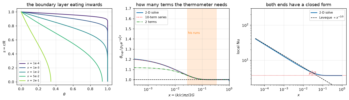
2-D solve, n_z = 600, n_r = 128, 6 Newton iterations
  mu_1 from the far-field decay   2.704379
  p_1  from the far-field decay   0.819396
  asymptotic Nu = mu_1^2/2        3.6568
  Graetz's printed mu_1           2.7043
  Graetz's fitted p_1             0.91264   <-- the constant he could not compute
Validation
Seven checks and a defect-injection table. Two are against constants Graetz prints, two against limits he never had, one is the arithmetic of his own calibration re-run, one is the claim he makes about axial conduction, and one is grid refinement on both axes and in the inlet region separately, followed by §3b, which splits the agreement at the published grid into its two error components.
# 1. His printed power series, against exact rational arithmetic.
#    V = sum a_k x^2k with a_k = sum_j c[k][j] mu^-2j; the recurrence follows from
#    the ODE. Setting x = mu collapses it to a polynomial in mu^2, which is what
#    he prints. Nothing here touches the pymrm solve.
exact_poly = series_coeffs()
printed_poly = [1.0, -C["series_coeff_mu2"], C["series_coeff_mu4"],
                -C["series_coeff_mu6"], C["series_coeff_mu8"],
                -C["series_coeff_mu10"]]


def poly_errors(exact):
    """Relative error of each printed coefficient against ``exact``."""
    return np.array([abs(printed_poly[k] / exact[k] - 1) if exact[k] else 0.0
                     for k in range(6)])


poly_err = poly_errors(exact_poly)
print("1. The polynomial Graetz prints for V(mu) = 0 (journal p. 87)")
print(f"   {'power':>7}{'printed':>18}{'exact (rationals)':>22}{'rel. error':>13}")
for k in range(6):
    flag = "   <-- wrong" if poly_err[k] > 1e-4 else ""
    print(f"   mu^{2*k:<4d}{printed_poly[k]:18.10g}{exact_poly[k]:22.10g}"
          f"{poly_err[k]:13.2e}{flag}")
N_EXACT_COEF = claims.count("series_coeffs_right_to_printed_digits", poly_err[1:], 1e-4,
                            above=False, min_margin=0.5,
                            note="printed coefficients mu^2..mu^10 within 1e-4 relative; "
                                 "relative distance of the nearest to 1e-4")
print(f"   {N_EXACT_COEF} of the 5 printed coefficients are exact to every digit he "
      "prints (the mu^0 term is 1),")
print("   which is a strong check on the page-image reading: the text layer gives 0.1575")
print("   for the 0.1875 above. The last two are arithmetic slips of his: "
      f"{(printed_poly[4] / exact_poly[4] - 1) * 100:+.2f} % and a")
print(f"   factor of {1/(printed_poly[5]/exact_poly[5]):.2f}.")
claims.value("series_coeff_mu8_printed_err", poly_err[4], rtol=1e-3)
claims.value("series_coeff_mu10_printed_err", poly_err[5], rtol=1e-3)

# The one glyph on the page that had to be argued rather than simply read. The
# factor-of-2.65 claim turns on it, so state what the alternative would give.
MU10_ALT = -9.4938e-9            # the same digits with the broken group read as 9
MU10_ALT_ERR = abs(MU10_ALT / exact_poly[5] - 1)
print("\n   ONE CAVEAT ON THE READING, because a headline number turns on it.")
print("   The third digit-group of the mu^10 coefficient is a BROKEN GLYPH on the")
print("   300 dpi bitmap. Magnified 16x it has an open left side, two left-hand")
print("   terminals and no closed upper bowl, so it is a 3 and the coefficient is")
print(f"   {printed_poly[5]:.4e}, which is the factor of "
      f"{1/(printed_poly[5]/exact_poly[5]):.2f} above. Had it been a 9:")
print(f"     read as 3 (taken here) {printed_poly[5]:12.4e}   "
      f"rel err {poly_err[5]:.3f}   <-- factor {1/(printed_poly[5]/exact_poly[5]):.2f}")
print(f"     read as 9 (rejected)   {MU10_ALT:12.4e}   "
      f"rel err {MU10_ALT_ERR:.3f}   <-- {MU10_ALT_ERR*100:.1f} %, an ordinary rounding slip")
print("   So the mu^8 slip stands whatever this glyph is, but the mu^10 FACTOR")
print("   rests on one damaged character read at 16x. The sidecar records it.")
1. The polynomial Graetz prints for V(mu) = 0 (journal p. 87)
power printed exact (rationals) rel. error
mu^0 1 1 0.00e+00
mu^2 -0.1875 -0.1875 0.00e+00
mu^4 0.007921 0.007921006944 8.77e-07
mu^6 -0.00014404 -0.0001440429687 2.06e-05
mu^8 1.4592e-06 1.450798379e-06 5.79e-03 <-- wrong
mu^10 -3.4938e-09 -9.26714482e-09 6.23e-01 <-- wrong
3 of the 5 printed coefficients are exact to every digit he prints (the mu^0 term is 1),
which is a strong check on the page-image reading: the text layer gives 0.1575
for the 0.1875 above. The last two are arithmetic slips of his: +0.58 % and a
factor of 2.65.
ONE CAVEAT ON THE READING, because a headline number turns on it.
The third digit-group of the mu^10 coefficient is a BROKEN GLYPH on the
300 dpi bitmap. Magnified 16x it has an open left side, two left-hand
terminals and no closed upper bowl, so it is a 3 and the coefficient is
-3.4938e-09, which is the factor of 2.65 above. Had it been a 9:
read as 3 (taken here) -3.4938e-09 rel err 0.623 <-- factor 2.65
read as 9 (rejected) -9.4938e-09 rel err 0.024 <-- 2.4 %, an ordinary rounding slip
So the mu^8 slip stands whatever this glyph is, but the mu^10 FACTOR
rests on one damaged character read at 16x. The sidecar records it.# 2. The eigenvalues. His mu_1 is excellent and his mu_2 is not, and the reason
# is visible in his own polynomial.
def positive_roots(poly):
"""Positive real roots mu of a polynomial in mu^2 (coefficients low to high)."""
r = np.sort(np.roots(poly[::-1]))
return np.sqrt(r[(abs(r.imag) < 1e-9) & (r.real > 0)].real)
print("2. Eigenvalues")
roots_printed = positive_roots(printed_poly)
roots_exact_t = positive_roots(exact_poly)
mu1_err = abs(C["graetz_root_mu1"] / MU[0] - 1)
mu2_err = abs(C["graetz_root_mu2"] / MU[1] - 1)
print(f" mu_1 printed {C['graetz_root_mu1']:<9.4f} exact {MU[0]:.6f}"
f" rel {mu1_err:.2e}")
print(f" mu_2 printed {C['graetz_root_mu2']:<9.2f} exact {MU[1]:.6f}"
f" rel {mu2_err:.2e} <-- {mu2_err*100:.1f} % low")
print(f" his own 10th-order polynomial has positive roots at "
f"{np.array2string(roots_printed, precision=4)},")
print(f" and with the coefficients CORRECTED it has "
f"{np.array2string(roots_exact_t, precision=4)}. So the series can place")
print(" mu_1 to four figures and cannot place mu_2 at all: the 6.50 he prints")
print(" comes from neither polynomial, and truncation, not arithmetic, is why.")
claims.value("mu1_printed_rel_err", mu1_err, rtol=0.01)
claims.value("mu2_printed_rel_err", mu2_err, rtol=1e-3)
print("\n plug-flow zeros he prints (p. 83), against J_0:")
BESSEL_KEYS = ["bessel_zero_1", "bessel_zero_2", "bessel_zero_3", "bessel_zero_4"]
def bessel_errs(zeros):
return np.array([abs(C[k] / zeros[i] - 1) for i, k in enumerate(BESSEL_KEYS)])
for i, key in enumerate(BESSEL_KEYS):
print(f" sigma_{i+1} printed {C[key]:<12.6f} exact {SIGMA[i]:.6f}"
f" rel {abs(C[key]/SIGMA[i]-1):.2e}")
claims.value("bessel_zeros_printed_max_err", bessel_errs(SIGMA).max(), rtol=0.01)2. Eigenvalues
mu_1 printed 2.7043 exact 2.704364 rel 2.38e-05
mu_2 printed 6.50 exact 6.679031 rel 2.68e-02 <-- 2.7 % low
his own 10th-order polynomial has positive roots at [ 2.7046 5.9548 17.4641],
and with the coefficients CORRECTED it has [2.7044]. So the series can place
mu_1 to four figures and cannot place mu_2 at all: the 6.50 he prints
comes from neither polynomial, and truncation, not arithmetic, is why.
plug-flow zeros he prints (p. 83), against J_0:
sigma_1 printed 2.404928 exact 2.404826 rel 4.26e-05
sigma_2 printed 5.520240 exact 5.520078 rel 2.93e-05
sigma_3 printed 8.653870 exact 8.653728 rel 1.64e-05
sigma_4 printed 11.791560 exact 11.791534 rel 2.17e-06# 3. The 2-D pymrm solve against the series route, refined on each axis
# separately. These share NO code: one is a finite-volume solve of the PDE,
# the other shoots the radial ODE and projects. They share only the physics.
# Orders come from successive differences of three levels, so the other
# axis's fixed error cancels and the exact value is not needed.
LADDERS = {"n_z": (dict(n_r=256), (75, 150, 300, 600, 1200)),
"n_r": (dict(n_z=800), (16, 32, 64, 128))}
def ladder(tag, **kw):
"""mu_1 and p_1 along one ladder; ``kw`` are extra GraetzTube arguments."""
fixed, sweep = LADDERS[tag]
v = []
for n in sweep:
_, s_ = solve2d(**fixed, **kw, **{tag: n})
v.append(decay(s_["x"], s_["cup"]))
return np.array(sweep), np.array(v)
def orders(vals):
"""Observed orders from successive differences, one per three levels."""
d = np.diff(vals)
return np.log2(d[:-1] / d[1:])
print("3. 2-D solve vs the eigenfunction route, refining one axis at a time")
LAD = {}
for tag in LADDERS:
fixed = LADDERS[tag][0]
ns, v = ladder(tag)
LAD[tag] = v
om, op = orders(v[:, 0]), orders(v[:, 1])
print(f" refine {tag} ({', '.join(f'{k} = {w}' for k, w in fixed.items())}); "
"order from the three levels ending at that row:")
print(f" {tag:>6}{'mu_1':>12}{'err':>11}{'order':>8}"
f"{'p_1':>12}{'err':>11}{'order':>8}")
for i, n in enumerate(ns):
o = ("", "") if i < 2 else (f"{om[i-2]:8.2f}", f"{op[i-2]:8.2f}")
print(f" {n:6d}{v[i, 0]:12.6f}{v[i, 0]/MU[0]-1:+11.2e}{o[0]:>8}"
f"{v[i, 1]:12.6f}{v[i, 1]/P_CUP[0]-1:+11.2e}{o[1]:>8}")
ORD_AX, ORD_RAD = orders(LAD["n_z"][:, 0]), orders(LAD["n_r"][:, 0])
LADDER_FLOOR = {t: np.abs(np.diff(LAD[t][:, 0])).min() / NEWTON_TOL for t in LAD}
print(f" axial orders in mu_1 {np.array2string(ORD_AX, precision=2)}, radial "
f"{np.array2string(ORD_RAD, precision=2)}: both axes second order, the axial")
print(" one approaching 2 from below as the limiter clips less. The smallest")
print(" difference on either ladder is more than 1e3 times the Newton tolerance.")
claims.bound("order_mu1_axial", ORD_AX[-1], min=1.8, max=2.1, basis="theory",
note="successive differences, n_z 300/600/1200 at n_r 256")
claims.bound("order_mu1_axial_min", ORD_AX.min(), min=1.75, max=2.1, basis="theory",
note="all triples from n_z = 75; pre-asymptotic below 2")
claims.bound("order_mu1_radial", ORD_RAD[-1], min=1.9, max=2.1, basis="theory",
note="successive differences, n_r 32/64/128 at n_z 800")
claims.bound("order_mu1_radial_min", ORD_RAD.min(), min=1.9, max=2.1, basis="theory",
note="all triples from n_r = 16")
claims.bound("ladder_axial_finest_diff_over_tol", LADDER_FLOOR["n_z"], min=1e3,
basis="theory", note="smallest successive mu_1 difference over Newton tol")
claims.bound("ladder_radial_finest_diff_over_tol", LADDER_FLOOR["n_r"], min=1e3,
basis="theory", note="smallest successive mu_1 difference over Newton tol")
# What first-order upwind would cost for the same axial error: its ladder is
# linear (one LU solve per rung), order 1, so it needs C/err cells.
_, UPW = ladder("n_z", limiter=None)
ORD_UPW = orders(UPW[:, 0])
print(f"\n first-order upwind on the same ladder: orders "
f"{np.array2string(ORD_UPW, precision=2)} (what it costs is in 3b, on the axial error alone).")3. 2-D solve vs the eigenfunction route, refining one axis at a time
refine n_z (n_r = 256); order from the three levels ending at that row:
n_z mu_1 err order p_1 err order
75 2.712921 +3.16e-03 0.839088 +2.45e-02
150 2.706697 +8.63e-04 0.824528 +6.69e-03
300 2.704943 +2.14e-04 1.83 0.820456 +1.72e-03 1.84
600 2.704487 +4.54e-05 1.95 0.819411 +4.40e-04 1.96
1200 2.704369 +1.57e-06 1.94 0.819138 +1.07e-04 1.94
refine n_r (n_z = 800); order from the three levels ending at that row:
n_r mu_1 err order p_1 err order
16 2.695190 -3.39e-03 0.817902 -1.40e-03
32 2.702148 -8.20e-04 0.818925 -1.53e-04
64 2.703878 -1.80e-04 2.01 0.819175 +1.52e-04 2.03
128 2.704310 -2.00e-05 2.00 0.819237 +2.28e-04 2.01
axial orders in mu_1 [1.83 1.95 1.94], radial [2.01 2. ]: both axes second order, the axial
one approaching 2 from below as the limiter clips less. The smallest
difference on either ladder is more than 1e3 times the Newton tolerance.
first-order upwind on the same ladder: orders [0.9 0.97 0.97] (what it costs is in 3b, on the axial error alone).3b. What the published mu1_rel_err_2d is.
The single agreement number at the published grid is not an accuracy: the axial and radial errors carry opposite signs and largely cancel there. The two ladders above measure each component without using the published grid. The axial ladder runs at \(n_r = 256\), so its Richardson limit in \(n_z\) is the radial error at \(n_r = 256\); the radial ladder runs at \(n_z = 800\), so its limit in \(n_r\) is the axial error at \(n_z = 800\). Subtracting those gives the axial error of each \(n_z\) rung and the radial error of each \(n_r\) rung. If the errors of the two axes simply add, their sum must reproduce the error of grids that were not used to build them, the published one among them. The cell below tests that.
def components(order_z, order_r):
    """Axial error per n_z rung and radial error per n_r rung (relative, signed)."""
    nz, rz = LADDERS["n_z"][1], LAD["n_z"][:, 0]
    nr, rr = LADDERS["n_r"][1], LAD["n_r"][:, 0]
    lim_z = rz[-1] + (rz[-1] - rz[-2]) / (2 ** order_z - 1)   # n_z -> inf, n_r = 256
    lim_r = rr[-1] + (rr[-1] - rr[-2]) / (2 ** order_r - 1)   # n_r -> inf, n_z = 800
    rad_256, ax_800 = lim_z / MU[0] - 1, lim_r / MU[0] - 1
    ax = {n: v / MU[0] - 1 - rad_256 for n, v in zip(nz, rz)}
    rad = {n: v / MU[0] - 1 - ax_800 for n, v in zip(nr, rr)}
    rad[256], ax[800] = rad_256, ax_800
    return ax, rad


AX, RAD = components(ORD_AX[-1], ORD_RAD[-1])
print("3b. The error at each grid, measured and as the sum of the two components")
print(f"    {'n_z':>6}{'n_r':>6}{'mu_1 rel err':>15}{'axial':>12}{'radial':>12}"
      f"{'sum':>12}")
SWEEP = {}
for nz, nr in ((600, 128), (600, 256), (1200, 128), (1200, 256)):
    _, s_ = solve2d(n_z=nz, n_r=nr)
    e = decay(s_["x"], s_["cup"])[0] / MU[0] - 1
    SWEEP[(nz, nr)] = e
    tag = "   <-- published" if (nz, nr) == (600, 128) else ""
    print(f"    {nz:6d}{nr:6d}{e:+15.2e}{AX[nz]:+12.2e}{RAD[nr]:+12.2e}"
          f"{AX[nz] + RAD[nr]:+12.2e}{tag}")


def separability_gap(ax, rad):
    """Largest |sum of components - measured| over the two grids not used to build them."""
    return max(abs(ax[nz] + rad[nr] - SWEEP[(nz, nr)]) for nz, nr in ((600, 128), (1200, 128)))


print(f"    (the radial ladder carries the axial error of n_z = 800, {AX[800]:+.1e}, in "
      "every rung; the axial ladder the radial error of n_r = 256, "
      f"{RAD[256]:+.1e})")
SEP_GAP = separability_gap(AX, RAD)
MU1_ERR_2D = abs(MU1_2D / MU[0] - 1)
print(f"    At the published grid the axial error is {AX[600]:+.1e} and the radial "
      f"{RAD[128]:+.1e};")
print(f"    they cancel to {SWEEP[(600, 128)]:+.1e}. On the two grids that built neither "
      "component the sum")
print(f"    reproduces the measured error to {SEP_GAP:.1e}. So the solver's accuracy at "
      f"the published grid")
print(f"    is that of its larger component, {max(abs(AX[600]), abs(RAD[128])):.1e} in "
      f"mu_1, and the {MU1_ERR_2D:.1e} reported as")
print("    `mu1_rel_err_2d` is a cancellation. Refining one axis alone removes part of")
print("    one component and the other shows: that is the 600/256 and 1200/128 rows.")
# What first-order upwind would cost for the same AXIAL error. Both ladders run at
# n_r = 256, so the radial error there is taken off both before comparing; upwind
# is order 1 (observed 0.90 to 0.97), so it needs about C/err cells, C from its
# finest rung. An order of 0.97 instead of 1 would move the factors by about 8 %.
def upwind_factor(n, vl_axial):
    c_upw = abs(UPW[-1, 0] / MU[0] - 1 - RAD[256]) * LADDERS["n_z"][1][-1]
    return c_upw / abs(vl_axial) / n


print("\n    cells first-order upwind needs for the van Leer axial error of a rung:")
UPW_FACTOR = {}
for n in LADDERS["n_z"][1][:3]:
    UPW_FACTOR[n] = upwind_factor(n, AX[n])
    print(f"      van Leer n_z = {n:5d} (axial error {AX[n]:+.2e}): about "
          f"{5 * round(UPW_FACTOR[n] / 5):.0f} times as many")
print("    The factor grows with the accuracy asked for, as orders 1 and 2 imply;")
print("    the order uncertainty of the upwind ladder leaves it good to about 10 %.")
claims.value("upwind_cells_factor_n75", UPW_FACTOR[75], note="axial errors only")
claims.value("upwind_cells_factor_n300", UPW_FACTOR[300], note="axial errors only")
claims.value("mu1_rel_err_2d", MU1_ERR_2D, note="a cancellation of the two components")
claims.value("mu1_err_axial_component_n600", AX[600])
claims.value("mu1_err_radial_component_n128", RAD[128])
claims.value("mu1_rel_err_600x256", abs(SWEEP[(600, 256)]))
claims.value("mu1_rel_err_1200x128", abs(SWEEP[(1200, 128)]))
claims.bound("mu1_components_separability_gap", SEP_GAP, max=2e-6, basis="chosen",
             note="components from the ladders reproduce two grids outside them; "
                  "below 1/20 of either component")

# The fit window. Fitting the EXACT series on the same x points measures what
# the window itself costs; the rest of any change is the solve's.
print("\n    the far-field fit window:")
print(f"      {'x_min':>8}{'exact series':>15}{'solve 600/128':>16}{'solve 1200/128':>16}")
ser_pub = np.array([np.sum(P_CUP * np.exp(-MU ** 2 * xx)) for xx in SOL["x"]])
_, s1200 = solve2d(n_z=1200, n_r=128)
FIT_BIAS = {}
for xm in (0.35, 0.5, 0.7):
    FIT_BIAS[xm] = decay(SOL["x"], ser_pub, xmin=xm)[0] / MU[0] - 1
    print(f"      {xm:8.2f}{FIT_BIAS[xm]:+15.1e}"
          f"{decay(SOL['x'], SOL['cup'], xmin=xm)[0]/MU[0]-1:+16.2e}"
          f"{decay(s1200['x'], s1200['cup'], xmin=xm)[0]/MU[0]-1:+16.2e}")
print("      The window costs below 1e-7 in mu_1 from x = 0.35 on. A later window moves")
print("      the solve's number because the axial cells grow downstream (x = X t^3), and")
print("      doubling n_z shrinks that change: it is discretisation error, not the fit.")
claims.bound("fit_window_bias_exact_series", abs(FIT_BIAS[0.35]), max=1e-7, basis="theory",
             note="decay() on the 10-term series at the published x points, x > 0.35")

# The area amplitude, which nothing else on this page checks.
P1_AREA_2D = decay(SOL["x"], SOL["area"])[1]
P1_AREA_ERR = abs(P1_AREA_2D / P_AREA[0] - 1)
P1_ERR_2D = abs(P1_2D / P_CUP[0] - 1)
print("\n    and the AREA mean, the amplitude the area-mean row in 8f rests on:")
print(f"      2-D solve, far field of theta_area   p_1,area = {P1_AREA_2D:.6f}")
print(f"      series projection with weight s ds   p_1,area = {P_AREA[0]:.6f}")
print(f"      agree to {P1_AREA_ERR:.1e}; p_1 (cup) agrees to {P1_ERR_2D:.1e}. The same "
      "two routes, no shared code.")
claims.value("p1_rel_err_2d", P1_ERR_2D)
claims.value("p1_area_rel_err_2d", P1_AREA_ERR)
3b. The error at each grid, measured and as the sum of the two components
n_z n_r mu_1 rel err axial radial sum
600 128 +5.45e-06 +5.92e-05 -5.32e-05 +6.07e-06 <-- published
600 256 +4.54e-05 +5.92e-05 -1.38e-05 +4.54e-05
1200 128 -3.84e-05 +1.54e-05 -5.32e-05 -3.78e-05
1200 256 +1.57e-06 +1.54e-05 -1.38e-05 +1.57e-06
(the radial ladder carries the axial error of n_z = 800, +3.3e-05, in every rung; the axial ladder the radial error of n_r = 256, -1.4e-05)
At the published grid the axial error is +5.9e-05 and the radial -5.3e-05;
they cancel to +5.5e-06. On the two grids that built neither component the sum
reproduces the measured error to 6.1e-07. So the solver's accuracy at the published grid
is that of its larger component, 5.9e-05 in mu_1, and the 5.5e-06 reported as
`mu1_rel_err_2d` is a cancellation. Refining one axis alone removes part of
one component and the other shows: that is the 600/256 and 1200/128 rows.
cells first-order upwind needs for the van Leer axial error of a rung:
van Leer n_z = 75 (axial error +3.18e-03): about 15 times as many
van Leer n_z = 150 (axial error +8.76e-04): about 25 times as many
van Leer n_z = 300 (axial error +2.28e-04): about 50 times as many
The factor grows with the accuracy asked for, as orders 1 and 2 imply;
the order uncertainty of the upwind ladder leaves it good to about 10 %.
the far-field fit window:
x_min exact series solve 600/128 solve 1200/128
0.35 +7.4e-09 +5.45e-06 -3.84e-05
0.50 +4.3e-11 +4.12e-05 -2.93e-05
0.70 +5.6e-14 +1.88e-04 +7.41e-06
The window costs below 1e-7 in mu_1 from x = 0.35 on. A later window moves
the solve's number because the axial cells grow downstream (x = X t^3), and
doubling n_z shrinks that change: it is discretisation error, not the fit.
and the AREA mean, the amplitude the area-mean row in 8f rests on:
2-D solve, far field of theta_area p_1,area = 0.581370
series projection with weight s ds p_1,area = 0.581121
agree to 4.3e-04; p_1 (cup) agrees to 4.2e-04. The same two routes, no shared code.# 4. The inlet. The eigenfunction series is useless here (it needs O(x^-1/2)
# terms as x -> 0) but the boundary layer has its own similarity solution,
# and its constant can be derived rather than quoted:
# u ~ 4 u_bar y / R near the wall => Nu -> 2/(Gamma(4/3) 9^(1/3)) x*^-1/3
LEV_GRID = dict(X=1e-3, z_grade=6.0, r_grade=6.0)
LEV_RUNGS = ((100, 40), (200, 80), (400, 160), (800, 320))
def leveque_c0(n_z=200, n_r=80, **kw):
"""Leveque constant read from the solve: Nu (x/2)^(1/3) extrapolated in x^(1/3)."""
tube, s_ = solve2d(**{**LEV_GRID, "n_z": n_z, "n_r": n_r, **kw})
xx, nn = tube.nusselt(s_["theta"])
L = nn * (xx / 2) ** (1 / 3)
i0, i1 = np.argmin(abs(xx - 1e-8)), np.argmin(abs(xx - 1e-7))
c1 = (L[i1] - L[i0]) / (xx[i1] ** (1 / 3) - xx[i0] ** (1 / 3))
return L[i0] - c1 * xx[i0] ** (1 / 3)
def leveque_ladder(rungs=LEV_RUNGS, **kw):
return np.array([leveque_c0(a, b, **kw) for a, b in rungs])
print("4. The entrance region: local Nu against the Leveque limit")
print(f" derived constant 2/(Gamma(4/3) 9^(1/3)) = {C_LEVEQUE:.6f}")
LEV = leveque_ladder()
LEV_ORDERS = orders(LEV)
LEV_ORDER = LEV_ORDERS[-1]
LEV_RICHS = LEV[1:] + np.diff(LEV) / 3.0 # Richardson limit of each pair, order 2
LEV_RICH = LEV_RICHS[-1]
print(f" {'n_z':>6}{'n_r':>6}{'extrapolated C0':>18}{'rel err':>11}")
for (a, b), c0 in zip(LEV_RUNGS, LEV):
print(f" {a:6d}{b:6d}{c0:18.6f}{c0/C_LEVEQUE-1:+11.2e}")
LEVEQUE_ERR = abs(LEV[2] / C_LEVEQUE - 1) # at 400 x 160
print(f" observed orders from successive differences "
f"{np.array2string(LEV_ORDERS, precision=2)}; the Richardson limits of the last")
print(" pairs lie " + ", ".join(f"{r/C_LEVEQUE-1:+.1e}" for r in LEV_RICHS[1:])
+ " from the constant. That remainder (the extrapolation in x^(1/3)")
print(" from x = 1e-8 and 1e-7, the sampled points, and the grid together) is not")
print(" converged on this ladder, and its cause is not separated here.")
print(f"\n and the other end: asymptotic Nu = mu_1^2/2 = {MU[0]**2/2:.5f},")
print(" the value every heat-transfer text prints for a tube at constant")
print(" wall temperature.")
claims.value("leveque_const_rel_err", LEVEQUE_ERR)
claims.bound("leveque_order", LEV_ORDER, min=1.8, max=2.2, basis="theory",
note="successive differences, rungs 200 to 800")
claims.bound("leveque_order_min", LEV_ORDERS.min(), min=1.8, max=2.2, basis="theory",
note="successive differences, every triple")
claims.value("leveque_richardson_rel_err", abs(LEV_RICH / C_LEVEQUE - 1), rtol=0.1,
note="Richardson on 400x160 and 800x320; the previous pair gives less")4. The entrance region: local Nu against the Leveque limit
derived constant 2/(Gamma(4/3) 9^(1/3)) = 1.076732
n_z n_r extrapolated C0 rel err
100 40 1.072256 -4.16e-03
200 80 1.075592 -1.06e-03
400 160 1.076423 -2.87e-04
800 320 1.076624 -1.00e-04
observed orders from successive differences [2.01 2.04]; the Richardson limits of the last
pairs lie -3.0e-05, -3.8e-05 from the constant. That remainder (the extrapolation in x^(1/3)
from x = 1e-8 and 1e-7, the sampled points, and the grid together) is not
converged on this ladder, and its cause is not separated here.
and the other end: asymptotic Nu = mu_1^2/2 = 3.65679,
the value every heat-transfer text prints for a tube at constant
wall temperature.# 5. Graetz's own calibration, re-run. Three equations (his I), three unknowns.
# This tests the transcription and his arithmetic. It CANNOT test the model:
# zero degrees of freedom means it fits whatever it is given.
GMU = np.array([C["graetz_root_mu1"], C["graetz_root_mu2"]])
GP = np.array([C["p1_working_formula"], C["p2_working_formula"]])
def refit(mu2=None):
m = np.array([GMU[0], GMU[1] if mu2 is None else mu2])
def res(v):
return [v[0] * np.exp(-v[2] * np.pi * l * m[0] ** 2 / (2 * G))
+ v[1] * np.exp(-v[2] * np.pi * l * m[1] ** 2 / (2 * G)) - t
for t, l, G in zip(CAL.theta, CAL.tube_length_cm, CAL.mass_flow_g_min)]
with warnings.catch_warnings(): # 8d feeds it a deliberate nonsense
warnings.simplefilter("ignore") # mu_2, which fsolve rightly dislikes
return fsolve(res, [0.9, 0.012, 0.09])
p1f, p2f, kcf = refit()
LOGP1_ERR = abs(np.log10(p1f) + 10 - C["log_p1"])
P2_REFIT_ERR = abs(p2f / C["p2_working_formula"] - 1)
print("5. His calibration re-solved from the three starred rows")
print(f" {'':10}{'p_1':>12}{'p_2':>12}{'k/c':>10}{'log p_1':>12}{'log p_2':>10}")
print(f" {'refitted':10}{p1f:12.5f}{p2f:12.5f}{kcf:10.5f}"
f"{np.log10(p1f)+10:12.5f}{np.log10(p2f)+10:10.5f}")
print(f" {'printed':10}{C['p1_working_formula']:12.5f}"
f"{C['p2_working_formula']:12.5f}{'':10}"
f"{C['log_p1']:12.5f}{C['log_p2']:10.5f}")
print(f" log p_1 recovered to {LOGP1_ERR:.1e} in the logarithm; p_2 to "
f"{P2_REFIT_ERR*100:.1f} %, which is his own")
print(" iteration ('koennen nachher noch verbessert werden': can be improved")
print(" afterwards). The transcription and the reading of his formula are right.")
p1f2, p2f2, kcf2 = refit(mu2=MU[1])
print(f" with the CORRECT mu_2 = {MU[1]:.4f} the same three rows give "
f"p_1 = {p1f2:.5f}, p_2 = {p2f2:.5f}, k/c = {kcf2:.5f}")
P2_RATIO = P_CUP[1] / C["p2_working_formula"]
print(f" his fitted p_2 is {P2_RATIO:.1f} times smaller than the computed "
f"{P_CUP[1]:.6f}")
claims.value("calibration_logp1_abs_err", LOGP1_ERR, rtol=0.01)
claims.value("calibration_p2_rel_err", P2_REFIT_ERR, rtol=0.01)
claims.value("p2_computed_over_fitted", P2_RATIO, rtol=1e-3)5. His calibration re-solved from the three starred rows
p_1 p_2 k/c log p_1 log p_2
refitted 0.91259 0.01259 0.09670 9.96028 8.10000
printed 0.91264 0.01249 9.96030 8.09658
log p_1 recovered to 2.3e-05 in the logarithm; p_2 to 0.8 %, which is his own
iteration ('koennen nachher noch verbessert werden': can be improved
afterwards). The transcription and the reading of his formula are right.
with the CORRECT mu_2 = 6.6790 the same three rows give p_1 = 0.91309, p_2 = 0.01238, k/c = 0.09676
his fitted p_2 is 7.8 times smaller than the computed 0.097527# 6. The misprint on page 90, settled against his own 51 rows.
print("6. The exponent printed in his working formula for k (p. 90)")
print(f" {'mu_1 used':>28}{'mean |dev| from his k/c column':>34}")
def formula_dev(m1):
"""Mean |k/c inverted with (m1, his mu_2, his p_i) / his k/c column - 1|."""
kc = np.array([invert(t, l, G, np.array([m1, GMU[1]]), GP)
for t, l, G in zip(obs.theta, obs.tube_length_cm, obs.mass_flow_g_min)])
return float(np.mean(np.abs(kc / obs.k_over_c_printed - 1)))
MISPRINT = {}
for lab, m1 in ((f"{C['graetz_root_mu1']} (his p. 87 root)", C["graetz_root_mu1"]),
(f"{C['mu1_working_formula']} (as printed on p. 90)",
C["mu1_working_formula"]),
(f"{C['brass_corrected_root']} (his p. 86 gamma_1)",
C["brass_corrected_root"])):
MISPRINT[m1] = formula_dev(m1)
print(f" {lab:>28}{MISPRINT[m1]*100:32.2f} %")
FORMULA_DEV = MISPRINT[C["graetz_root_mu1"]]
# how far apart the two printings are, taken from the CSV's own page column
PGAP = PAGE_OF["mu1_working_formula"] - PAGE_OF["brass_corrected_root"]
print(f" Decisive: {C['mu1_working_formula']} is a misprint for "
f"{C['graetz_root_mu1']}. {C['brass_corrected_root']} is the")
print(f" brass-wall-corrected Bessel root {PGAP} pages earlier "
f"(journal p. {PAGE_OF['brass_corrected_root']}")
print(f" against p. {PAGE_OF['mu1_working_formula']}), a plausible "
"compositor's substitution, but the data,")
print(" not the guess, settle it.")
claims.value("formula_reproduces_kc_mean_dev", FORMULA_DEV, rtol=0.01)
claims.value("formula_misprint_kc_mean_dev", MISPRINT[C["mu1_working_formula"]], rtol=0.01)6. The exponent printed in his working formula for k (p. 90)
mu_1 used mean |dev| from his k/c column
2.7043 (his p. 87 root) 0.71 %
2.4013 (as printed on p. 90) 26.31 %
2.401 (his p. 86 gamma_1) 26.34 %
Decisive: 2.4013 is a misprint for 2.7043. 2.401 is the
brass-wall-corrected Bessel root 4 pages earlier (journal p. 86
against p. 90), a plausible compositor's substitution, but the data,
not the guess, settle it.# 7. Axial conduction. He keeps it in the plug-flow equation, then argues it is
# negligible: alpha*beta/a^2 + beta^2 = sigma^2/R^2, and dropping beta^2
# "beeinflusst den Werth von beta_1 erst in der sechsten Stelle".
# That is a claim with a number in it, so check it at his own conditions.
R_TUBE = C["tube_diameter_cm"] / 2.0
def axial_effect(row):
"""|beta_1(approx)/beta_1(exact) - 1| from his own quadratic, one run."""
V_dot = row.mass_flow_g_min / row.density_g_cm3 # cm^3/min
a2 = row.k_printed / row.density_g_cm3 # c ~ 1 for water
alpha = V_dot / (np.pi * R_TUBE ** 2) # cm/min
q = alpha / a2
b_ex = (-q + np.sqrt(q ** 2 + 4 * SIGMA[0] ** 2 / R_TUBE ** 2)) / 2
b_ap = a2 * SIGMA[0] ** 2 / (alpha * R_TUBE ** 2)
return a2, alpha, 2 * alpha * R_TUBE / a2, b_ex, b_ap, abs(b_ap / b_ex - 1)
# The effect FALLS as the flow rises, so his claim has to be tested at his
# SLOWEST run, not a convenient fast one. Both ends are printed.
wat = obs[obs.liquid == "water"]
row_slow = wat.loc[wat.mass_flow_g_min.idxmin()]
row_fast = wat.loc[wat.mass_flow_g_min.idxmax()]
print("7. Axial conduction, at the two extremes of his water runs")
print(f" {'':22}{'G, g/min':>10}{'head':>6}{'alpha, cm/min':>15}{'Pe':>9}"
f"{'rel effect':>13}")
for lab, r_ in (("slowest (worst case)", row_slow), ("fastest", row_fast)):
a2, alpha, pe, b_ex, b_ap, rel = axial_effect(r_)
print(f" {lab:22}{r_.mass_flow_g_min:10.4f}{r_.pressure_head:>6}"
f"{alpha:15.0f}{pe:9.0f}{rel:13.2e}")
a2, alpha, PE_AX, beta_exact, beta_approx, AXIAL_REL = axial_effect(row_slow)
print(f" At the slowest run: a^2 = {a2:.4f} cm2/min, "
f"beta_1 exact {beta_exact:.9f} /cm,")
print(f" neglecting beta^2 {beta_approx:.9f} /cm, relative effect "
f"{AXIAL_REL:.2e}.")
print(" He says 'erst in der sechsten Stelle' (only in the sixth place); at his")
print(f" WORST run it reaches the {int(np.ceil(-np.log10(AXIAL_REL)))}th "
"significant figure, which is exactly what he")
print(" claims, and at his fastest it is a further order down. The metric below")
print(" is the worst case, not a convenient one.")
claims.value("axial_conduction_rel_effect", AXIAL_REL, rtol=0.01)
print("\n And in the 2-D solve, where the term is 1/Pe^2 * d2theta/dx2. The")
print(" difference between two solves on the SAME grid isolates it: the")
print(" discretisation error common to both cancels to leading order.")
# first-order perturbation of the Poiseuille eigenvalue problem itself:
# (1/s)(sV')' + lambda(1-s^2)V + (lambda^2/Pe^2)V = 0, lambda = mu^2
# gives d(mu)/mu = -(mu^2/2Pe^2) * <V^2> / <(1-s^2)V^2>, both with weight s ds.
s1, V1, _ = V_profile(MU[0])
def c_pred(weight):
"""Predicted C in d(mu)/mu = C/Pe^2, projecting against ``weight(s) s ds``."""
return -MU[0] ** 2 / 2 * (np.trapezoid(V1 ** 2 * s1, s1)
/ np.trapezoid(weight(s1) * V1 ** 2 * s1, s1))
C_PRED = c_pred(lambda s: 1 - s ** 2)
PE_LIST = (20.0, 40.0, 80.0, 160.0)
C_XMAX = 0.8 # the Pe fits end before the outlet x = X = 1, where dtheta/dx = 0 is imposed
def c_observed(n_z, n_r, xmax=C_XMAX):
"""C = (mu_1(Pe)/mu_1(inf) - 1) Pe^2 per Pe, and its large-Pe Richardson limit.
mu_1 is fitted on 0.35 < x < xmax; ``xmax=None`` fits to the outlet.
"""
_, s0 = solve2d(n_z=n_z, n_r=n_r)
base = decay(s0["x"], s0["cup"], xmax=xmax)[0]
cs = []
for pe in PE_LIST:
_, s_ = solve2d(n_z=n_z, n_r=n_r, inv_pe2=1 / pe ** 2)
cs.append((decay(s_["x"], s_["cup"], xmax=xmax)[0] / base - 1) * pe ** 2)
cs = np.array(cs)
return cs, cs[-1] + (cs[-1] - cs[-2]) / 3.0 # C(Pe) = C + b/Pe^2
print(f" {'grid, fit window':>22}" + "".join(f"{f'Pe = {pe:g}':>11}" for pe in PE_LIST)
+ f"{'Pe -> inf':>11}{'vs predicted':>14}")
C_OBS = {}
for xmax in (C_XMAX, None):
for nz, nr in ((300, 64), (600, 128)):
cs, cinf = c_observed(nz, nr, xmax)
C_OBS[(nz, nr, xmax)] = cinf
win = f"x < {xmax:g}" if xmax else "to the outlet"
print(f" {f'{nz}x{nr}, {win}':>22}" + "".join(f"{c:11.4f}" for c in cs)
+ f"{cinf:11.4f}{(cinf / C_PRED - 1) * 100:+13.3f} %")
AXIAL_PERT_ERR = abs(C_OBS[(600, 128, C_XMAX)] / C_PRED - 1)
print(f" Perturbing the eigenvalue problem analytically predicts C = -mu_1^2/2 * "
f"<V^2>/<(1-s^2)V^2> = {C_PRED:.4f}.")
print(" C(Pe) still moves with Pe, so it is extrapolated in 1/Pe^2 from the two")
print(f" largest Pe. Fitted on x < {C_XMAX:g} the limit agrees with the prediction "
f"below 1e-3 (here {AXIAL_PERT_ERR:.1e}) on both grids.")
print(" Fitted to the outlet it does not: with 1/Pe^2 > 0 the outlet condition")
print(" dtheta/dx = 0 at x = X is a real boundary condition, and the last cells")
print(" before it carry its effect into the fit. That gap halves when the cells")
print(" halve, as an effect confined to the last cell or two does. The check shares no")
print(" code with the finite-volume solve.")
print(f" At his Pe = {PE_AX:.0f} the shift is {abs(C_PRED)/PE_AX**2:.1e} in mu_1, far below")
print(" the discretisation error of any affordable grid, and the same verdict as")
print(" his own quadratic reaches for the plug-flow case.")
claims.bound("axial_pert_rel_gap", AXIAL_PERT_ERR, max=1e-3, basis="chosen",
note="C extrapolated to large Pe on 600x128, fit on 0.35 < x < 0.8, against "
"the perturbation result; the residual is the grid's and the extrapolation's")
claims.value("axial_pert_C_predicted", C_PRED, rtol=1e-4)
# 7b. Is the flow laminar? He never says, and the model needs it. The three
# printed pressure heights and the measured flows answer it with no external
# constant at all: Poiseuille gives V proportional to head, turbulent pipe
# flow roughly to head^0.5.
HEADS = {"I": C["head_upper_cm"], "II": C["head_middle_cm"], "III": C["head_lower_cm"]}
def flow_exponents(heads):
out = []
for liq, g in obs.groupby("liquid", sort=False):
m_ = g.groupby("pressure_head").apply(
lambda d: (d.mass_flow_g_min / d.density_g_cm3).mean(), include_groups=False)
if len(m_) < 2:
continue
h = np.array([heads[k] for k in m_.index])
out.append((liq, "/".join(m_.index), np.polyfit(np.log(h), np.log(m_.values), 1)[0]))
return out
print("\n7b. The flow regime, from his printed pressure heights alone")
print(f" {'liquid':12s}{'heads used':>12}{'exponent n in V ~ head^n':>28}")
EXPO = flow_exponents(HEADS)
for liq, hs, n_ in EXPO:
print(f" {liq:12s}{hs:>12}{n_:28.2f}")
EXPO_MEAN = float(np.mean([e[2] for e in EXPO]))
print(f" mean exponent {EXPO_MEAN:.2f} (Poiseuille would give 1, fully")
print(" turbulent pipe flow about 0.5). The flow is laminar, so the Poiseuille")
print(" PROFILE is the right family, but this says nothing about whether it is")
print(" fully DEVELOPED over the tube, which is a separate question the paper")
print(" gives no way to answer: it would need the viscosity, which he does not")
print(" print, and the entrance length is what a developing profile turns on.")
claims.value("flow_vs_head_exponent_mean", EXPO_MEAN, rtol=0.01)7. Axial conduction, at the two extremes of his water runs
G, g/min head alpha, cm/min Pe rel effect
slowest (worst case) 8.6320 III 3053 1978 5.91e-06
fastest 36.4430 I 12889 7997 3.62e-07
At the slowest run: a^2 = 0.0926 cm2/min, beta_1 exact 0.194900978 /cm,
neglecting beta^2 0.194902130 /cm, relative effect 5.91e-06.
He says 'erst in der sechsten Stelle' (only in the sixth place); at his
WORST run it reaches the 6th significant figure, which is exactly what he
claims, and at his fastest it is a further order down. The metric below
is the worst case, not a convenient one.
And in the 2-D solve, where the term is 1/Pe^2 * d2theta/dx2. The
difference between two solves on the SAME grid isolates it: the
discretisation error common to both cancels to leading order.
grid, fit window Pe = 20 Pe = 40 Pe = 80 Pe = 160 Pe -> inf vs predicted
300x64, x < 0.8 -4.4024 -4.5304 -4.5640 -4.5725 -4.5754 -0.002 %
600x128, x < 0.8 -4.4025 -4.5305 -4.5641 -4.5726 -4.5754 -0.001 %
300x64, to the outlet -4.4553 -4.5766 -4.6091 -4.6175 -4.6202 +0.978 %
600x128, to the outlet -4.4384 -4.5558 -4.5877 -4.5959 -4.5987 +0.507 %
Perturbing the eigenvalue problem analytically predicts C = -mu_1^2/2 * <V^2>/<(1-s^2)V^2> = -4.5755.
C(Pe) still moves with Pe, so it is extrapolated in 1/Pe^2 from the two
largest Pe. Fitted on x < 0.8 the limit agrees with the prediction below 1e-3 (here 6.8e-06) on both grids.
Fitted to the outlet it does not: with 1/Pe^2 > 0 the outlet condition
dtheta/dx = 0 at x = X is a real boundary condition, and the last cells
before it carry its effect into the fit. That gap halves when the cells
halve, as an effect confined to the last cell or two does. The check shares no
code with the finite-volume solve.
At his Pe = 1978 the shift is 1.2e-06 in mu_1, far below
the discretisation error of any affordable grid, and the same verdict as
his own quadratic reaches for the plug-flow case.
7b. The flow regime, from his printed pressure heights alone
liquid heads used exponent n in V ~ head^n
water I/II/III 0.98
cuso4 I/II/III 0.83
alcohol I/II/III 1.15
nacl I/II 0.94
turpentine I/II 1.01
mean exponent 0.98 (Poiseuille would give 1, fully
turbulent pipe flow about 0.5). The flow is laminar, so the Poiseuille
PROFILE is the right family, but this says nothing about whether it is
fully DEVELOPED over the tube, which is a separate question the paper
gives no way to answer: it would need the viscosity, which he does not
print, and the entrance length is what a developing profile turns on.8. Defect injection: what each published number moves for
Each row breaks one thing on purpose, re-runs the computation behind one or more claims with the defect in place (a changed argument of the same function, never a typed number), and hands the result to claims.breaks, which records whether the claim’s own check (its tolerance or its bound) catches it. Every claim must be failed by at least one row, and the last cell raises otherwise. The table was built for this physics; A2.3’s rows (mean subtraction, the 192/48 factor, slug mass conservation) have no counterpart here.
print("8a. The 2-D solve at the published grid")
print(f"    {'injected defect':34s}{'mu_1':>10}{'rel err':>10}"
      f"{'p_1':>10}{'rel err':>10}{'p_1,area err':>13}")
BREAK_2D = {}
for kw in ({}, dict(nu_r=0), dict(plug=True), dict(limiter=None), dict(n_r=8)):
    lab = ", ".join(f"{k}={v}" for k, v in kw.items()) or "as published"
    _, s_ = solve2d(**{**PUB, **kw})
    mu_, p_ = decay(s_["x"], s_["cup"])
    pa_ = decay(s_["x"], s_["area"])[1]
    BREAK_2D[lab] = (mu_, p_, pa_)
    print(f"    {lab:34s}{mu_:10.5f}{abs(mu_/MU[0]-1):10.2e}"
          f"{p_:10.5f}{abs(p_/P_CUP[0]-1):10.2e}{abs(pa_/P_AREA[0]-1):13.2e}")
    if kw:
        brk(lab, "mu1_rel_err_2d", abs(mu_ / MU[0] - 1))
        brk(lab, "p1_rel_err_2d", abs(p_ / P_CUP[0] - 1))
        brk(lab, "p1_area_rel_err_2d", abs(pa_ / P_AREA[0] - 1))
_pl = BREAK_2D["plug=True"]
print("    Every row moves all three numbers far outside the published error. The plug")
print("    row is Graetz's own first model in his own variables, and it lands on")
print(f"    sigma_1 = {SIGMA[0]:.4f} and 4/sigma_1^2 = {P_PLUG[0]:.4f} "
      f"(here mu_1 {_pl[0]:.4f}, p_1 {_pl[1]:.4f}): the velocity")
print("    profile is what sets both.")

# the routes, the ladders and the components
_d6 = TUBE.solve_deferred(omega=0.6, tol=1e-6)
brk("deferred correction stopped at a change of 1e-6", "newton_vs_deferred_field",
    np.max(np.abs(_d6["theta"] - SOL["theta"])))
brk("omega=0.8 instead of 1", "deferred_omega1_change_after_120", period_two(TUBE, 0.8)[0])
brk("omega=0.9 instead of 1", "deferred_omega1_period2_ratio", period_two(TUBE, 0.9)[1])
_ou = ORD_UPW
brk("limiter=None in the ladder", "order_mu1_axial", _ou[-1])
brk("limiter=None in the ladder", "order_mu1_axial_min", _ou.min())
_, RG = ladder("n_r", r_grade=0.5)
brk("r_grade=0.5 (coarsest cells at the wall)", "order_mu1_radial", orders(RG[:, 0])[-1])
brk("r_grade=0.5 (coarsest cells at the wall)", "order_mu1_radial_min",
    orders(RG[:, 0]).min())
for t in ("n_z", "n_r"):
    name = {"n_z": "ladder_axial_finest_diff_over_tol",
            "n_r": "ladder_radial_finest_diff_over_tol"}[t]
    brk("guard evaluated for a Newton tol of 1e-6 (same differences)", name,
        np.abs(np.diff(LAD[t][:, 0])).min() / 1e-6)
_ax_up = {n: v / MU[0] - 1 - RAD[256] for n, v in zip(LADDERS["n_z"][1], UPW[:, 0])}
brk("van Leer axial errors replaced by upwind", "upwind_cells_factor_n75",
    upwind_factor(75, _ax_up[75]))
brk("van Leer axial errors replaced by upwind", "upwind_cells_factor_n300",
    upwind_factor(300, _ax_up[300]))
_ax1, _rad1 = components(1.0, 1.0)
brk("Richardson limits taken with order 1", "mu1_err_axial_component_n600", _ax1[600])
brk("Richardson limits taken with order 1", "mu1_err_radial_component_n128", _rad1[128])
brk("Richardson limits taken with order 1", "mu1_components_separability_gap",
    separability_gap(_ax1, _rad1))
for nz, nr, name in ((600, 256, "mu1_rel_err_600x256"), (1200, 128, "mu1_rel_err_1200x128")):
    _, s_ = solve2d(n_z=nz, n_r=nr, limiter=None)
    brk("limiter=None", name, abs(decay(s_["x"], s_["cup"])[0] / MU[0] - 1))
brk("fit window from x = 0.05", "fit_window_bias_exact_series",
    abs(decay(SOL["x"], ser_pub, xmin=0.05)[0] / MU[0] - 1))

# the series route
_mu_plug = eigen(n_modes=2, weight=lambda s: 1.0 + 0.0 * s)
brk("eigen(weight=1): plug flow", "nu_infinity", _mu_plug[0] ** 2 / 2)
brk("eigen(weight=1): plug flow", "mu1_printed_rel_err",
    abs(C["graetz_root_mu1"] / _mu_plug[0] - 1))
brk("eigen(weight=1): plug flow", "mu2_printed_rel_err",
    abs(C["graetz_root_mu2"] / _mu_plug[1] - 1))
brk("p_1 of the area mean", "p1_cup", P_AREA[0])
brk("p_2 of the area mean", "p2_cup", P_AREA[1])
brk("amplitudes(n=401)", "amplitude_quadrature_identity", amplitudes(MU[:3], n=401)[2].max())
brk("jn_zeros(1, ...): J_1 instead of J_0", "bessel_zeros_printed_max_err",
    bessel_errs(jn_zeros(1, 4)).max())

print("\n8b. The Leveque constant  (leveque_const_rel_err, leveque_order)")
print(f"    {'injected defect':34s}{'C0 at 400x160':>15}{'rel err':>11}")
for kw in ({}, dict(plug=True), dict(r_grade=1.0), dict(nu_r=0)):
    lab = ", ".join(f"{k}={v}" for k, v in kw.items()) or "as published"
    c0 = leveque_c0(400, 160, **kw)
    print(f"    {lab:34s}{c0:15.6f}{abs(c0/C_LEVEQUE-1):11.2e}")
    if kw:
        caught = brk(lab, "leveque_const_rel_err", abs(c0 / C_LEVEQUE - 1))
        if kw == dict(plug=True):
            _lp = leveque_ladder(LEV_RUNGS[:3], plug=True)
            brk(lab, "leveque_richardson_rel_err",
                abs((_lp[-1] + (_lp[-1] - _lp[-2]) / 3) / C_LEVEQUE - 1))
_lu = leveque_ladder(limiter=None)
brk("limiter=None", "leveque_order", orders(_lu)[-1])
brk("limiter=None", "leveque_order_min", orders(_lu).min())
print("    Leveque exists because u ~ 4*u_bar*y/R at the wall. Plug flow has none,")
print("    so the x^-1/3 law is the wrong law there and the extrapolated constant")
print("    is meaningless. A uniform radial mesh cannot resolve a layer that is")
print("    1e-3 of the radius thick.")
print("    THE nu_r ROW IS POWERLESS, AND FOR A REASON: at x = 1e-8 the thermal")
print("    layer is about 1e-3 R thick, so the wall is locally flat and the leading")
print("    entrance constant cannot see the curvature. This metric tests the wall")
print("    shear and the near-wall resolution; it does NOT test the geometry, and")
print("    8a is where the geometry is tested.")
8a. The 2-D solve at the published grid
injected defect mu_1 rel err p_1 rel err p_1,area err
as published 2.70438 5.45e-06 0.81940 4.21e-04 4.29e-04
nu_r=0 1.68161 3.78e-01 0.72907 1.10e-01 8.54e-02
plug=True 2.40486 1.11e-01 0.69189 1.55e-01 1.91e-01
limiter=None 2.68838 5.91e-03 0.79601 2.81e-02 2.81e-02
n_r=8 2.66684 1.39e-02 0.81353 6.74e-03 5.05e-03
Every row moves all three numbers far outside the published error. The plug
row is Graetz's own first model in his own variables, and it lands on
sigma_1 = 2.4048 and 4/sigma_1^2 = 0.6917 (here mu_1 2.4049, p_1 0.6919): the velocity
profile is what sets both.
8b. The Leveque constant (leveque_const_rel_err, leveque_order)
injected defect C0 at 400x160 rel err
as published 1.076423 2.87e-04
plug=True 24.622742 2.19e+01
r_grade=1.0 1.338878 2.43e-01
nu_r=0 1.076420 2.90e-04
Leveque exists because u ~ 4*u_bar*y/R at the wall. Plug flow has none,
so the x^-1/3 law is the wrong law there and the extrapolated constant
is meaningless. A uniform radial mesh cannot resolve a layer that is
1e-3 of the radius thick.
THE nu_r ROW IS POWERLESS, AND FOR A REASON: at x = 1e-8 the thermal
layer is about 1e-3 R thick, so the wall is locally flat and the leading
entrance constant cannot see the curvature. This metric tests the wall
shear and the near-wall resolution; it does NOT test the geometry, and
8a is where the geometry is tested.print("8c. The series coefficients (series_coeff_mu8_err, series_coeff_mu10_err)")
print(" These come from exact rational arithmetic, so a 'defect' has to be in")
print(" the recurrence. Dropping the -s^2 of the weight turns the equation")
print(" into Bessel's, and the polynomial must change:")
bp = series_coeffs(weight_term=False)
print(f" {'power':>7}{'Graetz weight (1-s^2)':>24}{'weight dropped (Bessel)':>26}")
for k in range(4):
print(f" mu^{2*k:<4d}{exact_poly[k]:24.10g}{bp[k]:26.10g}")
print(f" and the first root moves {MU[0]:.5f} -> {positive_roots(bp)[0]:.5f}, the "
f"J_0 zero {SIGMA[0]:.5f}.")
_pe_b = poly_errors(bp)
brk("series_coeffs(weight_term=False)", "series_coeff_mu8_printed_err", _pe_b[4])
brk("series_coeffs(weight_term=False)", "series_coeff_mu10_printed_err", _pe_b[5])
brk("series_coeffs(weight_term=False)", "series_coeffs_right_to_printed_digits",
int(np.sum(_pe_b[1:] < 1e-4)))
print("\n8d. His calibration refit (calibration_logp1_abs_err)")
print(f" {'injected defect':46s}{'p_1':>11}{'log p_1':>11}{'abs err':>11}")
for lab, m2 in ((f"as published (mu_2 = {GMU[1]:.2f}, his value)", GMU[1]),
(f"mu_2 = {MU[1]:.4f} (the true second eigenvalue)", MU[1]),
("mu_2 = 3.00 (nonsense)", 3.0)):
v = refit(mu2=m2)
print(f" {lab:46s}{v[0]:11.5f}{np.log10(v[0])+10:11.5f}"
f"{abs(np.log10(v[0])+10-C['log_p1']):11.2e}")
brk("refit(mu2=true mu_2)", "calibration_logp1_abs_err",
abs(np.log10(p1f2) + 10 - C["log_p1"]))
brk("refit(mu2=true mu_2)", "calibration_p2_rel_err", abs(p2f2 / C["p2_working_formula"] - 1))
brk("area-mean p_2 instead of the cup p_2", "p2_computed_over_fitted",
P_AREA[1] / C["p2_working_formula"])
print(" The refit recovers his log p_1 only when it is given HIS mu_2. That is")
print(" the check working: it is a check on the transcription and on his")
print(" arithmetic, and it is NOT a check on the model; three constants")
print(" fitted to three rows fit anything. See 8f.")
print("\n8e. The misprint test (formula_reproduces_kc)")
for m1, d_ in sorted(MISPRINT.items()):
print(f" mu_1 = {m1:<8} mean |dev| from his k/c column {d_*100:8.2f} %")
brk(f"mu_1 = {C['mu1_working_formula']} (the printed exponent)",
"formula_reproduces_kc_mean_dev", MISPRINT[C["mu1_working_formula"]])
brk(f"mu_1 = {C['graetz_root_mu1']} (his p. 87 root)", "formula_misprint_kc_mean_dev",
FORMULA_DEV)
brk("T_mean taken as T_in", "T_mean_rows_within_0p02", int((mean_T_check(obs.T_in_C) < 0.02).sum()))
brk("fastest water run instead of the slowest", "axial_conduction_rel_effect",
axial_effect(row_fast)[-1])
brk("perturbation projected against s ds (area weight)", "axial_pert_C_predicted",
c_pred(lambda s: 1.0 + 0.0 * s))
brk("perturbation projected against s ds (area weight)", "axial_pert_rel_gap",
abs(C_OBS[(600, 128, C_XMAX)] / c_pred(lambda s: 1.0 + 0.0 * s) - 1))
brk("Pe fits extended to the outlet x = X", "axial_pert_rel_gap",
abs(C_OBS[(600, 128, None)] / C_PRED - 1))
brk("heads I and III interchanged", "flow_vs_head_exponent_mean",
np.mean([e[2] for e in flow_exponents({"I": HEADS["III"], "II": HEADS["II"],
"III": HEADS["I"]})]))8c. The series coefficients (series_coeff_mu8_err, series_coeff_mu10_err)
These come from exact rational arithmetic, so a 'defect' has to be in
the recurrence. Dropping the -s^2 of the weight turns the equation
into Bessel's, and the polynomial must change:
power Graetz weight (1-s^2) weight dropped (Bessel)
mu^0 1 1
mu^2 -0.1875 -0.25
mu^4 0.007921006944 0.015625
mu^6 -0.0001440429687 -0.0004340277778
and the first root moves 2.70436 -> 2.40479, the J_0 zero 2.40483.
8d. His calibration refit (calibration_logp1_abs_err)
injected defect p_1 log p_1 abs err
as published (mu_2 = 6.50, his value) 0.91259 9.96028 2.28e-05
mu_2 = 6.6790 (the true second eigenvalue) 0.91309 9.96051 2.15e-04
mu_2 = 3.00 (nonsense) 0.48714 9.68765 2.73e-01
The refit recovers his log p_1 only when it is given HIS mu_2. That is
the check working: it is a check on the transcription and on his
arithmetic, and it is NOT a check on the model; three constants
fitted to three rows fit anything. See 8f.
8e. The misprint test (formula_reproduces_kc)
mu_1 = 2.401 mean |dev| from his k/c column 26.34 %
mu_1 = 2.4013 mean |dev| from his k/c column 26.31 %
mu_1 = 2.7043 mean |dev| from his k/c column 0.71 %True# 8f. THE STRUCTURAL ROW, and the point of the page.
print("8f. The spread of k/c across his three pressure heads")
print(" (the fitted row is STRUCTURAL: three constants fitted to three rows,")
print(" so it is zero to the fit tolerance and is deliberately NOT reported as a metric)")
print(f" {'route':44s}{'head III':>10}{'head II':>10}{'head I':>10}{'spread':>9}")
order = CAL.mass_flow_g_min.values.argsort()
def cal_kc(mus, ps, half=2.0):
"""k/c of the three starred rows, lowest flow first, through (mus, ps)."""
return [invert(CAL.theta[i], CAL.tube_length_cm[i], CAL.mass_flow_g_min[i],
mus, ps, half) for i in order]
def spread(v):
return (max(v) - min(v)) / np.mean(v)
SPREAD, KC_ROUTE = {}, {}
routes = [("his fitted p_1, p_2 (nothing else known)", GMU, GP, 2.0),
("computed p_i, 1 term", MU[:1], P_CUP[:1], 2.0),
("computed p_i, 2 terms", MU[:2], P_CUP[:2], 2.0),
("computed p_i, 10 terms, nothing fitted", MU, P_CUP, 2.0),
("computed p_i, 10 terms, AREA mean", MU, P_AREA, 2.0),
("plug flow, his own p. 84 result", SIGMA, P_PLUG, 1.0)]
for lab, mus, ps, half in routes:
v = cal_kc(mus, ps, half)
SPREAD[lab], KC_ROUTE[lab] = spread(v), v
print(f" {lab:44s}{v[0]:10.5f}{v[1]:10.5f}{v[2]:10.5f}{SPREAD[lab]*100:8.2f}%")
EXACT_LAB = "computed p_i, 10 terms, nothing fitted"
SPREAD_EXACT = SPREAD[EXACT_LAB]
KC10 = KC_ROUTE[EXACT_LAB]
X_CAL = [KC10[j] * np.pi * CAL.tube_length_cm[i] / (2 * CAL.mass_flow_g_min[i])
for j, i in enumerate(order)]
claims.value("kc_spread_calibration_unfitted", SPREAD_EXACT, rtol=0.01)
claims.value("kc_spread_area_mean", SPREAD["computed p_i, 10 terms, AREA mean"], rtol=0.01)
brk("his fitted constants", "kc_spread_calibration_unfitted", SPREAD[routes[0][0]])
brk("cup amplitudes instead of area", "kc_spread_area_mean", SPREAD_EXACT)
print("\n Is it an artefact of truncating the series at 10 modes?")
MU_HI = eigen(n_modes=20, hi=70.0)
P_CUP_HI = amplitudes(MU_HI)[0]
v20 = cal_kc(MU_HI, P_CUP_HI)
KC20_GAP = max(abs(a / b - 1) for a, b in zip(v20, KC10))
print(f" {'computed p_i, 20 terms':44s}{v20[0]:10.5f}{v20[1]:10.5f}"
f"{v20[2]:10.5f}{spread(v20)*100:8.2f}%")
print(f" The three k/c agree with the 10-term values below 1e-12 (here {KC20_GAP:.1e}). "
"His three runs")
print(f" sit at x = {', '.join(f'{xx:.3f}' for xx in X_CAL)}, where the 11th mode "
f"is damped by")
print(f" exp(-mu_11^2 x) <= {np.exp(-MU_HI[10]**2*min(X_CAL)):.0e} "
f"(mu_11 = {MU_HI[10]:.2f}). Truncation is not the cause.")
claims.bound("kc_10_vs_20_modes", KC20_GAP, max=1e-12, basis="tolerance",
note="the 11th mode is damped below 1e-16 at the calibration runs")
brk("2 modes instead of 10", "kc_10_vs_20_modes",
max(abs(a / b - 1) for a, b in zip(cal_kc(MU[:2], P_CUP[:2]), v20)))
print("\n Does it depend on the eigenfunction route at all? Invert the same")
print(" three rows through the 2-D SOLVE's own theta_cup(x) curve instead:")
print(" no eigenfunction anywhere, only the finite-volume field.")
def cal_kc_2d(sol):
"""k/c of the starred rows from theta_cup(x) of a 2-D solve alone."""
logcup = CubicSpline(np.log(sol["x"]), np.log(sol["cup"]))
out = []
for i in order:
th, l, G = CAL.theta[i], CAL.tube_length_cm[i], CAL.mass_flow_g_min[i]
lx = brentq(lambda t: float(logcup(t)) - np.log(th), np.log(sol["x"][0]),
np.log(sol["x"][-1]), xtol=1e-15, rtol=1e-15)
out.append(np.exp(lx) * 2.0 * G / (np.pi * l))
return out
v2d = cal_kc_2d(SOL)
SPREAD_2D = spread(v2d)
print(f" {'2-D theta_cup(x), no series at all':44s}{v2d[0]:10.5f}"
f"{v2d[1]:10.5f}{v2d[2]:10.5f}{SPREAD_2D*100:8.2f}%")
print(f" against the series route's {SPREAD_EXACT*100:.2f} %. The central claim "
"of this page does")
print(" not depend on the eigenfunction calculation.")
claims.value("kc_spread_2d_route", SPREAD_2D, rtol=0.01)
brk("theta_cup(x) from the nu_r=0 solve", "kc_spread_2d_route",
spread(cal_kc_2d(solve2d(**PUB, nu_r=0)[1])))
# how big is the thermometry error on that spread?
def amplify(th, l, G, mus=MU, ps=P_CUP, half=2.0):
k0 = invert(th, l, G, mus, ps, half)
k1 = invert(th * (1 + 1e-6), l, G, mus, ps, half)
return abs((k1 / k0 - 1) / 1e-6)
div = C["thermometer_division_inlet_outlet"] # E1, E2: 1/10 degree, p. 82
div_bath = C["thermometer_division_bath"] # E3: 1/5 degree, p. 82
def sigma_spread(coarsen=1.0, e3=False, mass_pct=0.0, average=True):
"""sigma on the head-to-head spread of k/c, for one error model.
theta = (U - T0)/(T1 - T0), so a half-division on E1 (T1) and E2 (U) enters
as 0.5*div*sqrt(1 + theta^2)/(T1 - T0); the bath thermometer E3 enters as
0.5*div_bath*|theta - 1|/(T1 - T0). `mass_pct` is a relative error on the
weighed-and-timed mass flow, which passes straight through because
x = (k/c) pi l / (2 G) holds theta fixed: dln(k/c) = dln G exactly.
`average` divides the READING errors by sqrt(5): each starred row is the
mean of five observations (p. 91). A weighing or timing bias does not
average, so `mass_pct` never gets the sqrt(5).
"""
sig = []
for i in range(3):
r_ = CAL.iloc[i]
A_ = amplify(r_.theta, r_.tube_length_cm, r_.mass_flow_g_min)
d2 = (0.5 * div * coarsen) ** 2 * (1.0 + r_.theta ** 2)
if e3:
d2 += (0.5 * div_bath * coarsen) ** 2 * (r_.theta - 1.0) ** 2
dth = np.sqrt(d2) / (r_.T_in_C - r_.T_bath_C)
s_ = A_ * dth / r_.theta
if average:
s_ = s_ / np.sqrt(5)
sig.append(np.hypot(s_, mass_pct / 100.0) if mass_pct else s_)
return float(np.hypot(max(sig), min(sig)))
SIG_SPREAD = sigma_spread()
print(f"\n half a scale division ({div/2:.2f} K) on E1 and E2, five observations")
print(f" per row, propagates to {SIG_SPREAD*100:.2f} % on that spread.")
print(f" The 10-term spread is {SPREAD_EXACT*100:.1f} %, i.e. "
f"{SPREAD_EXACT/SIG_SPREAD:.0f} sigma.")
print(" That is the NARROWEST defensible error budget: it carries E1 and E2")
print(" and nothing else. 8g widens it, names what it leaves out and gives the")
print(" range, because the honest headline is a range and not a single number.")
print(" The fitted route reads zero by construction and therefore proves")
print(" nothing; it is listed as the structural row it is.")
# 8g. The metrics that are not the 2-D solve.
print("\n8g. The error budget (kc_spread_thermometry_sigma, ..._wide)")
print(" FIRST, what the narrow budget LEAVES OUT. It carries E1 and E2 only.")
print(" Two sources are missing, and adding either is legitimate:")
print(f" {'error model':52s}{'sigma':>8}{'significance':>14}")
BUDGET = {}
for lab, kw in (
("E1,E2 half-division, 5 obs (narrow)", {}),
(f"+ E3, the {div_bath} K bath thermometer (p. 82)", dict(e3=True)),
("+ E3 + 1 % on the weighed-and-timed mass", dict(e3=True, mass_pct=1.0)),
("+ E3, and no sqrt(5) averaging at all", dict(e3=True, average=False))):
sg = sigma_spread(**kw)
BUDGET[lab] = sg
print(f" {lab:52s}{sg*100:7.2f} %{SPREAD_EXACT/sg:11.1f} sigma")
SIG_SPREAD_WIDE = max(BUDGET.values())
print(f" E3's {div_bath} K division is in this page's own constants file; the mass")
print(" flow, a weighing over a timed minute (p. 82), is a source of its own. So")
print(f" the honest headline is a RANGE: {SPREAD_EXACT/SIG_SPREAD:.0f} sigma on his "
f"stated thermometry down to {SPREAD_EXACT/SIG_SPREAD_WIDE:.0f} sigma")
print(" on the widest budget that can be built from what the paper says. The")
print(" conclusion survives all of them, and the narrow budget is the optimistic end.")
print(" NOTE WHAT THE ROWS BELOW CANNOT DO. They only make an ASSUMED source")
print(" coarser. No coarsening row can ADD a source, so a break table of this")
print(" shape cannot detect the understatement above, which is why the omissions")
print(" are named rather than tested.")
claims.value("kc_spread_thermometry_sigma", SIG_SPREAD, rtol=0.01)
claims.value("kc_spread_thermometry_sigma_wide", SIG_SPREAD_WIDE, rtol=0.01)
claims.value("kc_spread_significance", SPREAD_EXACT / SIG_SPREAD, rtol=0.01)
claims.value("kc_spread_significance_wide", SPREAD_EXACT / SIG_SPREAD_WIDE, rtol=0.01)
print("\n SECOND, coarsening the assumed source, which is what a break row can do:")
for scale, avg, lab in (
(1.0, True, "1/10 degree scale, 5 obs (narrow budget)"),
(10.0, True, "1 degree scale, still 5 obs (10x coarser)"),
(1.0, False, "1/10 degree scale, a single observation"),
(10.0, False, "1 degree scale AND a single observation")):
sg = sigma_spread(coarsen=scale, average=avg)
print(f" {lab:52s}{sg*100:7.2f} %{SPREAD_EXACT/sg:11.1f} sigma")
brk("sigma_spread(coarsen=10)", "kc_spread_thermometry_sigma", sigma_spread(coarsen=10.0))
brk("sigma_spread(coarsen=10)", "kc_spread_significance",
SPREAD_EXACT / sigma_spread(coarsen=10.0))
_w10 = sigma_spread(coarsen=10.0, e3=True, average=False)
brk("widest budget with coarsen=10", "kc_spread_thermometry_sigma_wide", _w10)
brk("widest budget with coarsen=10", "kc_spread_significance_wide", SPREAD_EXACT / _w10)
print(f" The 1-degree rows are a STRAWMAN, printed only to bound the table: p. 82")
print(f" prints E1 and E2 as divided in 1/{int(round(1/div))} degree, and his own "
"tables quote")
print(" temperatures to 0.01 K. On the last row the spread would sit at "
f"{SPREAD_EXACT/sigma_spread(coarsen=10.0, average=False):.1f} sigma,")
print(" the threshold of insignificance; if that row were the truth the page would")
print(" have no result. It is not, and the reason is p. 82, not the arithmetic.")
print(" What actually carries the conclusion is not sigma at all:")
print(" (i) the spread is MONOTONE in flow rate (8f, low flow -> high k/c),")
print(" which reading noise has no reason to be; and")
print(" (ii) it reproduces OUT OF SAMPLE on liquids and runs that were never")
print(" fitted: see 8h, which is the stronger of the two.")
print("\n head_I_over_III_amplification: a property of the inversion, so it")
print(" changes with the constants inverted through:")
def head_ratio(mus, ps, half=2.0):
a_ = []
for h in ("I", "III"):
g = obs[obs.pressure_head == h]
a_.append(np.mean([amplify(r.theta, r.tube_length_cm, r.mass_flow_g_min, mus, ps,
half) for _, r in g.iterrows()]))
return a_[0] / a_[1]
HEAD_RATIO = {}
for lab, mus, ps, half in (("computed p_i, 10 terms", MU, P_CUP, 2.0),
("his fitted two-term formula", GMU, GP, 2.0),
("plug flow", SIGMA, P_PLUG, 1.0),
("computed p_i, 1 term", MU[:1], P_CUP[:1], 2.0)):
HEAD_RATIO[lab] = head_ratio(mus, ps, half)
print(f" {lab:40s} head I / head III = {HEAD_RATIO[lab]:5.2f}")
print(" The conclusion (head I is the worst-conditioned, not the best) is the")
print(" same whichever constants are used, which is why it survives the")
print(" disagreement the rest of this page is about.")8f. The spread of k/c across his three pressure heads
(the fitted row is STRUCTURAL: three constants fitted to three rows,
so it is zero to the fit tolerance and is deliberately NOT reported as a metric)
route head III head II head I spread
his fitted p_1, p_2 (nothing else known) 0.09671 0.09671 0.09671 0.00%
computed p_i, 1 term 0.08198 0.05853 0.04554 58.76%
computed p_i, 2 terms 0.08270 0.07212 0.06950 17.65%
computed p_i, 10 terms, nothing fitted 0.08270 0.07262 0.07094 15.58%
computed p_i, 10 terms, AREA mean 0.04192 0.01726 0.01322 118.94%
plug flow, his own p. 84 result 0.03961 0.02708 0.02448 49.77%
Is it an artefact of truncating the series at 10 modes?
computed p_i, 20 terms 0.08270 0.07262 0.07094 15.58%
The three k/c agree with the 10-term values below 1e-12 (here 2.4e-15). His three runs
sit at x = 0.083, 0.029, 0.021, where the 11th mode is damped by
exp(-mu_11^2 x) <= 1e-17 (mu_11 = 42.67). Truncation is not the cause.
Does it depend on the eigenfunction route at all? Invert the same
three rows through the 2-D SOLVE's own theta_cup(x) curve instead:
no eigenfunction anywhere, only the finite-volume field.
2-D theta_cup(x), no series at all 0.08270 0.07263 0.07095 15.58%
against the series route's 15.58 %. The central claim of this page does
not depend on the eigenfunction calculation.
half a scale division (0.05 K) on E1 and E2, five observations
per row, propagates to 0.77 % on that spread.
The 10-term spread is 15.6 %, i.e. 20 sigma.
That is the NARROWEST defensible error budget: it carries E1 and E2
and nothing else. 8g widens it, names what it leaves out and gives the
range, because the honest headline is a range and not a single number.
The fitted route reads zero by construction and therefore proves
nothing; it is listed as the structural row it is.
8g. The error budget (kc_spread_thermometry_sigma, ..._wide)
FIRST, what the narrow budget LEAVES OUT. It carries E1 and E2 only.
Two sources are missing, and adding either is legitimate:
error model sigma significance
E1,E2 half-division, 5 obs (narrow) 0.77 % 20.4 sigma
+ E3, the 0.2 K bath thermometer (p. 82) 0.87 % 17.9 sigma
+ E3 + 1 % on the weighed-and-timed mass 1.66 % 9.4 sigma
+ E3, and no sqrt(5) averaging at all 1.95 % 8.0 sigma
E3's 0.2 K division is in this page's own constants file; the mass
flow, a weighing over a timed minute (p. 82), is a source of its own. So
the honest headline is a RANGE: 20 sigma on his stated thermometry down to 8 sigma
on the widest budget that can be built from what the paper says. The
conclusion survives all of them, and the narrow budget is the optimistic end.
NOTE WHAT THE ROWS BELOW CANNOT DO. They only make an ASSUMED source
coarser. No coarsening row can ADD a source, so a break table of this
shape cannot detect the understatement above, which is why the omissions
are named rather than tested.
SECOND, coarsening the assumed source, which is what a break row can do:
1/10 degree scale, 5 obs (narrow budget) 0.77 % 20.4 sigma
1 degree scale, still 5 obs (10x coarser) 7.66 % 2.0 sigma
1/10 degree scale, a single observation 1.71 % 9.1 sigma
1 degree scale AND a single observation 17.12 % 0.9 sigma
The 1-degree rows are a STRAWMAN, printed only to bound the table: p. 82
prints E1 and E2 as divided in 1/10 degree, and his own tables quote
temperatures to 0.01 K. On the last row the spread would sit at 0.9 sigma,
the threshold of insignificance; if that row were the truth the page would
have no result. It is not, and the reason is p. 82, not the arithmetic.
What actually carries the conclusion is not sigma at all:
(i) the spread is MONOTONE in flow rate (8f, low flow -> high k/c),
which reading noise has no reason to be; and
(ii) it reproduces OUT OF SAMPLE on liquids and runs that were never
fitted: see 8h, which is the stronger of the two.
head_I_over_III_amplification: a property of the inversion, so it
changes with the constants inverted through:
computed p_i, 10 terms head I / head III = 3.10
his fitted two-term formula head I / head III = 3.12
plug flow head I / head III = 3.25
computed p_i, 1 term head I / head III = 4.49
The conclusion (head I is the worst-conditioned, not the best) is the
same whichever constants are used, which is why it survives the
disagreement the rest of this page is about.8h. The out-of-sample test, the one Graetz sets himself
Everything above is derived on the three starred rows, which are also the three rows his \(p_1\), \(p_2\) and \(k/c\) were fitted to. That is the weakest place to make the argument, and it is not necessary: he states the test himself, twice. On page 89 he asks whether it matters “ob man nun die oberste, mittelste oder unterste Druckhöhe benutzte” (whether one uses the upper, middle or lower pressure head), and on page 90 he asserts it does not.
So run it. For each liquid measured at more than one head, invert every run and compare the head-to-head means, with his fitted constants and with the computed ones. Apart from the three starred rows, none of the runs was fitted to anything (the cell prints the count).
print("8h. His own consistency test, run on every liquid he measured at more")
print("    than one pressure head. Spread = (max - min)/mean of the per-head mean")
print(f"    k/c. The three starred rows are 3 of the {len(obs)}; everything else is out of")
print("    sample.")
print(f"    {'liquid':12s}{'runs':>6}{'heads':>12}"
      f"{'spread, his fitted p_i':>24}{'spread, computed p_i':>22}")


def head_means(g, mus, ps):
    """Mean k/c per pressure head of one liquid, inverted through (mus, ps)."""
    kc = np.array([invert(r.theta, r.tube_length_cm, r.mass_flow_g_min, mus, ps)
                   for _, r in g.iterrows()])
    return pd.Series(kc, index=g.pressure_head.values).groupby(level=0).mean()


def oos_spread(g, mus, ps):
    m_ = head_means(g, mus, ps)
    return (m_.max() - m_.min()) / m_.mean()


def lowest_head_lead(mus, ps):
    """Per multi-head liquid: k/c at its lowest head over the largest other head mean, - 1."""
    out = []
    for _, g in obs.groupby("liquid", sort=False):
        m_ = head_means(g, mus, ps)
        if len(m_) < 2:
            continue
        low = max(m_.index, key=lambda h: len(h))      # heads I > II > III in height
        out.append(m_[low] / m_.drop(low).max() - 1)
    return np.array(out)


OOS = {}
for liq, g in obs.groupby("liquid", sort=False):
    heads = "/".join(sorted(g.pressure_head.unique()))
    if g.pressure_head.nunique() < 2:
        print(f"    {liq:12s}{len(g):6d}{heads:>12}"
              f"{'-- one head only, cannot test --':>46}")
        continue
    OOS[liq] = (oos_spread(g, GMU, GP), oos_spread(g, MU, P_CUP))
    print(f"    {liq:12s}{len(g):6d}{heads:>12}"
          f"{OOS[liq][0]*100:23.1f} %{OOS[liq][1]*100:21.1f} %")
N_UNFITTED = len(obs) - len(CAL)
print(f"\n    With his fitted constants the test passes, as he says it does: "
      f"{max(v[0] for v in OOS.values())*100:.1f} % at")
print("    worst. With the computed constants it fails on every liquid that has "
      "three")
print(f"    heads: water {OOS['water'][1]*100:.1f} %, alcohol "
      f"{OOS['alcohol'][1]*100:.1f} %, and all {len(obs[obs.liquid=='cuso4'])} "
      f"copper-sulfate rows")
print(f"    {OOS['cuso4'][1]*100:.1f} %, against {OOS['water'][0]*100:.1f} %, "
      f"{OOS['alcohol'][0]*100:.1f} % and {OOS['cuso4'][0]*100:.1f} % with his. "
      "The two-head")
print("    liquids span a much smaller flow range and separate the two routes much")
print("    less, which is itself the right direction.")
LEAD = lowest_head_lead(MU, P_CUP)
N_LEAD = claims.count("liquids_lowest_head_highest_kc", LEAD, 0.0, min_margin=1e-3,
                      relative=False, note="k/c at the lowest head over the next highest, "
                      "minus 1, per multi-head liquid; computed constants")
print(f"\n    And the direction is the same every time: in {N_LEAD} of the {len(LEAD)} "
      "liquids measured at")
print("    more than one head the lowest head gives the highest k/c (with his fitted")
print(f"    constants in {int(np.sum(lowest_head_lead(GMU, GP) > 0))}). Reading noise has "
      "no reason to do that on every liquid at")
print(f"    once, and this is not the fitted rows: {N_UNFITTED} of the "
      f"{len(obs)} were never fitted.")
brk("his fitted constants", "liquids_lowest_head_highest_kc",
    int(np.sum(lowest_head_lead(GMU, GP) > 0)))
print("    This is the strongest evidence on the page that the 8f disagreement is")
print("    real, and it is stronger than any sigma in 8g, because it needs no error")
print("    model at all.")
for liq in ("water", "cuso4", "alcohol"):
    claims.value(f"kc_spread_out_of_sample_{liq}", OOS[liq][1], rtol=0.01)
    claims.value(f"kc_spread_out_of_sample_{liq}_fitted", OOS[liq][0], rtol=0.01)
    brk("his fitted constants", f"kc_spread_out_of_sample_{liq}", OOS[liq][0])
    brk("computed constants", f"kc_spread_out_of_sample_{liq}_fitted", OOS[liq][1])
claims.exact("runs_never_fitted", N_UNFITTED, structural=True,
             note="rows of the CSV minus the starred calibration rows")
8h. His own consistency test, run on every liquid he measured at more
than one pressure head. Spread = (max - min)/mean of the per-head mean
k/c. The three starred rows are 3 of the 51; everything else is out of
sample.
liquid runs heads spread, his fitted p_i spread, computed p_i
water 13 I/II/III 3.6 % 17.0 %
cuso4 11 I/II/III 4.8 % 20.9 %
alcohol 7 I/II/III 7.2 % 17.8 %
nacl 7 I/II 2.9 % 1.2 %
znso4 8 I -- one head only, cannot test --
turpentine 5 I/II 0.2 % 5.0 %
With his fitted constants the test passes, as he says it does: 7.2 % at
worst. With the computed constants it fails on every liquid that has three
heads: water 17.0 %, alcohol 17.8 %, and all 11 copper-sulfate rows
20.9 %, against 3.6 %, 7.2 % and 4.8 % with his. The two-head
liquids span a much smaller flow range and separate the two routes much
less, which is itself the right direction.
And the direction is the same every time: in 5 of the 5 liquids measured at
more than one head the lowest head gives the highest k/c (with his fitted
constants in 1). Reading noise has no reason to do that on every liquid at
once, and this is not the fitted rows: 48 of the 51 were never fitted.
This is the strongest evidence on the page that the 8f disagreement is
real, and it is stronger than any sigma in 8g, because it needs no error
model at all.What pymrm adds
Three things, and the third is not flattering to the exercise.
1. The constants. Graetz’s \(p_i\) are pure numbers: they do not depend on \(R\) at all, contrary to the sentence quoted above, because \(R\) scales out of the eigenvalue problem. All ten are computed by the eigenfunction projection. The 2-D finite-volume solve on the pymrm operators, which never forms an eigenfunction, confirms \(p_1\) (cup and area mean) from its far-field decay, and the summed series where it matters: inverting the calibration runs through the solve’s own \(\theta_{\text{cup}}(x)\) gives the same spread (§8f). It does not give \(p_2\) to \(p_{10}\) on its own.
2. Two limits he did not have. The entrance region and the far field both have closed forms that the eigenfunction series cannot supply: the first because it would need infinitely many terms, the second because it is the first term, which he could see but not name. The asymptotic Nusselt number that every heat-transfer text prints is \(\mu_1^2/2\).
3. What happens when his fitted constants are replaced by the computed ones. His calibration fits three constants to three runs, so its perfect agreement is guaranteed and is not evidence. Substituting the computed amplitudes removes the fit, and the three runs then no longer agree on a single \(k/c\). The disagreement is monotone in flow rate, far outside his thermometry on any error budget that can be built from the paper (§8g gives the range, and says what the budget excludes), and, the part that needs no error budget at all, it reproduces on the runs that were never fitted (§8h). That last test is Graetz’s own, proposed on his page 89.
So the honest verdict runs the other way from the framing: Graetz’s empirical calibration was doing real work, and it was not merely standing in for a calculation he could not do. It was absorbing a systematic error in the apparatus that his own method could not see, and removing it makes his numbers worse, not better.
On the pymrm side the page is a plain use of the library: a steady 2-D convection-diffusion problem on construct_grad, construct_div and construct_convflux_upwind, van Leer face values with their exact Jacobian from ConvFluxTVD, newton, and the wall gradient from compute_boundary_values. None of it is new numerics; the operators make the second, independent route to \(\mu_1\), \(p_1\) and the summed series cheap to build and to refine on each axis.
What this page cannot conclude
It does not identify the systematic effect. The spread is real, monotone in flow rate and many times the propagated reading error, but which effect it is stays open, and three candidates are worth writing down so the next reader does not have to re-derive them:
- A velocity profile that is not fully developed. His printed heads and measured flows put \(\dot V\) all but exactly proportional to head (§7b), so the flow is laminar and Poiseuille is the right family. Whether it is developed over the tube depends on the entrance length, which needs a viscosity the paper does not print, and settling it needs a momentum solve this page does not do. Note the direction: the other extreme, plug flow, moves the inferred \(k/c\) further down, not up (the plug row of §8f), so a flatter profile does not on its own close the gap.
- Heat exchanged outside the cooled length, in the corks, or in the glass tubes carrying the thermometers. Any flow-independent loss weighs more at low flow, which is the right direction, but the paper gives no dimensions for it.
- The area-versus-cup mean. Graetz’s page-88 formula integrates over the cross-section; a collected sample is flow-weighted. §8f shows the two differ enormously, but the area mean makes the spread worse, so this is not the explanation either.
And the page does not claim Graetz’s conductivities are wrong. It claims the route by which he obtained them cannot be checked from inside the paper, that checking it from outside makes it fail, and that his numbers survive because two fitted constants absorbed the failure.
print("What replacing the two fitted constants does to his conductivities")
print("(k/c inverted run by run; k = c * k/c; his own reference values from p. 80")
print(" and p. 93 for scale, all in g-cal/(cm min K))")


def k_shifts(mus, ps):
    """Per liquid: (name, runs, his mean k, mean k inverted through (mus, ps), change)."""
    out = []
    for liq, g in obs.groupby("liquid", sort=False):
        ci = (g.k_printed / g.k_over_c_printed).mean()
        kc = np.array([invert(r.theta, r.tube_length_cm, r.mass_flow_g_min, mus, ps)
                       for _, r in g.iterrows()])
        out.append((liq, len(g), g.k_printed.mean(), (kc * ci).mean(),
                    (kc * ci).mean() / g.k_printed.mean() - 1))
    return out


summary = k_shifts(MU, P_CUP)
print(f"   {'liquid':12s}{'n':>3}{'his k':>10}{'k, unfitted':>13}{'change':>10}")
for liq, n, kh, ke, ch in summary:
    print(f"   {liq:12s}{n:3d}{kh:10.4f}{ke:13.4f}{ch*100:9.1f} %")
WATER = [s for s in summary if s[0] == "water"][0]
WATER_SHIFT = WATER[4]
print("\n   his own reference points for water, all printed in the paper:")
print(f"     Weber   (4 C)  {C['k_water_weber_4C']}      "
      f"Weber   (23 C) {C['k_water_weber_23C']}")
print(f"     Lorberg (23 C) {C['k_water_lorberg_23C']}     "
      f"Graetz  (30 C) {C['k_water_graetz_30C']}")
print(f"     Weber via Lorberg's temperature coefficient, carried to 30 C: "
      f"{C['k_water_lorberg_carried_30C']:.4f}")
print("   He notes that carried value, "
      "'was mit dem von mir bestimmten Werth gut uebereinstimmt'")
print(f"   ({abs(C['k_water_lorberg_carried_30C']/C['k_water_graetz_30C']-1)*100:.1f} % "
      f"from his own {C['k_water_graetz_30C']}). The unfitted inversion gives "
      f"{WATER[3]:.4f},")
print(f"   {abs(WATER_SHIFT)*100:.0f} % below both, and the agreement he had is gone.")
_ch = [s[4] for s in summary]
claims.value("water_k_shift_unfitted", WATER_SHIFT, rtol=0.01)
claims.value("k_drop_unfitted_least", -max(_ch), rtol=0.01,
             note="smallest fall of a liquid's mean k without the fit")
claims.value("k_drop_unfitted_most", -min(_ch), rtol=0.01,
             note="largest fall of a liquid's mean k without the fit")
_chf = [s[4] for s in k_shifts(GMU, GP)]
brk("his fitted constants", "water_k_shift_unfitted",
    [s[4] for s in k_shifts(GMU, GP) if s[0] == "water"][0])
brk("his fitted constants", "k_drop_unfitted_least", -max(_chf))
brk("his fitted constants", "k_drop_unfitted_most", -min(_chf))
What replacing the two fitted constants does to his conductivities
(k/c inverted run by run; k = c * k/c; his own reference values from p. 80
and p. 93 for scale, all in g-cal/(cm min K))
liquid n his k k, unfitted change
water 13 0.0945 0.0741 -21.6 %
cuso4 11 0.0922 0.0707 -23.3 %
alcohol 7 0.0433 0.0361 -16.6 %
nacl 7 0.0964 0.0736 -23.6 %
znso4 8 0.0920 0.0695 -24.5 %
turpentine 5 0.0307 0.0247 -19.4 %
his own reference points for water, all printed in the paper:
Weber (4 C) 0.0745 Weber (23 C) 0.0857
Lorberg (23 C) 0.09108 Graetz (30 C) 0.0945
Weber via Lorberg's temperature coefficient, carried to 30 C: 0.0940
He notes that carried value, 'was mit dem von mir bestimmten Werth gut uebereinstimmt'
(0.5 % from his own 0.0945). The unfitted inversion gives 0.0741,
22 % below both, and the agreement he had is gone.True# The other thing the inversion settles: which of his three pressure heads is
# the good one. He states a preference, on p. 90, and it is the wrong way round.
print("Which pressure head gives the best-conditioned measurement?")
print("Graetz, p. 90: 'Die Beobachtungen bei der groessten Druckhoehe sind den")
print("anderen ueberlegen, weil die Ausflusstemperatur U sich bei diesen der")
print("Einflusstemperatur T_1 am meisten naehert.' (The observations at the")
print("greatest pressure head are superior to the others, because the outflow")
print("temperature U there comes closest to the inflow temperature T_1.)")
print(f"\n {'head':>5}{'runs':>6}{'theta':>9}{'T_1 - U':>10}"
f"{'|dln(k/c)/dln(theta)|':>23}{'sigma(k/c)':>12}")
AMP = {}
for h, g in obs.groupby("pressure_head"):
a_ = np.mean([amplify(r.theta, r.tube_length_cm, r.mass_flow_g_min)
for _, r in g.iterrows()])
dth = 0.5 * div * np.hypot(1.0, g.theta) / (g.T_in_C - g.T_bath_C)
AMP[h] = a_
print(f" {h:>5}{len(g):6d}{g.theta.mean():9.4f}"
f"{(g.T_in_C-g.T_out_C).mean():10.2f}{a_:23.2f}"
f"{np.mean(a_*dth/g.theta)*100:11.1f} %")
_dT = {h: (obs[obs.pressure_head == h].T_in_C - obs[obs.pressure_head == h].T_out_C).mean()
for h in ("I", "III")}
print("\n His reason is sound as far as it goes: at head I the liquid changes")
print(f" temperature by {_dT['I']:.1f} K rather than {_dT['III']:.1f} K, so the T at "
"which k is quoted is")
print(" better defined, and he is explicitly worried about the temperature")
print(f" coefficient. But the inversion amplifies a temperature error by "
f"{AMP['I']/AMP['III']:.1f}x")
print(" more at head I than at head III, and he does not weigh the two. The")
print(" trade-off is only visible once the inversion is done properly, which")
print(" needs the amplitudes he did not have.")
claims.value("head_I_over_III_amplification", AMP["I"] / AMP["III"], rtol=0.01)
brk("plug-flow constants in the inversion", "head_I_over_III_amplification",
HEAD_RATIO["plug flow"])Which pressure head gives the best-conditioned measurement?
Graetz, p. 90: 'Die Beobachtungen bei der groessten Druckhoehe sind den
anderen ueberlegen, weil die Ausflusstemperatur U sich bei diesen der
Einflusstemperatur T_1 am meisten naehert.' (The observations at the
greatest pressure head are superior to the others, because the outflow
temperature U there comes closest to the inflow temperature T_1.)
head runs theta T_1 - U |dln(k/c)/dln(theta)| sigma(k/c)
I 32 0.6559 8.30 3.45 1.4 %
II 15 0.6063 10.56 2.89 1.1 %
III 4 0.3077 22.54 1.11 0.9 %
His reason is sound as far as it goes: at head I the liquid changes
temperature by 8.3 K rather than 22.5 K, so the T at which k is quoted is
better defined, and he is explicitly worried about the temperature
coefficient. But the inversion amplifies a temperature error by 3.1x
more at head I than at head III, and he does not weigh the two. The
trade-off is only visible once the inversion is done properly, which
needs the amplitudes he did not have.True# The break table, as recorded by claims.breaks.
print(f"{'injected defect':<50} {'claim':<40} {'clean':>12} {'broken':>12} caught")
for name, metric, clean, broken, caught in BREAK:
is_bound = claims.metrics[metric]["kind"] == "bound"
shown = f"(here {clean:.1e})" if is_bound else f"{clean:12.4g}"
broke = f"(here {broken:.0e})" if abs(broken) < 1e-10 else f"{broken:12.4g}"
print(f"{name[:50]:<50} {metric[:40]:<40} {shown:>12} {broke:>12} "
f"{'yes' if caught else 'NO'}")
_caught = {m for _, m, _, _, c in BREAK if c}
_structural = sorted(k for k, c in claims.metrics.items() if c.get("structural"))
_open = sorted(k for k in claims.metrics if k not in _caught and k not in _structural)
print(f"\n{len(BREAK)} rows; {len(_caught)} of {len(claims.metrics)} claims are failed by at "
f"least one row; structural: {', '.join(_structural) or 'none'}; "
f"open: {', '.join(_open) or 'none'}")
_uncaught = [(n, m) for n, m, _, _, c in BREAK if not c]
print("rows that do not fail their claim: "
+ (", ".join(f"{n} -> {m}" for n, m in _uncaught) or "none"))
_nits = [r["nit"] for t, r in _SOLVES.values() if t.tvd is not None]
print(f"\nNewton iterations over the {len(_nits)} van Leer solves on this page: "
f"{min(_nits)} to {max(_nits)}, every one converged")injected defect claim clean broken caught
nu_r=0 mu1_rel_err_2d 5.454e-06 0.3782 yes
nu_r=0 p1_rel_err_2d 0.0004213 0.1099 yes
nu_r=0 p1_area_rel_err_2d 0.0004295 0.08543 yes
plug=True mu1_rel_err_2d 5.454e-06 0.1107 yes
plug=True p1_rel_err_2d 0.0004213 0.1553 yes
plug=True p1_area_rel_err_2d 0.0004295 0.1906 yes
limiter=None mu1_rel_err_2d 5.454e-06 0.00591 yes
limiter=None p1_rel_err_2d 0.0004213 0.02813 yes
limiter=None p1_area_rel_err_2d 0.0004295 0.02812 yes
n_r=8 mu1_rel_err_2d 5.454e-06 0.01388 yes
n_r=8 p1_rel_err_2d 0.0004213 0.006738 yes
n_r=8 p1_area_rel_err_2d 0.0004295 0.005049 yes
deferred correction stopped at a change of 1e-6 newton_vs_deferred_field (here 3.7e-12) 2.182e-07 yes
omega=0.8 instead of 1 deferred_omega1_change_after_120 0.0001534 (here 2e-15) yes
omega=0.9 instead of 1 deferred_omega1_period2_ratio (here 1.5e-04) 0.05583 yes
limiter=None in the ladder order_mu1_axial (here 1.9e+00) 0.9698 yes
limiter=None in the ladder order_mu1_axial_min (here 1.8e+00) 0.902 yes
r_grade=0.5 (coarsest cells at the wall) order_mu1_radial (here 2.0e+00) 0.7678 yes
r_grade=0.5 (coarsest cells at the wall) order_mu1_radial_min (here 2.0e+00) 0.3842 yes
guard evaluated for a Newton tol of 1e-6 (same dif ladder_axial_finest_diff_over_tol (here 1.2e+07) 118.5 yes
guard evaluated for a Newton tol of 1e-6 (same dif ladder_radial_finest_diff_over_tol (here 4.3e+07) 432.1 yes
van Leer axial errors replaced by upwind upwind_cells_factor_n75 14.83 1.083 yes
van Leer axial errors replaced by upwind upwind_cells_factor_n300 51.75 1.019 yes
Richardson limits taken with order 1 mu1_err_axial_component_n600 5.924e-05 8.765e-05 yes
Richardson limits taken with order 1 mu1_err_radial_component_n128 -5.317e-05 -0.0001598 yes
Richardson limits taken with order 1 mu1_components_separability_gap (here 6.1e-07) 7.759e-05 yes
limiter=None mu1_rel_err_600x256 4.539e-05 0.005871 yes
limiter=None mu1_rel_err_1200x128 3.836e-05 0.002999 yes
fit window from x = 0.05 fit_window_bias_exact_series (here 7.4e-09) 0.0004379 yes
eigen(weight=1): plug flow nu_infinity 3.657 2.892 yes
eigen(weight=1): plug flow mu1_printed_rel_err 2.382e-05 0.1245 yes
eigen(weight=1): plug flow mu2_printed_rel_err 0.02681 0.1775 yes
p_1 of the area mean p1_cup 0.8191 0.5811 yes
p_2 of the area mean p2_cup 0.09753 0.1338 yes
amplitudes(n=401) amplitude_quadrature_identity (here 3.2e-08) 3.774e-05 yes
jn_zeros(1, ...): J_1 instead of J_0 bessel_zeros_printed_max_err 4.26e-05 0.3724 yes
plug=True leveque_const_rel_err 0.0002873 21.87 yes
plug=True leveque_richardson_rel_err 3.793e-05 21.95 yes
r_grade=1.0 leveque_const_rel_err 0.0002873 0.2435 yes
nu_r=0 leveque_const_rel_err 0.0002873 0.0002901 NO
limiter=None leveque_order (here 2.0e+00) 1.056 yes
limiter=None leveque_order_min (here 2.0e+00) 1.056 yes
series_coeffs(weight_term=False) series_coeff_mu8_printed_err 0.005791 0.7848 yes
series_coeffs(weight_term=False) series_coeff_mu10_printed_err 0.623 0.9485 yes
series_coeffs(weight_term=False) series_coeffs_right_to_printed_digits 3 (here 0e+00) yes
refit(mu2=true mu_2) calibration_logp1_abs_err 2.284e-05 0.0002147 yes
refit(mu2=true mu_2) calibration_p2_rel_err 0.007938 0.009138 yes
area-mean p_2 instead of the cup p_2 p2_computed_over_fitted 7.808 10.71 yes
mu_1 = 2.4013 (the printed exponent) formula_reproduces_kc_mean_dev 0.007082 0.2631 yes
mu_1 = 2.7043 (his p. 87 root) formula_misprint_kc_mean_dev 0.2631 0.007082 yes
T_mean taken as T_in T_mean_rows_within_0p02 44 (here 0e+00) yes
fastest water run instead of the slowest axial_conduction_rel_effect 5.912e-06 3.617e-07 yes
perturbation projected against s ds (area weight) axial_pert_C_predicted -4.575 -3.657 yes
perturbation projected against s ds (area weight) axial_pert_rel_gap (here 6.8e-06) 0.2512 yes
Pe fits extended to the outlet x = X axial_pert_rel_gap (here 6.8e-06) 0.00507 yes
heads I and III interchanged flow_vs_head_exponent_mean 0.9818 -0.6204 yes
his fitted constants kc_spread_calibration_unfitted 0.1558 2.478e-05 yes
cup amplitudes instead of area kc_spread_area_mean 1.189 0.1558 yes
2 modes instead of 10 kc_10_vs_20_modes (here 2.4e-15) 0.0204 yes
theta_cup(x) from the nu_r=0 solve kc_spread_2d_route 0.1558 0.5777 yes
sigma_spread(coarsen=10) kc_spread_thermometry_sigma 0.007656 0.07656 yes
sigma_spread(coarsen=10) kc_spread_significance 20.35 2.035 yes
widest budget with coarsen=10 kc_spread_thermometry_sigma_wide 0.01945 0.1945 yes
widest budget with coarsen=10 kc_spread_significance_wide 8.01 0.801 yes
his fitted constants liquids_lowest_head_highest_kc 5 1 yes
his fitted constants kc_spread_out_of_sample_water 0.1698 0.03568 yes
computed constants kc_spread_out_of_sample_water_fitted 0.03568 0.1698 yes
his fitted constants kc_spread_out_of_sample_cuso4 0.2089 0.04759 yes
computed constants kc_spread_out_of_sample_cuso4_fitted 0.04759 0.2089 yes
his fitted constants kc_spread_out_of_sample_alcohol 0.1776 0.0721 yes
computed constants kc_spread_out_of_sample_alcohol_fitted 0.0721 0.1776 yes
his fitted constants water_k_shift_unfitted -0.2161 0.001778 yes
his fitted constants k_drop_unfitted_least 0.1656 -0.003329 yes
his fitted constants k_drop_unfitted_most 0.2445 0.009726 yes
plug-flow constants in the inversion head_I_over_III_amplification 3.098 3.245 yes
75 rows; 63 of 64 claims are failed by at least one row; structural: runs_never_fitted; open: none
rows that do not fail their claim: nu_r=0 -> leveque_const_rel_err
Newton iterations over the 36 van Leer solves on this page: 5 to 7, every one convergedReuse
GraetzTube in model.py is the reusable object, and almost nothing in it is about heat. Replace \(a^2\) by a diffusivity and it is the Graetz–Nusselt mass transfer problem: a wall-coated monolith channel, a membrane tube, a diffusion-limited wall reaction. The switches are the ones you will want: nu_r for the geometry, plug for the velocity profile, inv_pe2 for axial dispersion, the two bc dictionaries in the constructor for the wall (each with its physical equation in a comment), and limiter for the face values.
Solve the limited convection by Newton with ConvFluxTVD. A pure convection-radial-diffusion problem has no physical axial diffusion, so first-order upwind contributes error and nothing else, and it is first order (§3b prints how many more cells it needs, and that the factor grows with the accuracy asked for). With van Leer face values the equations are nonlinear; newton(damping="monotone", stagnation=True) with the exact Jacobian of ConvFluxTVD converges in a few iterations on every grid of this page (the count is printed under the break table), from \(\theta = 1\), with no parameter to tune. Each iteration factorises the Jacobian, so on these grids it is several times slower than van Leer deferred correction on one LU of the upwind operator (the implementation cell prints both times). That route reaches the same field, but only under-relaxed: the cell prints the sweeps per \(\omega\), and at \(\omega = 1\) it settles into a period-two cycle and never converges. If you use it to save time on a large grid, measure its \(\omega\) there and check it once against the Newton solve, as the implementation cell does.
Read the amplitude table before lumping. A “Nusselt number for a tube” of \(\mu_1^2/2\) is the \(x\to\infty\) limit and it is wrong by an order of magnitude in the entrance. The printed \(p_i\) and \(\mu_i\) above are all you need for the answer at any \(x\) downstream of the entrance.
Quote the error of the larger axis, not the agreement number. On a 2-D grid the errors of the two axes can carry opposite signs, and the single number at one grid can be far smaller than either (§3b). Measure each axis on its own ladder.
What to take from the calibration. A fit with as many constants as observations reproduces those observations exactly and tells you nothing, and this is not a historical curiosity: it is A2.3’s lesson in another form and the most common defect this repository finds. The test Graetz proposed for himself was the right one, “so mussten sich für die anderen Flüssigkeiten mit diesen Constanten übereinstimmende Werthe von k ergeben” (then the other liquids must yield agreeing values of k with these constants): the fit is tested out of sample or not at all. What this page adds is a route that needs no fit, and §8h runs his test with it, on every liquid he measured at more than one pressure head. With his fitted constants it passes, as he says. With the computed ones it fails on all three liquids that span three heads, in the same direction every time, on runs that were never fitted to anything. That is the strongest evidence on this page and it needs no error model at all, which matters, because §8g shows the error model is the part that can be argued with.
Related pages. A2.3 is the gallery’s other S6 page and the other half of this physics: Graetz resolves the radial profile, Taylor–Aris asks when you may stop resolving it. I1.3 solves the same Graetz operator with a reacting wall. A2.1, A3.4.
Cite the source, not this page: Graetz, L., Ueber die Wärmeleitungsfähigkeit von Flüssigkeiten. Erste Abhandlung, Annalen der Physik 254(1) 79–94 (1882), doi:10.1002/andp.18822540106. The catalogue records this as “Graetz (1883)”; the paper is signed München, 15. Oct. 1882 and the publisher dates the issue 1882. The commonly cited 1883 is the volume’s other dating. A zweite Abhandlung followed in Ann. Phys. 261 (1885) and is not the paper read here.
# Claims: every registered number printed, agreement.json written for CI, and an
# exception raised when a claim fails its own check or has no break row.
for _lit, _name in (("below 1e-10", "newton_vs_deferred_field"),
                    ("below 1e-6", "amplitude_quadrature_identity"),
                    ("below 1e-7", "fit_window_bias_exact_series"),
                    ("below 1e-12", "kc_10_vs_20_modes")):
    claims.says(_lit, _name)
claims.report();   # the semicolon keeps the notebook from echoing the payload
Claims for A3.15:
T_mean_rows_within_0p02 = 44 exact exact, margin 0.01
newton_vs_deferred_field = (here 3.7e-12) bound bound <= 1e-10 [tolerance]
deferred_omega1_change_after_120 = 0.00015342 value rtol 0.05
deferred_omega1_period2_ratio = (here 1.5e-04) bound bound <= 0.001 [chosen]
p1_cup = 0.81905 value rtol 1e-06
p2_cup = 0.097527 value rtol 1e-06
nu_infinity = 3.6568 value rtol 1e-06
amplitude_quadrature_identity = (here 3.2e-08) bound bound <= 1e-06 [tolerance]
series_coeffs_right_to_printed_digits = 3 exact exact, margin 0.794
series_coeff_mu8_printed_err = 0.005791 value rtol 0.001
series_coeff_mu10_printed_err = 0.62299 value rtol 0.001
mu1_printed_rel_err = 2.3821e-05 value rtol 0.01
mu2_printed_rel_err = 0.026805 value rtol 0.001
bessel_zeros_printed_max_err = 4.2599e-05 value rtol 0.01
order_mu1_axial = (here 1.9e+00) bound bound [1.8, 2.1] [theory]
order_mu1_axial_min = (here 1.8e+00) bound bound [1.75, 2.1] [theory]
order_mu1_radial = (here 2.0e+00) bound bound [1.9, 2.1] [theory]
order_mu1_radial_min = (here 2.0e+00) bound bound [1.9, 2.1] [theory]
ladder_axial_finest_diff_over_tol = (here 1.2e+07) bound bound >= 1000 [theory]
ladder_radial_finest_diff_over_tol = (here 4.3e+07) bound bound >= 1000 [theory]
upwind_cells_factor_n75 = 14.828 value rtol 0.05
upwind_cells_factor_n300 = 51.752 value rtol 0.05
mu1_rel_err_2d = 5.454e-06 value rtol 0.05
mu1_err_axial_component_n600 = 5.9238e-05 value rtol 0.05
mu1_err_radial_component_n128 = -5.3172e-05 value rtol 0.05
mu1_rel_err_600x256 = 4.539e-05 value rtol 0.05
mu1_rel_err_1200x128 = 3.8364e-05 value rtol 0.05
mu1_components_separability_gap = (here 6.1e-07) bound bound <= 2e-06 [chosen]
fit_window_bias_exact_series = (here 7.4e-09) bound bound <= 1e-07 [theory]
p1_rel_err_2d = 0.00042132 value rtol 0.05
p1_area_rel_err_2d = 0.00042946 value rtol 0.05
leveque_const_rel_err = 0.00028731 value rtol 0.05
leveque_order = (here 2.0e+00) bound bound [1.8, 2.2] [theory]
leveque_order_min = (here 2.0e+00) bound bound [1.8, 2.2] [theory]
leveque_richardson_rel_err = 3.7931e-05 value rtol 0.1
calibration_logp1_abs_err = 2.2843e-05 value rtol 0.01
calibration_p2_rel_err = 0.0079381 value rtol 0.01
p2_computed_over_fitted = 7.8084 value rtol 0.001
formula_reproduces_kc_mean_dev = 0.0070822 value rtol 0.01
formula_misprint_kc_mean_dev = 0.26311 value rtol 0.01
axial_conduction_rel_effect = 5.9116e-06 value rtol 0.01
axial_pert_rel_gap = (here 6.8e-06) bound bound <= 0.001 [chosen]
axial_pert_C_predicted = -4.5755 value rtol 0.0001
flow_vs_head_exponent_mean = 0.9818 value rtol 0.01
kc_spread_calibration_unfitted = 0.15582 value rtol 0.01
kc_spread_area_mean = 1.1894 value rtol 0.01
kc_10_vs_20_modes = (here 2.4e-15) bound bound <= 1e-12 [tolerance]
kc_spread_2d_route = 0.15581 value rtol 0.01
kc_spread_thermometry_sigma = 0.0076555 value rtol 0.01
kc_spread_thermometry_sigma_wide = 0.019455 value rtol 0.01
kc_spread_significance = 20.354 value rtol 0.01
kc_spread_significance_wide = 8.0095 value rtol 0.01
liquids_lowest_head_highest_kc = 5 exact exact, margin 0.0123
kc_spread_out_of_sample_water = 0.16981 value rtol 0.01
kc_spread_out_of_sample_water_fitted = 0.035678 value rtol 0.01
kc_spread_out_of_sample_cuso4 = 0.2089 value rtol 0.01
kc_spread_out_of_sample_cuso4_fitted = 0.047595 value rtol 0.01
kc_spread_out_of_sample_alcohol = 0.17759 value rtol 0.01
kc_spread_out_of_sample_alcohol_fitted = 0.072095 value rtol 0.01
runs_never_fitted = 48 exact exact
water_k_shift_unfitted = -0.21612 value rtol 0.01
k_drop_unfitted_least = 0.16564 value rtol 0.01
k_drop_unfitted_most = 0.24454 value rtol 0.01
head_I_over_III_amplification = 3.0983 value rtol 0.01