# Bootstrap: the pymrm this page was checked with, and the gallery files it was
# published with. Works in a checkout, in CI and on a fresh Colab VM.
GALLERY_REF = "gallery-2026.11.10.3"  # replaced by the release tag at publication
PYMRM = ">=3.4.0,<4"  # equals meta.yaml pymrm_min_version, up to the next major
PAGE = "A3.12-yagi-kunii-effective-conductivity"  # equals the page directory

import os, sys, urllib.request
from pathlib import Path
_shared = next((p / "shared" for p in (Path.cwd(), *Path.cwd().parents)
                if (p / "shared" / "gallery_bootstrap.py").is_file()), None)
if _shared is None:
    _shared = (Path(os.environ.get("XDG_CACHE_HOME") or Path.home() / ".cache")
               / "pymrm-gallery" / GALLERY_REF)
    _shared.mkdir(parents=True, exist_ok=True)
    urllib.request.urlretrieve(
        "https://raw.githubusercontent.com/computational-chemical-engineering/"
        f"pymrm-gallery/{GALLERY_REF}/shared/gallery_bootstrap.py",
        _shared / "gallery_bootstrap.py")
sys.path.insert(0, str(_shared))
sys.modules.pop("gallery_bootstrap", None)
from gallery_bootstrap import setup
setup(PAGE, PYMRM, GALLERY_REF); # the semicolon stops the cell echoing the pathYagi and Kunii’s effective conductivity: a sum of five mechanisms, and the one the data never switch on
sec:A
struct:S6
tier:T0
data:tier2
phase:gas-solid
The 1957 packed-bed conductivity model, separated into the three kinds of result the paper contains - theory, other people’s data re-analysed, and the authors’ own measurements - with a measurement of how much of it the tabulated data can actually test.
Yagi and Kunii’s effective thermal conductivity
Catalog ID: A3.12 · Structures: S6 · Tier: T0
A packed bed conducts heat by several routes at once, and Yagi & Kunii’s contribution was to write them down as a sum instead of a fitted lump. Their Equation (15) adds conduction through the solid, conduction through the thin film of gas at the contact points, radiation from solid surface to solid surface, radiation from void to void, and, once gas flows, lateral mixing. Each term carries its own geometric factor, and the whole thing is still the skeleton of every stagnant-conductivity correlation used today.
That structure sets the honest question for this page. A sum of mechanisms is only as good as the range over which each term has been exercised. If every number the model was checked against sits where one of the terms is negligible, the coefficient in front of that term is not evidence-backed, and a reader has no way to tell from the printed comparison. Section Which mechanisms the data actually exercise measures exactly that, and the answer is sharper than expected.
Three kinds of result, kept apart
The paper’s own abstract announces three distinct pieces of work, and the gallery requires that measurement and the authors’ own computed output never be blurred. This paper needs a third label as well:
| what it is | where | this page’s label | |
|---|---|---|---|
| Theory | Equations (1)–(19), derived from a seven-mechanism picture plus Ranz’s lateral mixing | journal pages 374–376 | reproduced, re-derived and cross-checked against its own printed limits |
| Other people’s data, re-analysed | Table 1 (\(\alpha\beta\) from flow experiments) and Table 3 (20 rows of \(k_e^0/k_g\), measured elsewhere, beside Yagi & Kunii’s calculated value) | pages 373, 377 | third-party measurement + the authors’ reduction of it |
| The authors’ own measurements | air over iron spheres, porcelain, cement clinker, insulating firebrick, Raschig rings, 0–1000 °C | Figures 13–17 only, as plotted points | scoped out, see below |
The third row is the one that costs this page something. Yagi & Kunii’s own measurements exist only as plotted points; a footnote says the complete tabular material was deposited as document 5305 with the American Documentation Institute, and that deposit is not in hand. Extracting them would need a figure digitisation and its maintainer review, and no maintainer is available, so the measured points in Figures 13–17 are not digitised and this page makes no claim about them.
What is printed for those beds is Table 4, every parameter Equation (15) needs, so the paper’s own calculated curves can be reproduced, and several of the conclusions the authors draw from those figures are stated in the text as numbers and can be checked. That is what section Results does. Two things are read off the figures themselves, and both are deliberately narrow:
- the ends of the smooth lines each of Figures 13–17 labels “THEORETICAL” or “CALCD.”, the authors’ own computed output, not their data. Section The curves the authors drew compares them with Equation (15) evaluated here, which is the only quantitative evidence on this page about the emissivity the paper never prints.
- the two endpoints of each of Figure 12’s five temperature profiles, which fix the temperature drop the apparatus actually ran. Nothing on this page uses that figure’s interior markers or its unlabelled abscissa.
Reading a curve’s ordinate off a labelled tick ladder is not the same act as extracting a scatter of measured points, and the two datasets say so in their sidecars.
Ranz is cited, not consulted. Equation (1), the lateral-mixing mechanism, is attributed to Ranz, Chem. Eng. Progr. 48, 247 (1952). That paper is not on disk, the only Ranz item here is a one-page 1993 “Citation Classic” reminiscence about Ranz & Marshall (1952), which carries no correlations at all. Nothing about Ranz is written here from memory: every statement about Equation (1) comes from what Yagi & Kunii themselves print.
# Imports and options.
import re

import numpy as np
import pandas as pd
import matplotlib.pyplot as plt

import pymrm
from pymrm.checks import find_roots, observed_orders
from gallery_utils import load_data, load_meta, cite_data, Claims
from model import (SIG4, L_BED, D0_M, DI_M, R_I, R_O, set_air_table, set_iron_sphere_row,
                   h_rs, h_rv, eq15, eq16, eq14, eq6, kg_air, solve_annulus,
                   annulus_operators, one_root,
                   invert_phi, forward, phi_needed, can_match, sweep, eq15_row,
                   beta_of, eq13_from_network, ke0_iron, reduction_row)

pd.set_option("display.width", 200)
pd.set_option("display.max_columns", 40)
np.set_printoptions(linewidth=150)
METRICS = {}   # every number the page states, by name; registered as claims at the end
claims = Claims(PAGE.split("-")[0])
print("pymrm", pymrm.__version__)
pymrm 3.4.0Background
Seven mechanisms, sorted into two groups
Yagi & Kunii’s Figure 1 lists seven ways heat crosses a packed bed. They sort them by whether fluid flow matters (journal page 374):
Independent of fluid flow, (1) conduction through the solid; (2) conduction through the contact surfaces of two packings; (3) radiation between solid surfaces; (4) radiation between neighbouring voids.
Dependent on fluid flow, (5) conduction through the fluid film near the contact surface of two packings; (6) convection solid–fluid–solid; (7) lateral mixing of fluid.
Two of those get argued away immediately, and the argument is worth keeping because it is what makes the additive split legitimate. Mechanism 5 is analysed on a two-dimensional model (their Figure 2) and found to carry nearly all its heat through the thin film right at the contact point, interstices that “are embedded in the boundary layers except in the case of large Reynolds number”, so flow barely touches it. Mechanism 6 is shown to be small at all Reynolds numbers. So mechanisms 1–5 are lumped into a flow-independent \(k_e^0\), mechanism 7 is added in parallel, and mechanism 6 is dropped:
\[ k_e = k_e^0 + (k_e)_t . \tag{5} \]
The flow term, from Ranz
Equation (1), attributed to Ranz, writes the lateral-mixing contribution as \((k_e)_t = \alpha C_p G / N\), where \(N\) is the number of solids per unit length in the flow direction. With \(\beta = l_p/D_p\) the ratio of centre-to-centre spacing to particle diameter (Eq. 2) and \(N = 1/\beta D_p\) (Eq. 3), that becomes
\[ \frac{(k_e)_t}{k_g} = (\alpha\beta)\,N_{Pr}N_{ReM} = (\alpha\beta)\,N_{PeM}, \qquad N_{ReM} = \frac{D_pG}{\mu},\quad N_{PeM} = \frac{D_pC_pG}{k_g}. \tag{4} \]
So the whole flow dependence collapses to a single slope \((\alpha\beta)\) against the particle Péclet number, and the paper’s Table 1 is nothing but that slope, twenty rows of it, drawn from nine sources:
\[ \frac{k_e}{k_g} = \frac{k_e^0}{k_g} + (\alpha\beta)\,N_{PeM}. \tag{6} \]
Yagi & Kunii print two constraints on the constants: \(\alpha = 0.179\) “in case of the rhombohedral packing of spheres”, and “in practical packed beds \(\beta\) takes a limited value between 0.82 and 1.0”. Both are testable against Table 1, and Results does that.
The static term
Radiation between two grey surfaces of emissivity \(p\), and between two voids, gets the Stefan–Boltzmann coefficient linearised about the local temperature:
\[ h_{rs} = 0.1952\,\frac{p}{2-p}\left(\frac{t+273}{100}\right)^{3}, \tag{7} \]
\[ h_{rv} = \frac{0.1952}{\,1 + \dfrac{\epsilon}{2(1-\epsilon)}\dfrac{1-p}{p}\,} \left(\frac{t+273}{100}\right)^{3}. \tag{8} \]
The prefactor is \(4\sigma\) in the paper’s units, kcal/(m² hr °C) with the temperature group in hundreds of kelvin, so both coefficients reduce to the black-body value \(0.1952\,(T/100)^3\) at \(p = 1\). The paper never prints a value of \(p\). Figure 3 describes the two surfaces bounding a void as “black body surface A′” and “black body surface B′”, so \(p = 1\) is used throughout here, and the sensitivity to that choice is measured in Validation.
Assembling the resistances of Figure 4, conduction along the solid in series with the contact region, in parallel with void-to-void radiation, gives the general result (their Eq. 13, with \(\delta\) the fraction of area in perfect solid–solid contact, \(\gamma = l_s/D_p\) and \(\varphi = l_v/D_p\)):
\[ \frac{k_e^0}{k_g} = \delta\frac{k_s}{k_g} + \frac{(1-\epsilon-\delta)\beta} {\gamma\left(\dfrac{k_g}{k_s}\right) + \dfrac{1}{\dfrac{1}{\varphi} + \dfrac{D_p h_{rs}}{k_g}}} + \epsilon\beta\frac{D_p h_{rv}}{k_g}. \tag{13} \]
Analysing powder data under 0.05–0.20 mm Hg the authors find \(\delta < 10^{-5}\), so at atmospheric pressure \(\delta\) drops out and Eq. (13) becomes the working form:
\[ \boxed{\;\frac{k_e^0}{k_g} = \frac{\beta(1-\epsilon)} {\gamma\left(\dfrac{k_g}{k_s}\right) + \dfrac{1}{\dfrac{1}{\varphi} + \dfrac{D_p h_{rs}}{k_g}}} + \epsilon\beta\frac{D_p h_{rv}}{k_g}\;} \tag{15} \]
with two special cases printed beside it, the vacuum limit (Eq. 14) and, for fine particles or liquid-filled voids where radiation is negligible,
\[ \frac{k_e^0}{k_g} = \beta\,\frac{1-\epsilon}{\dfrac{k_g}{k_s} + \varphi}. \tag{16} \]
Notice what is not in Eq. (15): there is no term for plain conduction through the open void. The gas phase contributes only through the contact film (inside \(\varphi\)) and through void-to-void radiation. That is a real modelling choice and it is why \(k_e^0/k_g\) can fall below unity, Table 3 has a row where it does.
Reading the equations from the page image
Every equation above was read from a page render at the scan’s native 300 ppi (see The data). The text layer of this 1957 Wiley scan destroys them: Eq. (8) comes back as .b}]{(t P + 273)/100)3, Eq. (13) as - ' k.= 6@ k,, and Eq. (15) does not survive at all. Two printed identities make the transcription checkable without trusting a single reading, and both are run in Validation: Eq. (16) must be Eq. (15) with both radiation coefficients set to zero and \(\gamma = 1\), and Eq. (14) must be the \(k_g \to 0\) limit of Eq. (13). A mis-read term in the big equation breaks one or both.
The published model
The implementation below is a direct transcription. h_rs, h_rv, eq15, eq16 and eq14 are the paper’s Equations (7), (8), (15), (16) and (14); nothing is fitted anywhere on this page.
# SIG4 = 0.1952   # = 4*sigma in the paper's units: kcal/(m2 hr degC) per (T/100 K)^3 (in model.py)


print("Eq. (15) sanity, iron-sphere parameters at 400 degC:")
print(f"  {eq15(0.40, 1.0, 1.0, 0.034, 11.0e-3, 45.0, 0.0447, h_rs(400.0), h_rv(400.0, 0.40)):.3f}")
Eq. (15) sanity, iron-sphere parameters at 400 degC:
31.181Parameters and assumptions
Everything Equation (15) needs, and where each piece comes from:
| symbol | meaning | source |
|---|---|---|
| \(\epsilon\) | fraction void | printed per row in Tables 3 and 4 |
| \(D_p\) | mean packing diameter | printed, in mm; converted to metres because \(h_r\) is per m² |
| \(k_s\) | solid conductivity | printed per row |
| \(k_g\) | gas conductivity | the paper’s own printed table, from Cowling, 0–1200 °C, linearly interpolated |
| \(\beta\) | \(l_p/D_p\), centre-to-centre spacing over diameter | 1 for ordinary packings; derived per case for Raschig rings |
| \(\gamma\) | \(l_s/D_p\), effective conduction length over diameter | 1 for ordinary packings; \(1.2/9\) for the rings |
| \(\varphi\) | \(l_v/D_p\), effective film thickness over diameter | Figures 9 and 10, the one input that is not printed as a number, except through Table 4 |
| \(p\) | emissivity | never printed; \(p=1\) assumed, sensitivity measured |
| \(\delta\) | perfect-contact area fraction | \(<10^{-5}\) by the authors’ own vacuum analysis; set to 0 |
Three of those need saying plainly.
\(\beta\) is printed twice for one bed. Table 4’s iron-sphere row gives “1.0 and 0.9”, and Figure 13 draws a curve for each; the CSV carries the second as beta_alt. Because \(\beta\) scales Equation (15) uniformly, it cancels out of every ratio this page reports, so no metric here distinguishes the two, except the curve-end check in The curves the authors drew, which reproduces both.
\(k_g\) is an input, not a detail. Every quantity on this page is a ratio to \(k_g\), so using a modern air correlation instead of the seven values Yagi & Kunii print would make the reproduction of their numbers depend on data they never had. The page interpolates linearly between their printed points and nowhere else.
\(\varphi\) is the model’s one free geometric parameter, and it lives in a figure. The text gives exactly one anchor, “according to curve B for cylinders or spheres in Figure 9, the value of \(\varphi\) is 0.034 for the fraction void \(\epsilon = 0.4\)”, and Table 4 prints four \((\epsilon,\varphi)\) pairs its own footnote attributes to that same line B. Those four pairs are used here as a printed stand-in for the figure. Figure 9 itself is not digitised. This matters more than it looks, and Which mechanisms the data actually exercise is where it bites.
The data
Four printed tables and two narrow readings off figures. None came from the text layer, which interleaves the two-column body text with the tables and shuffles rows.
On resolution. pdfimages -list reports every page of this scan as a 2400 × 3299 CCITT-G4 bilevel image at 300 ppi native. Rendering at 600 dpi, which the first pass of this page did, is interpolation: it enlarges the image without adding information. Every numeric quoted here has since been cropped and re-read at the native 300 ppi, which is how the \(\delta < 10^{-5}\) of the Background was corrected from a first reading of \(10^{-6}\).
yagi-kunii-1957-table1.csv, Table 1, page 373. Twenty rows of flow data from nine sources, eight of them other laboratories, the ninth the authors’ own collaborators, each reduced by Yagi & Kunii to one slope \((\alpha\beta)\) and one intercept \(k_e^0/k_g\).yagi-kunii-1957-table3.csv, Table 3, page 377. Twenty rows of measured \(k_e^0/k_g\) from nine sources other than the authors’ own experiments, beside Yagi & Kunii’s own calculated value. The only place in the paper where a measurement and a model prediction are printed side by side as numbers.yagi-kunii-1957-table4.csv, Table 4, page 377. The authors’ own packings and every parameter their calculated curves used.yagi-kunii-1957-air-conductivity.csv, the unnumbered \(k_g(t)\) table under Table 3, attributed to Cowling.yagi-kunii-1957-figures13to17-curve-ends.csv, 17 readings of the ends of the authors’ own theoretical curves in Figures 13–17. Their computed output, not their data.yagi-kunii-1957-figure12-endpoints.csv, the outside and inside temperature of each of Figure 12’s five profiles, and nothing else from that figure.
No dataset from another gallery page is loaded, so the cross-page rule does not apply here.
Three properties of these rows have to be carried into everything below, because they are load-bearing:
- Three rows of Table 3 carry no printed
Exp.value (reference 4 at \(D_p = 12\), reference 5 at 12.7, reference 15 at 16.5). Their temperature and voidage cells are blank because they repeat the row above, so whether the experimental cell repeats too is genuinely ambiguous. They are recorded as missing and excluded from every deviation statistic. - Six rows carry no \(D_p\) (an em dash). Both radiation coefficients enter Eq. (15) only through the group \(D_p h_r / k_g\), so those rows cannot have been computed with Eq. (15) at all, they must be Eq. (16), which is exactly what the text says was used (“by means of Equation (15) or (16)”).
- \(\varphi\) is in neither table. Every use of Table 3 below therefore either solves for the \(\varphi\) each printed value implies, or takes \(\varphi\) from Table 4’s printed line.
- Table 3’s
Exp.column is footnoted. Journal page 377 prints, under the table, “*Estimated values. †Extrapolated values, \(N_{ReM} \to 0\).” Seven of the twenty rows carry the dagger and the CSV records them inexp_extrapolated. Those seven are not stagnant measurements: they are Yagi & Kunii’s own extrapolation of somebody else’s flow experiment to zero flow. Section 4 is where that matters, and it is the reason that section reads the comparison as a transcription check.
t1 = load_data("yagi-kunii-1957-table1.csv", page=PAGE)
t3 = load_data("yagi-kunii-1957-table3.csv", page=PAGE)
t4 = load_data("yagi-kunii-1957-table4.csv", page=PAGE)
kgt = load_data("yagi-kunii-1957-air-conductivity.csv", page=PAGE)
fcurves = load_data("yagi-kunii-1957-figures13to17-curve-ends.csv", page=PAGE)
f12 = load_data("yagi-kunii-1957-figure12-endpoints.csv", page=PAGE)
set_air_table(kgt)
# the curve-end sidecar states its reading error as "About +-0.15 in ke0/kg"; parse it
CURVE_READ_ERR = float(re.search(r"\+-([0-9.]+) in ke0/kg", load_meta(
    "yagi-kunii-1957-figures13to17-curve-ends.csv", page=PAGE)["acquisition"]["estimated_error"]).group(1))

for n in ("yagi-kunii-1957-table1", "yagi-kunii-1957-table3",
          "yagi-kunii-1957-table4", "yagi-kunii-1957-air-conductivity",
          "yagi-kunii-1957-figures13to17-curve-ends",
          "yagi-kunii-1957-figure12-endpoints"):
    print(cite_data(load_meta(n + ".csv", page=PAGE)))


print(f"\nTable 1: {len(t1)} rows;  Table 3: {len(t3)} rows "
      f"({int(t3.exp_ke0_over_kg.notna().sum())} with a printed Exp., "
      f"{int(t3.Dp_mm.isna().sum())} with no Dp);  Table 4: {len(t4)} packings")
print(f"kg(400 degC) = {kg_air(400.0):.4f} kcal/(m hr degC)")
print()
print(t3.to_string(index=False))
Yagi, Sakae; Kunii, Daizo (1957) — AIChE Journal 3(3) 373-381 — doi:10.1002/aic.690030317 — table
Yagi, Sakae; Kunii, Daizo (1957) — AIChE Journal 3(3) 373-381 — doi:10.1002/aic.690030317 — table
Yagi, Sakae; Kunii, Daizo (1957) — AIChE Journal 3(3) 373-381 — doi:10.1002/aic.690030317 — table
Yagi, Sakae; Kunii, Daizo (1957) — AIChE Journal 3(3) 373-381 — doi:10.1002/aic.690030317 — table
Yagi, Sakae; Kunii, Daizo (1957) — AIChE Journal 3(3) 373-381 — doi:10.1002/aic.690030317 — figure-curve-ends
Yagi, Sakae; Kunii, Daizo (1957) — AIChE Journal 3(3) 373-381 — doi:10.1002/aic.690030317 — figure-endpoints
Table 1: 20 rows; Table 3: 20 rows (17 with a printed Exp., 6 with no Dp); Table 4: 11 packings
kg(400 degC) = 0.0447 kcal/(m hr degC)
reference solid fluid Dp_mm exp_ke0_over_kg exp_extrapolated temp_C est_temp eps est_eps ks_kcal_m_hr_C est_ks calcd_ke0_over_kg
13 Glass He NaN 2.60 0 10 0 0.350 0 0.600 1 2.42
13 Glass Air NaN 6.62 0 10 0 0.350 0 0.600 1 9.30
13 Diphenylamine H2 NaN 1.00 0 10 0 0.513 0 0.189 0 0.48
13 Diphenylamine Air NaN 3.30 0 10 0 0.513 0 0.189 0 2.68
24 Coal Air NaN 5.23 0 40 1 0.437 0 0.600 1 6.15
24 Coal H2 NaN 1.53 0 40 1 0.437 0 0.600 1 1.46
9 Catalyst cylinder Air 3.60 5.40 1 130 0 0.400 0 0.300 1 5.48
9 Catalyst cylinder Air 6.00 5.98 1 130 0 0.400 0 0.300 1 5.98
9 Catalyst cylinder Air 10.50 6.20 1 130 0 0.400 0 0.300 1 6.00
14 Glass sphere Air 4.06 12.00 0 60 1 0.400 0 1.000 1 11.00
3 Alumina pellet Air 3.18 5.00 1 300 0 0.400 0 0.300 0 5.04
18 Sand Air 0.64 9.80 0 140 0 0.390 0 1.600 1 9.70
18 Sand Air 0.13 9.80 0 140 0 0.370 0 1.600 1 10.90
18 Sand Air 0.73 7.70 0 140 0 0.410 0 1.600 1 8.95
4 Hydrated alumina Air 8.00 10.00 1 50 1 0.400 1 0.920 0 11.30
4 Alumina, sphere, pellet Air 12.00 NaN 0 50 1 0.400 1 2.680 0 15.20
5 Celite cylinder Air 3.18 11.40 1 80 1 0.400 1 0.300 1 5.50
5 Celite cylinder Air 12.70 NaN 0 80 1 0.400 1 0.300 1 8.00
15 Broken solid Air 2.85 10.00 1 140 0 0.450 0 2.200 1 8.70
15 Broken solid Air 16.50 NaN 0 140 0 0.450 0 2.200 1 13.80PyMRM implementation
Equation (15) is algebra; it needs no PDE solver. What does need one is the measurement it was checked against, and that is where this page’s own contribution lives.
Yagi & Kunii’s apparatus (their Figure 11) is a cylindrical annulus: a Carborundum heater inside a silica tube on the axis, packing in the annular space, thermocouples at fixed radii. They reduce the readings with the steady radial conduction solution,
\[ (0.860)\,VI = \frac{\pi\,l\,k_e^{0}\,\Delta t}{2.3\log_{10}(D_0/D_i)}, \qquad \Delta t = t_{B3} - t_{A3}, \tag{17,18} \]
and with \(l = 0.25\) m, \(D_0 = 0.146\) m, \(D_i = 0.0375\) m this collapses to
\[ k_e^{0} = 0.743\,(VI)/\Delta t. \tag{19} \]
That is a nu=1 problem, cylindrical geometry, area growing as \(r\), which is exactly what construct_div(..., nu=1) is for. Solving it in pymrm buys three things the paper could not have:
- an independent route to the constant 0.743, from a discretised solve rather than from the closed form (and, as it turns out, an arithmetic defect in the equation the paper derives it from);
- the shape of the radial profile when \(k_e^0\) depends on temperature, which the paper comments on (“the distribution seems nearly straight”) and uses;
- the bias in the reduction itself, because Eq. (19) assumes a constant \(k_e^0\) over a bed whose conductivity can triple across its own thickness.
The solver is deliberately plain: construct_grad for the gradient with the two Dirichlet boundary conditions, construct_div(nu=1) for the divergence, and construct_coefficient_matrix for the face conductivities. Constant coefficients are assembled once per call; the temperature-dependent case is a fixed-point iteration on the face values with a convergence assertion, because an unconverged solve that still returns a smooth profile is exactly the failure this repository keeps finding.
# L_BED, D0_M, DI_M = 0.25, 0.146, 0.0375   # Eq. (19)'s printed geometry, metres (in model.py)
# R_I, R_O = DI_M / 2, D0_M / 2


# quick smoke test against the closed form
_ri, _rc, _T, _Q = solve_annulus(200, 500.0, 100.0, k_const=1.0)
_exact = 100.0 + 400.0 * np.log(R_O / _rc) / np.log(R_O / R_I)
print(f"apparatus as printed with Eq. (19): l = {L_BED} m, D_0 = {D0_M} m, D_i = {DI_M} m")
print(f"annulus bore ratio D_0/D_i = {D0_M / DI_M:.4f}")
print(f"constant-k check: max|T - exact|/dT = {np.max(np.abs(_T - _exact)) / 400:.2e}, "
      f"heat rate constant across faces to {np.ptp(_Q) / abs(_Q[0]):.1e}")
apparatus as printed with Eq. (19): l = 0.25 m, D_0 = 0.146 m, D_i = 0.0375 m
annulus bore ratio D_0/D_i = 3.8933
constant-k check: max|T - exact|/dT = 1.69e-06, heat rate constant across faces to 3.2e-13Results
1. What the paper’s own arithmetic says about Equation (17)
Equation (19) is not an independent statement, the paper says it “is derived from Equation (17)” using the three printed dimensions. So Eq. (17) and Eq. (19) are two readings of one thing, and they must agree. They do not.
ln_ratio = np.log(D0_M / DI_M)
c_printed_form = 0.860 * 2.3 * np.log10(D0_M / DI_M) / (1.0 * np.pi * L_BED)  # Eq. 17 as set
c_two_pi       = 0.860 * 2.3 * np.log10(D0_M / DI_M) / (2.0 * np.pi * L_BED)  # with 2*pi*l
c_two_pi_ln    = 0.860 * ln_ratio / (2.0 * np.pi * L_BED)                     # and exact ln

print("The constant in Eq. (19), k_e0 = C (VI)/dt, three ways:")
print(f"  Eq. (17) exactly as printed (pi l)          C = {c_printed_form:.6f}")
print(f"  the same with 2 pi l                        C = {c_two_pi:.6f}")
print(f"  2 pi l and exact ln(10) instead of 2.3      C = {c_two_pi_ln:.6f}")
print(f"  PRINTED Eq. (19)                            C = 0.743")
print()
print(f"  Eq.(17)-as-printed / Eq.(19)  = {c_printed_form / 0.743:.6f}")
print(f"  2 pi l form vs printed 0.743  = {100 * (c_two_pi / 0.743 - 1):+.4f} %")
print(f"  exact-ln form vs printed      = {100 * (c_two_pi_ln / 0.743 - 1):+.4f} %")
METRICS["eq17_as_printed_over_eq19_ratio"] = c_printed_form / 0.743
METRICS["eq19_constant_2pi_vs_printed_pct"] = 100 * (c_two_pi / 0.743 - 1)
METRICS["eq19_constant_exact_ln_vs_printed_pct"] = 100 * (c_two_pi_ln / 0.743 - 1)
The constant in Eq. (19), k_e0 = C (VI)/dt, three ways:
Eq. (17) exactly as printed (pi l) C = 1.486706
the same with 2 pi l C = 0.743353
2 pi l and exact ln(10) instead of 2.3 C = 0.744188
PRINTED Eq. (19) C = 0.743
Eq.(17)-as-printed / Eq.(19) = 2.000950
2 pi l form vs printed 0.743 = +0.0475 %
exact-ln form vs printed = +0.1600 %The printed Eq. (17) gives a constant exactly twice the one the paper’s own Eq. (19) prints. The correct steady cylindrical result has \(2\pi l\), not \(\pi l\), in the numerator, and putting the 2 back gives the printed 0.743 to three digits (the deviation printed above is that truncation and nothing else; that form already carries the paper’s own 2.3). The rounding of \(\ln 10\) to 2.3 is a separate effect, printed above with \(\ln\) carried exactly.
So Equation (17) as set in the journal is a factor of two low, and Equation (19), the one actually used to reduce every measurement, is right. This is not an inference from outside the paper: it follows from three printed dimensions and one printed constant. Anyone re-deriving the reduction from Eq. (17) would report every \(k_e^0\) twice too large.
2. Table 4 against the \(k_g\) table, through a division neither shows
fb = t4[t4.ks_over_kg_printed.notna()]
for _, r in fb.iterrows():
    got = r.ks_kcal_m_hr_C / kg_air(400.0)
    print(f"{r.solid:34s} ks/kg = {got:.4f}   printed {r.ks_over_kg_printed:.2f}   "
          f"dev {100 * (got / r.ks_over_kg_printed - 1):+.3f} %")
METRICS["table4_ks_over_kg_roundtrip_pct"] = float(
    100 * (fb.ks_kcal_m_hr_C.iloc[0] / kg_air(400.0) / fb.ks_over_kg_printed.iloc[0] - 1))
print(f"\nTable 4 prints ks = 0.20 at 400 degC; the kg table prints {kg_air(400.0):.4f} at 400 degC;"
      f"\ntheir quotient is the 4.48 Table 4 also prints. Two independently read tables agree.")
Insulating fire brick, cube ks/kg = 4.4743 printed 4.48 dev -0.128 %
Insulating fire brick, sphere ks/kg = 4.4743 printed 4.48 dev -0.128 %
Table 4 prints ks = 0.20 at 400 degC; the kg table prints 0.0447 at 400 degC;
their quotient is the 4.48 Table 4 also prints. Two independently read tables agree.3. The lateral-mixing group, against the two claims the paper makes about it
ab = t1.alpha_beta.astype(float)
is_ring = t1.solid.str.contains("Raschig", case=False)
is_shaped = t1.solid.str.contains("Raschig|saddle", case=False)
ordn, ras = ab[~is_shaped], ab[is_ring]
saddle = ab[is_shaped & ~is_ring]

in_band = int(((ordn >= 0.1 - 1e-9) & (ordn <= 0.14 + 1e-9)).sum())
print(f"Table 1 has {len(ab)} rows: {len(ordn)} ordinary + {len(ras)} Raschig + {len(saddle)} Berl "
      f"saddle. The saddle rows ({', '.join(f'{v:.3f}' for v in saddle)}) belong to\n"
      f"NEITHER group below -- they are shaped, so not 'ordinary solid packing', but the paper's "
      f"'about twice' claim is about rings. They are excluded from both, on purpose.\n")
print(f"Ordinary packings (spheres, cylinders, pellets, broken granules): n = {len(ordn)}")
print(f"  range {ordn.min():.4f} to {ordn.max():.4f}, mean {ordn.mean():.4f}, median {ordn.median():.4f}")
print(f"  paper: 'a narrow range, i.e., 0.1 to 0.14'  ->  {in_band}/{len(ordn)} inside; "
      f"outliers {sorted(ordn[(ordn < 0.1) | (ordn > 0.14)].round(4).tolist())}")
print()
print(f"Raschig rings: n = {len(ras)}, {ras.min():.3f} to {ras.max():.3f}, mean {ras.mean():.4f}")
print(f"  paper: lateral mixing 'about twice that for ordinary solid packing'")
print(f"  mean ring / mean ordinary = {ras.mean() / ordn.mean():.2f}; "
      f"largest ring / mean ordinary = {ras.max() / ordn.mean():.2f}")
print()
alpha_rhombo = 0.179
print(f"Theory: alpha = {alpha_rhombo} for rhombohedral spheres, beta in [0.82, 1.0]")
print(f"  -> (alpha beta) should lie in {alpha_rhombo * 0.82:.4f} to {alpha_rhombo:.4f}")
print(f"  observed ordinary mean {ordn.mean():.4f} is {100 * ordn.mean() / (alpha_rhombo * 0.82):.0f} % "
      f"of the band's LOWER edge -- the theoretical alpha over-predicts lateral mixing by "
      f"{alpha_rhombo * 0.82 / ordn.mean():.2f} to {alpha_rhombo / ordn.mean():.2f} times")
METRICS["alpha_beta_ordinary_mean"] = float(ordn.mean())
METRICS["alpha_beta_ordinary_in_printed_band_frac"] = in_band / len(ordn)
METRICS["alpha_beta_ring_over_ordinary_ratio"] = float(ras.mean() / ordn.mean())
METRICS["alpha_beta_theory_over_observed_lower"] = float(alpha_rhombo * 0.82 / ordn.mean())

sd = t1.dropna(subset=["ke0_over_kg"]).copy()
sd["Pe_crossover"] = sd.ke0_over_kg.astype(float) / sd.alpha_beta.astype(float)
print(f"\nN_PeM at which the flow term equals the motionless term (Eq. 6): "
      f"{sd.Pe_crossover.min():.0f} to {sd.Pe_crossover.max():.0f}, median {sd.Pe_crossover.median():.0f}")
METRICS["static_dynamic_crossover_PeM_median"] = float(sd.Pe_crossover.median())
Table 1 has 20 rows: 13 ordinary + 4 Raschig + 3 Berl saddle. The saddle rows (0.165, 0.138, 0.109) belong to
NEITHER group below -- they are shaped, so not 'ordinary solid packing', but the paper's 'about twice' claim is about rings. They are excluded from both, on purpose.
Ordinary packings (spheres, cylinders, pellets, broken granules): n = 13
range 0.0833 to 0.1400, mean 0.1101, median 0.1020
paper: 'a narrow range, i.e., 0.1 to 0.14' -> 11/13 inside; outliers [0.0833, 0.09]
Raschig rings: n = 4, 0.120 to 0.240, mean 0.1890
paper: lateral mixing 'about twice that for ordinary solid packing'
mean ring / mean ordinary = 1.72; largest ring / mean ordinary = 2.18
Theory: alpha = 0.179 for rhombohedral spheres, beta in [0.82, 1.0]
-> (alpha beta) should lie in 0.1468 to 0.1790
observed ordinary mean 0.1101 is 75 % of the band's LOWER edge -- the theoretical alpha over-predicts lateral mixing by 1.33 to 1.63 times
N_PeM at which the flow term equals the motionless term (Eq. 6): 12 to 251, median 50The narrow-range claim holds for the share of ordinary rows printed above, and the rows outside it fall below the band. The “about twice” claim for Raschig rings comes out at the printed ratio of the means, so it is supported in direction and magnitude but is a rounding-up of the evidence, not a measurement. And the theoretical \(\alpha = 0.179\) for rhombohedral spheres over-predicts the observed slope by the printed factor even at the most favourable \(\beta\); the paper says as much in words (“such values seem to change considerably in an actual packed bed”) but never puts the number on it.
The crossover Péclet number is worth carrying away: below \(N_{PeM} \approx 50\) the motionless term dominates, above it the flow term does, and the two extremes in Table 1 are 12 (Raschig rings, where \(k_e^0/k_g\) is small and mixing is strong) and 251 (large glass spheres).
4. Two readings of one number, not two measurements
Five references appear in both Table 1 (as the intercept of Eq. 6) and Table 3 (as the Exp. column). It is tempting to call that a cross-check between two independent measurements. It is not, and the paper says so in a footnote.
Table 3 marks its extrapolated entries with a dagger, “†Extrapolated values, \(N_{ReM} \to 0\)”, and the daggered rows are exactly the five shared references. Both columns are therefore the same thing: Yagi & Kunii’s own extrapolation of somebody else’s flow experiment to zero flow. Table 1 gets there as the intercept of Eq. (6); Table 3 quotes the limit directly. Neither is a stagnant measurement and neither is independent of the other.
The comparison is still worth running, for what it can actually detect: a transcription error, and the scatter in the paper’s own reduction of one experiment. The tell that it is nothing more is in the output below, three of the five deviations are exactly zero. Those are not two quantities agreeing; they are one quantity printed twice.
shared = sorted(set(t1.reference.dropna().astype(int)) & set(t3.reference.dropna().astype(int)))
STOP = {"a", "the", "etc", "sphere", "cylinder", "pellet", "granule", "and",
        "annular", "space", "hydrated"}


def pick_t1_row(ref, t3_solid, src=None):
    """Table 1 row for `ref` whose PACKING matches the Table 3 row -- not row order.

    Reference 15 carries four different intercepts in Table 1 (broken solid 10,
    Raschig 3, Berl saddle 6, catalyst cylinder 5.5). Pairing by row order happens
    to pick the right one; pairing by packing says so out loud.
    """
    src = t1 if src is None else src
    cand = src[(src.reference == ref) & src.ke0_over_kg.notna()]
    if len(cand) <= 1:
        return cand
    tok = lambda s: {w for w in str(s).lower().replace(",", " ").split() if w not in STOP}
    want = tok(t3_solid)
    score = cand.solid.apply(lambda s: len(want & tok(s)))
    return cand[score == score.max()] if score.max() > 0 else cand


def cross_table(t1x, t3x):
    rows = []
    for ref in shared:
        b3 = t3x[(t3x.reference == ref) & t3x.exp_ke0_over_kg.notna()]
        if len(b3) == 0:
            continue
        a = pick_t1_row(ref, b3.solid.iloc[0], src=t1x)
        if len(a) == 0:
            continue
        exp_mean = float(b3.exp_ke0_over_kg.astype(float).mean())
        rows.append(dict(ref=ref, t3_solid=b3.solid.iloc[0][:20], t1_solid=a.solid.iloc[0][:20],
                         t1_rows=int((t1x.reference == ref).sum()),
                         daggered=int(b3.exp_extrapolated.max()),
                         table1_intercept=float(a.ke0_over_kg.iloc[0]),
                         table3_exp_mean=exp_mean,
                         table3_calcd_min=float(t3x[t3x.reference == ref].calcd_ke0_over_kg.min()),
                         dev_pct=100 * (float(a.ke0_over_kg.iloc[0]) / exp_mean - 1)))
    return pd.DataFrame(rows)


cross = cross_table(t1, t3)
print(cross.to_string(index=False, float_format=lambda v: f"{v:.6f}"))
assert cross.daggered.min() == 1, "a shared reference is NOT daggered -- rewrite this section"
METRICS["table1_vs_table3_exp_max_abs_pct"] = float(cross.dev_pct.abs().max())
METRICS["table1_vs_table3_identical_rows"] = float((cross.dev_pct.abs() < 1e-12).sum())
METRICS["table1_vs_table3_daggered_rows"] = float(cross.daggered.sum())
print(f"\n{int(cross.daggered.sum())} of the {len(cross)} shared references carry Table 3's dagger, "
      f"'Extrapolated values, N_ReM -> 0'.")
print(f"{int((cross.dev_pct.abs() < 1e-12).sum())} of {len(cross)} deviate by EXACTLY zero -- one "
      f"number printed in two tables, not two measurements agreeing.")
print(f"max |deviation| {cross.dev_pct.abs().max():.1f} %, median {cross.dev_pct.abs().median():.1f} %")
worst = cross.loc[cross.ref == 5].iloc[0]
print(f"\nReference 5 (Coberly & Marshall, Celite cylinders): ONE experiment, reduced twice by "
      f"Yagi & Kunii.\n  Table 1 intercept, over the 3.18 AND 12.7 mm beds as one block : "
      f"{worst.table1_intercept:.1f}")
print(f"  Table 3 extrapolation, the 3.18 mm bed alone                  : {worst.table3_exp_mean:.1f}"
      f"   ({abs(worst.dev_pct):.1f} % apart)")
print(f"  their own calculated value                                    : {worst.table3_calcd_min:.1f}"
      f"   ({100 * (1 - worst.table3_calcd_min / worst.table1_intercept):.0f} % below the first, "
      f"{100 * (1 - worst.table3_calcd_min / worst.table3_exp_mean):.0f} % below the second)")
ref t3_solid t1_solid t1_rows daggered table1_intercept table3_exp_mean table3_calcd_min dev_pct
3 Alumina pellet Alumina cylinder 1 1 5.000000 5.000000 5.040000 0.000000
4 Hydrated alumina Silica-alumina, alum 2 1 10.000000 10.000000 11.300000 0.000000
5 Celite cylinder Celite cylinder 1 1 10.400000 11.400000 5.500000 -8.771930
9 Catalyst cylinder Catalyst cylinder 1 1 5.500000 5.860000 5.480000 -6.143345
15 Broken solid Broken solid marble, 8 1 10.000000 10.000000 8.700000 0.000000
5 of the 5 shared references carry Table 3's dagger, 'Extrapolated values, N_ReM -> 0'.
3 of 5 deviate by EXACTLY zero -- one number printed in two tables, not two measurements agreeing.
max |deviation| 8.8 %, median 0.0 %
Reference 5 (Coberly & Marshall, Celite cylinders): ONE experiment, reduced twice by Yagi & Kunii.
Table 1 intercept, over the 3.18 AND 12.7 mm beds as one block : 10.4
Table 3 extrapolation, the 3.18 mm bed alone : 11.4 (8.8 % apart)
their own calculated value : 5.5 (47 % below the first, 52 % below the second)So the Celite row still matters, but it says something narrower than it looks. One measurement, reduced twice by the same authors, lands the printed largest deviation apart, and their calculation sits far below both reductions. That deviation is a fair estimate of what the paper’s own reduction is worth; it is not a reproducibility check by two laboratories, and this page has no second reading of that bed to offer. The worst miss stands on a single extrapolated datum.
It is one of the two worst rows in the comparison below; the other is Kannuluick & Martin’s diphenylamine in hydrogen, and removing the Celite row still leaves that one, at the printed worst deviation.
The pairing above is done by packing, not by row order, and both packings are printed so a reader can check it. That is not fussiness: reference 15 carries four different intercepts in Table 1, broken solid 10, Raschig rings 3, Berl saddles 6, catalyst cylinders 5.5, and had the pairing landed on the Raschig row this section’s headline would be a large deviation instead of an identity; the break row that pairs reference 15 by row order measures it.
5. The paper’s own comparison, scored
have = t3[t3.exp_ke0_over_kg.notna()].copy()
# One convention everywhere: (model - measured)/measured.
have["dev_pct"] = 100 * (have.calcd_ke0_over_kg / have.exp_ke0_over_kg - 1)
print(have[["reference", "solid", "fluid", "Dp_mm", "temp_C", "eps",
            "exp_ke0_over_kg", "calcd_ke0_over_kg", "dev_pct"]].to_string(index=False))
print(f"\nn = {len(have)} of {len(t3)} rows "
      f"({len(t3) - len(have)} have no printed Exp. value)")
print(f"  mean |dev| {have.dev_pct.abs().mean():.2f} %   bias {have.dev_pct.mean():+.2f} %   "
      f"worst {have.dev_pct.abs().max():.2f} %")
no_celite = have[have.reference != 5]
print(f"  without the reference-5 Celite row: mean |dev| {no_celite.dev_pct.abs().mean():.2f} %, "
      f"bias {no_celite.dev_pct.mean():+.2f} %, worst {no_celite.dev_pct.abs().max():.2f} %")
METRICS["paper_calcd_vs_exp_mean_abs_pct"] = float(have.dev_pct.abs().mean())
METRICS["paper_calcd_vs_exp_bias_pct"] = float(have.dev_pct.mean())
METRICS["paper_calcd_vs_exp_worst_abs_pct"] = float(have.dev_pct.abs().max())
METRICS["paper_calcd_vs_exp_mean_abs_pct_no_celite"] = float(no_celite.dev_pct.abs().mean())
METRICS["paper_calcd_vs_exp_bias_se_pct"] = float(have.dev_pct.std(ddof=1) / np.sqrt(len(have)))
print(f"  standard error of the bias: {METRICS['paper_calcd_vs_exp_bias_se_pct']:.2f} % "
      f"({len(have)} rows), so the bias is "
      f"{abs(METRICS['paper_calcd_vs_exp_bias_pct']) / METRICS['paper_calcd_vs_exp_bias_se_pct']:.2f} "
      f"standard errors from zero")
reference solid fluid Dp_mm temp_C eps exp_ke0_over_kg calcd_ke0_over_kg dev_pct
13 Glass He NaN 10 0.350 2.60 2.42 -6.923077
13 Glass Air NaN 10 0.350 6.62 9.30 40.483384
13 Diphenylamine H2 NaN 10 0.513 1.00 0.48 -52.000000
13 Diphenylamine Air NaN 10 0.513 3.30 2.68 -18.787879
24 Coal Air NaN 40 0.437 5.23 6.15 17.590822
24 Coal H2 NaN 40 0.437 1.53 1.46 -4.575163
9 Catalyst cylinder Air 3.60 130 0.400 5.40 5.48 1.481481
9 Catalyst cylinder Air 6.00 130 0.400 5.98 5.98 0.000000
9 Catalyst cylinder Air 10.50 130 0.400 6.20 6.00 -3.225806
14 Glass sphere Air 4.06 60 0.400 12.00 11.00 -8.333333
3 Alumina pellet Air 3.18 300 0.400 5.00 5.04 0.800000
18 Sand Air 0.64 140 0.390 9.80 9.70 -1.020408
18 Sand Air 0.13 140 0.370 9.80 10.90 11.224490
18 Sand Air 0.73 140 0.410 7.70 8.95 16.233766
4 Hydrated alumina Air 8.00 50 0.400 10.00 11.30 13.000000
5 Celite cylinder Air 3.18 80 0.400 11.40 5.50 -51.754386
15 Broken solid Air 2.85 140 0.450 10.00 8.70 -13.000000
n = 17 of 20 rows (3 have no printed Exp. value)
mean |dev| 15.32 % bias -3.46 % worst 52.00 %
without the reference-5 Celite row: mean |dev| 13.04 %, bias -0.44 %, worst 52.00 %
standard error of the bias: 5.54 % (17 rows), so the bias is 0.62 standard errors from zeroThis is a validation against measurement, but a weak one, and the reason is structural rather than statistical. \(\varphi\) is not printed per row; it was read off Figure 9 or 10 for each row separately. A per-row free parameter can absorb a great deal. The next section measures how much.
Which mechanisms the data actually exercise
This is the section the case exists for. Equation (15) is a sum, so the question is not “does it fit” but which terms were switched on when it was checked.
Take the printed Calcd. column at face value and solve Eq. (15), or Eq. (16) where no \(D_p\) is printed, for the \(\varphi\) that reproduces it. That recovers the one input the paper does not tabulate, and it is the only way to read the table without digitising Figure 9.
air = t3.fluid == "Air"
w = t3.copy()
w["kg"] = np.where(air, kg_air(t3.temp_C.values), np.nan)   # only air kg is printed


w["phi_implied"] = [invert_phi(r) for _, r in w.iterrows()]
wa = w[air].copy()
print(wa[["reference", "solid", "Dp_mm", "temp_C", "eps",
          "calcd_ke0_over_kg", "phi_implied"]].to_string(index=False))

at40 = wa[np.isclose(wa.eps, 0.40)].phi_implied.dropna()
print(f"\nAt eps = 0.40 alone, {len(at40)} rows imply phi from {at40.min():.4f} to {at40.max():.4f} "
      f"-- a factor of {at40.max() / at40.min():.1f}.")
# The floor of that spread is ONE row: reference 5's 12.7 mm Celite bed, which section 4
# has already shown to be the paper's worst calculation. Report the spread without it too.
at40_no5 = wa[np.isclose(wa.eps, 0.40) & (wa.reference != 5)].phi_implied.dropna()
print(f"That factor rests on a single row -- reference 5's 12.7 mm Celite bed at phi = "
      f"{at40.min():.4f}, the row\nsection 4 shows to be the paper's worst calculation. "
      f"Drop it and the eps = 0.40 spread is {at40_no5.max() / at40_no5.min():.1f}, still real.")
print(f"Table 4 assigns the single value 0.034 to eps = 0.40, and the text calls it "
      f"'curve B for cylinders or spheres'.")
METRICS["phi_implied_spread_at_eps040"] = float(at40.max() / at40.min())
METRICS["phi_implied_spread_at_eps040_no_celite"] = float(at40_no5.max() / at40_no5.min())
METRICS["phi_implied_median_at_eps040"] = float(at40.median())
reference solid Dp_mm temp_C eps calcd_ke0_over_kg phi_implied
13 Glass NaN 10 0.350 9.30 0.033667
13 Diphenylamine NaN 10 0.513 2.68 0.066716
24 Coal NaN 40 0.437 6.15 0.052145
9 Catalyst cylinder 3.60 130 0.400 5.48 0.026863
9 Catalyst cylinder 6.00 130 0.400 5.98 0.025285
9 Catalyst cylinder 10.50 130 0.400 6.00 0.058186
14 Glass sphere 4.06 60 0.400 11.00 0.033325
3 Alumina pellet 3.18 300 0.400 5.04 0.027027
18 Sand 0.64 140 0.390 9.70 0.045493
18 Sand 0.13 140 0.370 10.90 0.039263
18 Sand 0.73 140 0.410 8.95 0.048995
4 Hydrated alumina 8.00 50 0.400 11.30 0.033377
4 Alumina, sphere, pellet 12.00 50 0.400 15.20 0.038365
5 Celite cylinder 3.18 80 0.400 5.50 0.031799
5 Celite cylinder 12.70 80 0.400 8.00 0.007701
15 Broken solid 2.85 140 0.450 8.70 0.058296
15 Broken solid 16.50 140 0.450 13.80 0.055880
At eps = 0.40 alone, 9 rows imply phi from 0.0077 to 0.0582 -- a factor of 7.6.
That factor rests on a single row -- reference 5's 12.7 mm Celite bed at phi = 0.0077, the row
section 4 shows to be the paper's worst calculation. Drop it and the eps = 0.40 spread is 2.3, still real.
Table 4 assigns the single value 0.034 to eps = 0.40, and the text calls it 'curve B for cylinders or spheres'.So Table 3’s calculated column cannot be reproduced from printed material: at one voidage it implies effective film thicknesses spanning a factor printed above, and a much smaller one with the one pathological row removed; both belong on the page because the two findings interact. Table 4 assigns that voidage a single value. Figure 9 does carry per-study scatter, so this is not an inconsistency in the paper, it is a statement about what a reader can check. Any forward calculation from the printed \(\varphi(\epsilon)\) line will therefore miss, and the size of the miss is worth knowing rather than hiding:
pairs = t4[["eps", "phi"]].drop_duplicates()
pairs = pairs[pairs.eps <= 0.60].sort_values("eps")      # the rings reuse the cylinder phi
coef = np.polyfit(pairs.eps, np.log(pairs.phi), 1)
phi_line = lambda e: np.exp(np.polyval(coef, e))
print("Table 4's printed (eps, phi) pairs, its footnote's 'B line in Figure 9':")
print(pairs.to_string(index=False))
print(f"  fit  ln phi = {coef[1]:.4f} + {coef[0]:.4f} eps ;  phi(0.40) = {phi_line(0.40):.5f} "
      f"against the printed anchor 0.034")
print(f"  max residual on the four printed pairs: "
      f"{100 * np.max(np.abs(phi_line(pairs.eps.values) / pairs.phi.values - 1)):.2f} %")
METRICS["phi_line_at_eps040_vs_printed_0034_pct"] = float(100 * (phi_line(0.40) / 0.034 - 1))


wa["fwd"] = [forward(r, phi_line(r.eps)) for _, r in wa.iterrows()]
wa["fwd_vs_calcd_pct"] = 100 * (wa.fwd / wa.calcd_ke0_over_kg - 1)
he = wa.exp_ke0_over_kg.notna()
wa["fwd_vs_exp_pct"] = 100 * (wa.fwd / wa.exp_ke0_over_kg - 1)
print(f"\nForward from the printed phi(eps) line, air rows only (n = {len(wa)}):")
print(f"  vs the paper's Calcd.: mean |dev| {wa.fwd_vs_calcd_pct.abs().mean():.2f} %, "
      f"worst {wa.fwd_vs_calcd_pct.abs().max():.2f} %")
print(f"  vs the measurement   : mean |dev| {wa.loc[he, 'fwd_vs_exp_pct'].abs().mean():.2f} %, "
      f"bias {wa.loc[he, 'fwd_vs_exp_pct'].mean():+.2f} %")
METRICS["forward_from_phi_line_vs_calcd_mean_abs_pct"] = float(wa.fwd_vs_calcd_pct.abs().mean())
METRICS["forward_from_phi_line_vs_exp_mean_abs_pct"] = float(wa.loc[he, "fwd_vs_exp_pct"].abs().mean())
Table 4's printed (eps, phi) pairs, its footnote's 'B line in Figure 9':
eps phi
0.40 0.034
0.43 0.040
0.50 0.050
0.54 0.060
fit ln phi = -4.9159 + 3.8793 eps ; phi(0.40) = 0.03459 against the printed anchor 0.034
max residual on the four printed pairs: 2.85 %
Forward from the printed phi(eps) line, air rows only (n = 17):
vs the paper's Calcd.: mean |dev| 10.63 %, worst 25.06 %
vs the measurement : mean |dev| 20.95 %, bias +8.67 %The decomposition
With the per-row \(\varphi\) in hand, Eq. (15) can be split into its four contributions on every row of Table 3 that has a \(D_p\).
dec = wa[wa.Dp_mm.notna()].copy()
rows = []
for _, r in dec.iterrows():
    kg, ks, eps, Dp = r.kg, r.ks_kcal_m_hr_C, r.eps, r.Dp_mm * 1e-3
    hs, hv = h_rs(r.temp_C), h_rv(r.temp_C, eps)
    R_solid = kg / ks                                   # gamma = 1
    R_contact = 1.0 / ((1 / r.phi_implied) + Dp * hs / kg)
    rows.append(dict(ref=int(r.reference), t_C=r.temp_C, Dp_mm=r.Dp_mm,
                     pct_void_radiation=100 * (eps * Dp * hv / kg) / r.calcd_ke0_over_kg,
                     pct_hrs_of_contact=100 * (Dp * hs / kg) / ((1 / r.phi_implied) + Dp * hs / kg),
                     pct_solid_of_series=100 * R_solid / (R_solid + R_contact)))
mech = pd.DataFrame(rows)
print(mech.to_string(index=False))
print(f"\nvoid-to-void radiation, share of ke0        : {mech.pct_void_radiation.min():.1f} to "
      f"{mech.pct_void_radiation.max():.1f} %")
print(f"solid-solid radiation, share of the contact  : {mech.pct_hrs_of_contact.min():.1f} to "
      f"{mech.pct_hrs_of_contact.max():.1f} %")
print(f"solid conduction, share of the series resistance: {mech.pct_solid_of_series.min():.1f} to "
      f"{mech.pct_solid_of_series.max():.1f} %")
print(f"\nTemperature range covered by Table 3: {t3.temp_C.min():.0f} to {t3.temp_C.max():.0f} degC.")
METRICS["table3_max_void_radiation_share_pct"] = float(mech.pct_void_radiation.max())
METRICS["table3_max_hrs_share_of_contact_pct"] = float(mech.pct_hrs_of_contact.max())
ref t_C Dp_mm pct_void_radiation pct_hrs_of_contact pct_solid_of_series
9 130 3.60 11.436544 4.038882 79.148866
9 130 6.00 17.467185 6.193889 80.489165
9 130 10.50 30.465682 21.004814 68.039330
14 60 4.06 4.272009 3.767548 43.717378
3 300 3.18 23.613513 7.442934 83.948750
18 140 0.64 1.179849 1.317403 29.453974
18 140 0.13 0.202335 0.233490 32.364046
18 140 0.73 1.533335 1.613484 27.997338
4 50 8.00 7.673609 6.747175 45.880111
4 50 12.00 8.557084 11.091434 20.982965
5 80 3.18 7.585055 3.209976 73.926822
5 80 12.70 20.826103 3.107889 92.123228
15 140 2.85 6.759143 7.078675 20.105580
15 140 16.50 24.670098 29.713908 25.765441
void-to-void radiation, share of ke0 : 0.2 to 30.5 %
solid-solid radiation, share of the contact : 0.2 to 29.7 %
solid conduction, share of the series resistance: 20.1 to 92.1 %
Temperature range covered by Table 3: 10 to 300 degC.The deletion test
Sharing a resistance is not the same as being identifiable. In Eq. (15) the solid-to-solid radiation coefficient enters only as the sum \(1/\varphi + D_p h_{rs}/k_g\). If \(\varphi\) is free per row, and on Table 3 it is, because it was read off a figure separately for each study, then \(h_{rs}\) and \(\varphi\) are algebraically indistinguishable at a single temperature.
Test it: delete a radiation term outright, re-solve for \(\varphi\), and see whether the printed Calcd. value can still be matched with \(\varphi\) anywhere in a physical range.
“Anywhere” is doing work in that sentence, and it has to be pinned down. A search over \(\varphi \in [10^{-4}, 1]\) will absorb almost anything, because \(\varphi = 1\) is a “film” as thick as the particle. The paper bounds \(\varphi\) twice: Table 4 prints four values, 0.034 to 0.060, and Figure 9’s ordinate stops at 0.2. So each deletion is reported three ways, reachable at all, reachable without leaving Table 4’s printed band, and reachable without leaving Figure 9’s axis, and the \(\varphi\) the compensation actually demands is printed beside them.
PHI_PRINTED_LO, PHI_PRINTED_HI = float(t4.phi.min()), float(t4.phi.max())   # Table 4
PHI_FIG9_TOP = 0.2                                        # top of Figure 9's ordinate


DELETIONS = [
    ("nothing",             {},                                 "baseline"),
    ("h_rs",                dict(drop_hrs=True),                "solid-solid radiation, Eq. (7)"),
    ("h_rv",                dict(drop_hrv=True),                "void-void radiation, Eq. (8)"),
    ("both radiations",     dict(drop_hrs=True, drop_hrv=True), "Eqs. (7) and (8) together"),
    ("gamma(kg/ks)",        dict(gamma=0.0),                    "conduction along the solid"),
    ("half the numerator",  dict(beta=0.5),                     "CONTROL: beta 1 -> 0.5"),
]
print(f"phi as the paper bounds it: Table 4 prints {PHI_PRINTED_LO:.3f} to {PHI_PRINTED_HI:.3f}; "
      f"Figure 9's ordinate stops at {PHI_FIG9_TOP}.")
print(f"The baseline inversion needs phi {dec.phi_implied.min():.4f} to {dec.phi_implied.max():.4f} "
      f"-- inside Figure 9's axis on every row.\n")
print(f"{'term removed':>20s} {'unmatched':>12s} {'worst short':>12s} {'phi it demands':>20s} "
      f"{'> Tab.4 max':>13s} {'off Fig.9':>11s}   what it is")
delete_results, phi_needed_by = {}, {}
for tag, kw, what in DELETIONS:
    short = np.array([can_match(r, **kw) for _, r in dec.iterrows()])
    need = np.array([phi_needed(r, **kw) for _, r in dec.iterrows()])
    delete_results[tag], phi_needed_by[tag] = short, need
    print(f"{tag:>20s} {int((short > 1e-9).sum()):>4d} of {len(short):<5d} {short.max():>10.2f} % "
          f"{np.nanmin(need):>9.4f}-{np.nanmax(need):<9.4f} "
          f"{int(np.nansum(need > PHI_PRINTED_HI)):>6d} of {len(need):<4d} "
          f"{int(np.nansum(need > PHI_FIG9_TOP)):>5d} of {len(need):<4d}   {what}")

phi_nohrs = np.array([invert_phi(r, drop_hrs=True) for _, r in dec.iterrows()])
back = np.array([forward(r, ph, drop_hrs=True) for (_, r), ph in zip(dec.iterrows(), phi_nohrs)])
resid = float(np.max(np.abs(back / dec.calcd_ke0_over_kg.values - 1)))
shift = 100 * (phi_nohrs / dec.phi_implied.values - 1)
print(f"\nDeleting h_rs entirely and re-solving for phi reproduces every printed Calcd. value "
      f"to {resid:.1e} relative,\nwith phi moving by {np.nanmin(shift):+.1f} to "
      f"{np.nanmax(shift):+.1f} % to absorb it, and never leaving the span the baseline inversion "
      f"already\noccupies ({dec.phi_implied.min():.4f}-{dec.phi_implied.max():.4f}), "
      f"nor Figure 9's axis. "
      f"Deleting gamma(kg/ks) instead demands phi up to "
      f"{np.nanmax(phi_needed_by['gamma(kg/ks)']):.4f}: a 'film'\n"
      f"{100 * np.nanmax(phi_needed_by['gamma(kg/ks)']):.0f} % of the particle diameter, on a page "
      f"whose own words are that the film 'seems much smaller\nthan the nominal length of the void'.")
METRICS["delete_hrs_rows_unmatched"] = float((delete_results["h_rs"] > 1e-9).sum())
METRICS["delete_hrs_max_phi_shift_pct"] = float(np.nanmax(np.abs(shift)))
METRICS["delete_hrs_max_phi_needed"] = float(np.nanmax(phi_needed_by["h_rs"]))
METRICS["delete_hrs_rows_phi_above_printed"] = float(
    np.nansum(phi_needed_by["h_rs"] > PHI_PRINTED_HI))
METRICS["delete_hrv_rows_unmatched"] = float((delete_results["h_rv"] > 1e-9).sum())
METRICS["delete_hrv_worst_shortfall_pct"] = float(delete_results["h_rv"].max())
METRICS["delete_gamma_rows_unmatched"] = float((delete_results["gamma(kg/ks)"] > 1e-9).sum())
METRICS["delete_gamma_max_phi_needed"] = float(np.nanmax(phi_needed_by["gamma(kg/ks)"]))
METRICS["delete_gamma_rows_phi_above_printed"] = float(
    np.nansum(phi_needed_by["gamma(kg/ks)"] > PHI_PRINTED_HI))
METRICS["delete_gamma_rows_off_fig9_axis"] = float(
    np.nansum(phi_needed_by["gamma(kg/ks)"] > PHI_FIG9_TOP))
METRICS["delete_control_beta_half_rows_unmatched"] = float(
    (delete_results["half the numerator"] > 1e-9).sum())
METRICS["delete_control_beta_half_worst_shortfall_pct"] = float(
    delete_results["half the numerator"].max())
METRICS["delete_hrs_exact_reproduction_resid"] = resid
phi as the paper bounds it: Table 4 prints 0.034 to 0.060; Figure 9's ordinate stops at 0.2.
The baseline inversion needs phi 0.0077 to 0.0583 -- inside Figure 9's axis on every row.
term removed unmatched worst short phi it demands > Tab.4 max off Fig.9 what it is
nothing 0 of 14 0.00 % 0.0077-0.0583 0 of 14 0 of 14 baseline
h_rs 0 of 14 0.00 % 0.0075-0.0542 0 of 14 0 of 14 solid-solid radiation, Eq. (7)
h_rv 2 of 14 14.15 % 0.0022-0.0530 0 of 14 0 of 14 void-void radiation, Eq. (8)
both radiations 2 of 14 14.15 % 0.0021-0.0496 0 of 14 0 of 14 Eqs. (7) and (8) together
gamma(kg/ks) 0 of 14 0.00 % 0.0502-0.4195 12 of 14 2 of 14 conduction along the solid
half the numerator 6 of 14 46.66 % 0.0012-0.0196 0 of 14 0 of 14 CONTROL: beta 1 -> 0.5
Deleting h_rs entirely and re-solving for phi reproduces every printed Calcd. value to 2.2e-16 relative,
with phi moving by -29.7 to -0.2 % to absorb it, and never leaving the span the baseline inversion already
occupies (0.0077-0.0583), nor Figure 9's axis. Deleting gamma(kg/ks) instead demands phi up to 0.4195: a 'film'
42 % of the particle diameter, on a page whose own words are that the film 'seems much smaller
than the nominal length of the void'.That is the finding, and the three columns separate it from its near-miss.
- The solid-to-solid radiation coefficient \(h_{rs}\) is untestable on Table 3. Every row can be reproduced exactly with it deleted, by moving \(\varphi\), which is not a measured quantity but a curve read off a figure. And the compensation is cheap: the compensating \(\varphi\) stays inside the span the baseline inversion already occupies and inside Figure 9’s axis on every row (both printed above). So this is not an artefact of a generous search, a reader with only the paper’s own numbers has no way to tell that Eq. (7) is in the model. Setting \(0.1952 \to 0\) in Eq. (7) would change nothing they could detect.
- The void-to-void coefficient \(h_{rv}\) is barely better. It resists deletion on only the printed count of rows, with the printed worst shortfall.
- \(\gamma\) is a different case. Deleting the whole \(\gamma(k_g/k_s)\) term is also “reachable”, no row unmatched, but only because the search may run to \(\varphi = 1\). The \(\varphi\) it demands (printed above) is a sizeable fraction of the particle diameter, most rows need a \(\varphi\) above every value Table 4 prints, and some are off the top of Figure 9’s ordinate altogether. Such a film is not a film, and it contradicts the paper’s own sentence that “the effective thickness of fluid film in voids seems much smaller than the nominal length of the void”. \(\gamma\) is identifiable from this table; \(h_{rs}\) is not. One of the model’s five ingredients is invisible here, not three.
- The test is not blind. The last row is a control: halving the numerator \(\beta(1-\epsilon)\) caps what Eq. (15) can produce however small \(\varphi\) gets, and the test flags the printed count of rows with a large worst shortfall. So when it flags no row for \(h_{rs}\), that is a statement about \(h_{rs}\), not about the test.
- The paper’s central conclusion, “the radiant heat transfer mechanism was found to be most effective when the temperature of the bed was higher than 400 °C”, concerns a regime no row of Table 3 reaches. The hottest is 300 °C, and most are between 10 and 140 °C.
This is the same shape as the defect found on A1.8, where every check sat on the dense branch of a branched correlation so two printed constants could be deleted outright. Here the term is not on a dead branch; it is degenerate with a free parameter, which is harder to see and has the same consequence.
What would break the degeneracy is temperature. \(\varphi\) is a geometric ratio with no temperature dependence, while \(h_{rs}\) and \(h_{rv}\) both scale as \(T^3\). A series of measurements on one packing across a temperature range separates them completely. Yagi & Kunii ran exactly that experiment, it is Figures 13 to 17, and Figure 8 from their collaborators, and it is the one part of the paper this page cannot reach, because it is a figure. Section Reuse says what would change if it became available.
What the model does once the terms are switched on
Table 4 prints every parameter for the authors’ own beds, so Eq. (15) can be evaluated over the full temperature range even though the measurements it was compared with cannot be read. This is reproduction of the calculated curves, not validation.
Ts = np.array([0.0, 100, 200, 400, 600, 800, 1000])
print("ke0/kg from Eq. (15), and the % of it that is radiation, on the authors' own packings")
print(f"{'packing':34s} {'Dp':>6s} {'eps':>5s} | " + " ".join(f"{t:6.0f}" for t in Ts)
      + " | " + " ".join(f"{t:5.0f}" for t in Ts))
for _, r in t4.iterrows():
    f, _, pc = sweep(r, Ts)
    print(f"{r.solid:34s} {r.Dp_mm:6.2f} {r.eps:5.2f} | " + " ".join(f"{v:6.2f}" for v in f)
          + " | " + " ".join(f"{v:5.1f}" for v in pc))

print("\nTemperature at which radiation reaches half of ke0:")
cross_T = {}
for name, dp in [("Iron sphere", 11.0), ("Porcelain cylinder", 9.05),
                 ("Cement clinker", 5.00),
                 ("Insulating fire brick, sphere", 5.00)]:
    r = t4[(t4.solid == name) & np.isclose(t4.Dp_mm, dp)].iloc[0]
    g = lambda T: sweep(r, T)[2] - 50.0
    Tc = one_root(g, 0.0, 3000.0)          # scanned over 0 to 3000 degC: exactly one crossing
    cross_T[(name, dp)] = Tc
    print(f"  {name:32s} Dp = {dp:5.2f} mm   t = {Tc:6.0f} degC")
METRICS["radiation_half_temp_iron_sphere_C"] = cross_T[("Iron sphere", 11.0)]
METRICS["radiation_half_temp_firebrick_sphere_C"] = cross_T[("Insulating fire brick, sphere", 5.0)]
_fine = t4[(t4.solid == "Cement clinker") & np.isclose(t4.Dp_mm, 0.18)].iloc[0]
METRICS["radiation_share_fine_clinker_at_1200C_pct"] = float(sweep(_fine, kgt.temp_C.max())[2])
print(f"Fine clinker (0.18 mm): radiation is {METRICS['radiation_share_fine_clinker_at_1200C_pct']:.1f} % "
      f"of ke0 at {kgt.temp_C.max():.0f} degC, the end of the printed air table; beyond it kg_air is "
      f"held at its last printed value, so no crossing is reported.")
ke0/kg from Eq. (15), and the % of it that is radiation, on the authors' own packings
packing Dp eps | 0 100 200 400 600 800 1000 | 0 100 200 400 600 800 1000
Iron sphere 11.00 0.40 | 19.44 21.30 23.80 31.18 42.29 57.76 78.07 | 10.5 18.6 27.4 45.0 59.7 70.6 78.3
Porcelain cylinder 9.05 0.43 | 11.59 11.82 12.40 14.85 19.06 25.20 33.55 | 10.7 19.1 28.3 46.7 61.7 72.7 80.4
Porcelain granule 6.00 0.43 | 11.17 11.07 11.23 12.59 15.27 19.33 24.92 | 7.4 13.6 20.9 37.1 52.2 64.5 73.6
Cement clinker 5.00 0.50 | 8.78 9.00 9.43 11.16 14.08 18.29 23.96 | 8.8 16.0 24.1 41.3 56.4 68.0 76.4
Cement clinker 3.60 0.50 | 8.57 8.60 8.80 9.90 11.93 14.97 19.10 | 6.5 12.1 18.7 33.8 48.5 60.9 70.4
Cement clinker 2.60 0.50 | 8.41 8.31 8.35 8.99 10.37 12.53 15.53 | 4.8 9.0 14.3 27.1 40.8 53.3 63.6
Cement clinker 0.18 0.54 | 6.38 6.10 5.85 5.51 5.35 5.34 5.45 | 0.5 0.9 1.5 3.3 6.0 9.7 14.3
Insulating fire brick, cube 10.00 0.40 | 5.12 5.06 5.49 7.75 11.83 17.93 26.36 | 16.0 30.7 46.1 70.0 83.1 90.0 93.7
Insulating fire brick, sphere 5.00 0.50 | 3.73 3.65 3.88 5.24 7.76 11.55 16.81 | 13.9 26.9 41.2 65.1 79.7 87.7 92.1
Raschig ring, regularly packed 9.00 0.67 | 6.23 7.03 8.11 11.34 16.22 23.01 31.97 | 15.1 26.0 36.9 56.1 69.9 79.2 85.2
Raschig ring, randomly packed 9.00 0.72 | 6.76 7.78 9.16 13.27 19.50 28.22 39.76 | 17.4 29.4 41.0 60.4 73.6 82.1 87.4
Temperature at which radiation reaches half of ke0:
Iron sphere Dp = 11.00 mm t = 461 degC
Porcelain cylinder Dp = 9.05 mm t = 439 degC
Cement clinker Dp = 5.00 mm t = 509 degC
Insulating fire brick, sphere Dp = 5.00 mm t = 265 degC
Fine clinker (0.18 mm): radiation is 19.8 % of ke0 at 1200 degC, the end of the printed air table; beyond it kg_air is held at its last printed value, so no crossing is reported.Two of the paper’s stated conclusions fall straight out of that table, and both are quantitative claims the model could have failed:
“thermal radiation from void to void causes considerable heat flux even in the case of poorly conductive solids when the mean temperature of the packed bed is higher than 400 °C”
For the insulating-firebrick spheres, the poorly conductive case, Figure 16, radiation passes half of \(k_e^0\) well below 400 °C; for the iron spheres it crosses above it (both crossings printed above). The stated 400 °C sits between the two.
“the values of \(k_e^0/k_g\) are nearly constant for beds of particles smaller than 0.35 mm, an indication that thermal radiation can be neglected in such cases”
That is Figure 15, cement clinker. The radiation terms scale with \(D_p\), so at \(D_p = 0.18\) mm the radiation share stays below half of \(k_e^0\) within the air table (the share at its end is printed above):
fine = t4[(t4.solid == "Cement clinker") & np.isclose(t4.Dp_mm, 0.18)].iloc[0]
coarse = t4[(t4.solid == "Cement clinker") & np.isclose(t4.Dp_mm, 5.00)].iloc[0]
iron = t4[t4.solid == "Iron sphere"].iloc[0]
Tp = np.linspace(200.0, 1000.0, 81)
ff, cc, ii = sweep(fine, Tp)[0], sweep(coarse, Tp)[0], sweep(iron, Tp)[0]
for nm, v in [("cement clinker, Dp = 0.18 mm", ff), ("cement clinker, Dp = 5.0 mm", cc),
              ("iron sphere,    Dp = 11.0 mm", ii)]:
    print(f"  {nm:30s} ke0/kg {v.min():6.2f} to {v.max():6.2f} over 200-1000 degC, "
          f"spread {100 * (v.max() / v.min() - 1):6.1f} %")
METRICS["fine_clinker_spread_pct_200_1000C"] = float(100 * (ff.max() / ff.min() - 1))
METRICS["coarse_clinker_spread_pct_200_1000C"] = float(100 * (cc.max() / cc.min() - 1))
METRICS["iron_sphere_spread_pct_200_1000C"] = float(100 * (ii.max() / ii.min() - 1))

fig, ax = plt.subplots(1, 2, figsize=(11, 4.2))
Tplot = np.linspace(0.0, 1000.0, 201)
for _, r in t4.iterrows():
    lab = f"{r.solid}, $D_p$={r.Dp_mm:g} mm"
    ax[0].plot(Tplot, sweep(r, Tplot)[0], lw=1.4, label=lab)
    ax[1].plot(Tplot, sweep(r, Tplot)[2], lw=1.4)
ax[0].set_xlabel("mean bed temperature $t_m$, °C"); ax[0].set_ylabel("$k_e^0/k_g$, Eq. (15)")
ax[0].set_yscale("log"); ax[0].set_title("the model on the authors' own packings")
ax[1].set_xlabel("mean bed temperature $t_m$, °C")
ax[1].set_ylabel("radiation share of $k_e^0$, %")
ax[1].axhline(50, color="0.6", lw=0.8, ls=":")
ax[1].axvspan(t3.temp_C.min(), t3.temp_C.max(), color="0.85", zorder=0)
ax[1].text(160, 92, "range covered by\nTable 3", fontsize=8, ha="center")
ax[1].set_title("and where radiation matters")
ax[0].legend(fontsize=6.5, ncol=1, loc="lower right")
for a in ax:
    a.grid(alpha=0.3)
fig.tight_layout(); plt.show()
cement clinker, Dp = 0.18 mm ke0/kg 5.34 to 5.85 over 200-1000 degC, spread 9.5 %
cement clinker, Dp = 5.0 mm ke0/kg 9.43 to 23.96 over 200-1000 degC, spread 154.0 %
iron sphere, Dp = 11.0 mm ke0/kg 23.80 to 78.07 over 200-1000 degC, spread 228.1 %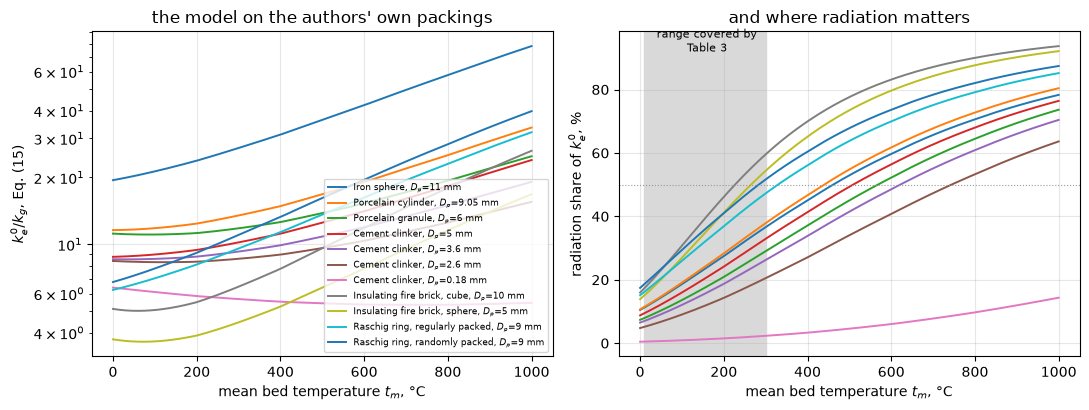
The shaded band on the right panel is the whole temperature range Table 3 covers. The decomposition above puts the void-radiation share of any Table 3 row, and the solid-to-solid term’s share of the contact conductance, at the printed maxima, both well short of half. Where the paper’s conclusions live, 400 °C and above, the same packings run far higher (the table above).
The Raschig rings: a prediction with no free parameter
Yagi & Kunii treat the rings by arguing \(\beta\) from geometry rather than fitting it. For a regular stack, radiation crosses three voids to get from A to B, so \(l_p = \sqrt3 D_p/3\) and \(\beta = 1/\sqrt3\); packed randomly, a ring’s axis lines up with the heat flow about one time in three, giving \(\beta = 1\times(1/3) + (1/\sqrt3)\times(2/3)\). \(\varphi\) and \(\gamma\) are the same for both. The only other difference is the measured voidage, 0.67 against 0.72.
The paper then states, of Figure 17, that the randomly packed data lie about 20 % above the regularly packed data. Nothing in the two \(\beta\) arguments was fitted to that, so it is a genuine prediction.
reg = t4[t4.solid == "Raschig ring, regularly packed"].iloc[0]
ran = t4[t4.solid == "Raschig ring, randomly packed"].iloc[0]
print(f"beta regular = 1/sqrt(3)                    = {reg.beta:.4f}")
print(f"beta random  = 1x(1/3) + (1/sqrt(3))x(2/3)  = {ran.beta:.4f}")
print(f"gamma both   = 1.2/9                        = {reg.gamma:.4f}\n")
for T in (200.0, 400, 600, 800, 1000):
    a_, b_ = sweep(reg, T)[0], sweep(ran, T)[0]
    print(f"  t = {T:6.0f} degC   regular {a_:6.2f}   random {b_:6.2f}   "
          f"random/regular {b_ / a_:.4f}  ({100 * (b_ / a_ - 1):+.1f} %)")
rr = sweep(ran, Tp)[0] / sweep(reg, Tp)[0]
print(f"\nOver 200-1000 degC the model predicts random/regular = "
      f"{100 * (rr.min() - 1):.1f} to {100 * (rr.max() - 1):.1f} %; the paper says 'about 20% greater'.")
METRICS["raschig_random_over_regular_at_600C"] = float(sweep(ran, 600.0)[0] / sweep(reg, 600.0)[0])
METRICS["raschig_random_over_regular_min_pct"] = float(100 * (rr.min() - 1))
METRICS["raschig_random_over_regular_max_pct"] = float(100 * (rr.max() - 1))
beta regular = 1/sqrt(3) = 0.5774
beta random = 1x(1/3) + (1/sqrt(3))x(2/3) = 0.7182
gamma both = 1.2/9 = 0.1333
t = 200 degC regular 8.11 random 9.16 random/regular 1.1294 (+12.9 %)
t = 400 degC regular 11.34 random 13.27 random/regular 1.1705 (+17.1 %)
t = 600 degC regular 16.22 random 19.50 random/regular 1.2024 (+20.2 %)
t = 800 degC regular 23.01 random 28.22 random/regular 1.2260 (+22.6 %)
t = 1000 degC regular 31.97 random 39.76 random/regular 1.2439 (+24.4 %)
Over 200-1000 degC the model predicts random/regular = 12.9 to 24.4 %; the paper says 'about 20% greater'.A second printed defect, and what it costs
Journal page 379 derives \(\gamma\) for the rings:
\(\gamma \doteq l_s/D_p\) = 1.2 mm./9.0 mm. = 0.0134
\(1.2/9.0 = 0.1333\). Table 4 carries the ratio \(1.2/9\) rather than the decimal, so the tabulated calculation is unaffected; only the printed decimal is wrong, by a factor of ten. It is worth measuring anyway, because a reader taking the decimal at face value gets a different answer:
print(f"gamma as the printed ratio 1.2/9.0 : {1.2 / 9.0:.6f}")
print(f"gamma as the printed decimal       : 0.0134   -> off by a factor "
      f"{(1.2 / 9.0) / 0.0134:.2f}\n")
for T in (400.0, 800.0):
    good, bad = sweep(reg, T)[0], sweep(reg, T, gamma=0.0134)[0]
    print(f"  Raschig rings at {T:.0f} degC: ke0/kg {good:.3f} with 1.2/9, "
          f"{bad:.3f} with 0.0134  ({100 * (bad / good - 1):+.2f} %)")
METRICS["gamma_printed_decimal_cost_at_400C_pct"] = float(
    100 * (sweep(reg, 400.0, gamma=0.0134)[0] / sweep(reg, 400.0)[0] - 1))
gamma as the printed ratio 1.2/9.0 : 0.133333
gamma as the printed decimal : 0.0134 -> off by a factor 9.95
Raschig rings at 400 degC: ke0/kg 11.339 with 1.2/9, 12.383 with 0.0134 (+9.21 %)
Raschig rings at 800 degC: ke0/kg 23.014 with 1.2/9, 25.965 with 0.0134 (+12.82 %)The two readings that do not fit, and what they show
The insulating-firebrick curves miss badly at low temperature, and the miss is informative rather than embarrassing. Table 4 prints, for those two rows and no others, both a \(k_s\) (0.20, qualified “at 400 °C const.”) and a \(k_s/k_g\) (4.48). Everywhere else the \(k_s/k_g\) cell is an em dash. Holding \(k_s\) constant is one reading of that row; holding the ratio constant is the other.
KS_OVER_KG_FB = float(t4[t4.solid.str.startswith("Insulating")].ks_over_kg_printed.iloc[0])
print(f"Table 4 prints ks/kg = {KS_OVER_KG_FB} for the two insulating-firebrick rows, and an em dash "
      f"for every other row.\n")
print(f"{'curve':38s} {'t':>7s} {'read':>7s} {'ks=0.20 const':>16s} {'ks/kg=4.48 const':>19s}")
rows = []
for _, r in fc[fb].iterrows():
    row = t4_row(r.solid, r.Dp_mm)
    a = float(eq15_row(row, r.t_C))
    b = float(eq15_row(row, r.t_C, ks=KS_OVER_KG_FB * kg_air(r.t_C)))
    rows.append((100 * (a / r.ke0_over_kg_read - 1), 100 * (b / r.ke0_over_kg_read - 1)))
    print(f"{r.solid + f', Dp={r.Dp_mm:g}':38s} {r.t_C:7.1f} {r.ke0_over_kg_read:7.2f} "
          f"{a:8.2f} ({rows[-1][0]:+6.1f}%) {b:8.2f} ({rows[-1][1]:+6.1f}%)")
ks_const, ratio_const = np.array(rows).T
print(f"\nmean |deviation| over the three firebrick readings: "
      f"{np.abs(ks_const).mean():.1f} % holding ks, {np.abs(ratio_const).mean():.1f} % holding ks/kg.")
METRICS["firebrick_curve_ends_mean_abs_pct_ks_const"] = float(np.abs(ks_const).mean())
METRICS["firebrick_curve_ends_mean_abs_pct_ratio_const"] = float(np.abs(ratio_const).mean())

fbs = t4_row("Insulating fire brick, sphere", 5.0)
g_ratio = lambda T: 100 * (1 - float(eq15(fbs.eps, fbs.beta, fbs.gamma, fbs.phi, fbs.Dp_mm * 1e-3,
                                          KS_OVER_KG_FB * kg_air(T), kg_air(T), 0.0, 0.0))
                           / float(eq15_row(fbs, T, ks=KS_OVER_KG_FB * kg_air(T)))) - 50.0
T_half_ratio = one_root(g_ratio, 0.0, 3000.0)
print(f"\nRadiation reaches half of ke0 for the firebrick spheres at "
      f"{cross_T[('Insulating fire brick, sphere', 5.0)]:.0f} degC holding ks = 0.20, and at "
      f"{T_half_ratio:.0f} degC holding ks/kg = 4.48.\nBoth are far below the 400 degC the paper "
      f"claims, so the conclusion this page reproduces does not turn on the choice.")
METRICS["radiation_half_temp_firebrick_sphere_C_ks_over_kg_const"] = T_half_ratio
Table 4 prints ks/kg = 4.48 for the two insulating-firebrick rows, and an em dash for every other row.
curve t read ks=0.20 const ks/kg=4.48 const
Insulating fire brick, cube, Dp=10 35.4 3.13 5.03 ( +60.8%) 3.34 ( +6.6%)
Insulating fire brick, sphere, Dp=5 35.4 2.44 3.66 ( +50.2%) 2.46 ( +0.9%)
Insulating fire brick, sphere, Dp=5 963.2 15.86 15.74 ( -0.7%) 16.34 ( +3.0%)
mean |deviation| over the three firebrick readings: 37.2 % holding ks, 3.5 % holding ks/kg.
Radiation reaches half of ke0 for the firebrick spheres at 265 degC holding ks = 0.20, and at 233 degC holding ks/kg = 4.48.
Both are far below the 400 degC the paper claims, so the conclusion this page reproduces does not turn on the choice.So the low-temperature end of Figure 16 says the authors held \(k_s/k_g\) fixed at the printed 4.48 for the insulating firebrick, not \(k_s\) at 0.20, which is presumably why that is the only row where Table 4 prints the ratio at all. Insulating firebrick really does conduct roughly twice as well at 400 °C as at room temperature, so the choice is physical as well as arithmetic.
This page keeps \(k_s = 0.20\) as its base case, because that is the column Table 4 labels \(k_s\) and it is what every other packing uses, and reports the firebrick radiation-crossover temperature both ways, 265 °C and 233 °C. The paper’s conclusion being reproduced (“higher than 400 °C”, for poorly conductive solids) is unaffected: both numbers sit well below it, which is the direction that matters.
Validation
Six checks, then a defect-injection table covering every metric this page reports.
V1. Equation (16) is Equation (15) with the radiation switched off
The paper prints both, three lines apart, and never says they are the same equation. They must be: with \(h_{rs} = h_{rv} = 0\) and \(\gamma = 1\), the contact resistance collapses to \(\varphi\) and Eq. (15) becomes Eq. (16). This tests the transcription of both, over random parameters, and a single mis-read term breaks it.
rng = np.random.default_rng(20260805)
N = 20000
P = dict(eps=rng.uniform(0.25, 0.75, N), beta=rng.uniform(0.5, 1.0, N),
         phi=rng.uniform(0.01, 0.20, N), Dp=rng.uniform(1e-4, 2e-2, N),
         ks=rng.uniform(0.1, 50.0, N), kg=rng.uniform(0.02, 0.07, N),
         t=rng.uniform(0.0, 1200.0, N))

a = eq15(P["eps"], P["beta"], np.ones(N), P["phi"], P["Dp"], P["ks"], P["kg"],
         np.zeros(N), np.zeros(N))
b = eq16(P["eps"], P["beta"], P["phi"], P["ks"], P["kg"])
r16 = float(np.max(np.abs(a / b - 1.0)))
print(f"V1  max relative residual Eq.(16) vs Eq.(15)|_(h_r=0, gamma=1) over {N} draws: {r16:.3e}")
METRICS["V1_identity_eq16_from_eq15"] = r16
V1 max relative residual Eq.(16) vs Eq.(15)|_(h_r=0, gamma=1) over 20000 draws: 4.441e-16V2. Equation (14) is the \(k_g \to 0\) limit of Equation (13)
The vacuum form is normalised on \(k_s\) instead of \(k_g\), so the check is that \((k_g/k_s)\times\)Eq. (15) converges to Eq. (14) as \(k_g \to 0\). It is a limit rather than an identity, so the right thing to report is the order, which must be exactly 1, the neglected term is \(k_g/\varphi\) beside \(D_p h_{rs}\).
hs, hv = h_rs(P["t"]), h_rv(P["t"], P["eps"])
scales = np.array([1e-3, 1e-4, 1e-5, 1e-6, 1e-7])
res = []
for s in scales:
    kgs = P["kg"] * s
    lhs = eq15(P["eps"], P["beta"], np.ones(N), P["phi"], P["Dp"], P["ks"], kgs, hs, hv) * kgs / P["ks"]
    rhs = eq14(P["eps"], P["beta"], P["Dp"], P["ks"], hs, hv)
    res.append(float(np.max(np.abs(lhs / rhs - 1.0))))
res = np.array(res)
orders = np.log10(res[:-1] / res[1:]) / np.log10(scales[:-1] / scales[1:])
for s, r in zip(scales, res):
    print(f"  kg scaled by {s:6.0e}: max relative residual {r:.3e}")
print(f"V2  observed order in kg: {orders} -> mean {orders.mean():.4f} (must be 1)")
METRICS["V2_eq14_limit_order"] = float(orders.mean())
METRICS["V2_eq14_residual_at_1e-7"] = float(res[-1])   # the smallest kg scale, 1e-7
kg scaled by 1e-03: max relative residual 1.593e+00
kg scaled by 1e-04: max relative residual 1.593e-01
kg scaled by 1e-05: max relative residual 1.593e-02
kg scaled by 1e-06: max relative residual 1.593e-03
kg scaled by 1e-07: max relative residual 1.593e-04
V2 observed order in kg: [0.99996632 0.99999663 0.99999966 0.99999997] -> mean 1.0000 (must be 1)V3. Equation (13) reassembled from Equations (9)–(12)
Equation (13) is stated as following from the resistance network of Eqs. (9), (10) and (11). Rebuilding it from those, \(q = (k_e^0/\Delta x)\Delta t = \delta(k_s/\Delta x)\Delta t + U_s(1-\epsilon-\delta)\Delta t + U_v\epsilon\Delta t\) with \(1/U_s = (N\Delta x)\{\gamma D_p/k_s + 1/(k_g/(\varphi D_p)+h_{rs})\}\), \(1/U_v = N\Delta x/h_{rv}\) and \(N\Delta x = \Delta x/(\beta D_p)\), is a second, independent transcription of the same physics. The two must agree to machine precision.
delta = rng.uniform(0.0, 1e-6, N)
lhs = eq13_from_network(P["eps"], P["beta"], np.ones(N), P["phi"], P["Dp"], P["ks"],
                        P["kg"], hs, hv, delta)
rhs = (delta * P["ks"] / P["kg"]
       + (1 - P["eps"] - delta) * P["beta"]
       / (1.0 * (P["kg"] / P["ks"]) + 1.0 / ((1 / P["phi"]) + P["Dp"] * hs / P["kg"]))
       + P["eps"] * P["beta"] * P["Dp"] * hv / P["kg"])
r13 = float(np.max(np.abs(lhs / rhs - 1.0)))
print(f"V3  max relative residual, Eq.(13) vs the Eq.(9)-(12) network: {r13:.3e}")
METRICS["V3_eq13_from_network"] = r13
V3 max relative residual, Eq.(13) vs the Eq.(9)-(12) network: 8.882e-16V4. The apparatus constant, from a pymrm solve, and what it does not prove
Discretise the annulus, extract the heat rate, and ask what multiplies \(VI/\Delta t\) to give back \(k_e^0\). With a constant conductivity the problem is linear: one sparse solve per grid. The heat rate goes on a ladder of 100 to 800 cells; its observed orders come from successive differences, its Richardson limit is compared with the closed form \(2\pi k\,\Delta t/\ln(r_o/r_i)\), and the finest difference is compared with the round-off floor of the solve.
It is not a fourth, independent confirmation of the factor of two. solve_annulus returns Qprime = 2.0*np.pi*r_f*flux: the \(2\pi\) is typed in by hand, in the same expression as the disputed constant. construct_div(..., nu=1) enforces only that \(r\,q_r\) is uniform; it never supplies the \(2\pi\), because per unit bed length the conductance is \(2\pi k/\ln(r_o/r_i)\) and the \(2\pi\) is a convention about what “per unit length” means, not a discretisation result. The cell below substitutes \(\pi\) and \(4\pi\) to show exactly that: with \(\pi\) the route returns the printed Eq. (17) constant, which is the thing under dispute.
So V4 is a discretisation check against the closed form it re-implements. The proof that Eq. (17) is a factor of two low is the paper’s own Eq. (19), and that proof needs no decoration.
k0, Tin, Tout = 1.0, 500.0, 100.0
exact = lambda r: Tout + (Tin - Tout) * np.log(R_O / r) / np.log(R_O / R_I)
NS_V4 = (100, 200, 400, 800)        # cells; the profile error is read at 800


def annulus_study(c_ln, nu=1, ns=NS_V4):
    """Constant-k annulus on a ladder of cells: the problem is linear, one solve per grid.

    Returns the heat rate's observed orders (successive differences), its
    Richardson limit against the closed form 2 pi k dT / ln(r_o/r_i), the
    round-off companion (finest difference over cond(A) eps |Q|), the face
    spread of the heat rate, the profile error at 800 cells and the constant
    of Eq. (19) recovered from the 800-cell solve, against ``c_ln``.
    """
    Q, spread = {}, 0.0
    for n in sorted(set(ns) | {800}):
        _, r_c, T, Qp = solve_annulus(n, Tin, Tout, k_const=k0, nu=nu)
        Q[n] = float(Qp[0])
        spread = max(spread, float(np.ptp(Qp) / abs(Qp[0])))
        if n == 800:
            err800 = float(np.max(np.abs(T - exact(r_c))) / (Tin - Tout))
    study = observed_orders(lambda n: Q[n], ns)
    Q_exact = 2 * np.pi * k0 * (Tin - Tout) / np.log(R_O / R_I)
    ops = annulus_operators(ns[-1], Tin, Tout, nu)
    cond = np.linalg.cond((ops["div"] @ (-k0 * ops["grad"])).toarray())
    c_pymrm = k0 * (Tin - Tout) / (Q[800] * L_BED / 0.860)   # kcal/hr -> watts, the paper's factor
    return {"V4_annulus_order_min": float(np.min(study["orders"])),
            "V4_annulus_order_max": float(np.max(study["orders"])),
            "V4_annulus_extrapolated_vs_closed_form": float(abs(study["extrapolated"] / Q_exact - 1)),
            "V4_annulus_roundoff_margin": float(abs(Q[ns[-1]] - Q[ns[-2]])
                                                / (cond * np.finfo(float).eps * abs(Q[ns[-1]]))),
            "V4_annulus_face_spread": spread,
            "V4_annulus_profile_err_n800": err800,
            "V4_pymrm_constant_vs_printed_pct": float(100 * (c_pymrm / 0.743 - 1)),
            "V4_pymrm_vs_closed_form": float(abs(c_pymrm / c_ln - 1)),
            "_Q": Q, "_Q_exact": Q_exact, "_orders": study["orders"], "_c_pymrm": c_pymrm}


V4 = annulus_study(c_two_pi_ln)
print("constant k: linear, one sparse solve per grid")
for n in NS_V4:
    print(f"  n = {n:4d}   heat rate / closed form - 1 = {V4['_Q'][n] / V4['_Q_exact'] - 1:+.3e}")
print(f"observed orders of the heat rate (successive differences): "
      + ", ".join(f"{o:.4f}" for o in V4["_orders"]))
print(f"Richardson limit against the closed form: {V4['V4_annulus_extrapolated_vs_closed_form']:.1e}")
print(f"finest difference over the round-off floor cond(A) eps |Q|: "
      f"{V4['V4_annulus_roundoff_margin']:.0f}")
print(f"heat rate through every face, largest spread over the ladder: "
      f"{V4['V4_annulus_face_spread']:.1e} (the divergence telescopes)")
print(f"profile error at 800 cells, max|T - exact|/dT: {V4['V4_annulus_profile_err_n800']:.3e}")
c_pymrm = V4["_c_pymrm"]
print(f"    constant recovered from the pymrm nu=1 solve: {c_pymrm:.6f}")
print(f"    printed Eq. (19):                             0.743   "
      f"({100 * (c_pymrm / 0.743 - 1):+.4f} %)")
print(f"    closed form with 2 pi l and exact ln:         {c_two_pi_ln:.6f}   "
      f"(the 800-cell solve is {V4['V4_pymrm_vs_closed_form']:.1e} from it)")
print("\nWhere that 2 pi comes from: it is TYPED, not solved for. Re-running the same solve with")
print("the prefactor changed and nothing else:")
for lab, pref in [("1.0*np.pi (Eq. 17 as printed)", 1.0), ("2.0*np.pi (correct)", 2.0),
                  ("4.0*np.pi", 4.0)]:
    _, _, _, Qz = solve_annulus(800, Tin, Tout, k_const=k0)
    Qz = Qz / (2.0 * np.pi) * (pref * np.pi)
    print(f"    {lab:30s} -> constant {k0 * (Tin - Tout) / (Qz[0] * L_BED / 0.860):.6f}")
print("So V4 tests the DISCRETISATION, not the geometry constant. Only the nu=1 -> nu=0")
print("break row tests the geometry.")
METRICS.update({k: v for k, v in V4.items() if not k.startswith("_")})
constant k: linear, one sparse solve per grid
n = 100 heat rate / closed form - 1 = +2.177e-05
n = 200 heat rate / closed form - 1 = +5.713e-06
n = 400 heat rate / closed form - 1 = +1.463e-06
n = 800 heat rate / closed form - 1 = +3.701e-07
observed orders of the heat rate (successive differences): 1.9176, 1.9595
Richardson limit against the closed form: 8.1e-09
finest difference over the round-off floor cond(A) eps |Q|: 15456
heat rate through every face, largest spread over the ladder: 4.0e-12 (the divergence telescopes)
profile error at 800 cells, max|T - exact|/dT: 1.134e-07
constant recovered from the pymrm nu=1 solve: 0.744188
printed Eq. (19): 0.743 (+0.1599 %)
closed form with 2 pi l and exact ln: 0.744188 (the 800-cell solve is 3.7e-07 from it)
Where that 2 pi comes from: it is TYPED, not solved for. Re-running the same solve with
the prefactor changed and nothing else:
1.0*np.pi (Eq. 17 as printed) -> constant 1.488376
2.0*np.pi (correct) -> constant 0.744188
4.0*np.pi -> constant 0.372094
So V4 tests the DISCRETISATION, not the geometry constant. Only the nu=1 -> nu=0
break row tests the geometry.The discretised cylindrical solve lands on the exact-\(\ln\) closed form to its printed discretisation error, and the printed 0.743 sits below it by the printed deviation, which is the paper’s rounding of \(\ln 10\) to 2.3.
V5. Emissivity, the constant the paper never prints, and the one evaluation point everything else sits on
\(p\) enters Eqs. (7) and (8) and is nowhere given. Every other calculation on this page uses \(p = 1\), and at \(p = 1\) the two coefficients are numerically identical: Eq. (7)’s \(p/(2-p)\) is 1, Eq. (8)’s \(1 + [\epsilon/2(1-\epsilon)](1-p)/p\) is 1, and both collapse to the black-body \(0.1952\,(T/100)^3\) independently of \(\epsilon\). That makes every other metric on this page blind to the entire emissivity structure of both equations: Eqs. (7) and (8) could be exchanged wholesale and, before the V5 family below existed, exactly one metric of 53 would have noticed, and that one was V5 itself, the output of the assumption under test.
This is the A1.8 exposure, every check standing at one evaluation point of a branched model. So V5 evaluates away from that point as well, and the break table below carries three injections that attack the \(p\)-structure directly.
print("iron spheres, Table 4 parameters")
base = None
for p in (1.0, 0.9, 0.8, 0.6):
    v = [float(sweep(iron, T, p=p)[0]) for T in (400.0, 1000.0)]
    if base is None:
        base = v
    print(f"  p = {p:.1f}:  ke0/kg = {v[0]:6.2f} at 400 degC ({100 * (v[0] / base[0] - 1):+5.1f} %), "
          f"{v[1]:6.2f} at 1000 degC ({100 * (v[1] / base[1] - 1):+5.1f} %)")
p08 = float(sweep(iron, 1000.0, p=0.8)[0])
METRICS["V5_emissivity_p08_vs_p10_at_1000C_pct"] = float(100 * (p08 / base[1] - 1))
print(f"\nA plausible p = 0.8 moves the 1000 degC value by "
      f"{100 * (p08 / base[1] - 1):+.1f} %. Every radiation number on this page carries that.")

print(f"\nThe collapse at p = 1, and what it hides. h_rs/h_rv at eps = 0.40:")
for p in (1.0, 0.8, 0.6):
    print(f"  p = {p:.1f}:  h_rs = {h_rs(500.0, p):.5f}   h_rv = {h_rv(500.0, 0.40, p):.5f}   "
          f"ratio {h_rs(500.0, p) / h_rv(500.0, 0.40, p):.5f}")
METRICS["V5_hrs_over_hrv_at_p06_eps040"] = float(h_rs(500.0, 0.6) / h_rv(500.0, 0.40, 0.6))
METRICS["V5_hrs_p06_over_blackbody"] = float(h_rs(500.0, 0.6) / h_rs(500.0, 1.0))
METRICS["V5_hrv_eps_spread_at_p06_pct"] = float(
    100 * (h_rv(500.0, 0.30, 0.6) / h_rv(500.0, 0.50, 0.6) - 1))
METRICS["V5_emissivity_p06_vs_p10_at_1000C_pct"] = float(
    100 * (float(sweep(iron, 1000.0, p=0.6)[0]) / base[1] - 1))
print(f"  Eq. (7)'s p-group alone at p = 0.6      : {METRICS['V5_hrs_p06_over_blackbody']:.5f} "
      f"(= 0.6/1.4)")
print(f"  Eq. (8)'s eps-group, 0.30 vs 0.50 at p = 0.6: "
      f"{METRICS['V5_hrv_eps_spread_at_p06_pct']:+.2f} % -- exactly zero at p = 1")
iron spheres, Table 4 parameters
p = 1.0: ke0/kg = 31.18 at 400 degC ( +0.0 %), 78.07 at 1000 degC ( +0.0 %)
p = 0.9: ke0/kg = 29.50 at 400 degC ( -5.4 %), 71.35 at 1000 degC ( -8.6 %)
p = 0.8: ke0/kg = 28.03 at 400 degC (-10.1 %), 65.29 at 1000 degC (-16.4 %)
p = 0.6: ke0/kg = 25.47 at 400 degC (-18.3 %), 54.42 at 1000 degC (-30.3 %)
A plausible p = 0.8 moves the 1000 degC value by -16.4 %. Every radiation number on this page carries that.
The collapse at p = 1, and what it hides. h_rs/h_rv at eps = 0.40:
p = 1.0: h_rs = 90.16091 h_rv = 90.16091 ratio 1.00000
p = 0.8: h_rs = 60.10727 h_rv = 83.22546 ratio 0.72222
p = 0.6: h_rs = 38.64039 h_rv = 73.76802 ratio 0.52381
Eq. (7)'s p-group alone at p = 0.6 : 0.42857 (= 0.6/1.4)
Eq. (8)'s eps-group, 0.30 vs 0.50 at p = 0.6: +16.67 % -- exactly zero at p = 1V6. Defect injection
recompute() below rebuilds every number of the sections above, and of the reduction-bias section further down, from the data, with optional defects passed as arguments: a mis-read constant, a swapped equation group, a shifted column, the Cartesian divergence, a loose stopping rule. An assertion checks that it reproduces the narrative cells before any defect goes in. The claims each defect fails are decided in the Claims section at the end, once every claim is registered.
Every row perturbs an input and watches a number move, so no row can catch a baseline that is wrong rather than insensitive. Section 4’s three identical deviations are the worked example: they look like confirmation and are one number printed twice. The defence is a second computation from an independent source, The curves the authors drew, which compares this page’s Eq. (15) against numbers the paper printed and this page never otherwise touches.
def recompute(ell_factor=2.0, Di=DI_M, kg_flat=None, hr_scale=1.0, p=1.0,
              gamma_ring=None, beta_random=None, ks_fine=None, reciprocal=False,
              rings_ordinary=False, exp_shift=False, t1_shift=False, nu=1, eq15_kind="ok",
              eq13_kind="ok", drop_phi_pair=None, phi_beta=1.0, phi_gamma=1.0,
              swap_hr=False, hrs_kind="ok", hrv_kind="ok", t1_ref15_raschig=False,
              f12_pad=0.0, method="newton", tol=1e-8, read_err=None):
    """Recompute EVERY published metric under an optional injected defect.

    Called once with no arguments for the baseline, then once per row of the break
    table.  Keeping one function means a metric cannot quietly escape the table.
    """
    M = {}
    kgf = (lambda t: np.full_like(np.asarray(t, float), kg_air(kg_flat))) if kg_flat is not None else kg_air

    # --- variant radiation coefficients, for the p-structure injections ----------
    def HS(t_C, pp=None):
        pp = p if pp is None else pp
        g = (2*pp/(1+pp)) if hrs_kind == "pgroup2" else (pp/(2.0 - pp))
        return hr_scale * SIG4 * g * ((t_C + 273.0)/100.0)**3

    def HV(t_C, eps, pp=None):
        pp = p if pp is None else pp
        eg = ((1-eps)/(2*eps)) if hrv_kind == "epsinv" else (eps/(2*(1-eps)))
        return hr_scale * SIG4 / (1.0 + eg*(1-pp)/pp) * ((t_C + 273.0)/100.0)**3

    if swap_hr:
        HS, HV = (lambda t, pp=None, _v=HV: _v(t, 0.40, pp)), (lambda t, e, pp=None, _s=HS: _s(t, pp))

    # --- variant equation forms, for the identity checks -------------------------
    def e15(eps, beta, gamma, phi, Dp, ks, kg, hrs, hrv):
        if eq15_kind == "signflip":
            return beta*(1-eps)/(gamma*(kg/ks) - 1/((1/phi)+Dp*hrs/kg)) + eps*beta*Dp*hrv/kg
        if eq15_kind == "phiinv":
            return eq15(eps, beta, gamma, 1.0/phi, Dp, ks, kg, hrs, hrv)
        if eq15_kind == "nogamma":
            return beta*(1-eps)/(1/((1/phi)+Dp*hrs/kg)) + eps*beta*Dp*hrv/kg
        return eq15(eps, beta, gamma, phi, Dp, ks, kg, hrs, hrv)

    # --- A. the apparatus constants ---------------------------------------------
    c_pf = 0.860*2.3*np.log10(D0_M/Di)/(1.0*np.pi*L_BED)
    c_ok = 0.860*2.3*np.log10(D0_M/Di)/(ell_factor*np.pi*L_BED)
    c_ln = 0.860*np.log(D0_M/Di)/(ell_factor*np.pi*L_BED)
    M["eq17_as_printed_over_eq19_ratio"] = c_pf/0.743
    M["eq19_constant_2pi_vs_printed_pct"] = 100*(c_ok/0.743 - 1)
    M["eq19_constant_exact_ln_vs_printed_pct"] = 100*(c_ln/0.743 - 1)
    M["table4_ks_over_kg_roundtrip_pct"] = float(100*(0.20/kgf(400.0)/4.48 - 1))

    # --- B. Table 1 --------------------------------------------------------------
    shaped = t1.solid.str.contains("Raschig|saddle", case=False)
    rng_m = t1.solid.str.contains("Raschig", case=False)
    o = ab if rings_ordinary else ab[~shaped]
    kfb = KS_OVER_KG_FB
    M["alpha_beta_ordinary_mean"] = float(o.mean())
    M["alpha_beta_ordinary_in_printed_band_frac"] = float(
        ((o >= 0.1-1e-9) & (o <= 0.14+1e-9)).sum()/len(o))
    M["alpha_beta_ring_over_ordinary_ratio"] = float(ab[rng_m].mean()/o.mean())
    M["alpha_beta_theory_over_observed_lower"] = float(0.179*0.82/o.mean())
    t1x = t1.copy()
    if t1_shift:
        t1x["ke0_over_kg"] = t1x.ke0_over_kg.shift(1)
    _sd = t1x.dropna(subset=["ke0_over_kg"])
    M["static_dynamic_crossover_PeM_median"] = float(
        (_sd.ke0_over_kg.astype(float)/_sd.alpha_beta.astype(float)).median())

    # --- C. the paper's own comparison ------------------------------------------
    t3x = t3.copy()
    if exp_shift:
        t3x["exp_ke0_over_kg"] = t3x.exp_ke0_over_kg.shift(1)
    hv_ = t3x[t3x.exp_ke0_over_kg.notna()]
    dv = (100*(hv_.exp_ke0_over_kg/hv_.calcd_ke0_over_kg - 1) if reciprocal
          else 100*(hv_.calcd_ke0_over_kg/hv_.exp_ke0_over_kg - 1))
    M["paper_calcd_vs_exp_mean_abs_pct"] = float(dv.abs().mean())
    M["paper_calcd_vs_exp_bias_pct"] = float(dv.mean())
    M["paper_calcd_vs_exp_worst_abs_pct"] = float(dv.abs().max())
    M["paper_calcd_vs_exp_mean_abs_pct_no_celite"] = float(dv[hv_.reference != 5].abs().mean())
    M["paper_calcd_vs_exp_bias_se_pct"] = float(dv.std(ddof=1) / np.sqrt(len(dv)))
    if t1_ref15_raschig:      # pair reference 15 by ROW ORDER instead of by packing
        t1x = pd.concat([t1x[t1x.reference != 15],
                         t1x[(t1x.reference == 15) & t1x.solid.str.contains("Raschig")]])
    cx = cross_table(t1x, t3x)
    M["table1_vs_table3_exp_max_abs_pct"] = float(cx.dev_pct.abs().max())
    M["table1_vs_table3_identical_rows"] = float((cx.dev_pct.abs() < 1e-12).sum())
    M["table1_vs_table3_daggered_rows"] = float(cx.daggered.sum())

    # --- D. phi inversion, decomposition, deletion -------------------------------
    ww = t3.copy()
    ww["kg"] = np.where(air, kgf(t3.temp_C.values), np.nan)

    def fw(row, phi, **kw):
        eps, ks, kg = row.eps, row.ks_kcal_m_hr_C, row.kg
        if np.isnan(row.Dp_mm):
            return eq16(eps, phi_beta, phi, ks, kg)
        Dp = row.Dp_mm*1e-3
        hs_ = 0.0 if kw.get("drop_hrs") else HS(row.temp_C)
        hv2 = 0.0 if kw.get("drop_hrv") else HV(row.temp_C, eps)
        return e15(eps, kw.get("beta", phi_beta), kw.get("gamma", phi_gamma),
                   phi, Dp, ks, kg, hs_, hv2)

    def inv_row(row, **kw):
        eps, ks, kg, tgt = row.eps, row.ks_kcal_m_hr_C, row.kg, row.calcd_ke0_over_kg
        if np.isnan(kg):
            return np.nan
        if np.isnan(row.Dp_mm):
            return (1.0 - eps)/tgt - kg/ks
        Dp = row.Dp_mm*1e-3
        hs_ = 0.0 if kw.get("drop_hrs") else HS(row.temp_C)
        hv2 = 0.0 if kw.get("drop_hrv") else HV(row.temp_C, eps)
        res = tgt - eps*Dp*hv2/kg
        if res <= 0:
            return np.nan
        c = (1.0 - eps)/res - phi_gamma*kg/ks
        if c <= 0 or (1.0/c - Dp*hs_/kg) <= 0:
            return np.nan
        return 1.0/(1.0/c - Dp*hs_/kg)

    ww["phi_implied"] = [inv_row(r) for _, r in ww.iterrows()]
    wa_ = ww[air]
    a40 = wa_[np.isclose(wa_.eps, 0.40)].phi_implied.dropna()
    a40n5 = wa_[np.isclose(wa_.eps, 0.40) & (wa_.reference != 5)].phi_implied.dropna()
    M["phi_implied_spread_at_eps040"] = float(a40.max()/a40.min())
    M["phi_implied_spread_at_eps040_no_celite"] = float(a40n5.max()/a40n5.min())
    M["phi_implied_median_at_eps040"] = float(a40.median())

    pr = t4[["eps", "phi"]].drop_duplicates()
    pr = pr[pr.eps <= 0.60].sort_values("eps")
    if drop_phi_pair is not None:
        pr = pr[~np.isclose(pr.eps, drop_phi_pair)]
    cf = np.polyfit(pr.eps, np.log(pr.phi), 1)
    pl = lambda e: np.exp(np.polyval(cf, e))
    M["phi_line_at_eps040_vs_printed_0034_pct"] = float(100*(pl(0.40)/0.034 - 1))
    fwv = np.array([fw(r, pl(r.eps)) for _, r in wa_.iterrows()])
    M["forward_from_phi_line_vs_calcd_mean_abs_pct"] = float(
        np.mean(np.abs(100*(fwv/wa_.calcd_ke0_over_kg.values - 1))))
    hem = wa_.exp_ke0_over_kg.notna().values
    M["forward_from_phi_line_vs_exp_mean_abs_pct"] = float(
        np.mean(np.abs(100*(fwv[hem]/wa_.exp_ke0_over_kg.values[hem] - 1))))

    dd2 = wa_[wa_.Dp_mm.notna()]
    vr, hr_c = [], []
    for _, r in dd2.iterrows():
        kg, ks, eps, Dp = r.kg, r.ks_kcal_m_hr_C, r.eps, r.Dp_mm*1e-3
        hs_, hv2 = HS(r.temp_C), HV(r.temp_C, eps)
        vr.append(100*(eps*Dp*hv2/kg)/r.calcd_ke0_over_kg)
        hr_c.append(100*(Dp*hs_/kg)/((1/r.phi_implied) + Dp*hs_/kg))
    M["table3_max_void_radiation_share_pct"] = float(np.max(vr))
    M["table3_max_hrs_share_of_contact_pct"] = float(np.max(hr_c))

    def cm(row, **kw):
        tgt = row.calcd_ke0_over_kg
        ends = [fw(row, 1e-4, **kw), fw(row, 1.0, **kw)]
        if (ends[0] - tgt)*(ends[1] - tgt) <= 0:
            return 0.0
        return 100*min(abs(v/tgt - 1) for v in ends)

    def pn(row, **kw):
        f = lambda ph: fw(row, ph, **kw) - row.calcd_ke0_over_kg
        roots = find_roots(f, 1e-8, 10.0, log=True, xtol=1e-14)["roots"]
        if len(roots) > 1:
            raise ValueError(f"more than one phi reproduces the row: {roots}")
        return float(roots[0]) if roots else np.nan      # no phi in the bracket: unmatched

    for key, kw in [("hrs", dict(drop_hrs=True)), ("hrv", dict(drop_hrv=True)),
                    ("gamma", dict(gamma=0.0)), ("control_beta_half", dict(beta=0.5*phi_beta))]:
        sh_ = np.array([cm(r, **kw) for _, r in dd2.iterrows()])
        M[f"delete_{key}_rows_unmatched"] = float((sh_ > 1e-9).sum())
        if key == "hrv":
            M["delete_hrv_worst_shortfall_pct"] = float(sh_.max())
        if key == "control_beta_half":
            M["delete_control_beta_half_worst_shortfall_pct"] = float(sh_.max())
        if key in ("hrs", "gamma"):
            nd_ = np.array([pn(r, **kw) for _, r in dd2.iterrows()])
            M[f"delete_{key}_max_phi_needed"] = (float(np.nanmax(nd_)) if np.isfinite(nd_).any()
                                                 else np.nan)
            M[f"delete_{key}_rows_phi_above_printed"] = float(np.nansum(nd_ > PHI_PRINTED_HI))
            if key == "gamma":
                M["delete_gamma_rows_off_fig9_axis"] = float(np.nansum(nd_ > PHI_FIG9_TOP))
    ph_ = np.array([inv_row(r, drop_hrs=True) for _, r in dd2.iterrows()])
    bk_ = np.array([fw(r, q, drop_hrs=True) for (_, r), q in zip(dd2.iterrows(), ph_)])
    M["delete_hrs_exact_reproduction_resid"] = float(
        np.max(np.abs(bk_/dd2.calcd_ke0_over_kg.values - 1)))
    M["delete_hrs_max_phi_shift_pct"] = float(
        np.nanmax(np.abs(100*(ph_/dd2.phi_implied.values - 1))))

    # --- E. Table 4 sweeps -------------------------------------------------------
    def swp(row, T, gg=None, bb=None, kks=None):
        kg = kgf(T)
        Dp = row.Dp_mm*1e-3
        ks = row.ks_kcal_m_hr_C if kks is None else kks
        g = (row.gamma if gg is None else gg)
        b = (row.beta if bb is None else bb)
        hs_, hv2 = HS(T), HV(T, row.eps)
        full = e15(row.eps, b, g, row.phi, Dp, ks, kg, hs_, hv2)
        nor = e15(row.eps, b, g, row.phi, Dp, ks, kg, 0.0, 0.0)
        return full, 100*(1 - nor/full)

    for key, (nm, dp) in {"iron_sphere": ("Iron sphere", 11.0),
                          "firebrick_sphere": ("Insulating fire brick, sphere", 5.0),
                          }.items():
        rr_ = t4[(t4.solid == nm) & np.isclose(t4.Dp_mm, dp)].iloc[0]
        kks = None
        g_ = lambda T: swp(rr_, T, kks=kks)[1] - 50.0
        try:
            M[f"radiation_half_temp_{key}_C"] = one_root(g_, 0.0, 3000.0)
        except ValueError:                      # no single crossing on 0 to 3000 degC
            M[f"radiation_half_temp_{key}_C"] = np.nan
    _rf = t4[(t4.solid == "Cement clinker") & np.isclose(t4.Dp_mm, 0.18)].iloc[0]
    M["radiation_share_fine_clinker_at_1200C_pct"] = float(
        swp(_rf, kgt.temp_C.max(), kks=ks_fine)[1])
    for key, (nm, dp) in {"fine_clinker": ("Cement clinker", 0.18),
                          "coarse_clinker": ("Cement clinker", 5.0),
                          "iron_sphere": ("Iron sphere", 11.0)}.items():
        rr_ = t4[(t4.solid == nm) & np.isclose(t4.Dp_mm, dp)].iloc[0]
        kks = ks_fine if (key == "fine_clinker" and ks_fine is not None) else None
        v = swp(rr_, Tp, kks=kks)[0]
        M[f"{key}_spread_pct_200_1000C"] = float(100*(v.max()/v.min() - 1))
    br = beta_random if beta_random is not None else ran.beta
    gr = gamma_ring if gamma_ring is not None else reg.gamma
    rat = swp(ran, Tp, gg=gr, bb=br)[0]/swp(reg, Tp, gg=gr)[0]
    M["raschig_random_over_regular_at_600C"] = float(
        swp(ran, 600.0, gg=gr, bb=br)[0]/swp(reg, 600.0, gg=gr)[0])
    M["raschig_random_over_regular_min_pct"] = float(100*(rat.min() - 1))
    M["raschig_random_over_regular_max_pct"] = float(100*(rat.max() - 1))
    M["gamma_printed_decimal_cost_at_400C_pct"] = float(
        100*(swp(reg, 400.0, gg=0.0134)[0]/swp(reg, 400.0, gg=gr)[0] - 1))
    _ka = dict(eps=iron.eps, beta=iron.beta, gamma=iron.gamma, phi=iron.phi,
               Dp=iron.Dp_mm*1e-3, ks=iron.ks_kcal_m_hr_C, kg=kgf(1000.0))
    _k10 = e15(_ka["eps"], _ka["beta"], _ka["gamma"], _ka["phi"], _ka["Dp"], _ka["ks"], _ka["kg"],
               HS(1000.0), HV(1000.0, iron.eps))
    _k08 = e15(_ka["eps"], _ka["beta"], _ka["gamma"], _ka["phi"], _ka["Dp"], _ka["ks"], _ka["kg"],
               HS(1000.0, 0.8), HV(1000.0, iron.eps, 0.8))
    _k06 = e15(_ka["eps"], _ka["beta"], _ka["gamma"], _ka["phi"], _ka["Dp"], _ka["ks"], _ka["kg"],
               HS(1000.0, 0.6), HV(1000.0, iron.eps, 0.6))
    M["V5_emissivity_p08_vs_p10_at_1000C_pct"] = float(100*(_k08/_k10 - 1))
    M["V5_emissivity_p06_vs_p10_at_1000C_pct"] = float(100*(_k06/_k10 - 1))
    M["V5_hrs_over_hrv_at_p06_eps040"] = float(HS(500.0, 0.6)/HV(500.0, 0.40, 0.6))
    M["V5_hrs_p06_over_blackbody"] = float(HS(500.0, 0.6)/HS(500.0, 1.0))
    M["V5_hrv_eps_spread_at_p06_pct"] = float(100*(HV(500.0, 0.30, 0.6)/HV(500.0, 0.50, 0.6) - 1))

    # --- E2. the authors' own printed theoretical curves --------------------------
    def swp_row(row, T, ks=None, bb=None):
        kg = kgf(T)
        return e15(row.eps, row.beta if bb is None else bb, row.gamma, row.phi,
                   row.Dp_mm*1e-3, row.ks_kcal_m_hr_C if ks is None else ks, kg,
                   HS(T), HV(T, row.eps))

    fcx, fbm = fcurves, fcurves.solid.str.startswith("Insulating")
    bof = lambda r: (float(r.beta_curve) if np.isfinite(r.beta_curve) else None)
    dvc = np.array([100*(float(swp_row(t4_row(r.solid, r.Dp_mm), r.t_C, bb=bof(r)))
                         / r.ke0_over_kg_read - 1) for _, r in fcx[~fbm].iterrows()])
    M["fig13to17_curve_ends_mean_abs_pct"] = float(np.abs(dvc).mean())
    M["fig13to17_curve_ends_worst_abs_pct"] = float(np.abs(dvc).max())
    def _c08(r):
        rw = t4_row(r.solid, r.Dp_mm)
        b_ = bof(r)
        return float(e15(rw.eps, rw.beta if b_ is None else b_, rw.gamma, rw.phi, r.Dp_mm*1e-3,
                         rw.ks_kcal_m_hr_C, kgf(r.t_C), HS(r.t_C, 0.8), HV(r.t_C, rw.eps, 0.8)))

    dv08 = np.array([100*(_c08(r)/r.ke0_over_kg_read - 1) for _, r in fcx[~fbm].iterrows()])
    M["fig13to17_curve_ends_mean_abs_pct_at_p08"] = float(np.abs(dv08).mean())

    def _dev_p(pp, off=0.0):
        out = []
        for _, r in fcx[~fbm].iterrows():
            rw, b_ = t4_row(r.solid, r.Dp_mm), bof(r)
            out.append(100*(float(e15(rw.eps, rw.beta if b_ is None else b_, rw.gamma, rw.phi,
                                      r.Dp_mm*1e-3, rw.ks_kcal_m_hr_C, kgf(r.t_C), HS(r.t_C, pp),
                                      HV(r.t_C, rw.eps, pp)))/(r.ke0_over_kg_read + off) - 1))
        return np.array(out)

    rde = 100*(CURVE_READ_ERR if read_err is None else read_err)/fcx.loc[~fbm, "ke0_over_kg_read"].values
    d09_ = _dev_p(0.9)
    M["fig13to17_reading_error_mean_pct"] = float(rde.mean())
    M["fig13to17_curve_ends_se_pct"] = float(dvc.std(ddof=1)/np.sqrt(len(dvc)))
    M["fig13to17_curve_ends_positive_count"] = float((dvc > 0).sum())
    M["fig13to17_within_reading_error_p10"] = float((np.abs(dvc) <= rde).sum())
    M["fig13to17_within_reading_error_p09"] = float((np.abs(d09_) <= rde).sum())
    M["fig13to17_mean_dev_pct_at_p09"] = float(d09_.mean())
    M["fig13to17_mean_dev_pct_at_p08"] = float(dv08.mean())
    try:
        M["fig13to17_p_zero_mean_dev"] = one_root(lambda pp: _dev_p(pp).mean(), 0.5, 1.0, n_scan=11)
    except ValueError:                          # no single zero of the mean on 0.5 <= p <= 1
        M["fig13to17_p_zero_mean_dev"] = np.nan
    _roff = CURVE_READ_ERR if read_err is None else read_err
    for _k, _o in (("lo", -_roff), ("hi", _roff)):    # every reading shifted by one offset
        try:
            M[f"fig13to17_p_zero_offset_{_k}"] = one_root(
                lambda pp, o=_o: _dev_p(pp, o).mean(), 0.5, 1.0, n_scan=11)
        except ValueError:
            M[f"fig13to17_p_zero_offset_{_k}"] = np.nan
    fk = np.array([[100*(float(swp_row(t4_row(r.solid, r.Dp_mm), r.t_C))/r.ke0_over_kg_read - 1),
                    100*(float(swp_row(t4_row(r.solid, r.Dp_mm), r.t_C, ks=kfb*kgf(r.t_C)))
                         / r.ke0_over_kg_read - 1)] for _, r in fcx[fbm].iterrows()])
    M["firebrick_curve_ends_mean_abs_pct_ks_const"] = float(np.abs(fk[:, 0]).mean())
    M["firebrick_curve_ends_mean_abs_pct_ratio_const"] = float(np.abs(fk[:, 1]).mean())
    _fbs = t4_row("Insulating fire brick, sphere", 5.0)
    _gr = lambda T: 100*(1 - float(e15(_fbs.eps, _fbs.beta, _fbs.gamma, _fbs.phi,
                                       _fbs.Dp_mm*1e-3, kfb*kgf(T), kgf(T), 0.0, 0.0))
                         / float(swp_row(_fbs, T, ks=kfb*kgf(T)))) - 50.0
    try:
        M["radiation_half_temp_firebrick_sphere_C_ks_over_kg_const"] = one_root(_gr, 0.0, 3000.0)
    except ValueError:
        M["radiation_half_temp_firebrick_sphere_C_ks_over_kg_const"] = np.nan

    # --- F. the printed identities ----------------------------------------------
    aa = e15(P["eps"], P["beta"], np.ones(N), P["phi"], P["Dp"], P["ks"], P["kg"],
             np.zeros(N), np.zeros(N))
    M["V1_identity_eq16_from_eq15"] = float(np.max(np.abs(aa/b - 1.0)))
    rs_ = []
    for sc in scales:
        kgs = P["kg"]*sc
        lh = e15(P["eps"], P["beta"], np.ones(N), P["phi"], P["Dp"], P["ks"], kgs, hs, hv)*kgs/P["ks"]
        rs_.append(float(np.max(np.abs(lh/eq14(P["eps"], P["beta"], P["Dp"], P["ks"], hs, hv) - 1))))
    rs_ = np.array(rs_)
    M["V2_eq14_limit_order"] = float(np.mean(np.log10(rs_[:-1]/rs_[1:])
                                             / np.log10(scales[:-1]/scales[1:])))
    M["V2_eq14_residual_at_1e-7"] = float(rs_[-1])
    # beta enters eq13_from_network only through N = 1/(beta Dp); beta -> 1 injects N = 1/Dp
    beta_N = P["beta"] if eq13_kind == "ok" else np.ones(N)
    lh13 = eq13_from_network(P["eps"], beta_N, np.ones(N), P["phi"], P["Dp"],
                             P["ks"], P["kg"], hs, hv, delta)
    M["V3_eq13_from_network"] = float(np.max(np.abs(lh13/rhs - 1.0)))

    # --- G. the annulus ----------------------------------------------------------
    M.update({k: v for k, v in annulus_study(c_ln, nu=nu).items() if not k.startswith("_")})

    # --- H. the reduction bias ---------------------------------------------------
    def ke0_i(T):
        kg = kgf(T)
        return kg*e15(iron.eps, iron.beta, iron.gamma, iron.phi, iron.Dp_mm*1e-3,
                      iron.ks_kcal_m_hr_C, kg, HS(T),
                      HV(T, iron.eps))
    T_MID = 500.0
    bi, ns_, kid = [], [], []
    for dT in (50.0, 100.0, 200.0, 400.0, 600.0, 800.0):
        Ti_, To_ = T_MID + dT/2, T_MID - dT/2
        rf_, rc_, T_, Q_ = solve_annulus(400, Ti_, To_, kfun=ke0_i, nu=nu, method=method, tol=tol)
        vol = 2*np.pi*rc_*np.diff(rf_)
        vol /= vol.sum()
        tm_ = float(np.sum(vol*T_))
        ka = float(Q_[0]/(2*np.pi)*np.log(R_O/R_I)/dT)
        Tg_ = np.linspace(To_, Ti_, 20001)
        kid.append(abs(ka/float(np.trapezoid(ke0_i(Tg_), Tg_)/dT) - 1))
        bi.append(100*(ka/ke0_i(tm_) - 1))
        ns_.append(float(np.max(np.abs(T_ - np.polyval(np.polyfit(rc_, T_, 1), rc_)))/dT))
    _, rcc, Tcc, _ = solve_annulus(400, T_MID + 400, T_MID - 400, k_const=1.0, nu=nu)
    volc = 2*np.pi*rcc*np.diff(np.linspace(R_I, R_O, 401))
    volc /= volc.sum()
    M["reduction_bias_swept_min_pct"] = float(np.min(bi))
    M["reduction_bias_swept_max_pct"] = float(np.max(bi))
    M["k_app_vs_closed_form_identity"] = float(np.max(kid))
    M["tm_fraction_of_dT_constant_k"] = float((T_MID + 400 - np.sum(volc*Tcc))/800.0)
    M["nonstraightness_constant_k"] = float(
        np.max(np.abs(Tcc - np.polyval(np.polyfit(rcc, Tcc, 1), rcc)))/800.0)
    M["nonstraightness_varK_swept_min"] = float(np.min(ns_))

    # --- H2. the same, at the FIVE temperature drops Figure 12 actually shows -----
    bi12, ns12, dT12, sp12 = [], [], [], []
    for _, q in f12.iterrows():
        Ti_, To_ = float(q.t_inside_C) + f12_pad, float(q.t_outside_C) - f12_pad
        dT = Ti_ - To_
        dT12.append(dT)
        rf_, rc_, T_, Q_ = solve_annulus(400, Ti_, To_, kfun=ke0_i, nu=nu, method=method, tol=tol)
        sp12.append(float(np.ptp(Q_)/abs(Q_[0])))
        vol = 2*np.pi*rc_*np.diff(rf_)
        vol /= vol.sum()
        ka = float(Q_[0]/(2*np.pi)*np.log(R_O/R_I)/dT)
        bi12.append(100*(ka/ke0_i(float(np.sum(vol*T_))) - 1))
        ns12.append(float(np.max(np.abs(T_ - np.polyval(np.polyfit(rc_, T_, 1), rc_)))/dT))
    M["fig12_dT_min_C"] = float(np.min(dT12))
    M["fig12_dT_max_C"] = float(np.max(dT12))
    M["reduction_bias_min_pct"] = float(np.min(bi12))
    M["reduction_bias_max_pct"] = float(np.max(bi12))
    M["nonstraightness_varK_at_fig12_max"] = float(np.max(ns12))
    M["straightness_factor_at_fig12_min"] = float(
        M["nonstraightness_constant_k"]/np.max(ns12))
    M["annulus_varK_face_spread_max"] = float(np.max(sp12))
    return M


BASE = recompute()
drift = {k: (METRICS[k], BASE[k]) for k in BASE
         if k in METRICS and not np.isclose(METRICS[k], BASE[k], rtol=1e-8, atol=1e-12)}
print(f"recompute() rebuilds {len(BASE)} metrics; {len(METRICS)} narrative metrics exist at this "
      f"point in the notebook, and {len(drift)} of them differ by more than 1e-8 relative: {drift}")
assert not drift, "the break-table recompute has drifted from the narrative cells"
missing = sorted(set(BASE) - set(METRICS))
print(f"{len(missing)} metric(s) are defined by recompute() but not yet by a narrative cell: "
      f"{missing}\nThey are checked against their narrative cells at the END of "
      f"'What pymrm adds', so the assertion covers all {len(BASE)}.")
METRICS.update(BASE)   # single source of truth from here on
recompute() rebuilds 94 metrics; 81 narrative metrics exist at this point in the notebook, and 0 of them differ by more than 1e-8 relative: {}
13 metric(s) are defined by recompute() but not yet by a narrative cell: ['annulus_varK_face_spread_max', 'fig12_dT_max_C', 'fig12_dT_min_C', 'k_app_vs_closed_form_identity', 'nonstraightness_constant_k', 'nonstraightness_varK_at_fig12_max', 'nonstraightness_varK_swept_min', 'reduction_bias_max_pct', 'reduction_bias_min_pct', 'reduction_bias_swept_max_pct', 'reduction_bias_swept_min_pct', 'straightness_factor_at_fig12_min', 'tm_fraction_of_dT_constant_k']
They are checked against their narrative cells at the END of 'What pymrm adds', so the assertion covers all 94.INJECTIONS = [
("Eq. (17) numerator pi l, exactly as printed", dict(ell_factor=1.0)),
("D_i read as 0.0357 instead of 0.0375", dict(Di=0.0357)),
("kg frozen at its 0 degC value, not the printed kg(t)", dict(kg_flat=0.0)),
("0.1952 in Eqs. (7)-(8) read as 0.01952", dict(hr_scale=0.1)),
("emissivity p = 0.8 instead of the assumed 1.0", dict(p=0.8)),
("rings given the ordinary gamma = 1", dict(gamma_ring=1.0)),
("random-packing beta set to the regular 1/sqrt(3)", dict(beta_random=float(reg.beta))),
("the 0.35~0.01 mm row read as firebrick, ks 1.7 -> 0.20", dict(ks_fine=0.20)),
("deviation taken as measured/model (reciprocal)", dict(reciprocal=True)),
("rings and saddles left in the ordinary alpha-beta group", dict(rings_ordinary=True)),
("Table 3's Exp column shifted by one row", dict(exp_shift=True)),
("Table 1's ke0/kg intercept column shifted by one row", dict(t1_shift=True)),
("construct_div(nu=1) -> nu=0 (Cartesian)", dict(nu=0)),
("sign flip on the contact term in Eq. (15)", dict(eq15_kind="signflip")),
("1/phi in Eq. (15) read as phi", dict(eq15_kind="phiinv")),
("gamma(kg/ks) dropped from Eq. (15)'s denominator", dict(eq15_kind="nogamma")),
("N = 1/Dp instead of Ranz's 1/(beta Dp)", dict(eq13_kind="N_no_beta")),
("the eps = 0.54 pair dropped from the phi(eps) fit", dict(drop_phi_pair=0.54)),
("beta = 1 taken as 0.85 throughout the phi inversion", dict(phi_beta=0.85)),
("gamma = 1 taken as 0.5 throughout the phi inversion", dict(phi_gamma=0.5)),
# --- the p-structure, which every p = 1 evaluation is blind to ---------------
("Eqs. (7) and (8) EXCHANGED wholesale", dict(swap_hr=True)),
("Eq. (7)'s p-group read as 2p/(1+p)", dict(hrs_kind="pgroup2")),
("Eq. (8)'s eps-group inverted to (1-eps)/2eps", dict(hrv_kind="epsinv")),
("reference 15 paired to Table 1 by row order, not packing", dict(t1_ref15_raschig=True)),
("Figure 12's endpoints each read 3 degC out (its stated error)", dict(f12_pad=3.0)),
("annulus fixed point stopped at a 0.1 degC step", dict(method="picard", tol=0.1)),
("curve-end reading error +-0.15 read as +-0.015", dict(read_err=0.015)),
]
# Each row reruns the whole computation with one defect; the claims each row fails
# are decided at the end of the page, once every claim is registered.
BROKEN = {label: recompute(**kw) for label, kw in INJECTIONS}
print(f"{len(INJECTIONS)} defects injected, each a full recompute() of {len(BASE)} numbers")27 defects injected, each a full recompute() of 94 numbersReading the rows.
- The deletion test has a control. The claim in Which mechanisms the data actually exercise is that deleting \(h_{rs}\) changes nothing detectable. A test that never detects anything would say the same of any term, so the same machinery is pointed at a halved numerator \(\beta(1-\epsilon)\), which caps what Eq. (15) can produce however small \(\varphi\) gets; the count of rows it flags is printed in that section.
- V1 and V3 are identities between two printed forms of one equation, held to a bound. They confirm a transcription and nothing else: they say nothing about whether Eq. (15) describes a real packed bed. The sign flip, the \(1/\varphi\) and the \(N = 1/D_p\) rows are what move them.
- The face spread of the heat rate is the discrete divergence telescoping onto the two walls; for the nonlinear solve its gap is the solve’s residual, and the row that stops the fixed point at a 0.1 degC step is what moves it. The
nu=1 -> nu=0row is the check that tests the geometry.
What this table cannot detect
- A wrong baseline that every claim agrees on. Nothing here asks whether the unperturbed answer is right. The defence is a number computed a second way from an independent source, which is what The curves the authors drew is for.
- Anything about \(p\) that survives at \(p = 1\). The \(p\)-group of Eq. (7) and the \(\epsilon\)-group of Eq. (8) are both multiplied by zero at \(p = 1\), so every \(p = 1\) evaluation is blind to them; the three \(p\)-structure rows and the \(p \ne 1\) evaluations exist for that. A branched model evaluated at one point is guarded at one point.
- Whether \(\varphi\) is right. It is inverted from the answer on Table 3 and taken from Table 4 elsewhere; no injection can distinguish a wrong \(\varphi\) from a wrong \(h_{rs}\), and that is the page’s headline finding rather than a gap in the table.
- Anything about the measured points of Figures 13 to 17, which are not read here.
What pymrm adds
Most of this page is reproduction. Two things are not, and both come from putting the correlation back inside the measurement it came out of.
The reduction formula assumes a constant conductivity over a bed whose conductivity triples
Equation (19) inverts the constant-coefficient cylindrical solution. But \(k_e^0\) depends on temperature, that is the paper’s whole point, and the annulus spans several hundred degrees. Two questions follow, and neither can be answered without solving the variable-coefficient problem.
First, a closed-form fact worth stating because it makes the numerical answer checkable: for steady radial conduction, \(r\,k\,dT/dr\) is constant, so \(\int_{T_o}^{T_i} k\,dT = A\ln(r_o/r_i)\) and the conductivity Eq. (19) reports is exactly
\[ k_{\rm app} = \frac{1}{\Delta t}\int_{T_o}^{T_i} k_e^{0}(T)\,dT , \]
the average of \(k_e^0\) uniform in temperature. The abscissa the paper plots it against, however, is \(t_m\), “the mean temperature of the packed bed, based on the volume of the solids”, a volume-weighted average, which for a logarithmic profile sits nowhere near the mid-temperature. The two averages are different functionals of the same profile, and the gap between them is a bias in every point of Figures 13 to 17.
How large a bias depends entirely on \(\Delta t\), so \(\Delta t\) has to come from the paper and not from a convenient sweep. Figure 12 prints five radial profiles on a labelled 0–900 °C ordinate; their endpoints give the temperature drops the apparatus actually ran. Those are the conditions the headline number below is quoted at. A sweep to \(\Delta t = 800\) °C is reported afterwards, and labelled for what it is: an extrapolation about three times past anything in Figure 12.
iron_sphere_row = t4[t4.solid == "Iron sphere"].iloc[0]
set_iron_sphere_row(iron_sphere_row)


# --- 1. the five temperature drops Figure 12 actually shows -------------------------
red12 = pd.DataFrame([reduction_row(float(q.t_inside_C), float(q.t_outside_C))
                      for _, q in f12.iterrows()])
print("The apparatus as Figure 12 shows it running -- endpoints read off its labelled ordinate:")
print(red12[["t_out", "t_in", "dT", "tm_varK", "k_app", "k_at_tm", "bias_pct",
             "nonstraight_varK"]].to_string(index=False, float_format=lambda v: f"{v:.4f}"))
print(f"\ntemperature drop across the bed: {red12.dT.min():.0f} to {red12.dT.max():.0f} degC")
print(f"reported point bias k_app / ke0(t_m) - 1: {red12.bias_pct.min():+.1f} % to "
      f"{red12.bias_pct.max():+.1f} % -- nearly CONSTANT over the whole 0-1000 degC range")
METRICS["fig12_dT_min_C"] = float(red12.dT.min())
METRICS["fig12_dT_max_C"] = float(red12.dT.max())
METRICS["reduction_bias_min_pct"] = float(red12.bias_pct.min())
METRICS["reduction_bias_max_pct"] = float(red12.bias_pct.max())
METRICS["annulus_varK_face_spread_max"] = float(red12.face_spread.max())
print(f"heat rate through every face of each run: largest spread "
      f"{METRICS['annulus_varK_face_spread_max']:.1e} of the rate (energy balance of the Newton solve)")

# --- 2. the same swept far past it, as a sensitivity, NOT as a reported condition ---
T_MID = 500.0    # an arbitrary mid-point; the sweep below is an extrapolation, see the text
red = pd.DataFrame([reduction_row(T_MID + dT / 2, T_MID - dT / 2)
                    for dT in (50.0, 100, 200, 400, 600, 800)])
print(f"\nSwept over dt = 50 to 800 degC about t_m = {T_MID:.0f} degC. Only the first three rows "
      f"are inside\nFigure 12's range; the last is about 3x the largest drop the paper shows.")
print(red[["dT", "tm_varK", "tm_constK", "k_app", "k_app_closed", "k_at_tm", "bias_pct",
           "nonstraight_varK", "nonstraight_constK"]].to_string(
    index=False, float_format=lambda v: f"{v:.4f}"))
print(f"\npymrm k_app vs the closed-form T-average identity: max rel dev "
      f"{np.max(np.abs(red.k_app / red.k_app_closed - 1)):.2e}")
print(f"volume-weighted t_m for CONSTANT k sits at "
      f"{(T_MID + red.dT / 2 - red.tm_constK).div(red.dT).iloc[0]:.4f} of dT below the hot face, "
      f"independently of dT")
i_lo, i_hi = int(red.bias_pct.argmin()), int(red.bias_pct.argmax())   # rows of the named dT sweep
print(f"EXTRAPOLATED bias over that sweep: {red.bias_pct.min():+.1f} % at dT = "
      f"{red.dT.iloc[i_lo]:.0f} to {red.bias_pct.max():+.1f} % at dT = "
      f"{red.dT.iloc[i_hi]:.0f} degC")
METRICS["reduction_bias_swept_min_pct"] = float(red.bias_pct.min())
METRICS["reduction_bias_swept_max_pct"] = float(red.bias_pct.max())
METRICS["k_app_vs_closed_form_identity"] = float(np.max(np.abs(red.k_app / red.k_app_closed - 1)))
METRICS["tm_fraction_of_dT_constant_k"] = float((T_MID + red.dT / 2 - red.tm_constK).div(red.dT).iloc[0])
The apparatus as Figure 12 shows it running -- endpoints read off its labelled ordinate:
t_out t_in dT tm_varK k_app k_at_tm bias_pct nonstraight_varK
42.0000 237.0000 195.0000 109.5429 0.6728 0.6036 11.4624 0.0735
191.0000 409.0000 218.0000 266.0208 1.0786 0.9696 11.2456 0.0754
345.0000 557.0000 212.0000 416.7001 1.5959 1.4530 9.8348 0.0826
470.0000 712.0000 242.0000 552.4486 2.2313 2.0207 10.4263 0.0797
598.0000 858.0000 260.0000 686.5047 3.0196 2.7349 10.4069 0.0799
temperature drop across the bed: 195 to 260 degC
reported point bias k_app / ke0(t_m) - 1: +9.8 % to +11.5 % -- nearly CONSTANT over the whole 0-1000 degC range
heat rate through every face of each run: largest spread 1.3e-12 of the rate (energy balance of the Newton solve)
Swept over dt = 50 to 800 degC about t_m = 500 degC. Only the first three rows are inside
Figure 12's range; the last is about 3x the largest drop the paper shows.
dT tm_varK tm_constK k_app k_app_closed k_at_tm bias_pct nonstraight_varK nonstraight_constK
50.0000 490.3165 489.8607 1.7833 1.7833 1.7411 2.4256 0.1240 0.1373
100.0000 481.5631 479.7215 1.7860 1.7860 1.7044 4.7885 0.1111 0.1373
200.0000 466.9422 459.4430 1.7970 1.7970 1.6447 9.2606 0.0865 0.1373
400.0000 449.9056 418.8860 1.8366 1.8366 1.5773 16.4366 0.0436 0.1373
600.0000 449.5106 378.3290 1.9023 1.9023 1.5758 20.7199 0.0302 0.1373
800.0000 465.4091 337.7720 1.9941 1.9941 1.6385 21.6987 0.0811 0.1373
pymrm k_app vs the closed-form T-average identity: max rel dev 1.46e-06
volume-weighted t_m for CONSTANT k sits at 0.7028 of dT below the hot face, independently of dT
EXTRAPOLATED bias over that sweep: +2.4 % at dT = 50 to +21.7 % at dT = 800 degCSo a bed that obeys Equation (15) exactly, measured in Yagi & Kunii’s own apparatus and reduced with their own Equation (19), plots above the Equation (15) curve, by a nearly constant offset (the printed range) over every condition Figure 12 shows. That is a more useful result than a range, and a better-behaved one: a uniform offset applies to every point of Figures 13 to 17 rather than growing with the abscissa.
The offset is entirely in the data reduction: the ordinate is a temperature-weighted mean of \(k_e^0\) and the abscissa is a volume-weighted mean temperature, and for a logarithmic profile the volume-weighted mean sits 0.703 of the way from the hot face to the cold one, well below the mid-temperature.
The swept range printed above is the same calculation taken from \(\Delta t = 50\) to 800 °C. It is kept as a sensitivity, because it shows the mechanism, but 800 °C is roughly three times the largest drop in the paper’s own Figure 12 and \(t_m = 500\) °C was an arbitrary choice. No number quoted as a property of this apparatus should come from that end of the sweep.
None of this says the paper is wrong. It says that agreement in Figures 13 to 17 at the few-per-cent level would be surprising rather than reassuring, and that anyone re-using those figures as data should subtract that offset.
The straightness the authors noticed is itself a measurement
Journal page 377: “Several examples of radial distribution of temperature are shown in Figure 12, where the distribution seems nearly straight; therefore, the mean temperature of the packed bed \(t_m\), based on the volume of the solids, can be obtained easily.”
A cylindrical annulus with a constant conductivity cannot give a straight profile, the exact solution is logarithmic, and over this bore ratio it is far from straight. A profile that looks straight is evidence against a constant \(k_e^0\). How much of the straightening Eq. (15) actually accounts for is a separate question, and it has to be asked at the \(\Delta t\) of the figure being discussed.
print(f"maximum departure from a straight line, as a fraction of dt:")
print(f"  constant k_e0 (any dt)                     : {red.nonstraight_constK.iloc[0]:.4f}")
for _, r in red12.iterrows():
    print(f"  Eq.(15) k_e0(T), dt = {r.dT:5.0f}  [Figure 12] : {r.nonstraight_varK:.4f}")
for _, r in red.iterrows():
    tag = "" if r.dT <= red12.dT.max() else "  <- beyond Figure 12"
    print(f"  Eq.(15) k_e0(T), dt = {r.dT:5.0f}  [swept]     : {r.nonstraight_varK:.4f}{tag}")
f12_worst = float(red12.nonstraight_varK.max())
print(f"\nAt the drops Figure 12 shows ({red12.dT.min():.0f}-{red12.dT.max():.0f} degC), Eq. (15) "
      f"gives {red12.nonstraight_varK.min():.4f} to {f12_worst:.4f} of dt against\n"
      f"{red.nonstraight_constK.iloc[0]:.4f} for a constant-conductivity bed -- a factor of "
      f"{red.nonstraight_constK.iloc[0] / f12_worst:.1f} to "
      f"{red.nonstraight_constK.iloc[0] / red12.nonstraight_varK.min():.1f} straighter.")
best = red.loc[red.nonstraight_varK.idxmin()]
print(f"The swept minimum is {best.nonstraight_varK:.4f} at dt = {best.dT:.0f} degC -- a factor of "
      f"{red.nonstraight_constK.iloc[0] / best.nonstraight_varK:.1f}, but at a\ncondition Figure 12 "
      f"does not contain. Quoting that factor for this apparatus would be extrapolation.")
METRICS["nonstraightness_constant_k"] = float(red.nonstraight_constK.iloc[0])
METRICS["nonstraightness_varK_swept_min"] = float(red.nonstraight_varK.min())
METRICS["nonstraightness_varK_at_fig12_max"] = f12_worst
METRICS["straightness_factor_at_fig12_min"] = float(red.nonstraight_constK.iloc[0] / f12_worst)

fig, ax = plt.subplots(1, 2, figsize=(11, 4.0))
for k, c in zip((0, 2, 4), ("C0", "C1", "C2")):
    q = red12.iloc[k]
    Ti, To, dT = q.t_in, q.t_out, q.dT
    _, r_c, T, _ = solve_annulus(400, Ti, To, kfun=ke0_iron)
    _, r_cc, Tc_, _ = solve_annulus(400, Ti, To, k_const=1.0)
    x = (r_c - R_I) / (R_O - R_I)
    ax[0].plot(x, (T - To) / dT, c, lw=1.6,
               label=f"$k_e^0(T)$, Fig. 12 run {k + 1}: {To:.0f}$\\to${Ti:.0f} °C")
    ax[0].plot(x, (Tc_ - To) / dT, c, lw=1.0, ls="--")
ax[0].plot([0, 1], [1, 0], "k:", lw=1.0, label="straight")
ax[0].set_xlabel("$(r-r_i)/(r_o-r_i)$"); ax[0].set_ylabel(r"$(T-T_o)/\Delta t$")
ax[0].set_title("dashed = constant $k_e^0$ (logarithmic)"); ax[0].legend(fontsize=7)
ax[1].plot(red.dT, red.bias_pct, "o-", color="0.5", label="swept about $t_m$ = 500 °C")
ax[1].plot(red12.dT, red12.bias_pct, "s", color="C3", ms=7,
           label="Figure 12's own five runs")
ax[1].axvspan(red12.dT.min(), red12.dT.max(), color="0.88", zorder=0)
ax[1].text(red12.dT.mean(), 3, "Figure 12", fontsize=8, ha="center")
ax[1].set_xlabel(r"$\Delta t$ across the bed, °C")
ax[1].set_ylabel(r"$k_{\rm app}/k_e^0(t_m) - 1$, %")
ax[1].set_title("bias built into Eq. (19)'s reduction"); ax[1].legend(fontsize=7)
for a in ax:
    a.grid(alpha=0.3)
fig.tight_layout(); plt.show()
maximum departure from a straight line, as a fraction of dt:
constant k_e0 (any dt) : 0.1373
Eq.(15) k_e0(T), dt = 195 [Figure 12] : 0.0735
Eq.(15) k_e0(T), dt = 218 [Figure 12] : 0.0754
Eq.(15) k_e0(T), dt = 212 [Figure 12] : 0.0826
Eq.(15) k_e0(T), dt = 242 [Figure 12] : 0.0797
Eq.(15) k_e0(T), dt = 260 [Figure 12] : 0.0799
Eq.(15) k_e0(T), dt = 50 [swept] : 0.1240
Eq.(15) k_e0(T), dt = 100 [swept] : 0.1111
Eq.(15) k_e0(T), dt = 200 [swept] : 0.0865
Eq.(15) k_e0(T), dt = 400 [swept] : 0.0436 <- beyond Figure 12
Eq.(15) k_e0(T), dt = 600 [swept] : 0.0302 <- beyond Figure 12
Eq.(15) k_e0(T), dt = 800 [swept] : 0.0811 <- beyond Figure 12
At the drops Figure 12 shows (195-260 degC), Eq. (15) gives 0.0735 to 0.0826 of dt against
0.1373 for a constant-conductivity bed -- a factor of 1.7 to 1.9 straighter.
The swept minimum is 0.0302 at dt = 600 degC -- a factor of 4.5, but at a
condition Figure 12 does not contain. Quoting that factor for this apparatus would be extrapolation.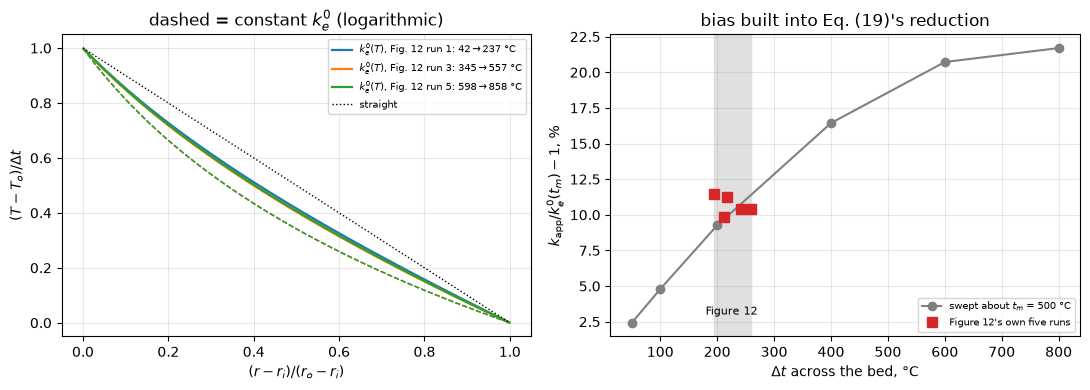
So the reading of the authors’ remark is asymmetric:
- Against a constant conductivity: strong. A constant-\(k_e^0\) annulus at this bore ratio departs from a straight line by the printed fraction of the temperature drop, at every \(\Delta t\). Figure 12’s profiles do not look like that, and no reading of the figure’s abscissa changes it.
- For Equation (15) specifically: partial. At the drops Figure 12 shows, Eq. (15) brings the departure down only by the printed factor, well short of the factor the swept minimum would suggest. Eq. (15)’s profile is still visibly bowed. Something makes the real bed straighter than Eq. (15) predicts, and this page does not know what.
Quoting the swept factor for this apparatus would be taking the best point of a sweep and attaching it to a condition the paper never ran.
Closing the assertion gap
recompute() runs before these last cells, so its first assertion covers only the numbers defined up to that point. The ones defined here are checked against it now, at the same tolerance. Without this cell a change to n=400 or to the sweep above would leave the break rows testing a different computation from the published one.
checked = {k: (METRICS[k], BASE[k]) for k in BASE}
bad = {k: v for k, v in checked.items() if not np.isclose(v[0], v[1], rtol=1e-8, atol=1e-12)}
worst = max(abs(a - b) / max(abs(b), 1e-300) for a, b in checked.values())
print(f"all {len(BASE)} metrics, narrative cells vs recompute(): worst relative difference "
      f"{worst:.2e}")
assert not bad, f"narrative cells disagree with recompute(): {bad}"
assert set(METRICS) == set(BASE), (
    f"reported but not in recompute(): {sorted(set(METRICS) - set(BASE))}; "
    f"in recompute() but never reported: {sorted(set(BASE) - set(METRICS))}")
print(f"recompute() and the narrative cells agree on all {len(BASE)} published metrics, and the "
      f"two sets are identical -- so no metric escapes the sweep and none is swept but unreported.")
all 94 metrics, narrative cells vs recompute(): worst relative difference 1.54e-12
recompute() and the narrative cells agree on all 94 published metrics, and the two sets are identical -- so no metric escapes the sweep and none is swept but unreported.The variable-conductivity solve: grid, and the second route
With \(k_e^0(T)\) the annulus is nonlinear. The page solves it with pymrm.newton on the scaled temperature, with a tridiagonal NumJac((n, 1)). The second route freezes the face conductivities, solves the linear problem and repeats (a fixed point), stopping when the largest change of a sweep is below tol degC. The cells below put the reported bias on a cell ladder, measure how fast the fixed point contracts, compare the two routes, and run the fixed point where its step stops falling.
RUN_LAST = f12.iloc[-1]                 # Figure 12's hottest run, a named data row


def bias_ladder(ns=(100, 200, 400, 800), n_pub=400, nu=1, kfun=None, row=RUN_LAST):
    """The reduction bias of one Figure 12 run on a ladder of cells (Newton solves)."""
    kfun = ke0_iron if kfun is None else kfun
    Ti, To = float(row.t_inside_C), float(row.t_outside_C)

    def bias(n):
        _, r_c, T, Qp = solve_annulus(n, Ti, To, kfun=kfun, nu=nu)
        vol = 2 * np.pi * r_c * (R_O - R_I) / n
        k_app = Qp[0] / (2 * np.pi) * np.log(R_O / R_I) / (Ti - To)
        return float(100 * (k_app / kfun(np.sum(vol * T) / vol.sum()) - 1))

    vals = {n: bias(n) for n in sorted(set(ns) | {n_pub})}
    study = observed_orders(lambda n: vals[n], ns)
    ops = annulus_operators(ns[-1], Ti, To, nu)
    cond = np.linalg.cond((ops["div"] @ ops["grad"]).toarray())
    return {"reduction_bias_order_min": float(np.min(study["orders"])),
            "reduction_bias_order_max": float(np.max(study["orders"])),
            "reduction_bias_grid_error_n400": float(abs(vals[n_pub] - study["extrapolated"])),
            "reduction_bias_roundoff_margin": float(abs(vals[ns[-1]] - vals[ns[-2]])
                                                    / (100 * cond * np.finfo(float).eps)),
            "_vals": vals, "_orders": study["orders"], "_extrapolated": study["extrapolated"]}


def picard_study(row=RUN_LAST, n=400, tol=1e-8, n_stall=1200, tol_stall=1e-10):
    """The fixed point against Newton on one Figure 12 run, and where its step stalls."""
    Ti, To = float(row.t_inside_C), float(row.t_outside_C)
    info_n, info_p = {}, {}
    _, _, Tn, _ = solve_annulus(n, Ti, To, kfun=ke0_iron, info=info_n)
    _, _, Tp, _ = solve_annulus(n, Ti, To, kfun=ke0_iron, method="picard", tol=tol, info=info_p)
    st = np.array(info_p["steps"])
    big = st[:-1] > 1e-6                 # sweeps well above the round-off floor
    stall = {}
    try:
        solve_annulus(n_stall, Ti, To, kfun=ke0_iron, method="picard", tol=tol_stall, info=stall)
    except RuntimeError:
        pass                             # reported through the steps it recorded
    info_c = {}
    _, _, Tc, _ = solve_annulus(n_stall, Ti, To, kfun=ke0_iron, method="picard", tol=tol, info=info_c)
    _, _, Tns, _ = solve_annulus(n_stall, Ti, To, kfun=ke0_iron, info=(newton_stall := {}))
    s2 = np.array(stall["steps"])
    big2 = s2[:-1] > 1e-6
    return {"picard_contraction_max": float(np.max(st[1:][big] / st[:-1][big])),
            "picard_n1200_contraction_max": float(np.max(s2[1:][big2] / s2[:-1][big2])),
            "picard_vs_newton_max_dT": float(np.max(np.abs(Tp - Tn)) / (Ti - To)),
            "picard_n1200_sweeps": float(len(info_c["steps"])),
            "picard_n1200_vs_newton_max_dT": float(np.max(np.abs(Tc - Tns)) / (Ti - To)),
            "picard_n1200_stall_step_C": float(np.median(stall["steps"][-100:])),
            "_sweeps": len(st), "_newton_it": info_n["iterations"],
            "_stall_sweeps": len(stall["steps"]), "_newton_stall_it": newton_stall["iterations"]}


STUDY = {}
BL = bias_ladder()
STUDY.update({k: v for k, v in BL.items() if not k.startswith("_")})
print(f"bias of the run {RUN_LAST.t_outside_C:.0f} -> {RUN_LAST.t_inside_C:.0f} degC on the ladder:")
for n, v in BL["_vals"].items():
    print(f"  n = {n:4d}: {v:.6f} %")
print(f"observed orders {', '.join(f'{o:.4f}' for o in BL['_orders'])}; Richardson limit "
      f"{BL['_extrapolated']:.6f} %; the 400-cell value is "
      f"{STUDY['reduction_bias_grid_error_n400']:.1e} percentage points from it")
print(f"finest difference over the round-off floor: {STUDY['reduction_bias_roundoff_margin']:.0f}")

PS = picard_study()
STUDY.update({k: v for k, v in PS.items() if not k.startswith("_")})
print(f"\nNewton: {PS['_newton_it']} iterations at 400 cells, {PS['_newton_stall_it']} at 1200.")
PICARD_TOL = 1e-8
print(f"fixed point at 400 cells: {PS['_sweeps']} sweeps to a {PICARD_TOL:g} degC step; each sweep shrinks "
      f"the step by a factor of at most {STUDY['picard_contraction_max']:.3f}")
print(f"the two routes agree to {STUDY['picard_vs_newton_max_dT']:.1e} of the temperature drop")
print(f"fixed point at 1200 cells: after {PS['_stall_sweeps']} sweeps the step fluctuates about "
      f"{STUDY['picard_n1200_stall_step_C']:.1e} degC (median of the last 100 sweeps), above the "
      f"1e-10 degC stopping rule it was given.")
print(f"with a {PICARD_TOL:g} degC rule the 1200-cell fixed point converges in "
      f"{STUDY['picard_n1200_sweeps']:.0f} sweeps, within {STUDY['picard_n1200_vs_newton_max_dT']:.1e} "
      f"of the temperature drop of Newton")
print(f"at 1200 cells each sweep above 1e-6 degC shrinks the step by at most "
      f"{STUDY['picard_n1200_contraction_max']:.3f}: the iteration contracts as fast as at 400 cells, "
      f"and stalls at {STUDY['picard_n1200_stall_step_C'] / float(RUN_LAST.t_inside_C):.0e} of the "
      f"hot-wall temperature, the round-off of the solve. Newton is unaffected.")
METRICS.update(STUDY)
bias of the run 598 -> 858 degC on the ladder:
n = 100: 10.408454 %
n = 200: 10.407205 %
n = 400: 10.406873 %
n = 800: 10.406788 %
observed orders 1.9094, 1.9680; Richardson limit 10.406759 %; the 400-cell value is 1.1e-04 percentage points from it
finest difference over the round-off floor: 12017
Newton: 4 iterations at 400 cells, 4 at 1200.
fixed point at 400 cells: 10 sweeps to a 1e-08 degC step; each sweep shrinks the step by a factor of at most 0.175
the two routes agree to 1.9e-12 of the temperature drop
fixed point at 1200 cells: after 300 sweeps the step fluctuates about 7.0e-10 degC (median of the last 100 sweeps), above the 1e-10 degC stopping rule it was given.
with a 1e-08 degC rule the 1200-cell fixed point converges in 10 sweeps, within 1.1e-12 of the temperature drop of Newton
at 1200 cells each sweep above 1e-6 degC shrinks the step by at most 0.174: the iteration contracts as fast as at 400 cells, and stalls at 8e-13 of the hot-wall temperature, the round-off of the solve. Newton is unaffected.Honestly, what is not added
Everything else on this page is reproduction or bookkeeping. The correlation is not improved, no constant is re-fitted, and no new data are brought to it. The model is algebra and pymrm is not needed to evaluate it, nu=1 earns its place only in the apparatus, which is where the two results above live.
Claims
Every number the page states, with how it is checked. Algebra on printed numbers and the solved bias and profile values are held to RTOL of the baseline; residuals, identities, orders and two-route gaps are bounds with their basis; counts carry the distance of the closest value to their threshold.
RTOL = 1e-6
BOUNDS = {
    "V1_identity_eq16_from_eq15": dict(max=1e-13, basis="identity",
                                       note="two printed forms of one equation, 20 000 draws"),
    "V3_eq13_from_network": dict(max=1e-13, basis="identity", note="Eq. (13) against its own network"),
    "delete_hrs_exact_reproduction_resid": dict(max=1e-13, basis="identity",
                                                note="phi inverted in closed form and put back"),
    "V2_eq14_limit_order": dict(min=0.99, max=1.01, basis="theory",
                                note="the kg -> 0 residual is O(kg): order 1"),
    "k_app_vs_closed_form_identity": dict(max=1e-5, basis="theory",
                                          note="400 cells, second order, against the T-average of ke0"),
    "V4_annulus_order_min": dict(min=1.9, max=2.05, basis="theory",
                                 note="second-order cells, ladder 100 to 800"),
    "V4_annulus_order_max": dict(min=1.9, max=2.05, basis="theory",
                                 note="second-order cells, ladder 100 to 800"),
    "V4_annulus_extrapolated_vs_closed_form": dict(max=1e-7, basis="theory",
                                                   note="Richardson limit; next-order terms"),
    "V4_annulus_roundoff_margin": dict(min=1e3, basis="theory",
                                       note="finest difference over cond(A) eps |Q|"),
    "V4_annulus_face_spread": dict(max=1e-10, basis="identity",
                                   note="the divergence telescopes; the gap is the solve's round-off"),
    "V4_annulus_profile_err_n800": dict(max=2e-7, basis="theory", note="second order on 800 cells"),
    "V4_pymrm_vs_closed_form": dict(max=1e-6, basis="theory", note="heat rate on 800 cells"),
    "annulus_varK_face_spread_max": dict(max=1e-10, basis="identity",
                                         note="energy balance of the converged Newton solve"),
    "reduction_bias_order_min": dict(min=1.85, max=2.05, basis="theory",
                                     note="second-order cells, 100 to 800"),
    "reduction_bias_order_max": dict(min=1.85, max=2.05, basis="theory",
                                     note="second-order cells, 100 to 800"),
    "reduction_bias_grid_error_n400": dict(max=1e-3, basis="chosen",
                                           note="percentage points; keeps the printed decimal"),
    "reduction_bias_roundoff_margin": dict(min=1e3, basis="theory",
                                           note="finest difference over 100 cond(A) eps, the round-off of the bias in per cent"),
    "radiation_share_fine_clinker_at_1200C_pct": dict(
        max=50.0, basis="theory",
        note="radiation share of ke0 at the end of the air table stays below half"),
    "picard_vs_newton_max_dT": dict(max=1e-11, basis="tolerance",
                                    note="fixed point stopped at a 1e-8 degC step, contraction <= 0.2"),
    "picard_n1200_vs_newton_max_dT": dict(max=1e-11, basis="tolerance",
                                          note="fixed point stopped at a 1e-8 degC step, contraction <= 0.2"),
    "picard_n1200_sweeps": dict(min=5, max=20, basis="tolerance",
                                note="sweeps to a 1e-8 degC step at 1200 cells"),
    "picard_n1200_stall_step_C": dict(min=1e-10, max=1e-7, basis="tolerance",
                                         note="median of the last 100 steps, above the 1e-10 degC stopping rule"),
}
cnt = {}
cnt["delete_hrs_rows_unmatched"] = claims.count(
    "delete_hrs_rows_unmatched", delete_results["h_rs"], 1e-9, min_margin=0.5,
    note="rows whose shortfall is positive; zero means matched")
cnt["delete_hrv_rows_unmatched"] = claims.count(
    "delete_hrv_rows_unmatched", delete_results["h_rv"], 1e-9, min_margin=0.5,
    note="rows whose shortfall is positive; zero means matched")
cnt["delete_gamma_rows_unmatched"] = claims.count(
    "delete_gamma_rows_unmatched", delete_results["gamma(kg/ks)"], 1e-9, min_margin=0.5,
    note="rows whose shortfall is positive; zero means matched")
cnt["delete_control_beta_half_rows_unmatched"] = claims.count(
    "delete_control_beta_half_rows_unmatched", delete_results["half the numerator"], 1e-9,
    min_margin=0.5, note="rows whose shortfall is positive; zero means matched")
_need = {k: v[np.isfinite(v)] for k, v in phi_needed_by.items()}
cnt["delete_hrs_rows_phi_above_printed"] = claims.count(
    "delete_hrs_rows_phi_above_printed", _need["h_rs"], PHI_PRINTED_HI, min_margin=0.02,
    note="phi needed above Table 4's largest printed phi")
cnt["delete_gamma_rows_phi_above_printed"] = claims.count(
    "delete_gamma_rows_phi_above_printed", _need["gamma(kg/ks)"], PHI_PRINTED_HI, min_margin=0.01,
    note="phi needed above Table 4's largest printed phi")
cnt["delete_gamma_rows_off_fig9_axis"] = claims.count(
    "delete_gamma_rows_off_fig9_axis", _need["gamma(kg/ks)"], PHI_FIG9_TOP, min_margin=0.02,
    note="phi needed above the top of Figure 9's ordinate")
cnt["fig13to17_curve_ends_positive_count"] = claims.count(
    "fig13to17_curve_ends_positive_count", d10, 0.0, min_margin=0.1,
    note="curve ends that Eq. (15) at p = 1 overshoots; margin in per cent")
cnt["fig13to17_within_reading_error_p10"] = claims.count(
    "fig13to17_within_reading_error_p10", np.abs(d10) - READ_ERR_PCT, 0.0, above=False,
    min_margin=0.01, note="|deviation| inside the sidecar's reading error; margin in per cent")
cnt["fig13to17_within_reading_error_p09"] = claims.count(
    "fig13to17_within_reading_error_p09", np.abs(d09) - READ_ERR_PCT, 0.0, above=False,
    min_margin=0.01, note="|deviation| inside the sidecar's reading error; margin in per cent")
for k, v in cnt.items():
    assert v == METRICS[k], (k, v, METRICS[k])
_nz = cross.dev_pct.abs()[cross.dev_pct.abs() >= 1e-12]
claims.exact("table1_vs_table3_identical_rows", int(METRICS["table1_vs_table3_identical_rows"]),
             margin=float(_nz.min()), min_margin=0.01,
             note="shared references whose two printed values are identical; margin the smallest "
                  "nonzero |deviation| in per cent")
claims.exact("table1_vs_table3_daggered_rows", int(METRICS["table1_vs_table3_daggered_rows"]),
             note="shared references Table 3 daggers as extrapolated to zero flow")
claims.exact("alpha_beta_ordinary_in_printed_band_frac",
             float(METRICS["alpha_beta_ordinary_in_printed_band_frac"]),
             note="share of the printed alpha-beta values of ordinary packings inside the printed "
                  "0.1 to 0.14, compared as printed")
for k, kw in BOUNDS.items():
    claims.bound(k, METRICS[k], **kw)
for k, v in METRICS.items():
    if k not in claims.metrics:
        claims.value(k, v, rtol=RTOL)
assert set(claims.metrics) == set(METRICS)
print(f"{len(claims.metrics)} claims registered")
104 claims registeredThe defect-injection table
Every claim needs a row that fails its own check. The rows of INJECTIONS each rerun the whole of recompute() with one defect, so every claim a defect reaches is tested. The ladder, the fixed point and the round-off claims get rows of their own, each a call argument of their study. A quantity that cannot be computed under a defect (a crossing the scan no longer finds) records nan, which fails its claim.
BREAK = []


def brk(row, name, broken):
    """One injected defect: ``broken`` is what claim ``name`` becomes with it."""
    if isinstance(broken, (float, np.floating)) and not np.isfinite(broken):
        broken = np.nan
    BREAK.append((row, name, claims.breaks(row, name, broken)))


def study_row(label, result):
    for name, v in result.items():
        if name in claims.metrics:
            brk(label, name, v)


for label, B in BROKEN.items():
    study_row(label, B)
_flat = lambda T: 1.0 + 0.0 * np.asarray(T, float)
study_row("annulus ladder started at 4 cells", annulus_study(c_two_pi_ln, ns=(4, 8, 16, 32)))
study_row("bias ladder started at 4 cells", bias_ladder(ns=(4, 8, 16, 32)))
study_row("bias published from 50 cells", bias_ladder(n_pub=50))
study_row("Cartesian bed with a constant k, where the scheme is exact",
          bias_ladder(nu=0, kfun=_flat))
study_row("fixed point stopped at a 1e-3 degC step", picard_study(tol=1e-3))
study_row("fixed point run on the swept 800 degC drop",
          picard_study(row=pd.Series(dict(t_inside_C=900.0, t_outside_C=100.0))))
study_row("fixed point stall measured at 400 cells", picard_study(n_stall=400))

bt = pd.DataFrame(BREAK, columns=["row", "claim", "caught"])
caught = bt[bt.caught].groupby("row", sort=False).claim.apply(list)
print(f"{len(bt.row.unique())} rows; claims each row fails:")
for row, names in caught.items():
    print(f"  {row}:")
    print("      " + ", ".join(names))
idle = [r for r in bt.row.unique() if r not in caught.index]
print(f"\nrows that fail no claim: {idle if idle else 'none'}")
missing = [n for n in claims.metrics
           if not claims.metrics[n].get("structural") and not bt[(bt.claim == n) & bt.caught].shape[0]]
print(f"claims no row fails: {missing if missing else 'none'}")
34 rows; claims each row fails:
Eq. (17) numerator pi l, exactly as printed:
eq19_constant_2pi_vs_printed_pct, eq19_constant_exact_ln_vs_printed_pct, V4_pymrm_vs_closed_form
D_i read as 0.0357 instead of 0.0375:
eq17_as_printed_over_eq19_ratio, eq19_constant_2pi_vs_printed_pct, eq19_constant_exact_ln_vs_printed_pct, V4_pymrm_vs_closed_form
kg frozen at its 0 degC value, not the printed kg(t):
table4_ks_over_kg_roundtrip_pct, phi_implied_spread_at_eps040, phi_implied_spread_at_eps040_no_celite, phi_implied_median_at_eps040, forward_from_phi_line_vs_calcd_mean_abs_pct, forward_from_phi_line_vs_exp_mean_abs_pct, table3_max_void_radiation_share_pct, table3_max_hrs_share_of_contact_pct, delete_hrs_max_phi_needed, delete_hrs_rows_phi_above_printed, delete_hrv_rows_unmatched, delete_hrv_worst_shortfall_pct, delete_gamma_rows_unmatched, delete_gamma_max_phi_needed, delete_gamma_rows_phi_above_printed, delete_control_beta_half_rows_unmatched, delete_control_beta_half_worst_shortfall_pct, delete_hrs_max_phi_shift_pct, radiation_half_temp_iron_sphere_C, radiation_half_temp_firebrick_sphere_C, fine_clinker_spread_pct_200_1000C, coarse_clinker_spread_pct_200_1000C, iron_sphere_spread_pct_200_1000C, raschig_random_over_regular_at_600C, raschig_random_over_regular_min_pct, raschig_random_over_regular_max_pct, gamma_printed_decimal_cost_at_400C_pct, V5_emissivity_p08_vs_p10_at_1000C_pct, V5_emissivity_p06_vs_p10_at_1000C_pct, fig13to17_curve_ends_mean_abs_pct, fig13to17_curve_ends_worst_abs_pct, fig13to17_curve_ends_mean_abs_pct_at_p08, fig13to17_curve_ends_se_pct, fig13to17_within_reading_error_p10, fig13to17_within_reading_error_p09, fig13to17_mean_dev_pct_at_p09, fig13to17_mean_dev_pct_at_p08, fig13to17_p_zero_mean_dev, fig13to17_p_zero_offset_lo, fig13to17_p_zero_offset_hi, firebrick_curve_ends_mean_abs_pct_ks_const, firebrick_curve_ends_mean_abs_pct_ratio_const, radiation_half_temp_firebrick_sphere_C_ks_over_kg_const, reduction_bias_swept_min_pct, reduction_bias_swept_max_pct, nonstraightness_varK_swept_min, reduction_bias_min_pct, reduction_bias_max_pct, nonstraightness_varK_at_fig12_max, straightness_factor_at_fig12_min
0.1952 in Eqs. (7)-(8) read as 0.01952:
phi_implied_spread_at_eps040, phi_implied_spread_at_eps040_no_celite, phi_implied_median_at_eps040, forward_from_phi_line_vs_calcd_mean_abs_pct, forward_from_phi_line_vs_exp_mean_abs_pct, table3_max_void_radiation_share_pct, table3_max_hrs_share_of_contact_pct, delete_hrs_rows_unmatched, delete_hrs_max_phi_needed, delete_hrv_worst_shortfall_pct, delete_gamma_max_phi_needed, delete_gamma_rows_phi_above_printed, delete_gamma_rows_off_fig9_axis, delete_control_beta_half_worst_shortfall_pct, delete_hrs_exact_reproduction_resid, delete_hrs_max_phi_shift_pct, radiation_half_temp_iron_sphere_C, radiation_half_temp_firebrick_sphere_C, fine_clinker_spread_pct_200_1000C, coarse_clinker_spread_pct_200_1000C, iron_sphere_spread_pct_200_1000C, raschig_random_over_regular_at_600C, raschig_random_over_regular_min_pct, raschig_random_over_regular_max_pct, gamma_printed_decimal_cost_at_400C_pct, V5_emissivity_p08_vs_p10_at_1000C_pct, V5_emissivity_p06_vs_p10_at_1000C_pct, fig13to17_curve_ends_mean_abs_pct, fig13to17_curve_ends_worst_abs_pct, fig13to17_curve_ends_mean_abs_pct_at_p08, fig13to17_curve_ends_se_pct, fig13to17_curve_ends_positive_count, fig13to17_within_reading_error_p10, fig13to17_within_reading_error_p09, fig13to17_mean_dev_pct_at_p09, fig13to17_mean_dev_pct_at_p08, fig13to17_p_zero_mean_dev, fig13to17_p_zero_offset_lo, fig13to17_p_zero_offset_hi, firebrick_curve_ends_mean_abs_pct_ks_const, firebrick_curve_ends_mean_abs_pct_ratio_const, radiation_half_temp_firebrick_sphere_C_ks_over_kg_const, reduction_bias_swept_min_pct, reduction_bias_swept_max_pct, nonstraightness_varK_swept_min, reduction_bias_min_pct, reduction_bias_max_pct, nonstraightness_varK_at_fig12_max, straightness_factor_at_fig12_min
emissivity p = 0.8 instead of the assumed 1.0:
phi_implied_spread_at_eps040, phi_implied_spread_at_eps040_no_celite, phi_implied_median_at_eps040, forward_from_phi_line_vs_calcd_mean_abs_pct, forward_from_phi_line_vs_exp_mean_abs_pct, table3_max_void_radiation_share_pct, table3_max_hrs_share_of_contact_pct, delete_hrs_max_phi_needed, delete_gamma_max_phi_needed, delete_gamma_rows_phi_above_printed, delete_control_beta_half_worst_shortfall_pct, delete_hrs_max_phi_shift_pct, radiation_half_temp_iron_sphere_C, radiation_half_temp_firebrick_sphere_C, fine_clinker_spread_pct_200_1000C, coarse_clinker_spread_pct_200_1000C, iron_sphere_spread_pct_200_1000C, raschig_random_over_regular_at_600C, raschig_random_over_regular_min_pct, raschig_random_over_regular_max_pct, gamma_printed_decimal_cost_at_400C_pct, V5_emissivity_p08_vs_p10_at_1000C_pct, V5_emissivity_p06_vs_p10_at_1000C_pct, fig13to17_curve_ends_mean_abs_pct, fig13to17_curve_ends_worst_abs_pct, fig13to17_curve_ends_se_pct, fig13to17_curve_ends_positive_count, firebrick_curve_ends_mean_abs_pct_ks_const, firebrick_curve_ends_mean_abs_pct_ratio_const, radiation_half_temp_firebrick_sphere_C_ks_over_kg_const, reduction_bias_swept_min_pct, reduction_bias_swept_max_pct, nonstraightness_varK_swept_min, reduction_bias_min_pct, reduction_bias_max_pct, nonstraightness_varK_at_fig12_max, straightness_factor_at_fig12_min
rings given the ordinary gamma = 1:
raschig_random_over_regular_at_600C, raschig_random_over_regular_min_pct, raschig_random_over_regular_max_pct, gamma_printed_decimal_cost_at_400C_pct
random-packing beta set to the regular 1/sqrt(3):
raschig_random_over_regular_at_600C, raschig_random_over_regular_min_pct, raschig_random_over_regular_max_pct
the 0.35~0.01 mm row read as firebrick, ks 1.7 -> 0.20:
fine_clinker_spread_pct_200_1000C
deviation taken as measured/model (reciprocal):
paper_calcd_vs_exp_mean_abs_pct, paper_calcd_vs_exp_bias_pct, paper_calcd_vs_exp_worst_abs_pct, paper_calcd_vs_exp_mean_abs_pct_no_celite, paper_calcd_vs_exp_bias_se_pct
rings and saddles left in the ordinary alpha-beta group:
alpha_beta_ordinary_mean, alpha_beta_ordinary_in_printed_band_frac, alpha_beta_ring_over_ordinary_ratio, alpha_beta_theory_over_observed_lower
Table 3's Exp column shifted by one row:
paper_calcd_vs_exp_mean_abs_pct, paper_calcd_vs_exp_bias_pct, paper_calcd_vs_exp_worst_abs_pct, paper_calcd_vs_exp_mean_abs_pct_no_celite, paper_calcd_vs_exp_bias_se_pct, table1_vs_table3_exp_max_abs_pct, table1_vs_table3_identical_rows, table1_vs_table3_daggered_rows
Table 1's ke0/kg intercept column shifted by one row:
static_dynamic_crossover_PeM_median, table1_vs_table3_exp_max_abs_pct, table1_vs_table3_identical_rows, table1_vs_table3_daggered_rows
construct_div(nu=1) -> nu=0 (Cartesian):
V4_annulus_order_min, V4_annulus_order_max, V4_annulus_extrapolated_vs_closed_form, V4_annulus_roundoff_margin, V4_annulus_face_spread, V4_annulus_profile_err_n800, V4_pymrm_constant_vs_printed_pct, V4_pymrm_vs_closed_form, reduction_bias_swept_min_pct, reduction_bias_swept_max_pct, k_app_vs_closed_form_identity, tm_fraction_of_dT_constant_k, nonstraightness_constant_k, nonstraightness_varK_swept_min, reduction_bias_min_pct, reduction_bias_max_pct, nonstraightness_varK_at_fig12_max, straightness_factor_at_fig12_min, annulus_varK_face_spread_max
sign flip on the contact term in Eq. (15):
forward_from_phi_line_vs_calcd_mean_abs_pct, forward_from_phi_line_vs_exp_mean_abs_pct, delete_hrs_max_phi_needed, delete_hrs_rows_phi_above_printed, delete_hrv_worst_shortfall_pct, delete_gamma_rows_unmatched, delete_gamma_max_phi_needed, delete_gamma_rows_phi_above_printed, delete_gamma_rows_off_fig9_axis, delete_control_beta_half_worst_shortfall_pct, delete_hrs_exact_reproduction_resid, radiation_half_temp_iron_sphere_C, radiation_half_temp_firebrick_sphere_C, fine_clinker_spread_pct_200_1000C, coarse_clinker_spread_pct_200_1000C, iron_sphere_spread_pct_200_1000C, raschig_random_over_regular_at_600C, raschig_random_over_regular_min_pct, raschig_random_over_regular_max_pct, gamma_printed_decimal_cost_at_400C_pct, V5_emissivity_p08_vs_p10_at_1000C_pct, V5_emissivity_p06_vs_p10_at_1000C_pct, fig13to17_curve_ends_mean_abs_pct, fig13to17_curve_ends_worst_abs_pct, fig13to17_curve_ends_mean_abs_pct_at_p08, fig13to17_curve_ends_se_pct, fig13to17_curve_ends_positive_count, fig13to17_within_reading_error_p10, fig13to17_within_reading_error_p09, fig13to17_mean_dev_pct_at_p09, fig13to17_mean_dev_pct_at_p08, fig13to17_p_zero_mean_dev, fig13to17_p_zero_offset_lo, fig13to17_p_zero_offset_hi, firebrick_curve_ends_mean_abs_pct_ks_const, firebrick_curve_ends_mean_abs_pct_ratio_const, radiation_half_temp_firebrick_sphere_C_ks_over_kg_const, V1_identity_eq16_from_eq15, V2_eq14_limit_order, V2_eq14_residual_at_1e-7, reduction_bias_swept_min_pct, reduction_bias_swept_max_pct, nonstraightness_varK_swept_min, reduction_bias_min_pct, reduction_bias_max_pct, nonstraightness_varK_at_fig12_max, straightness_factor_at_fig12_min
1/phi in Eq. (15) read as phi:
forward_from_phi_line_vs_calcd_mean_abs_pct, forward_from_phi_line_vs_exp_mean_abs_pct, delete_hrs_rows_unmatched, delete_hrs_max_phi_needed, delete_hrv_rows_unmatched, delete_hrv_worst_shortfall_pct, delete_gamma_rows_unmatched, delete_gamma_max_phi_needed, delete_gamma_rows_phi_above_printed, delete_gamma_rows_off_fig9_axis, delete_control_beta_half_rows_unmatched, delete_control_beta_half_worst_shortfall_pct, delete_hrs_exact_reproduction_resid, radiation_half_temp_iron_sphere_C, radiation_half_temp_firebrick_sphere_C, radiation_share_fine_clinker_at_1200C_pct, fine_clinker_spread_pct_200_1000C, coarse_clinker_spread_pct_200_1000C, iron_sphere_spread_pct_200_1000C, raschig_random_over_regular_at_600C, raschig_random_over_regular_min_pct, raschig_random_over_regular_max_pct, gamma_printed_decimal_cost_at_400C_pct, V5_emissivity_p08_vs_p10_at_1000C_pct, V5_emissivity_p06_vs_p10_at_1000C_pct, fig13to17_curve_ends_mean_abs_pct, fig13to17_curve_ends_worst_abs_pct, fig13to17_curve_ends_mean_abs_pct_at_p08, fig13to17_curve_ends_se_pct, fig13to17_curve_ends_positive_count, fig13to17_within_reading_error_p10, fig13to17_within_reading_error_p09, fig13to17_mean_dev_pct_at_p09, fig13to17_mean_dev_pct_at_p08, fig13to17_p_zero_mean_dev, fig13to17_p_zero_offset_lo, fig13to17_p_zero_offset_hi, firebrick_curve_ends_mean_abs_pct_ks_const, firebrick_curve_ends_mean_abs_pct_ratio_const, radiation_half_temp_firebrick_sphere_C_ks_over_kg_const, V1_identity_eq16_from_eq15, V2_eq14_residual_at_1e-7, reduction_bias_swept_min_pct, reduction_bias_swept_max_pct, nonstraightness_varK_swept_min, reduction_bias_min_pct, reduction_bias_max_pct, nonstraightness_varK_at_fig12_max, straightness_factor_at_fig12_min
gamma(kg/ks) dropped from Eq. (15)'s denominator:
forward_from_phi_line_vs_calcd_mean_abs_pct, forward_from_phi_line_vs_exp_mean_abs_pct, delete_hrs_max_phi_needed, delete_hrs_rows_phi_above_printed, delete_hrv_rows_unmatched, delete_hrv_worst_shortfall_pct, delete_control_beta_half_rows_unmatched, delete_control_beta_half_worst_shortfall_pct, delete_hrs_exact_reproduction_resid, radiation_half_temp_iron_sphere_C, radiation_half_temp_firebrick_sphere_C, fine_clinker_spread_pct_200_1000C, coarse_clinker_spread_pct_200_1000C, iron_sphere_spread_pct_200_1000C, raschig_random_over_regular_at_600C, raschig_random_over_regular_min_pct, raschig_random_over_regular_max_pct, gamma_printed_decimal_cost_at_400C_pct, V5_emissivity_p08_vs_p10_at_1000C_pct, V5_emissivity_p06_vs_p10_at_1000C_pct, fig13to17_curve_ends_mean_abs_pct, fig13to17_curve_ends_worst_abs_pct, fig13to17_curve_ends_mean_abs_pct_at_p08, fig13to17_curve_ends_se_pct, fig13to17_within_reading_error_p10, fig13to17_within_reading_error_p09, fig13to17_mean_dev_pct_at_p09, fig13to17_mean_dev_pct_at_p08, fig13to17_p_zero_mean_dev, fig13to17_p_zero_offset_lo, fig13to17_p_zero_offset_hi, firebrick_curve_ends_mean_abs_pct_ks_const, firebrick_curve_ends_mean_abs_pct_ratio_const, radiation_half_temp_firebrick_sphere_C_ks_over_kg_const, V1_identity_eq16_from_eq15, V2_eq14_limit_order, V2_eq14_residual_at_1e-7, reduction_bias_swept_min_pct, reduction_bias_swept_max_pct, nonstraightness_varK_swept_min, reduction_bias_min_pct, reduction_bias_max_pct, nonstraightness_varK_at_fig12_max, straightness_factor_at_fig12_min
N = 1/Dp instead of Ranz's 1/(beta Dp):
V3_eq13_from_network
the eps = 0.54 pair dropped from the phi(eps) fit:
phi_line_at_eps040_vs_printed_0034_pct, forward_from_phi_line_vs_calcd_mean_abs_pct, forward_from_phi_line_vs_exp_mean_abs_pct
beta = 1 taken as 0.85 throughout the phi inversion:
forward_from_phi_line_vs_calcd_mean_abs_pct, forward_from_phi_line_vs_exp_mean_abs_pct, delete_hrs_rows_unmatched, delete_hrs_max_phi_needed, delete_hrv_rows_unmatched, delete_hrv_worst_shortfall_pct, delete_gamma_max_phi_needed, delete_gamma_rows_phi_above_printed, delete_control_beta_half_rows_unmatched, delete_control_beta_half_worst_shortfall_pct, delete_hrs_exact_reproduction_resid
gamma = 1 taken as 0.5 throughout the phi inversion:
phi_implied_spread_at_eps040, phi_implied_spread_at_eps040_no_celite, phi_implied_median_at_eps040, forward_from_phi_line_vs_calcd_mean_abs_pct, forward_from_phi_line_vs_exp_mean_abs_pct, table3_max_hrs_share_of_contact_pct, delete_hrs_max_phi_needed, delete_hrs_rows_phi_above_printed, delete_hrv_rows_unmatched, delete_hrv_worst_shortfall_pct, delete_control_beta_half_rows_unmatched, delete_control_beta_half_worst_shortfall_pct, delete_hrs_max_phi_shift_pct
Eqs. (7) and (8) EXCHANGED wholesale:
V5_emissivity_p08_vs_p10_at_1000C_pct, V5_emissivity_p06_vs_p10_at_1000C_pct, V5_hrs_over_hrv_at_p06_eps040, V5_hrs_p06_over_blackbody, V5_hrv_eps_spread_at_p06_pct, fig13to17_curve_ends_mean_abs_pct_at_p08, fig13to17_within_reading_error_p09, fig13to17_mean_dev_pct_at_p09, fig13to17_mean_dev_pct_at_p08, fig13to17_p_zero_mean_dev, fig13to17_p_zero_offset_lo, fig13to17_p_zero_offset_hi
Eq. (7)'s p-group read as 2p/(1+p):
V5_emissivity_p08_vs_p10_at_1000C_pct, V5_emissivity_p06_vs_p10_at_1000C_pct, V5_hrs_over_hrv_at_p06_eps040, V5_hrs_p06_over_blackbody, fig13to17_curve_ends_mean_abs_pct_at_p08, fig13to17_mean_dev_pct_at_p09, fig13to17_mean_dev_pct_at_p08, fig13to17_p_zero_mean_dev, fig13to17_p_zero_offset_lo, fig13to17_p_zero_offset_hi
Eq. (8)'s eps-group inverted to (1-eps)/2eps:
V5_emissivity_p08_vs_p10_at_1000C_pct, V5_emissivity_p06_vs_p10_at_1000C_pct, V5_hrs_over_hrv_at_p06_eps040, V5_hrv_eps_spread_at_p06_pct, fig13to17_curve_ends_mean_abs_pct_at_p08, fig13to17_within_reading_error_p09, fig13to17_mean_dev_pct_at_p09, fig13to17_mean_dev_pct_at_p08, fig13to17_p_zero_mean_dev, fig13to17_p_zero_offset_lo, fig13to17_p_zero_offset_hi
reference 15 paired to Table 1 by row order, not packing:
table1_vs_table3_exp_max_abs_pct, table1_vs_table3_identical_rows
Figure 12's endpoints each read 3 degC out (its stated error):
fig12_dT_min_C, fig12_dT_max_C, reduction_bias_min_pct, reduction_bias_max_pct, nonstraightness_varK_at_fig12_max, straightness_factor_at_fig12_min
annulus fixed point stopped at a 0.1 degC step:
reduction_bias_swept_min_pct, reduction_bias_swept_max_pct, k_app_vs_closed_form_identity, nonstraightness_varK_swept_min, reduction_bias_min_pct, reduction_bias_max_pct, nonstraightness_varK_at_fig12_max, straightness_factor_at_fig12_min, annulus_varK_face_spread_max
curve-end reading error +-0.15 read as +-0.015:
fig13to17_reading_error_mean_pct, fig13to17_within_reading_error_p10, fig13to17_within_reading_error_p09, fig13to17_p_zero_offset_lo, fig13to17_p_zero_offset_hi
annulus ladder started at 4 cells:
V4_annulus_order_min, V4_annulus_order_max, V4_annulus_extrapolated_vs_closed_form
bias ladder started at 4 cells:
reduction_bias_order_min, reduction_bias_order_max, reduction_bias_grid_error_n400
bias published from 50 cells:
reduction_bias_grid_error_n400
Cartesian bed with a constant k, where the scheme is exact:
reduction_bias_order_min, reduction_bias_order_max, reduction_bias_roundoff_margin
fixed point stopped at a 1e-3 degC step:
picard_contraction_max, picard_vs_newton_max_dT, picard_n1200_vs_newton_max_dT
fixed point run on the swept 800 degC drop:
picard_contraction_max, picard_n1200_contraction_max, picard_n1200_sweeps
fixed point stall measured at 400 cells:
picard_n1200_contraction_max, picard_n1200_stall_step_C
rows that fail no claim: none
claims no row fails: none# Claims: prints every registered number, writes agreement.json for CI, and
# raises if any check failed or any claim has no break row.
claims.report(); # the semicolon keeps the notebook from echoing the payloadClaims for A3.12:
delete_hrs_rows_unmatched = 0 exact exact, margin 1
delete_hrv_rows_unmatched = 2 exact exact, margin 1
delete_gamma_rows_unmatched = 0 exact exact, margin 1
delete_control_beta_half_rows_unmatched = 6 exact exact, margin 1
delete_hrs_rows_phi_above_printed = 0 exact exact, margin 0.0972
delete_gamma_rows_phi_above_printed = 12 exact exact, margin 0.0178
delete_gamma_rows_off_fig9_axis = 2 exact exact, margin 0.109
fig13to17_curve_ends_positive_count = 14 exact exact, margin 0.562
fig13to17_within_reading_error_p10 = 4 exact exact, margin 0.24
fig13to17_within_reading_error_p09 = 9 exact exact, margin 0.145
table1_vs_table3_identical_rows = 3 exact exact, margin 6.14
table1_vs_table3_daggered_rows = 5 exact exact
alpha_beta_ordinary_in_printed_band_frac = 0.84615 exact exact
V1_identity_eq16_from_eq15 = (here 4.4e-16) bound bound <= 1e-13 [identity]
V3_eq13_from_network = (here 8.9e-16) bound bound <= 1e-13 [identity]
delete_hrs_exact_reproduction_resid = (here 2.2e-16) bound bound <= 1e-13 [identity]
V2_eq14_limit_order = (here 1.0e+00) bound bound [0.99, 1.01] [theory]
k_app_vs_closed_form_identity = (here 1.5e-06) bound bound <= 1e-05 [theory]
V4_annulus_order_min = (here 1.9e+00) bound bound [1.9, 2.05] [theory]
V4_annulus_order_max = (here 2.0e+00) bound bound [1.9, 2.05] [theory]
V4_annulus_extrapolated_vs_closed_form = (here 8.1e-09) bound bound <= 1e-07 [theory]
V4_annulus_roundoff_margin = (here 1.5e+04) bound bound >= 1000 [theory]
V4_annulus_face_spread = (here 4.0e-12) bound bound <= 1e-10 [identity]
V4_annulus_profile_err_n800 = (here 1.1e-07) bound bound <= 2e-07 [theory]
V4_pymrm_vs_closed_form = (here 3.7e-07) bound bound <= 1e-06 [theory]
annulus_varK_face_spread_max = (here 1.3e-12) bound bound <= 1e-10 [identity]
reduction_bias_order_min = (here 1.9e+00) bound bound [1.85, 2.05] [theory]
reduction_bias_order_max = (here 2.0e+00) bound bound [1.85, 2.05] [theory]
reduction_bias_grid_error_n400 = (here 1.1e-04) bound bound <= 0.001 [chosen]
reduction_bias_roundoff_margin = (here 1.2e+04) bound bound >= 1000 [theory]
radiation_share_fine_clinker_at_1200C_pct = (here 2.0e+01) bound bound <= 50 [theory]
picard_vs_newton_max_dT = (here 1.9e-12) bound bound <= 1e-11 [tolerance]
picard_n1200_vs_newton_max_dT = (here 1.1e-12) bound bound <= 1e-11 [tolerance]
picard_n1200_sweeps = (here 1.0e+01) bound bound [5, 20] [tolerance]
picard_n1200_stall_step_C = (here 7.0e-10) bound bound [1e-10, 1e-07] [tolerance]
eq17_as_printed_over_eq19_ratio = 2.001 value rtol 1e-06
eq19_constant_2pi_vs_printed_pct = 0.047505 value rtol 1e-06
eq19_constant_exact_ln_vs_printed_pct = 0.15995 value rtol 1e-06
table4_ks_over_kg_roundtrip_pct = -0.12784 value rtol 1e-06
alpha_beta_ordinary_mean = 0.1101 value rtol 1e-06
alpha_beta_ring_over_ordinary_ratio = 1.7166 value rtol 1e-06
alpha_beta_theory_over_observed_lower = 1.3332 value rtol 1e-06
static_dynamic_crossover_PeM_median = 50.5 value rtol 1e-06
table1_vs_table3_exp_max_abs_pct = 8.7719 value rtol 1e-06
paper_calcd_vs_exp_mean_abs_pct = 15.32 value rtol 1e-06
paper_calcd_vs_exp_bias_pct = -3.4592 value rtol 1e-06
paper_calcd_vs_exp_worst_abs_pct = 52 value rtol 1e-06
paper_calcd_vs_exp_mean_abs_pct_no_celite = 13.042 value rtol 1e-06
paper_calcd_vs_exp_bias_se_pct = 5.5441 value rtol 1e-06
phi_implied_spread_at_eps040 = 7.5557 value rtol 1e-06
phi_implied_spread_at_eps040_no_celite = 2.3012 value rtol 1e-06
phi_implied_median_at_eps040 = 0.031799 value rtol 1e-06
phi_line_at_eps040_vs_printed_0034_pct = 1.7337 value rtol 1e-06
forward_from_phi_line_vs_calcd_mean_abs_pct = 10.632 value rtol 1e-06
forward_from_phi_line_vs_exp_mean_abs_pct = 20.947 value rtol 1e-06
table3_max_void_radiation_share_pct = 30.466 value rtol 1e-06
table3_max_hrs_share_of_contact_pct = 29.714 value rtol 1e-06
delete_hrs_max_phi_shift_pct = 29.714 value rtol 1e-06
delete_hrs_max_phi_needed = 0.054169 value rtol 1e-06
delete_hrv_worst_shortfall_pct = 14.155 value rtol 1e-06
delete_gamma_max_phi_needed = 0.41954 value rtol 1e-06
delete_control_beta_half_worst_shortfall_pct = 46.664 value rtol 1e-06
radiation_half_temp_iron_sphere_C = 461.08 value rtol 1e-06
radiation_half_temp_firebrick_sphere_C = 264.91 value rtol 1e-06
fine_clinker_spread_pct_200_1000C = 9.5378 value rtol 1e-06
coarse_clinker_spread_pct_200_1000C = 153.97 value rtol 1e-06
iron_sphere_spread_pct_200_1000C = 228.06 value rtol 1e-06
raschig_random_over_regular_at_600C = 1.2024 value rtol 1e-06
raschig_random_over_regular_min_pct = 12.936 value rtol 1e-06
raschig_random_over_regular_max_pct = 24.39 value rtol 1e-06
gamma_printed_decimal_cost_at_400C_pct = 9.2092 value rtol 1e-06
fig13to17_curve_ends_mean_abs_pct = 2.4396 value rtol 1e-06
fig13to17_curve_ends_worst_abs_pct = 4.2447 value rtol 1e-06
fig13to17_curve_ends_mean_abs_pct_at_p08 = 5.0183 value rtol 1e-06
fig13to17_reading_error_mean_pct = 1.2974 value rtol 1e-06
fig13to17_curve_ends_se_pct = 0.35307 value rtol 1e-06
fig13to17_mean_dev_pct_at_p09 = -1.282 value rtol 1e-06
fig13to17_mean_dev_pct_at_p08 = -4.9162 value rtol 1e-06
fig13to17_p_zero_mean_dev = 0.93479 value rtol 1e-06
fig13to17_p_zero_offset_lo = 0.89907 value rtol 1e-06
fig13to17_p_zero_offset_hi = 0.96955 value rtol 1e-06
firebrick_curve_ends_mean_abs_pct_ks_const = 37.224 value rtol 1e-06
firebrick_curve_ends_mean_abs_pct_ratio_const = 3.5263 value rtol 1e-06
radiation_half_temp_firebrick_sphere_C_ks_over_kg_const = 233.27 value rtol 1e-06
V2_eq14_residual_at_1e-7 = 0.00015933 value rtol 1e-06
V4_pymrm_constant_vs_printed_pct = 0.15992 value rtol 1e-06
V5_emissivity_p08_vs_p10_at_1000C_pct = -16.361 value rtol 1e-06
V5_hrs_over_hrv_at_p06_eps040 = 0.52381 value rtol 1e-06
V5_hrs_p06_over_blackbody = 0.42857 value rtol 1e-06
V5_hrv_eps_spread_at_p06_pct = 16.667 value rtol 1e-06
V5_emissivity_p06_vs_p10_at_1000C_pct = -30.286 value rtol 1e-06
reduction_bias_swept_min_pct = 2.4256 value rtol 1e-06
reduction_bias_swept_max_pct = 21.699 value rtol 1e-06
tm_fraction_of_dT_constant_k = 0.70279 value rtol 1e-06
nonstraightness_constant_k = 0.13733 value rtol 1e-06
nonstraightness_varK_swept_min = 0.030233 value rtol 1e-06
fig12_dT_min_C = 195 value rtol 1e-06
fig12_dT_max_C = 260 value rtol 1e-06
reduction_bias_min_pct = 9.8348 value rtol 1e-06
reduction_bias_max_pct = 11.462 value rtol 1e-06
nonstraightness_varK_at_fig12_max = 0.082591 value rtol 1e-06
straightness_factor_at_fig12_min = 1.6628 value rtol 1e-06
picard_contraction_max = 0.17525 value rtol 1e-06
picard_n1200_contraction_max = 0.17373 value rtol 1e-06Reuse
Use Equation (15) when you need a stagnant-bed conductivity and you know \(\epsilon\), \(D_p\), \(k_s\), \(k_g\) and can defend a value for \(\varphi\). It is additive, cheap, and its temperature dependence is physically motivated rather than fitted.
Before you trust the radiation terms, know what is behind them. On the only table of numbers in the paper, the solid-to-solid coefficient \(h_{rs}\) is degenerate with \(\varphi\) and can be deleted without changing a single reproduced value, and the \(\varphi\) that absorbs it never leaves Table 4’s own printed band, so the degeneracy is real and not an artefact of a wide search. The void-to-void coefficient \(h_{rv}\) resists deletion on 2 rows of 14. \(\gamma\), by contrast, is identifiable: deleting it demands \(\varphi\) up to 0.42, twelve of the fourteen rows above every printed value and two off the top of Figure 9’s axis. The evidence for the radiation mechanism is in Figures 13–17, a temperature sweep on one packing at a time, which is exactly what separates a \(T^3\) term from a constant geometric ratio, and this page does not read them. Treat the radiation terms as supported by evidence this page has not examined, not as validated here.
\(\varphi\) is the parameter that will bite you. It is not measurable independently, the paper supplies it only as a figure, and at \(\epsilon = 0.40\) the paper’s own calculated column implies values spanning the factor printed in the Validation section, a much smaller one once the one pathological row (reference 5’s 12.7 mm Celite bed, the paper’s worst calculation) is dropped. If you need a number, Table 4’s printed pairs, 0.034 at \(\epsilon = 0.40\), 0.040 at 0.43, 0.050 at 0.50, 0.060 at 0.54, are the defensible source, and the exponential fit through them reproduces all four within the residual it prints.
For insulating firebrick, use the printed \(k_s/k_g\), not the printed \(k_s\). Table 4 gives that ratio for the firebrick rows and an em dash for every other packing, and the low-temperature end of Figure 16 shows why: holding \(k_s = 0.20\) misses the authors’ own curve badly there, while holding \(k_s/k_g = 4.48\) matches it to a few per cent (both printed in that section). Insulating firebrick’s conductivity really does climb with temperature.
Two printed defects to carry. Equation (17) is a factor of two low, it prints \(\pi l\) where the cylindrical solution requires \(2\pi l\), and the paper’s own Equation (19) proves it. And the Raschig-ring \(\gamma\) is printed as “1.2 mm./9.0 mm. = 0.0134”, ten times too small for that ratio; Table 4 carries the ratio, so the paper’s own calculations are unaffected, but using the decimal shifts \(k_e^0/k_g\) by the printed amount at 400 °C.
Equation (19)’s reduction carries a bias, about ten per cent for this apparatus. The combination of a temperature-averaged ordinate and a volume-averaged abscissa means a bed obeying Eq. (15) exactly plots high by the printed range at every condition Figure 12 shows. It grows much larger only if \(\Delta t\) is pushed far past anything the paper ran. If you re-use Figures 13 to 17 as data, subtract that offset; if you run a bed with a much larger drop, solve the variable-coefficient problem instead: it is the solve_annulus above, a Newton solve whose bias is on a cell ladder in the section on the variable-conductivity solve. Its fixed-point route stops falling at the round-off of the temperatures on fine grids; stop it on a step relative to the temperatures, or use Newton.
Structure S6 relatives. A2.3 uses the same nu=1 radial operators for Taylor–Aris dispersion; D1.5 (planned) is the two-dimensional fixed bed where \(k_e\) from this page is the radial coefficient. The flow term of Eq. (6) is the same lateral-mixing physics A2.5 treats as axial dispersion.
What would unblock the rest of this case. The measured points of Figures 13 to 17, digitised with a maintainer review, would turn the radiation terms from unexamined into tested, they are single-packing temperature sweeps, which is exactly the experiment that breaks the \(\varphi\)/\(h_{rs}\) degeneracy. The theoretical curves this page does read cannot do that job: they are the model’s own output, so comparing against them tests the transcription, not the physics. Adding the deposited tabular material (American Documentation Institute document 5305) would do the same without any figure work. Ranz’s 1952 paper would let Equation (1) be checked against its own source rather than taken on the authority of this one.
Reference
Yagi, S., and Kunii, D. (1957). Studies on effective thermal conductivities in packed beds. AIChE Journal 3(3), 373–381. doi:10.1002/aic.690030317
Cited but not consulted: Ranz, W. E. (1952), Chem. Eng. Progr. 48, 247, the source of Equation (1). Not on disk; nothing about it is stated here beyond what Yagi & Kunii themselves print.