Whitman’s two-film theory, and what his three runs can actually test

sec:A

struct:S3

tier:T0

data:tier3

phase:gas-liquid

The resistance-in-series picture that every absorption calculation still uses, rebuilt as the diffusion problem it claims to be, and then measured against the three runs Whitman published with it. His equilibrium curve is reconstructed from four equilibrium pairs in his own table rather than digitised from his figure; his worked example is reproduced end to end with his printed numbers held out; and the one prediction he holds out is 99.4 % gas-film controlled, so deleting the liquid film entirely moves it by 0.6 % and moves it closer to the measurement.

Published

August 5, 2026

Modified

November 1, 2026

Whitman’s two-film theory, and what his three runs can actually test

Catalog ID: A3.1 · Structures: S3 (1D steady BVP) · Tier: T0

Two films in series, one equilibrium at the interface between them, and the absorption rate is whatever both films can pass at once:

\[\frac{\mathrm{d}W}{\mathrm{d}\theta} \;=\; k_p\,(p_1-p_2)\;=\;k_c\,(c_2-c_3), \qquad p_2 = f(c_2).\]

That is the whole of Whitman (1923). It is one of the most-cited results in chemical engineering, and it is an algebraic statement, not a differential one, which makes it easy to “validate” by rearranging it.

So this page does three separate things and keeps them apart.

Reproduces Whitman’s worked example: the interface pair he had to find by hand on a chart, the liquid-film coefficient he derived from it, and the rate he predicted for a run he held out. All of it from Table 1’s printed numbers, with his equilibrium curve reconstructed rather than digitised.
Rebuilds the two films as a steady-diffusion problem in pymrm, with the equilibrium jump at the interface as a coupling condition, and says plainly that its agreement with the algebra is an identity.
Measures what his data can test. Three runs, two coefficients. The one held-out prediction is 99.4 % controlled by the gas film, so deleting the liquid film entirely moves it by 0.6 %, and moves it closer to the observed rate. Sherwood and Pigford wrote in 1951 that the theory “has never been adequately checked experimentally”. This page puts a number on why.

# Bootstrap: the pymrm this page was checked with, and the gallery files it was
# published with. Works in a checkout, in CI and on a fresh Colab VM.
GALLERY_REF = "gallery-2026.11.10.3"  # replaced by the release tag at publication
PYMRM = ">=3.3.0,<4"  # equals meta.yaml pymrm_min_version, up to the next major
PAGE = "A3.1-whitman-two-film"  # equals the page directory

import os, sys, urllib.request
from pathlib import Path
_shared = next((p / "shared" for p in (Path.cwd(), *Path.cwd().parents)
                if (p / "shared" / "gallery_bootstrap.py").is_file()), None)
if _shared is None:
    _shared = (Path(os.environ.get("XDG_CACHE_HOME") or Path.home() / ".cache")
               / "pymrm-gallery" / GALLERY_REF)
    _shared.mkdir(parents=True, exist_ok=True)
    urllib.request.urlretrieve(
        "https://raw.githubusercontent.com/computational-chemical-engineering/"
        f"pymrm-gallery/{GALLERY_REF}/shared/gallery_bootstrap.py",
        _shared / "gallery_bootstrap.py")
sys.path.insert(0, str(_shared))
sys.modules.pop("gallery_bootstrap", None)
from gallery_bootstrap import setup
setup(PAGE, PYMRM, GALLERY_REF);  # the semicolon stops the cell echoing the path

import numpy as np
import pandas as pd
import matplotlib.pyplot as plt
from IPython.display import Markdown, display
from scipy.optimize import brentq, least_squares
from gallery_utils import load_data, load_meta, cite_data, Claims
from model import (Equilibrium, TwoFilm, two_film_algebraic,  # this page's model.py
                   no_liquid_film_rate, reacting_film_rate)

plt.rcParams.update({"figure.dpi": 110, "axes.grid": True, "grid.alpha": 0.3})
pd.set_option("display.width", 200, "display.max_columns", 20)
claims = Claims(PAGE.split("-")[0])
BREAK = []


def brk(row, metric, broken):
    """One injected defect: ``broken`` is what claim ``metric`` becomes with it."""
    caught = claims.breaks(row, metric, broken)
    BREAK.append((row, metric, claims[metric], float(broken), caught))
    return caught

Background

By 1923 everyone agreed the absorption rate had the form

\[\frac{\mathrm{d}W}{\mathrm{d}\theta} = \text{coefficient} \times \text{driving potential}, \tag{1}\]

and nobody agreed on the potential. One camp (Lewis 1916; Whitman & Keats 1922) wrote it as a pressure difference, the other (Donnan & Masson 1920; Van Arsdel 1920) as a concentration difference:

\[\text{Driving potential} = p_g-p_l = p, \tag{2}\]

\[\text{Driving potential} = c_g-c_l = c, \tag{3}\]

with, in his words, $p_l$ = “the partial pressure of solute exerted by the liquid” and $c_g$ = “the concentration of liquid which would be in equilibrium with the gas” (reprint page 430). Those two definitions are the whole basis of this page’s equilibrium reconstruction, so they are quoted here rather than paraphrased. Two pages later Whitman writes the same two potentials in the station subscripts of his Fig. 1, as $(p_1 - p_3)$ and $(c_1 - c_3)$ in his eqs. (5) and (6), so $p_l = p_3$ and $c_g = c_1$. The rest of this page uses the numbered subscripts throughout; the substitution is his, and it is flagged here because it is the one place where a subscript convention carries an extraction claim.

Whitman’s point is that this is a false choice. Both potentials are real and they act in series, on either side of an interface where the two phases are in equilibrium. Quoting the paper (reprint page 430):

Conditions at the outside of the gas film (1) are the same as in the main body of gas, while those at the inside of the liquid film (3) are the same as in the main body of liquid. The gas and liquid at the boundary between the two films (2) are in equilibrium. Absorption occurs therefore through two films in series.

The two formulations coincide only when $p = kc$; otherwise, he writes, “the overall coefficients $K_c$ or $K_p$ would have no significance.”

Where the equations on this page come from. The 1923 original in Chemical and Metallurgical Engineering is pre-DOI and unreachable. It is reprinted verbatim as item 5 of the series “Pioneer papers in convective mass transfer” in Int. J. Heat Mass Transfer 5 (1962) 429–433, which carries its own DOI and is on disk. The reprint’s header states its origin: “W. G. WHITMAN: The two-film theory of gas absorption, Chemical and Metallurgical Engineering 29, 146–148 (1923). Reprinted with permission from Chemical Engineering, Copyright 1923, McGraw-Hill Publishing Co.”

Every equation, every table cell and every constant used here was read off a 300 ppi render of the 1962 printing, which is that scan’s native resolution (pdfimages -list reports CCITT-G4 bilevel images at 300 ppi, so rendering larger only interpolates). Each numeric was then cropped and re-read at that resolution, not read at page scale, because the 1962 typesetting sets the decimal point as a mid-dot (41·0, 0·067), which survives digit-scale inspection and nothing else. The PDF’s text layer is an OCR of the same scan and is unusable for numbers: it returns eq. (7) as 2,$~=PL~~2Lz and run 3’s $K_c$ as om7.

All page references on this page are to the 1962 reprint, 429–433. The 1923 range 146–148 appears only in that header line; it is inherited, not verified, and no individual 1923 page is cited here. The header prints no issue number, so none is given anywhere on this page.

The Editor’s Foreword is not Whitman. The reprint opens with a 1962 foreword signed “D.B.S.” which quotes Sherwood and Pigford’s 1951 preface to Absorption and Extraction:

Methods of applying the Whitman “two-film” theory to various design problems have been extended and refined, but it is curious that after 28 years the theory itself has never been adequately checked experimentally.

That sentence is editorial commentary about Whitman, not a claim of his, and this page never attributes it to him. It is quoted because it is the question this page can answer quantitatively. The Foreword also notes, correctly, that Whitman knew the film was a fiction: “the gas and liquid films at the boundary can be indicated as having a definite thickness, although actually no such sharp demarcation exists” is Whitman’s own sentence, on reprint page 430.

The competing pictures are other pages, and the three-way comparison lives on one of them. Higbie’s penetration theory (A3.2) and Danckwerts’ surface renewal (A3.3) replace the steady film with an unsteady one and predict a different exponent on the diffusivity. Whitman’s three runs cannot see that exponent, so the comparison is not made here; it is made on A3.2, the only one of the three pages holding all three sources in hand.

The published model

Whitman’s subscripts are positions in his Fig. 1: 1 the outside of the gas film (the bulk gas), 2 the interface, 3 the inside of the liquid film (the bulk liquid). The equations that matter, transcribed from reprint pages 431 and 432:

\[\frac{\mathrm{d}W}{\mathrm{d}\theta} \;=\; k_p\,(p_1 - p_2)\;=\;k_c\,(c_2 - c_3) \tag{4}\]

with $k_p$ “the coefficient of diffusion through the gas film” and $k_c$ that through the liquid film. The two overall coefficients previously proposed are

\[\frac{\mathrm{d}W}{\mathrm{d}\theta} = K_p\,(p_1-p_3),\tag{5}\]

\[\frac{\mathrm{d}W}{\mathrm{d}\theta} = K_c\,(c_1-c_3).\tag{6}\]

Dividing eq. (4) by itself and by eq. (5) gives the two working forms:

\[\frac{k_c}{k_p} = \frac{p_1-p_2}{c_2-c_3},\tag{7}\]

\[\frac{K_p}{k_p} = \frac{p_1-p_2}{p_1-p_3}.\tag{8}\]

The system closes only with the equilibrium relation. Eq. (4) is two equations in three unknowns ($\mathrm{d}W/\mathrm{d}\theta$, $p_2$, $c_2$); what closes it is $p_2 = f(c_2)$, the equilibrium curve, which Whitman supplies as Figs 2 and 3. For hydrogen chloride over aqueous HCl at 30 °C that curve is strongly non-linear, which is the point of the paper, because it is exactly where eqs. (5) and (6) stop meaning anything.

Read carefully, eqs. (4) to (8) are two different kinds of statement. Eqs. (5) to (8) are definitions and rearrangements: given $p_2$, the split $1/K_p = 1/k_p + (p_2-p_3)/(\mathrm{d}W/\mathrm{d}\theta)$ is arithmetic and cannot be wrong. The model is the pair of assertions that $k_p$ and $k_c$ are constants of the apparatus and that the interface is at equilibrium. Those are what can fail, and this page keeps the two apart everywhere.

Parameters and assumptions

Whitman reports no apparatus dimensions, no interfacial area, no flow rates and no run duration. So:

$k_p$, $k_c$, $K_p$, $K_c$ are per-apparatus conductances, in g h⁻¹ mmHg⁻¹ and g h⁻¹ (g/l)⁻¹. They are not per-unit-area film coefficients and no film thickness or diffusivity can be recovered from them. The pymrm model below therefore uses films of unit thickness so that the conductance $D/\delta$ is the printed coefficient; the thickness is a gauge choice and nothing on this page depends on it. Reconstructing a $\delta$ would be fabrication.
All three runs are at 30 °C, gas and liquid.
$k_p$ and $k_c$ are assumed the same in all three runs. Whitman states the opposite in general (“the values of $k_p$ and $k_c$ will, of course, be dependent on experimental conditions”) and then assumes constancy for the worked example. Nothing in three runs can check it, and this page does not.
The interface is at equilibrium, and the equilibrium relation is the one plotted in Figs 2 and 3.

The equilibrium curve is reconstructed, not digitised. Digitising Fig. 3 would be the obvious move and it is unnecessary. Whitman’s subscript convention makes $(c_1, p_1)$ and $(c_3, p_3)$ equilibrium pairs: $c_1$ is “the concentration of liquid which would be in equilibrium with the gas” at $p_1$, and $p_3$ is “the partial pressure of solute exerted by the liquid” at $c_3$. Table 1 therefore prints four distinct equilibrium points. Fig. 3 plots a straight dashed line on $\log_{10} p$ against $c$ axes; fitting that form to the four printed points gives the curve, with every input traceable to a printed number and no pixel measured anywhere. Run 3’s $(c_3, p_3)$ is not usable: its printed $p_3$ is a zero, a rounding.

Table 1 corroborates that reading on its own, before any fit: runs 2 and 3 share $p_1$, and the table prints the same $c_1$ for both, while their bulk concentrations, their $K_c$ values and their rates all differ. That is what an equilibrium concentration must do and what a bulk or inlet concentration has no reason to do. It is shown below.

The four points are over-determined by two, so the fit has residuals and can fail: a single mis-read digit anywhere in those eight table cells would show up at once. That is the page’s transcription check.

The data

Two CSVs, both transcriptions of printed characters read off renders of the 1962 reprint at its native 300 ppi, with every numeric cropped and re-read at that resolution. Neither is digitised and neither contains a pixel measurement.

whitman-1923-table1.csv: the ten printed columns of Table 1 (reprint page 431): three runs, each with the observed rate, the two pressures, the two concentrations, the two differences and the two overall coefficients.
whitman-1923-printed-results.csv: everything Whitman prints outside Table 1 (reprint pages 431–432): the numbers of his worked example, three ratios he states in words, his “negligible up to approximately 250 g/l”, the 30 °C, and the four printed axis tick labels of Fig. 3. The tick labels are characters, not positions; no curve or marker is extracted.

Tier. Table 1 is a measurement, so it is tier 3, but a very small one: three runs, no replicates, no error estimate, no apparatus description, and the paper’s own subtitle is “A Preliminary Experimental Confirmation”. Whitman writes that the data “are insufficient to prove definitely the truth of the two-film theory”. Everything derived from the worked example is tier 6, being the author’s own arithmetic and his own graphical readings.

What is held out. The reconstruction below uses only Table 1. Whitman’s worked-example numbers ($p_2$ and $c_2$ of run 1, $k_c$, the run-2 interface pair, and the predicted run-2 rate) are never inputs. They are targets.

This page loads no other page’s dataset.

t1 = load_data("whitman-1923-table1.csv", page=PAGE)
pr = load_data("whitman-1923-printed-results.csv", page=PAGE).set_index("quantity")
print(cite_data(load_meta("whitman-1923-table1.csv", page=PAGE)))
display(t1)


def printed(q):
    """A number Whitman printed, by name. Nothing in this notebook types one."""
    return float(pr.loc[q, "value"])


RUNS = t1.to_dict("records")
R = {int(r["run"]): r for r in RUNS}                    # Table 1 by run number
OBS = {k: float(r["dW_dtheta_g_per_h"]) for k, r in R.items()}
P1 = {k: float(r["p1_mmHg"]) for k, r in R.items()}
C3 = {k: float(r["c3_g_per_l"]) for k, r in R.items()}
RATE_HALF_UNIT = 0.05        # g/h: half a unit in the last printed place of the rate column

Whitman, W. G. (1923) — Chemical and Metallurgical Engineering 29, 146-148 — table

	run	dW_dtheta_g_per_h	p1_mmHg	p3_mmHg	delta_p_mmHg	c1_g_per_l	c3_g_per_l	delta_c_g_per_l	K_p	K_c
0	1	41.0	225	55.0	170.0	425	378	47	0.24	0.870
1	2	24.0	41	0.3	40.7	368	204	164	0.59	0.146
2	3	24.1	41	0.0	41.0	368	9	359	0.59	0.067

Table 1 is internally consistent, and that check has no power

The two difference columns and the two coefficient columns are recomputed from the printed rate and the printed pressures and concentrations. This is a transcription check only: $K_p$ and $K_c$ are defined as the rate over the difference, so agreement here is arithmetic, not physics. It is kept because it is the cheapest way to catch a dropped mid-dot decimal separator: the 1962 typesetting writes 41.0 as 41·0, and the PDF’s own text layer loses it.

def table1_consistency(t):
    """Worst deviation of the difference columns, and of the coefficient columns (%)."""
    dp = t.p1_mmHg - t.p3_mmHg - t.delta_p_mmHg
    dc = t.c1_g_per_l - t.c3_g_per_l - t.delta_c_g_per_l
    kp = 100 * (t.dW_dtheta_g_per_h / t.delta_p_mmHg / t.K_p - 1)
    kc = 100 * (t.dW_dtheta_g_per_h / t.delta_c_g_per_l / t.K_c - 1)
    return (float(np.abs(np.r_[dp, dc]).max()), float(np.abs(np.r_[kp, kc]).max()),
            pd.DataFrame(dict(run=t.run, dp_dev=dp, dc_dev=dc, Kp_reldev_pct=kp,
                              Kc_reldev_pct=kc)))


TABLE1_DIFF_MAX, TABLE1_COEF_MAX, chk = table1_consistency(t1)
display(chk.round(4))
print(f"difference columns close exactly: worst deviation below 1e-9 (here {TABLE1_DIFF_MAX:.1e})")
print(f"coefficient columns, worst relative deviation: {TABLE1_COEF_MAX:.3f} % "
      "(the printed rounding of K_p and K_c)")
claims.bound("table1_diff_columns_max_dev", TABLE1_DIFF_MAX, max=1e-9, basis="identity",
             note="the printed differences are the subtraction of the printed columns")
claims.value("table1_coef_columns_max_pct", TABLE1_COEF_MAX, rtol=0.01)

	run	Kp_reldev_pct	Kc_reldev_pct
0	1	0.4902	0.2690
1	2	-0.0541	0.2339
2	3	-0.3721	0.1954

difference columns close exactly: worst deviation below 1e-9 (here 0.0e+00)
coefficient columns, worst relative deviation: 0.490 % (the printed rounding of K_p and K_c)

Whitman’s three stated ratios, recomputed

Three claims are made in words on reprint page 432. Two are right; the third is loose.

def stated_ratios(t):
    """The three ratios of reprint page 432 from the printed coefficient columns."""
    K = {int(r["run"]): (r["K_p"], r["K_c"]) for _, r in t.iterrows()}
    return (K[2][0] / K[1][0], K[1][1] / K[3][1], K[2][1] / K[3][1])


RATIOS = stated_ratios(t1)
for name, got, q, quote in zip(
        ("K_p(run 2)/K_p(run 1)", "K_c(run 1)/K_c(run 3)", "K_c(run 2)/K_c(run 3)"), RATIOS,
        ("ratio_Kp_run2_over_run1", "ratio_Kc_run1_over_run3", "ratio_Kc_run2_over_run3"),
        ("'increases nearly two and one-half fold'",
         "'the first run being twelvefold that for run 3'",
         "'differ more than twofold', a lower bound, satisfied")):
    print(f"  {name} = {got:6.3f}   Whitman states {printed(q):<5g}  {quote}")
print(f"\n  The 'twelvefold' is the loose one: the printed columns give "
      f"{RATIOS[1]:.2f}, thirteen, not twelve.")
claims.value("prose_Kp_ratio_recomputed", RATIOS[0], rtol=1e-3)
claims.value("prose_twelvefold_recomputed", RATIOS[1], rtol=1e-3)
claims.value("prose_twofold_recomputed", RATIOS[2], rtol=1e-3)

  K_p(run 2)/K_p(run 1) =  2.458   Whitman states 2.5    'increases nearly two and one-half fold'
  K_c(run 1)/K_c(run 3) = 12.985   Whitman states 12     'the first run being twelvefold that for run 3'
  K_c(run 2)/K_c(run 3) =  2.179   Whitman states 2      'differ more than twofold', a lower bound, satisfied

  The 'twelvefold' is the loose one: the printed columns give 12.99, thirteen, not twelve.

First, the evidence that the printed c1 really is an equilibrium concentration

The reading above is Whitman’s own definition, but Table 1 also tests it, with no fit and no figure. If $c_1$ is “the concentration of liquid which would be in equilibrium with the gas”, it is a function of $p_1$ and of nothing else, so two runs at the same $p_1$ must print the same $c_1$, however much else differs between them. Runs 2 and 3 are exactly that pair.

def c1_values_at_shared_p1(t):
    """Distinct printed c1 among the runs whose p1 is shared with another run."""
    dup = t[t.duplicated("p1_mmHg", keep=False)]
    return dup, sorted(set(dup["c1_g_per_l"]))


shared, C1_SHARED = c1_values_at_shared_p1(t1)
display(shared[["run", "p1_mmHg", "c1_g_per_l", "c3_g_per_l", "dW_dtheta_g_per_h", "K_c"]])
print(f"runs {list(shared.run)} share p1 = {shared.p1_mmHg.iloc[0]:g} mmHg and print "
      f"c1 = {C1_SHARED} g/l: {len(C1_SHARED)} value, printed twice.")
print(f"Everything else about them differs: c3 = {list(shared.c3_g_per_l)} g/l, "
      f"K_c = {list(shared.K_c)}, rate = {list(shared.dW_dtheta_g_per_h)} g/h.")
print("A bulk, inlet or mean liquid concentration would have no reason to coincide;")
print("an equilibrium concentration read off one pressure has no choice.")
claims.exact("c1_distinct_at_shared_p1", len(C1_SHARED))

	run	p1_mmHg	c1_g_per_l	c3_g_per_l	dW_dtheta_g_per_h	K_c
1	2	41	368	204	24.0	0.146
2	3	41	368	9	24.1	0.067

runs [2, 3] share p1 = 41 mmHg and print c1 = [368] g/l: 1 value, printed twice.
Everything else about them differs: c3 = [204, 9] g/l, K_c = [0.146, 0.067], rate = [24.0, 24.1] g/h.
A bulk, inlet or mean liquid concentration would have no reason to coincide;
an equilibrium concentration read off one pressure has no choice.

Reconstructing the equilibrium curve from Table 1

Four printed equilibrium pairs, one two-parameter form, two degrees of freedom left over. The residuals below are what the page’s transcription rests on.

def equilibrium_pairs(t):
    """(c1, p1) and (c3, p3) of every run, by Whitman's definitions (reprint page 430).

    Duplicates are dropped, and so is a pair whose printed pressure is 0 (run 3's
    p3, a rounding)."""
    pairs = np.array([[r["c1_g_per_l"], r["p1_mmHg"]] for _, r in t.iterrows()]
                     + [[r["c3_g_per_l"], r["p3_mmHg"]] for _, r in t.iterrows()], float)
    pairs = np.unique(pairs, axis=0)
    return pairs[pairs[:, 1] > 0]


EQ_PAIRS = equilibrium_pairs(t1)
C_EQ, P_EQ = EQ_PAIRS[:, 0], EQ_PAIRS[:, 1]
EQ = Equilibrium.fit(C_EQ, P_EQ)
EQ_RESID_MAX_PCT, EQ_RESID_MAX_GL = EQ.residuals(C_EQ, P_EQ)
DECADES = float(np.log10(P_EQ.max() / P_EQ.min()))
print(f"log10(p/mmHg) = {EQ.A:.6f} + {EQ.B:.6f} (c / (g/l))")
for c_, p_ in EQ_PAIRS:
    r_ = np.log10(p_) - (EQ.A + EQ.B * c_)
    print(f"   c = {c_:6.1f} g/l   p = {p_:8.3f} mmHg    residual "
          f"{100 * (10 ** r_ - 1):+7.3f} % in p   {r_ / EQ.B:+6.3f} g/l in c")
print(f"\n  {len(EQ_PAIRS)} points, 2 parameters, {len(EQ_PAIRS) - 2} degrees of freedom")
print(f"  worst residual {EQ_RESID_MAX_PCT:.3f} % in p  ({EQ_RESID_MAX_GL:.3f} g/l in c) "
      f"over {DECADES:.2f} decades of pressure")
claims.value("eq_curve_worst_resid_pct", EQ_RESID_MAX_PCT, rtol=0.01)
claims.value("eq_curve_worst_resid_gl", EQ_RESID_MAX_GL, rtol=0.01)
claims.value("eq_pairs_decades", DECADES, rtol=1e-3)

log10(p/mmHg) = -3.176820 + 0.013011 (c / (g/l))
   c =  204.0 g/l   p =    0.300 mmHg    residual  -0.056 % in p   -0.019 g/l in c
   c =  368.0 g/l   p =   41.000 mmHg    residual  +0.383 % in p   +0.128 g/l in c
   c =  378.0 g/l   p =   55.000 mmHg    residual  -0.199 % in p   -0.067 g/l in c
   c =  425.0 g/l   p =  225.000 mmHg    residual  -0.127 % in p   -0.042 g/l in c

  4 points, 2 parameters, 2 degrees of freedom
  worst residual 0.383 % in p  (0.128 g/l in c) over 2.88 decades of pressure

One corroboration from Fig. 3’s printed axis box, and one from his prose.

Fig. 3’s printed ticks bound a box, and the dashed line drawn in it exits at the top-right corner, visible at a glance, no measurement involved. Extrapolating the reconstruction to the printed abscissa ticks should therefore reproduce the printed top ordinate tick.

It cannot do the same at the bottom, and the arithmetic says why before the number is looked at. A straight line of the reconstructed slope spans $B$ times the abscissa width in log units, which is less than the box is tall. A line that leaves through the top-right corner must therefore start somewhere above the bottom-left one, by exactly the difference, so the bottom tick is not a target and a deviation there is not a failure. Both ends are printed below; only the top one is a check, and the page counts it as one corroboration, not two.

The second corroboration is Whitman’s own sentence that the back pressure is “negligible up to concentrations of approximately 250 g/l”: the reconstruction should make it small there.

C_LO, C_HI = printed("fig3_abscissa_min"), printed("fig3_abscissa_max")
O_LO, O_HI = printed("fig3_ordinate_min"), printed("fig3_ordinate_max")


def axis_box(eq):
    """Top-corner deviation, and the signed identity bottom = shortfall + top."""
    lo, hi = eq.A + eq.B * C_LO, eq.A + eq.B * C_HI
    shortfall = (O_HI - O_LO) - eq.B * (C_HI - C_LO)
    return lo, hi, abs(hi - O_HI), (lo - O_LO) - (shortfall + (hi - O_HI)), shortfall


LO, HI, AXIS_TOP_DEV, AXIS_IDENTITY, SHORTFALL = axis_box(EQ)
print("Fig. 3's printed axis box, against the reconstruction extrapolated to it:")
print(f"   at c = {C_HI:.0f} g/l  reconstruction gives log10 p = {HI:+.3f}   "
      f"printed TOP tick    {O_HI:+.1f}   <-- the check")
print(f"   at c = {C_LO:.0f} g/l  reconstruction gives log10 p = {LO:+.3f}   "
      f"printed bottom tick {O_LO:+.1f}   <-- not a target")
print(f"\n   top-corner deviation    {AXIS_TOP_DEV:.4f} log10 units")
print(f"   bottom-corner deviation {LO - O_LO:.4f} log10 units, and expected:")
print(f"      printed box height                 {O_HI - O_LO:.3f} log units")
print(f"      line span over {C_LO:.0f} to {C_HI:.0f} g/l      "
      f"{EQ.B * (C_HI - C_LO):.3f} log units")
print(f"      shortfall + top deviation          {SHORTFALL + HI - O_HI:.4f}")
print(f"   bottom deviation minus (shortfall + top deviation): below 1e-12 "
      f"(here {abs(AXIS_IDENTITY):.1e}), an identity")
print("   A line of this slope cannot touch both corners of this box. It touches the")
print("   top one, which is where Whitman drew it.")
print("   (printed tick labels only: no pixel of either figure is measured)")
claims.value("fig3_axis_top_dev_log10", AXIS_TOP_DEV, rtol=0.01)
claims.bound("fig3_axis_bottom_identity", abs(AXIS_IDENTITY), max=1e-12, basis="identity",
             structural=True, note="bottom deviation = box shortfall + top deviation")

C_NEG = printed("c_negligible_backpressure")
P_NEG = float(EQ.p(C_NEG))
print(f"\nWhitman's 'negligible up to approximately {C_NEG:.0f} g/l':")
print(f"   reconstructed back pressure there = {P_NEG:.2f} mmHg, "
      f"{100 * P_NEG / P1[2]:.1f} % of run 2's driving pressure, "
      f"{100 * P_NEG / P1[1]:.1f} % of run 1's")
claims.value("negligible_backpressure_mmHg", P_NEG, rtol=0.01)

Fig. 3's printed axis box, against the reconstruction extrapolated to it:
   at c = 460 g/l  reconstruction gives log10 p = +2.808   printed TOP tick    +2.8   <-- the check
   at c = 180 g/l  reconstruction gives log10 p = -0.835   printed bottom tick -1.0   <-- not a target

   top-corner deviation    0.0081 log10 units
   bottom-corner deviation 0.1651 log10 units, and expected:
      printed box height                 3.800 log units
      line span over 180 to 460 g/l      3.643 log units
      shortfall + top deviation          0.1651
   bottom deviation minus (shortfall + top deviation): below 1e-12 (here 0.0e+00), an identity
   A line of this slope cannot touch both corners of this box. It touches the
   top one, which is where Whitman drew it.
   (printed tick labels only: no pixel of either figure is measured)

Whitman's 'negligible up to approximately 250 g/l':
   reconstructed back pressure there = 1.19 mmHg, 2.9 % of run 2's driving pressure, 0.5 % of run 1's

fig, ax = plt.subplots(figsize=(7.4, 4.6))
cc = np.linspace(150, 470, 400)
ax.plot(cc, np.log10(EQ.p(cc)), "-", lw=1.6, color="0.35",
        label="reconstruction from Table 1 (4 points, 2 parameters)")
ax.plot(C_EQ, np.log10(P_EQ), "o", ms=8, mfc="none", mew=1.8, color="C0",
        label="equilibrium pairs printed in Table 1")
ax.plot([printed("c2_run1"), printed("c2_run2")],
        np.log10([printed("p2_run1"), printed("p2_run2")]), "s", ms=7, color="C3",
        label="Whitman's own Fig. 3 readings (held out)")
for v in (O_LO, O_HI):
    ax.axhline(v, ls=":", lw=1, color="0.6")
for v in (C_LO, C_HI):
    ax.axvline(v, ls=":", lw=1, color="0.6")
ax.set_xlabel("c  /  g HCl per litre")
ax.set_ylabel(r"$\log_{10}(p\,/\,\mathrm{mmHg})$")
ax.set_title("HCl over aqueous HCl at 30 °C, reconstructed from printed numbers\n"
             "dotted box = the printed axis ticks of Whitman's Fig. 3")
ax.legend(fontsize=8, loc="upper left")
fig.tight_layout()
plt.show()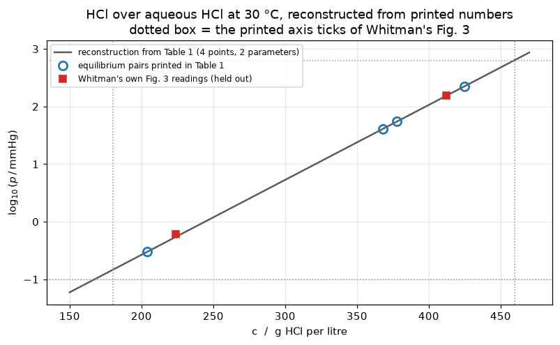

PyMRM implementation

Whitman’s “films” are stagnant layers in which the solute moves by diffusion alone, so the pymrm rendering is not the algebra but the two-domain steady diffusion problem the algebra summarises:

\[\frac{\mathrm{d}}{\mathrm{d}x}\!\left(-k_p \frac{\mathrm{d}p}{\mathrm{d}x}\right) = 0 \quad\text{on the gas film},\qquad \frac{\mathrm{d}}{\mathrm{d}x}\!\left(-k_c \frac{\mathrm{d}c}{\mathrm{d}x}\right) + k_a\,c = 0 \quad\text{on the liquid film},\]

with $p = p_1$ at the outside of the gas film, $c = c_3$ at the inside of the liquid film, and at the interface the two conditions that make it a two-film problem: flux continuity and local equilibrium $p_2 = f(c_2)$. The rate constant $k_a$ is zero for Whitman; it is used only in section 8.

TwoFilm in model.py lays the state out with pymrm.BlockLayout along the one axis that runs through both films: the gas film "p" $(n, 1)$, the two interface values "p2" and "c2" $(1, 1)$, the liquid film "c" $(n, 1)$. Every block of the Jacobian is placed by name (layout.place), the bulk values enter through layout.put, and the interface face of each film is a named subdomain of its faces (its one slice is written once, in _build_operators), selected with pick, so no offset into the state is typed by hand. The two interface values are external unknowns through shapes_d: the boundary value changes every Newton step, so it multiplies a constant boundary matrix and the operators are assembled once. construct_div uses nu=0, a plane film. Both boundary dictionaries are Dirichlet on the outward normal ($a=0$, $b=1$: $b\,\phi = d$, so $\phi = d$ at that end), the physical equation written beside them in model.py.

The system is linear except for $f$ in the single equilibrium row, so its derivative is placed analytically and the Jacobian is exact. Newton starts from the deleted-liquid-film state ($c_2 = c_3$), not from the algebraic answer, with scale= giving every block its physical magnitude, because newton’s step test is absolute and the unknowns are in mmHg and g/l. Each solve is judged by its componentwise backward error (pymrm.checks.residual_check), and the absorption rate is the gas-film flux at the interface face, read with compute_boundary_values.

Film thickness is a gauge. Both films are given unit thickness so that the conductance $D/\delta$ equals Whitman’s printed coefficient. He publishes no area, no thickness and no diffusivity, so nothing else is recoverable and nothing on this page depends on the choice.

The pymrm solve against the algebra: an identity, and labelled as one

A film with constant $D$, Dirichlet ends and no source has a linear profile, and a conservative finite-volume discretisation reproduces it exactly on any grid (the one-sided boundary gradient is exact for a linear profile). So the agreement between TwoFilm.solve and two_film_algebraic below is algebraically guaranteed: it confirms the operator assembly, the shapes_d plumbing, the flux-continuity row and the equilibrium row, and nothing else. It is blind to the grid, and it is not blind to a wrong geometry index or a missing equilibrium jump; the break table shows both.

KP_R3 = float(R[3]["K_p"])                 # Whitman's k_p, the printed K_p of run 3
KC_W = printed("k_c_run1")                 # Whitman's printed k_c, a target only


def worked_kc(eq, kp=KP_R3, runs=R):
    """Whitman's steps 2 to 4: p2 of run 1 from eq. (4), c2 off the curve, then k_c."""
    p2 = runs[1]["p1_mmHg"] - runs[1]["dW_dtheta_g_per_h"] / kp
    c2 = float(eq.c(p2))
    return p2, c2, runs[1]["dW_dtheta_g_per_h"] / (c2 - runs[1]["c3_g_per_l"])


P2_1, C2_1, KC_1 = worked_kc(EQ)
SOLVES = {}
rows = []
for run in (1, 2, 3):
    tf = TwoFilm(KP_R3, KC_1, EQ.p, EQ.dpdc, n=40)
    s, a = tf.solve(P1[run], C3[run]), tf.algebraic(P1[run], C3[run])
    SOLVES[run] = s
    rows.append(dict(run=run, N_pymrm=s["N"], N_algebraic=a["N"],
                     reldev=abs(s["N"] / a["N"] - 1), p2=s["p2"], c2=s["c2"],
                     newton_it=s["nit"], backward_error=s["backward_error"],
                     flux_gap=abs(s["N_liquid_face"] / s["N_gas_face"] - 1)))
port = pd.DataFrame(rows)
display(port[["run", "N_pymrm", "N_algebraic", "p2", "c2", "newton_it"]])
PYMRM_VS_ALG = float(port.reldev.max())
NEWTON_BE_MAX = float(port.backward_error.max())
NEWTON_IT_MAX = int(port.newton_it.max())
FLUX_GAP = float(port.flux_gap.max())
print(f"n = 40 cells per film, k_p = {KP_R3}, k_c = {KC_1:.4f} (Whitman's, derived below)")
print(f"pymrm against the algebra, worst relative deviation: below 1e-11 "
      f"(here {PYMRM_VS_ALG:.1e}), an identity (port check)")
print(f"Newton from the deleted-liquid-film state: at most {NEWTON_IT_MAX} iterations, "
      f"backward error below 1e-12 (here {NEWTON_BE_MAX:.1e})")
print(f"gas and liquid face fluxes at the interface (compute_boundary_values) agree "
      f"below 1e-10 (here {FLUX_GAP:.1e})")
claims.bound("pymrm_vs_algebra_reldev", PYMRM_VS_ALG, max=1e-11, basis="identity",
             note="a linear profile is exact in the finite-volume scheme")
claims.bound("newton_worst_backward_error", NEWTON_BE_MAX, max=1e-12, basis="tolerance",
             note="pymrm.checks.residual_check at the returned state, newton tol 1e-12 scaled")
claims.bound("newton_max_iterations", NEWTON_IT_MAX, max=10, basis="chosen",
             note="exact Jacobian, quadratic convergence from the deleted-liquid-film state")
claims.bound("interface_flux_continuity", FLUX_GAP, max=1e-10, basis="identity",
             note="the flux-continuity row is this equation")


def grid_spread(nu=0):
    """Rate of run 1 on 3, 5, 40 and 600 cells, and its relative spread."""
    out = [(n, TwoFilm(KP_R3, KC_1, EQ.p, EQ.dpdc, n=n, nu=nu).solve(P1[1], C3[1])["N"])
           for n in (3, 5, 40, 600)]
    vals = [v for _, v in out]
    return out, (max(vals) - min(vals)) / abs(np.mean(vals))


GRID, GRID_SPREAD = grid_spread()
print("\ngrid independence, exact on any grid because the profile is linear:")
for n, N in GRID:
    print(f"   n = {n:4d}   N = {N:.9f} g/h")
print(f"   relative spread over n = 3 to 600: below 1e-9 (here {GRID_SPREAD:.1e}), "
      "round-off that grows with the conditioning of the finer grid")
claims.bound("grid_spread_rel_n3_to_n600", GRID_SPREAD, max=1e-9, basis="identity",
             note="no discretisation error; round-off only")

	run	N_pymrm	N_algebraic	p2	c2	newton_it
0	1	41.000000	41.000000	155.508475	412.627200	6
1	2	23.866058	23.866058	0.549054	224.156458	4
2	3	24.189052	24.189052	0.001607	29.429247	3

n = 40 cells per film, k_p = 0.59, k_c = 1.1840 (Whitman's, derived below)
pymrm against the algebra, worst relative deviation: below 1e-11 (here 1.8e-13), an identity (port check)
Newton from the deleted-liquid-film state: at most 6 iterations, backward error below 1e-12 (here 1.5e-16)
gas and liquid face fluxes at the interface (compute_boundary_values) agree below 1e-10 (here 1.3e-13)

grid independence, exact on any grid because the profile is linear:
   n =    3   N = 41.000000000 g/h
   n =    5   N = 41.000000000 g/h
   n =   40   N = 41.000000000 g/h
   n =  600   N = 41.000000002 g/h
   relative spread over n = 3 to 600: below 1e-9 (here 5.9e-11), round-off that grows with the conditioning of the finer grid

Results

1. Whitman’s worked example, reproduced from Table 1 alone

Reprint page 432, in his order:

Take $k_p = K_p(\text{run 3})$, “where the liquid is so dilute that the back pressure $p_2$ is practically zero”.
Use run 1 and eq. (4) to get $p_2$.
Read the matching $c_2$ off Fig. 3.
Hence $k_c$ from eq. (7).
Apply eq. (7) to run 2, solving it together with the equilibrium curve, for run 2’s interface pair.
Hence the run-2 rate, against the observed one.

Step 2 is arithmetic on Table 1 alone, and reproducing it tests only the transcription and eq. (4). Every later step depends on the equilibrium curve, which Whitman read by eye off Fig. 3 and which here comes from the reconstruction: step 3 directly, step 4 through $c_2$, steps 5 and 6 through the pymrm solve. The cell counts the printed numbers compared and how many of them depend on the curve.

def worked_chain(eq, kp=KP_R3, runs=R):
    """Whitman's steps 2 to 6 on a given equilibrium relation, as deviations from his print."""
    p2, c2, kc = worked_kc(eq, kp, runs)
    out = dict(worked_p2_run1_dev_mmHg=abs(p2 - printed("p2_run1")),
               worked_c2_run1_dev_gl=abs(c2 - printed("c2_run1")))
    if not kc > 0:                                  # c2 below c3: no solution
        return out | dict(worked_kc_reldev=np.nan, run2_c2_dev_gl=np.nan,
                          run2_p2_dev_mmHg=np.nan, run2_rate_reldev=np.nan), None
    s = TwoFilm(kp, kc, eq.p, eq.dpdc, n=40).solve(runs[2]["p1_mmHg"], runs[2]["c3_g_per_l"])
    out |= dict(worked_kc_reldev=abs(kc / printed("k_c_run1") - 1),
                run2_c2_dev_gl=abs(s["c2"] - printed("c2_run2")),
                run2_p2_dev_mmHg=abs(s["p2"] - printed("p2_run2")),
                run2_rate_reldev=abs(s["N"] / runs[2]["dW_dtheta_g_per_h"] - 1))
    return out, s


WORKED, R2 = worked_chain(EQ)
comp = pd.DataFrame([
    ("p2, run 1  (mmHg)", P2_1, printed("p2_run1"), "derived by Whitman"),
    ("c2, run 1  (g/l)", C2_1, printed("c2_run1"), "read by Whitman off Fig. 3"),
    ("k_c        (g/h/(g/l))", KC_1, printed("k_c_run1"), "derived by Whitman"),
    ("p2, run 2  (mmHg)", R2["p2"], printed("p2_run2"), "read by Whitman off Fig. 3"),
    ("c2, run 2  (g/l)", R2["c2"], printed("c2_run2"), "read by Whitman off Fig. 3"),
    ("dW/dth run 2 (g/h)", R2["N"], printed("rate_run2_predicted"),
     f"Whitman's prediction; the observed rate is {OBS[2]}"),
], columns=["quantity", "this page", "Whitman", "what it is"])
comp["deviation"] = comp["this page"] - comp["Whitman"]
comp["reldev_%"] = 100 * (comp["this page"] / comp["Whitman"] - 1)
display(comp.round(4))
print(f"{len(comp)} printed numbers compared; {len(comp) - 1} of them depend on the "
      "reconstructed curve (all but p2 of run 1)")
for k, v in WORKED.items():
    claims.value(k, v, rtol=0.01)
print(f"held-out run-2 rate: {R2['N']:.3f} g/h against the observed {OBS[2]} "
      f"({100 * (R2['N'] / OBS[2] - 1):+.3f} %)")
print(f"\nrun 2's interface pressure is the one large relative deviation "
      f"({100 * (R2['p2'] / printed('p2_run2') - 1):+.1f} %): Whitman read "
      f"{printed('p2_run2')} mmHg where this gives {R2['p2']:.3f}.")
print(f"On his Fig. 3 that is {abs(np.log10(R2['p2'] / printed('p2_run2'))):.3f} log units "
      f"on an ordinate spanning {O_HI - O_LO:.1f}: a chart-reading difference, and it "
      f"costs {abs(R2['c2'] - printed('c2_run2')):.2f} g/l in c2.")

	quantity	this page	Whitman	what it is	deviation	reldev_%
0	p2, run 1 (mmHg)	155.5085	156.0	derived by Whitman	-0.4915	-0.3151
1	c2, run 1 (g/l)	412.6272	412.0	read by Whitman off Fig. 3	0.6272	0.1522
2	k_c (g/h/(g/l))	1.1840	1.2	derived by Whitman	-0.0160	-1.3300
3	p2, run 2 (mmHg)	0.5491	0.6	read by Whitman off Fig. 3	-0.0509	-8.4909
4	c2, run 2 (g/l)	224.1565	224.0	read by Whitman off Fig. 3	0.1565	0.0698
5	dW/dth run 2 (g/h)	23.8661	24.0	Whitman's prediction; the observed rate is 24.0	-0.1339	-0.5581

6 printed numbers compared; 5 of them depend on the reconstructed curve (all but p2 of run 1)
held-out run-2 rate: 23.866 g/h against the observed 24.0 (-0.558 %)

run 2's interface pressure is the one large relative deviation (-8.5 %): Whitman read 0.6 mmHg where this gives 0.549.
On his Fig. 3 that is 0.039 log units on an ordinate spanning 3.8: a chart-reading difference, and it costs 0.16 g/l in c2.

2. How much of that prediction is the liquid film?

The run-2 check is the only prediction in the paper: $k_p$ comes from run 3, $k_c$ from run 1, and run 2’s rate is never used to obtain either. That makes it the right thing to look at, and the wrong thing to be reassured by.

Run 2 is a dilute acid, where the back pressure is a fraction of a mmHg against a bulk gas pressure of tens. The interface barely backs up, so almost the whole resistance sits in the gas film. The table below fixes $k_p$ and sweeps $k_c$, ending with $k_c \to \infty$: deleting the liquid film entirely.

That last row is taken analytically, not by putting a large number in $k_c$. With no liquid resistance the interface concentration is the bulk concentration, so the limit is the closed form $k_p\,(p_1 - f(c_3))$ with no tuning constant in it.

def resistance_share(eq, kc, run, kp=KP_R3):
    """Fraction of the total driving force (p1 - f(c3)) that drops across the gas film."""
    s = two_film_algebraic(P1[run], C3[run], kp, kc, eq.p)
    return (P1[run] - s["p2"]) / (P1[run] - float(eq.p(C3[run])))


SHARE = {run: resistance_share(EQ, KC_1, run) for run in (1, 2)}
print(f"gas-film share of the total resistance:  run 2 {100 * SHARE[2]:.2f} %   "
      f"run 1 {100 * SHARE[1]:.2f} %")
claims.value("run2_gasfilm_resistance_share", SHARE[2], rtol=1e-3)
claims.value("run1_gasfilm_resistance_share", SHARE[1], rtol=1e-3)


def run2_rate(kc, kp=KP_R3, eq=EQ):
    return two_film_algebraic(P1[2], C3[2], kp, kc, eq.p)


NO_LF = no_liquid_film_rate(P1[2], C3[2], KP_R3, EQ.p)        # the k_c -> infinity limit
rows = []
for lab, f in [("k_c / 8", 1 / 8), ("k_c / 4", 1 / 4), ("k_c / 2", 1 / 2),
               ("k_c as derived", 1.0), ("k_c x 2", 2.0), ("k_c x 10", 10.0),
               ("k_c x 1000", 1000.0)]:
    s = run2_rate(f * KC_1)
    rows.append(dict(case=lab, k_c=f * KC_1, c2=s["c2"], p2=s["p2"], rate=s["N"],
                     dev_vs_observed_pct=100 * (s["N"] / OBS[2] - 1)))
rows.append(dict(case="k_c -> infinity, closed form (NO liquid film)", k_c=np.inf,
                 c2=NO_LF["c2"], p2=NO_LF["p2"], rate=NO_LF["N"],
                 dev_vs_observed_pct=100 * (NO_LF["N"] / OBS[2] - 1)))
display(pd.DataFrame(rows).round(6))
NO_LIQUID_RELDEV = abs(NO_LF["N"] / OBS[2] - 1)
LF_EFFECT = NO_LF["N"] / R2["N"] - 1
print(f"\nWith the liquid film DELETED, run 2's predicted rate is {NO_LF['N']:.4f} g/h, "
      f"{100 * (NO_LF['N'] / OBS[2] - 1):+.4f} % from the observed {OBS[2]}.")
print(f"With Whitman's k_c = {KC_1:.3f} it is {R2['N']:.4f} g/h, "
      f"{100 * (R2['N'] / OBS[2] - 1):+.4f} %: the liquid film moves it by "
      f"{100 * LF_EFFECT:.2f} %.")
print(f"Table 1 prints the rate to 0.1 g/h, +-{100 * RATE_HALF_UNIT / OBS[2]:.2f} %.")
print("\nSo the paper's one held-out prediction cannot distinguish a liquid film")
print("from no liquid film, and of the two the NO-liquid-film answer is closer.")
claims.value("run2_rate_reldev_no_liquid_film", NO_LIQUID_RELDEV, rtol=0.01)
claims.value("run2_liquid_film_effect", LF_EFFECT, rtol=0.01)

gas-film share of the total resistance:  run 2 99.39 %   run 1 40.90 %

	case	k_c	c2	p2	rate	dev_vs_observed_pct
0	k_c / 8	0.148005	323.942053	10.911817	17.752028	-26.033217
1	k_c / 4	0.296010	279.905854	2.917123	22.468897	-6.379594
2	k_c / 2	0.592020	243.872343	0.991136	23.605230	-1.644875
3	k_c as derived	1.184040	224.156458	0.549054	23.866058	-0.558092
4	k_c x 2	2.368081	214.113771	0.406399	23.950224	-0.207398
5	k_c x 10	11.840403	206.027111	0.318962	24.001812	0.007551
6	k_c x 1000	1184.040291	204.020280	0.300351	24.012793	0.053303
7	k_c -> infinity, closed form (NO liquid film)	inf	204.000000	0.300169	24.012900	0.053752


With the liquid film DELETED, run 2's predicted rate is 24.0129 g/h, +0.0538 % from the observed 24.0.
With Whitman's k_c = 1.184 it is 23.8661 g/h, -0.5581 %: the liquid film moves it by 0.62 %.
Table 1 prints the rate to 0.1 g/h, +-0.21 %.

So the paper's one held-out prediction cannot distinguish a liquid film
from no liquid film, and of the two the NO-liquid-film answer is closer.

The same limit, computed a second way

The number above is the page’s headline, so it is computed twice, by routes that share the gas-side expression $k_p\,(p_1 - f(\cdot))$ and no solver.

Route A, used above: the closed form $k_p\,(p_1 - f(c_3))$. One multiplication; no root is solved.
Route B: solve the full two-film problem by brentq at two finite, well-conditioned values of $k_c$ and extrapolate. The leading correction is $N(k_c) = N_\infty - a/k_c + O(k_c^{-2})$, because raising the interface by $\delta c = N/k_c$ raises the back pressure by $f'(c_3)\,\delta c$, so two points a decade apart eliminate it: $N_\infty \approx \bigl(10\,N(10k) - N(k)\bigr)/9$.

Then what happens if the limit is taken the obvious way instead: by setting $k_c$ to a large constant and reading the rate off the liquid side of eq. (4).

def route_b(k, extrapolate=True):
    """Deleted-liquid-film rate of run 2 from finite k and 10 k (Richardson in 1/k_c)."""
    n1, n10 = run2_rate(k)["N"], run2_rate(10 * k)["N"]
    return (10 * n10 - n1) / 9.0 if extrapolate else n10


K_A = KC_1 * 1e4
NB = route_b(K_A)
NO_LF_TWO_ROUTES = abs(NB / NO_LF["N"] - 1)
print("run 2 with the liquid film deleted, two routes:")
print(f"   A  closed form  k_p (p1 - f(c3))              {NO_LF['N']:.9f} g/h")
print(f"   B  Richardson on k_c = 1e4 and 1e5 x derived  {NB:.9f} g/h")
print(f"   relative difference below 1e-10 (here {NO_LF_TWO_ROUTES:.1e})")
claims.bound("no_liquid_film_two_routes", NO_LF_TWO_ROUTES, max=1e-10, basis="tolerance",
             note="brentq xtol 1e-13 on c2, O(1/k_c^2) remainder at k_c = 1e4 derived")

run 2 with the liquid film deleted, two routes:
   A  closed form  k_p (p1 - f(c3))              24.012900453 g/h
   B  Richardson on k_c = 1e4 and 1e5 x derived  24.012900453 g/h
   relative difference below 1e-10 (here 1.3e-12)

And why the obvious route is wrong

Eq. (4) says $k_p(p_1-p_2) = k_c(c_2-c_3)$, so it looks as though either side may be evaluated. They are not equally conditioned. As $k_c$ grows, $c_2-c_3$ shrinks like $1/k_c$ while $c_2$ itself stays at the bulk value, where consecutive representable doubles are $\mathrm{ulp}(c_3)$ apart. The liquid-side product $k_c(c_2-c_3)$ therefore comes in steps of $k_c\,\mathrm{ulp}(c_3)$, a quantisation that grows with $k_c$ while the quantity it is quantising does not. The table prints the step beside the answer. The signature is visible without knowing any of that: the liquid-side value can exceed the exact $k_c\to\infty$ limit, which a rate increasing in $k_c$ cannot do.

ULP = float(np.spacing(C3[2]))
rows = []
for kc in [1e9, 1e10, 1e11, 1e12, 1e13]:
    s = run2_rate(kc)
    rows.append(dict(k_c=kc, c2_minus_c3=s["c2"] - C3[2], quantisation_g_per_h=kc * ULP,
                     rate_gas_side=s["N"], rate_liquid_side=s["N_liquid_side"],
                     exceeds_the_limit=bool(s["N_liquid_side"] > NO_LF["N"])))
display(pd.DataFrame(rows))
print(f"exact k_c -> infinity limit {NO_LF['N']:.6f} g/h;  ulp({C3[2]:g}) = {ULP:.3e} g/l")
print(f"the quantity being reported, the deleted-film rate minus the observed one, is "
      f"{abs(NO_LF['N'] - OBS[2]):.4f} g/h,")
print(f"against a liquid-side quantisation of {1e12 * ULP:.4f} g/h at k_c = 1e12, "
      f"{1e12 * ULP / abs(NO_LF['N'] - OBS[2]):.1f} times larger.")
print("The gas-side column is flat over four decades of k_c; the liquid-side column")
print("is not, and no value of k_c is used anywhere above.")

	k_c	c2_minus_c3	quantisation_g_per_h	rate_gas_side	rate_liquid_side	exceeds_the_limit
0	1.000000e+09	2.401291e-08	0.000028	24.0129	24.012905	True
1	1.000000e+10	2.401293e-09	0.000284	24.0129	24.012934	True
2	1.000000e+11	2.401350e-10	0.002842	24.0129	24.013502	True
3	1.000000e+12	2.401634e-11	0.028422	24.0129	24.016344	True
4	1.000000e+13	2.387424e-12	0.284217	24.0129	23.874236	False

exact k_c -> infinity limit 24.012900 g/h;  ulp(204) = 2.842e-14 g/l
the quantity being reported, the deleted-film rate minus the observed one, is 0.0129 g/h,
against a liquid-side quantisation of 0.0284 g/h at k_c = 1e12, 2.2 times larger.
The gas-side column is flat over four decades of k_c; the liquid-side column
is not, and no value of k_c is used anywhere above.

# The classical two-film diagram: ONE potential across both films. In the gas
# film that is the partial pressure itself; in the liquid film it is the
# pressure the local concentration would exert, f(c). The two meet at the
# interface by construction, so the drop across each film is directly readable.
fig, axes = plt.subplots(1, 2, figsize=(11.2, 4.2))
for ax, run in zip(axes, (1, 2)):
    tf = TwoFilm(KP_R3, KC_1, EQ.p, EQ.dpdc, n=60)
    s = tf.solve(P1[run], C3[run])
    x_c = 0.5 * (tf.x_f[1:] + tf.x_f[:-1])
    ax.plot(x_c, s["p"] / P1[run], "-", lw=2.2, color="C0", label="gas film: $p$")
    ax.plot(1 + x_c, EQ.p(s["c"]) / P1[run], "-", lw=2.2, color="C3",
            label=r"liquid film: $f(c)$")
    ax.axvline(1.0, color="0.4", lw=1.2)
    ax.axhline(float(EQ.p(C3[run])) / P1[run], ls=":", lw=1, color="0.5")
    ax.set_xlabel("gas film                    |                    liquid film")
    ax.set_ylim(0, 1.05)
    ax.set_title(f"run {run}: $c_3$ = {C3[run]:g} g/l\ngas film carries "
                 f"{100 * resistance_share(EQ, KC_1, run):.1f} % of the resistance", fontsize=10)
    ax.set_xticks([])
    ax.legend(fontsize=8, loc="lower left")
axes[0].set_ylabel(r"potential  $p\,/\,p_1$")
fig.suptitle("Where the resistance sits, at Whitman's own two extremes", y=1.02)
fig.tight_layout()
plt.show()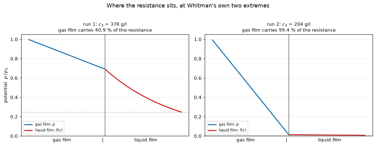

3. The three runs against three models

This is the comparison with power. Three published rates; three candidate models, each fitted to all three runs by least squares on the relative residual in $\mathrm{d}W/\mathrm{d}\theta$:

single gas film, eq. (5) with a constant $K_p = k_p$: one parameter;
single liquid film, eq. (6) with a constant $K_c = k_c$: one parameter;
two films, eq. (4) closed with the reconstructed equilibrium curve: two parameters, so one degree of freedom remains.

Two of these three numbers were settled before any physics entered, and the page should say which. The two-film family nests the single-gas-film model: $k_c \to \infty$ is eq. (5) with the back pressure taken from the equilibrium curve instead of from Table 1’s $p_3$ column. Its second parameter is then free to absorb run 1, the only run with a real liquid resistance, and it does, to a residual of a few thousandths of a per cent. So the three-run rms is set by runs 2 and 3, and their mutual consistency under one gas coefficient is already printed in Table 1, as the same $K_p$ for both. The two-film rms could not have come out at tens of per cent.

What could fail is the one degree of freedom that is left over, and section 4 shows that it does, and that the liquid film makes it worse.

def rel_resid_two(theta, kc=None, subset=(1, 2, 3), runs=RUNS, eq=EQ):
    kp = np.exp(theta[0])
    kcv = np.exp(theta[1]) if kc is None else kc
    return [two_film_algebraic(r["p1_mmHg"], r["c3_g_per_l"], kp, kcv, eq.p)["N"]
            / r["dW_dtheta_g_per_h"] - 1 for r in runs if int(r["run"]) in subset]


def rel_resid_gas(theta, subset=(1, 2, 3), runs=RUNS):
    kp = np.exp(theta[0])
    return [kp * (r["p1_mmHg"] - r["p3_mmHg"]) / r["dW_dtheta_g_per_h"] - 1
            for r in runs if int(r["run"]) in subset]


def rel_resid_nolf(theta, subset=(1, 2, 3), runs=RUNS, eq=EQ):
    """The two-film family's k_c -> infinity member: one parameter, k_p."""
    kp = np.exp(theta[0])
    return [no_liquid_film_rate(r["p1_mmHg"], r["c3_g_per_l"], kp, eq.p)["N"]
            / r["dW_dtheta_g_per_h"] - 1 for r in runs if int(r["run"]) in subset]


def rel_resid_liq(theta, runs=RUNS):
    kc = np.exp(theta[0])
    return [kc * (r["c1_g_per_l"] - r["c3_g_per_l"]) / r["dW_dtheta_g_per_h"] - 1
            for r in runs]


def fit(f, x0):
    s = least_squares(f, x0)
    r = np.asarray(f(s.x))
    return np.exp(s.x), r, float(np.sqrt((r ** 2).mean()))


par_g, res_g, rms_g = fit(rel_resid_gas, [np.log(0.4)])
par_l, res_l, rms_l = fit(rel_resid_liq, [np.log(0.3)])
par_2, res_2, rms_2 = fit(rel_resid_two, np.log([0.59, 1.2]))
display(pd.DataFrame([
    dict(model="single gas film, eq. (5)", n_par=1, fitted=f"k_p = {par_g[0]:.4f}",
         rms_pct=100 * rms_g, worst_pct=100 * np.abs(res_g).max()),
    dict(model="single liquid film, eq. (6)", n_par=1, fitted=f"k_c = {par_l[0]:.4f}",
         rms_pct=100 * rms_l, worst_pct=100 * np.abs(res_l).max()),
    dict(model="two films, eq. (4)", n_par=2,
         fitted=f"k_p = {par_2[0]:.4f}, k_c = {par_2[1]:.4f}",
         rms_pct=100 * rms_2, worst_pct=100 * np.abs(res_2).max())]).round(3))
print("per-run relative residuals, %")
print(f"   single gas film    {np.round(100 * res_g, 2)}")
print(f"   single liquid film {np.round(100 * res_l, 2)}")
print(f"   two films          {np.round(100 * res_2, 3)}")
print(f"\nTable 1's own precision on a rate is +-{100 * RATE_HALF_UNIT / OBS[2]:.2f} %.")
print("A single film, either one, misses by tens of per cent. Two films do not.")
claims.value("gasfilm_3run_rms_pct", 100 * rms_g, rtol=1e-3)
claims.value("liquidfilm_3run_rms_pct", 100 * rms_l, rtol=1e-3)
claims.value("twofilm_3run_rms_pct", 100 * rms_2, rtol=1e-3)
claims.value("gasfilm_3run_worst_pct", 100 * np.abs(res_g).max(), rtol=1e-3)
claims.value("liquidfilm_3run_worst_pct", 100 * np.abs(res_l).max(), rtol=1e-3)
claims.value("twofilm_3run_worst_pct", 100 * np.abs(res_2).max(), rtol=1e-3)
claims.value("twofilm_run1_resid_pct", 100 * abs(res_2[0]), rtol=0.05)

	model	n_par	fitted	rms_pct	worst_pct
0	single gas film, eq. (5)	1	k_p = 0.3285	41.708	44.289
1	single liquid film, eq. (6)	1	k_c = 0.0848	59.474	90.284
2	two films, eq. (4)	2	k_p = 0.5905, k_c = 1.1837	0.379	0.470

per-run relative residuals, %
   single gas film    [ 36.21 -44.29 -44.11]
   single liquid film [-90.28 -42.08  26.25]
   two films          [ 0.005 -0.47   0.46 ]

Table 1's own precision on a rate is +-0.21 %.
A single film, either one, misses by tens of per cent. Two films do not.

How much of the two-film rms was available to fail

Run 1’s two-film residual is the smallest of the three, because $k_c$ is the parameter that fits it. Strip run 1 out and what remains is a two-point, one-parameter problem, whose residual is fixed by how well runs 2 and 3 agree under a single gas coefficient: a number Table 1 prints directly, as $K_p$ twice.

KP_COL = {run: OBS[run] / float(R[run]["delta_p_mmHg"]) for run in (2, 3)}
RUNS23_KP_DISAGREE = KP_COL[2] / KP_COL[3] - 1
print(f"Table 1's K_p column, recomputed: run 2 {KP_COL[2]:.5f}, run 3 {KP_COL[3]:.5f}, "
      f"both printed as {R[2]['K_p']}")
print(f"   they disagree by {100 * RUNS23_KP_DISAGREE:.3f} %, and that is the whole budget")
print("   any one-parameter gas model has to work with on these two runs.\n")
par_g23, res_g23, rms_g23 = fit(lambda th: rel_resid_gas(th, subset=(2, 3)), [np.log(0.59)])
par_n23, res_n23, rms_n23 = fit(lambda th: rel_resid_nolf(th, subset=(2, 3)), [np.log(0.59)])
res_2_23 = np.asarray(res_2)[[1, 2]]
TWOFILM_RUNS23_RMS = float(np.sqrt((res_2_23 ** 2).mean()) * 100)
display(pd.DataFrame([
    dict(model="single gas film, eq. (5), printed p3", n_par=1,
         fitted=f"k_p = {par_g23[0]:.5f}", rms_pct=100 * rms_g23,
         resid_run2_pct=100 * res_g23[0], resid_run3_pct=100 * res_g23[1]),
    dict(model="liquid film DELETED (k_c -> inf), f(c3)", n_par=1,
         fitted=f"k_p = {par_n23[0]:.5f}", rms_pct=100 * rms_n23,
         resid_run2_pct=100 * res_n23[0], resid_run3_pct=100 * res_n23[1]),
    dict(model="two films (k_p, k_c fitted to all three)", n_par=2,
         fitted=f"k_p = {par_2[0]:.5f}, k_c = {par_2[1]:.5f}", rms_pct=TWOFILM_RUNS23_RMS,
         resid_run2_pct=100 * res_2_23[0], resid_run3_pct=100 * res_2_23[1])]).round(4))
KP_F, KC_F = par_2
FIT_R2 = two_film_algebraic(P1[2], C3[2], KP_F, KC_F, EQ.p)
print(f"On the only two runs that constrain k_p, a ONE-parameter gas film fits to "
      f"{100 * rms_g23:.3f} % rms")
print(f"and the two-parameter two-film model to {TWOFILM_RUNS23_RMS:.3f} %, "
      f"{TWOFILM_RUNS23_RMS / (100 * rms_g23):.2f} times worse.")
print("Adding the liquid film degrades these two runs, because the fit to run 1 backs")
print(f"run 2's interface up from f(c3) = {float(EQ.p(C3[2])):.3f} to "
      f"{FIT_R2['p2']:.3f} mmHg.")
claims.value("gasfilm_runs23_rms_pct", 100 * rms_g23, rtol=1e-3)
claims.value("nolf_runs23_rms_pct", 100 * rms_n23, rtol=1e-3)
claims.value("twofilm_runs23_rms_pct", TWOFILM_RUNS23_RMS, rtol=1e-3)
claims.value("twofilm_fit_run2_p2_mmHg", FIT_R2["p2"], rtol=1e-3)

Table 1's K_p column, recomputed: run 2 0.58968, run 3 0.58780, both printed as 0.59
   they disagree by 0.319 %, and that is the whole budget
   any one-parameter gas model has to work with on these two runs.

	model	n_par	fitted	rms_pct	resid_run2_pct	resid_run3_pct
0	single gas film, eq. (5), printed p3	1	k_p = 0.58874	0.1593	-0.1596	0.1590
1	liquid film DELETED (k_c -> inf), f(c3)	1	k_p = 0.58875	0.1584	-0.1587	0.1582
2	two films (k_p, k_c fitted to all three)	2	k_p = 0.59053, k_c = 1.18367	0.4647	-0.4696	0.4598

On the only two runs that constrain k_p, a ONE-parameter gas film fits to 0.159 % rms
and the two-parameter two-film model to 0.465 %, 2.92 times worse.
Adding the liquid film degrades these two runs, because the fit to run 1 backs
run 2's interface up from f(c3) = 0.300 to 0.549 mmHg.

4. Where the one degree of freedom lands, and it does not land cleanly

Three observations minus two parameters leaves one testable combination, and it is essentially the ratio of run 3’s rate to run 2’s. Both runs share $p_1$; they differ only in bulk liquid concentration. Two-film theory says run 3 must be the faster of the two, because run 2’s interface backs up to a finite partial pressure and run 3’s does not. The question is by how much.

$k_p$ cancels out of a ratio of two runs at the same $p_1$, so three of the four predictions below contain no fitted parameter at all: they are properties of the model, not of the fit. That makes this the cleanest comparison the data allow.

def dof_ratios(eq=EQ, kc=KC_F, kp=KP_F, runs=R):
    """run3/run2 rate ratio: observed, and as four models predict it."""
    p1_2, p1_3 = runs[2]["p1_mmHg"], runs[3]["p1_mmHg"]
    c3_2, c3_3 = runs[2]["c3_g_per_l"], runs[3]["c3_g_per_l"]
    two = (two_film_algebraic(p1_3, c3_3, kp, kc, eq.p)["N"]
           / two_film_algebraic(p1_2, c3_2, kp, kc, eq.p)["N"])
    return dict(
        observed=runs[3]["dW_dtheta_g_per_h"] / runs[2]["dW_dtheta_g_per_h"],
        none=p1_3 / p1_2,
        gas=(p1_3 - runs[3]["p3_mmHg"]) / (p1_2 - runs[2]["p3_mmHg"]),
        nolf=(no_liquid_film_rate(p1_3, c3_3, kp, eq.p)["N"]
              / no_liquid_film_rate(p1_2, c3_2, kp, eq.p)["N"]),
        two=two)


RAT = dof_ratios()
PREC_RATIO = 100 * np.hypot(RATE_HALF_UNIT / OBS[2], RATE_HALF_UNIT / OBS[3])
labels = dict(none=("no back pressure at all", "no parameters"),
              gas=("single gas film, eq. (5), Table 1's p3", "no parameters"),
              nolf=("liquid film deleted, back pressure from f(c3)", "no parameters (k_p cancels)"),
              two=("two films, fitted k_c", "k_c enters; k_p cancels"))
display(pd.DataFrame([dict(model=labels[k][0], run3_over_run2=RAT[k],
                           dev_vs_table1_pct=100 * (RAT[k] / RAT["observed"] - 1),
                           free=labels[k][1]) for k in labels]).round(5))
DOF_OVERPRED_PCT = 100 * (RAT["two"] / RAT["observed"] - 1)
GASFILM_DOF_PCT = 100 * (RAT["gas"] / RAT["observed"] - 1)
GAP_FRACTION = (RAT["observed"] - 1) / (RAT["two"] - 1)
print(f"Table 1:  run3/run2 = {RAT['observed']:.5f}, printed precision +-{PREC_RATIO:.2f} %")
print(f"The observed gap sits BETWEEN no back pressure "
      f"({100 * (RAT['none'] / RAT['observed'] - 1):+.3f} %) and a gas film alone "
      f"({GASFILM_DOF_PCT:+.3f} %).")
print(f"The two-film model over-predicts it by {DOF_OVERPRED_PCT:+.3f} %: the observed gap "
      f"is {GAP_FRACTION:.2f} of the predicted one.")
KP_IDENTITY = abs(GASFILM_DOF_PCT / 100 - RUNS23_KP_DISAGREE)
print(f"\n{GASFILM_DOF_PCT:+.3f} % is the {100 * RUNS23_KP_DISAGREE:.3f} % by which Table 1's "
      "two K_p, recomputed from its delta_p column, disagree (gap below 1e-12, "
      f"here {KP_IDENTITY:.1e}):")
print("K_p(run 2)/K_p(run 3) = (N2/N3)(dp3/dp2). One number, seen twice.")
claims.value("ratio_observed_run3_over_run2", RAT["observed"], rtol=1e-5)
claims.value("ratio_twofilm_run3_over_run2", RAT["two"], rtol=1e-5)
claims.value("ratio_gasfilm_run3_over_run2", RAT["gas"], rtol=1e-5)
claims.value("ratio_nolf_run3_over_run2", RAT["nolf"], rtol=1e-5)
claims.value("dof_ratio_overpredict_pct", DOF_OVERPRED_PCT, rtol=1e-3)
claims.value("gasfilm_dof_ratio_dev_pct", GASFILM_DOF_PCT, rtol=1e-3)
claims.value("dof_gap_fraction", GAP_FRACTION, rtol=1e-3)
claims.bound("kp_disagreement_is_gasfilm_dof", KP_IDENTITY, max=1e-12, basis="identity",
             note="K_p(2)/K_p(3) - 1 and the gas-film ratio deviation "
             "are the same expression")
print("\nand the ratio barely depends on k_c, so this test does not probe it either:")
for lab, k in [(f"{KC_F:9.4g}", KC_F), (f"{5 * KC_F:9.4g}", 5 * KC_F)]:
    print(f"     k_c = {lab}   run3/run2 = {dof_ratios(kc=k)['two']:.5f}")
print(f"     k_c = infinity    run3/run2 = {RAT['nolf']:.5f}")

	model	run3_over_run2	dev_vs_table1_pct	free
0	no back pressure at all	1.00000	-0.41494	no parameters
1	single gas film, eq. (5), Table 1's p3	1.00737	0.31910	no parameters
2	liquid film deleted, back pressure from f(c3)	1.00735	0.31739	no parameters (k_p cancels)
3	two films, fitted k_c	1.01354	0.93380	k_c enters; k_p cancels

Table 1:  run3/run2 = 1.00417, printed precision +-0.29 %
The observed gap sits BETWEEN no back pressure (-0.415 %) and a gas film alone (+0.319 %).
The two-film model over-predicts it by +0.934 %: the observed gap is 0.31 of the predicted one.

+0.319 % is the 0.319 % by which Table 1's two K_p, recomputed from its delta_p column, disagree (gap below 1e-12, here 2.2e-16):
K_p(run 2)/K_p(run 3) = (N2/N3)(dp3/dp2). One number, seen twice.

and the ratio barely depends on k_c, so this test does not probe it either:
     k_c =     1.184   run3/run2 = 1.01354
     k_c =     5.918   run3/run2 = 1.00831
     k_c = infinity    run3/run2 = 1.00735

So the single quantitative test the data offer is not passed cleanly: the observed gap between runs 2 and 3 is about a third of the predicted one, a discrepancy of order 1 % against a printed precision of order 0.3 %. It is far too small to refute anything (Whitman quotes no experimental error, and 1 % on a 1923 absorption rate is nothing), but it is worth being exact about what it says. On both quantities the three runs can actually test (the held-out run-2 rate of section 2, and this ratio) the two-film model is beaten by the same model with the liquid film taken out, which has one parameter fewer. That is the same finding twice, and it points the same way as everything else on this page: the data show less liquid-film effect than the theory needs.

5. What the three runs can say about the liquid-film coefficient, and what they cannot

Profile the fit: fix $k_c$, re-fit $k_p$, and look at the residual. Do it for every subset of two or three runs. The band of $k_c$ a subset admits is where its rms stays below 2 %, about ten times Table 1’s own precision on a rate; its edges are root-found on the profile, not read off the sweep.

THRESH = 0.02                           # 2 % rms
KC_SWEEP = np.geomspace(0.3, 3e3, 160)


def profile_rms(kc, subset, runs=RUNS, eq=EQ):
    """rms relative residual with k_c fixed and k_p re-fitted."""
    s = least_squares(lambda th: rel_resid_two(th, kc=kc, subset=subset, runs=runs, eq=eq),
                      [np.log(0.59)], xtol=1e-14, ftol=1e-14, gtol=1e-14)
    r = np.asarray(rel_resid_two(s.x, kc=kc, subset=subset, runs=runs, eq=eq))
    return float(np.sqrt((r ** 2).mean()))


def kc_band(subset, runs=RUNS, eq=EQ):
    """Root-found edges of {k_c: profile rms <= THRESH}; the upper edge is inf when the
    rms is still below THRESH at the top of the sweep."""
    v = np.array([profile_rms(k, subset, runs, eq) for k in KC_SWEEP]) - THRESH
    inside = np.flatnonzero(v <= 0)
    if inside.size == 0:
        return np.nan, np.nan, v + THRESH
    i, j = inside[0], inside[-1]
    if not np.all(v[i:j + 1] <= 0):
        raise ValueError(f"the admitted set of {subset} is not one interval")

    def g(k):
        return profile_rms(k, subset, runs, eq) - THRESH

    lo = KC_SWEEP[0] if i == 0 else brentq(g, KC_SWEEP[i - 1], KC_SWEEP[i], xtol=1e-12)
    hi = np.inf if j == len(KC_SWEEP) - 1 else brentq(g, KC_SWEEP[j], KC_SWEEP[j + 1],
                                                     xtol=1e-12)
    return lo, hi, v + THRESH


SUBSETS = [((1, 2, 3), "all three runs"), ((1, 2), "runs 1 and 2"),
           ((1, 3), "runs 1 and 3"), ((2, 3), "runs 2 and 3, run 1 REMOVED")]
BANDS, PROF = {}, {}
for sub, lab in SUBSETS:
    lo, hi, PROF[sub] = kc_band(sub)
    BANDS[sub] = (lo, hi)
    top = ("  still below 2 % at the top of the sweep" if not np.isfinite(hi) else "")
    print(f"  {lab:30s}: k_c admitted at rms <= {100 * THRESH:.0f} %: "
          f"[{lo:.3g}, {hi:.4g}]{top}")
WITH_RUN1 = [s for s, _ in SUBSETS if 1 in s]
KC_LO_RUN1 = min(BANDS[s][0] for s in WITH_RUN1)
KC_HI_RUN1 = max(BANDS[s][1] for s in WITH_RUN1)
KC_BAND_WIDTH_ALL = BANDS[(1, 2, 3)][1] / BANDS[(1, 2, 3)][0]
P23 = PROF[(2, 3)]
print(f"\n  every subset containing run 1 admits k_c only in [{KC_LO_RUN1:.3f}, "
      f"{KC_HI_RUN1:.3f}]; with all three runs the band spans a factor "
      f"{KC_BAND_WIDTH_ALL:.4f}")
UNBOUNDED_NO1 = bool(np.isinf(BANDS[(2, 3)][1]))
RISES_NO1 = int(np.sum(np.diff(P23) > 0))
print(f"  with run 1 removed the band starts at {BANDS[(2, 3)][0]:.3f}; upper end "
      f"{'none' if UNBOUNDED_NO1 else 'finite'}: the profile has {RISES_NO1} rises in "
      f"{len(P23) - 1} steps")
print(f"  towards its k_c -> infinity limit, the deleted-film fit, {100 * rms_n23:.3f} % rms")
claims.exact("kc_band_without_run1_unbounded", UNBOUNDED_NO1)
claims.exact("profile_without_run1_rises", RISES_NO1)
claims.value("kc_band_low_all_runs", BANDS[(1, 2, 3)][0], rtol=1e-4)
claims.value("kc_band_high_all_runs", BANDS[(1, 2, 3)][1], rtol=1e-4)
claims.value("kc_band_width_all_runs", KC_BAND_WIDTH_ALL, rtol=1e-4)
claims.value("kc_band_low_run1_subsets", KC_LO_RUN1, rtol=1e-4)
claims.value("kc_band_high_run1_subsets", KC_HI_RUN1, rtol=1e-4)
claims.value("kc_band_low_without_run1", BANDS[(2, 3)][0], rtol=1e-4)

fig, ax = plt.subplots(figsize=(7.6, 4.4))
for (sub, lab), st in zip(SUBSETS, ["-", "--", "-.", "-"]):
    ax.loglog(KC_SWEEP, 100 * PROF[sub], st, lw=2.2 if len(sub) != 2 else 1.4, label=lab)
ax.axhline(100 * THRESH, ls=":", lw=1.2, color="0.4",
           label=f"{100 * THRESH:.0f} % rms threshold")
ax.axvline(KC_F, ls=(0, (6, 3)), lw=1.4, color="0.15", label=f"fitted $k_c$ = {KC_F:.2f}")
ax.set_xlabel(r"$k_c$  /  g h$^{-1}$ (g/l)$^{-1}$   (held fixed; $k_p$ re-fitted at each point)")
ax.set_ylabel(r"rms relative residual in $dW/d\theta$  /  %")
ax.set_title("Every subset containing run 1 pins $k_c$; the one without it does not")
ax.legend(fontsize=8)
fig.tight_layout()
plt.show()

  all three runs                : k_c admitted at rms <= 2 %: [1.13, 1.244]
  runs 1 and 2                  : k_c admitted at rms <= 2 %: [1.13, 1.232]
  runs 1 and 3                  : k_c admitted at rms <= 2 %: [1.14, 1.237]
  runs 2 and 3, run 1 REMOVED   : k_c admitted at rms <= 2 %: [0.396, inf]  still below 2 % at the top of the sweep

  every subset containing run 1 admits k_c only in [1.126, 1.244]; with all three runs the band spans a factor 1.1048
  with run 1 removed the band starts at 0.396; upper end none: the profile has 0 rises in 159 steps
  towards its k_c -> infinity limit, the deleted-film fit, 0.158 % rms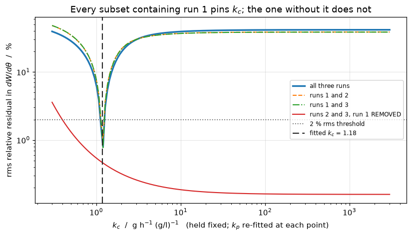

Run 1 is the only run that carries information about $k_c$. Every subset that contains it pins the coefficient to within about 5 %; the subset that does not admits every value above its lower edge, because its profile falls towards the deleted-film fit, which is far inside the threshold. The remaining data are consistent with an infinitely fast liquid film.

That distinction matters and it is easy to blur. $k_c$ is tightly identified: one equation, one unknown, and a narrow band. It is not tested: the narrowness is entirely run 1’s doing, and run 1 is precisely the run Whitman fits $k_c$ to. So the liquid-film coefficient of the two-film theory is, in this paper, determined by one observation and corroborated by none.

That is a quantitative form of the remark the 1962 Foreword quotes from Sherwood and Pigford. It is not a criticism of Whitman, who says the same thing in plainer words across reprint pages 432–433 (the data “are insufficient to prove definitely the truth of the two-film theory”) and calls his own paper “A Preliminary Experimental Confirmation”.

What the data do establish, and it is not nothing: a single film of either kind cannot describe these three runs, by tens of per cent, and a two-film description can. The qualitative claim survives; the quantitative liquid-film coefficient is untested.

6. Where resistance additivity breaks: the textbook formula

The form everyone actually uses is not eq. (4) but its linearised child. With Henry’s law $p = m\,c$, eliminating $p_2 = m\,c_2$ from eq. (4) gives

\[\frac{1}{K_p} = \frac{1}{k_p} + \frac{m}{k_c},\qquad m = \frac{\mathrm{d}p}{\mathrm{d}c},\]

which requires a single $m$. Whitman says this is exactly what fails: “if the deviation from Henry’s law … is considerable, a simplification based on direct proportionality between $p$ and $c$ would be unjustified and the overall coefficients $K_c$ or $K_p$ would have no significance.”

Below, that formula is evaluated with the two most defensible choices of $m$ (the tangent slope at the bulk liquid concentration, and the secant of the reconstructed curve across the run’s own span from $c_3$ to $c_1$) and compared with the exact non-linear interface solve at the same $k_p$, $k_c$. Two checks bracket it. With a linear equilibrium both choices are exact; the break table puts that in. And with the chord from $c_3$ to the solved interface $c_2$ it is exact on the real curve too, an identity, since that chord is what eq. (4) eliminates; but $c_2$ is only known after the solve. So the errors below are the curvature of the equilibrium line between $c_3$ and the point $m$ is taken at.

def additivity_errors(eq, kp=KP_R3, kc=KC_1, runs=RUNS, form="m/k_c"):
    """Error (%) of 1/K_p = 1/k_p + m/k_c per run, with the tangent, the secant
    across c3 to c1 and the chord from c3 to the solved interface c2.
    ``form="1/(m k_c)"`` writes the liquid term upside down (a break row only)."""
    rows = []
    for r in runs:
        p1, c1, c3 = r["p1_mmHg"], r["c1_g_per_l"], r["c3_g_per_l"]
        ex = two_film_algebraic(p1, c3, kp, kc, eq.p)
        K_exact = ex["N"] / (p1 - float(eq.p(c3)))
        m = dict(tangent=float(eq.dpdc(c3)),
                 secant=(float(eq.p(c1)) - float(eq.p(c3))) / (c1 - c3),
                 chord=(ex["p2"] - float(eq.p(c3))) / (ex["c2"] - c3))
        row = dict(run=int(r["run"]), K_p_exact=K_exact)
        for k, v in m.items():
            row[f"m_{k}"] = v
            liquid = v / kc if form == "m/k_c" else 1.0 / (v * kc)
            row[f"err_{k}_pct"] = 100 * (1.0 / (1.0 / kp + liquid) / K_exact - 1)
        rows.append(row)
    return pd.DataFrame(rows)


add = additivity_errors(EQ)
display(add.round(4))
CONSTH_R1_TAN = abs(add.err_tangent_pct.iloc[0])
CONSTH_R1_SEC = abs(add.err_secant_pct.iloc[0])
CONSTH_SEC_MAX = float(np.abs(add.err_secant_pct).max())
CONSTH_TAN_23 = float(np.abs(add.err_tangent_pct.iloc[1:]).max())
CHORD_IDENTITY = float(np.abs(add.err_chord_pct).max()) / 100
EQ_HALF = Equilibrium(EQ.A + 0.5 * EQ.B * np.mean(C_EQ), 0.5 * EQ.B)  # half the slope, same centroid
add_half = additivity_errors(EQ_HALF)
print(f"run 1, the only run with a real liquid resistance: the formula is off by "
      f"{add.err_tangent_pct.iloc[0]:+.1f} % (tangent m) and "
      f"{add.err_secant_pct.iloc[0]:+.1f} % (secant m).")
print(f"worst over all three runs, secant m: {CONSTH_SEC_MAX:.1f} %")
print(f"with the equilibrium slope halved (same centroid) run 1's errors fall to "
      f"{add_half.err_tangent_pct.iloc[0]:+.1f} % and {add_half.err_secant_pct.iloc[0]:+.1f} %")
print(f"runs 2 and 3 are gas-controlled: m/k_c is small against 1/k_p, and the tangent "
      f"is off by at most {CONSTH_TAN_23:.2f} %;")
print("the secant, taken across the large span up to c1, still overestimates m there.")
print(f"with the chord from c3 to the solved interface the formula is exact: below 1e-12 "
      f"(here {CHORD_IDENTITY:.1e})")
print(f"\nThe equilibrium curve rises tenfold every {1 / EQ.B:.1f} g/l; run 1's own "
      f"concentration span is {R[1]['c1_g_per_l'] - R[1]['c3_g_per_l']:g} g/l.")
claims.value("constH_run1_tangent_err_pct", CONSTH_R1_TAN, rtol=1e-3)
claims.value("constH_run1_secant_err_pct", CONSTH_R1_SEC, rtol=1e-3)
claims.value("constH_secant_worst_err_pct", CONSTH_SEC_MAX, rtol=1e-3)
claims.value("constH_runs23_tangent_worst_err_pct", CONSTH_TAN_23, rtol=1e-3)
claims.value("constH_halfslope_run1_tangent_err_pct", abs(add_half.err_tangent_pct.iloc[0]),
             rtol=1e-3)
claims.value("constH_halfslope_run1_secant_err_pct", abs(add_half.err_secant_pct.iloc[0]),
             rtol=1e-3)
claims.bound("constH_interface_chord_identity", CHORD_IDENTITY, max=1e-12, basis="identity",
             note="the chord from c3 to c2 is what eq. (4) eliminates")
claims.value("eq_gl_per_decade", 1 / EQ.B, rtol=1e-3)

	run	K_p_exact	m_tangent	err_tangent_pct	m_secant	err_secant_pct	m_chord	err_chord_pct
0	1	0.2413	1.651	34.1299	3.6208	-12.8179	2.8994	-0.0
1	2	0.5864	0.009	0.1664	0.2472	-10.4197	0.0123	-0.0
2	3	0.5900	0.000	0.0005	0.1138	-5.3631	0.0000	0.0

run 1, the only run with a real liquid resistance: the formula is off by +34.1 % (tangent m) and -12.8 % (secant m).
worst over all three runs, secant m: 12.8 %
with the equilibrium slope halved (same centroid) run 1's errors fall to +14.3 % and +4.9 %
runs 2 and 3 are gas-controlled: m/k_c is small against 1/k_p, and the tangent is off by at most 0.17 %;
the secant, taken across the large span up to c1, still overestimates m there.
with the chord from c3 to the solved interface the formula is exact: below 1e-12 (here 6.7e-16)

The equilibrium curve rises tenfold every 76.9 g/l; run 1's own concentration span is 47 g/l.

7. The overall coefficient is not a property of the apparatus

Same $k_p$, same $k_c$, same equipment. Only the operating point moves, over a window of bulk concentrations and three gas pressures (Whitman’s two and one between). In this window $K_p$ falls and $K_c$ rises monotonically with $c_3$ at every $p_1$ (the steps against that trend are counted below), so the extremes are corners of the window, not samples.

C3_WINDOW = np.linspace(5.0, 415.0, 90)
P1_WINDOW = sorted({P1[1], P1[2], 120.0}, reverse=True)


def overall_coefficients(eq=EQ, kp=KP_R3, kc=KC_1):
    """K_p and K_c over the window, the sampled points where f(c3) < p1."""
    out = {}
    for p1 in P1_WINDOW:
        c3s = C3_WINDOW[eq.p(C3_WINDOW) < p1]
        N = np.array([two_film_algebraic(p1, c, kp, kc, eq.p)["N"] for c in c3s])
        out[p1] = (c3s, N / (p1 - eq.p(c3s)), N / (eq.c(p1) - c3s))
    return out


def range_summary(out):
    kp_all = np.concatenate([v[1] for v in out.values()])
    kc_all = np.concatenate([v[2] for v in out.values()])
    rises = sum(int(np.sum(np.diff(v[1]) > 0)) + int(np.sum(np.diff(v[2]) < 0))
                for v in out.values())
    return kp_all.min(), kp_all.max(), kc_all.min(), kc_all.max(), rises


KOUT = overall_coefficients()
KP_MIN, KP_MAX, KC_MIN, KC_MAX, K_NONMONO = range_summary(KOUT)
fig, axes = plt.subplots(1, 2, figsize=(11.2, 4.2))
for p1, (c3s, Kp, Kc) in KOUT.items():
    axes[0].plot(c3s, Kp, lw=1.8, label=f"$p_1$ = {p1:.0f} mmHg")
    axes[1].plot(c3s, Kc, lw=1.8, label=f"$p_1$ = {p1:.0f} mmHg")
for r in RUNS:
    axes[0].plot(r["c3_g_per_l"], r["K_p"], "ks", ms=7, zorder=5)
    axes[1].plot(r["c3_g_per_l"], r["K_c"], "ks", ms=7, zorder=5)
axes[0].set_ylabel(r"$K_p$  /  g h$^{-1}$ mmHg$^{-1}$")
axes[1].set_ylabel(r"$K_c$  /  g h$^{-1}$ (g/l)$^{-1}$")
for ax in axes:
    ax.set_xlabel(r"bulk liquid concentration $c_3$  /  g l$^{-1}$")
    ax.legend(fontsize=8)
axes[0].set_title("black squares: Whitman's three runs")
fig.suptitle(r"One apparatus, one $k_p$, one $k_c$: the 'overall coefficients' still move",
             y=1.02)
fig.tight_layout()
plt.show()
KP_RANGE_FACTOR, KC_RANGE_FACTOR = KP_MAX / KP_MIN, KC_MAX / KC_MIN
print(f"At fixed k_p = {KP_R3} and k_c = {KC_1:.3f}, over c3 = {C3_WINDOW[0]:g} to "
      f"{C3_WINDOW[-1]:g} g/l and p1 = {P1_WINDOW} mmHg:")
print(f"   K_p ranges over a factor {KP_RANGE_FACTOR:.2f} ({KP_MIN:.4f} to {KP_MAX:.4f})")
print(f"   K_c ranges over a factor {KC_RANGE_FACTOR:.2f} ({KC_MIN:.5f} to {KC_MAX:.5f})")
print(f"   steps against the monotone trend: {K_NONMONO} (the log-linear f is convex, so the")
print("   chord slope from c3 to c2 grows with c3)")
claims.exact("K_window_nonmonotone_steps", K_NONMONO)
claims.value("Kp_range_factor", KP_RANGE_FACTOR, rtol=1e-3)
claims.value("Kc_range_factor", KC_RANGE_FACTOR, rtol=1e-3)
claims.value("Kp_min", KP_MIN, rtol=1e-3)
claims.value("Kp_max", KP_MAX, rtol=1e-4)
claims.value("Kc_min", KC_MIN, rtol=1e-3)
claims.value("Kc_max", KC_MAX, rtol=1e-3)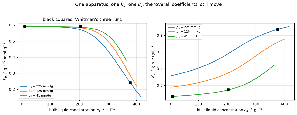

At fixed k_p = 0.59 and k_c = 1.184, over c3 = 5 to 415 g/l and p1 = [225.0, 120.0, 41.0] mmHg:
   K_p ranges over a factor 3.80 (0.1553 to 0.5900)
   K_c ranges over a factor 13.59 (0.06661 to 0.90501)
   steps against the monotone trend: 0 (the log-linear f is convex, so the
   chord slope from c3 to c2 grows with c3)

8. One thing the film model can do that the algebra cannot

The film is a differential object, and writing it as one buys a case the algebra of eq. (4) cannot express: a first-order reaction in the liquid film. The finite-volume solve is checked against the exact film profile (reacting_film_rate in model.py: the hyperbolic-sine profile of a reacting film, closed with the same equilibrium, a scalar root and no grid), first at a moderate rate constant, where the reaction layer is resolved and the scheme’s second order shows, and then at a fast one.

As the rate constant grows the liquid side stops resisting: $c_2 \to 0$ and the rate tends to $k_p\,(p_1 - f(0))$, the gas film alone working against the back pressure of reactant-free liquid. On this page $f(0)$ is not zero: it is the intercept $10^A$ of the reconstructed line, an extrapolation far below the concentrations Table 1 covers. So the remaining gap to $k_p\,p_1$ is set by that intercept, not by the grid: the finite-volume value converges to the exact film value with $n$, and the exact value tends to $f(0)/p_1$ with the rate constant. The break table tests the two candidate causes one at a time.

This is an illustration of the mechanism, not a result about HCl: Whitman publishes no rate constant, and the enhancement regimes belong to F3.1, which owns Hatta’s paper.

KA_MOD, KA_FAST, N_REACT = 10.0, 1e6, 200
N_GASFILM_ONLY = KP_R3 * P1[1]
INTERCEPT_REL = float(EQ.p(0.0)) / P1[1]


def reacting_solve(ka, n, eq=EQ, **kw):
    return TwoFilm(KP_R3, KC_1, eq.p, eq.dpdc, n=n, ka=ka, **kw).solve(P1[1], C3[1])


rows = []
for ka in [0.0, 0.1, 1.0, KA_MOD, 1e3, KA_FAST]:
    s = reacting_solve(ka, N_REACT)
    ex = (two_film_algebraic(P1[1], C3[1], KP_R3, KC_1, EQ.p) if ka == 0 else
          reacting_film_rate(P1[1], C3[1], KP_R3, KC_1, ka, EQ.p, EQ.c))
    rows.append(dict(ka=ka, rate=s["N"], rate_exact_film=ex["N"], c2=s["c2"],
                     c2_exact_film=ex["c2"], one_minus_N_over_kp_p1=1 - s["N"] / N_GASFILM_ONLY))
display(pd.DataFrame(rows))

LADDER = (25, 50, 100)
ex_mod = reacting_film_rate(P1[1], C3[1], KP_R3, KC_1, KA_MOD, EQ.p, EQ.c)
ERR = np.array([abs(reacting_solve(KA_MOD, n)["N"] / ex_mod["N"] - 1) for n in LADDER])
ORDERS = np.log2(ERR[:-1] / ERR[1:])
# round-off of the same solve at the finest rung: the ka = 0 solve is exact there
ROUNDOFF = abs(TwoFilm(KP_R3, KC_1, EQ.p, EQ.dpdc, n=LADDER[-1]).solve(P1[1], C3[1])["N"]
               / two_film_algebraic(P1[1], C3[1], KP_R3, KC_1, EQ.p)["N"] - 1)


def ladder_guard(ref):
    """Finest-rung error against ``ref`` over the round-off of the same grid."""
    err = abs(reacting_solve(KA_MOD, LADDER[-1])["N"] / ref - 1)
    return err / max(ROUNDOFF, np.finfo(float).eps)


GUARD = ladder_guard(ex_mod["N"])
ERR_N200 = abs(reacting_solve(KA_MOD, N_REACT)["N"] / ex_mod["N"] - 1)
print(f"ka = {KA_MOD:g} (reaction layer resolved), rate against the exact film:")
for n, e in zip(LADDER, ERR):
    print(f"   n = {n:4d}   relative error {e:.3e}")
print(f"   observed orders {np.round(ORDERS, 3)}; finest error over the round-off of the "
      f"same grid at least 1e3 (here {GUARD:.0e})")
print(f"   at n = {N_REACT}: {ERR_N200:.2e}")
claims.value("reaction_vs_exact_film_n200", ERR_N200, rtol=0.05)
claims.bound("reaction_order_ka10", ORDERS[-1], min=1.9, max=2.1, basis="theory",
             note="second-order finite volumes, resolved reaction layer")
claims.bound("reaction_ladder_finest_over_roundoff", GUARD, min=1e3, basis="theory",
             note="finest-rung error over the round-off of the same grid (ka = 0 solve)")

ex_fast = reacting_film_rate(P1[1], C3[1], KP_R3, KC_1, KA_FAST, EQ.p, EQ.c)
FAST = {n: reacting_solve(KA_FAST, n) for n in (25, 50, 100, 200, 400, 800, 1600)}
REACTION_LIMIT_RELDEV = 1 - FAST[N_REACT]["N"] / N_GASFILM_ONLY
FAST_EXACT_RESID = 1 - ex_fast["N"] / N_GASFILM_ONLY
print(f"\nka = {KA_FAST:g}: reaction layer sqrt(k_c/ka) = {np.sqrt(KC_1 / KA_FAST):.1e} "
      "of the film")
print(f"   {'n':>5} {'1 - N/(k_p p1)':>15} {'c2 (g/l)':>10}")
for n, s in FAST.items():
    print(f"   {n:5d} {1 - s['N'] / N_GASFILM_ONLY:15.4e} {s['c2']:10.4f}")
print(f"   exact film {FAST_EXACT_RESID:11.4e} {ex_fast['c2']:10.4f}")
print(f"   f(0)/p1 = 10^A/p1 = {INTERCEPT_REL:.4e}: the limit as ka -> infinity")
print(f"\nThe residual converges with n to the exact film value; c2 at n = {N_REACT} is "
      f"{FAST[N_REACT]['c2'] / ex_fast['c2']:.2f} times the exact one, at n = 1600 "
      f"{FAST[1600]['c2'] / ex_fast['c2']:.3f} times,")
print("but c2 is far below the line's scale 1/B, so the rate barely sees it.")
claims.value("reaction_limit_reldev", REACTION_LIMIT_RELDEV, rtol=1e-3)
claims.value("reaction_fast_exact_film_resid", FAST_EXACT_RESID, rtol=1e-4)
claims.value("intercept_over_p1", INTERCEPT_REL, rtol=1e-3)
claims.value("fast_c2_n200_over_exact", FAST[N_REACT]["c2"] / ex_fast["c2"], rtol=1e-3)
claims.value("fast_c2_n1600_over_exact", FAST[1600]["c2"] / ex_fast["c2"], rtol=1e-4)

	ka	rate	rate_exact_film	c2	c2_exact_film	one_minus_N_over_kp_p1
0	0.0	41.000000	41.000000	412.627200	412.627200	0.691149
1	0.1	54.466668	54.466667	407.328738	407.328738	0.589705
2	1.0	121.878611	121.878640	341.430407	341.430317	0.081894
3	10.0	132.745741	132.745741	79.568367	79.567332	0.000032
4	1000.0	132.749559	132.749559	3.858590	3.857890	0.000003
5	1000000.0	132.749605	132.749606	0.238653	0.121997	0.000003

ka = 10 (reaction layer resolved), rate against the exact film:
   n =   25   relative error 6.338e-08
   n =   50   relative error 1.590e-08
   n =  100   relative error 3.978e-09
   observed orders [1.995 1.998]; finest error over the round-off of the same grid at least 1e3 (here 2e+05)
   at n = 200: 9.94e-10

ka = 1e+06: reaction layer sqrt(k_c/ka) = 1.1e-03 of the film
       n  1 - N/(k_p p1)   c2 (g/l)
      25      3.1112e-06     1.6855
      50      3.0341e-06     0.8483
     100      2.9968e-06     0.4352
     200      2.9792e-06     0.2387
     400      2.9718e-06     0.1557
     800      2.9694e-06     0.1290
    1600      2.9689e-06     0.1231
   exact film  2.9688e-06     0.1220
   f(0)/p1 = 10^A/p1 = 2.9580e-06: the limit as ka -> infinity

The residual converges with n to the exact film value; c2 at n = 200 is 1.96 times the exact one, at n = 1600 1.009 times,
but c2 is far below the line's scale 1/B, so the rate barely sees it.

Validation

Checks, ranked by what they can detect, followed by the table that says so.

Equilibrium consistency of Table 1: four printed $(c,p)$ pairs, one two-parameter form, two degrees of freedom. Can fail: a single mis-read digit in any of eight table cells moves it. Corroborated by Table 1’s own duplication of $c_1$ at the shared $p_1$, which involves no fit at all.
Whitman’s worked example, held out: his printed numbers reproduced from Table 1 alone. Can fail: it depends on the reconstruction, on eqs. (4) and (7), and on the $K_p(\text{run 3}) = k_p$ assumption.
The three-run model comparison: one degree of freedom on the two-film fit. Can fail, and it does not pass: the one testable combination is off by about 1 %, three times what a one-parameter model achieves on it. Section 3 states which part of the two-film rms was not free to fail.
The headline computed twice: the deleted-liquid-film rate from the closed form and from a Richardson extrapolation of the root solve at finite $k_c$. The two share the gas-side expression and no solver.
The reacting film against its exact profile: a genuine discretisation error, second order on a resolved layer, with the finest error well above round-off.
pymrm against the algebra, and grid independence: identities (port checks). A linear profile is exact in a conservative finite-volume scheme, so both test the assembly and nothing else. They do move for a wrong geometry index and for a missing equilibrium jump.

What the break table below cannot do

Every row in it perturbs an input and checks that a number moves. That establishes sensitivity, and sensitivity is not correctness: a row proves a claim would notice this defect, and says nothing about whether the undefected value is right. A baseline that is wrong rather than insensitive passes every row it has. That is why the headline has a second route (check 4), the reacting film an exact reference (check 5), and why section 2 shows the liquid-side reading of eq. (4) exceeding its own limit, a defect no perturbation would have found.

The break table

Each row re-runs the affected computation with one thing deliberately wrong, injected through the data, an argument or the equilibrium relation, and hands the result to claims.breaks, which records whether that claim’s own check fails. Three kinds appear: transcription defects (the mid-dot decimal trap this file’s own OCR falls into, digit transpositions), model defects (a wrong nu, the equilibrium jump removed, the Jacobian without the equilibrium slope, an unconverged Newton solve, a linear equilibrium, the intercept of the line removed) and data defects (a rate replaced by one that a single-film model would fit). Rows that do not fail their claim are kept and printed: a blind spot left unstated is an implicit claim.

def rec(t):
    """Table 1 by run number, for a defected copy."""
    return {int(r["run"]): r for r in t.to_dict("records")}


# ---- 1. transcription defects in Table 1
T_DP = t1.copy()
T_DP.loc[T_DP.run == 1, "delta_p_mmHg"] = 107.0                    # 170 transposed
brk("delta_p(run 1) 170 -> 107 (transposed)", "table1_diff_columns_max_dev",
    table1_consistency(T_DP)[0])
T_KC3 = t1.copy()
T_KC3.loc[T_KC3.run == 3, "K_c"] = 0.67                            # 0.067, lost mid-dot
brk("K_c(run 3) 0.067 -> 0.67 (lost mid-dot)", "table1_coef_columns_max_pct",
    table1_consistency(T_KC3)[1])
_r = stated_ratios(T_KC3)
brk("K_c(run 3) 0.067 -> 0.67 (lost mid-dot)", "prose_twelvefold_recomputed", _r[1])
brk("K_c(run 3) 0.067 -> 0.67 (lost mid-dot)", "prose_twofold_recomputed", _r[2])
T_KP1 = t1.copy()
T_KP1.loc[T_KP1.run == 1, "K_p"] = 0.42                            # 0.24 transposed
brk("K_p(run 1) 0.24 -> 0.42 (transposed)", "prose_Kp_ratio_recomputed", stated_ratios(T_KP1)[0])
T_C13 = t1.copy()
T_C13.loc[T_C13.run == 3, "c1_g_per_l"] = 386.0                    # 368 transposed
brk("c1(run 3) 368 -> 386 (transposed)", "c1_distinct_at_shared_p1",
    len(c1_values_at_shared_p1(T_C13)[1]))
brk("c1(run 3) 368 -> 386 (transposed)", "eq_curve_worst_resid_pct",
    Equilibrium.fit(*equilibrium_pairs(T_C13).T).residuals(*equilibrium_pairs(T_C13).T)[0])

# the mid-dot trap on the equilibrium pairs: p3(run 1) 55 read as 5.5
T_P31 = t1.copy()
T_P31.loc[T_P31.run == 1, "p3_mmHg"] = 5.5
_pairs = equilibrium_pairs(T_P31)
EQ_P31 = Equilibrium.fit(*_pairs.T)
_w = EQ_P31.residuals(*_pairs.T)
brk("p3(run 1) 55 -> 5.5 (lost mid-dot)", "eq_curve_worst_resid_pct", _w[0])
brk("p3(run 1) 55 -> 5.5 (lost mid-dot)", "eq_curve_worst_resid_gl", _w[1])
brk("p3(run 1) 55 -> 5.5 (lost mid-dot)", "fig3_axis_top_dev_log10", axis_box(EQ_P31)[2])
brk("p3(run 1) 55 -> 5.5 (lost mid-dot)", "intercept_over_p1", float(EQ_P31.p(0.0)) / P1[1])
for k, v in worked_chain(EQ_P31)[0].items():
    if k != "worked_p2_run1_dev_mmHg":
        brk("p3(run 1) 55 -> 5.5, curve refitted", k, v)
T_P32 = t1.copy()
T_P32.loc[T_P32.run == 2, "p3_mmHg"] = 3.0                         # 0.3 read as 3.0
EQ_P32 = Equilibrium.fit(*equilibrium_pairs(T_P32).T)
brk("p3(run 2) 0.3 -> 3.0 (lost mid-dot)", "eq_pairs_decades",
    np.log10(equilibrium_pairs(T_P32)[:, 1].max() / equilibrium_pairs(T_P32)[:, 1].min()))
brk("p3(run 2) 0.3 -> 3.0 (lost mid-dot)", "negligible_backpressure_mmHg",
    float(EQ_P32.p(C_NEG)))
_rat = dof_ratios(runs=rec(T_P32))
T_DP2 = t1.copy()
T_DP2.loc[T_DP2.run == 2, "delta_p_mmHg"] = 47.0                   # 40.7 misread
_R = rec(T_DP2)
_kpcol = {run: _R[run]["dW_dtheta_g_per_h"] / _R[run]["delta_p_mmHg"] for run in (2, 3)}
_rd = dof_ratios(runs=_R)
brk("delta_p(run 2) 40.7 -> 47.0 (misread)", "kp_disagreement_is_gasfilm_dof",
    abs((_rd["gas"] / _rd["observed"] - 1) - (_kpcol[2] / _kpcol[3] - 1)))
brk("p3(run 2) 0.3 -> 3.0 (lost mid-dot)", "gasfilm_dof_ratio_dev_pct",
    100 * (_rat["gas"] / _rat["observed"] - 1))
brk("p3(run 2) 0.3 -> 3.0 (lost mid-dot)", "ratio_gasfilm_run3_over_run2", _rat["gas"])

# ---- 2. the printed rounding of k_p
KP_UNR = OBS[3] / float(R[3]["delta_p_mmHg"])                      # K_p(run 3) unrounded
brk("k_p taken unrounded, not the printed K_p(run 3)", "worked_p2_run1_dev_mmHg",
    worked_chain(EQ, kp=KP_UNR)[0]["worked_p2_run1_dev_mmHg"])
brk("k_p taken unrounded, not the printed K_p(run 3)", "run2_rate_reldev_no_liquid_film",
    abs(no_liquid_film_rate(P1[2], C3[2], KP_UNR, EQ.p)["N"] / OBS[2] - 1))
_k = range_summary(overall_coefficients(kp=KP_UNR))
brk("k_p taken unrounded, not the printed K_p(run 3)", "Kp_max", _k[1])

# ---- 3. pymrm model defects
for lab, kw in [("construct_div nu = 1 instead of 0", dict(nu=1)),
                ("interface equilibrium removed (p2 = c2)", dict(jump=False))]:
    t = TwoFilm(KP_R3, KC_1, EQ.p, EQ.dpdc, n=40, **kw)
    brk(lab, "pymrm_vs_algebra_reldev",
        abs(t.solve(P1[1], C3[1])["N"] / t.algebraic(P1[1], C3[1])["N"] - 1))
brk("construct_div nu = 1 instead of 0", "grid_spread_rel_n3_to_n600", grid_spread(nu=1)[1])
brk("construct_div nu = 1 instead of 0", "reaction_vs_exact_film_n200",
    abs(reacting_solve(KA_MOD, N_REACT, nu=1)["N"] / ex_mod["N"] - 1))
brk("interface equilibrium removed (p2 = c2)", "reaction_limit_reldev",
    1 - reacting_solve(KA_FAST, N_REACT, jump=False)["N"] / N_GASFILM_ONLY)
_lff = dict(liquid_flux_factor=2.0)
_sl = TwoFilm(KP_R3, KC_1, EQ.p, EQ.dpdc, n=40, **_lff).solve(P1[1], C3[1])
brk(f"TwoFilm({', '.join(f'{k}={v}' for k, v in _lff.items())}): continuity row wrong",
    "interface_flux_continuity", abs(_sl["N_liquid_face"] / _sl["N_gas_face"] - 1))
_bad = TwoFilm(KP_R3, KC_1, EQ.p, EQ.dpdc, n=40)
_s1 = _bad.solve(P1[1], C3[1], maxfev=1, require_success=False)
brk("newton maxfev = 1 (unconverged)", "newton_worst_backward_error", _s1["backward_error"])
_nj = TwoFilm(KP_R3, KC_1, EQ.p, EQ.dpdc, n=40, exact_jacobian=False)
_snj = _nj.solve(P1[1], C3[1], require_success=False)
brk("Jacobian without the equilibrium slope f'(c2)", "newton_max_iterations",
    _snj["nit"] if _snj["success"] else np.inf)
# reacting_film_rate with c3 = 0 is the exact film with its c3/sinh(Ha) term dropped
_ref_bad = reacting_film_rate(P1[1], 0.0, KP_R3, KC_1, KA_MOD, EQ.p, EQ.c)["N"]
_err_bad = [abs(reacting_solve(KA_MOD, n)["N"] / _ref_bad - 1) for n in LADDER[-2:]]
brk("exact film without its c3/sinh(Ha) term (a wrong reference)", "reaction_order_ka10",
    np.log2(_err_bad[0] / _err_bad[1]))
brk(f"finest rung n = {LADDER[-1]} taken as the reference", "reaction_ladder_finest_over_roundoff",
    ladder_guard(reacting_solve(KA_MOD, LADDER[-1])["N"]))

# ---- 4. the curvature of the equilibrium, and the intercept
for k, v in [("constH_run1_tangent_err_pct", abs(add_half.err_tangent_pct.iloc[0])),
             ("constH_run1_secant_err_pct", abs(add_half.err_secant_pct.iloc[0])),
             ("constH_secant_worst_err_pct", float(np.abs(add_half.err_secant_pct).max())),
             ("constH_runs23_tangent_worst_err_pct",
              float(np.abs(add_half.err_tangent_pct.iloc[1:]).max())),
             ("eq_gl_per_decade", 1 / EQ_HALF.B)]:
    brk("equilibrium slope halved (flatter curve)", k, v)
_k = range_summary(overall_coefficients(eq=EQ_HALF))
for k, v in zip(("Kp_min", "Kc_min", "Kc_max", "Kp_range_factor", "Kc_range_factor"),
                (_k[0], _k[2], _k[3], _k[1] / _k[0], _k[3] / _k[2])):
    brk("equilibrium slope halved (flatter curve)", k, v)
for k, v in zip(("kc_band_low_all_runs", "kc_band_high_all_runs"), kc_band((1, 2, 3), eq=EQ_HALF)):
    brk("equilibrium slope halved (flatter curve)", k, v)
_b = [kc_band(s, eq=EQ_HALF)[:2] for s in WITH_RUN1]
brk("equilibrium slope halved (flatter curve)", "kc_band_low_run1_subsets", min(b[0] for b in _b))
brk("equilibrium slope halved (flatter curve)", "kc_band_high_run1_subsets", max(b[1] for b in _b))
brk("equilibrium slope halved (flatter curve)", "kc_band_low_without_run1",
    kc_band((2, 3), eq=EQ_HALF)[0])


class Henry:
    """A linear equilibrium p = m c through run 1's bulk pair: the formula is exact."""
    m = R[1]["p3_mmHg"] / R[1]["c3_g_per_l"]
    p = staticmethod(lambda c: Henry.m * np.asarray(c, float))
    dpdc = staticmethod(lambda c: Henry.m + 0.0 * np.asarray(c, float))


_lin = additivity_errors(Henry)
brk("liquid term written 1/(m k_c) instead of m/k_c", "constH_interface_chord_identity",
    float(np.abs(additivity_errors(EQ, form="1/(m k_c)").err_chord_pct).max()) / 100)
brk("linear equilibrium (Henry's law)", "constH_halfslope_run1_tangent_err_pct",
    abs(_lin.err_tangent_pct.iloc[0]))
brk("linear equilibrium (Henry's law)", "constH_halfslope_run1_secant_err_pct",
    abs(_lin.err_secant_pct.iloc[0]))
EQ_NO_INTERCEPT_P = lambda c: EQ.p(c) - EQ.p(0.0)                  # noqa: E731
_eq0 = type("NoIntercept", (), dict(p=staticmethod(EQ_NO_INTERCEPT_P), dpdc=staticmethod(EQ.dpdc),
                                    c=staticmethod(lambda p: EQ.c(p + EQ.p(0.0)))))
brk("equilibrium intercept removed, f(c) - f(0)", "reaction_limit_reldev",
    1 - reacting_solve(KA_FAST, N_REACT, eq=_eq0)["N"] / N_GASFILM_ONLY)
brk("equilibrium intercept removed, f(c) - f(0)", "reaction_fast_exact_film_resid",
    1 - reacting_film_rate(P1[1], C3[1], KP_R3, KC_1, KA_FAST, _eq0.p, _eq0.c)["N"]
    / N_GASFILM_ONLY)
brk(f"grid n = {N_REACT} -> 25 (the grid, the other candidate cause)", "reaction_limit_reldev",
    1 - FAST[25]["N"] / N_GASFILM_ONLY)
brk(f"grid n = {N_REACT} -> 25", "fast_c2_n200_over_exact", FAST[25]["c2"] / ex_fast["c2"])
brk("grid n = 1600 -> 800", "fast_c2_n1600_over_exact", FAST[800]["c2"] / ex_fast["c2"])

# ---- 5. the curve without its extreme point
EQ_NO425 = Equilibrium.fit(C_EQ[C_EQ < C_EQ.max()], P_EQ[C_EQ < C_EQ.max()])
brk("curve refitted without its highest pair", "fig3_axis_top_dev_log10", axis_box(EQ_NO425)[2])
for k, v in worked_chain(EQ_NO425)[0].items():
    if k != "worked_p2_run1_dev_mmHg":               # arithmetic on Table 1, no curve in it
        brk("curve refitted without its highest pair", k, v)

# ---- 6. defects in the data that the model comparison must see
RUNS_GASFIT = [dict(r) for r in RUNS]
RUNS_GASFIT[0]["dW_dtheta_g_per_h"] = par_g[0] * (P1[1] - R[1]["p3_mmHg"])
_fg = fit(lambda th: rel_resid_gas(th, runs=RUNS_GASFIT), [np.log(0.4)])
brk("run 1 rate replaced by k_p (p1 - p3)", "gasfilm_3run_rms_pct", 100 * _fg[2])
brk("run 1 rate replaced by k_p (p1 - p3)", "gasfilm_3run_worst_pct", 100 * np.abs(_fg[1]).max())
_f2 = fit(lambda th: rel_resid_two(th, runs=RUNS_GASFIT), np.log([0.59, 1.2]))
brk("run 1 rate replaced by k_p (p1 - p3)", "twofilm_run1_resid_pct", 100 * abs(_f2[1][0]))
RUNS_LIQFIT = [dict(r) for r in RUNS]
for rr in RUNS_LIQFIT:
    rr["dW_dtheta_g_per_h"] = par_l[0] * (rr["c1_g_per_l"] - rr["c3_g_per_l"])
_fl = fit(lambda th: rel_resid_liq(th, runs=RUNS_LIQFIT), [np.log(0.3)])
brk("all rates replaced by k_c (c1 - c3)", "liquidfilm_3run_rms_pct", 100 * _fl[2])
brk("all rates replaced by k_c (c1 - c3)", "liquidfilm_3run_worst_pct", 100 * np.abs(_fl[1]).max())
T_R3 = t1.copy()
T_R3.loc[T_R3.run == 3, "dW_dtheta_g_per_h"] = 24.0                # 24.1, last digit lost
RUNS_R3 = T_R3.to_dict("records")
brk("run 3 rate 24.1 -> 24.0 (last digit lost)", "gasfilm_runs23_rms_pct",
    100 * fit(lambda th: rel_resid_gas(th, runs=RUNS_R3, subset=(2, 3)), [np.log(0.59)])[2])
brk("run 3 rate 24.1 -> 24.0 (last digit lost)", "nolf_runs23_rms_pct",
    100 * fit(lambda th: rel_resid_nolf(th, runs=RUNS_R3, subset=(2, 3)), [np.log(0.59)])[2])
_rat = dof_ratios(runs=rec(T_R3))
brk("run 3 rate 24.1 -> 24.0 (last digit lost)", "ratio_observed_run3_over_run2",
    _rat["observed"])
brk("run 3 rate 24.1 -> 24.0 (last digit lost)", "dof_gap_fraction",
    (_rat["observed"] - 1) / (_rat["two"] - 1))

# ---- 7. the liquid film deleted: which claim notices and which does not
brk("k_c -> infinity (liquid film deleted)", "run2_rate_reldev",
    abs(NO_LF["N"] / OBS[2] - 1))
_fn = fit(rel_resid_nolf, [np.log(0.59)])
brk("k_c -> infinity (liquid film deleted)", "twofilm_3run_rms_pct", 100 * _fn[2])
brk("k_c -> infinity (liquid film deleted)", "twofilm_3run_worst_pct", 100 * np.abs(_fn[1]).max())
brk("k_c -> infinity (liquid film deleted)", "twofilm_runs23_rms_pct",
    100 * fit(lambda th: rel_resid_nolf(th, subset=(2, 3)), [np.log(0.59)])[2])
brk("k_c -> infinity (liquid film deleted)", "twofilm_fit_run2_p2_mmHg",
    no_liquid_film_rate(P1[2], C3[2], KP_F, EQ.p)["p2"])
brk("k_c -> infinity (liquid film deleted)", "dof_ratio_overpredict_pct",
    100 * (RAT["nolf"] / RAT["observed"] - 1))
brk("k_c -> infinity (liquid film deleted)", "ratio_twofilm_run3_over_run2", RAT["nolf"])
brk("k_c -> infinity (liquid film deleted)", "dof_gap_fraction",
    (RAT["observed"] - 1) / (RAT["nolf"] - 1))
brk("k_c -> infinity (liquid film deleted)", "run2_liquid_film_effect", 0.0)
for run, name in ((2, "run2_gasfilm_resistance_share"), (1, "run1_gasfilm_resistance_share")):
    brk("k_c / 8", name, resistance_share(EQ, KC_1 / 8, run))
brk("route B without the Richardson step", "no_liquid_film_two_routes",
    abs(route_b(K_A, extrapolate=False) / NO_LF["N"] - 1))
brk("run 1 removed from the fit", "kc_band_width_all_runs",
    BANDS[(2, 3)][1] / BANDS[(2, 3)][0])

for _lab, _mod in (("run 3 rate 24.1 -> 24.3", (3, 24.3)), ("run 2 rate 24.0 -> 42.0", (2, 42.0))):
    _t = t1.copy()
    _t.loc[_t.run == _mod[0], "dW_dtheta_g_per_h"] = _mod[1]
    _lo, _hi, _pr = kc_band((2, 3), runs=_t.to_dict("records"))
    brk(_lab, "profile_without_run1_rises", int(np.sum(np.diff(_pr) > 0)))
    brk(_lab, "kc_band_without_run1_unbounded", bool(np.isinf(_hi)))
_bl, _al = np.polyfit(np.log10(C_EQ), P_EQ, 1)


class LinLog:
    """Equilibrium fitted as p linear in log10 c (Fig. 3's axes swapped): concave."""
    p = staticmethod(lambda c: _al + _bl * np.log10(np.asarray(c, float)))
    c = staticmethod(lambda p: 10 ** ((np.asarray(p, float) - _al) / _bl))
    dpdc = staticmethod(lambda c: _bl / (np.asarray(c, float) * np.log(10.0)))


brk("equilibrium fitted as p linear in log10 c (axes swapped)", "K_window_nonmonotone_steps",
    range_summary(overall_coefficients(eq=LinLog))[4])

# ---- 8. the back pressure removed altogether: the one degree of freedom
PQ0 = Equilibrium(-300.0, 0.0)                                     # p = 1e-300, no back pressure
_rat0 = dof_ratios(eq=PQ0)
brk("equilibrium back pressure set to zero", "ratio_nolf_run3_over_run2", _rat0["nolf"])

True

# The break table, as recorded by claims.breaks.
print(f"{'injected defect':<56} {'claim':<38} {'clean':>11} {'broken':>11}  caught")
for name, metric, clean, broken, caught in BREAK:
    is_bound = claims.metrics[metric]["kind"] == "bound"
    shown = f"(here {clean:.1e})" if is_bound else f"{clean:11.4g}"
    print(f"{name[:56]:<56} {metric[:38]:<38} {shown:>11} {broken:11.4g}  "
          f"{'yes' if caught else 'NO'}")
_caught = {m for _, m, _, _, c in BREAK if c}
_structural = sorted(k for k, c in claims.metrics.items() if c.get("structural"))
_open = sorted(k for k in claims.metrics if k not in _caught and k not in _structural)
print(f"\n{len(BREAK)} rows; {len(_caught)} of {len(claims.metrics)} claims are failed by at "
      f"least one row; structural: {', '.join(_structural) or 'none'}; "
      f"open: {', '.join(_open) or 'none'}")
_uncaught = [(n, m) for n, m, _, _, c in BREAK if not c]
print("rows that do not fail their claim: "
      + (", ".join(f"{n} -> {m}" for n, m in _uncaught) or "none"))

injected defect                                          claim                                        clean      broken  caught
delta_p(run 1) 170 -> 107 (transposed)                   table1_diff_columns_max_dev            (here 0.0e+00)          63  yes
K_c(run 3) 0.067 -> 0.67 (lost mid-dot)                  table1_coef_columns_max_pct                 0.4902       89.98  yes
K_c(run 3) 0.067 -> 0.67 (lost mid-dot)                  prose_twelvefold_recomputed                  12.99       1.299  yes
K_c(run 3) 0.067 -> 0.67 (lost mid-dot)                  prose_twofold_recomputed                     2.179      0.2179  yes
K_p(run 1) 0.24 -> 0.42 (transposed)                     prose_Kp_ratio_recomputed                    2.458       1.405  yes
c1(run 3) 368 -> 386 (transposed)                        c1_distinct_at_shared_p1                         1           2  yes
c1(run 3) 368 -> 386 (transposed)                        eq_curve_worst_resid_pct                    0.3833       33.47  yes
p3(run 1) 55 -> 5.5 (lost mid-dot)                       eq_curve_worst_resid_pct                    0.3833       123.5  yes
p3(run 1) 55 -> 5.5 (lost mid-dot)                       eq_curve_worst_resid_gl                     0.1277       60.16  yes
p3(run 1) 55 -> 5.5 (lost mid-dot)                       fig3_axis_top_dev_log10                   0.008108      0.3846  yes
p3(run 1) 55 -> 5.5 (lost mid-dot)                       intercept_over_p1                        2.958e-06   4.396e-06  yes
p3(run 1) 55 -> 5.5, curve refitted                      worked_c2_run1_dev_gl                       0.6272       29.02  yes
p3(run 1) 55 -> 5.5, curve refitted                      worked_kc_reldev                            0.0133      0.4579  yes
p3(run 1) 55 -> 5.5, curve refitted                      run2_c2_dev_gl                              0.1565       16.57  yes
p3(run 1) 55 -> 5.5, curve refitted                      run2_p2_dev_mmHg                           0.05095     0.07588  yes
p3(run 1) 55 -> 5.5, curve refitted                      run2_rate_reldev                          0.005581    0.008699  yes
p3(run 2) 0.3 -> 3.0 (lost mid-dot)                      eq_pairs_decades                             2.875       1.875  yes
p3(run 2) 0.3 -> 3.0 (lost mid-dot)                      negligible_backpressure_mmHg                 1.191       6.246  yes
delta_p(run 2) 40.7 -> 47.0 (misread)                    kp_disagreement_is_gasfilm_dof         (here 2.2e-16)      0.1345  yes
p3(run 2) 0.3 -> 3.0 (lost mid-dot)                      gasfilm_dof_ratio_dev_pct                   0.3191       7.447  yes
p3(run 2) 0.3 -> 3.0 (lost mid-dot)                      ratio_gasfilm_run3_over_run2                 1.007       1.079  yes
k_p taken unrounded, not the printed K_p(run 3)          worked_p2_run1_dev_mmHg                     0.4915       0.751  yes
k_p taken unrounded, not the printed K_p(run 3)          run2_rate_reldev_no_liquid_film          0.0005375    0.003185  yes
k_p taken unrounded, not the printed K_p(run 3)          Kp_max                                        0.59      0.5878  yes
construct_div nu = 1 instead of 0                        pymrm_vs_algebra_reldev                (here 1.8e-13)           1  yes
interface equilibrium removed (p2 = c2)                  pymrm_vs_algebra_reldev                (here 1.8e-13)       2.469  yes
construct_div nu = 1 instead of 0                        grid_spread_rel_n3_to_n600             (here 5.9e-11)       4.016  yes
construct_div nu = 1 instead of 0                        reaction_vs_exact_film_n200              9.945e-10           1  yes
interface equilibrium removed (p2 = c2)                  reaction_limit_reldev                    2.979e-06     0.00106  yes
TwoFilm(liquid_flux_factor=2.0): continuity row wrong    interface_flux_continuity              (here 1.3e-13)         0.5  yes
newton maxfev = 1 (unconverged)                          newton_worst_backward_error            (here 1.5e-16)     0.01619  yes
Jacobian without the equilibrium slope f'(c2)            newton_max_iterations                  (here 6.0e+00)         inf  yes
exact film without its c3/sinh(Ha) term (a wrong referen reaction_order_ka10                    (here 2.0e+00)   0.0007555  yes
finest rung n = 100 taken as the reference               reaction_ladder_finest_over_roundoff   (here 2.1e+05)           0  yes
equilibrium slope halved (flatter curve)                 constH_run1_tangent_err_pct                  34.13       14.31  yes
equilibrium slope halved (flatter curve)                 constH_run1_secant_err_pct                   12.82       4.949  yes
equilibrium slope halved (flatter curve)                 constH_secant_worst_err_pct                  12.82       5.367  yes
equilibrium slope halved (flatter curve)                 constH_runs23_tangent_worst_err_pct         0.1664       0.277  yes
equilibrium slope halved (flatter curve)                 eq_gl_per_decade                             76.86       153.7  yes
equilibrium slope halved (flatter curve)                 Kp_min                                      0.1553      0.3592  yes
equilibrium slope halved (flatter curve)                 Kc_min                                     0.06661     0.06217  yes
equilibrium slope halved (flatter curve)                 Kc_max                                       0.905      0.6603  yes
equilibrium slope halved (flatter curve)                 Kp_range_factor                              3.799       1.641  yes
equilibrium slope halved (flatter curve)                 Kc_range_factor                              13.59       10.62  yes
equilibrium slope halved (flatter curve)                 kc_band_low_all_runs                         1.126         nan  yes
equilibrium slope halved (flatter curve)                 kc_band_high_all_runs                        1.244         nan  yes
equilibrium slope halved (flatter curve)                 kc_band_low_run1_subsets                     1.126         nan  yes
equilibrium slope halved (flatter curve)                 kc_band_high_run1_subsets                    1.244         nan  yes
equilibrium slope halved (flatter curve)                 kc_band_low_without_run1                    0.3959         nan  yes
liquid term written 1/(m k_c) instead of m/k_c           constH_interface_chord_identity        (here 6.7e-16)       1.086  yes
linear equilibrium (Henry's law)                         constH_halfslope_run1_tangent_err_pct        14.31    2.22e-14  yes
linear equilibrium (Henry's law)                         constH_halfslope_run1_secant_err_pct         4.949    2.22e-14  yes
equilibrium intercept removed, f(c) - f(0)               reaction_limit_reldev                    2.979e-06   2.122e-08  yes
equilibrium intercept removed, f(c) - f(0)               reaction_fast_exact_film_resid           2.969e-06   1.083e-08  yes
grid n = 200 -> 25 (the grid, the other candidate cause) reaction_limit_reldev                    2.979e-06   3.111e-06  yes
grid n = 200 -> 25                                       fast_c2_n200_over_exact                      1.956       13.82  yes
grid n = 1600 -> 800                                     fast_c2_n1600_over_exact                     1.009       1.058  yes
curve refitted without its highest pair                  fig3_axis_top_dev_log10                   0.008108    0.008739  yes
curve refitted without its highest pair                  worked_c2_run1_dev_gl                       0.6272      0.5901  yes
curve refitted without its highest pair                  worked_kc_reldev                            0.0133     0.01224  yes
curve refitted without its highest pair                  run2_c2_dev_gl                              0.1565      0.1351  yes
curve refitted without its highest pair                  run2_p2_dev_mmHg                           0.05095     0.05143  NO
curve refitted without its highest pair                  run2_rate_reldev                          0.005581    0.005569  NO
run 1 rate replaced by k_p (p1 - p3)                     gasfilm_3run_rms_pct                         41.71       28.33  yes
run 1 rate replaced by k_p (p1 - p3)                     gasfilm_3run_worst_pct                       44.29        30.4  yes
run 1 rate replaced by k_p (p1 - p3)                     twofilm_run1_resid_pct                    0.005428    0.002338  yes
all rates replaced by k_c (c1 - c3)                      liquidfilm_3run_rms_pct                      59.47   4.045e-08  yes
all rates replaced by k_c (c1 - c3)                      liquidfilm_3run_worst_pct                    90.28   4.045e-08  yes
run 3 rate 24.1 -> 24.0 (last digit lost)                gasfilm_runs23_rms_pct                      0.1593      0.3672  yes
run 3 rate 24.1 -> 24.0 (last digit lost)                nolf_runs23_rms_pct                         0.1584      0.3663  yes
run 3 rate 24.1 -> 24.0 (last digit lost)                ratio_observed_run3_over_run2                1.004           1  yes
run 3 rate 24.1 -> 24.0 (last digit lost)                dof_gap_fraction                            0.3076           0  yes
k_c -> infinity (liquid film deleted)                    run2_rate_reldev                          0.005581   0.0005375  yes
k_c -> infinity (liquid film deleted)                    twofilm_3run_rms_pct                        0.3795       41.68  yes
k_c -> infinity (liquid film deleted)                    twofilm_3run_worst_pct                      0.4696       44.26  yes
k_c -> infinity (liquid film deleted)                    twofilm_runs23_rms_pct                      0.4647      0.1584  yes
k_c -> infinity (liquid film deleted)                    twofilm_fit_run2_p2_mmHg                    0.5495      0.3002  yes
k_c -> infinity (liquid film deleted)                    dof_ratio_overpredict_pct                   0.9338      0.3174  yes
k_c -> infinity (liquid film deleted)                    ratio_twofilm_run3_over_run2                 1.014       1.007  yes
k_c -> infinity (liquid film deleted)                    dof_gap_fraction                            0.3076      0.5666  yes
k_c -> infinity (liquid film deleted)                    run2_liquid_film_effect                   0.006153           0  yes
k_c / 8                                                  run2_gasfilm_resistance_share               0.9939      0.7393  yes
k_c / 8                                                  run1_gasfilm_resistance_share                0.409     0.06679  yes
route B without the Richardson step                      no_liquid_film_two_routes              (here 1.3e-12)   4.481e-08  yes
run 1 removed from the fit                               kc_band_width_all_runs                       1.105         inf  yes
run 3 rate 24.1 -> 24.3                                  profile_without_run1_rises                       0         133  yes
run 3 rate 24.1 -> 24.3                                  kc_band_without_run1_unbounded                   1           1  NO
run 2 rate 24.0 -> 42.0                                  profile_without_run1_rises                       0           0  NO
run 2 rate 24.0 -> 42.0                                  kc_band_without_run1_unbounded                   1           0  yes
equilibrium fitted as p linear in log10 c (axes swapped) K_window_nonmonotone_steps                       0         466  yes
equilibrium back pressure set to zero                    ratio_nolf_run3_over_run2                    1.007           1  yes

91 rows; 77 of 78 claims are failed by at least one row; structural: fig3_axis_bottom_identity; open: none
rows that do not fail their claim: curve refitted without its highest pair -> run2_p2_dev_mmHg, curve refitted without its highest pair -> run2_rate_reldev, run 3 rate 24.1 -> 24.3 -> kc_band_without_run1_unbounded, run 2 rate 24.0 -> 42.0 -> profile_without_run1_rises

What pymrm adds

Not the two-film answer itself. For Whitman’s problem the pymrm solve reproduces the algebra to round-off by construction, and the page says so rather than presenting it as validation. A resistance-in-series identity does not need a solver.

What it adds is three things the 1923 paper could not do.

Two results on this page need no pymrm at all, and the page says so:

The interface state, solved instead of read off a chart. Steps 3 and 5 of the worked example are Whitman finding a point on Fig. 3 by eye. Closing eq. (4) with $p_2 = f(c_2)$ makes that a scalar root (two_film_algebraic, brentq), which is why sections 6 and 7 can put his three hand-worked points inside a continuous sweep of the operating plane: at fixed $k_p$ and $k_c$ the “overall coefficients” move by the factors printed there, properties of the operating point and not of the apparatus. The pymrm solve gives the same interface (the port check) but is not needed for it.
A number on how badly the linearised form fails (section 6), against the same scalar root.

What pymrm contributes is the film as a coupled finite-volume object:

Section 8 puts a reaction in the liquid film and checks the finite-volume solve against the exact reacting-film profile at second order. For first-order kinetics that profile exists in closed form, so the check is the point here: the same TwoFilm, with no change but the source, is what carries over to kinetics, geometries and property variations that have no closed form.
The coupling pattern: two films on one BlockLayout, their interface values as shapes_d unknowns, every block placed by name, and the one nonlinear row with an exact derivative; it converges in a few Newton iterations from the deleted-film state and fails without that derivative.

And one thing that is not pymrm at all. The most useful output of this page is the power analysis of sections 2 and 5: Whitman’s single held-out prediction is almost entirely gas-film controlled, and removing run 1 leaves $k_c$ unbounded above. That needed a careful reading of Table 1 and no solver. It is included because it is the answer to the question the 1962 Foreword raises, and because a page about a resistance-in-series identity that reported only identities would be worthless.

Reuse

The pattern to lift is TwoFilm in model.py: two domains, each with its own construct_grad/construct_div pair, coupled by (i) flux continuity and (ii) a non-linear jump condition between the two field variables at the shared face, with both interface values carried as external unknowns through shapes_d so the operators stay constant, and all of it placed on one BlockLayout. Any partition-equilibrium interface has this shape: gas/liquid, membrane/feed, solid/fluid at an adsorption isotherm. Where the jump is linear (a constant partition coefficient), pymrm.construct_interface_matrices eliminates the interface values instead.

Read interface fluxes from the faces. The absorption rate here is the gas-film flux at the interface face from compute_boundary_values; the implementation cell checks it against the liquid-side face flux.

Numbers you may take from this page, and the ones you may not.

$k_p$ and $k_c$ are per-apparatus conductances for one 1923 rig, not film coefficients. They carry no area and no thickness. They are not transferable to anything.
The reconstructed equilibrium relation $\log_{10}(p/\mathrm{mmHg}) = A + B\,c$ is fitted to Whitman’s own four printed points at 30 °C and is a reconstruction of the curve he drew, not a thermodynamic correlation for HCl. Use it inside this page’s argument and nowhere else, and not at all far below the concentrations Table 1 covers: section 8 shows its intercept deciding a limit. Modern HCl vapour-pressure data are better and are not here.
$k_c$ should be treated as fitted, not measured. Section 5 shows it rests entirely on run 1: with all three runs the admitted band is narrow, but remove run 1 and the remaining data admit every value above about 0.4. A tight band around a value that one observation sets by itself is identification, not corroboration. Do not quote Whitman’s printed $k_c$ as a measured liquid-film coefficient.

If you are choosing between film, penetration and surface-renewal theory, this page cannot help: it establishes only that a single film fails on these data and that two films fit them with one degree of freedom to spare. The diffusivity exponent that distinguishes the three pictures is not something Whitman’s data can see. Go to A3.2 instead: it is the page holding all three sources at once, and it takes the three-way comparison on the one measured coefficient available there, with film and surface renewal each fitting that datum by construction and penetration alone predicting it with no free constant. It does not settle the underlying $\sqrt{D}$ exponent (one measured coefficient at one diffusivity cannot resolve an exponent), so that question still stands.

If you need enhancement by reaction, go to F3.1; the reaction cell here is a limit check, not a model. $k_p$ and $k_c$ are also assumed equal across all three runs, which Whitman explicitly says need not hold and which three runs cannot check.

Related: F3.1 (reaction in the liquid film), F3.5 (a modern two-film absorption model with speciation), A2.1 (outward-normal boundary conditions), A4.4 (resistances in series in a different guise, and where that addition is exact), H1.4 (two domains on one BlockLayout).

References

Whitman, W. G. (1923). The two-film theory of gas absorption. Chemical and Metallurgical Engineering 29, 146–148. The origin of the result, cited and not consulted. The 1923 printing is pre-DOI and unreachable; the volume and page range are the ones printed in the 1962 reprint’s own header and are inherited, not verified. No issue number is given, because the reprint’s header does not print one and the 1923 printing was not seen.

Whitman, W. G. (1962). The two-film theory of gas absorption. In Pioneer papers in convective mass transfer, 5. International Journal of Heat and Mass Transfer 5(5), 429–433. doi:10.1016/0017-9310(62)90032-7. The text actually read. A verbatim reprint of the 1923 article, with an Editor’s Foreword. Eqs. (1) to (8), Table 1, the worked example and the printed axis labels of Figs 2 and 3 were all transcribed from renders of this printing at its native 300 ppi, each numeric cropped and re-read at that resolution, and every page reference on this page is to it.

Sherwood, T. K. and Pigford, R. L. (1951). Absorption and Extraction. McGraw-Hill. Quoted through the 1962 Editor’s Foreword, which gives it as “their book Absorption and Extraction (McGraw-Hill, 1951)” and reproduces the sentence used here. No edition is stated there and none is asserted here; the book itself is not on disk.

Whitman, W. G. and Keats, J. L. (1922). J. Ind. Eng. Chem. 14, 185. Whitman’s own earlier humidification and dehumidification work, cited by him as the source of the two-film picture. Not consulted.

Dolezalek, F. (1898). Z. phys. Chem. 26, 334, and Bates, S. J. and Kirschman, H. D. (1919). J. Am. Chem. Soc. 41, 1897: the HCl vapour-pressure data plotted as crosses and circles on Whitman’s Fig. 3. Not consulted, and not digitised: the equilibrium relation used here is reconstructed from Whitman’s own Table 1.

# Claims: every registered number printed, agreement.json written for CI, and an
# exception raised when a claim fails its own check or has no break row.
for _lit, _name in (("99.4 %", "run2_gasfilm_resistance_share"),
                    ("0.6 %", "run2_liquid_film_effect"),
                    ("0.4", "kc_band_low_without_run1")):
    claims.says(_lit, _name)
claims.report();   # the semicolon keeps the notebook from echoing the payload

Claims for A3.1:
  table1_diff_columns_max_dev           = (here 0.0e+00)   bound  bound <= 1e-09 [identity]
  table1_coef_columns_max_pct           = 0.4902           value  rtol 0.01
  prose_Kp_ratio_recomputed             = 2.4583           value  rtol 0.001
  prose_twelvefold_recomputed           = 12.985           value  rtol 0.001
  prose_twofold_recomputed              = 2.1791           value  rtol 0.001
  c1_distinct_at_shared_p1              = 1                exact  exact
  eq_curve_worst_resid_pct              = 0.3833           value  rtol 0.01
  eq_curve_worst_resid_gl               = 0.1277           value  rtol 0.01
  eq_pairs_decades                      = 2.8751           value  rtol 0.001
  fig3_axis_top_dev_log10               = 0.008108         value  rtol 0.01
  fig3_axis_bottom_identity             = (here 0.0e+00)   bound  bound <= 1e-12 [identity]
  negligible_backpressure_mmHg          = 1.1909           value  rtol 0.01
  pymrm_vs_algebra_reldev               = (here 1.8e-13)   bound  bound <= 1e-11 [identity]
  newton_worst_backward_error           = (here 1.5e-16)   bound  bound <= 1e-12 [tolerance]
  newton_max_iterations                 = (here 6.0e+00)   bound  bound <= 10 [chosen]
  interface_flux_continuity             = (here 1.3e-13)   bound  bound <= 1e-10 [identity]
  grid_spread_rel_n3_to_n600            = (here 5.9e-11)   bound  bound <= 1e-09 [identity]
  worked_p2_run1_dev_mmHg               = 0.49153          value  rtol 0.01
  worked_c2_run1_dev_gl                 = 0.6272           value  rtol 0.01
  worked_kc_reldev                      = 0.0133           value  rtol 0.01
  run2_c2_dev_gl                        = 0.15646          value  rtol 0.01
  run2_p2_dev_mmHg                      = 0.050946         value  rtol 0.01
  run2_rate_reldev                      = 0.0055809        value  rtol 0.01
  run2_gasfilm_resistance_share         = 0.99388          value  rtol 0.001
  run1_gasfilm_resistance_share         = 0.40904          value  rtol 0.001
  run2_rate_reldev_no_liquid_film       = 0.00053752       value  rtol 0.01
  run2_liquid_film_effect               = 0.0061528        value  rtol 0.01
  no_liquid_film_two_routes             = (here 1.3e-12)   bound  bound <= 1e-10 [tolerance]
  gasfilm_3run_rms_pct                  = 41.708           value  rtol 0.001
  liquidfilm_3run_rms_pct               = 59.474           value  rtol 0.001
  twofilm_3run_rms_pct                  = 0.37946          value  rtol 0.001
  gasfilm_3run_worst_pct                = 44.289           value  rtol 0.001
  liquidfilm_3run_worst_pct             = 90.284           value  rtol 0.001
  twofilm_3run_worst_pct                = 0.46958          value  rtol 0.001
  twofilm_run1_resid_pct                = 0.0054278        value  rtol 0.05
  gasfilm_runs23_rms_pct                = 0.1593           value  rtol 0.001
  nolf_runs23_rms_pct                   = 0.15844          value  rtol 0.001
  twofilm_runs23_rms_pct                = 0.46473          value  rtol 0.001
  twofilm_fit_run2_p2_mmHg              = 0.54945          value  rtol 0.001
  ratio_observed_run3_over_run2         = 1.0042           value  rtol 1e-05
  ratio_twofilm_run3_over_run2          = 1.0135           value  rtol 1e-05
  ratio_gasfilm_run3_over_run2          = 1.0074           value  rtol 1e-05
  ratio_nolf_run3_over_run2             = 1.0074           value  rtol 1e-05
  dof_ratio_overpredict_pct             = 0.9338           value  rtol 0.001
  gasfilm_dof_ratio_dev_pct             = 0.3191           value  rtol 0.001
  dof_gap_fraction                      = 0.30765          value  rtol 0.001
  kp_disagreement_is_gasfilm_dof        = (here 2.2e-16)   bound  bound <= 1e-12 [identity]
  kc_band_without_run1_unbounded        = True             exact  exact
  profile_without_run1_rises            = 0                exact  exact
  kc_band_low_all_runs                  = 1.1259           value  rtol 0.0001
  kc_band_high_all_runs                 = 1.2439           value  rtol 0.0001
  kc_band_width_all_runs                = 1.1048           value  rtol 0.0001
  kc_band_low_run1_subsets              = 1.1259           value  rtol 0.0001
  kc_band_high_run1_subsets             = 1.2439           value  rtol 0.0001
  kc_band_low_without_run1              = 0.39592          value  rtol 0.0001
  constH_run1_tangent_err_pct           = 34.13            value  rtol 0.001
  constH_run1_secant_err_pct            = 12.818           value  rtol 0.001
  constH_secant_worst_err_pct           = 12.818           value  rtol 0.001
  constH_runs23_tangent_worst_err_pct   = 0.16644          value  rtol 0.001
  constH_halfslope_run1_tangent_err_pct = 14.312           value  rtol 0.001
  constH_halfslope_run1_secant_err_pct  = 4.9491           value  rtol 0.001
  constH_interface_chord_identity       = (here 6.7e-16)   bound  bound <= 1e-12 [identity]
  eq_gl_per_decade                      = 76.86            value  rtol 0.001
  K_window_nonmonotone_steps            = 0                exact  exact
  Kp_range_factor                       = 3.7994           value  rtol 0.001
  Kc_range_factor                       = 13.586           value  rtol 0.001
  Kp_min                                = 0.15528          value  rtol 0.001
  Kp_max                                = 0.58999          value  rtol 0.0001
  Kc_min                                = 0.066613         value  rtol 0.001
  Kc_max                                = 0.90501          value  rtol 0.001
  reaction_vs_exact_film_n200           = 9.945e-10        value  rtol 0.05
  reaction_order_ka10                   = (here 2.0e+00)   bound  bound [1.9, 2.1] [theory]
  reaction_ladder_finest_over_roundoff  = (here 2.1e+05)   bound  bound >= 1000 [theory]
  reaction_limit_reldev                 = 2.9792e-06       value  rtol 0.001
  reaction_fast_exact_film_resid        = 2.9688e-06       value  rtol 0.0001
  intercept_over_p1                     = 2.958e-06        value  rtol 0.001
  fast_c2_n200_over_exact               = 1.9562           value  rtol 0.001
  fast_c2_n1600_over_exact              = 1.0094           value  rtol 0.0001