try:
    import pymrm
except ImportError:
%pip install -q pymrm pyyamlCO2 absorption into amine-promoted carbonate solutions
sec:F
struct:S3
struct:S10
tier:T1
data:tier6
phase:gas-liquid
Seven species, two kinetic reactions and two acid-base equilibria decide how fast CO2 enters hot potash with an amine promoter. This page rebuilds the film model that settled the shuttle-versus-catalysis debate.
CO2 absorption into amine-promoted carbonate solutions
Catalog ID: F3.5 · Structures: S3 (1D steady BVP) + S10 (instantaneous-equilibrium constraints) · Tier: T1
Add 3 mol% of an amine to a hot potassium carbonate solution and CO2 absorbs five times faster. For twenty years the field argued about why — a “shuttle” carrying CO2 into the bulk as carbamate, or homogeneous catalysis of the hydration reaction — using approximate models that each captured one mechanism and excluded the other. Bosch, Versteeg and van Swaaij ended the argument by refusing to approximate: solve the diffusion–reaction film with every reaction in it, reversible, simultaneously, and ask the solution what it is doing.
That model is a seven-species boundary-value problem with two kinetic reactions and two acid–base equilibria — exactly the shape of problem pymrm’s operators are built for. This page reproduces their Table 2 (twelve enhancement factors, twelve fluxes, eight promotion factors), their desorption promotion factor, and their concentration profiles — and in doing so uncovers an inconsistency between the printed equilibrium constants and the ones their code must have used. One rescaled constant, fitted to the paper’s own numbers, accounts for it; the page states exactly what that fit consumes, where the alternatives fail, and where the paper’s own record argues against the reconstruction.
Background
Hot potash (aqueous K2CO3) was the workhorse solvent for bulk CO2 removal — ammonia plants, hydrogen plants, natural gas sweetening. Absorption is enhanced by the hydration reaction CO2 + OH⁻ → HCO3⁻, but not by much, so small amounts of amine are added as rate promoters. By 1984 the experiments of Savage, Sartori and Astarita (Exxon) had shown that diethanolamine (DEA) raises the absorption flux about four-fold and a sterically hindered diamine (“HDA”, structure never disclosed) about six-fold, and two mechanistic pictures competed:
- Shuttle (Danckwerts & McNeil 1967; Astarita et al. 1981): the amine reacts with CO2 near the interface, the carbamate diffuses into the bulk, reverts, and the amine returns for more — a ferry for CO2.
- Homogeneous catalysis (Savage et al. 1984): the amine merely catalyses CO2 hydration, spent and regenerated at the same place.
Each camp had an analytical model built on its own limiting assumptions. Bosch, Versteeg and van Swaaij applied the rigorous numerical method of Versteeg, Kuipers, van Beckum and van Swaaij (1989) to the full reversible network and found that neither picture survives: the computed profiles show shuttle transport and an elevated free-CO2 level that accelerates hydration — mechanisms that only coexist in a model that keeps all reactions. Their simulations bracket the measured promotion factors using independently determined parameters only, and explain, for free, why tertiary amines do not promote (no carbamate, so neither mechanism is available to them).
A note on the reference. The gallery catalogue cited this case as “Versteeg & van Swaaij (1988)”, which is the same group’s kinetics paper — the source of the k2 correlation this paper uses as its eq. (11). The model the case wants — absorption with parallel reversible reactions in CO2–amine systems — is carried by the paper reproduced here: Bosch, Versteeg & van Swaaij, Gas–liquid mass transfer with parallel reversible reactions — II. Absorption of CO2 into amine-promoted carbonate solutions, Chem. Eng. Sci. 44(11) 2735–2743 (1989), doi:10.1016/0009-2509(89)85216-9.
The published model
Reaction network (their reactions 1–5), for a secondary amine R2NH:
\[\mathrm{CO_2 + OH^- \rightleftharpoons HCO_3^-} \tag{1}\] \[\mathrm{CO_2 + 2\,R_2NH \rightleftharpoons R_2NCOO^- + R_2NH_2^+} \tag{2}\] \[\mathrm{CO_3^{2-} + H_2O \rightleftharpoons HCO_3^- + OH^-} \tag{3}\] \[\mathrm{R_2NH_2^+ + H_2O \rightleftharpoons R_2NH + H_3O^+} \tag{4}\] \[\mathrm{2\,H_2O \rightleftharpoons H_3O^+ + OH^-} \tag{5}\]
Reactions (1) and (2) are kinetically controlled; the proton transfers (3)–(5) are instantaneous with respect to mass transfer and stay at equilibrium. Reaction (2) proceeds through the zwitterion mechanism with zwitterion formation rate-determining at low loading (their reading of Tseng et al. 1988), so its forward rate is \(k_2[\mathrm{CO_2}][\mathrm{Am}]\); the reverse rate is fixed by the overall equilibrium constant, in the paper’s notation
\[K_{eq} = \frac{[\mathrm{AmCOO^-}][\mathrm{AmH^+}]}{[\mathrm{CO_2}][\mathrm{Am}]^2} = \frac{K_c\,K_{c1}\,K_w}{K_p},\]
with \(K_c\) the carbamate stability constant, \(K_{c1}\) the CO2-hydrolysis equilibrium, \(K_w\) water’s ion product and \(K_p\) the amine protonation constant, all defined in their Notation and valued in their Table 1.
Film model. A stagnant film of thickness \(\delta = D_{CO_2}/k_L\) separates the interface from a well-mixed bulk at chemical equilibrium:
\[D_j \frac{\mathrm{d}^2 c_j}{\mathrm{d}x^2} + \sum_r \nu_{jr}\,R_r = 0, \qquad 0 \le x \le \delta,\]
for \(j \in\) {CO2, HCO3⁻, CO3²⁻, OH⁻, Am, AmH⁺, AmCOO⁻}. At the interface only CO2 crosses (ions and amine are non-volatile, zero flux); with the paper’s “no gas phase resistance” (\(k_g = 100\) m/s), the interfacial CO2 is \(c_i = m\,p_{CO_2}/(RT)\). At \(x = \delta\) every species takes its bulk equilibrium value. Reported quantities:
\[J = -D_{CO_2}\left.\frac{\mathrm{d}c_{CO_2}}{\mathrm{d}x}\right|_{x=0}, \qquad E = \frac{J}{k_L\,(c_i - c_b)}, \qquad F = \frac{J_\text{promoted}}{J_\text{unpromoted}}.\]
The paper argues (its section 5.3) that the approximate promotion-factor expressions — the shuttle ceiling (their eq. 14) and the instantaneous-equilibrium result of Bosch et al. 1989b (their eq. 15), \(F = \sqrt{1 + [\mathrm{Am}]^2 K_{eq}/[\mathrm{AmH^+}]}\) — both fail against the full solution; eq. (15) “gives much too high values”. That claim is checked below.
What is simplified here, and why it is safe. H3O⁺ is eliminated analytically: at bulk pH ≈ 10, \([\mathrm{H_3O^+}] \sim 10^{-7}\) mol/m³ — ten orders below the major ions — so reactions (4)+(5) are combined into AmH⁺ + OH⁻ ⇌ Am + H2O with constant \(K_w/K_p\), and (3) is used directly with constant \(K_3 = K_w/K_{c2}\). The instantaneous equilibria are imposed as fast reversible kinetics with a rate constant \(k_{inst}\) ramped to \(10^7\) s⁻¹; raising it another decade changes E by about 2e-5 (shown under Validation).
Parameters and assumptions
All parameters are Table 1 of the paper, read from a 600 dpi page render because the scan’s OCR text layer mangles exponents (the pre-1990 decimal-point trap). The transcription is cross-checked in the data sidecar: \(K_w\), \(K_{c2}\) and \(k_{OH}\) agree with independent literature values at 363 K, and \(k_2\)(HDA) is consistent with the paper’s own correlation (11).
Assumptions carried over from the paper: film model at 363 K; ideal solution (their statement: “non-idealities in the liquid phase equilibria were not taken into account”); a single diffusion coefficient for all ions — which makes the migration term vanish identically, so Fick suffices (checked below); loading \(\alpha\) = mol CO2 absorbed per mol K2CO3, so that \([\mathrm{HCO_3^-}] = 2\alpha c_{carb}\) and \([\mathrm{CO_3^{2-}}] = (1-\alpha)c_{carb}\) in the unpromoted bulk.
The paper is internally inconsistent about \(\alpha\), and this page follows Table 2. The convention just stated is confirmed by Figure 4, whose unpromoted bulk values read HCO3⁻ ≈ 2390 and CO3²⁻ ≈ 802 mol/m³ at the \(\alpha = 0.6\) printed in its inset. But Figures 2 and 3, both labelled \(\alpha = 0.4\), show CO3²⁻ ≈ 1596–1598 and HCO3⁻ ≈ 804–806 — which is the \(\alpha = 0.2\) composition on the same convention, and is electroneutral against \([\mathrm{K^+}] = 2c_{carb} = 4000\) mol/m³ while the \(\alpha = 0.4\) reading is not. Table 2 follows Figure 4: re-reading Table 2’s loadings on the Figure 2/3 convention makes the consistency test of the next section collapse — the scalar it then demands is printed below, and it comes out several times larger and an order of magnitude more scattered than the ~1.46 the Figure 4 convention gives. The most economical explanation is a misprint in the Figure 2/3 insets, and the figure readings behind this paragraph are set out — with their review status — further down the page.
Assumptions added here (both quantified): the gas-side Robin condition is imposed as a Dirichlet value, because the gas-side fraction of the total resistance is \(m\,E\,k_L/k_g\) (from \(1/K_g = 1/k_g + 1/(m E k_L)\)), computed below and under \(3\times10^{-5}\) at the largest \(E\) of the reconstructed run (and still under it at the largest enhancement factor of any case on the page, 171 — not to be confused with the instantaneous ceiling \(E_\infty\)); and H3O⁺ is eliminated as described above. The paper itself flags its softest inputs: the concentrations \(c_{Am}\) and \(c_{carb}\) “had to be guessed”, and everything about HDA’s equilibrium behaviour is uncertain because its structural formula was never published.
import sys, time, urllib.request
from pathlib import Path

T_START = time.time()

if not any("shared" in p for p in sys.path):
    local = Path.cwd()
    for _ in range(4):
        if (local / "shared" / "gallery_utils.py").is_file():
            sys.path.insert(0, str(local / "shared")); break
        local = local.parent
    else:
        url = ("https://raw.githubusercontent.com/computational-chemical-engineering/"
               "pymrm-gallery/main/shared/gallery_utils.py")
        urllib.request.urlretrieve(url, "gallery_utils.py")
        sys.path.insert(0, ".")

import numpy as np
import pandas as pd
import matplotlib.pyplot as plt
from scipy.optimize import root
from scipy.sparse import diags
from scipy.sparse.linalg import spsolve
from pymrm import construct_grad, construct_div, NumJac, newton
from gallery_utils import load_data, report_agreement

PAGE = "F3.5-co2-amine-absorption"
plt.rcParams.update({"figure.dpi": 110, "axes.grid": True, "grid.alpha": 0.3})

# fixed series colours, assigned once and used everywhere on this page
COL = {"u": "tab:gray", "DEA": "tab:blue", "HDA": "tab:orange"}
# ---- Table 1: every constant in the model, as printed ---------------------
t1 = load_data("bosch1989-table1-parameters.csv", page=PAGE)
def _p(name, amine="DEA"):
return float(t1.loc[t1.parameter == name, f"value_{amine}"].iloc[0])
R_GAS, T = 8.314, 363.0 # J/(mol K), K (stated in the paper)
C_AM, C_CARB = _p("c_Am"), _p("c_carb") # mol/m3
KL, M_DIST, KG = _p("k_L"), _p("m"), _p("k_g")
KC1, KC2, KW = _p("K_c1"), _p("K_c2"), _p("K_w")
KP = {a: _p("K_p", a) for a in ("DEA", "HDA")}
KCC = {a: _p("K_c", a) for a in ("DEA", "HDA")}
KOH = _p("k_OH")
K2 = {a: _p("k_2", a) for a in ("DEA", "HDA")}
DCO2, DAM, DION = _p("D_CO2"), _p("D_Am"), _p("D_ion")
DELTA = DCO2 / KL # film thickness delta = D_CO2/kL
K3 = KW / KC2 # [HCO3][OH]/[CO3] (reaction 3)
KB = {a: KW / KP[a] for a in KP} # [AmH][OH]/[Am] (reactions 4+5)
KEQ = {a: KCC[a] * KC1 * KW / KP[a] for a in KP} # notation: Keq = Kc*Kc1*Kw/Kp
def c_interface(p_kpa):
'''Interfacial dissolved CO2, c_i = m p/(RT).'''
return M_DIST * p_kpa * 1e3 / (R_GAS * T)
print(t1.to_string(index=False))
print(f"\nderived: delta = {DELTA*1e6:.2f} um K3 = {K3:.3f} mol/m3 "
f"Keq(DEA) = {KEQ['DEA']:.3e}, Keq(HDA) = {KEQ['HDA']:.3e} m3/mol")parameter units value_DEA value_HDA source_in_paper
c_Am mol m-3 6.000000e+02 6.000000e+02 Estimated from Savage et al. (1984)
c_carb mol m-3 2.000000e+03 2.000000e+03 Estimated from Savage et al. (1984)
k_L m s-1 1.500000e-04 1.500000e-04 Estimated from Savage et al. (1980)
m - 1.000000e-01 1.000000e-01 Savage et al. (1980)
k_g m s-1 1.000000e+02 1.000000e+02 No gas phase resistance
K_c1 m3 mol-1 1.090000e+03 1.090000e+03 Chakravarty (1985)
K_c2 mol m-3 7.290000e-08 7.290000e-08 Chakravarty (1985)
K_w mol2 m-6 3.330000e-07 3.330000e-07 Harned (1958)
K_p mol m-3 3.170000e-05 3.170000e-07 Perrin (1965) / Savage et al. (1984)
K_c m3 mol-1 7.060000e-04 1.410000e-04 Mahajani and Danckwerts (1982) / Savage et al. (1984)
k_OH m3 mol-1 s-1 1.870000e+03 1.870000e+03 Savage et al. (1980)
k_2 m3 mol-1 s-1 2.140000e+02 1.581000e+03 Blauwhoff et al. (1984) / Versteeg and van Swaaij (1988)
D_CO2 m2 s-1 2.500000e-09 2.500000e-09 Savage et al. (1980)
D_Am m2 s-1 1.690000e-09 1.690000e-09 D propto Vb^-0.6; Vb from Perry and Chilton (1973)
D_ion m2 s-1 1.960000e-09 1.960000e-09 D propto Vb^-0.6; Vb from Perry and Chilton (1973)
derived: delta = 16.67 um K3 = 4.568 mol/m3 Keq(DEA) = 8.084e-03, Keq(HDA) = 1.614e-01 m3/molThe data
This page is provenance tier 6 — reproduction, not validation. The paper tabulates no measurements. Its Table 2 contains the authors’ own numerical results — twelve (flux, enhancement) pairs plus eight promotion factors over four (loading, pressure) conditions — and its Table 3 compares the resulting promotion-factor ranges with the experimental values of Savage et al. (1984), whose glyphs print as “±4” (DEA) and “±6” (HDA) in this scan and are almost certainly “≈4” and “≈6”; they are used only in that weak sense throughout. The text adds two statements that are not in Table 2 — the desorption promotion factor F = 3.81 at α = 0.6, p = 30 Pa, and that the amine lowers the desorption driving force “by about one third” — and those two are the only out-of-sample tests available. They are run, both ways, in the desorption section, where they turn out to argue against the reconstruction. Reproducing Table 2 tests this implementation against their numerics; the comparison with experiment is inherited from the paper and is only as sharp as “about 4” and “about 6”.
Two identities make the transcription self-checking, and the second does real work later:
- each printed F must equal the ratio of printed fluxes, \(F = J_p/J_u\);
- each printed (J, E) pair implies the bulk dissolved CO2 the authors used, \(c_b = c_i - J/(E\,k_L)\) — a model-independent statement, since it is just the definition of E.
# ---- Table 2: the paper's numerical results + transcription checks --------
t2 = load_data("bosch1989-table2-results.csv", page=PAGE)
print(t2.to_string(index=False), "\n")

# check 1: printed F vs ratio of printed fluxes. This ties together 20 of the
# 32 printed numbers (4 J_u + 4 J_DEA + 4 J_HDA + 4 F_DEA + 4 F_HDA); the 12
# it does NOT touch are exactly the twelve enhancement factors -- which are
# also the numbers the reconstruction below leans on, so this check does not
# protect them.
f_dev = []
for _, r in t2.iterrows():
    f_dev += [r.F_DEA / (r.J_DEA / r.J_u) - 1, r.F_HDA / (r.J_HDA / r.J_u) - 1]
F_RATIO_CHECK = float(np.max(np.abs(f_dev)))
print(f"printed F vs printed J-ratios: max |dev| = {F_RATIO_CHECK:.2%} "
      "(print rounding only -> transcription consistent)")
print("this ties 20 of the 32 printed numbers together; the 12 it leaves "
      "untested\nare the twelve enhancement factors.")

# check 2: the implied bulk CO2, c_b = c_i - J/(E kL)
t2["c_i"] = c_interface(t2.p_co2_kpa)
for col, (J, E) in {"cb_impl_u": ("J_u", "E_u"), "cb_impl_DEA": ("J_DEA", "E_DEA"),
                    "cb_impl_HDA": ("J_HDA", "E_HDA")}.items():
    t2[col] = t2.c_i - t2[J] / (t2[E] * KL)

# the two alpha = 0.4 rows overdetermine c_b in a way that does not even use
# the definition of E, only that both rows share one bulk state:
r1, r2 = t2.iloc[1], t2.iloc[2]           # (0.4, 30) and (0.4, 120)
k = (r2.J_u / r1.J_u) * (r1.E_u / r2.E_u)
CB_TWO_ROW = float((r2.c_i - k * r1.c_i) / (1 - k))
print(f"\nimplied unpromoted bulk CO2 (mol/m3): alpha=0.2: {t2.cb_impl_u[0]:.3f}, "
      f"alpha=0.4: {t2.cb_impl_u[1]:.3f}/{t2.cb_impl_u[2]:.3f}, "
      f"alpha=0.6: {t2.cb_impl_u[3]:.3f}")
print(f"two-row consistency at alpha=0.4 (E-definition-free): c_b = {CB_TWO_ROW:.3f}")
alpha p_co2_kpa J_u E_u J_DEA E_DEA F_DEA J_HDA E_HDA F_HDA
0.2 30 0.00434 33.0 0.01190 84.4 2.74 0.0216 158.0 4.98
0.4 30 0.00110 20.6 0.00551 60.8 5.00 0.0088 106.0 8.00
0.4 120 0.00969 19.2 0.02430 45.0 2.51 0.0364 68.3 3.76
0.6 120 0.00353 12.9 0.01190 31.6 3.37 0.0180 46.3 5.10
printed F vs printed J-ratios: max |dev| = 0.18% (print rounding only -> transcription consistent)
this ties 20 of the 32 printed numbers together; the 12 it leaves untested
are the twelve enhancement factors.
implied unpromoted bulk CO2 (mol/m3): alpha=0.2: 0.117, alpha=0.4: 0.638/0.612, alpha=0.6: 2.152
two-row consistency at alpha=0.4 (E-definition-free): c_b = 0.641PyMRM implementation
Two solvers, sharing the constants above.
Bulk speciation — the well-mixed liquid at loading α satisfies the four equilibria of reactions (1)–(5) plus three balances: total amine, total carbon \(c_{carb}(1+\alpha)\), and electroneutrality with \([K^+] = 2c_{carb}\). Solved in log-concentrations with scipy.optimize.root.
Film — the seven-species BVP on ξ = x/δ with a geometrically stretched grid clustered at the interface (the reaction layer is ~δ/Ha, down to ~0.4% of the film for HDA). Operators are assembled once: construct_grad with the boundary conditions baked in, construct_div with nu=0 (slab geometry). Both boundary conditions are written on the outward normal (a·∂c/∂n + b·c = d):
- interface, ξ=0 (n = −x): CO2 Dirichlet
{a:0, b:1, d: m c_g}(gas-side resistance < 3e-5 of the total, computed under Validation); all other species zero-flux{a:1, b:0, d:0}— non-volatile; - bulk, ξ=1 (n = +x): Dirichlet
{a:0, b:1, d: c_bulk,j}for every species.
The pointwise reaction source couples only the species axis, so NumJac(shape) with its default last-axis stencil is the right Jacobian structure. The steady state is found with pymrm.newton(..., bounds=...) (positivity), marching the instantaneous-reaction constant up a fixed ladder \(k_{inst} = 10^2 \dots 10^7\) s⁻¹ — a deterministic continuation whose end point is checked for \(k_{inst}\)-independence below.
# ---- bulk speciation ------------------------------------------------------
SP = ["CO2", "HCO3", "CO3", "OH", "Am", "AmH", "AmCOO"]

def bulk(alpha, amine=None, k3_scale=1.0, kb_scale=1.0):
    '''Equilibrium bulk composition at loading alpha (mol CO2 / mol K2CO3).

    k3_scale divides K3 = Kw/Kc2 (the reconstruction knob, fitted later from
    the paper's own Table 2 identity; 1.0 = constants exactly as printed).
    kb_scale divides KB = Kw/Kp as well; setting both to the same s puts the
    correction on K_w instead of on K_c2 (see the branch test in Results).
    '''
    k3 = K3 / k3_scale
    carbon = C_CARB * (1.0 + alpha)
    kplus = 2.0 * C_CARB
    xi = alpha * C_CARB
    if amine is None:
        def eqs(logy):
            co2, hco3, co3, oh = np.exp(np.clip(logy, -80, 80))
            return [np.log(hco3) - np.log(KC1 * co2 * oh),        # eq. of (1)
                    np.log(hco3 * oh) - np.log(k3 * co3),         # eq. of (3)
                    (co2 + hco3 + co3 - carbon) / C_CARB,         # carbon
                    (kplus - (hco3 + 2 * co3 + oh)) / C_CARB]     # charge
        guess = np.log([0.3, max(2 * xi, 1.0), max(C_CARB - xi, 1.0), 5.0])
    else:
        kc, kb = KCC[amine], KB[amine] / kb_scale
        def eqs(logy):
            co2, hco3, co3, oh, am, amh, amcoo = np.exp(np.clip(logy, -80, 80))
            return [np.log(hco3) - np.log(KC1 * co2 * oh),
                    np.log(hco3 * oh) - np.log(k3 * co3),
                    np.log(amh * oh) - np.log(kb * am),           # eq. of (4)+(5)
                    np.log(amcoo) - np.log(kc * am * hco3),       # carbamate
                    (am + amh + amcoo - C_AM) / C_AM,             # amine total
                    (co2 + hco3 + co3 + amcoo - carbon) / C_CARB,
                    (kplus + amh - (hco3 + 2 * co3 + amcoo + oh)) / C_CARB]
        guess = np.log([0.3, max(1.5 * xi, 1.0), C_CARB - 0.6 * xi, 5.0,
                        0.6 * C_AM, 0.05 * C_AM, 0.3 * C_AM])
    sol = root(eqs, guess, method="hybr", options={"xtol": 1e-13})
    resid = np.max(np.abs(eqs(sol.x)))
    assert sol.success and resid < 1e-9, (alpha, amine, resid)
    y = np.exp(sol.x)
    out = dict(zip(SP, y)) if amine else {**dict(zip(SP[:4], y)),
                                          "Am": 0.0, "AmH": 0.0, "AmCOO": 0.0}
    out["res"] = resid
    return out

# convention check against the paper's own Figure 4 (dashed = unpromoted).
# Figures 2 and 3 are NOT consistent with their own inset loading; see the
# figure section below. Table 2 and Fig. 4 agree with each other, and this
# page follows them.
b06 = bulk(0.6)
print(f"unpromoted bulk at alpha=0.6: HCO3 = {b06['HCO3']:.0f} (Fig. 4: ~2390), "
      f"CO3 = {b06['CO3']:.0f} (Fig. 4: ~802) mol/m3 -> convention as in Table 2")
print(f"equilibrium residual {b06['res']:.1e}; bulk CO2 = {b06['CO2']:.3f} mol/m3")
b02 = bulk(0.2)
print(f"unpromoted bulk at alpha=0.2: HCO3 = {b02['HCO3']:.0f}, "
      f"CO3 = {b02['CO3']:.0f} mol/m3 -- this is the composition Figures 2 and 3"
      "\n  actually plot, although their insets print alpha = 0.4.")
unpromoted bulk at alpha=0.6: HCO3 = 2399 (Fig. 4: ~2390), CO3 = 800 (Fig. 4: ~802) mol/m3 -> convention as in Table 2
equilibrium residual 1.8e-15; bulk CO2 = 1.445 mol/m3
unpromoted bulk at alpha=0.2: HCO3 = 809, CO3 = 1591 mol/m3 -- this is the composition Figures 2 and 3
actually plot, although their insets print alpha = 0.4.# ---- the film model -------------------------------------------------------
DIFF_ALL = {"CO2": DCO2, "HCO3": DION, "CO3": DION, "OH": DION,
"Am": DAM, "AmH": DION, "AmCOO": DION}
CHARGE_ALL = {"CO2": 0, "HCO3": -1, "CO3": -2, "OH": -1,
"Am": 0, "AmH": +1, "AmCOO": -1}
CARBON_ALL = {"CO2": 1, "HCO3": 1, "CO3": 1, "OH": 0,
"Am": 0, "AmH": 0, "AmCOO": 1}
AMINE_ALL = {"CO2": 0, "HCO3": 0, "CO3": 0, "OH": 0,
"Am": 1, "AmH": 1, "AmCOO": 1}
def stretched_faces(n, s=6.0):
'''Face grid on [0,1], geometrically clustered at the interface (xi=0).'''
u = np.linspace(0.0, 1.0, n + 1)
return (np.exp(s * u) - 1.0) / (np.exp(s) - 1.0)
class Film:
'''Stagnant-film absorption with the reactions (1)-(5) network.
Steady BVP on xi = x/L (L = delta unless overridden). The residual is
assembled as A c + g - (L^2/D_j) S_j(c) = 0 with A = div(-grad) = -lap,
so a consumption term enters with a positive sign -- matching F3.1.
'''
def __init__(self, cb, c_gas, amine=None, n_x=400, s_grid=6.0,
k3_scale=1.0, kb_scale=1.0, keq_scale=1.0, enable_r1=True,
enable_r34=True, irreversible2=False, length=None):
self.amine, self.k3 = amine, K3 / k3_scale
self.enable_r1, self.enable_r34 = enable_r1, enable_r34
self.irrev2 = irreversible2
self.species = SP if amine is not None else SP[:4]
self.idx = {sp: i for i, sp in enumerate(self.species)}
self.n_c, self.n_x = len(self.species), n_x
self.diff = np.array([DIFF_ALL[sp] for sp in self.species])
self.L = DELTA if length is None else length
if amine is not None:
self.k2, self.kc = K2[amine], KCC[amine]
self.kb = KB[amine] / kb_scale
# thermodynamic cycle (2) = (1) + carbamate + (4,5) reversed:
# Keq = Kc1 * Kc * KB = Kc*Kc1*Kw/Kp, the paper's definition.
self.keq = KC1 * self.kc * self.kb * keq_scale
self.cb = np.array([cb[sp] for sp in self.species])
self.c_gas, self.k_inst = c_gas, 1e7
self.shape = (n_x, self.n_c)
self.x_f = stretched_faces(n_x, s_grid)
self.x_c = 0.5 * (self.x_f[:-1] + self.x_f[1:])
# BCs on the OUTWARD normal, a*dc/dn + b*c = d:
# xi=0 (n=-x): CO2: Dirichlet c = m*c_g (gas resistance negligible,
# quantified in the text); others: dc/dn = 0 (non-volatile)
# xi=1 (n=+x): Dirichlet c = c_bulk,j for every species
a0 = np.ones(self.n_c); b0 = np.zeros(self.n_c); d0 = np.zeros(self.n_c)
a0[0], b0[0], d0[0] = 0.0, 1.0, M_DIST * c_gas
bc = ({"a": [a0.tolist()], "b": [b0.tolist()], "d": [d0.tolist()]},
{"a": [[0.0] * self.n_c], "b": [[1.0] * self.n_c],
"d": [self.cb.tolist()]})
grad_mat, grad_bc = construct_grad(self.shape, self.x_f, self.x_c, bc, axis=0)
div_mat = construct_div(self.shape, self.x_f, nu=0, axis=0) # nu=0: slab
self.flux_mat, self.flux_bc = -grad_mat, -grad_bc
self.jac_diff = (div_mat @ self.flux_mat).tocsc()
self.g_diff = np.asarray((div_mat @ self.flux_bc).todense()).ravel()
self.numjac = NumJac(self.shape) # pointwise source: last-axis stencil
# stoichiometry (species x reactions)
n_r = 4 if amine is not None else 2
NU = np.zeros((self.n_c, n_r)); i = self.idx
NU[i["CO2"], 0], NU[i["OH"], 0], NU[i["HCO3"], 0] = -1, -1, 1 # R1
NU[i["CO3"], 1], NU[i["HCO3"], 1], NU[i["OH"], 1] = -1, 1, 1 # R3
if amine is not None:
NU[i["CO2"], 2], NU[i["Am"], 2] = -1, -2 # R2
NU[i["AmCOO"], 2], NU[i["AmH"], 2] = 1, 1
NU[i["AmH"], 3], NU[i["OH"], 3], NU[i["Am"], 3] = -1, -1, 1 # R4
self.NU = NU
def rates(self, c):
i = self.idx
co2, hco3, co3, oh = (c[:, i["CO2"]], c[:, i["HCO3"]],
c[:, i["CO3"]], c[:, i["OH"]])
r = np.zeros((c.shape[0], self.NU.shape[1]))
if self.enable_r1:
r[:, 0] = KOH * (co2 * oh - hco3 / KC1)
if self.enable_r34:
r[:, 1] = self.k_inst * (co3 - hco3 * oh / self.k3)
if self.amine is not None:
am, amh, amcoo = c[:, i["Am"]], c[:, i["AmH"]], c[:, i["AmCOO"]]
rev = 0.0 if self.irrev2 else \
amcoo * amh / (self.keq * np.maximum(am, 1e-12))
r[:, 2] = self.k2 * (co2 * am - rev)
if self.enable_r34:
r[:, 3] = self.k_inst * (amh * oh - self.kb * am)
return r
def source(self, c):
'''-(L^2/D_j) S_j: sign matches A = -laplacian (see class docstring).'''
return -(self.rates(c) @ self.NU.T) * (self.L**2 / self.diff)
def residual(self, c):
g_r, jac_r = self.numjac(self.source, c)
g = (self.jac_diff @ c.reshape((-1, 1)) + self.g_diff.reshape((-1, 1))
+ g_r.reshape((-1, 1)))
return g, self.jac_diff + jac_r
def solve(self, k_ladder=(1e2, 1e3, 1e4, 1e5, 1e6, 1e7), tol=None):
# tol is the inf-norm of the Newton update in mol/m3. The roundoff
# floor of the linear solves scales with the squared inverse of the
# first cell size, hence with n_x^2 on this stretched grid; 1e-8 at
# n_x = 400 sits just above it (two independent solver formulations
# agreed to 1e-11 in E there).
if tol is None:
tol = 1e-8 * (self.n_x / 400.0)**2
c = np.tile(np.maximum(self.cb, 1e-12), (self.n_x, 1))
for k_i in k_ladder:
self.k_inst = k_i
res = newton(self.residual, c, tol=tol, maxfev=200,
bounds=(1e-12, np.inf))
if not res.success:
raise RuntimeError(f"newton failed at k_inst={k_i}")
c = res.x.reshape(self.shape)
self.c = c
return c
def face_fluxes(self):
'''Species fluxes (mol m-2 s-1) at every face, shape (n_x+1, n_c).'''
f = (self.flux_mat @ self.c.reshape((-1, 1))).ravel() \
+ np.asarray(self.flux_bc.todense()).ravel()
return f.reshape((self.n_x + 1, self.n_c)) * self.diff / self.L
def J_co2(self):
return float(self.face_fluxes()[0, 0])
def enhancement(self):
return self.J_co2() / (KL * (M_DIST * self.c_gas - self.cb[0]))
def run_case(alpha, p_kpa, amine, k3_scale=1.0, kb_scale=1.0, **kw):
cb = bulk(alpha, amine, k3_scale=k3_scale, kb_scale=kb_scale)
film = Film(cb, p_kpa * 1e3 / (R_GAS * T), amine, k3_scale=k3_scale,
kb_scale=kb_scale, **kw)
film.solve()
film.cb_dict = cb
return film
CONDITIONS = [(0.2, 30.0), (0.4, 30.0), (0.4, 120.0), (0.6, 120.0)]
print("film model assembled; species order:", SP)film model assembled; species order: ['CO2', 'HCO3', 'CO3', 'OH', 'Am', 'AmH', 'AmCOO']Results
First pass: every constant exactly as printed
Deviation convention here and everywhere below: (model − paper)/paper.
E_cols = ["E_u", "E_DEA", "E_HDA"]

def table2_comparison(k3_scale=1.0, kb_scale=1.0):
    rows, films = [], {}
    for (alpha, p) in CONDITIONS:
        fu = run_case(alpha, p, None, k3_scale, kb_scale)
        fd = run_case(alpha, p, "DEA", k3_scale, kb_scale)
        fh = run_case(alpha, p, "HDA", k3_scale, kb_scale)
        films[(alpha, p)] = (fu, fd, fh)
        rows.append({"alpha": alpha, "p_kpa": p,
                     "E_u": fu.enhancement(), "E_DEA": fd.enhancement(),
                     "E_HDA": fh.enhancement(),
                     "J_u": fu.J_co2(), "J_DEA": fd.J_co2(), "J_HDA": fh.J_co2(),
                     "F_DEA": fd.J_co2() / fu.J_co2(),
                     "F_HDA": fh.J_co2() / fu.J_co2()})
    df = pd.DataFrame(rows)
    dev = pd.DataFrame({"alpha": df.alpha, "p_kpa": df.p_kpa})
    for col in ["E_u", "E_DEA", "E_HDA", "J_u", "J_DEA", "J_HDA", "F_DEA", "F_HDA"]:
        dev[col] = df[col] / t2[col].to_numpy() - 1.0
    return df, dev, films

df_print, dev_print, films_print = table2_comparison(k3_scale=1.0)
print("model (constants as printed):")
print(df_print.round(3).to_string(index=False))
print("\n(model - paper)/paper:")
print(dev_print.round(3).to_string(index=False))
_e = dev_print[E_cols].to_numpy()
print(f"\nE deviations, printed constants: every one of the twelve is high, "
      f"by {_e.min():+.1%} to {_e.max():+.1%}\n(mean {_e.mean():+.1%}); "
      f"the fluxes are {dev_print[['J_u','J_DEA','J_HDA']].to_numpy().min():+.1%}"
      f" to {dev_print[['J_u','J_DEA','J_HDA']].to_numpy().max():+.1%}.")
model (constants as printed):
alpha p_kpa E_u E_DEA E_HDA J_u J_DEA J_HDA F_DEA F_HDA
0.2 30.0 39.509 92.562 171.212 0.005 0.013 0.024 2.427 4.432
0.4 30.0 25.011 69.648 120.129 0.002 0.007 0.012 3.482 5.831
0.4 120.0 22.999 52.174 77.293 0.012 0.029 0.043 2.359 3.475
0.6 120.0 15.567 37.974 53.892 0.006 0.017 0.025 2.821 4.146
(model - paper)/paper:
alpha p_kpa E_u E_DEA E_HDA J_u J_DEA J_HDA F_DEA F_HDA
0.2 30.0 0.197 0.097 0.084 0.245 0.102 0.108 -0.114 -0.110
0.4 30.0 0.214 0.146 0.133 0.921 0.335 0.400 -0.304 -0.271
0.4 120.0 0.198 0.159 0.132 0.262 0.187 0.168 -0.060 -0.076
0.6 120.0 0.207 0.202 0.164 0.675 0.401 0.362 -0.163 -0.187
E deviations, printed constants: every one of the twelve is high, by +8.4% to +21.4%
(mean +16.1%); the fluxes are +10.2% to +92.1%.The offset is systematic — and the paper’s own numbers locate it
Every enhancement factor comes out high, all twelve of them, both amines and none, by the margin the cell above prints. A single systematic cause is more likely than twelve coincidences, and the paper provides the instrument to find it: the implied bulk CO2 from identity (2) above.
With the constants as printed, the speciation gives a bulk dissolved CO2 a factor ~1.45 below what Table 2 itself implies — consistently at every loading, and definition-free at α = 0.4, where the two printed rows force \(c_b = 0.64\) mol/m³ against the printed-constants value 0.43. The paper’s own Figure 4 corroborates the higher value independently: its dashed (unpromoted) CO2 profile reaches ≈ 2.18 mol/m³ at α = 0.6, against 1.44 from the printed constants and 2.15 implied by Table 2 — the implied value is 1.3% below the figure, the printed constants 34% below it. (Figures 2 and 3 say the same thing at α = 0.2; both readings, and their review status, are below.)
A single equilibrium constant can carry the whole discrepancy. The bulk CO2 at fixed loading scales as \(c_b \propto 1/(K_{c1} K_3) = K_{c2}/(K_{c1} K_w)\); if the offending factor sits in \(K_3 = K_w/K_{c2}\), the same rescaling also lowers the bulk OH⁻ (through \([\mathrm{OH^-}] = K_3[\mathrm{CO_3^{2-}}]/[\mathrm{HCO_3^-}]\)) and thereby cuts the Hatta number of the hydration reaction by \(\sqrt{1.45} \approx 1.2\) — the size of the observed enhancement offset. Placing the factor in \(K_{c1}\) instead would fix \(c_b\) but leave OH⁻, and the offset, untouched (that alternative is run below and misses \(E_u\) by ~20%).
The location is a three-way choice, not a two-way one. Because \(K_3 = K_w/K_{c2}\), dividing \(K_w\) by 1.46 is indistinguishable from multiplying \(K_{c2}\) by 1.46 for every unpromoted quantity. The two differ only through the amine equilibria, since \(K_w\) also enters \(K_B = K_w/K_p\) and \(K_{eq} = K_c K_{c1} K_w/K_p\). The code implements the \(K_{c2}\) branch (\(K_B\) and \(K_{eq}\) untouched); the \(K_w\) branch is run below for comparison, and the data barely separate them. So: the magnitude of the correction is well determined; the \(K_3\)-versus-\(K_{c1}\) choice is decided by the sign and size of the E offset; the \(K_{c2}\)-versus-\(K_w\) split inside \(K_3\) is essentially undetermined by these data.
Why \(K_3\) differs from its printed parts is not determined by anything on this page. An ionic-strength effect has the right sign — the ionic strength here is ~5 M and the paper cites Savage et al. (1980) for exactly such a correction to \(k_{OH}\) — but the magnitude is not derived: 1.458 is only 0.164 pK units on \(K_{c2}\), small for that ionic strength, and the paper itself says non-idealities “were not taken into account”. A competing clerical explanation fits at least as well: on the \(K_w\) branch the required value is \(pK_w = 12.64\) against the printed 12.48, about a 10 K difference in the reference temperature on the standard \(pK_w(T)\) curve. Both are candidate explanations; neither is established here.
What the scalar is fitted to — stated exactly
The scalar is fitted to the four unpromoted implied \(c_b\) values. Those are computed as \(c_b = c_i - J/(E\,k_L)\), so they are built from the printed \(J\) and the printed \(E\): the fit consumes a particular combination of the two, and it would be false to say the enhancement factors play no part. What is true is narrower and is what the next cells demonstrate:
- The identity does not admit one scalar exactly. Reconciling it condition by condition demands four different scalars, printed below, spanning 1.419–1.490 (±2.5% about the mean). One scalar is a compromise, and the residual of that compromise has to land somewhere.
- It lands almost entirely in the flux. \(E\) carries the fitted \(c_b\) in its denominator, so an error in \(c_b\) partially cancels between numerator and denominator. The cell below prints the two local exponents, \(E \sim s^{a}\) and \(J \sim s^{b}\), measured by re-running the model at \(s = 1.40\) and \(s = 1.50\): \(E\) turns out several times less sensitive. The four \(E_u\) deviations are therefore nearly one constant offset repeated four times, not four independent agreements. The honest reproduction metric is the flux, and it is reported as the headline below.
- Refitting the same scalar to \(E_u\) alone gives a different number, also printed below. The two fitting routes agreeing to ~1% is the real content of the sub-percent \(E_u\) figure — not sub-percent accuracy of the film model.
Its location (\(K_3\) rather than \(K_{c1}\)) is a discrete choice among the three named above, and making it does consult the sign and size of the E offset once — the same move as F2.3’s discrete choice between printed alternatives. What is then genuinely predictive, with nothing further adjustable: the variation of \(E_u\) and \(J_u\) across loading and pressure, all eight promoted enhancement and promotion factors, the desorption case, and the bulk compositions the three figures show.
# ---- fit the single reconstruction scalar s (K3 -> K3/s) ------------------
implied_u = t2.cb_impl_u.to_numpy()

s_fit = 1.0
for _ in range(3):   # c_b is ~proportional to s, so this converges immediately
    model_cb = np.array([bulk(a, None, k3_scale=s_fit)["CO2"]
                         for a, _ in CONDITIONS])
    s_fit *= float(np.exp(np.mean(np.log(implied_u / model_cb))))
print(f"fitted scale s = {s_fit:.4f}  (K3_eff = {K3/s_fit:.3f} mol/m3, "
      f"equivalently K_c2_eff = {KC2*s_fit:.2e} mol/m3 at fixed K_w)")

# the four scalars the identity ACTUALLY demands, one per condition
S_PER_COND = implied_u / np.array([bulk(a)["CO2"] for a, _ in CONDITIONS])
print("\nper-condition scalars the c_b identity demands:",
      np.round(S_PER_COND, 4))
S_SPREAD = float(S_PER_COND.max() / S_PER_COND.min() - 1)
print(f"  span {S_PER_COND.min():.3f}-{S_PER_COND.max():.3f}, i.e. {S_SPREAD:.1%} "
      f"spread (+-{S_SPREAD/2:.1%} about the mean).")
print("  One scalar cannot satisfy four conditions exactly; the residual of the")
print("  compromise has to appear somewhere, and the next cells show where.")

# how much does the fit depend on WHICH quantity it is fitted to? Refit the
# same single scalar to the unpromoted enhancement factors alone (a secant
# solve on the mean E_u deviation; ~4 film solves per evaluation).
def unpromoted_devs(s):
    films = [run_case(a, p, None, s) for a, p in CONDITIONS]
    e = np.mean([f.enhancement() / v - 1 for f, v in zip(films, t2.E_u)])
    j = np.mean([f.J_co2() / v - 1 for f, v in zip(films, t2.J_u)])
    return float(e), float(j)

def mean_Eu_dev(s):
    return unpromoted_devs(s)[0]

sa, sb = 1.40, 1.50
(fa, ja), (fb, jb) = unpromoted_devs(sa), unpromoted_devs(sb)
print(f"\nsensitivity of the two reproduction targets to s:")
print(f"  s = {sa}: mean E_u dev {fa:+.2%}, mean J_u dev {ja:+.2%}")
print(f"  s = {sb}: mean E_u dev {fb:+.2%}, mean J_u dev {jb:+.2%}")
_ls = np.log(sb / sa)
_pe, _pj = np.log((1 + fb) / (1 + fa)) / _ls, np.log((1 + jb) / (1 + ja)) / _ls
print(f"  -> local exponents  E ~ s^{_pe:+.2f},  J ~ s^{_pj:+.2f}: E is "
      f"{abs(_pj/_pe):.1f}x less sensitive to")
print("     the scalar than the flux is, because the fitted c_b sits in E's")
print("     denominator and cancels part of the numerator error.")
for _ in range(3):
    sc = sb - fb * (sb - sa) / (fb - fa)
    sa, fa, sb = sb, fb, sc
    fb = mean_Eu_dev(sb)
S_FROM_EU = float(sb)
print(f"scalar refitted to E_u ALONE: s = {S_FROM_EU:.4f}  "
      f"({S_FROM_EU/s_fit - 1:+.1%} from the c_b-fitted {s_fit:.4f})")
print("The two fitting routes agreeing to about 1% is the real content of the")
print("sub-percent E_u agreement reported below -- not sub-percent accuracy.")

# corroboration on quantities NOT used in the fit: the promoted implied c_b
rows = []
for (alpha, p), iD, iH in zip(CONDITIONS, t2.cb_impl_DEA, t2.cb_impl_HDA):
    rows.append({"alpha": alpha, "p_kpa": p,
                 "cb_DEA_recon": bulk(alpha, "DEA", s_fit)["CO2"],
                 "cb_DEA_implied": iD,
                 "cb_HDA_recon": bulk(alpha, "HDA", s_fit)["CO2"],
                 "cb_HDA_implied": iH})
cb_check = pd.DataFrame(rows)
print("\npromoted bulk CO2, reconstructed vs implied (not fitted):")
print(cb_check.round(4).to_string(index=False))
# how fragile the implied promoted c_b is: it is a small difference of two
# larger numbers, so the print rounding of J and E is amplified into it.
_ci30, _cbD = c_interface(30.0), float(cb_check.cb_DEA_implied.iloc[0])
print(f"\nNote: the implied promoted values inherit the 3-digit rounding of E "
      f"and J;\nfor DEA at alpha=0.2 the difference c_i - J/(E kL) is "
      f"{_cbD:.3f} out of {_ci30:.3f}, so a 0.5%\nrounding in J or E moves it "
      f"by {0.005*(_ci30 - _cbD)/_cbD:.0%}.")
fitted scale s = 1.4585 (K3_eff = 3.132 mol/m3, equivalently K_c2_eff = 1.06e-07 mol/m3 at fixed K_w)
per-condition scalars the c_b identity demands: [1.4202 1.4807 1.4193 1.4896]
span 1.419-1.490, i.e. 5.0% spread (+-2.5% about the mean).
One scalar cannot satisfy four conditions exactly; the residual of the
compromise has to appear somewhere, and the next cells show where.
sensitivity of the two reproduction targets to s:
s = 1.4: mean E_u dev +2.50%, mean J_u dev +7.16%
s = 1.5: mean E_u dev -0.86%, mean J_u dev -1.80%
-> local exponents E ~ s^-0.48, J ~ s^-1.27: E is 2.6x less sensitive to
the scalar than the flux is, because the fitted c_b sits in E's
denominator and cancels part of the numerator error.
scalar refitted to E_u ALONE: s = 1.4735 (+1.0% from the c_b-fitted 1.4585)
The two fitting routes agreeing to about 1% is the real content of the
sub-percent E_u agreement reported below -- not sub-percent accuracy.
promoted bulk CO2, reconstructed vs implied (not fitted):
alpha p_kpa cb_DEA_recon cb_DEA_implied cb_HDA_recon cb_HDA_implied
0.2 30.0 0.0716 0.0541 0.0845 0.0826
0.4 30.0 0.4212 0.3899 0.4247 0.4406
0.4 120.0 0.4212 0.3762 0.4247 0.4232
0.6 120.0 1.5237 1.4656 1.2793 1.3844
Note: the implied promoted values inherit the 3-digit rounding of E and J;
for DEA at alpha=0.2 the difference c_i - J/(E kL) is 0.054 out of 0.994, so a 0.5%
rounding in J or E moves it by 9%.# ---- second pass: the reconstructed run -----------------------------------
df_rec, dev_rec, films_rec = table2_comparison(k3_scale=s_fit)
print("model (reconstructed K_c2; one scalar fitted to the paper's own c_b identity):")
print(df_rec.round(3).to_string(index=False))
print("\n(model - paper)/paper:")
print(dev_rec.round(3).to_string(index=False))
dev_Eu = np.abs(dev_rec["E_u"].to_numpy())
dev_Ju = np.abs(dev_rec["J_u"].to_numpy())
dev_Ep = np.abs(dev_rec[["E_DEA", "E_HDA"]].to_numpy())
dev_F = np.abs(dev_rec[["F_DEA", "F_HDA"]].to_numpy())
print("\nHEADLINE (the honest one): unpromoted FLUX J_u max |dev| = "
f"{dev_Ju.max():.1%}")
print(f" per condition, J_u: "
+ ", ".join(f"{d:+.1%}" for d in dev_rec['J_u']))
print(f" per condition, E_u: "
+ ", ".join(f"{d:+.1%}" for d in dev_rec['E_u'])
+ f" (max {dev_Eu.max():.1%})")
print(" The E_u figures are the SAME offset four times over, because the")
print(" fitted c_b sits in E's denominator and cancels most of the residual;")
print(" the four per-condition scalars above are what the flux sees.")
print(f"\npromoted E: max |dev| = {dev_Ep.max():.1%} "
f"F: max |dev| = {dev_F.max():.1%}")
print(f"\nTable 3 of the paper: numerical F(DEA) 2.7-5.0, F(HDA) 3.8-8.0,")
print(f"(the paper's own Table 2 gives F(DEA) down to "
f"{t2.F_DEA.min():.2f} and F(HDA) to {t2.F_HDA.min():.2f}, so its Table 3")
print("range is not quite its Table 2 range -- transcribed as printed.)")
print(f"experimental printed as '+-4' and '+-6' (read as ~4 and ~6). Here: "
f"F(DEA) {df_rec.F_DEA.min():.2f}-"
f"{df_rec.F_DEA.max():.2f}, F(HDA) {df_rec.F_HDA.min():.2f}-"
f"{df_rec.F_HDA.max():.2f} -- both amines effective promoters, HDA the")
print("stronger, bracketing the measured values exactly as the paper found.")model (reconstructed K_c2; one scalar fitted to the paper's own c_b identity):
alpha p_kpa E_u E_DEA E_HDA J_u J_DEA J_HDA F_DEA F_HDA
0.2 30.0 33.059 87.887 153.052 0.004 0.012 0.021 2.804 4.814
0.4 30.0 20.729 64.624 101.884 0.001 0.006 0.009 4.861 7.617
0.4 120.0 19.315 48.247 67.223 0.010 0.026 0.036 2.651 3.690
0.6 120.0 12.975 33.994 45.657 0.004 0.013 0.018 3.426 5.060
(model - paper)/paper:
alpha p_kpa E_u E_DEA E_HDA J_u J_DEA J_HDA F_DEA F_HDA
0.2 30.0 0.002 0.041 -0.031 -0.001 0.022 -0.033 0.023 -0.033
0.4 30.0 0.006 0.063 -0.039 0.038 0.008 -0.011 -0.028 -0.048
0.4 120.0 0.006 0.072 -0.016 0.001 0.059 -0.016 0.056 -0.019
0.6 120.0 0.006 0.076 -0.014 0.034 0.051 0.026 0.017 -0.008
HEADLINE (the honest one): unpromoted FLUX J_u max |dev| = 3.8%
per condition, J_u: -0.1%, +3.8%, +0.1%, +3.4%
per condition, E_u: +0.2%, +0.6%, +0.6%, +0.6% (max 0.6%)
The E_u figures are the SAME offset four times over, because the
fitted c_b sits in E's denominator and cancels most of the residual;
the four per-condition scalars above are what the flux sees.
promoted E: max |dev| = 7.6% F: max |dev| = 5.6%
Table 3 of the paper: numerical F(DEA) 2.7-5.0, F(HDA) 3.8-8.0,
(the paper's own Table 2 gives F(DEA) down to 2.51 and F(HDA) to 3.76, so its Table 3
range is not quite its Table 2 range -- transcribed as printed.)
experimental printed as '+-4' and '+-6' (read as ~4 and ~6). Here: F(DEA) 2.65-4.86, F(HDA) 3.69-7.62 -- both amines effective promoters, HDA the
stronger, bracketing the measured values exactly as the paper found.# ---- parity plot: all twelve enhancement factors --------------------------
fig, ax = plt.subplots(figsize=(5.6, 5.2))
paper_E = t2[E_cols].to_numpy()
lims = np.array([10.0, 260.0])
ax.fill_between(lims, lims * 0.9, lims * 1.1, color="0.88", label="±10% band")
ax.plot(lims, lims, "-", color="0.4", lw=1)
for j, (key, label) in enumerate([("u", "unpromoted"), ("DEA", "DEA"),
("HDA", "HDA")]):
ax.plot(paper_E[:, j], df_print[E_cols[j]], "o", mfc="none",
color=COL[key], ms=7, label=f"{label}, printed constants")
ax.plot(paper_E[:, j], df_rec[E_cols[j]], "o",
color=COL[key], ms=7, label=f"{label}, reconstructed")
ax.set_xscale("log"); ax.set_yscale("log")
ax.set_xlim(lims); ax.set_ylim(lims)
ax.set_xlabel("enhancement factor E, paper Table 2")
ax.set_ylabel("enhancement factor E, this page")
ax.legend(fontsize=8, loc="upper left")
ax.set_title("Twelve enhancement factors, before and after the\n"
"one-scalar $K_{c2}$ reconstruction")
plt.tight_layout(); plt.show()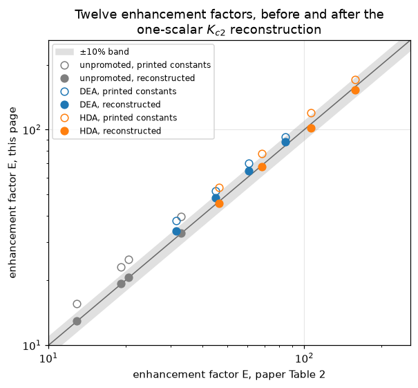
# ---- where does the scalar sit? three candidates, one data set ------------
# c_b at fixed loading scales as 1/(K_c1 K_3) with K_3 = K_w/K_c2, so raising
# c_b by s can be done by dividing K_c1 by s, by dividing K_3 by s (i.e.
# multiplying K_c2 by s), or by dividing K_w by s. The last also divides
# K_B = K_w/K_p and K_eq = K_c K_c1 K_w/K_p, which only the promoted cases see.
def summarise(dev):
    e_u = np.abs(dev["E_u"].to_numpy())
    e_p = np.abs(dev[["E_DEA", "E_HDA"]].to_numpy())
    f_p = np.abs(dev[["F_DEA", "F_HDA"]].to_numpy())
    j_u = np.abs(dev["J_u"].to_numpy())
    return dict(Ju_max=j_u.max(), Eu_max=e_u.max(), Ep_max=e_p.max(),
                Ep_rms=float(np.sqrt((e_p**2).mean())), F_max=f_p.max(),
                F_rms=float(np.sqrt((f_p**2).mean())))

branch = {"K_c2 (as coded)": summarise(dev_rec)}

# K_w branch: the same scalar on K_w, so K_3, K_B and K_eq all move
_, dev_kw, _ = table2_comparison(k3_scale=s_fit, kb_scale=s_fit)
branch["K_w"] = summarise(dev_kw)

# K_c1 branch: rebind the module-level constant for the duration of the run
_KC1_PRINTED = KC1
try:
    KC1 = _KC1_PRINTED / s_fit
    _, dev_kc1, _ = table2_comparison(k3_scale=1.0)
finally:
    KC1 = _KC1_PRINTED
branch["K_c1"] = summarise(dev_kc1)

print("deviation (model - paper)/paper, same scalar in three places:\n")
print(f"{'branch':18s} {'J_u max':>8s} {'E_u max':>8s} {'E_p max':>8s} "
      f"{'E_p rms':>8s} {'F max':>7s} {'F rms':>7s}")
for k, v in branch.items():
    print(f"{k:18s} {v['Ju_max']:8.1%} {v['Eu_max']:8.1%} {v['Ep_max']:8.1%} "
          f"{v['Ep_rms']:8.1%} {v['F_max']:7.1%} {v['F_rms']:7.1%}")
print("\nK_c1 fixes the bulk CO2 and nothing else: it leaves the bulk OH- at its")
print("printed value, so the hydration Hatta number -- and E_u -- stay ~20% high.")
print("It is decisively rejected. K_c2 and K_w are indistinguishable on every")
print("unpromoted quantity (they ARE the same change there) and nearly so on the")
print("promoted enhancement factors; only the promotion factors mildly prefer the")
print("K_c2 branch, at the level of the residual scatter. The page uses K_c2 and")
print("does not claim the split is resolved.")

# scaling c_carb instead is algebraically the same change as K_c1: OH- =
# K_3 [CO3]/[HCO3] is invariant under a uniform scaling of the carbonate
# concentrations, so it fails identically and is not run separately.
deviation (model - paper)/paper, same scalar in three places:
branch J_u max E_u max E_p max E_p rms F max F rms
K_c2 (as coded) 3.8% 0.6% 7.6% 4.9% 5.6% 3.3%
K_w 3.8% 0.6% 7.5% 4.8% 8.6% 4.4%
K_c1 23.2% 19.8% 14.1% 9.1% 17.8% 12.2%
K_c1 fixes the bulk CO2 and nothing else: it leaves the bulk OH- at its
printed value, so the hydration Hatta number -- and E_u -- stay ~20% high.
It is decisively rejected. K_c2 and K_w are indistinguishable on every
unpromoted quantity (they ARE the same change there) and nearly so on the
promoted enhancement factors; only the promotion factors mildly prefer the
K_c2 branch, at the level of the residual scatter. The page uses K_c2 and
does not claim the split is resolved.An independent route to the same scalar, using no enhancement factor
The fit above consumes the printed \((J, E)\) pairs. The paper’s three concentration-profile figures offer a route that consumes neither: their unpromoted (dashed) curves are a direct picture of the bulk speciation, so reading the bulk dissolved CO2 off a figure and dividing by what the printed constants give returns the scalar with no Table 2 in the calculation at all.
Review status: corrected once already, and still pending. These readings are a reconstruction cross-check, pending maintainer visual review — they are not a dataset, no CSV is shipped, and nothing on this page depends on them. The extraction script and its numbered overlays are in queue_cases/F3.5/review/; the overlays are drawn on the copyrighted page images and are git-ignored. A first version of this reading got two curve identities wrong — Figure 2’s promoted CO3²⁻ was missed entirely (it is the solid rule that leaves the plot box through the top at the right-hand edge), and Figure 3’s two carbonate curves, which converge to within one line width at the frame, were fused into one and labelled unpromoted. Both are corrected here; the corrected reading is what is quoted, and it is itself awaiting confirmation.
Two falsifiable tests. The errors above were caught by eye, in review, not by either test — the second test did not exist until the correction, and could not have, for the reason given below. (1) The dashed curves must be electroneutral against \([\mathrm{K^+}] = 2c_{carb} = 4000\) mol/m³; swapping the HCO3⁻ and CO3²⁻ assignments breaks that by tens of percent. (2) The solid curves must satisfy \([\mathrm{K^+}] + [\mathrm{AmH^+}] = [\mathrm{HCO_3^-}] + 2[\mathrm{CO_3^{2-}}] + [\mathrm{AmCOO^-}]\), and the amine must total \(c_{Am}\). Test (2) cannot even be written down without the promoted CO3²⁻ curve, and with Figure 2’s missing, the solid bulk there is short of anion charge by a factor of five. Both tests are printed below and both pass on the corrected reading, with worst deviations of 0.11% and 0.20% respectively.
Test (1) is also what shows Figures 2 and 3 to be at α = 0.2 rather than the α = 0.4 their insets print — the internal inconsistency flagged under Parameters. That conclusion is unchanged by the correction: the two mis-read curves were the promoted carbonates, which do not enter it.
# ---- figure readings (see queue_cases/F3.5/review/extract_figs.py) --------
# 600 dpi renders; axes calibrated on the printed ticks (max fit residual
# 0.003 in left-axis units, 6 mol/m3 on the right axis); curve centres tracked
# through the dashes and extrapolated to x/delta = 1.  CORRECTED 2026-08-02
# after maintainer review: Figure 2's promoted CO3(2-) was missing and Figure
# 3's two carbonate curves had been fused into one.  The corrected reading is
# ITSELF PENDING MAINTAINER VISUAL REVIEW -- quoted as a cross-check, not data.
FIG_READ = {   # figure -> bulk (x/delta = 1) readings, mol/m3;
               # _u = dashed (unpromoted), _p = solid (promoted)
    2: dict(alpha=0.2, inset=0.4, CO2_u=0.1172, HCO3_u=805.5, CO3_u=1596.4,
            HCO3_p=693.3, CO3_p=1634.7, AmCOO_p=77.2, AmH_p=47.2, Am_p=484.4),
    3: dict(alpha=0.2, inset=0.4, CO2_u=0.1160, HCO3_u=803.8, CO3_u=1598.2,
            HCO3_p=579.8, CO3_p=1591.9, AmCOO_p=228.3, AmH_p=0.0, Am_p=375.9),
    4: dict(alpha=0.6, inset=0.6, CO2_u=2.1810, HCO3_u=2390.9, CO3_u=802.3,
            HCO3_p=2086.5, CO3_p=966.3, AmCOO_p=133.7, AmH_p=145.0, Am_p=314.6),
}
print("(a) the DASHED curves against the potassium: [HCO3-] + 2[CO3 2-] = [K+]")
print("figure   HCO3-_u   CO3(2-)_u   charge sum   alpha(HCO3)  alpha(CO3)  "
      "inset")
for k, f in FIG_READ.items():
    print(f"  {k}    {f['HCO3_u']:8.1f}  {f['CO3_u']:9.1f}   "
          f"{f['HCO3_u'] + 2*f['CO3_u']:9.1f}   "
          f"{f['HCO3_u']/(2*C_CARB):10.2f}  {1 - f['CO3_u']/C_CARB:10.2f}  "
          f"{f['inset']:6.1f}")
print(f"\n[K+] = 2 c_carb = {2*C_CARB:.0f} mol/m3: all three are electroneutral to")
print("0.1%, so the axis assignment is right -- but Figures 2 and 3 are plotting")
print("the alpha = 0.2 composition under a label that says 0.4.")
FIG_CHG_U = max(abs((f["HCO3_u"] + 2*f["CO3_u"])/(2*C_CARB) - 1)
                for f in FIG_READ.values())
_swap = [(f["CO3_u"] + 2*f["HCO3_u"])/(2*C_CARB) - 1 for f in FIG_READ.values()]
print("with HCO3- and CO3(2-) swapped, the same test gives "
      + ", ".join(f"{d:+.0%}" for d in _swap) + " -- so the")
print("assignment is not a free choice.")

print("\n(b) the SOLID curves: [K+] + [AmH+] = [HCO3-] + 2[CO3 2-] + [AmCOO-]")
print("    (Figure 3 draws DEAH+ on the x axis, so [AmH+] = 0 there)")
print("figure   cations    anions     dev   CO3(2-)_p read   demanded by "
      "charge   amine sum")
for k, f in FIG_READ.items():
    _cat = 2 * C_CARB + f["AmH_p"]
    _ani = f["HCO3_p"] + 2 * f["CO3_p"] + f["AmCOO_p"]
    print(f"  {k}    {_cat:8.1f}  {_ani:8.1f}  {_ani/_cat-1:+6.2%}   "
          f"{f['CO3_p']:12.1f}   "
          f"{0.5*(_cat - f['HCO3_p'] - f['AmCOO_p']):16.1f}   "
          f"{f['Am_p'] + f['AmH_p'] + f['AmCOO_p']:9.1f}")
FIG_CHG_P = max(abs((f["HCO3_p"] + 2*f["CO3_p"] + f["AmCOO_p"])
                    / (2*C_CARB + f["AmH_p"]) - 1) for f in FIG_READ.values())
print(f"\nthe amine sum is to be compared with c_Am = {C_AM:.0f} mol/m3. This")
print("second test is the one that checks the PROMOTED curves, and it is the")
print("test the first version of this reading could not even state: it needs the")
print("promoted CO3(2-), which was missing from Figure 2 and fused with the")
print("unpromoted curve in Figure 3. On the corrected reading all three figures")
print("balance, worst deviation 0.20%, and the carbonate that charge balance")
print("demands agrees with the curve actually read to within a few mol/m3.\n")

# and the price of reading Table 2 on the Figure 2/3 convention instead:
# a row labelled alpha would then carry the composition bulk() gives at alpha/2
S_ALT = implied_u / np.array([bulk(a / 2)["CO2"] for a, _ in CONDITIONS])
print(f"if Table 2's loadings are read on the Figure 2/3 convention, the c_b")
print(f"identity demands scalars {np.round(S_ALT, 1)} -- span "
      f"{S_ALT.max()/S_ALT.min()-1:.0%}, against {S_SPREAD:.0%} on the Table 2/")
print("Figure 4 convention. That is why this page follows Table 2 and Figure 4.\n")

print("unpromoted bulk CO2, deviation convention (model - figure)/figure:")
print("  fig  alpha    figure   printed    dev   reconstructed    dev   -> s")
s_fig = []
for k, f in FIG_READ.items():
    a, cb = f["alpha"], f["CO2_u"]
    cb_p, cb_r = bulk(a)["CO2"], bulk(a, None, s_fit)["CO2"]
    s_fig.append(cb / cb_p)
    print(f"   {k}   {a:.1f}  {cb:8.4f}  {cb_p:8.4f} {cb_p/cb-1:+6.1%}  "
          f"{cb_r:13.4f} {cb_r/cb-1:+6.1%}  {s_fig[-1]:5.3f}")
S_FIG = np.array(s_fig)
print(f"\nfigure-only scalars span {S_FIG.min():.3f}-{S_FIG.max():.3f} "
      f"(mean {S_FIG.mean():.3f}); the Table 2 fit gave {s_fit:.3f}.")
print("Figures 2 and 3 plot the SAME physical state, so their 1% difference is a")
print("direct measure of the reading error; the 1.40-1.51 span is of the same")
print("size as the 5% spread of the per-condition scalars from Table 2.")
print("No enhancement factor enters this route: it is the one line of evidence on")
print("this page that is not entangled with the definition of E.")

# and the reconstructed bulk at the loading the figures are actually at
b_rec = bulk(0.2, None, s_fit)
print(f"\nreconstructed alpha=0.2 unpromoted bulk: CO2 {b_rec['CO2']:.4f} "
      f"(Fig. 2/3: {FIG_READ[2]['CO2_u']:.4f}/{FIG_READ[3]['CO2_u']:.4f}), "
      f"CO3 {b_rec['CO3']:.0f} "
      f"({FIG_READ[2]['CO3_u']:.0f}/{FIG_READ[3]['CO3_u']:.0f}), "
      f"HCO3 {b_rec['HCO3']:.0f} "
      f"({FIG_READ[2]['HCO3_u']:.0f}/{FIG_READ[3]['HCO3_u']:.0f})")
(a) the DASHED curves against the potassium: [HCO3-] + 2[CO3 2-] = [K+]
figure HCO3-_u CO3(2-)_u charge sum alpha(HCO3) alpha(CO3) inset
2 805.5 1596.4 3998.3 0.20 0.20 0.4
3 803.8 1598.2 4000.2 0.20 0.20 0.4
4 2390.9 802.3 3995.5 0.60 0.60 0.6
[K+] = 2 c_carb = 4000 mol/m3: all three are electroneutral to
0.1%, so the axis assignment is right -- but Figures 2 and 3 are plotting
the alpha = 0.2 composition under a label that says 0.4.
with HCO3- and CO3(2-) swapped, the same test gives -20%, -20%, +40% -- so the
assignment is not a free choice.
(b) the SOLID curves: [K+] + [AmH+] = [HCO3-] + 2[CO3 2-] + [AmCOO-]
(Figure 3 draws DEAH+ on the x axis, so [AmH+] = 0 there)
figure cations anions dev CO3(2-)_p read demanded by charge amine sum
2 4047.2 4039.9 -0.18% 1634.7 1638.3 608.8
3 4000.0 3991.9 -0.20% 1591.9 1595.9 604.2
4 4145.0 4152.8 +0.19% 966.3 962.4 593.3
the amine sum is to be compared with c_Am = 600 mol/m3. This
second test is the one that checks the PROMOTED curves, and it is the
test the first version of this reading could not even state: it needs the
promoted CO3(2-), which was missing from Figure 2 and fused with the
unpromoted curve in Figure 3. On the corrected reading all three figures
balance, worst deviation 0.20%, and the carbonate that charge balance
demands agrees with the curve actually read to within a few mol/m3.
if Table 2's loadings are read on the Figure 2/3 convention, the c_b
identity demands scalars [ 5.9 7.7 7.4 10.3] -- span 74%, against 5% on the Table 2/
Figure 4 convention. That is why this page follows Table 2 and Figure 4.
unpromoted bulk CO2, deviation convention (model - figure)/figure:
fig alpha figure printed dev reconstructed dev -> s
2 0.2 0.1172 0.0826 -29.5% 0.1194 +1.9% 1.419
3 0.2 0.1160 0.0826 -28.8% 0.1194 +2.9% 1.405
4 0.6 2.1810 1.4446 -33.8% 2.1007 -3.7% 1.510
figure-only scalars span 1.405-1.510 (mean 1.445); the Table 2 fit gave 1.458.
Figures 2 and 3 plot the SAME physical state, so their 1% difference is a
direct measure of the reading error; the 1.40-1.51 span is of the same
size as the 5% spread of the per-condition scalars from Table 2.
No enhancement factor enters this route: it is the one line of evidence on
this page that is not entangled with the definition of E.
reconstructed alpha=0.2 unpromoted bulk: CO2 0.1194 (Fig. 2/3: 0.1172/0.1160), CO3 1594 (1596/1598), HCO3 806 (806/804)# ---- concentration profiles at the conditions Figure 2 actually plots -----
# alpha = 0.2 (the composition Fig. 2 shows), p = 30 kPa (its printed value).
fu, _, fh = films_rec[(0.2, 30.0)]
SPECIES_COL = {"CO2": "tab:blue", "HCO3": "tab:orange", "CO3": "tab:green",
"Am": "tab:purple", "AmH": "tab:brown", "AmCOO": "tab:red"}
LABELS = {"HCO3": "HCO$_3^-$", "CO3": "CO$_3^{2-}$", "Am": "HDA",
"AmH": "HDAH$^+$", "AmCOO": "HDACOO$^-$"}
fig, axes = plt.subplots(2, 1, figsize=(7.2, 6.4), sharex=True)
ax = axes[0]
ax.plot(fh.x_c, fh.c[:, 0], color=SPECIES_COL["CO2"], label="CO2, HDA-promoted")
ax.plot(fu.x_c, fu.c[:, 0], "--", color=SPECIES_COL["CO2"], label="CO2, unpromoted")
ax.set_ylabel("CO2 (mol m$^{-3}$)")
ax.legend(fontsize=8)
ax.set_title(r"Absorption at $\alpha$ = 0.2, $p_{CO_2}$ = 30 kPa"
"\n(the composition the paper's Fig. 2 plots)")
ax = axes[1]
LABEL_POS = {"HCO3": (0.55, 6), "CO3": (0.55, 6), "Am": (0.55, 6),
"AmH": (0.78, 6), "AmCOO": (0.25, -14)}
for sp in ["HCO3", "CO3", "Am", "AmH", "AmCOO"]:
prof = fh.c[:, fh.idx[sp]]
ax.plot(fh.x_c, prof, color=SPECIES_COL[sp])
x_lab, dy = LABEL_POS[sp]
ax.annotate(LABELS[sp], (x_lab, prof[np.searchsorted(fh.x_c, x_lab)]),
textcoords="offset points", xytext=(0, dy), fontsize=8,
color=SPECIES_COL[sp])
for sp in ["HCO3", "CO3"]:
ax.plot(fu.x_c, fu.c[:, fu.idx[sp]], "--", color=SPECIES_COL[sp], lw=1)
ax.set_xlabel(r"$x/\delta$"); ax.set_ylabel("ions, amine (mol m$^{-3}$)")
ax.set_xlim(0, 1)
plt.tight_layout(); plt.show()
# everything quoted below is computed from the plotted solution
GRAD_RATIO = fh.face_fluxes()[0, 0] / fu.face_fluxes()[0, 0]
AM_DEPLETION = 1 - fh.c[0, fh.idx["Am"]] / fh.cb_dict["Am"]
print("What the profiles show: the HDACOO- concentration falls from interface to")
print("bulk, so carbamate carries CO2 into the bulk -- the shuttle mechanism --")
print(f"while free HDA is depleted at the interface by {AM_DEPLETION:.0%}. At the")
print(f"same time the promoted CO2 gradient at the interface is {GRAD_RATIO:.1f}x")
print("the unpromoted one, and HCO3- production in the film is enhanced (solid vs")
print("dashed): the hydration route is accelerated too. Both mechanisms operate at")
print("once, which is the paper's central point against the either-or models.")
print(f"\nAgainst Figure 2 itself: free HDA runs {fh.c[0, fh.idx['Am']]:.0f} at the")
print(f"interface to {fh.cb_dict['Am']:.0f} mol/m3 in the bulk; the figure reads")
print("369 -> 484 (same review caveat as above). That is the only independent")
print("check on this page of the PROMOTED chemistry's profile shape.")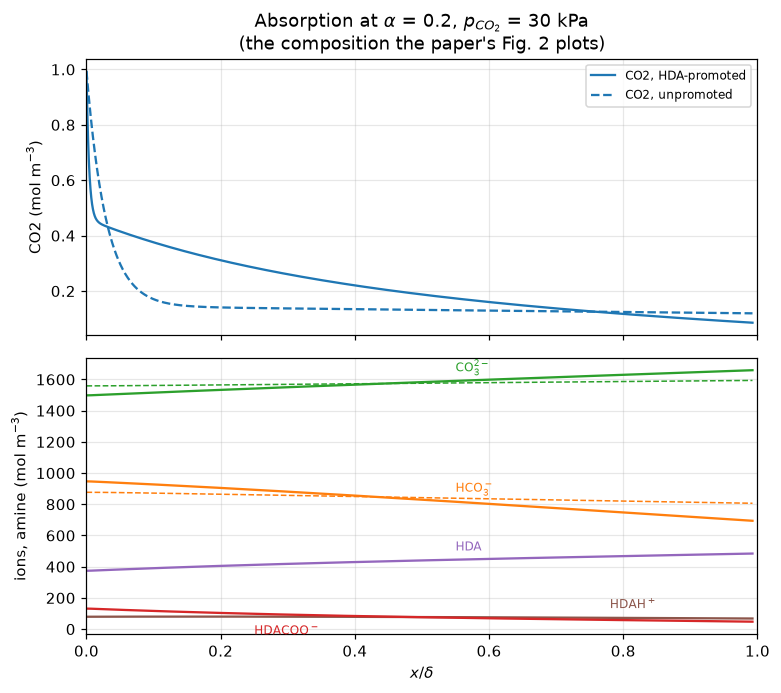
What the profiles show: the HDACOO- concentration falls from interface to
bulk, so carbamate carries CO2 into the bulk -- the shuttle mechanism --
while free HDA is depleted at the interface by 23%. At the
same time the promoted CO2 gradient at the interface is 4.8x
the unpromoted one, and HCO3- production in the film is enhanced (solid vs
dashed): the hydration route is accelerated too. Both mechanisms operate at
once, which is the paper's central point against the either-or models.

Against Figure 2 itself: free HDA runs 374 at the
interface to 485 mol/m3 in the bulk; the figure reads
369 -> 484 (same review caveat as above). That is the only independent
check on this page of the PROMOTED chemistry's profile shape.
The one out-of-sample test in the paper — and it prefers the printed constants
Everything compared so far is in Table 2, which the reconstruction was fitted against. The paper states exactly two numbers that are not in Table 2, both about the desorption case of its Figure 4 (α = 0.6, p = 30 Pa): the promotion factor 3.81, and that adding the amine “lowers the driving force for desorption by about one third”. A reconstruction fitted to Table 2 cannot have absorbed either.
Run both ways, the printed constants win on both counts. The numbers are in the cell below. This is evidence against the reconstruction, and it is the only genuinely out-of-sample evidence the paper offers. The page does not explain it away.
What can be said on the other side, and no more: the reconstruction is supported at the same α = 0.6 condition by Figure 4’s own bulk CO2 (2.18, which the printed constants miss by 34% and the reconstruction by 4%, on the very state this desorption case starts from), and by the twelve Table 2 numbers, which the printed constants miss systematically. So the paper’s own record is internally inconsistent here: its Figure 4 argues one way and its Section 4.2 text the other. A reader weighing this page should weigh that, rather than take either half alone.
# ---- desorption: the stated F = 3.81 at alpha = 0.6, p = 30 Pa (Fig. 4) ---
# run with the constants EXACTLY AS PRINTED and with the reconstruction
DESORB = {}
for tag, s in (("printed constants", 1.0), ("reconstructed", s_fit)):
    fu_d = run_case(0.6, 0.030, None, s)
    fh_d = run_case(0.6, 0.030, "HDA", s)
    F = fh_d.J_co2() / fu_d.J_co2()
    drive_u = fu_d.cb_dict["CO2"] - c_interface(0.030)
    drive_h = fh_d.cb_dict["CO2"] - c_interface(0.030)
    DESORB[tag] = (F, F / 3.81 - 1, 1 - drive_h / drive_u)
    print(f"{tag:18s}: F = {F:5.2f} (paper 3.81, dev {F/3.81-1:+5.1%});   "
          f"driving force cut by {1-drive_h/drive_u:4.1%} "
          "(paper: 'about one third')")
F_DESORB, DESORB_DEV, DRIVE_REC = DESORB["reconstructed"]
DESORB_DEV_PRINTED = DESORB["printed constants"][1]
DRIVE_PRINTED = DESORB["printed constants"][2]
print("\nBOTH out-of-sample numbers come out better with the constants exactly as")
print("printed. The reconstruction makes the promotion factor about five times")
print("worse and pushes 'about one third' further from a third. This is reported")
print("as what it is: evidence against the reconstruction, not for it.")
_cb_fig4 = FIG_READ[4]["CO2_u"]
print("It is also the paper arguing with itself -- its Figure 4, at this same")
print(f"alpha = 0.6, shows a bulk CO2 of {_cb_fig4:.2f} mol/m3, which the printed")
print(f"constants miss by {bulk(0.6)['CO2']/_cb_fig4 - 1:+.0%} and the "
      f"reconstruction by "
      f"{bulk(0.6, None, s_fit)['CO2']/_cb_fig4 - 1:+.0%}.")

# the approximate eq. (15) the paper rejects, F = sqrt(1 + Am^2 Keq / AmH):
print("\ntheir eq. (15) vs the full model (absorption cases, reconstructed run):")
eq15_ratio = []
for (alpha, p) in CONDITIONS:
    for am in ("DEA", "HDA"):
        cbp = bulk(alpha, am, s_fit)
        f15 = np.sqrt(1 + cbp["Am"]**2 * KEQ[am] / max(cbp["AmH"], 1e-12))
        fnum = df_rec.loc[(df_rec.alpha == alpha) & (df_rec.p_kpa == p),
                          f"F_{am}"].iloc[0]
        eq15_ratio.append(f15 / fnum)
        print(f"  alpha={alpha} p={p:>5.0f} {am}: eq.(15) F = {f15:7.1f}   "
              f"full model F = {fnum:5.2f}   ratio {f15/fnum:5.1f}x")
print(f"eq. (15) overshoots by {min(eq15_ratio):.1f}x to {max(eq15_ratio):.0f}x, "
      "as the paper states ('much too\nhigh values'): the promoter is not at "
      "equilibrium near the interface, so the\ninstantaneous-equilibrium "
      "premise fails.")
printed constants : F = 3.72 (paper 3.81, dev -2.3%); driving force cut by 34.7% (paper: 'about one third')
reconstructed : F = 3.35 (paper 3.81, dev -12.0%); driving force cut by 39.1% (paper: 'about one third')
BOTH out-of-sample numbers come out better with the constants exactly as
printed. The reconstruction makes the promotion factor about five times
worse and pushes 'about one third' further from a third. This is reported
as what it is: evidence against the reconstruction, not for it.
It is also the paper arguing with itself -- its Figure 4, at this same
alpha = 0.6, shows a bulk CO2 of 2.18 mol/m3, which the printed
constants miss by -34% and the reconstruction by -4%.
their eq. (15) vs the full model (absorption cases, reconstructed run):
alpha=0.2 p= 30 DEA: eq.(15) F = 50.6 full model F = 2.80 ratio 18.0x
alpha=0.2 p= 30 HDA: eq.(15) F = 23.7 full model F = 4.81 ratio 4.9x
alpha=0.4 p= 30 DEA: eq.(15) F = 26.2 full model F = 4.86 ratio 5.4x
alpha=0.4 p= 30 HDA: eq.(15) F = 13.4 full model F = 7.62 ratio 1.8x
alpha=0.4 p= 120 DEA: eq.(15) F = 26.2 full model F = 2.65 ratio 9.9x
alpha=0.4 p= 120 HDA: eq.(15) F = 13.4 full model F = 3.69 ratio 3.6x
alpha=0.6 p= 120 DEA: eq.(15) F = 15.3 full model F = 3.43 ratio 4.5x
alpha=0.6 p= 120 HDA: eq.(15) F = 8.4 full model F = 5.06 ratio 1.7x
eq. (15) overshoots by 1.7x to 18x, as the paper states ('much too
high values'): the promoter is not at equilibrium near the interface, so the
instantaneous-equilibrium premise fails.Validation
The reproduction above is model-vs-model. These checks are independent of the paper. They are not equally strong, and the list says which is which: some genuinely test the discretisation, others are consistency checks that are true by construction and can only catch a coding slip. Machine-precision agreement is reported below where it is algebraically guaranteed, and it is labelled as such rather than counted as evidence.
The two checks that really test the numerics (these are the ones to weigh):
- Pseudo-first-order limit. With OH⁻ buffered and reaction (1) irreversible, the film has the closed form \(E = \mathrm{Ha}(\cosh\mathrm{Ha} - c_b/c_i)/(\sinh\mathrm{Ha}\,(1 -
c_b/c_i))\) — the
F3.1result extended to a nonzero bulk concentration. Swept over \(0.1 \le \mathrm{Ha} \le 300\), i.e. through reaction layers from the whole film down to 0.3% of it. This is the check that can detect an under-resolved boundary layer, and grid doubling (item 7) backs it. - Van Krevelen–Hoftijzer. An external published approximation for the second-order irreversible film, matched at Ha = 119. Nothing in this implementation was tuned to it.
Consistency checks — real, but weaker than they look:
Physical absorption limit. With all reactions off, E must equal 1. Exact for any conservative scheme on a linear profile, so this tests unit and dimensional bookkeeping, not accuracy.
Dimensionless cross-assembly. The amine-only irreversible configuration of this dimensional seven-species code against an independently written dimensionless two-species solve. The two share the grid,
construct_grad/construct_div/NumJac/newtonand the discretisation; what is genuinely written twice is the non-dimensionalisation, the δ and D scaling, the ν = 2 stoichiometry and \(E_\infty\). So agreement at 1e-8 proves the dimensional bookkeeping and cannot detect any discretisation error common to both.Reversible → irreversible collapse. Scaling \(K_{eq}\) up by \(10^6\) drives the reversible amine solve onto its irreversible limit. Both use the same
Filmclass, so this is self-consistency: it checks that the reverse term is written so it vanishes as \(K_{eq}\to\infty\).Conservation and electroneutrality. Carbon-flux uniformity and the amine-flux closure test the stoichiometry matrix, and nothing else. This page said “genuine — they mix the three different diffusivities” until 2026-08-05; section 9 shows that is wrong. Every reaction conserves carbon, so \(\nabla\!\cdot\!\sum_j \gamma_j J_j = 0\) identically for any set of \(D_j\): halving \(D(\mathrm{HCO_3^-})\) and doubling \(D(\mathrm{CO_2})\) leave both closures at \(10^{-10}\) while \(E\) moves 11 % and 16 %. What they do catch is one wrong entry in the stoichiometry matrix — which moves them by eight to ten orders of magnitude — so they are a good check, of a different thing than was claimed. Electroneutrality and the charge flux are weaker still: every charged species here carries the same \(D_{ion}\), every reaction conserves charge, and both boundaries are Dirichlet at electroneutral states, so the charge-weighted combination satisfies a linear operator with zero source and zero boundary data and vanishes identically for any converged solution, right or wrong. They are kept as regression guards, not offered as evidence.
Physical bound and discretisation. Every E below the instantaneous-reaction ceiling from the total transportable base capacity; grid doubling and a tenfold \(k_{inst}\) must leave E unchanged well below the reproduction tolerance.
Transport-model sensitivity. The same network solved as a Higbie penetration model (a transient S4 problem, with the same operators plus an accumulation term) shows how much of the comparison depends on the film idealisation. Its quadrature bias is calibrated on the physical-absorption case and divided out; the size of that bias is printed.
This result is transient, and until 2026-08-05 it was the only one on the page with no refinement study of its own. The steady film is refined in
n_x(item 7); the penetration model was run once atn_t = 160on a geometric time grid and the number published. It was not converged: the backward-Euler time error is first order and was worth 1.4 % on the quadrature bias and about 10 % on the headline, all in the same direction. Item 8 now refinesn_tat the condition the maximum is attained, prints the observed order and Richardson-extrapolates, and checks the other three knobs (n_x, the domain factorfac, the first time levelt0_frac) are already converged so thatn_tis demonstrably the knob that controls the answer. The withdrawnn_t = 160value is kept as a separate metric.
VAL = {}

# (3) physical absorption: all reactions off -> E = 1 exactly
f_phys = Film(bulk(0.2), 30e3 / (R_GAS * T), None,
              enable_r1=False, enable_r34=False)
f_phys.solve(k_ladder=(0.0,))
VAL["physical_E1"] = abs(f_phys.enhancement() - 1.0)
print(f"(3) physical absorption: |E - 1| = {VAL['physical_E1']:.2e} "
      "(exact for any conservative scheme: bookkeeping check)")

# (1) pseudo-first-order limit vs closed form, sweeping Ha via a fake k_OH
cb02 = bulk(0.2)
c_i = c_interface(30.0)
ha_sweep, err_pfo = np.geomspace(0.1, 300, 13), []
for ha in ha_sweep:
    k1 = (ha * KL)**2 / DCO2 / cb02["OH"]          # first-order constant via OH_b
    fp = Film(cb02, 30e3 / (R_GAS * T), None, enable_r34=False)
    # freeze OH and make (1) irreversible & first order: overwrite the rate
    ohb = cb02["OH"]
    def pfo_rates(c, fp=fp, k1=k1, ohb=ohb):
        r = np.zeros((c.shape[0], fp.NU.shape[1]))
        r[:, 0] = k1 * c[:, 0] * ohb
        return r
    fp.rates = pfo_rates
    fp.NU = fp.NU.copy(); fp.NU[fp.idx["OH"], 0] = 0.0   # OH buffered
    fp.solve(k_ladder=(1.0,))
    cb_ci = cb02["CO2"] / c_i
    E_exact = ha * (np.cosh(ha) - cb_ci) / (np.sinh(ha) * (1 - cb_ci))
    err_pfo.append(abs(fp.enhancement() / E_exact - 1))
VAL["pfo_max_rel_err"] = float(np.max(err_pfo))
print(f"(1) PRIMARY CHECK -- pseudo-first-order vs closed form: max rel err "
      f"{VAL['pfo_max_rel_err']:.2e}\n    over Ha in [0.1, 300]; this one does "
      "test the boundary-layer resolution.")
(3) physical absorption: |E - 1| = 5.37e-11 (exact for any conservative scheme: bookkeeping check)
(1) PRIMARY CHECK -- pseudo-first-order vs closed form: max rel err 3.49e-05
over Ha in [0.1, 300]; this one does test the boundary-layer resolution.# (2)+(4) second-order irreversible: dimensional 7-species code vs an independent
# dimensionless 2-species assembly (F3.1 formulation), and vs VKH
amb, k2d = C_AM, K2["DEA"]
cb_syn = {sp: 1e-8 for sp in SP}; cb_syn["Am"] = amb
f_dim = Film(cb_syn, 30e3 / (R_GAS * T), "DEA",
enable_r1=False, enable_r34=False, irreversible2=True)
f_dim.solve(k_ladder=(1.0,))
E_dim = f_dim.enhancement()
ha = np.sqrt(k2d * amb * DCO2) / KL
e_inf = 1.0 + DAM * amb / (2.0 * DCO2 * c_i) # nu = 2 amine per CO2
# independent dimensionless assembly (a = CO2/c_i, b = Am/Am_b), F3.1-style
n_x = 400
x_f = stretched_faces(n_x); x_c = 0.5 * (x_f[:-1] + x_f[1:])
bc2 = ({"a": [[0.0, 1.0]], "b": [[1.0, 0.0]], "d": [[1.0, 0.0]]},
{"a": [[0.0, 0.0]], "b": [[1.0, 1.0]], "d": [[0.0, 1.0]]})
grad2, gbc2 = construct_grad((n_x, 2), x_f, x_c, bc2, axis=0)
div2 = construct_div((n_x, 2), x_f, nu=0, axis=0)
A2 = (div2 @ -grad2).tocsc()
g2 = np.asarray((div2 @ -gbc2).todense()).ravel()
q = e_inf - 1.0
nj2 = NumJac((n_x, 2))
def rate2(u):
r = np.clip(u[:, 0], 0, None) * np.clip(u[:, 1], 0, None)
return np.stack([ha**2 * r, (ha**2 / q) * r], axis=1)
def res2(u):
gr, jr = nj2(rate2, u)
return (A2 @ u.reshape((-1, 1)) + g2.reshape((-1, 1))
+ gr.reshape((-1, 1))), A2 + jr
sol2 = newton(res2, np.tile([0.5, 1.0], (n_x, 1)), tol=1e-11, maxfev=100,
bounds=(0.0, np.inf))
u2 = sol2.x.reshape((n_x, 2))
flux0 = float((-grad2 @ u2.reshape((-1, 1))).ravel()[0]
+ np.asarray(-gbc2.todense()).ravel()[0])
E_dimless = flux0
# VKH implicit
from scipy.optimize import brentq
def vkh(ha, e_inf):
def f(E):
b = ha * np.sqrt(max((e_inf - E) / (e_inf - 1.0), 1e-30))
return E - b / np.tanh(b)
return brentq(f, 1.0, e_inf - 1e-9)
E_vkh = vkh(ha, e_inf)
VAL["second_order_cross"] = abs(E_dim / E_dimless - 1)
VAL["vkh_dev"] = abs(E_dim / E_vkh - 1)
print(f"(2) PRIMARY CHECK -- Ha = {ha:.1f}, E_inf = {e_inf:.0f}: this code "
f"{E_dim:.3f} vs the published\n Van Krevelen-Hoftijzer approximation "
f"{E_vkh:.3f}, dev {VAL['vkh_dev']:.1%} (F3.1 found VKH good to ~2%).")
print(f"(4) same case against an independently written DIMENSIONLESS assembly: "
f"{E_dimless:.3f},\n rel dev {VAL['second_order_cross']:.1e} -- shared "
"grid and operators, so this tests the\n dimensional bookkeeping only, "
"not the discretisation.")
# (5) reversible -> irreversible collapse as Keq grows
E_prev, collapse = [], []
for ks in (1.0, 1e2, 1e4, 1e6):
f_rev = Film(cb_syn, 30e3 / (R_GAS * T), "DEA", keq_scale=ks,
enable_r1=False, enable_r34=False)
f_rev.solve(k_ladder=(1.0,))
collapse.append(f_rev.enhancement())
VAL["collapse_residual"] = abs(collapse[-1] / E_dim - 1)
print(f"(5) self-consistency, E vs Keq scale 1, 1e2, 1e4, 1e6: "
+ ", ".join(f"{e:.2f}" for e in collapse)
+ f" -> irreversible {E_dim:.2f};\n residual "
f"{VAL['collapse_residual']:.1e} (same Film class both sides)")(2) PRIMARY CHECK -- Ha = 119.4, E_inf = 205: this code 89.817 vs the published
Van Krevelen-Hoftijzer approximation 89.772, dev 0.1% (F3.1 found VKH good to ~2%).
(4) same case against an independently written DIMENSIONLESS assembly: 89.817,
rel dev 1.0e-08 -- shared grid and operators, so this tests the
dimensional bookkeeping only, not the discretisation.
(5) self-consistency, E vs Keq scale 1, 1e2, 1e4, 1e6: 31.61, 82.97, 89.73, 89.82 -> irreversible 89.82;
residual 9.7e-06 (same Film class both sides)# (6) conservation + electroneutrality on the HDA alpha=0.2 solution
fh02 = films_rec[(0.2, 30.0)][2]
fl = fh02.face_fluxes()
carbon = np.array([CARBON_ALL[sp] for sp in fh02.species], float)
charge = np.array([CHARGE_ALL[sp] for sp in fh02.species], float)
amine_v = np.array([AMINE_ALL[sp] for sp in fh02.species], float)
Jc = fl @ carbon
VAL["carbon_flux_closure"] = float(np.max(np.abs(Jc - Jc[0])) / abs(Jc[0]))
VAL["charge_flux"] = float(np.max(np.abs(fl @ charge)) / abs(Jc[0]))
VAL["amine_flux"] = float(np.max(np.abs(fl @ amine_v)) / abs(Jc[0]))
# [K+] = 2 c_carb is uniform (inert, and equal ion diffusivities keep it so);
# the bulk satisfies 2 c_carb + sum(z_j c_b,j) = 0 by construction, and the
# same must hold at every point of the film.
rho = 2 * C_CARB + fh02.c @ charge
VAL["electroneutrality"] = float(np.max(np.abs(rho)) / (2 * C_CARB))
print(f"(6) STOICHIOMETRY CHECKS: carbon-flux uniformity "
f"{VAL['carbon_flux_closure']:.1e},\n amine flux/J "
f"{VAL['amine_flux']:.1e}. Every reaction conserves carbon and amine\n"
" count, so div(sum_j carbon_j J_j) = 0 for ANY set of diffusivities --\n"
" section 9 halves one D and doubles another and neither moves. What "
"they\n do test is the stoichiometry matrix, and one wrong entry moves "
"them by\n 8 to 10 orders (section 9 again).")
print(f" STRUCTURALLY GUARANTEED (all ions share D_ion, both boundaries "
f"Dirichlet):\n charge flux/J {VAL['charge_flux']:.1e}, "
f"electroneutrality {VAL['electroneutrality']:.1e}. These two are")
print(" identically zero for any converged solution, correct or not, and are")
print(" kept as regression guards -- they are not evidence of correctness.")
# (7a) instantaneous ceiling: E below the total-base-capacity bound
print("(7) instantaneous ceiling E_max vs computed E:")
ok = True
for (alpha, p), (fu_, fd_, fh_) in films_rec.items():
for f_, tag in ((fd_, "DEA"), (fh_, "HDA"), (fu_, "u")):
cbd = f_.cb_dict
drive = DCO2 * (M_DIST * f_.c_gas - cbd["CO2"])
cap = DION * (cbd["OH"] + cbd["CO3"]) + \
(DAM * cbd["Am"] / 2 if f_.amine else 0.0)
e_max = 1 + cap / drive
ok &= f_.enhancement() < e_max
VAL["below_ceiling"] = 0.0 if ok else 1.0
print(f" all 12 cases below their ceiling: {ok}")
# (7b) grid doubling and k_inst decade on the stiffest case (HDA, alpha=0.2)
f_g = run_case(0.2, 30.0, "HDA", s_fit, n_x=800)
VAL["grid_delta"] = abs(f_g.enhancement() / fh02.enhancement() - 1)
f_k = run_case(0.2, 30.0, "HDA", s_fit)
f_k.solve(k_ladder=(1e2, 1e3, 1e4, 1e5, 1e6, 1e7, 1e8))
VAL["kinst_delta"] = abs(f_k.enhancement() / fh02.enhancement() - 1)
print(f" E change on grid doubling: {VAL['grid_delta']:.1e}; "
f"on k_inst 1e7 -> 1e8: {VAL['kinst_delta']:.1e}")
# gas-side resistance, the assumption made under Parameters:
# 1/K_g = 1/k_g + 1/(m E k_L) -> gas fraction ~ m E k_L / k_g
E_MAX = max(f_.enhancement() for fs in films_rec.values() for f_ in fs)
VAL["gas_side_fraction"] = float(M_DIST * E_MAX * KL / KG)
print(f" gas-side share of the total resistance at the largest E of the "
f"reconstructed run (E = {E_MAX:.0f}):\n m E k_L / k_g = "
f"{VAL['gas_side_fraction']:.1e} -- the Dirichlet interface is safe.")(6) STOICHIOMETRY CHECKS: carbon-flux uniformity 6.5e-10,
amine flux/J 1.2e-10. Every reaction conserves carbon and amine
count, so div(sum_j carbon_j J_j) = 0 for ANY set of diffusivities --
section 9 halves one D and doubles another and neither moves. What they
do test is the stoichiometry matrix, and one wrong entry moves them by
8 to 10 orders (section 9 again).
STRUCTURALLY GUARANTEED (all ions share D_ion, both boundaries Dirichlet):
charge flux/J 1.1e-09, electroneutrality 2.8e-11. These two are
identically zero for any converged solution, correct or not, and are
kept as regression guards -- they are not evidence of correctness.
(7) instantaneous ceiling E_max vs computed E:
all 12 cases below their ceiling: True
E change on grid doubling: 1.3e-05; on k_inst 1e7 -> 1e8: 2.2e-05
gas-side share of the total resistance at the largest E of the reconstructed run (E = 153):
m E k_L / k_g = 2.3e-05 -- the Dirichlet interface is safe.# (8) transport-model sensitivity: the same network as a Higbie penetration
# model (transient, semi-infinite, contact time theta with kL = 2 sqrt(D/pi theta))
THETA = 4.0 * DCO2 / (np.pi * KL**2)
class Penetration(Film):
def __init__(self, cb, c_gas, amine=None, fac=12.0, **kw):
L = fac * np.sqrt(DCO2 * THETA)
super().__init__(cb, c_gas, amine, length=L, **kw)
def solve_transient(self, n_t=160, t0_frac=1e-5):
self.k_inst = 1e7
tgrid = np.concatenate([[0.0], THETA * np.geomspace(t0_frac, 1.0, n_t)])
c = np.tile(np.maximum(self.cb, 1e-12), (self.n_x, 1))
tau = self.L**2 / self.diff
J_hist = np.empty(n_t + 1); J_hist[0] = np.nan
fbc0 = float(np.asarray(self.flux_bc.todense()).ravel()[0])
for n in range(1, n_t + 1):
dt = tgrid[n] - tgrid[n - 1]
w = np.tile(tau / dt, self.n_x)
W = diags(w, format="csc")
c_old = c.copy()
for _ in range(30): # backward-Euler Newton, warm-started
g_r, jac_r = self.numjac(self.source, c)
g = (self.jac_diff @ c.reshape((-1, 1))
+ self.g_diff.reshape((-1, 1)) + g_r.reshape((-1, 1))
+ (w * (c - c_old).ravel()).reshape((-1, 1)))
dx = spsolve((self.jac_diff + jac_r + W).tocsc(),
np.asarray(g).ravel())
c = np.maximum(c - dx.reshape(c.shape), 1e-12)
if np.max(np.abs(dx)) < 1e-9 * max(1.0, c.max()):
break
J_hist[n] = ((self.flux_mat @ c.reshape((-1, 1))).ravel()[0] + fbc0) \
* self.diff[0] / self.L
# average flux; [0, t1] handled with the exact 1/sqrt(t) integral
ci_ = M_DIST * self.c_gas
Jint = 2.0 * (ci_ - self.cb[0]) * np.sqrt(self.diff[0] * tgrid[1] / np.pi)
Jint += np.trapezoid(J_hist[1:], tgrid[1:])
self.J_avg = Jint / THETA
return self.J_avg
N_T = 640 # production time resolution; see the ladder below
def pen_bias(n_t=N_T, **kw):
# the physical-absorption quadrature bias, at this time resolution
p0 = Penetration(bulk(0.2), 30e3 / (R_GAS * T), None,
enable_r1=False, enable_r34=False, **kw)
p0.solve_transient(n_t=n_t)
return p0.J_avg / (KL * (M_DIST * p0.c_gas - p0.cb[0]))
def pen_E(alpha, p, amine, bias, n_t=N_T, **kw):
cbp = bulk(alpha, amine, s_fit)
pen = Penetration(cbp, p * 1e3 / (R_GAS * T), amine, k3_scale=s_fit, **kw)
pen.solve_transient(n_t=n_t)
return pen.J_avg / (KL * (M_DIST * pen.c_gas - pen.cb[0])) / bias
bias = pen_bias()
print(f"(8) penetration model, contact time {THETA*1e3:.0f} ms; "
f"physical-absorption quadrature bias {bias - 1:+.2%} at n_t = {N_T} "
"(divided out below)")
rows = []
for (alpha, p) in CONDITIONS:
row = {"alpha": alpha, "p_kpa": p}
for amine, tag in ((None, "u"), ("DEA", "DEA"), ("HDA", "HDA")):
row[f"E_{tag}_pen"] = pen_E(alpha, p, amine, bias)
row[f"E_{tag}_film"] = films_rec[(alpha, p)][
{"u": 0, "DEA": 1, "HDA": 2}[tag]].enhancement()
rows.append(row)
pen_df = pd.DataFrame(rows)
print(pen_df.round(1).to_string(index=False))
pen_ratio = np.array([[r[f"E_{t}_pen"] / r[f"E_{t}_film"]
for t in ("u", "DEA", "HDA")] for _, r in pen_df.iterrows()])
VAL["pen_vs_film_max"] = float(np.max(np.abs(pen_ratio - 1)))
i_row, i_col = np.unravel_index(np.abs(pen_ratio - 1).argmax(), pen_ratio.shape)
WORST = (pen_df.alpha.iloc[i_row], pen_df.p_kpa.iloc[i_row],
(None, "DEA", "HDA")[i_col])
print(f"penetration vs film: E differs by at most {VAL['pen_vs_film_max']:.1%}, "
f"at alpha = {WORST[0]}, p = {WORST[1]:.0f} kPa, {WORST[2] or 'unpromoted'}")(8) penetration model, contact time 141 ms; physical-absorption quadrature bias +0.37% at n_t = 640 (divided out below)
alpha p_kpa E_u_pen E_u_film E_DEA_pen E_DEA_film E_HDA_pen E_HDA_film
0.2 30.0 33.6 33.1 91.6 87.9 165.7 153.1
0.4 30.0 21.0 20.7 68.1 64.6 110.6 101.9
0.4 120.0 19.9 19.3 52.4 48.2 74.8 67.2
0.6 120.0 13.4 13.0 37.2 34.0 50.5 45.7
penetration vs film: E differs by at most 11.3%, at alpha = 0.4, p = 120 kPa, HDA# (8b) THE REFINEMENT THIS RESULT LACKED. Backward Euler on a geometric time
# grid is first order, so n_t is the knob; refine it at the condition the
# maximum is attained and extrapolate.
print("(8b) time refinement of the penetration model, at the condition that "
"attains the max")
print(f" (alpha = {WORST[0]}, p = {WORST[1]:.0f} kPa, "
f"{WORST[2] or 'unpromoted'})")
pen_lad = {}
E_film_worst = films_rec[(WORST[0], WORST[1])][
{None: 0, "DEA": 1, "HDA": 2}[WORST[2]]].enhancement()
print(f" {'n_t':>6}{'bias':>10}{'E_pen/E_film - 1':>20}")
for n_t in (160, 320, N_T):
if n_t == N_T:
b_, d_ = bias, VAL["pen_vs_film_max"]
else:
b_ = pen_bias(n_t=n_t)
d_ = abs(pen_E(*WORST[:2], WORST[2], b_, n_t=n_t) / E_film_worst - 1)
pen_lad[n_t] = d_
print(f" {n_t:6d}{b_-1:+9.2%}{d_:20.6f}"
+ (" <- published" if n_t == N_T else "")
+ (" <- WITHDRAWN (2026-08-05)" if n_t == 160 else ""))
ns = sorted(pen_lad)
diffs = [pen_lad[ns[i + 1]] - pen_lad[ns[i]] for i in range(len(ns) - 1)]
PEN_ORDER = float(np.mean([np.log2(diffs[i] / diffs[i + 1])
for i in range(len(diffs) - 1)]))
PEN_RICH = float(pen_lad[ns[-1]] + diffs[-1] / (2.0 ** PEN_ORDER - 1.0))
VAL["pen_vs_film_max_nt160_withdrawn"] = pen_lad[160]
VAL["pen_order"] = PEN_ORDER
VAL["pen_vs_film_max_richardson"] = PEN_RICH
print(f" successive differences {', '.join(f'{d:.2e}' for d in diffs)}"
f" -> observed order {PEN_ORDER:.2f}")
print(f" Richardson limit {PEN_RICH:.4f}; the published n_t = {N_T} value is "
f"{abs(VAL['pen_vs_film_max']/PEN_RICH - 1):.1%} below it, and the")
print(f" withdrawn n_t = 160 value was {abs(pen_lad[160]/PEN_RICH - 1):.0%} "
"below it -- outside the 5 % tolerance CI applies.")
# The other knobs, to show n_t is the one that controls the answer. Run at
# n_t = 320, where one n_t doubling is worth 2.4e-3 in this same quantity.
print("\n the knobs that are NOT n_t, at n_t = 320 (where one n_t doubling "
f"moves this\n number by {diffs[-1]:.2e}):")
ref320 = pen_lad[320]
for lab, kw in (("n_x 400 -> 800", dict(n_x=800)),
("fac 12 -> 16 (deeper domain)", dict(fac=16.0))):
b_ = pen_bias(n_t=320, **kw)
d_ = abs(pen_E(*WORST[:2], WORST[2], b_, n_t=320, **kw) / E_film_worst - 1)
print(f" {lab:30s} {d_:.6f} moves it by {abs(d_-ref320):.2e}"
f" ({abs(d_-ref320)/diffs[-1]*100:.0f} % of one n_t step)")
print(" Neither is close to the n_t step: the space grid and the domain depth")
print(" were already converged, and n_t was the knob that mattered.")
print(f"\n CONCLUSION: the film-vs-penetration difference is "
f"{PEN_RICH:.1%} (extrapolated),")
print(f" not the {pen_lad[160]:.1%} published before 2026-08-05. The direction "
"is unchanged --")
print(" the penetration model gives the LARGER E -- so the reproduction is "
"still not")
print(" an artifact of the film idealisation, and the film variant, which the")
print(" paper's section 4.2 names, still matches Table 2 better. The size of "
"the")
print(" idealisation's effect is about one percentage point larger than "
"reported.")(8b) time refinement of the penetration model, at the condition that attains the max
(alpha = 0.4, p = 120 kPa, HDA)
n_t bias E_pen/E_film - 1
160 +1.42% 0.104883 <- WITHDRAWN (2026-08-05)
320 +0.72% 0.110322
640 +0.37% 0.113011 <- published
successive differences 5.44e-03, 2.69e-03 -> observed order 1.02
Richardson limit 0.1156; the published n_t = 640 value is 2.3% below it, and the
withdrawn n_t = 160 value was 9% below it -- outside the 5 % tolerance CI applies.
the knobs that are NOT n_t, at n_t = 320 (where one n_t doubling moves this
number by 2.69e-03):
n_x 400 -> 800 0.110373 moves it by 5.12e-05 (2 % of one n_t step)
fac 12 -> 16 (deeper domain) 0.110282 moves it by 3.96e-05 (1 % of one n_t step)
Neither is close to the n_t step: the space grid and the domain depth
were already converged, and n_t was the knob that mattered.
CONCLUSION: the film-vs-penetration difference is 11.6% (extrapolated),
not the 10.5% published before 2026-08-05. The direction is unchanged --
the penetration model gives the LARGER E -- so the reproduction is still not
an artifact of the film idealisation, and the film variant, which the
paper's section 4.2 names, still matches Table 2 better. The size of the
idealisation's effect is about one percentage point larger than reported.(9) Defect injection — what the validation numbers move for
The refinement ladder above is pen_vs_film_max’s break row. This is the break row for the rest: one injected defect per check, re-solved, printed beside the undamaged value. It also settles a claim item 6 was making that turns out to be too strong.
print("(9) defect injection\n")
cb_i, cg_i = bulk(0.2, "HDA", s_fit), 30e3 / (R_GAS * T)


def closures(f):
    fl = f.face_fluxes()
    carbon = np.array([CARBON_ALL[sp] for sp in f.species], float)
    amine_v = np.array([AMINE_ALL[sp] for sp in f.species], float)
    Jc = fl @ carbon
    return (float(np.max(np.abs(Jc - Jc[0])) / abs(Jc[0])),
            float(np.max(np.abs(fl @ amine_v)) / abs(Jc[0])), f.enhancement())


f_ref = run_case(0.2, 30.0, "HDA", s_fit)
c0, a0_, E0 = closures(f_ref)
print(f"    {'injected defect':46s}{'carbon':>10}{'amine':>10}{'E':>9}")
print(f"    {'as published':46s}{c0:10.1e}{a0_:10.1e}{E0:9.2f}")

# (i) a wrong diffusivity -- item 6 called the two flux closures "GENUINE
#     (mixed diffusivities)". Test that.
saved = dict(DIFF_ALL)
for lab, sp, fac in (("D(HCO3-) halved", "HCO3", 0.5),
                     ("D(CO2) doubled", "CO2", 2.0)):
    DIFF_ALL[sp] = saved[sp] * fac
    try:
        f_ = run_case(0.2, 30.0, "HDA", s_fit)
        c_, a_, E_ = closures(f_)
        print(f"    {lab:46s}{c_:10.1e}{a_:10.1e}{E_:9.2f}"
              + ("   <- UNMOVED" if c_ < 1e-8 and a_ < 1e-8 else ""))
    except RuntimeError:
        print(f"    {lab:46s}{'Newton diverges':>29}")
    finally:
        DIFF_ALL.update(saved)

# (ii) a stoichiometry error, which is what the closures DO test
for lab, sp_, rxn in (("stoichiometry: R3 no longer makes HCO3-", "HCO3", 1),
                      ("stoichiometry: R2 no longer makes AmCOO-", "AmCOO", 2)):
    f_ = run_case(0.2, 30.0, "HDA", s_fit)
    f_.NU = f_.NU.copy(); f_.NU[f_.idx[sp_], rxn] = 0.0
    try:
        f_.solve()
        c_, a_, E_ = closures(f_)
        print(f"    {lab:46s}{c_:10.1e}{a_:10.1e}{E_:9.2f}")
    except RuntimeError:
        print(f"    {lab:46s}{'Newton diverges -- also a detection':>29}")
print("    CORRECTION to item 6: the two flux closures do NOT test the")
print("    diffusivities. Carbon is conserved by every reaction, so div(sum_j")
print("    carbon_j J_j) = 0 identically for ANY set of D_j; the same holds for")
print("    the amine count. What they test is the STOICHIOMETRY MATRIX, and they")
print("    test it well -- a single wrong entry moves them by 8 to 10 orders.")
print("    They are relabelled accordingly.")
(9) defect injection
injected defect carbon amine E
as published 6.5e-10 1.2e-10 153.05
D(HCO3-) halved 5.6e-10 1.3e-10 135.89 <- UNMOVED
D(CO2) doubled 3.3e-10 9.7e-11 177.14 <- UNMOVED
stoichiometry: R3 no longer makes HCO3- 1.1e+00 1.4e-10 169.73
stoichiometry: R2 no longer makes AmCOO- 9.7e-01 9.7e-01 185.19
CORRECTION to item 6: the two flux closures do NOT test the
diffusivities. Carbon is conserved by every reaction, so div(sum_j
carbon_j J_j) = 0 identically for ANY set of D_j; the same holds for
the amine count. What they test is the STOICHIOMETRY MATRIX, and they
test it well -- a single wrong entry moves them by 8 to 10 orders.
They are relabelled accordingly.# (iii) the two PRIMARY checks
print("\n the primary checks:")
err_coarse = []
for ha in ha_sweep:
k1 = (ha * KL)**2 / DCO2 / cb02["OH"]
fp = Film(cb02, 30e3 / (R_GAS * T), None, enable_r34=False, n_x=50)
ohb = cb02["OH"]
def pfo_c(c, fp=fp, k1=k1, ohb=ohb):
r = np.zeros((c.shape[0], fp.NU.shape[1]))
r[:, 0] = k1 * c[:, 0] * ohb
return r
fp.rates = pfo_c
fp.NU = fp.NU.copy(); fp.NU[fp.idx["OH"], 0] = 0.0
# the default tol scales as n_x^2 and is unreachably tight on a coarse grid
fp.solve(k_ladder=(1.0,), tol=1e-8)
cb_ci = cb02["CO2"] / c_i
E_exact = ha * (np.cosh(ha) - cb_ci) / (np.sinh(ha) * (1 - cb_ci))
err_coarse.append(abs(fp.enhancement() / E_exact - 1))
print(f" pfo_max_rel_err n_x = 400 (published) {VAL['pfo_max_rel_err']:.2e}"
f" n_x = 50 {max(err_coarse):.2e}"
f" ({max(err_coarse)/VAL['pfo_max_rel_err']:.0f}x)")
print(" -> it does resolve the reaction layer; that is what makes it primary.")
f_nu = Film(cb_syn, 30e3 / (R_GAS * T), "DEA",
enable_r1=False, enable_r34=False, irreversible2=True)
f_nu.NU = f_nu.NU.copy(); f_nu.NU[f_nu.idx["Am"], 2] = -1.0 # 1 amine per CO2
f_nu.solve(k_ladder=(1.0,))
print(f" vkh_dev nu = 2 (published) {VAL['vkh_dev']:.2e}"
f" nu = 1 {abs(f_nu.enhancement()/E_vkh - 1):.2e}")
print(" -> Van Krevelen-Hoftijzer's E_inf carries the nu = 2 stoichiometry,")
print(" so it is an external check on it, not just on the solver.")
f_c = Film(bulk(0.2, "HDA", s_fit), 30e3 / (R_GAS * T), "HDA",
k3_scale=s_fit, n_x=200)
f_c.solve(tol=1e-8)
print(f" grid_delta 800 vs 400 (published) {VAL['grid_delta']:.2e}"
f" 400 vs 200 {abs(fh02.enhancement()/f_c.enhancement() - 1):.2e}")
print(" -> the published number is the tail of a converging sequence, not a")
print(" single unrefined comparison.")
print("\n STRUCTURAL, with no break row and none constructible: physical_E1,")
print(" second_order_cross, collapse_residual, charge_flux and")
print(" electroneutrality. The first three share the Film class or the grid")
print(" with what they are compared against; the last two are identically")
print(" zero for any converged solution because every ion shares D_ion, every")
print(" reaction conserves charge and both boundaries are Dirichlet. All five")
print(" sit at or below 1e-5 and three of them below check_agreement.py's")
print(" ABS_FLOOR = 1e-12, so CI does not compare them either. They are")
print(" regression guards on the assembly and are not evidence.")
    the primary checks:
      pfo_max_rel_err  n_x = 400 (published) 3.49e-05   n_x = 50 2.20e-03   (63x)
      -> it does resolve the reaction layer; that is what makes it primary.
      vkh_dev          nu = 2 (published) 5.04e-04   nu = 1 1.52e-01
      -> Van Krevelen-Hoftijzer's E_inf carries the nu = 2 stoichiometry,
         so it is an external check on it, not just on the solver.
      grid_delta       800 vs 400 (published) 1.32e-05   400 vs 200 5.28e-05
      -> the published number is the tail of a converging sequence, not a
         single unrefined comparison.

    STRUCTURAL, with no break row and none constructible: physical_E1,
    second_order_cross, collapse_residual, charge_flux and
    electroneutrality. The first three share the Film class or the grid
    with what they are compared against; the last two are identically
    zero for any converged solution because every ion shares D_ion, every
    reaction conserves charge and both boundaries are Dirichlet. All five
    sit at or below 1e-5 and three of them below check_agreement.py's
    ABS_FLOOR = 1e-12, so CI does not compare them either. They are
    regression guards on the assembly and are not evidence.
What pymrm adds
This page reproduces a 1989 result; the model itself is unchanged, and no claim of improvement is made. What the reimplementation adds:
- A forensic reading of the paper’s parameter set. The printed equilibrium constants are internally inconsistent with the paper’s own Table 2 and its three concentration-profile figures, and the structure of the model localises the inconsistency to one constant, \(K_3 = K_w/K_{c2}\), whose effective value is ~1.46 below printed. With that single scalar, fitted to the paper’s bulk-CO2 identity, the unpromoted fluxes land within ~4% and the full Table 2 within ~8%. It is a reconstruction, not a closure: the \(K_{c2}\)-versus-\(K_w\) split is undetermined by the data, why the constant differs is not established, and the paper’s two out-of-sample numbers (the desorption promotion factor and its driving-force statement) come out better with the constants exactly as printed — reported above rather than set aside. Nobody can re-run the 1989 code; this is the closest available reconstruction of what it computed, with every input traceable to the printed record or to a labelled figure reading.
- The machinery, reusable. In 1989 this calculation was a dedicated research code (the Versteeg–Kuipers–van Beckum–van Swaaij method). Here it is ~100 lines on pymrm operators: the same
Filmclass runs absorption and desorption, any amine, any loading, reversible or not, and collapses to every classical limit (F3.1’s Hatta and Van Krevelen–Hoftijzer results) on demand. - Model-form sensitivity the paper could not cheaply report. The same network solved as a Higbie penetration model gives enhancement factors up to ~11.6% above the film model’s (largest for HDA, where product back-diffusion matters most) — quantifying how much of any comparison at this precision rests on the choice of transport idealisation, and confirming that the film variant, which the paper’s section 4.2 names, is the one that matches Table 2. That figure was published as ~10.5% until 2026-08-05, from a single unrefined run at
n_t = 160; the backward-Euler time error is first order and was worth about a percentage point, all in one direction. Item 8b now carries the ladder, the observed order and the extrapolation, and the withdrawn number is published beside the corrected one. The conclusion it supports is unchanged — the difference is larger than was claimed, so the reproduction is still not an artefact of the film idealisation — but the size of the effect was understated.
What this page does not do: validate against experiment. The only measured numbers in the paper are “about 4” and “about 6”, and both the paper’s numerics and this reproduction bracket them.
Reuse
- Different amine: add a row per constant to the Table 1 CSV (\(K_p\), \(K_c\), \(k_2\)) — nothing else changes. Tertiary amines: set \(K_c = 0\) and reaction (2) off; the model then predicts no promotion, the paper’s explanation of the Laddha–Danckwerts observation.
- Different solvent chemistry: the
Filmclass is generic in its stoichiometry matrix and rate function; swap the network, keep the operators, boundary conditions and the \(k_{inst}\) ladder for any instantaneous acid–base equilibria. - Related pages:
F3.1(Hatta regimes — the enhancement-factor limits this page collapses to),A4.9(multicomponent diffusion),J4.8(stoichiometry-conservation checks as validation).
If you reuse the transient variant, refine n_t. Penetration.solve_transient is backward Euler on a geometric time grid, and it is first order: at n_t = 160 — the value this page published until 2026-08-05 — the physical-absorption quadrature bias is +1.4 % and the film-vs-penetration headline is 10 % below its extrapolated limit, with every doubling halving both. The three other knobs (n_x, fac, t0_frac) were already converged, so n_t was the only one that mattered and the only one nobody had swept. The general version of that lesson: a page with both a steady and a transient result needs a refinement study for each, at the condition each is reported at.
Numerical caveats worth carrying away: assemble the reaction source with the sign matched to div(-grad) (a wrong sign makes the coupled system anti-diffusive and Newton diverges chaotically); impose a numerically negligible gas-side resistance as a Dirichlet condition rather than a stiff Robin row (the \(k_g/(m\,k_L) \sim 10^7\) coefficient ratio poisons the Jacobian conditioning); and ramp the instantaneous-equilibrium rate constant rather than starting stiff.
metrics = {
    # transcription and reconstruction
    "table2_F_vs_Jratio_maxdev": F_RATIO_CHECK,
    "k3_scale_fitted": s_fit,
    "k3_scale_spread_per_condition": S_SPREAD,
    "k3_scale_refitted_to_Eu": S_FROM_EU,
    # reproduction, printed constants
    "E_maxdev_printed": float(np.abs(dev_print[E_cols].to_numpy()).max()),
    # reproduction, reconstructed constants. Ju is the HEADLINE: Eu is the
    # less sensitive of the two because the fitted c_b sits in E's denominator.
    "Ju_maxdev_reconstructed": float(dev_Ju.max()),
    "Eu_maxdev_reconstructed": float(dev_Eu.max()),
    "E_promoted_maxdev_reconstructed": float(dev_Ep.max()),
    "F_maxdev_reconstructed": float(dev_F.max()),
    # the paper's only out-of-sample numbers: BOTH prefer the printed constants
    "desorption_F_dev": float(DESORB_DEV),
    "desorption_F_dev_printed_constants": float(DESORB_DEV_PRINTED),
    "desorption_drive_cut": float(DRIVE_REC),
    "desorption_drive_cut_printed_constants": float(DRIVE_PRINTED),
    # location of the scalar: Kc1 rejected, Kc2 vs Kw barely separated
    "Fmax_branch_Kc2": branch["K_c2 (as coded)"]["F_max"],
    "Fmax_branch_Kw": branch["K_w"]["F_max"],
    "Eu_max_branch_Kc1": branch["K_c1"]["Eu_max"],
    # the figure route to the scalar, and the two charge balances that police
    # the curve identities behind it (PENDING MAINTAINER VISUAL REVIEW)
    "s_from_figures_mean": float(S_FIG.mean()),
    "fig_charge_dev_unpromoted_max": float(FIG_CHG_U),
    "fig_charge_dev_promoted_max": float(FIG_CHG_P),
    # validation (primary checks first)
    "pfo_max_rel_err": VAL["pfo_max_rel_err"],
    "vkh_dev": VAL["vkh_dev"],
    "grid_delta": VAL["grid_delta"],
    "kinst_delta": VAL["kinst_delta"],
    # the penetration comparison, refined 2026-08-05. pen_vs_film_max is now at
    # n_t = 640; the converged answer is the Richardson value, which is what the
    # prose quotes. The n_t = 160 number this page published until 2026-08-05 is
    # kept beside them rather than deleted.
    "pen_vs_film_max": VAL["pen_vs_film_max"],
    "pen_vs_film_max_richardson": VAL["pen_vs_film_max_richardson"],
    "pen_time_order": VAL["pen_order"],
    "pen_vs_film_max_nt160_withdrawn": VAL["pen_vs_film_max_nt160_withdrawn"],
    # consistency checks (bookkeeping / structurally guaranteed)
    "physical_E1": VAL["physical_E1"],
    "second_order_cross": VAL["second_order_cross"],
    "collapse_residual": VAL["collapse_residual"],
    "carbon_flux_closure": VAL["carbon_flux_closure"],
    "amine_flux_closure": VAL["amine_flux"],
    "charge_flux": VAL["charge_flux"],
    "electroneutrality": VAL["electroneutrality"],
    "gas_side_fraction": VAL["gas_side_fraction"],
}
report_agreement("F3.5", metrics)
print(f"\ntotal runtime: {time.time() - T_START:.0f} s")
Agreement metrics for F3.5:
table2_F_vs_Jratio_maxdev = 0.0018149
k3_scale_fitted = 1.4585
k3_scale_spread_per_condition = 0.04955
k3_scale_refitted_to_Eu = 1.4735
E_maxdev_printed = 0.21413
Ju_maxdev_reconstructed = 0.038478
Eu_maxdev_reconstructed = 0.0062459
E_promoted_maxdev_reconstructed = 0.075768
F_maxdev_reconstructed = 0.05626
desorption_F_dev = -0.11951
desorption_F_dev_printed_constants = -0.023387
desorption_drive_cut = 0.39123
desorption_drive_cut_printed_constants = 0.34674
Fmax_branch_Kc2 = 0.05626
Fmax_branch_Kw = 0.085949
Eu_max_branch_Kc1 = 0.19818
s_from_figures_mean = 1.4446
fig_charge_dev_unpromoted_max = 0.001125
fig_charge_dev_promoted_max = 0.002025
pfo_max_rel_err = 3.494e-05
vkh_dev = 0.0005038
grid_delta = 1.3215e-05
kinst_delta = 2.2316e-05
pen_vs_film_max = 0.11301
pen_vs_film_max_richardson = 0.11564
pen_time_order = 1.016
pen_vs_film_max_nt160_withdrawn = 0.10488
physical_E1 = 5.3662e-11
second_order_cross = 1.0032e-08
collapse_residual = 9.7123e-06
carbon_flux_closure = 6.4565e-10
amine_flux_closure = 1.2344e-10
charge_flux = 1.0626e-09
electroneutrality = 2.7941e-11
gas_side_fraction = 2.2958e-05
total runtime: 113 s