# Bootstrap: the pymrm this page was checked with, and the gallery files it was
# published with. Works in a checkout, in CI and on a fresh Colab VM.
GALLERY_REF = "gallery-2026.11.10.3"  # replaced by the release tag at publication
PYMRM = ">=3.3.0,<4"  # equals meta.yaml pymrm_min_version, up to the next major
PAGE = "A2.1-danckwerts-boundary-conditions"  # equals the page directory

import os, sys, urllib.request
from pathlib import Path
_shared = next((p / "shared" for p in (Path.cwd(), *Path.cwd().parents)
                if (p / "shared" / "gallery_bootstrap.py").is_file()), None)
if _shared is None:
    _shared = (Path(os.environ.get("XDG_CACHE_HOME") or Path.home() / ".cache")
               / "pymrm-gallery" / GALLERY_REF)
    _shared.mkdir(parents=True, exist_ok=True)
    urllib.request.urlretrieve(
        "https://raw.githubusercontent.com/computational-chemical-engineering/"
        f"pymrm-gallery/{GALLERY_REF}/shared/gallery_bootstrap.py",
        _shared / "gallery_bootstrap.py")
sys.path.insert(0, str(_shared))
sys.modules.pop("gallery_bootstrap", None)
from gallery_bootstrap import setup
setup(PAGE, PYMRM, GALLERY_REF); # the semicolon stops the cell echoing the pathThe Danckwerts boundary conditions, and Wehner & Wilhelm’s proof of them
sec:A
struct:S4
tier:T0
data:tier6
phase:liquid
Two conditions close the axial-dispersion reactor: a flux balance at the inlet that makes the concentration jump, and a zero gradient at the outlet. Both against the closed form, both broken on purpose, and the naive inlet’s error measured across four decades of Peclet number.
The Danckwerts boundary conditions, and Wehner & Wilhelm’s proof of them
Catalog ID: A2.1 (covers A2.2) · Structure: S4 (1-D convection, dispersion and reaction) · Tier: T0
A tubular reactor with axial dispersion is a second-order equation, so it needs two boundary conditions, and the obvious pair is wrong. Setting \(c(0) = c_{\mathrm{in}}\) over-predicts the outlet concentration by 50 % at the Peclet number Wehner and Wilhelm chose for their own figure, and by 179 % at \(\mathrm{Pe} = 0.1\); as \(\mathrm{Pe} \to 0\) it predicts no conversion at all, in a limit that has to be a stirred tank.
The right pair is Danckwerts’ (1953): a flux balance at the inlet, which makes the concentration drop across the bed entrance (discontinuously in the closed-vessel idealisation; Wehner & Wilhelm say in as many words that the discontinuity is “not necessarily correct”), and a zero gradient at the outlet. Danckwerts justified the second by intuition; Wehner and Wilhelm (1956) derived both three years later by putting the reactor between an inlet pipe and an outlet pipe and letting each run to infinity. Their fuller picture keeps \(f\) continuous at \(z=0\); the section on their three-section model measures the difference and reconciles the two.
import numpy as np
import matplotlib.pyplot as plt
from pymrm import describe_bc, minmod, vanleer
from gallery_utils import Claims
from model import ClosedVessel, ThreeSection   # this page's model.py

plt.rcParams.update({"figure.dpi": 110, "axes.grid": True, "grid.alpha": 0.3})
claims = Claims(PAGE.split("-")[0])
Background
Why this page exists twice over. The outward-normal boundary-condition convention is the single most common pymrm error, and this is its canonical worked case: an inlet condition whose sign matters, an outlet condition whose sign does not, a closed-form answer to check both against, and a wrong version whose error is large enough to see.
Why one page and not two. The catalog lists A2.1 (Danckwerts) and A2.2 (Wehner and Wilhelm) separately. They are built here as one page because Wehner & Wilhelm’s central result is Danckwerts’ result: their eq. (20) for the reaction section is algebraically identical to Danckwerts’ eq. (33), and they say so on their page 91: “The solution for the reaction section (equation 20) is identical with that of DANCKWERTS.” A separate A2.2 page would have to validate against the same closed form this page already validates against, which is the situation that made J3.3 covered rather than built. What Wehner & Wilhelm add is not a second model but the justification of the first, and a boundary condition and its justification are one result. The scope decision, and the argument against it, are recorded in queue_cases/A2.1.yaml.
The physical problem. Fluid at mean velocity \(u\) carries a reactant through a packed bed of length \(L\). Longitudinal mixing (eddies, wall effects, channelling, molecular diffusion) is lumped into an apparent axial diffusivity \(D\), which is what A2.3 computes from first principles for laminar flow in a tube. A first-order reaction consumes the reactant inside the bed. The question is what happens at the two ends.
The published model
Danckwerts (1953), Section “Flow through beds of solids”
His steady-state balance on a slice \(\mathrm{d}y\) (his eq. 30):
\[ \frac{\mathrm{d}^{2}c}{\mathrm{d}y^{2}} - \frac{u}{D}\frac{\mathrm{d}c}{\mathrm{d}y} - \frac{kc}{D} = 0 . \]
His words for the inlet, quoted: “The concentration of reactant in the entering stream is \(c^{\ast}\); owing to diffusion the concentration just within the entrance of the reactor, at \(y = 0\), is less than \(c^{\ast}\). The following boundary condition expresses the fact that the rate at which reactant is fed to the reactor is equal to the rate at which it crosses plane \(y = 0\) by combined flow and diffusion.” (his eq. 31):
\[ u\,c^{\ast} = u\,c - D\,\frac{\mathrm{d}c}{\mathrm{d}y}, \qquad y = 0 . \]
At the outlet he writes the same flux balance with \(f c^{\ast}\) the exit-stream concentration (unnumbered), then argues: “Now if \(\mathrm{d}c/\mathrm{d}y\) were negative, the concentration in the exit stream would be greater than that at the end of the packing. If \(\mathrm{d}c/\mathrm{d}y\) were positive the concentration would pass through a minimum somewhere in the reactor and then rise towards the downstream end. Intuition suggests that neither of these situations can arise, so that the boundary condition must be” (his eq. 32):
\[ \frac{\mathrm{d}c}{\mathrm{d}y} = 0, \qquad y = L . \]
His closed-form solution (eq. 33), with \(a = \sqrt{1 + 4kD/u^{2}}\):
\[ \frac{c}{c^{\ast}} = \exp\!\left(\frac{uy}{2D}\right) \left[\frac{2(1+a)\exp\frac{ua}{2D}(L-y) - 2(1-a)\exp\frac{ua}{2D}(y-L)} {(1+a)^{2}\exp\frac{uaL}{2D} - (1-a)^{2}\exp\frac{-uaL}{2D}}\right], \]
and the exit value, \((1-f)\) being the fraction reacted (his eq. 34):
\[ 1 - f = 1 - \frac{4a} {(1+a)^{2}\exp\frac{-uL}{2D}(1-a) - (1-a)^{2}\exp\frac{-uL}{2D}(1+a)} . \]
He then states three limits, eqs. (35), (36) and (37):
\[ 1-f = 1 - \exp\frac{-kL}{u}\ \ (D\to 0),\qquad 1-f = \frac{kL}{u+kL}\ \ (D\to\infty),\qquad 1-f \approx 1 - \left(1 + \frac{k^{2}DL}{u^{3}}\right)\exp\frac{-kL}{u}\ \ (\text{small } D), \]
“From this it can be seen that the effect of diffusion is to decrease the fractional conversion compared to that for piston-flow, but that the effect will be negligible provided \(k^{2}DL/u^{3} \ll 1\), or \([\ln f]^{2}D/Lu \ll 1\).”
Wehner & Wilhelm (1956)
They non-dimensionalise with \(\mathrm{Pe} = Lu/D\), \(R = kL/u\), \(z = y/L\), and \(f\) the fraction of reactant remaining (their eq. 1):
\[ \frac{1}{\mathrm{Pe}}\frac{\mathrm{d}^{2}f}{\mathrm{d}z^{2}} - \frac{\mathrm{d}f}{\mathrm{d}z} - Rf = 0 . \]
They restate Danckwerts’ conditions as their eqs. (2) and (3):
\[ f(0^-) = 1 = f(0^+) - \frac{1}{\mathrm{Pe}}\frac{\mathrm{d}f}{\mathrm{d}z}(0^+), \qquad \frac{\mathrm{d}f}{\mathrm{d}z}(1) = 0, \]
and note that Hulburt’s alternative, \(f(0^-) = f(0^+) = 1\), “neglects the diffusion directly within the reactor”.
Their own caveat on the inlet jump, which cuts against the picture above. Of Danckwerts’ inlet condition they write, on their p. 90: “There is a discontinuity at this boundary as reported which will be shown later to be not necessarily correct.” And on p. 91: “The boundary condition as written by DANCKWERTS is the equivalent of the step function mentioned above since he did not include the term \((1/\mathrm{Pe}_a)\,\mathrm{d}f(z<0)/\mathrm{d}z\).” In their own three-section model \(f\) is continuous at \(z = 0\): the fall from 1 to \(f(0)\) is spread over the fore section with decay length \(1/\mathrm{Pe}_a\) (their eq. 19), and Danckwerts’ step is only its \(\mathrm{Pe}_a \to \infty\) limit. The vertical dotted drop in the first figure below is therefore the closed-vessel idealisation, not a claim about the fluid; check 3 measures how far the real fall is spread, and how it collapses to a step as \(\mathrm{Pe}_a\) grows.
Their model puts the bed between a fore section \(z<0\) and an after section \(z>1\), each with its own Peclet group, each stretching to infinity, with six boundary conditions: \(f(-\infty) = 1\); \(f(\infty)\) finite; continuity of \(f\) and of the total flux at \(z = 0\) and \(z = 1\). Solving all three sections at once gives (their eqs. 19 to 22), with \(a = \sqrt{1 + 4R/\mathrm{Pe}_b}\):
\[ \frac{1-f}{1-f(0)} = \exp(\mathrm{Pe}_a z),\quad z\le 0; \qquad f = f(1) = 2 a g_0 \exp(\mathrm{Pe}_b/2) = \text{constant},\quad z>1; \]
\[ f = g_0\exp\!\left(\frac{\mathrm{Pe}_b z}{2}\right) \left\{(1+a)\exp\frac{a\mathrm{Pe}_b(1-z)}{2} - (1-a)\exp\frac{a\mathrm{Pe}_b(z-1)}{2}\right\}, \quad 0\le z\le 1, \]
\[ g_0 = \frac{2}{(1+a)^{2}\exp\frac{a\mathrm{Pe}_b}{2} - (1-a)^{2}\exp\frac{-a\mathrm{Pe}_b}{2}}, \qquad f(0) = g_0\left\{(1+a)\exp\frac{a\mathrm{Pe}_b}{2} - (1-a)\exp\frac{-a\mathrm{Pe}_b}{2}\right\}. \]
Three of their conclusions are what this page tests.
- The reaction-section profile “does not depend upon conditions in the fore section”, and “the value of the diffusivity in the after section does not enter into the results.”
- The after section is flat, so “in the boundary condition equation (13) the last term is zero … it follows immediately that \(\mathrm{d}f(1-)/\mathrm{d}z = 0\). In effect, the boundary condition at \(z = +\infty\) is drawn to the end of the reaction bed.” Danckwerts’ intuition, derived.
- “The HULBURT solution may be arrived at by normalization through division of the DANCKWERTS solution by \(f(0)\). Although convenient … the solution is not consistent with the limit of a stirred reactor with infinite diffusivity in the reaction section.” That sentence is the closed form for the error made by the naive Dirichlet inlet, and it is what Section “the wrong inlet condition” below measures.
Parameters and assumptions
Assumptions, as both papers state them: steady state; constant velocity, so no volume change on reaction (“It is assumed that there is no volume change during reaction”, Wehner & Wilhelm p. 89); a single constant apparent diffusivity per section; first order, or pseudo-first-order, kinetics with a rate constant that does not vary with position; isothermal. Danckwerts is explicit that the last two are the binding ones: “the heat of reaction often gives rise to temperature-gradients … if the reaction is of order other than first, the chance of a given molecule reacting depends on the molecules which it encounters.”
Reference operating point. Wehner & Wilhelm’s Figure 4 carries its parameters as printed text labels: \(\mathrm{Pe}_a = 1\), \(\mathrm{Pe}_b = 2.667\), \(R = 2\), with \(\mathrm{Pe}_b = \infty\) and \(\mathrm{Pe}_b = 0\) shown as the two limits. Those numbers are read from the page, not from the curves: no figure on either paper is digitised anywhere on this page, and none needs to be.
Everything below is dimensionless in Wehner & Wilhelm’s groups: \(z \in [0,1]\), \(u = 1\), \(D = 1/\mathrm{Pe}\), rate constant \(R\). Danckwerts’ \(a = \sqrt{1 + 4kD/u^{2}}\) and their \(a = \sqrt{1 + 4R/\mathrm{Pe}_b}\) are the same group.
# Wehner & Wilhelm's Fig. 4 parameters, read as printed text labels
PE_B = 2.667      # Peclet number of the reaction section, Lu/D_b  [-]
R_REF = 2.0       # Damkoehler number kL/u                            [-]
PE_A = 1.0        # Peclet number of the fore section               [-]
The data
There is none, and none is needed. Neither paper reports a measurement that bears on the boundary conditions. Danckwerts does show one experimental F-diagram (water through a bed of Raschig rings), but that is his open-vessel residence-time analysis (his eqs. 15 to 19, with conditions \(c = 1\) at \(x = -\infty\) and \(c = 0\) at \(x = +\infty\)), and he says himself that it cannot be carried into the reactor problem: “the expression for \(F\) given in equation (19) is unsuitable for use in equation (29) because of the approximations which have been made. Instead we set up the differential equation for a tubular reactor…” Reading his fitted \(D/Lu\) off that figure would test a different closure from the one this page is about.
So this is a tier 6 page: the source material is analytical, and the validation comes from checks the two papers pay for. Ranked before any code was written, following docs/agent-brief.md:
- A closed form for the whole profile and for the exit conversion, printed twice in two different typesettings (Danckwerts eqs. 33/34; Wehner & Wilhelm eqs. 20/21/22). Transcribing both gives an independent check on the transcription itself before anything is solved.
- Two exact limits the model must hit, printed as eqs. (35) and (36), and an asymptote with a stated order, eq. (37).
- An independent numerical route to the same answer: Wehner & Wilhelm’s three-section problem, which never writes a Danckwerts boundary condition anywhere, must reproduce the closed-vessel profile inside the bed.
- A wrong answer with a closed form of its own: the naive Dirichlet inlet is Hulburt’s solution, which is the Danckwerts solution divided by \(f(0)\), and \(f(0)\) is Wehner & Wilhelm’s eq. (22).
No figure digitisation, no reconstruction, no fitted constant.
The transcriptions, checked against each other first
Both scans are 1950s Pergamon and their text layers are unusable for equations: Danckwerts’ running head comes out as P. V. DANE-~73, and every “3” in an equation number scans as an “8”. Every symbol below was read off a 600 dpi page render.
Danckwerts’ eq. (33) profile and eq. (34) exit value, and Wehner & Wilhelm’s eq. (20) profile, eq. (21) exit value and eq. (22) inlet value are transcribed independently. Algebraically they are one formula, so agreement between them is a check on the reading, not on the mathematics, and a mis-read coefficient breaks it immediately, which the second cell below demonstrates. Each function takes one coefficient as an argument only so that the break table can mis-read it on purpose; the defaults are the printed values.
def a_group(Pe, R):
    """Danckwerts a = sqrt(1 + 4kD/u^2); Wehner & Wilhelm a = sqrt(1 + 4R/Pe_b)."""
    return np.sqrt(1.0 + 4.0 * R / Pe)


def f_exit_D34(Pe, R, lead=4.0):
    """Danckwerts eq. (34): fraction remaining at the exit (numerator 4a as printed)."""
    a = a_group(Pe, R)
    return lead * a / ((1 + a) ** 2 * np.exp(-Pe / 2 * (1 - a))
                       - (1 - a) ** 2 * np.exp(-Pe / 2 * (1 + a)))


def c_prof_D33(z, Pe, R, num_coeff=(2.0, 2.0)):
    """Danckwerts eq. (33): c/c* through the bed (both numerator coefficients 2)."""
    a = a_group(Pe, R)
    p, q = num_coeff
    return (np.exp(Pe * z / 2)
            * (p * (1 + a) * np.exp(a * Pe / 2 * (1 - z))
               - q * (1 - a) * np.exp(a * Pe / 2 * (z - 1)))
            / ((1 + a) ** 2 * np.exp(a * Pe / 2) - (1 - a) ** 2 * np.exp(-a * Pe / 2)))


def g0_W(Pe, R):
    """Wehner & Wilhelm, the constant g0 under their eq. (21)."""
    a = a_group(Pe, R)
    return 2 / ((1 + a) ** 2 * np.exp(a * Pe / 2) - (1 - a) ** 2 * np.exp(-a * Pe / 2))


def c_prof_W20(z, Pe, R):
    """Wehner & Wilhelm eq. (20)."""
    a = a_group(Pe, R)
    return g0_W(Pe, R) * np.exp(Pe * z / 2) * (
        (1 + a) * np.exp(a * Pe * (1 - z) / 2) - (1 - a) * np.exp(a * Pe * (z - 1) / 2))


def f_exit_W21(Pe, R, lead=2.0):
    """Wehner & Wilhelm eq. (21): the flat after-section value, 2 a g0 exp(Pe/2)."""
    return lead * a_group(Pe, R) * g0_W(Pe, R) * np.exp(Pe / 2)


def f0_W22(Pe, R, a_in_exp=True):
    """Wehner & Wilhelm eq. (22): f(0+), just inside the bed entrance.

    ``a_in_exp=False`` mis-reads both exponents a Pe_b/2 as Pe_b/2.
    """
    a = a_group(Pe, R)
    e = a if a_in_exp else 1.0
    return g0_W(Pe, R) * ((1 + a) * np.exp(e * Pe / 2) - (1 - a) * np.exp(-e * Pe / 2))


ZZ = np.linspace(0.0, 1.0, 401)


def transcription_gaps(Pe=PE_B, R=R_REF, num_coeff=(2.0, 2.0), w21_lead=2.0):
    """The four readings of one formula compared pairwise."""
    d33 = c_prof_D33(ZZ, Pe, R, num_coeff)
    return {
        "D33_vs_W20": float(np.max(np.abs(d33 - c_prof_W20(ZZ, Pe, R)))),
        "D33_vs_D34": float(abs(d33[-1] - f_exit_D34(Pe, R))),
        "W21_vs_D34": float(abs(f_exit_W21(Pe, R, w21_lead) - f_exit_D34(Pe, R))),
        "D33_vs_W22": float(abs(d33[0] - f0_W22(Pe, R))),
    }


TG = transcription_gaps()
print(f"at Wehner & Wilhelm's Fig. 4 point: Pe_b = {PE_B}, R = {R_REF}")
print(f"  a = sqrt(1 + 4R/Pe_b) = {a_group(PE_B, R_REF):.6f}")
print("     (2.667 is 8/3 to the printed precision, which makes a exactly 2:")
print("      an inference about their arithmetic, not used in any calculation)")
for label, key in [("Danckwerts eq.33 profile  vs  W&W eq.20    ", "D33_vs_W20"),
                   ("Danckwerts eq.33 at z=1   vs  his own eq.34", "D33_vs_D34"),
                   ("W&W eq.21 exit value      vs  eq.34        ", "W21_vs_D34"),
                   ("Danckwerts eq.33 at z=0   vs  W&W eq.22    ", "D33_vs_W22")]:
    print(f"  {label}: below 1e-14 (here {TG[key]:.1e})")
print()
print("The readings of two differently typeset papers agree to round-off, so the")
print("transcription is sound. What this does NOT test: whether the formula itself")
print("solves the stated problem. That is what the pymrm solve below is for.")
at Wehner & Wilhelm's Fig. 4 point: Pe_b = 2.667, R = 2.0
a = sqrt(1 + 4R/Pe_b) = 1.999906
(2.667 is 8/3 to the printed precision, which makes a exactly 2:
an inference about their arithmetic, not used in any calculation)
Danckwerts eq.33 profile vs W&W eq.20 : below 1e-14 (here 1.1e-16)
Danckwerts eq.33 at z=1 vs his own eq.34: below 1e-14 (here 8.3e-17)
W&W eq.21 exit value vs eq.34 : below 1e-14 (here 5.6e-17)
Danckwerts eq.33 at z=0 vs W&W eq.22 : below 1e-14 (here 0.0e+00)
The readings of two differently typeset papers agree to round-off, so the
transcription is sound. What this does NOT test: whether the formula itself
solves the stated problem. That is what the pymrm solve below is for.# --- does the transcription check actually catch a mis-read? ----------------
# Danckwerts eq. (33) has a leading 2 on BOTH numerator terms. Suppose one were
# mis-read: the second taken as a 1 or a 3, or the first as a 4.
MISREADS = [("2(1+a) ... 1(1-a)", (2.0, 1.0)), ("4(1+a) ... 2(1-a)", (4.0, 2.0)),
("2(1+a) ... 3(1-a)", (2.0, 3.0))]
print(f"{'reading of eq. (33) numerator':>40} {'max |eq.33 - W&W eq.20|':>26}")
print(f"{'2(1+a) ... 2(1-a) [as printed]':>40} below 1e-14 (here {TG['D33_vs_W20']:.1e})")
MISREAD_DEV = {}
for label, coeff in MISREADS:
MISREAD_DEV[label] = transcription_gaps(num_coeff=coeff)["D33_vs_W20"]
print(f"{label:>40} {MISREAD_DEV[label]:26.2e}")
MISREAD_ONE = MISREAD_DEV["2(1+a) ... 1(1-a)"]
print(f"\nA single wrong digit lifts the gap from round-off to {min(MISREAD_DEV.values()):.1e}, "
"so the check\nhas power against exactly the failure mode a 1953 scan creates.") reading of eq. (33) numerator max |eq.33 - W&W eq.20|
2(1+a) ... 2(1-a) [as printed] below 1e-14 (here 1.1e-16)
2(1+a) ... 1(1-a) 2.93e-02
4(1+a) ... 2(1-a) 6.67e-01
2(1+a) ... 3(1-a) 2.93e-02
A single wrong digit lifts the gap from round-off to 2.9e-02, so the check
has power against exactly the failure mode a 1953 scan creates.PyMRM implementation
The boundary conditions in pymrm’s convention, written out
bc is a 2-tuple of dicts \(\{a, b, d\}\) meaning \(a\,\partial c/\partial n + b\,c
= d\) with \(n\) the outward normal. At the inlet \(n\) points in \(-z\), so \(\partial c/\partial n = -\,\mathrm{d}c/\mathrm{d}z\); at the outlet \(n\) points in \(+z\), so \(\partial c/\partial n = +\,\mathrm{d}c/\mathrm{d}z\). The same dict therefore means different physics at the two ends.
Inlet. Danckwerts eq. (31) is \(u c^{\ast} = u c - D\,\mathrm{d}c/\mathrm{d}z\) at \(z=0\). Divide by \(u\) and substitute \(\mathrm{d}c/\mathrm{d}z = -\partial c/\partial n\):
\[ \frac{D}{u}\frac{\partial c}{\partial n} + c = c^{\ast} \qquad\Longrightarrow\qquad a = \frac{D}{u},\quad b = 1,\quad d = c^{\ast} . \]
Writing \(a = -D/u\) here, the natural slip if one forgets which way \(n\) points, solves a different problem, and Section “breaking it on purpose” measures how different.
Outlet. Danckwerts eq. (32) is \(\mathrm{d}c/\mathrm{d}z = 0\) at \(z = L\), and since \(n\) points along \(+z\) this is \(\partial c/\partial n = 0\):
\[ a = 1,\quad b = 0,\quad d = 0 . \]
Note what this implies and the break table confirms: because \(b = 0\) and \(d = 0\), the sign of \(a\) at the outlet does not matter. The outward-normal trap is real at the inlet and invisible at a homogeneous Neumann outlet, which is exactly why it survives code review. pymrm.describe_bc writes each dictionary out as the equation it imposes in terms of \(z\), which is the quickest way to compare it with the physical equation.
Discretisation
The model is in this page’s model.py. ClosedVessel assembles the operators once: construct_convflux_upwind and construct_grad with the two dicts, construct_div with nu=0 (Cartesian, constant cross-section), the reaction as \(R\) times the identity. The state has the shape (n, 1), a spatial axis and one field. Convection is van Leer TVD, second order: ConvFluxTVD returns the limited face fluxes with their exact Jacobian, and newton with damping="monotone" solves the steady equations (pitfall P10), raising if it does not converge. The problem is linear apart from the limiter, so Newton starts from the first-order upwind solution and the residual is written as the correction to it: the upwind operator times the difference from the upwind solution, plus the divergence of the difference between the limited and the upwind face fluxes. That is the full residual minus the upwind residual of the upwind solution, which is zero to round-off, and it never applies the large diffusion entries (\(D/\Delta z^{2}\)) to order-one fractions. Check 1 shows what the full form costs. Bare upwind, first order, is one linear solve and is kept beside it so that the difference is visible. The same TVD equations solved by deferred correction (the limiter correction lagged, one LU of the upwind operator reused) are the second solver route of check 1.
The exit value is read on the outlet face with compute_boundary_values (pitfall P8), not from the last cell centre half a cell short of the outlet. Check 1 prints both reads and shows what the difference is worth.
vessel = ClosedVessel(PE_B, R_REF, n=800)
print(describe_bc(vessel.bc, vessel.z_f))
ref = vessel.solve()
F_EX = f_exit_D34(PE_B, R_REF)
REF_DEV = abs(ref.c_exit / F_EX - 1)
CONVERSION = 1 - ref.c_exit
INLET_STEP = 1 - f0_W22(PE_B, R_REF)
print(f"\nPe_b = {PE_B}, R = {R_REF}, n = {vessel.n}, van Leer TVD by Newton")
print(f"  pymrm  f(exit), on the outlet face = {ref.c_exit:.8f}")
print(f"  eq. 34 f(exit)                     = {F_EX:.8f}   relative deviation {REF_DEV:.2e}")
print(f"  conversion 1 - f = {CONVERSION:.6f}  ({100 * CONVERSION:.2f} %)")
print(f"  f(0+) from eq.22 = {f0_W22(PE_B, R_REF):.6f}, so the concentration drops by "
      f"{100 * INLET_STEP:.1f} % across the bed entrance")
lower (x=0, outward normal -x): -0.374953*dc/dx + 1*c = 1 [Robin]
upper (x=1, outward normal +x): 1*dc/dx + 0*c = 0 [Neumann]
Pe_b = 2.667, R = 2.0, n = 800, van Leer TVD by Newton
pymrm f(exit), on the outlet face = 0.23442812
eq. 34 f(exit) = 0.23442815 relative deviation 1.51e-07
conversion 1 - f = 0.765572 (76.56 %)
f(0+) from eq.22 = 0.668118, so the concentration drops by 33.2 % across the bed entranceResults
The profile, with the two things the boundary conditions do to it: a discontinuity at the inlet (\(f = 1\) in the feed, \(f(0^+) < 1\) just inside) and a flat approach to the outlet. The plug-flow and stirred-tank limits are drawn from Danckwerts’ own eqs. (35) and (36), which are the two curves Wehner & Wilhelm labelled \(\mathrm{Pe}_b = \infty\) and \(\mathrm{Pe}_b = 0\) on their Figure 4.
fig, axes = plt.subplots(1, 2, figsize=(11.6, 4.2))

ax = axes[0]
sol = ClosedVessel(PE_B, R_REF, n=400).solve()
ax.plot([-0.35, 0.0], [1.0, 1.0], color="tab:blue", lw=2.2)
ax.plot(sol.z_c, sol.c, color="tab:blue", lw=2.2, label=f"Danckwerts BCs, Pe$_b$={PE_B}")
ax.plot([0.0, 0.0], [1.0, f0_W22(PE_B, R_REF)], color="tab:blue", lw=1.2, ls=":")
ax.plot(ZZ, np.exp(-R_REF * ZZ), color="k", lw=1.4, ls="--",
        label=r"eq. 35, plug flow (Pe$_b=\infty$)")
ax.plot(ZZ, np.full_like(ZZ, 1 / (1 + R_REF)), color="tab:red", lw=1.4, ls="-.",
        label=r"eq. 36, stirred tank (Pe$_b$=0)")
ax.plot([-0.35, 0.0, 0.0], [1.0, 1.0, 1 / (1 + R_REF)], color="tab:red", lw=1.4, ls="-.")
ax.plot(0.0, f0_W22(PE_B, R_REF), "o", color="tab:blue", ms=6)
ax.annotate(f"$f(0^+)$ = {f0_W22(PE_B, R_REF):.3f}\n(eq. 22)",
            xy=(0.0, f0_W22(PE_B, R_REF)), xytext=(0.14, 0.83), fontsize=8,
            arrowprops=dict(arrowstyle="->", lw=0.8))
ax.annotate(r"$df/dz=0$ (eq. 32)", xy=(1.0, sol.c_exit), xytext=(0.55, 0.42),
            fontsize=8, arrowprops=dict(arrowstyle="->", lw=0.8))
ax.axvspan(-0.35, 0.0, color="0.92")
ax.set(xlabel="$z$", ylabel="$f$, fraction of reactant remaining",
       xlim=(-0.35, 1.02), ylim=(0, 1.05), title="the closed vessel and its two limits")
ax.legend(fontsize=8, loc="lower left")

ax = axes[1]
for Pe, col in [(0.1, "tab:purple"), (1.0, "tab:green"), (PE_B, "tab:blue"),
                (10.0, "tab:orange"), (100.0, "tab:brown")]:
    sol = ClosedVessel(Pe, R_REF, n=400).solve()
    ax.plot(sol.z_c, sol.c, color=col, lw=1.8, label=f"Pe = {Pe:g}")
    ax.plot(0.0, f0_W22(Pe, R_REF), "o", color=col, ms=4)
ax.plot(ZZ, np.exp(-R_REF * ZZ), "k--", lw=1.2)
ax.axhline(1 / (1 + R_REF), color="k", ls="-.", lw=1.0)
ax.set(xlabel="$z$", ylabel="$f$", ylim=(0, 1.02),
       title="the inlet jump grows as Pe falls")
ax.legend(fontsize=8)
fig.tight_layout()
plt.show()

print("the inlet jump 1 - f(0+), from Wehner & Wilhelm eq. (22):")
for Pe in (0.1, 1.0, PE_B, 10.0, 100.0):
    print(f"  Pe = {Pe:6g}   f(0+) = {f0_W22(Pe, R_REF):.4f}   jump = "
          f"{1 - f0_W22(Pe, R_REF):.4f}")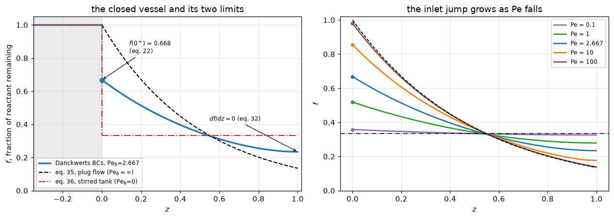
the inlet jump 1 - f(0+), from Wehner & Wilhelm eq. (22):
  Pe =    0.1   f(0+) = 0.3583   jump = 0.6417
  Pe =      1   f(0+) = 0.5189   jump = 0.4811
  Pe =  2.667   f(0+) = 0.6681   jump = 0.3319
  Pe =     10   f(0+) = 0.8541   jump = 0.1459
  Pe =    100   f(0+) = 0.9808   jump = 0.0192
Validation
The checks, in the order docs/agent-brief.md ranks them, each followed by what it cannot see.
1. The closed form, and the observed order
The pymrm solve and Danckwerts’ eq. (34) share nothing but the two parameters: one assembles a finite-volume operator, the other evaluates an exponential expression transcribed from a page image. Refining the grid must drive them together at the scheme’s order: first for bare upwind, second with van Leer. Since eq. (34) is exact, every column below is an error, not a spread.
The table reads the exit two ways. The outlet-face value from compute_boundary_values is what the scheme transported; the last cell centre sits half a cell inside the bed. Because \(\mathrm{d}f/\mathrm{d}z = 0\) at the outlet, the cell-centre read is also second order, so a convergence order cannot tell the two apart, but its error constant is larger.
NS = (25, 50, 100, 200, 400, 800, 1600)


def closed_ladder(ns=NS, Pe=PE_B, R=R_REF, limiter=vanleer, lead=4.0, inlet="danckwerts",
                  second_limiter=None, residual="correction"):
    """Errors against eq. 34 on a grid ladder, with the deferred-correction gap.

    ``limiter`` is the TVD limiter of the Newton route; ``second_limiter`` (default
    the same) is the one handed to the deferred-correction route.
    """
    ref_exit = f_exit_D34(Pe, R, lead)
    up, tv_cell, tv_face, gap = [], [], [], []
    for n in ns:
        m = ClosedVessel(Pe, R, n=n, inlet=inlet)
        up.append(abs(m.solve(limiter=None).c_exit / ref_exit - 1))
        tv = m.solve(limiter=limiter, residual=residual)
        tv_cell.append(abs(tv.c[-1] / ref_exit - 1))
        tv_face.append(abs(tv.c_exit / ref_exit - 1))
        if limiter is not None:
            dc = m.solve_deferred(limiter=second_limiter or limiter, max_it=400)
            gap.append(abs(tv.c_exit - dc.c_exit))
    out = {k: np.array(v) for k, v in
           dict(up=up, tv_cell=tv_cell, tv_face=tv_face, gap=gap or [np.nan]).items()}
    out["order_up"] = float(np.log2(out["up"][-2] / out["up"][-1]))
    out["order_tv"] = float(np.log2(out["tv_face"][-2] / out["tv_face"][-1]))
    out["order_cell"] = float(np.log2(out["tv_cell"][-2] / out["tv_cell"][-1]))
    return out


LAD = closed_ladder()
print(f"{'n':>6} {'upwind':>11} {'order':>6}   {'van Leer, last cell':>19} {'order':>6}"
      f"   {'van Leer, face':>14} {'order':>6}")
for i, n in enumerate(NS):
    o = [np.log2(LAD[k][i - 1] / LAD[k][i]) if i else np.nan
         for k in ("up", "tv_cell", "tv_face")]
    print(f"{n:6d} {LAD['up'][i]:11.3e} {o[0]:6.2f}   {LAD['tv_cell'][i]:19.3e} {o[1]:6.2f}"
          f"   {LAD['tv_face'][i]:14.3e} {o[2]:6.2f}")
ERR_TV, ERR_TV_CELL = float(LAD["tv_face"][-1]), float(LAD["tv_cell"][-1])
GAP_CLOSED = float(np.max(LAD["gap"]))
print(f"\nobserved order on the face: upwind {LAD['order_up']:.2f}, van Leer "
      f"{LAD['order_tv']:.2f} (the last-cell read {LAD['order_cell']:.2f})")
CELL_OVER_FACE = ERR_TV_CELL / ERR_TV
FACE_CLOSER = bool(np.all(LAD["tv_face"] < LAD["tv_cell"]))
BOTH_MONOTONE = bool(np.all(np.diff(LAD["tv_face"]) < 0) and np.all(np.diff(LAD["tv_cell"]) < 0))
print(f"at n = {NS[-1]} the last-cell read is {CELL_OVER_FACE:.1f} times the face error;")
print(f"face read closer than the last-cell read on every rung: {FACE_CLOSER}; both errors")
print(f"decrease monotonically along the ladder: {BOTH_MONOTONE}"
      + ("; so the face value is the more accurate exit, not only a different one."
         if FACE_CLOSER and BOTH_MONOTONE else "."))
print("Newton (ConvFluxTVD) against deferred correction, same discrete equations, worst over")
print(f"the ladder: below 1e-13 (here {GAP_CLOSED:.1e})")
GAP_CLOSED_FULL = float(np.max(closed_ladder(ns=NS[-2:], residual="full")["gap"]))
print("The same with Newton's residual written in full instead of as the correction to the")
print(f"upwind solution (model.py, Notes): below 1e-10 (here {GAP_CLOSED_FULL:.1e}), a state")
print("that also moves with the BLAS kernel; the correction form brings Newton onto the")
print("deferred-correction state.  Both routes share one LU of the upwind operator, so")
print("that agreement says nothing about the factorisation; re-factorised with another")
print("column ordering (permc_spec MMD_ATA):")


def factorisation_spread(ns=(800, 1600), residual="correction"):
    """Largest change of the exit when the upwind operator is factorised differently."""
    out = []
    for n in ns:
        ref_n = ClosedVessel(PE_B, R_REF, n=n).solve()
        alt = ClosedVessel(PE_B, R_REF, n=n, permc_spec="MMD_ATA").solve(residual=residual)
        out.append(abs(alt.c_exit - ref_n.c_exit))
    return float(max(out))


FACT_SPREAD = factorisation_spread()
print(f"  the exit reproduces to below 5e-13 (here {FACT_SPREAD:.1e}) at n = 800 and 1600, which")
print("  is the round-off floor of the exit itself.")
n upwind order van Leer, last cell order van Leer, face order
25 1.141e-02 nan 9.529e-04 nan 6.406e-05 nan
50 5.663e-03 1.01 2.350e-04 2.02 2.528e-05 1.34
100 2.821e-03 1.01 5.804e-05 2.02 7.832e-06 1.69
200 1.407e-03 1.00 1.437e-05 2.01 2.194e-06 1.84
400 7.030e-04 1.00 3.570e-06 2.01 5.841e-07 1.91
800 3.513e-04 1.00 8.889e-07 2.01 1.513e-07 1.95
1600 1.756e-04 1.00 2.217e-07 2.00 3.855e-08 1.97
observed order on the face: upwind 1.00, van Leer 1.97 (the last-cell read 2.00)
at n = 1600 the last-cell read is 5.8 times the face error;
face read closer than the last-cell read on every rung: True; both errors
decrease monotonically along the ladder: True; so the face value is the more accurate exit, not only a different one.
Newton (ConvFluxTVD) against deferred correction, same discrete equations, worst over
the ladder: below 1e-13 (here 6.7e-16)
The same with Newton's residual written in full instead of as the correction to the
upwind solution (model.py, Notes): below 1e-10 (here 1.2e-12), a state
that also moves with the BLAS kernel; the correction form brings Newton onto the
deferred-correction state. Both routes share one LU of the upwind operator, so
that agreement says nothing about the factorisation; re-factorised with another
column ordering (permc_spec MMD_ATA):
the exit reproduces to below 5e-13 (here 1.9e-13) at n = 800 and 1600, which
is the round-off floor of the exit itself.# the upwind error is not just "first order": it has a known mechanism
PE_EFF_NS = (50, 100, 200, 400, 800, 1600)
def pe_eff_residuals(factor=0.5, ns=PE_EFF_NS):
"""Bare upwind against eq. 34 at Pe_eff = 1/(1/Pe + factor*dz), dz = 1/n."""
res = []
for n in ns:
f_up = ClosedVessel(PE_B, R_REF, n=n).solve(limiter=None).c_exit
res.append(abs(f_up / f_exit_D34(1.0 / (1.0 / PE_B + factor / n), R_REF) - 1))
res = np.array(res)
return res, float(np.log2(res[-2] / res[-1]))
PE_EFF_RES, PE_EFF_ORDER = pe_eff_residuals()
print("Upwind adds a numerical diffusivity u*dz/2, which is the same thing as")
print("solving a smaller Peclet number. Comparing against eq. 34 evaluated at")
print("Pe_eff = 1/(1/Pe + dz/2) should therefore leave only a SECOND-order residual:")
for i, n in enumerate(PE_EFF_NS):
o = f" order {np.log2(PE_EFF_RES[i - 1] / PE_EFF_RES[i]):5.2f}" if i else ""
print(f" n={n:5d} residual {PE_EFF_RES[i]:9.3e}" + o)
def pe_eff(Pe, n, factor=0.5):
return 1.0 / (1.0 / Pe + factor / n)
PE_EFF_200 = pe_eff(200.0, 200)
print(f"\nSo a bare-upwind study of inlet conditions at Pe = 200 on a 200-cell grid")
print(f"is really running at Pe_eff = {PE_EFF_200:.0f}, and would be measuring its own")
print("truncation error as though it were a boundary-condition effect.")Upwind adds a numerical diffusivity u*dz/2, which is the same thing as
solving a smaller Peclet number. Comparing against eq. 34 evaluated at
Pe_eff = 1/(1/Pe + dz/2) should therefore leave only a SECOND-order residual:
n= 50 residual 1.179e-04
n= 100 residual 2.983e-05 order 1.98
n= 200 residual 7.499e-06 order 1.99
n= 400 residual 1.880e-06 order 2.00
n= 800 residual 4.707e-07 order 2.00
n= 1600 residual 1.178e-07 order 2.00
So a bare-upwind study of inlet conditions at Pe = 200 on a 200-cell grid
is really running at Pe_eff = 133, and would be measuring its own
truncation error as though it were a boundary-condition effect.What check 1 cannot see. It is one number at one operating point, so it cannot detect a defect that only shows at another \(\mathrm{Pe}\) or \(R\); check 2 sweeps the Peclet number for that reason. It also has weak power against under-resolution here specifically: at \(\mathrm{Pe}_b = 2.667\) the profile is so smooth that a 10-cell grid is already close (see the break table), whereas at \(\mathrm{Pe} = 200\) the same 10 cells are wrong by far more. Grid convergence is reported as a table, not as a single tolerance, for exactly that reason.
2. The two exact limits, and the printed asymptote
Danckwerts’ eqs. (35) and (36) are limits the model must hit, not approximations: \(f \to e^{-R}\) as \(\mathrm{Pe}\to\infty\) and \(f \to 1/(1+R)\) as \(\mathrm{Pe}\to 0\). His eq. (37) claims something sharper, that the approach to plug flow is \(f \approx (1 + R^{2}/\mathrm{Pe})e^{-R}\), which fixes both the sign and the size of the first correction, and can be tested for its order.
PE_SWEEP = np.logspace(-4, 4, 33)


def pe_sweep(n=1600, limiter=vanleer):
    """pymrm against eq. 34 over the sweep: face read and last-cell read."""
    sols = [ClosedVessel(p, R_REF, n=n).solve(limiter=limiter) for p in PE_SWEEP]
    exact = f_exit_D34(PE_SWEEP, R_REF)
    face = np.array([s.c_exit for s in sols])
    cell = np.array([s.c[-1] for s in sols])
    return face, np.abs(face / exact - 1), np.abs(cell / exact - 1)


F_SWEEP, SWEEP_FACE, SWEEP_CELL = pe_sweep()
SWEEP_WORST, SWEEP_WORST_CELL = float(SWEEP_FACE.max()), float(SWEEP_CELL.max())
I_1E4 = int(np.argmin(np.abs(PE_SWEEP - 1e4)))
PE_HI = np.logspace(1, 4.5, 25)


def eq37_residual(Pe, R=R_REF, power=2.0):
    """|eq. 37 / eq. 34 - 1|; power is the exponent of R in the correction term."""
    return np.abs((1 + R ** power / Pe) * np.exp(-R) / f_exit_D34(Pe, R) - 1)


def limit_checks(lead=4.0, power=2.0):
    """eq. 34 against eqs. 35 and 36, and the decay exponent of eq. 37's residual."""
    res = eq37_residual(PE_HI, power=power)
    fit = PE_HI >= 1e3        # the exponent is asymptotic in 1/Pe: fit where 1/Pe is small
    return dict(
        plug=float(abs(f_exit_D34(1e8, R_REF, lead) / np.exp(-R_REF) - 1)),
        cstr=float(abs(f_exit_D34(1e-8, R_REF, lead) / (1 / (1 + R_REF)) - 1)),
        order=float(-np.polyfit(np.log(PE_HI[fit]), np.log(res[fit]), 1)[0]),
        order_all=float(-np.polyfit(np.log(PE_HI), np.log(res), 1)[0]),
        dev100=float(eq37_residual(100.0, power=power)), res=res, fit=fit)


LIM = limit_checks()

fig, axes = plt.subplots(1, 2, figsize=(11.6, 4.0))
ax = axes[0]
ax.semilogx(PE_SWEEP, f_exit_D34(PE_SWEEP, R_REF), "k-", lw=1.6, label="eq. 34")
ax.semilogx(PE_SWEEP, F_SWEEP, "o", ms=4, mfc="none", color="tab:blue", label="pymrm")
ax.axhline(np.exp(-R_REF), color="tab:green", ls="--", lw=1.2,
           label=fr"eq. 35, $e^{{-R}}$ = {np.exp(-R_REF):.4f}")
ax.axhline(1 / (1 + R_REF), color="tab:red", ls="-.", lw=1.2,
           label=fr"eq. 36, $1/(1+R)$ = {1/(1+R_REF):.4f}")
ax.set(xlabel="Pe", ylabel="$f$ at the exit", title=f"the Peclet sweep, R = {R_REF:g}")
ax.legend(fontsize=8)

ax = axes[1]
ax.loglog(PE_HI, LIM["res"], "o-", ms=4, color="tab:blue", label="| eq. 37 / eq. 34  - 1 |")
ax.loglog(PE_HI[LIM["fit"]], LIM["res"][LIM["fit"]], "o", ms=7, mfc="none", color="tab:red",
          label="fitted for the exponent")
ax.loglog(PE_HI, LIM["res"][0] * (PE_HI / PE_HI[0]) ** -2.0, "k--", lw=1.0, label=r"slope $-2$")
ax.set(xlabel="Pe", ylabel="relative residual of eq. 37",
       title="eq. 37 is exact to first order in 1/Pe")
ax.legend(fontsize=8)
fig.tight_layout()
plt.show()

print(f"pymrm vs eq. 34 over Pe = {PE_SWEEP[0]:g} .. {PE_SWEEP[-1]:g} "
      f"({np.log10(PE_SWEEP[-1] / PE_SWEEP[0]):.0f} decades, {PE_SWEEP.size} values), "
      f"n = 1600:")
print(f"  outlet face      : worst {SWEEP_WORST:.2e}; at Pe = 1e4 {SWEEP_FACE[I_1E4]:.2e}")
print(f"  last cell centre : worst {SWEEP_WORST_CELL:.2e}; at Pe = 1e4 {SWEEP_CELL[I_1E4]:.2e}")
print("At high Pe the outlet carries a boundary layer of width 1/Pe, far thinner than a")
print("cell. The solve's exit, on the face, agrees with eq. 34; the last-cell number is")
print("the distance of the last cell value from the exit, which is large because the")
print("outlet layer is thinner than a cell (the break table halves the grid and that")
print("distance roughly doubles).")
print(f"eq. 34 -> eq. 35 (plug)  at Pe = 1e8  : {LIM['plug']:.2e}")
print(f"eq. 34 -> eq. 36 (CSTR)  at Pe = 1e-8 : {LIM['cstr']:.2e}")
print(f"eq. 37 residual decays as Pe^-{LIM['order']:.2f}, fitted over the asymptotic end")
print(f"  Pe >= 1e3 ({LIM['fit'].sum()} points); the R^2/Pe term is therefore the exact first")
print("  correction, with the next one down at 1/Pe^2.  Fitting the whole plotted")
print(f"  range instead returns {LIM['order_all']:.2f}, which is not a second exponent but the")
print("  pre-asymptotic bottom end leaking in, where R^2/Pe is not small.")
print(f"At Pe = 100 the approximation is {100 * LIM['dev100']:.3f} % high.")
print("His own criterion k^2 D L/u^3 = R^2/Pe < 1 is met once Pe exceeds R^2.")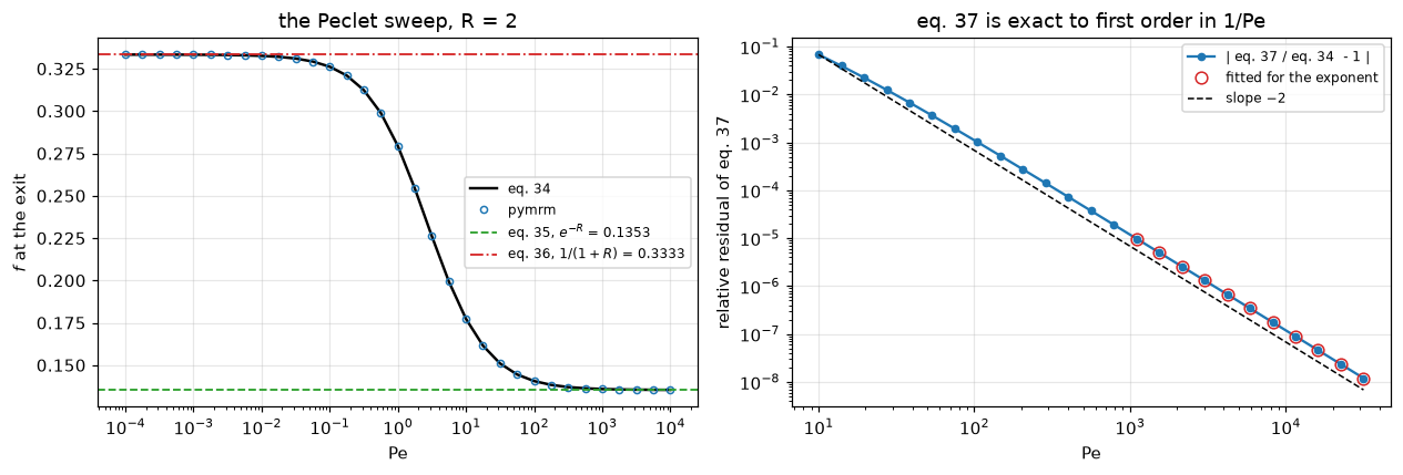
pymrm vs eq. 34 over Pe = 0.0001 .. 10000 (8 decades, 33 values), n = 1600:
  outlet face      : worst 3.62e-07; at Pe = 1e4 6.18e-08
  last cell centre : worst 1.88e-04; at Pe = 1e4 1.88e-04
At high Pe the outlet carries a boundary layer of width 1/Pe, far thinner than a
cell. The solve's exit, on the face, agrees with eq. 34; the last-cell number is
the distance of the last cell value from the exit, which is large because the
outlet layer is thinner than a cell (the break table halves the grid and that
distance roughly doubles).
eq. 34 -> eq. 35 (plug)  at Pe = 1e8  : 4.55e-08
eq. 34 -> eq. 36 (CSTR)  at Pe = 1e-8 : 2.22e-09
eq. 37 residual decays as Pe^-2.00, fitted over the asymptotic end
  Pe >= 1e3 (11 points); the R^2/Pe term is therefore the exact first
  correction, with the next one down at 1/Pe^2.  Fitting the whole plotted
  range instead returns 1.95, which is not a second exponent but the
  pre-asymptotic bottom end leaking in, where R^2/Pe is not small.
At Pe = 100 the approximation is 0.112 % high.
His own criterion k^2 D L/u^3 = R^2/Pe < 1 is met once Pe exceeds R^2.
What check 2 cannot see. The two limits are limits of the closed form, so they test the transcription, not the modelling choice; and both limits are reached by any reasonable pair of boundary conditions at \(\mathrm{Pe}\to\infty\) (convection swamps everything). Only the \(\mathrm{Pe}\to 0\) limit discriminates between inlet conditions, which is precisely Wehner & Wilhelm’s objection to Hulburt, and check 5 turns it into a number.
3. Wehner & Wilhelm’s three sections, a route that never writes a Danckwerts condition
This is the check with the most power, because it obtains the same profile from a different problem statement, though, to be precise about what that buys, not from different code: it shares construct_grad, construct_div, construct_convflux_upwind, ConvFluxTVD and the solver with ClosedVessel, and its condition at \(z = 1\) is close to the closed vessel’s without being the same: both carry zero diffusive flux there, but the closed vessel’s outlet face carries the value reconstructed from the zero-gradient dictionary, \((9c_N - c_{N-1})/8\), while the three-section bed exit carries \(c_N\) (measured in the gradient cell below). What it genuinely establishes is that Danckwerts’ closure is the right reduction of the three-section problem (it separates his solution from Hulburt’s by 50 % at the reference point) and that the reaction section is invariant to both end sections.
ThreeSection in model.py runs the domain from far upstream to far downstream in one grid, with a piecewise diffusivity (\(1/\mathrm{Pe}_a\), \(1/\mathrm{Pe}_b\), \(1/\mathrm{Pe}_c\)) and reaction only inside \(0<z<1\). The only boundary conditions imposed are Wehner & Wilhelm’s own eqs. (8) and (15): \(f = 1\) far upstream, and \(f\) finite far downstream, which for a section with no reaction is rendered exactly by a zero gradient at the truncation. Nothing is imposed at \(z=0\) or \(z=1\): the interfaces are ordinary interior faces where the finite-volume scheme enforces continuity of \(f\) and of the total flux, which are their eqs. (11) to (14). The face diffusivities enter through construct_coefficient_matrix.
At a jump in \(D\) the face diffusivity must be the harmonic mean of the two neighbouring cell values, because that is what keeps the diffusive flux continuous when the profile has a kink. The arithmetic mean leaves an \(O(1)\) flux error at that one face, and the cost is an order, not a factor: the study below refines the bed and reports both convergence rates, because a single “\(N\times\) worse” number is a property of the grid it was measured on.
TS_CASES = [(0.01, 1.0), (0.1, 1.0), (1.0, 1.0), (10.0, 1.0), (1000.0, 1.0),
            (1.0, 0.01), (1.0, 100.0)]


def ts_sweep(n_b=400, P=30.0, deferred_tol=1e-11):
    """The three-section problem over Pe_a and Pe_c, on stretched end sections."""
    rows = []
    for Pe_a, Pe_c in TS_CASES:
        m = ThreeSection(Pe_a, PE_B, Pe_c, R_REF, n_b=n_b, P=P)
        zc, cc, _, _ = m.solve()
        _, cd = ThreeSection(Pe_a, PE_B, Pe_c, R_REF, n_b=n_b, P=P).solve_deferred(
            tol=deferred_tol, max_it=400)
        bed = (zc > 0) & (zc < 1.0)
        rows.append((float(np.max(np.abs(cc[bed] - c_prof_D33(zc[bed], PE_B, R_REF)))),
                     float(abs(m.exit_value(cc) / f_exit_W21(PE_B, R_REF) - 1)),
                     float(np.max(np.abs(cc - cd)))))
    return np.array(rows)


TS = ts_sweep()
TS_DEV, TS_SPREAD, TS_GAP = float(TS[:, 0].max()), float(np.ptp(TS[:, 1])), float(TS[:, 2].max())
print("Wehner & Wilhelm's claim: the reaction section does not depend on either")
print("end section.  Sweeping Pe_a and Pe_c:\n")
print(f"{'Pe_a':>9} {'Pe_c':>9} {'max|f - eq.33| in bed':>23} {'f(exit) vs eq.21':>18}")
for (Pe_a, Pe_c), (dev, ex, _) in zip(TS_CASES, TS):
    print(f"{Pe_a:9.2f} {Pe_c:9.2f} {dev:23.3e} {ex:18.3e}")
print(f"\nworst deviation from the closed vessel, over all {len(TS_CASES)} runs: {TS_DEV:.2e}")
print(f"spread of f(exit) across them:                              {TS_SPREAD:.2e}")
print("Newton against deferred correction on the same grids, largest cell difference:")
print(f"  below 1e-9 (here {TS_GAP:.1e})")
print("The reaction section is blind to both end sections, as they claim, and the")
print("Danckwerts conditions are what a solve that never mentions them produces.")
Wehner & Wilhelm's claim: the reaction section does not depend on either
end section. Sweeping Pe_a and Pe_c:
Pe_a Pe_c max|f - eq.33| in bed f(exit) vs eq.21
0.01 1.00 1.921e-06 8.114e-07
0.10 1.00 1.824e-06 8.109e-07
1.00 1.00 8.502e-07 8.061e-07
10.00 1.00 3.493e-06 7.842e-07
1000.00 1.00 7.828e-06 7.618e-07
1.00 0.01 8.502e-07 8.060e-07
1.00 100.00 8.502e-07 8.061e-07
worst deviation from the closed vessel, over all 7 runs: 7.83e-06
spread of f(exit) across them: 4.96e-08
Newton against deferred correction on the same grids, largest cell difference:
below 1e-9 (here 1.2e-11)
The reaction section is blind to both end sections, as they claim, and the
Danckwerts conditions are what a solve that never mentions them produces.# the full three-section profile, on uniform grids, against eqs. 19 to 22
def ts_profile(P=20.0, n_b=400, limiter=vanleer, a_in_exp=True, react_past_bed=False):
"""Deviations of the uniform-grid three-section solve from eqs. 19 to 21."""
m = ThreeSection(PE_A, PE_B, 1.0, R_REF, n_b=n_b, stretch=False, P=P,
react_past_bed=react_past_bed)
zc, cc, zf, fl = m.solve(limiter=limiter)
m_f, m_b, m_a = zc < 0, (zc > 0) & (zc < 1.0), zc > 1.0
f0 = f0_W22(PE_B, R_REF, a_in_exp)
eq19 = 1.0 - (1.0 - f0) * np.exp(PE_A * zc[m_f])
return dict(zc=zc, cc=cc, m_f=m_f, m_b=m_b, eq19=eq19,
fore=float(np.max(np.abs(cc[m_f] - eq19))),
bed=float(np.max(np.abs(cc[m_b] - c_prof_D33(zc[m_b], PE_B, R_REF)))),
exit=float(abs(m.exit_value(cc) / f_exit_W21(PE_B, R_REF) - 1)),
flat=float(np.ptp(cc[m_a])),
flux=float(np.max(np.abs(fl[zf < 0] - 1.0))),
flux_est=float((1.0 - f0) * np.exp(-P)), n_after=int(m_a.sum()), n=m.n)
TP = ts_profile()
fig, axes = plt.subplots(1, 2, figsize=(11.6, 4.2))
ax = axes[0]
for Pe_a, col in [(0.3, "tab:purple"), (1.0, "tab:blue"), (3.0, "tab:orange"),
(30.0, "tab:green")]:
z2, c2, _, _ = ThreeSection(Pe_a, PE_B, 1.0, R_REF).solve()
k = (z2 > -3.5) & (z2 < 2.5)
ax.plot(z2[k], c2[k], color=col, lw=1.7, label=f"Pe$_a$ = {Pe_a:g}")
ax.plot(ZZ, c_prof_D33(ZZ, PE_B, R_REF), "k--", lw=2.4, alpha=0.6, label="Danckwerts eq. 33")
ax.axvspan(0, 1, color="0.93")
ax.text(0.5, 0.05, "reaction section", ha="center", fontsize=8)
ax.set(xlabel="$z$", ylabel="$f$", xlim=(-3.5, 2.5), ylim=(0, 1.05),
title="the bed profile ignores the fore section")
ax.legend(fontsize=8, loc="lower left")
ax = axes[1]
zc, cc, m_f = TP["zc"], TP["cc"], TP["m_f"]
k = (zc > -6) & (zc < 3)
ax.plot(zc[k], cc[k], color="tab:blue", lw=2.0, label="pymrm, three sections")
ax.plot(zc[m_f][zc[m_f] > -6], TP["eq19"][zc[m_f] > -6], "r:", lw=1.6, label="W&W eq. 19")
ax.plot(ZZ, c_prof_D33(ZZ, PE_B, R_REF), "k--", lw=1.6, label="W&W eq. 20 = D. eq. 33")
ax.axhline(f_exit_W21(PE_B, R_REF), color="tab:green", ls="-.", lw=1.4, label="W&W eq. 21")
ax.plot(0.0, f0_W22(PE_B, R_REF), "o", color="k", ms=6)
ax.annotate("W&W eq. 22", xy=(0.0, f0_W22(PE_B, R_REF)), xytext=(0.35, 0.85),
fontsize=8, arrowprops=dict(arrowstyle="->", lw=0.8))
ax.axvspan(0, 1, color="0.93")
ax.set(xlabel="$z$", ylabel="$f$", ylim=(0, 1.05),
title=fr"all three sections, Pe$_a$ = {PE_A:g}, Pe$_b$ = {PE_B:g}")
ax.legend(fontsize=8, loc="lower left")
fig.tight_layout()
plt.show()
print(f"fore section vs W&W eq. 19 : max |deviation| {TP['fore']:.2e}")
print(f"reaction sect. vs W&W eq. 20 : max |deviation| {TP['bed']:.2e}")
print(f"exit value vs W&W eq. 21 : relative {TP['exit']:.2e}")
print(" those three are measurements: each has a closed form it could disagree")
print(" with, and the arithmetic-mean run below shows the first one moving.")
print()
print(f"fore-section flux, max |F - 1| below 1e-8 (here {TP['flux']:.1e}); the truncation estimate")
print(f" (1 - f(0)) exp(-P) = {TP['flux_est']:.1e} for an upstream section of P = 20 decay lengths.")
print(" With no source upstream the discrete divergence is zero cell by cell, so the")
print(" fore flux is constant by construction; its VALUE is a check that the upstream")
print(" domain is long enough: the truncation error, plus the round-off floor of this")
print(f" {TP['n']}-cell uniform grid, which is of the same size here.")
print(f"after section flat? peak-to-peak below 1e-9 (here {TP['flat']:.1e})")
print(" For this model it is an identity of the discrete equations: downstream the flux")
print(" balance with no reaction and constant D forces c_i = c_(i+1), for ANY Pe_c and")
print(" ANY truncation length, so the peak-to-peak above is round-off. It is not")
print(" structural: let the reaction run on past z = 1 and it fails (break table).")
print(f" Measured, against the 20-decay-length, {TP['n_after']}-cell after section that")
print(" produced the number above:")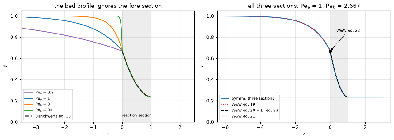
fore section   vs W&W eq. 19 : max |deviation| 9.03e-07
reaction sect. vs W&W eq. 20 : max |deviation| 8.48e-07
exit value     vs W&W eq. 21 : relative        8.08e-07
  those three are measurements: each has a closed form it could disagree
  with, and the arithmetic-mean run below shows the first one moving.

fore-section flux, max |F - 1| below 1e-8 (here 1.2e-09); the truncation estimate
  (1 - f(0)) exp(-P) = 6.8e-10 for an upstream section of P = 20 decay lengths.
  With no source upstream the discrete divergence is zero cell by cell, so the
  fore flux is constant by construction; its VALUE is a check that the upstream
  domain is long enough: the truncation error, plus the round-off floor of this
  16400-cell uniform grid, which is of the same size here.
after section flat? peak-to-peak below 1e-9 (here 8.2e-11)
  For this model it is an identity of the discrete equations: downstream the flux
  balance with no reaction and constant D forces c_i = c_(i+1), for ANY Pe_c and
  ANY truncation length, so the peak-to-peak above is round-off.  It is not
  structural: let the reaction run on past z = 1 and it fails (break table).
  Measured, against the 20-decay-length, 8000-cell after section that
  produced the number above:
# is "the after section is flat" a measurement or an identity? Truncate it.
# Everything else (Pe_a, Pe_b, Pe_c, the bed grid, the fore section) is held
# at the values that produced the 20-decay-length numbers printed above.
def truncation_study(react_past_bed=False, verbose=False):
"""After-section flatness and bed change when the after section is cut short."""
base = ts_profile(react_past_bed=react_past_bed)
flat, bed = [], []
for P_after in (2.0, 0.2):
z3, c3, _, _ = ThreeSection(PE_A, PE_B, 1.0, R_REF, stretch=False, P=20.0,
P_after=P_after, react_past_bed=react_past_bed).solve()
ma3, mb3 = z3 > 1.0, (z3 > 0) & (z3 < 1.0)
flat.append(float(np.ptp(c3[ma3])))
bed.append(float(np.max(np.abs(c3[mb3] - base["cc"][base["m_b"]]))))
if verbose:
print(f" after section {P_after:5g} decay lengths ({ma3.sum():5d} cells): "
f"peak-to-peak below 1e-9 (here {flat[-1]:.1e})")
print(f" bed profile unchanged: below 1e-9 (here {bed[-1]:.1e})")
return max(flat), max(bed)
TRUNC_FLAT, TRUNC_BED = truncation_study(verbose=True)
print("An after section 100x too short reads as flat just as convincingly, and the")
print("bed does not notice, so flatness is evidence about the DISCRETISATION, not")
print("about Pe_c or the truncation length. What it does license is the argument")
print("below: flat implies zero diffusive flux at z = 1.") after section 2 decay lengths ( 800 cells): peak-to-peak below 1e-9 (here 1.7e-12)
bed profile unchanged: below 1e-9 (here 3.2e-13)
after section 0.2 decay lengths ( 80 cells): peak-to-peak below 1e-9 (here 2.8e-14)
bed profile unchanged: below 1e-9 (here 3.0e-13)
An after section 100x too short reads as flat just as convincingly, and the
bed does not notice, so flatness is evidence about the DISCRETISATION, not
about Pe_c or the truncation length. What it does license is the argument
below: flat implies zero diffusive flux at z = 1.What the arithmetic face average would have cost, and why no single factor should be quoted. Re-running the same problem with \(D\) averaged arithmetically at the two jumps, refining only the bed:
N_BED = (100, 200, 400, 800)


def face_ladder(pair=("arithmetic", "harmonic"), n_bed=N_BED):
    """Fore-section error against eq. 19 for two face averages, refining the bed."""
    err = {0: [], 1: []}
    for n_b in n_bed:
        for j, fa in enumerate(pair):
            m = ThreeSection(PE_A, PE_B, 1.0, R_REF, n_b=n_b, stretch=False, P=20.0,
                             face_average=fa)
            z4, c4, _, _ = m.solve()
            m4 = z4 < 0
            eq19 = 1.0 - (1.0 - f0_W22(PE_B, R_REF)) * np.exp(PE_A * z4[m4])
            err[j].append(float(np.max(np.abs(c4[m4] - eq19))))
    a, h = np.array(err[0]), np.array(err[1])
    return dict(a=a, h=h, ratio=a / h, order_a=float(np.log2(a[-2] / a[-1])),
                order_h=float(np.log2(h[-2] / h[-1])))


FL = face_ladder()
print(f"{'n_b':>6} {'arithmetic':>12} {'order':>7} {'harmonic':>12} {'order':>7} {'ratio':>7}")
for i, n_b in enumerate(N_BED):
    o_a = np.log2(FL["a"][i - 1] / FL["a"][i]) if i else np.nan
    o_h = np.log2(FL["h"][i - 1] / FL["h"][i]) if i else np.nan
    mark = "   <- this page's grid" if n_b == 400 else ""
    shown = f"{round(FL['ratio'][i], -1):.0f}" if n_b == N_BED[-1] else f"{FL['ratio'][i]:.0f}"
    if n_b == N_BED[-1]:
        mark = "   <- about; round-off on this grid leaves the last digit unresolved"
    print(f"{n_b:6d} {FL['a'][i]:12.3e} {o_a:7.2f} {FL['h'][i]:12.3e} {o_h:7.2f} "
          f"{shown:>7}{mark}")
I400 = N_BED.index(400)
print(f"\nThe arithmetic mean converges at order {FL['order_a']:.2f} at the jump, the harmonic")
print(f"at order {FL['order_h']:.2f}, so the ratio is not a constant: it grows in proportion")
print(f"to n, without bound.  The {FL['ratio'][I400]:.0f}x on this page's n_b = 400 grid is "
      f"{FL['ratio'][0]:.0f}x on a")
print(f"{N_BED[0]}-cell bed and about {round(FL['ratio'][-1], -1):.0f}x on an {N_BED[-1]}-cell one.  "
      "Quote the ORDER: a lone factor")
print("is a property of the grid it was measured on, and on a coarse grid it looks")
print("small enough to dismiss the rule.")


def silent_failure(n_b=400):
    """What a reader sees with each face average: first bed cell, exit, bed error."""
    out = {}
    for fa in ("harmonic", "arithmetic"):
        m = ThreeSection(PE_A, PE_B, 1.0, R_REF, n_b=n_b, stretch=False, P=20.0,
                         face_average=fa)
        z5, c5, _, _ = m.solve()
        mb5 = (z5 > 0) & (z5 < 1.0)
        out[fa] = (float(c5[mb5][0]), m.exit_value(c5),
                   float(np.max(np.abs(c5[mb5] - c_prof_D33(z5[mb5], PE_B, R_REF)))))
    out["first_shift"] = abs(out["arithmetic"][0] - out["harmonic"][0])
    out["exit_shift"] = abs(out["arithmetic"][1] - out["harmonic"][1])
    return out


SF = silent_failure()
print()
print("And it fails SILENTLY.  Same two runs at n_b = 400, looking at what a reader")
print("would actually see:")
for fa in ("harmonic", "arithmetic"):
    print(f"  {fa:>10}: f in the first bed cell {SF[fa][0]:.6f}, "
          f"f(exit) {SF[fa][1]:.8f}, bed vs eq. 33 {SF[fa][2]:.1e}")
print(f"  the exit value moves by {SF['exit_shift']:.1e} and the profile stays smooth and")
print("  plausible: nothing downstream of the jump reports the error.  The damage")
print("  is real but LOCAL: it is the fore section, not the answer, that is wrong.")
n_b arithmetic order harmonic order ratio
100 1.241e-03 nan 1.471e-05 nan 84
200 6.248e-04 0.99 3.632e-06 2.02 172
400 3.134e-04 1.00 9.029e-07 2.01 347 <- this page's grid
800 1.569e-04 1.00 2.252e-07 2.00 700 <- about; round-off on this grid leaves the last digit unresolved
The arithmetic mean converges at order 1.00 at the jump, the harmonic
at order 2.00, so the ratio is not a constant: it grows in proportion
to n, without bound. The 347x on this page's n_b = 400 grid is 84x on a
100-cell bed and about 700x on an 800-cell one. Quote the ORDER: a lone factor
is a property of the grid it was measured on, and on a coarse grid it looks
small enough to dismiss the rule.
And it fails SILENTLY. Same two runs at n_b = 400, looking at what a reader
would actually see:
harmonic: f in the first bed cell 0.667012, f(exit) 0.23442834, bed vs eq. 33 8.5e-07
arithmetic: f in the first bed cell 0.667011, f(exit) 0.23442834, bed vs eq. 33 1.6e-06
the exit value moves by 9.3e-10 and the profile stays smooth and
plausible: nothing downstream of the jump reports the error. The damage
is real but LOCAL: it is the fore section, not the answer, that is wrong.Danckwerts’ intuition, recovered. Nothing in the three-section solve imposes \(\mathrm{d}f/\mathrm{d}z = 0\) at \(z=1\). It comes out, because the after section has no reaction and must stay bounded, so it is flat, so continuity of flux drags the zero gradient back to the bed exit: Wehner & Wilhelm’s “the boundary condition at \(z = +\infty\) is drawn to the end of the reaction bed.”
Two things have to be separated here, and the cell below separates them.
- The chain itself is exact in the discrete system. Flat after section means the last bed cell and the first after-section cell hold the same value, so the diffusive flux across \(z=1\) is identically zero. That is measured below and it is at machine precision: nothing about it converges. The zero diffusive flux is what the closed vessel’s
bc_out = {a:1, b:0, d:0}imposes too; the convective flux differs, because the closed vessel’s outlet face carries the value reconstructed from the dictionary and the bed exit here carries the last bed cell. The cell below measures that difference. - Reading a gradient back off cell-centre values is a lossy estimator. The 3-point quadratic fit used below returns a small non-zero number even when it is fed the exact eq. 33, whose gradient at \(z=1\) is exactly zero. So the same fit is applied to the closed form on the same cell centres, and both columns are printed. Most of what the estimator returns is its own truncation error; the part that belongs to the solution is the difference.
N_GRAD = (100, 200, 400, 800)


def grad_study(n_bs=N_GRAD, limiter=vanleer, shift=0, react_past_bed=False):
    """The gradient at z = 1 by a fit of the last three bed cells, on the solve and on eq. 33.

    ``shift`` moves the three-cell window downstream; it exists for the break table.
    """
    g_solve, g_bias, g_resid, gaps = [], [], [], []
    for n_b in n_bs:
        zc2, cc2, _, _ = ThreeSection(PE_A, PE_B, 1.0, R_REF, n_b=n_b,
                                      react_past_bed=react_past_bed).solve(limiter=limiter)
        m = (zc2 > 0) & (zc2 < 1.0)
        last = int(np.flatnonzero(m)[-1]) + shift
        zb, cb = zc2[last - 2:last + 1], cc2[last - 2:last + 1]
        g1 = float(np.polyval(np.polyder(np.polyfit(zb, cb, 2)), 1.0))
        ge = float(np.polyval(np.polyder(np.polyfit(zb, c_prof_D33(zb, PE_B, R_REF), 2)), 1.0))
        g_solve.append(g1)
        g_bias.append(ge)
        g_resid.append(g1 - ge)
        gaps.append(float(abs(cc2[m][-1] - cc2[zc2 > 1.0][0])))
    g_solve, g_bias, g_resid = map(np.array, (g_solve, g_bias, g_resid))
    return dict(solve=g_solve, bias=g_bias, resid=g_resid, gap=float(max(gaps)),
                share=float(abs(g_bias[-1] / g_solve[-1])),
                order=float(np.log2(abs(g_resid[-2] / g_resid[-1]))))


GS = grad_study()
print("gradient at z = 1 recovered from the three-section solve (never imposed there),")
print("beside the SAME 3-point fit applied to the exact eq. 33, whose true gradient")
print("at z = 1 is zero:\n")
print(f"{'n_b':>6} {'fit on the solve':>18} {'fit on exact eq.33':>20} {'difference':>13}")
for i, n_b in enumerate(N_GRAD):
    print(f"{n_b:6d} {GS['solve'][i]:18.4e} {GS['bias'][i]:20.4e} {GS['resid'][i]:13.3e}")
print(f"\n{100 * GS['share']:.0f} % of the recovered gradient is the estimator, not the solution:")
print("the same fit on the exact closed form returns nearly the same number.  What")
print(f"is left after subtracting it falls at order {GS['order']:.2f}, so the conclusion holds,")
print("but the printed magnitude is a post-processing artefact and should not be")
print("read as a physical gradient.")
print()
print("The real content: over every n_b above, the last bed cell and the first")
print(f"after-section cell agree to below 1e-13 (here {GS['gap']:.1e}), so the chain")
print("'after section flat => zero diffusive flux at z = 1' is EXACT in the discrete")
print("system, not second-order.  It is the zero diffusive flux that the closed vessel's")
print("bc_out = {a: 1, b: 0, d: 0} imposes; the convective flux is not identical.  The")
print("closed vessel's outlet face carries (9 c_N - c_(N-1))/8, reconstructed from the")
print("dictionary, while the three-section bed exit carries c_N:")


def outlet_face_vs_last_cell(n=800):
    s_n = ClosedVessel(PE_B, R_REF, n=n).solve()
    return abs(s_n.c_exit - s_n.c[-1]) / s_n.c_exit, s_n


OUTLET_FACE_GAP, _s800 = outlet_face_vs_last_cell()
print(f"  closed vessel, n = 800: outlet flux u f_face = {_s800.c_exit:.8f} against "
      f"u c_N = {_s800.c[-1]:.8f},")
print(f"  {OUTLET_FACE_GAP:.1e} relative; the two closures agree to second order, not exactly.")
print()
print("Honest limit of this check: imposing boundedness at the far downstream")
print("truncation is itself a zero-gradient condition, applied one section away.")
print("What is demonstrated is the chain from f(+inf) finite to df/dz(1)=0, which")
print("is Wehner & Wilhelm's argument, not an independent proof of its premise.")
gradient at z = 1 recovered from the three-section solve (never imposed there),
beside the SAME 3-point fit applied to the exact eq. 33, whose true gradient
at z = 1 is zero:
n_b fit on the solve fit on exact eq.33 difference
100 -3.6404e-04 -3.0440e-04 -5.965e-05
200 -9.2742e-05 -7.7977e-05 -1.477e-05
400 -2.3403e-05 -1.9733e-05 -3.670e-06
800 -5.8782e-06 -4.9634e-06 -9.148e-07
84 % of the recovered gradient is the estimator, not the solution:
the same fit on the exact closed form returns nearly the same number. What
is left after subtracting it falls at order 2.00, so the conclusion holds,
but the printed magnitude is a post-processing artefact and should not be
read as a physical gradient.
The real content: over every n_b above, the last bed cell and the first
after-section cell agree to below 1e-13 (here 5.3e-16), so the chain
'after section flat => zero diffusive flux at z = 1' is EXACT in the discrete
system, not second-order. It is the zero diffusive flux that the closed vessel's
bc_out = {a: 1, b: 0, d: 0} imposes; the convective flux is not identical. The
closed vessel's outlet face carries (9 c_N - c_(N-1))/8, reconstructed from the
dictionary, while the three-section bed exit carries c_N:
closed vessel, n = 800: outlet flux u f_face = 0.23442812 against u c_N = 0.23442836,
1.0e-06 relative; the two closures agree to second order, not exactly.
Honest limit of this check: imposing boundedness at the far downstream
truncation is itself a zero-gradient condition, applied one section away.
What is demonstrated is the chain from f(+inf) finite to df/dz(1)=0, which
is Wehner & Wilhelm's argument, not an independent proof of its premise.And the other Danckwerts condition, qualified by the same model. Wehner & Wilhelm wrote of the inlet discontinuity that it “will be shown later to be not necessarily correct”. Here is what they meant, measured: in the three-section problem \(f\) is continuous at \(z = 0\), and the fall from 1 to \(f(0)\) is spread over the fore section on the scale \(1/\mathrm{Pe}_a\). The mesh resolves it, so what the solve shows at the entrance is a kink in slope, not a jump, and it only becomes Danckwerts’ step in the limit \(\mathrm{Pe}_a\to\infty\).
PE_A_STEPS = (0.3, 1.0, 3.0, 30.0, 1000.0)


def inlet_steps(n_b=200):
    """Adjacent-cell difference across z = 0, and the first bed cell, over Pe_a."""
    jumps, f0_in, rows = [], [], []
    for Pe_a in PE_A_STEPS:
        z6, c6, _, _ = ThreeSection(Pe_a, PE_B, 1.0, R_REF, n_b=n_b).solve()
        i = int(np.searchsorted(z6, 0.0))          # first cell centre inside the bed
        jumps.append(float(c6[i - 1] - c6[i]))
        f0_in.append(float(c6[i]))
        rows.append((Pe_a, float(c6[i - 1]), float(c6[i])))
    return np.array(jumps), float(np.ptp(f0_in)), rows


JUMPS, F0_SPREAD, STEP_ROWS = inlet_steps()
STEP_RATIO = INLET_STEP / JUMPS[1]
print("adjacent-cell difference across z = 0 in the three-section solve, n_b = 200")
print(f"(the closed-vessel idealisation puts a full {INLET_STEP:.3f} step there):\n")
print(f"{'Pe_a':>10} {'f(0-)':>10} {'f(0+)':>10} {'f(0-) - f(0+)':>16}")
for (Pe_a, fm, fp), j in zip(STEP_ROWS, JUMPS):
    print(f"{Pe_a:10g} {fm:10.6f} {fp:10.6f} {j:16.2e}")
print(f"\nAt Pe_a = 1 the entire cell-to-cell change is {JUMPS[1]:.1e}, against a")
print(f"closed-vessel step of {INLET_STEP:.3f}, a factor {STEP_RATIO:.0f} apart.  "
      f"By Pe_a = {PE_A_STEPS[-1]:g} it")
print(f"has grown to {JUMPS[-1]:.1e} and is on its way to the full step.")
print("So Danckwerts' discontinuity is the Pe_a -> infinity idealisation of a")
print("continuous profile, exactly as Wehner & Wilhelm say.  It remains the correct")
print("closure for the bed either way, and the reason is the first bed cell above:")
print(f"f(0+) moves by only {F0_SPREAD:.1e} across that range of Pe_a, so what")
print("the bed sees is the same whatever the fore section does.")
adjacent-cell difference across z = 0 in the three-section solve, n_b = 200
(the closed-vessel idealisation puts a full 0.332 step there):
Pe_a f(0-) f(0+) f(0-) - f(0+)
0.3 0.668344 0.665903 2.44e-03
1 0.668870 0.665906 2.96e-03
3 0.670518 0.665912 4.61e-03
30 0.691585 0.665932 2.57e-02
1000 0.932288 0.665940 2.66e-01
At Pe_a = 1 the entire cell-to-cell change is 3.0e-03, against a
closed-vessel step of 0.332, a factor 112 apart. By Pe_a = 1000 it
has grown to 2.7e-01 and is on its way to the full step.
So Danckwerts' discontinuity is the Pe_a -> infinity idealisation of a
continuous profile, exactly as Wehner & Wilhelm say. It remains the correct
closure for the bed either way, and the reason is the first bed cell above:
f(0+) moves by only 3.7e-05 across that range of Pe_a, so what
the bed sees is the same whatever the fore section does.4. Breaking it on purpose
Every check above is worth exactly what it costs to break. The reference solve is run again with one implementation error injected at a time, and the deviation from eq. (34) recorded. Anything that does not move the number is a blind spot, and is named as one. (The full defect-injection table, which breaks every claim on the page, is under “Claims” below; this one is about the boundary conditions.)
D_REF = 1.0 / PE_B
DEFECTS = [
    ("none (the model as published)", {}),
    ("inlet BC: sign of a flipped (outward normal)", dict(inlet_a=-D_REF)),
    ("inlet BC: naive Dirichlet c(0) = c*", dict(inlet="dirichlet")),
    ("inlet BC: a = D but D taken as 1, not 1/Pe", dict(inlet_a=1.0)),
    ("outlet BC: sign of a flipped", dict(outlet_a=-1.0)),
    ("outlet BC: Dirichlet c(L) = 0", dict(outlet="dirichlet-zero")),
    ("construct_div nu = 1 (cylindrical, wrong)", dict(nu=1)),
    ("reaction term sign flipped", dict(r_sign=-1.0)),
    ("grid coarsened to n = 10", dict(n=10)),
    ("upwind only, no TVD", dict(limiter=None)),
]


def defect_deviation(kw, Pe=PE_B, lead=4.0):
    """Relative deviation of f(exit) from eq. 34 with one defect injected."""
    kw = dict(kw)
    limiter = kw.pop("limiter", vanleer)
    s = ClosedVessel(Pe, R_REF, **{"n": 800, **kw}).solve(limiter=limiter)
    return s.c_exit, float(abs(s.c_exit / f_exit_D34(Pe, R_REF, lead) - 1))


print(f"{'injected defect':>46} {'f(exit)':>11} {'rel. dev. from eq. 34':>22}")
BREAK_TAB = {}
for label, kw in DEFECTS:
    f_d, BREAK_TAB[label] = defect_deviation(kw)
    print(f"{label:>46} {f_d:11.6f} {BREAK_TAB[label]:22.3e}")
UNDERGRID = {lim: defect_deviation(dict(n=10, limiter=v), Pe=200.0)[1]
             for lim, v in (("van Leer", vanleer), ("upwind", None))}

print(f"\nWhat the closed-form check CATCHES: a mis-signed inlet condition "
      f"({100 * BREAK_TAB['inlet BC: sign of a flipped (outward normal)']:.0f} %),")
print(f"the naive Dirichlet inlet "
      f"({100 * BREAK_TAB['inlet BC: naive Dirichlet c(0) = c*']:.0f} %), a wrong "
      "diffusivity in the inlet\ncondition, a Dirichlet outlet, a wrong geometry "
      "index, a sign error on the reaction.")
print("\nWhat it is BLIND to, measured:")
print("  * the sign of `a` at the OUTLET.  Because b = 0 and d = 0 there, the")
print("    condition a*dc/dn = 0 is the same condition for either sign, so the")
print("    outward-normal error is undetectable at that end, by anything.  This")
print("    is stronger than 'the deviation does not move'; see the next cell.")
print("  * under-resolution, at this Pe.  n = 10 costs only "
      f"{100 * BREAK_TAB['grid coarsened to n = 10']:.4f} %, because")
print(f"    the profile is smooth at Pe = {PE_B}.  The same 10 cells at Pe = 200:")
print(f"    van Leer {100 * UNDERGRID['van Leer']:6.2f} %, upwind {100 * UNDERGRID['upwind']:6.1f} %, "
      "so the check")
print("    resolves grid error only where the grid is actually strained.")
injected defect f(exit) rel. dev. from eq. 34
none (the model as published) 0.234428 1.513e-07
inlet BC: sign of a flipped (outward normal) 0.697212 1.974e+00
inlet BC: naive Dirichlet c(0) = c* 0.350878 4.967e-01
inlet BC: a = D but D taken as 1, not 1/Pe 0.150928 3.562e-01
outlet BC: sign of a flipped 0.234428 1.513e-07
outlet BC: Dirichlet c(L) = 0 0.000000 1.000e+00
construct_div nu = 1 (cylindrical, wrong) 0.000000 1.000e+00
reaction term sign flipped -5.875552 2.606e+01
grid coarsened to n = 10 0.234443 6.290e-05
upwind only, no TVD 0.234511 3.513e-04
What the closed-form check CATCHES: a mis-signed inlet condition (197 %),
the naive Dirichlet inlet (50 %), a wrong diffusivity in the inlet
condition, a Dirichlet outlet, a wrong geometry index, a sign error on the reaction.
What it is BLIND to, measured:
* the sign of `a` at the OUTLET. Because b = 0 and d = 0 there, the
condition a*dc/dn = 0 is the same condition for either sign, so the
outward-normal error is undetectable at that end, by anything. This
is stronger than 'the deviation does not move'; see the next cell.
* under-resolution, at this Pe. n = 10 costs only 0.0063 %, because
the profile is smooth at Pe = 2.667. The same 10 cells at Pe = 200:
van Leer 0.32 %, upwind 18.0 %, so the check
resolves grid error only where the grid is actually strained.How blind is the outlet, exactly? “The deviation does not move” would still leave room for a small effect hidden below the discretisation error. It is sharper than that: with \(b = 0\) and \(d = 0\) the sign (indeed the whole value) of \(a\) cancels out of the assembled system, so the matrix and right-hand side are bit-identical. Nothing can detect it, because there is nothing there to detect. The because-clause is load-bearing, though, and the last rows show it: make \(d\) non-zero and the sign matters again.
def system_change(base=None, **kw):
    """Largest change of the assembled upwind matrix and right-hand side against ``base``."""
    a0, g0 = ClosedVessel(PE_B, R_REF, **(base or {})).system()
    a1, g1 = ClosedVessel(PE_B, R_REF, **kw).system()
    da = a1 - a0
    return (float(abs(da).max()) if da.nnz else 0.0), float(np.max(np.abs(g1 - g0)))


print(f"{'outlet a':>12} {'max |dA| vs a = 1':>20} {'max |db|':>12}")
OUTLET_CHANGE = 0.0
for a_out in (1.0, -1.0, 1e7):
    dA, db = system_change(outlet_a=a_out)
    OUTLET_CHANGE = max(OUTLET_CHANGE, dA, db)
    print(f"{a_out:12g} {dA:20.2e} {db:12.2e}")
INLET_CHANGE = system_change(inlet_a=-D_REF)
print(f"{'inlet -D/u':>12} {INLET_CHANGE[0]:20.2e} {INLET_CHANGE[1]:12.2e}   <- for contrast")
print("\nSo the outlet sign is not weakly detectable, it is ABSENT from the problem.")
print("That depends entirely on d = 0 there.  With a non-zero prescribed flux the")
print("same sign error is a real error:")


def outlet_flux_exits(d_out=0.05):
    return {a_out: ClosedVessel(PE_B, R_REF, outlet_a=a_out, outlet_d=d_out).solve().c_exit
            for a_out in (1.0, -1.0)}


OUT_D = outlet_flux_exits()
for a_out, f_d in OUT_D.items():
    print(f"   outlet a = {a_out:+.0f}, d = 0.05  ->  f(exit) = {f_d:.5f}")
print("Which is the general rule: a homogeneous Neumann condition hides the")
print("outward-normal convention; anything else exposes it.")
outlet a max |dA| vs a = 1 max |db|
1 0.00e+00 0.00e+00
-1 0.00e+00 0.00e+00
1e+07 0.00e+00 0.00e+00
inlet -D/u 1.80e+03 1.60e+03 <- for contrast
So the outlet sign is not weakly detectable, it is ABSENT from the problem.
That depends entirely on d = 0 there. With a non-zero prescribed flux the
same sign error is a real error:
outlet a = +1, d = 0.05 -> f(exit) = 0.24695
outlet a = -1, d = 0.05 -> f(exit) = 0.22190
Which is the general rule: a homogeneous Neumann condition hides the
outward-normal convention; anything else exposes it.5. The wrong inlet condition, measured
Replacing the flux balance by \(c(0) = c^{\ast}\) is the mistake this page exists to prevent. Wehner & Wilhelm identify the result as Hulburt’s solution and give it in closed form, “arrived at by normalization through division of the DANCKWERTS solution by \(f(0)\)”, so there is a printed prediction for the error:
\[ \frac{f_{\text{Dirichlet}}}{f_{\text{Danckwerts}}} = \frac{1}{f(0)}, \qquad f(0)\ \text{from their eq. (22)} . \]
The pymrm solve with a Dirichlet inlet knows nothing about that formula, so the comparison can fail.
PES = np.logspace(-1.5, 2.7, 43)
TABLE_PE = (0.1, 0.5, 1.0, PE_B, 10.0, 50.0, 200.0)


def naive_error(Pe, a_in_exp=True, normalise=True):
    """Relative error of the naive inlet in f and in the conversion, from the closed forms.

    ``normalise=False`` drops Hulburt's division by f(0); it exists for the break table.
    """
    ft = f_exit_D34(Pe, R_REF)
    fn = ft / f0_W22(Pe, R_REF, a_in_exp) if normalise else ft
    return fn / ft - 1, (1 - fn) / (1 - ft) - 1, ft, fn


def hulburt_check(n=1200):
    """pymrm with a Dirichlet inlet against Hulburt = eq. 34 / eq. 22 over PES."""
    f_dir = np.array([ClosedVessel(p, R_REF, n=n, inlet="dirichlet").solve().c_exit
                      for p in PES])
    f_hul = f_exit_D34(PES, R_REF) / f0_W22(PES, R_REF)
    return f_dir, f_hul, float(np.max(np.abs(f_dir / f_hul - 1)))


F_DIR, F_HUL, HULBURT_DEV = hulburt_check()
F_DAN = np.array([ClosedVessel(p, R_REF, n=1200).solve().c_exit for p in PES])
ERR_F = (F_DIR - f_exit_D34(PES, R_REF)) / f_exit_D34(PES, R_REF)
ERR_X = (1 - F_HUL - (1 - f_exit_D34(PES, R_REF))) / (1 - f_exit_D34(PES, R_REF))

fig, axes = plt.subplots(1, 2, figsize=(11.6, 4.0))
ax = axes[0]
ax.semilogx(PES, f_exit_D34(PES, R_REF), "k-", lw=1.8, label="Danckwerts BCs (eq. 34)")
ax.semilogx(PES, F_HUL, color="tab:red", lw=1.6, ls="--", label="Hulburt = eq.34 / eq.22")
ax.semilogx(PES, F_DIR, "o", ms=4, mfc="none", color="tab:red", label="pymrm, Dirichlet inlet")
ax.semilogx(PES, F_DAN, "s", ms=3.5, mfc="none", color="k", label="pymrm, Danckwerts")
ax.axhline(1 / (1 + R_REF), color="tab:blue", lw=1.0, ls=":")
ax.text(0.06, 1 / (1 + R_REF) + 0.02, "stirred-tank limit", fontsize=8, color="tab:blue")
ax.set(xlabel="Pe", ylabel="$f$ at the exit", ylim=(0, 1.05),
       title="the naive inlet loses the stirred-tank limit")
ax.legend(fontsize=8, loc="upper right")

ax = axes[1]
ax.loglog(PES, 100 * ERR_F, color="tab:red", lw=1.8, label="error in $f$")
ax.loglog(PES, 100 * np.abs(ERR_X), color="tab:blue", lw=1.8, label="error in conversion $1-f$")
ax.axvline(PE_B, color="0.5", lw=1.0, ls=":")
ax.text(PE_B * 1.1, 0.6, "W&W Fig. 4", fontsize=8, color="0.4", rotation=90)
ax.set(xlabel="Pe", ylabel="relative error, %", title="what $c(0)=c^*$ costs")
ax.legend(fontsize=8)
fig.tight_layout()
plt.show()

print(f"pymrm Dirichlet-inlet solve vs the Hulburt closed form: worst "
      f"{HULBURT_DEV:.2e} over Pe = {PES[0]:.3g} to {PES[-1]:.3g}, n = 1200")
print()
print(f"{'Pe':>9} {'f true':>9} {'f naive':>9} {'err in f':>10} {'X true':>8}"
      f" {'X naive':>8} {'err in X':>10}")
for p in TABLE_PE:
    e_f, e_x, ft, fn = naive_error(p)
    print(f"{p:9.3f} {ft:9.4f} {fn:9.4f} {100 * e_f:9.1f} % {1 - ft:8.4f} "
          f"{1 - fn:8.4f} {100 * e_x:9.1f} %")
NAIVE_LIMIT = naive_error(1e-6)[3]
print()
print(f"As Pe -> 0 the naive inlet gives f -> {NAIVE_LIMIT:.4f}, i.e. NO conversion,")
print("where the stirred-tank answer is 1/(1+R).")
print("That is Wehner & Wilhelm's objection, as a number.")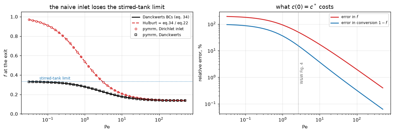
pymrm Dirichlet-inlet solve vs the Hulburt closed form: worst 9.37e-07 over Pe = 0.0316 to 501, n = 1200

       Pe    f true   f naive   err in f   X true  X naive   err in X
    0.100    0.3262    0.9104     179.1 %   0.6738   0.0896     -86.7 %
    0.500    0.3021    0.6842     126.5 %   0.6979   0.3158     -54.7 %
    1.000    0.2794    0.5384      92.7 %   0.7206   0.4616     -35.9 %
    2.667    0.2344    0.3509      49.7 %   0.7656   0.6491     -15.2 %
   10.000    0.1773    0.2076      17.1 %   0.8227   0.7924      -3.7 %
   50.000    0.1456    0.1512       3.9 %   0.8544   0.8488      -0.7 %
  200.000    0.1380    0.1394       1.0 %   0.8620   0.8606      -0.2 %

As Pe -> 0 the naive inlet gives f -> 1.0000, i.e. NO conversion,
where the stirred-tank answer is 1/(1+R).
That is Wehner & Wilhelm's objection, as a number.
What check 5 cannot see. It compares two boundary conditions inside one model; it says nothing about whether the axial-dispersion model itself describes a real bed. And the error it reports shrinks with \(\mathrm{Pe}\), so on a long, weakly dispersed reactor the naive inlet is nearly harmless: the last row of the table is the honest counterweight to the first.
Claims: what each number is, and how it is checked
Every number the page stands behind is registered once, in the cell below, with how it is checked (docs/claims-design.md in the gallery repository):
- a value is a result whose size is set by physics, by the closed forms or by a discretisation. CI holds it to a relative tolerance of the committed baseline, 5 % unless the cell says otherwise;
- a bound is a quantity whose size is not physics: a round-off gap between two readings of one formula or two solvers of one set of equations, an identity, a convergence order. It is checked against its stated limits on every run, on every machine, and states its basis;
- structural would mark an identity no break row can move; every identity on this page has a row that breaks it, so none is labelled structural.
The roles are decided by what each quantity is, never by its size.
def value(name, x, rtol=0.05, **kw):
    claims.value(name, x, rtol=rtol, **kw)


def bound(name, x, *, max=None, min=None, basis, note=None, structural=False):
    claims.bound(name, x, max=max, min=min, basis=basis, note=note, structural=structural)


ONE_FORMULA = "algebraically one formula; two floating-point arrangements of it"
# --- the transcriptions --------------------------------------------------------
bound("transcription_D33_vs_W20", TG["D33_vs_W20"], max=1e-14, basis="identity", note=ONE_FORMULA)
bound("transcription_D33_vs_D34", TG["D33_vs_D34"], max=1e-14, basis="identity", note=ONE_FORMULA)
bound("transcription_W21_vs_D34", TG["W21_vs_D34"], max=1e-14, basis="identity", note=ONE_FORMULA)
bound("transcription_D33_vs_W22", TG["D33_vs_W22"], max=1e-14, basis="identity", note=ONE_FORMULA)
value("transcription_one_digit_misread", MISREAD_ONE,
      note="eq. 33's second numerator coefficient read as 1 instead of 2")
# --- check 1: the closed vessel against eq. 34 ---------------------------------
value("closed_form_rel_err_n800", REF_DEV, note="outlet face, van Leer, n = 800")
value("closed_form_rel_err_n1600", ERR_TV, note="outlet face, van Leer, n = 1600")
value("closed_form_rel_err_n1600_last_cell", ERR_TV_CELL,
      note="the same solve read at the last cell centre (pitfall P8)")
bound("observed_order_vanleer", LAD["order_tv"], min=1.8, max=2.2, basis="theory",
      note="van Leer TVD on a smooth profile is second order; face read, n 800 to 1600")
bound("observed_order_vanleer_last_cell", LAD["order_cell"], min=1.8, max=2.2, basis="theory",
      note="dc/dz = 0 at the outlet, so the half-cell offset is second order too")
bound("observed_order_upwind", LAD["order_up"], min=0.9, max=1.1, basis="theory",
      note="first-order upwind")
bound("closed_newton_vs_deferred", GAP_CLOSED, max=1e-13, basis="tolerance",
      note="the same TVD equations by Newton with the correction-form residual "
           "(step 1e-12) and deferred correction (sweep change 1e-14); exit values over "
           "the ladder")
bound("closed_newton_full_residual_vs_deferred", GAP_CLOSED_FULL, max=1e-10, basis="tolerance",
      note="Newton with the residual written in full stops at its round-off floor, "
           "which depends on the BLAS kernel; n = 800 and 1600")
bound("closed_exit_factorisation_spread", FACT_SPREAD, max=5e-13, basis="tolerance",
      note="exit with the upwind operator factorised under permc_spec MMD_ATA against the "
           "default ordering, n = 800 and 1600")
value("closed_last_cell_over_face_n1600", CELL_OVER_FACE,
      note="last-cell error over face error against eq. 34, n = 1600")
value("closed_outlet_face_vs_last_cell", OUTLET_FACE_GAP,
      note="closed vessel n = 800: outlet face value against c_N, relative")
value("conversion_at_ww_fig4", CONVERSION, rtol=1e-5, note="1 - f(exit) at n = 800")
value("closed_vessel_inlet_step", INLET_STEP, note="1 - f(0+) from eq. 22")
value("upwind_pe_eff_residual_n1600", PE_EFF_RES[-1])
bound("upwind_pe_eff_residual_order", PE_EFF_ORDER, min=1.8, max=2.2, basis="theory",
      note="numerical diffusivity u dz/2 is the leading upwind error, so the rest is O(dz^2)")
value("upwind_pe_eff_at_pe200_n200", PE_EFF_200, rtol=1e-6, note="1/(1/Pe + dz/2), closed form")
# --- check 2: the Peclet sweep and the limits -----------------------------------
value("pe_sweep_worst_rel_err", SWEEP_WORST, note="outlet face, n = 1600")
value("pe_sweep_worst_last_cell", SWEEP_WORST_CELL, note="last cell centre, n = 1600")
value("pe_sweep_rel_err_at_pe1e4", SWEEP_FACE[I_1E4], note="outlet face")
value("pe_sweep_last_cell_at_pe1e4", SWEEP_CELL[I_1E4], note="last cell centre")
value("plug_flow_limit_eq35", LIM["plug"], note="eq. 34 at Pe = 1e8 against eq. 35")
value("stirred_tank_limit_eq36", LIM["cstr"], note="eq. 34 at Pe = 1e-8 against eq. 36")
bound("eq37_residual_order_in_inv_pe", LIM["order"], min=1.9, max=2.1, basis="theory",
      note="eq. 37 is the first-order term of an expansion in 1/Pe")
value("eq37_residual_order_full_range", LIM["order_all"],
      note="fit including the pre-asymptotic end Pe < 1e3")
value("eq37_rel_err_pe100", LIM["dev100"])
# --- check 3: three sections -----------------------------------------------------
value("three_section_vs_eq33", TS_DEV)
value("three_section_exit_spread", TS_SPREAD,
      note="spread over Pe_a and Pe_c of f(exit) against eq. 21; end-section truncation "
           "and grid")
bound("three_section_newton_vs_deferred", TS_GAP, max=1e-9, basis="tolerance",
      note="the same TVD equations by Newton (step 1e-12) and deferred correction "
           "(sweep change 1e-11) on the stretched grids; largest cell difference")
value("three_section_fore_vs_eq19", TP["fore"])
value("three_section_bed_vs_eq20", TP["bed"])
value("three_section_exit_vs_eq21", TP["exit"])
bound("three_section_fore_flux_truncation", TP["flux"], max=1e-8, basis="chosen",
      note="upstream section 20 decay lengths: the truncation estimate (1 - f(0)) exp(-20) "
           "is 6.8e-10, and the round-off floor of the long uniform grid is of that size")
value("three_section_fore_flux_estimate", TP["flux_est"], note="(1 - f(0)) exp(-P), closed form")
bound("three_section_after_flat", TP["flat"], max=1e-9, basis="identity",
      note="no source and constant D downstream force c_i = c_(i+1) for any Pe_c")
bound("after_truncation_flat", TRUNC_FLAT, max=1e-9, basis="identity",
      note="after section cut to 2 and 0.2 decay lengths; same identity")
bound("after_truncation_bed_change", TRUNC_BED, max=1e-9, basis="identity",
      note="the bed is independent of the after-section length")
bound("face_average_order_arithmetic", FL["order_a"], min=0.9, max=1.1, basis="theory",
      note="an O(1) flux error at the jump face gives a first-order error")
bound("face_average_order_harmonic", FL["order_h"], min=1.8, max=2.2, basis="theory",
      note="the harmonic mean is the series resistance of the two half cells")
value("face_average_arith_fore_n400", FL["a"][I400])
for i, n_b in enumerate(N_BED):
    value(f"face_average_ratio_n{n_b}", FL["ratio"][i])
value("face_average_first_bed_cell_harmonic", SF["harmonic"][0], rtol=1e-6)
value("face_average_first_bed_cell_shift", SF["first_shift"])
value("face_average_exit_shift", SF["exit_shift"], rtol=0.1,
      note="the arithmetic mean moves f(exit) by this; a difference of two solves, each "
           "at a residual floor about 1e-12")
value("face_average_arith_bed_vs_eq33", SF["arithmetic"][2])
value("three_section_grad_at_exit_n800", abs(GS["solve"][-1]))
value("grad_at_exit_fit_bias_on_exact_n800", abs(GS["bias"][-1]))
value("grad_at_exit_residual_n800", abs(GS["resid"][-1]))
value("grad_at_exit_estimator_share", GS["share"])
bound("grad_at_exit_residual_order", GS["order"], min=1.8, max=2.2, basis="theory",
      note="the solve's own second-order error seen through the same fit")
bound("grad_at_exit_last_bed_vs_after_gap", GS["gap"], max=1e-13, basis="identity",
      note="flat after section: last bed cell equals first after cell")
value("inlet_cell_step_pe_a_1", abs(JUMPS[1]))
value("inlet_cell_step_pe_a_1000", abs(JUMPS[-1]))
value("inlet_step_ratio_pe_a_1", STEP_RATIO)
value("inlet_first_bed_cell_spread", F0_SPREAD, note="over Pe_a = 0.3 to 1000, n_b = 200")
# --- check 4: defects ------------------------------------------------------------
value("defect_inlet_sign_flip", BREAK_TAB["inlet BC: sign of a flipped (outward normal)"])
value("defect_naive_dirichlet_inlet", BREAK_TAB["inlet BC: naive Dirichlet c(0) = c*"])
value("defect_inlet_a_one", BREAK_TAB["inlet BC: a = D but D taken as 1, not 1/Pe"])
value("defect_outlet_sign_flip", BREAK_TAB["outlet BC: sign of a flipped"],
      note="equal to the model's own deviation: the outlet sign is absent from the system")
bound("defect_outlet_dirichlet", BREAK_TAB["outlet BC: Dirichlet c(L) = 0"], min=0.5,
      basis="chosen", note="the defect drives f(exit) to zero; the claim is that the check sees it")
bound("defect_wrong_nu", BREAK_TAB["construct_div nu = 1 (cylindrical, wrong)"], min=0.5,
      basis="chosen", note="the defect drives f(exit) to zero; the claim is that the check sees it")
value("defect_reaction_sign", BREAK_TAB["reaction term sign flipped"])
value("defect_coarse_n10", BREAK_TAB["grid coarsened to n = 10"])
value("defect_upwind_n800", BREAK_TAB["upwind only, no TVD"])
value("undergrid_pe200_vanleer", UNDERGRID["van Leer"])
value("undergrid_pe200_upwind", UNDERGRID["upwind"])
bound("outlet_sign_system_change", OUTLET_CHANGE, max=0.0, basis="identity",
      note="b = d = 0 at the outlet: a multiplies nothing in the assembled system")
value("inlet_sign_system_change", INLET_CHANGE[0])
value("outlet_flux_exit_a_plus", OUT_D[1.0], rtol=1e-3)
value("outlet_flux_exit_a_minus", OUT_D[-1.0], rtol=1e-3)
# --- check 5: the naive inlet ------------------------------------------------------
value("dirichlet_vs_hulburt_closed_form", HULBURT_DEV, note="outlet face, n = 1200")
value("dirichlet_inlet_error_at_ww_fig4", naive_error(PE_B)[0], note="closed form")
value("naive_f_error_pe0p1", naive_error(0.1)[0], note="closed form")
value("naive_f_error_pe200", naive_error(200.0)[0], note="closed form")
value("naive_conversion_error_at_ww_fig4", abs(naive_error(PE_B)[1]), note="closed form")
value("naive_f_limit_pe_to_zero", NAIVE_LIMIT, rtol=1e-4, note="at Pe = 1e-6")
print(f"{len(claims.metrics)} claims: "
      + ", ".join(f"{sum(c['kind'] == k for c in claims.metrics.values())} {k}"
                  for k in ("value", "bound", "exact")))
83 claims: 59 value, 24 bound, 0 exactThe defect-injection table
Each row breaks one thing on purpose, re-runs the computation behind one or more claims with the defect in place (a changed argument of the same function, never a typed number), and hands the result to claims.breaks, which records whether the claim’s own check (its tolerance or its bound) catches it. Every claim that is not structural must be failed by at least one row, and the last cell of the page raises otherwise.
BREAK = []


def brk(name, metric, broken):
    """One injected defect: ``broken`` is what claim ``metric`` becomes with it."""
    caught = claims.breaks(name, metric, broken)
    BREAK.append((name, metric, claims[metric], float(broken), caught))


# the transcriptions: a mis-read coefficient in each reading
TG_33 = transcription_gaps(num_coeff=(2.0, 1.0))
brk("eq. 33 numerator 2(1-a) read as 1(1-a)", "transcription_D33_vs_W20", TG_33["D33_vs_W20"])
brk("eq. 33 numerator 2(1-a) read as 1(1-a)", "transcription_D33_vs_D34", TG_33["D33_vs_D34"])
brk("eq. 33 numerator 2(1-a) read as 1(1-a)", "transcription_D33_vs_W22", TG_33["D33_vs_W22"])
brk("eq. 21 leading 2 read as 1", "transcription_W21_vs_D34",
    transcription_gaps(w21_lead=1.0)["W21_vs_D34"])
brk("Fig. 4 label Pe_b read as 2.0", "transcription_one_digit_misread",
    transcription_gaps(Pe=2.0, num_coeff=(2.0, 1.0))["D33_vs_W20"])
# check 1
LAD_UP = closed_ladder(ns=(800, 1600), limiter=None)
brk("upwind instead of van Leer", "closed_form_rel_err_n1600", LAD_UP["tv_face"][-1])
brk("upwind instead of van Leer", "closed_last_cell_over_face_n1600",
    LAD_UP["tv_cell"][-1] / LAD_UP["tv_face"][-1])
brk("Newton residual written in full, other ordering", "closed_exit_factorisation_spread",
    factorisation_spread(residual="full"))
brk("closed vessel on 400 cells", "closed_outlet_face_vs_last_cell",
    outlet_face_vs_last_cell(n=400)[0])
brk("upwind instead of van Leer", "closed_form_rel_err_n1600_last_cell", LAD_UP["tv_cell"][-1])
brk("upwind instead of van Leer", "observed_order_vanleer", LAD_UP["order_tv"])
brk("upwind instead of van Leer", "observed_order_vanleer_last_cell", LAD_UP["order_cell"])
brk("naive Dirichlet inlet", "observed_order_upwind",
    closed_ladder(ns=(800, 1600), inlet="dirichlet", limiter=None)["order_up"])
brk("deferred-correction route given minmod", "closed_newton_vs_deferred",
    float(np.max(closed_ladder(ns=(800, 1600), second_limiter=minmod)["gap"])))
brk("Newton residual written in full", "closed_newton_vs_deferred", GAP_CLOSED_FULL)
brk("deferred-correction route given minmod", "closed_newton_full_residual_vs_deferred",
    float(np.max(closed_ladder(ns=(800, 1600), second_limiter=minmod,
                               residual="full")["gap"])))
_up800 = ClosedVessel(PE_B, R_REF, n=800).solve(limiter=None)
brk("upwind instead of van Leer", "conversion_at_ww_fig4", 1 - _up800.c_exit)
brk("upwind instead of van Leer", "closed_form_rel_err_n800",
    abs(_up800.c_exit / F_EX - 1))
brk("eq. 22 exponents a Pe/2 read as Pe/2", "closed_vessel_inlet_step",
    1 - f0_W22(PE_B, R_REF, a_in_exp=False))
_pe_eff_b = pe_eff_residuals(factor=1.0)
brk("numerical diffusivity taken as u dz", "upwind_pe_eff_residual_n1600", _pe_eff_b[0][-1])
brk("numerical diffusivity taken as u dz", "upwind_pe_eff_residual_order", _pe_eff_b[1])
brk("numerical diffusivity taken as u dz", "upwind_pe_eff_at_pe200_n200",
    pe_eff(200.0, 200, factor=1.0))
# check 2
_sw_up = pe_sweep(limiter=None)
brk("upwind instead of van Leer", "pe_sweep_worst_rel_err", _sw_up[1].max())
brk("upwind instead of van Leer", "pe_sweep_rel_err_at_pe1e4", _sw_up[1][I_1E4])
_sw_800 = pe_sweep(n=800)
brk("sweep on 800 cells", "pe_sweep_worst_last_cell", _sw_800[2].max())
brk("sweep on 800 cells", "pe_sweep_last_cell_at_pe1e4", _sw_800[2][I_1E4])
_lim_lead = limit_checks(lead=2.0)
brk("eq. 34 numerator 4a read as 2a", "plug_flow_limit_eq35", _lim_lead["plug"])
brk("eq. 34 numerator 4a read as 2a", "stirred_tank_limit_eq36", _lim_lead["cstr"])
_lim_pow = limit_checks(power=1.0)
brk("eq. 37 correction R^2/Pe read as R/Pe", "eq37_residual_order_in_inv_pe", _lim_pow["order"])
brk("eq. 37 correction R^2/Pe read as R/Pe", "eq37_residual_order_full_range",
    _lim_pow["order_all"])
brk("eq. 37 correction R^2/Pe read as R/Pe", "eq37_rel_err_pe100", _lim_pow["dev100"])
# check 3
_ts_200 = ts_sweep(n_b=200)
brk("bed on 200 cells", "three_section_vs_eq33", _ts_200[:, 0].max())
brk("end sections cut to 3 decay lengths", "three_section_exit_spread",
    np.ptp(ts_sweep(P=3.0)[:, 1]))
brk("deferred correction stopped at a sweep change of 1e-6", "three_section_newton_vs_deferred",
    ts_sweep(deferred_tol=1e-6)[:, 2].max())
_tp_up = ts_profile(limiter=None)
brk("three sections solved upwind", "three_section_fore_vs_eq19", _tp_up["fore"])
brk("three sections solved upwind", "three_section_bed_vs_eq20", _tp_up["bed"])
brk("three sections solved upwind", "three_section_exit_vs_eq21", _tp_up["exit"])
brk("upstream section cut to 10 decay lengths", "three_section_fore_flux_truncation",
    ts_profile(P=10.0)["flux"])
brk("eq. 22 exponents a Pe/2 read as Pe/2", "three_section_fore_flux_estimate",
    ts_profile(a_in_exp=False)["flux_est"])
_fl_hh = face_ladder(pair=("harmonic", "harmonic"))
_fl_aa = face_ladder(pair=("arithmetic", "arithmetic"))
brk("harmonic mean in both runs", "face_average_order_arithmetic", _fl_hh["order_a"])
brk("arithmetic mean in both runs", "face_average_order_harmonic", _fl_aa["order_h"])
brk("harmonic mean in both runs", "face_average_arith_fore_n400", _fl_hh["a"][I400])
for i, n_b in enumerate(N_BED):
    brk("harmonic mean in both runs", f"face_average_ratio_n{n_b}", _fl_hh["ratio"][i])
_sf_100 = silent_failure(n_b=100)
brk("bed on 100 cells", "face_average_first_bed_cell_harmonic", _sf_100["harmonic"][0])
brk("bed on 100 cells", "face_average_first_bed_cell_shift", _sf_100["first_shift"])
brk("bed on 100 cells", "face_average_exit_shift", _sf_100["exit_shift"])
brk("bed on 100 cells", "face_average_arith_bed_vs_eq33", _sf_100["arithmetic"][2])
_gs_half = grad_study(n_bs=(100, 200, 400))
brk("finest bed 400 cells, not 800", "three_section_grad_at_exit_n800", abs(_gs_half["solve"][-1]))
brk("finest bed 400 cells, not 800", "grad_at_exit_fit_bias_on_exact_n800",
    abs(_gs_half["bias"][-1]))
brk("finest bed 400 cells, not 800", "grad_at_exit_residual_n800", abs(_gs_half["resid"][-1]))
_gs_up = grad_study(limiter=None)
brk("three sections solved upwind", "grad_at_exit_estimator_share", _gs_up["share"])
brk("fit window one cell downstream, across z = 1", "grad_at_exit_residual_order",
    grad_study(shift=1)["order"])
_steps_100 = inlet_steps(n_b=100)
brk("bed on 100 cells", "inlet_cell_step_pe_a_1", abs(_steps_100[0][1]))
brk("bed on 100 cells", "inlet_cell_step_pe_a_1000", abs(_steps_100[0][-1]))
brk("bed on 100 cells", "inlet_step_ratio_pe_a_1", INLET_STEP / _steps_100[0][1])
brk("bed on 100 cells", "inlet_first_bed_cell_spread", _steps_100[1])
# the identities of the three-section problem fail once the reaction leaks downstream
_tp_leak = ts_profile(react_past_bed=True)
brk("reaction runs on past z = 1", "three_section_after_flat", _tp_leak["flat"])
_tr_leak = truncation_study(react_past_bed=True)
brk("reaction runs on past z = 1", "after_truncation_flat", _tr_leak[0])
brk("reaction runs on past z = 1", "after_truncation_bed_change", _tr_leak[1])
brk("reaction runs on past z = 1", "grad_at_exit_last_bed_vs_after_gap",
    grad_study(n_bs=(100, 200), react_past_bed=True)["gap"])
brk("outlet d = 0.05 with a flipped", "outlet_sign_system_change",
    max(system_change(base=dict(outlet_d=0.05), outlet_a=-1.0, outlet_d=0.05)))
# check 4: the defect itself changed, then a mis-read reference
for label, kw in DEFECTS:
    name = {"inlet BC: sign of a flipped (outward normal)": "defect_inlet_sign_flip",
            "inlet BC: naive Dirichlet c(0) = c*": "defect_naive_dirichlet_inlet",
            "inlet BC: a = D but D taken as 1, not 1/Pe": "defect_inlet_a_one",
            "outlet BC: sign of a flipped": "defect_outlet_sign_flip",
            "reaction term sign flipped": "defect_reaction_sign",
            "grid coarsened to n = 10": "defect_coarse_n10",
            "upwind only, no TVD": "defect_upwind_n800"}.get(label)
    if name:
        brk("eq. 34 numerator 4a read as 2a", name, defect_deviation(kw, lead=2.0)[1])
brk("defect undone: outlet c(L) = 0 replaced by dc/dz = 0", "defect_outlet_dirichlet",
    defect_deviation({})[1])
brk("defect undone: nu = 0", "defect_wrong_nu", defect_deviation(dict(nu=0))[1])
for row, name, kw in [
        ("inlet a = -D/(2u) instead of -D/u", "defect_inlet_sign_flip",
         dict(inlet_a=-0.5 * D_REF)),
        ("naive Dirichlet inlet with d = 0.9", "defect_naive_dirichlet_inlet",
         dict(inlet="dirichlet", inlet_d=0.9)),
        ("inlet a = 2 instead of 1", "defect_inlet_a_one", dict(inlet_a=2.0)),
        ("outlet a flipped with d = 0.05", "defect_outlet_sign_flip",
         dict(outlet_a=-1.0, outlet_d=0.05)),
        ("reaction sign flipped at half strength", "defect_reaction_sign", dict(r_sign=-0.5)),
        ("grid coarsened to n = 20", "defect_coarse_n10", dict(n=20)),
        ("upwind on 400 cells", "defect_upwind_n800", dict(limiter=None, n=400))]:
    brk(row, name, defect_deviation(kw)[1])
brk("eq. 34 numerator 4a read as 2a", "undergrid_pe200_vanleer",
    defect_deviation(dict(n=10), Pe=200.0, lead=2.0)[1])
brk("eq. 34 numerator 4a read as 2a", "undergrid_pe200_upwind",
    defect_deviation(dict(n=10, limiter=None), Pe=200.0, lead=2.0)[1])
brk("inlet sign not flipped", "inlet_sign_system_change", system_change(inlet_a=D_REF)[0])
_out_d0 = outlet_flux_exits(d_out=0.0)
brk("outlet d = 0", "outlet_flux_exit_a_plus", _out_d0[1.0])
brk("outlet d = 0", "outlet_flux_exit_a_minus", _out_d0[-1.0])
# check 5
brk("bed on 600 cells", "dirichlet_vs_hulburt_closed_form", hulburt_check(n=600)[2])
brk("eq. 22 exponents a Pe/2 read as Pe/2", "dirichlet_inlet_error_at_ww_fig4",
    naive_error(PE_B, False)[0])
brk("eq. 22 exponents a Pe/2 read as Pe/2", "naive_f_error_pe0p1", naive_error(0.1, False)[0])
brk("eq. 22 exponents a Pe/2 read as Pe/2", "naive_f_error_pe200", naive_error(200.0, False)[0])
brk("eq. 22 exponents a Pe/2 read as Pe/2", "naive_conversion_error_at_ww_fig4",
    abs(naive_error(PE_B, False)[1]))
brk("Hulburt's division by f(0) dropped", "naive_f_limit_pe_to_zero",
    naive_error(1e-6, normalise=False)[3])

print(f"{'injected defect':<54} {'claim':<38} {'clean':>16} {'broken':>16}  caught")
for name, metric, clean, broken, caught in BREAK:
    # a bound's own value is round-off or a tolerance effect: shown as this run's
    is_bound = claims.metrics[metric]["kind"] == "bound"
    shown = f"(here {clean:.1e})" if is_bound else f"{clean:10.3g}"
    broke = f"(here {broken:.1e})" if is_bound else f"{broken:10.3g}"
    print(f"{name[:54]:<54} {metric[:38]:<38} {shown:>16} {broke:>16}  "
          f"{'yes' if caught else 'NO'}")
_caught = {m for _, m, _, _, c in BREAK if c}
_structural = sorted(k for k, c in claims.metrics.items() if c.get("structural"))
_open = sorted(k for k in claims.metrics if k not in _caught and k not in _structural)
print(f"\n{len(BREAK)} rows; {len(_caught)} of {len(claims.metrics)} claims are failed by at "
      f"least one row; structural: {', '.join(_structural) or 'none'}; "
      f"open: {', '.join(_open) or 'none'}")
_uncaught = [(n, m) for n, m, _, _, c in BREAK if not c]
print("rows that do not fail their claim: " + (", ".join(f"{n} -> {m}" for n, m in _uncaught)
                                               or "none"))
injected defect claim clean broken caught
eq. 33 numerator 2(1-a) read as 1(1-a) transcription_D33_vs_W20 (here 1.1e-16) (here 2.9e-02) yes
eq. 33 numerator 2(1-a) read as 1(1-a) transcription_D33_vs_D34 (here 8.3e-17) (here 2.9e-02) yes
eq. 33 numerator 2(1-a) read as 1(1-a) transcription_D33_vs_W22 (here 0.0e+00) (here 5.4e-04) yes
eq. 21 leading 2 read as 1 transcription_W21_vs_D34 (here 5.6e-17) (here 1.2e-01) yes
Fig. 4 label Pe_b read as 2.0 transcription_one_digit_misread 0.0293 0.0343 yes
upwind instead of van Leer closed_form_rel_err_n1600 3.85e-08 0.000176 yes
upwind instead of van Leer closed_last_cell_over_face_n1600 5.75 1 yes
Newton residual written in full, other ordering closed_exit_factorisation_spread (here 1.9e-13) (here 1.5e-12) yes
closed vessel on 400 cells closed_outlet_face_vs_last_cell 1.04e-06 4.15e-06 yes
upwind instead of van Leer closed_form_rel_err_n1600_last_cell 2.22e-07 0.000176 yes
upwind instead of van Leer observed_order_vanleer (here 2.0e+00) (here 1.0e+00) yes
upwind instead of van Leer observed_order_vanleer_last_cell (here 2.0e+00) (here 1.0e+00) yes
naive Dirichlet inlet observed_order_upwind (here 1.0e+00) (here 1.6e-03) yes
deferred-correction route given minmod closed_newton_vs_deferred (here 6.7e-16) (here 1.5e-07) yes
Newton residual written in full closed_newton_vs_deferred (here 6.7e-16) (here 1.2e-12) yes
deferred-correction route given minmod closed_newton_full_residual_vs_deferre (here 1.2e-12) (here 1.5e-07) yes
upwind instead of van Leer conversion_at_ww_fig4 0.766 0.765 yes
upwind instead of van Leer closed_form_rel_err_n800 1.51e-07 0.000351 yes
eq. 22 exponents a Pe/2 read as Pe/2 closed_vessel_inlet_step 0.332 0.82 yes
numerical diffusivity taken as u dz upwind_pe_eff_residual_n1600 1.18e-07 0.000175 yes
numerical diffusivity taken as u dz upwind_pe_eff_residual_order (here 2.0e+00) (here 1.0e+00) yes
numerical diffusivity taken as u dz upwind_pe_eff_at_pe200_n200 133 100 yes
upwind instead of van Leer pe_sweep_worst_rel_err 3.62e-07 0.00125 yes
upwind instead of van Leer pe_sweep_rel_err_at_pe1e4 6.18e-08 0.00125 yes
sweep on 800 cells pe_sweep_worst_last_cell 0.000188 0.000404 yes
sweep on 800 cells pe_sweep_last_cell_at_pe1e4 0.000188 0.000404 yes
eq. 34 numerator 4a read as 2a plug_flow_limit_eq35 4.55e-08 0.5 yes
eq. 34 numerator 4a read as 2a stirred_tank_limit_eq36 2.22e-09 0.5 yes
eq. 37 correction R^2/Pe read as R/Pe eq37_residual_order_in_inv_pe (here 2.0e+00) (here 1.0e+00) yes
eq. 37 correction R^2/Pe read as R/Pe eq37_residual_order_full_range 1.95 0.931 yes
eq. 37 correction R^2/Pe read as R/Pe eq37_rel_err_pe100 0.00112 0.0181 yes
bed on 200 cells three_section_vs_eq33 7.83e-06 3.1e-05 yes
end sections cut to 3 decay lengths three_section_exit_spread 4.96e-08 0.000151 yes
deferred correction stopped at a sweep change of 1e-6 three_section_newton_vs_deferred (here 1.2e-11) (here 3.6e-07) yes
three sections solved upwind three_section_fore_vs_eq19 9.03e-07 0.000534 yes
three sections solved upwind three_section_bed_vs_eq20 8.48e-07 0.000536 yes
three sections solved upwind three_section_exit_vs_eq21 8.08e-07 0.000704 yes
upstream section cut to 10 decay lengths three_section_fore_flux_truncation (here 1.2e-09) (here 1.5e-05) yes
eq. 22 exponents a Pe/2 read as Pe/2 three_section_fore_flux_estimate 6.84e-10 1.69e-09 yes
harmonic mean in both runs face_average_order_arithmetic (here 1.0e+00) (here 2.0e+00) yes
arithmetic mean in both runs face_average_order_harmonic (here 2.0e+00) (here 1.0e+00) yes
harmonic mean in both runs face_average_arith_fore_n400 0.000313 9.03e-07 yes
harmonic mean in both runs face_average_ratio_n100 84.4 1 yes
harmonic mean in both runs face_average_ratio_n200 172 1 yes
harmonic mean in both runs face_average_ratio_n400 347 1 yes
harmonic mean in both runs face_average_ratio_n800 697 1 yes
bed on 100 cells face_average_first_bed_cell_harmonic 0.667 0.664 yes
bed on 100 cells face_average_first_bed_cell_shift 7.93e-07 1.22e-05 yes
bed on 100 cells face_average_exit_shift 9.33e-10 5.82e-08 yes
bed on 100 cells face_average_arith_bed_vs_eq33 1.64e-06 2.51e-05 yes
finest bed 400 cells, not 800 three_section_grad_at_exit_n800 5.88e-06 2.34e-05 yes
finest bed 400 cells, not 800 grad_at_exit_fit_bias_on_exact_n800 4.96e-06 1.97e-05 yes
finest bed 400 cells, not 800 grad_at_exit_residual_n800 9.15e-07 3.67e-06 yes
three sections solved upwind grad_at_exit_estimator_share 0.844 0.961 yes
fit window one cell downstream, across z = 1 grad_at_exit_residual_order (here 2.0e+00) (here -9.1e-01) yes
bed on 100 cells inlet_cell_step_pe_a_1 0.00296 0.00596 yes
bed on 100 cells inlet_cell_step_pe_a_1000 0.266 0.302 yes
bed on 100 cells inlet_step_ratio_pe_a_1 112 55.7 yes
bed on 100 cells inlet_first_bed_cell_spread 3.73e-05 0.000121 yes
reaction runs on past z = 1 three_section_after_flat (here 8.2e-11) (here 1.4e-01) yes
reaction runs on past z = 1 after_truncation_flat (here 1.7e-12) (here 1.1e-01) yes
reaction runs on past z = 1 after_truncation_bed_change (here 3.2e-13) (here 4.9e-02) yes
reaction runs on past z = 1 grad_at_exit_last_bed_vs_after_gap (here 5.3e-16) (here 2.5e-03) yes
outlet d = 0.05 with a flipped outlet_sign_system_change (here 0.0e+00) (here 3.0e+01) yes
eq. 34 numerator 4a read as 2a defect_inlet_sign_flip 1.97 4.95 yes
eq. 34 numerator 4a read as 2a defect_naive_dirichlet_inlet 0.497 1.99 yes
eq. 34 numerator 4a read as 2a defect_inlet_a_one 0.356 0.288 yes
eq. 34 numerator 4a read as 2a defect_outlet_sign_flip 1.51e-07 1 yes
eq. 34 numerator 4a read as 2a defect_reaction_sign 26.1 51.1 yes
eq. 34 numerator 4a read as 2a defect_coarse_n10 6.29e-05 1 yes
eq. 34 numerator 4a read as 2a defect_upwind_n800 0.000351 1 yes
defect undone: outlet c(L) = 0 replaced by dc/dz = 0 defect_outlet_dirichlet (here 1.0e+00) (here 1.5e-07) yes
defect undone: nu = 0 defect_wrong_nu (here 1.0e+00) (here 1.5e-07) yes
inlet a = -D/(2u) instead of -D/u defect_inlet_sign_flip 1.97 0.991 yes
naive Dirichlet inlet with d = 0.9 defect_naive_dirichlet_inlet 0.497 0.347 yes
inlet a = 2 instead of 1 defect_inlet_a_one 0.356 0.59 yes
outlet a flipped with d = 0.05 defect_outlet_sign_flip 1.51e-07 0.0534 yes
reaction sign flipped at half strength defect_reaction_sign 26.1 17.5 yes
grid coarsened to n = 20 defect_coarse_n10 6.29e-05 7.62e-05 yes
upwind on 400 cells defect_upwind_n800 0.000351 0.000703 yes
eq. 34 numerator 4a read as 2a undergrid_pe200_vanleer 0.00319 1.01 yes
eq. 34 numerator 4a read as 2a undergrid_pe200_upwind 0.18 1.36 yes
inlet sign not flipped inlet_sign_system_change 1.8e+03 0 yes
outlet d = 0 outlet_flux_exit_a_plus 0.247 0.234 yes
outlet d = 0 outlet_flux_exit_a_minus 0.222 0.234 yes
bed on 600 cells dirichlet_vs_hulburt_closed_form 9.37e-07 3.47e-06 yes
eq. 22 exponents a Pe/2 read as Pe/2 dirichlet_inlet_error_at_ww_fig4 0.497 4.56 yes
eq. 22 exponents a Pe/2 read as Pe/2 naive_f_error_pe0p1 1.79 2.2 yes
eq. 22 exponents a Pe/2 read as Pe/2 naive_f_error_pe200 0.0099 6.32 yes
eq. 22 exponents a Pe/2 read as Pe/2 naive_conversion_error_at_ww_fig4 0.152 1.4 yes
Hulburt's division by f(0) dropped naive_f_limit_pe_to_zero 1 0.333 yes
91 rows; 83 of 83 claims are failed by at least one row; structural: none; open: none
rows that do not fail their claim: noneWhat pymrm adds
To the result: nothing. Danckwerts’ conditions are right, Wehner & Wilhelm’s derivation is correct, and the closed form is exact. This page reproduces them; it does not improve them.
What the page measures that neither paper states, using pymrm as the solver (the measurements are the page’s, not features of the library):
- The naive inlet’s error, as a function of Peclet number. Wehner & Wilhelm say Hulburt’s solution “is not consistent with the limit of a stirred reactor”. Check 5 turns that into a curve, from a large error in \(f\) at \(\mathrm{Pe} = 0.1\) to a small one by \(\mathrm{Pe} = 200\), and complete loss of conversion as \(\mathrm{Pe}\to0\). Both papers had the algebra; neither plotted it.
- The outward-normal trap is asymmetric, and the safe-looking end is the dangerous one. At the inlet a flipped sign is a large error. At the outlet it is undetectable by any test whatsoever: with \(b = d = 0\) the assembled matrix and right-hand side are bit-identical for \(a = +1\), \(a = -1\) and \(a = 10^{7}\), so there is no difference to detect rather than a small one. Make \(d\) non-zero and the sign matters again. Proving your outlet condition works proves nothing about your inlet condition.
- What the discretisation does to a boundary-condition study. Bare upwind convection adds a numerical diffusivity \(u\,\Delta z/2\), which is indistinguishable from lowering the Peclet number, and check 1 shows it is that, to second order. A study of inlet conditions at high Peclet number done on an upwind grid can therefore measure its own truncation error and call it physics. And where the outlet value is read matters as much: at high \(\mathrm{Pe}\) the outlet layer is thinner than a cell, and the last cell value lies far from the exit the scheme computes.
What the library provides here. The {"a", "b", "d"} boundary dictionaries and describe_bc, which prints the equation each one imposes; ConvFluxTVD, whose exact Jacobian lets newton(..., damping="monotone") solve the steady van Leer equations directly; compute_boundary_values, which reads the outlet on the face the scheme transported; and construct_coefficient_matrix for the face diffusivities of the three-section problem. The harmonic mean itself is one line of model.py, not a library feature.
What is deliberately not claimed. No experimental validation: neither paper measures anything that tests these boundary conditions, and the one experimental figure in Danckwerts (the Raschig-ring F-diagram) belongs to his open-vessel residence-time analysis, which he himself says cannot be carried into the reactor problem. Nothing on this page tests whether a real packed bed obeys the axial-dispersion model at all, only what the model means once you have adopted it. And the residence-time half of Danckwerts 1953 (the \(F\)- and \(C\)-diagrams, hold-back, segregation, the laminar-pipe distribution) is not built here; A2.4 is the catalog entry for that material.
print("The numbers behind the three points above, from the cells that computed them:")
print(f"  1. naive inlet, error in f: {100 * claims['naive_f_error_pe0p1']:.0f} % at Pe = 0.1, "
      f"{100 * claims['dirichlet_inlet_error_at_ww_fig4']:.0f} % at Pe = {PE_B}, "
      f"{100 * claims['naive_f_error_pe200']:.1f} % at Pe = 200; "
      f"f -> {claims['naive_f_limit_pe_to_zero']:.4f} as Pe -> 0")
print(f"  2. inlet sign flipped: {100 * claims['defect_inlet_sign_flip']:.0f} % in f(exit); "
      f"outlet sign flipped: system change {claims['outlet_sign_system_change']:.1f}")
print(f"  3. a 200-cell upwind grid at Pe = 200 runs at Pe_eff = "
      f"{claims['upwind_pe_eff_at_pe200_n200']:.0f}; at Pe = 1e4 the exit agrees with eq. 34 "
      f"to {claims['pe_sweep_rel_err_at_pe1e4']:.1e}, the last cell value lies "
      f"{claims['pe_sweep_last_cell_at_pe1e4']:.1e} from it")
The numbers behind the three points above, from the cells that computed them:
1. naive inlet, error in f: 179 % at Pe = 0.1, 50 % at Pe = 2.667, 1.0 % at Pe = 200; f -> 1.0000 as Pe -> 0
2. inlet sign flipped: 197 % in f(exit); outlet sign flipped: system change 0.0
3. a 200-cell upwind grid at Pe = 200 runs at Pe_eff = 133; at Pe = 1e4 the exit agrees with eq. 34 to 6.2e-08, the last cell value lies 1.9e-04 from itReuse
Copy ClosedVessel from model.py for any S4 model. The two bc dicts are the reusable part, and the comment above each one is the point:
D, u = 1.0 / Pe, 1.0
bc = (
    # inlet, Danckwerts eq. 31:  u c* = u c - D dc/dz  at z = 0.
    # n = -z, so dc/dn = -dc/dz  ->  (D/u) dc/dn + c = c*
    {"a": D / u, "b": 1.0, "d": c_star},
    # outlet, Danckwerts eq. 32:  dc/dz = 0 at z = L.
    # n = +z, so dc/dn = dc/dz   ->  a = 1, b = 0, d = 0
    {"a": 1.0, "b": 0.0, "d": 0.0},
)
print(describe_bc(bc, z_f))   # the equations these dicts impose, in terms of z
With several species, d becomes a vector of inlet concentrations and a becomes a vector of \(D_i/u\): one dict per boundary, broadcast over the field axis; the shape convention is (n_z, n_c), spatial axis first.
With a variable velocity (gas contraction, temperature change) discretise \(\mathrm{d}(uc)/\mathrm{d}z\) as the divergence of the flux, and set \(a = D/u\) using the inlet velocity. F2.3 records what happens when this is got wrong.
Traps this page measures.
- Read the exit with
compute_boundary_values, not from the last cell centre. At the reference Peclet number both reads converge at second order (the outlet gradient is zero), so the observed order does not reveal the difference; at high Peclet number the outlet boundary layer is thinner than a cell, the cell-centre read errs at first order (the break row “sweep on 800 cells” doubles it) and dominates the error. - At a jump in diffusivity, average \(D\) harmonically at the face. The arithmetic mean is silently wrong there (the profile stays smooth and the exit value barely moves), and what it costs is an order: first instead of second at the jump, so the penalty grows in proportion to \(n\). The page measures both rates; do not copy a single “\(N\times\) worse” figure out of it. Where the cells on the two sides of the jump differ in width, weight the harmonic mean by the half-cell distances (pitfall P2);
ThreeSectionkeeps them equal. - On a single field write the shape as
(n, 1), never(n,). It matters forNumJac(a dense Jacobian otherwise) and it is the house layout anyway. - Solve steady TVD with
ConvFluxTVDandnewton(..., damping="monotone"), and checksuccess:ClosedVessel.solveandThreeSection.solveraise when it is false. Keep the Newton step tolerance above the round-off floor of the discrete solution; checks 1 and 3 print the floors measured on this page.
Related pages. A2.3 computes the \(D\) that these conditions then close. A2.4 (tanks-in-series) is the other classical way to represent the same non-ideality; D1.2 and A2.5/A2.6 supply \(\mathrm{Pe}_{\mathrm{ax}}\) correlations for real packings.
Cite the sources, not this page:
- Danckwerts, P. V., Continuous flow systems: distribution of residence times, Chemical Engineering Science 2(1) 1-13 (1953), doi:10.1016/0009-2509(53)80001-1.
- Wehner, J. F. and Wilhelm, R. H., Boundary conditions of flow reactor, Chemical Engineering Science 6(2) 89-93 (1956), doi:10.1016/0009-2509(56)80014-6.
# Claims: prose literals checked against the computed numbers, then every
# registered number printed, agreement.json written for CI, and an exception
# raised when a claim fails its own check or has no break row.
claims.says("50 %", "dirichlet_inlet_error_at_ww_fig4")   # title cell and check 3
claims.says("179 %", "naive_f_error_pe0p1")               # title cell
claims.report();   # the semicolon keeps the notebook from echoing the payload
Claims for A2.1:
transcription_D33_vs_W20 = (here 1.1e-16) bound bound <= 1e-14 [identity]
transcription_D33_vs_D34 = (here 8.3e-17) bound bound <= 1e-14 [identity]
transcription_W21_vs_D34 = (here 5.6e-17) bound bound <= 1e-14 [identity]
transcription_D33_vs_W22 = (here 0.0e+00) bound bound <= 1e-14 [identity]
transcription_one_digit_misread = 0.029302 value rtol 0.05
closed_form_rel_err_n800 = 1.5126e-07 value rtol 0.05
closed_form_rel_err_n1600 = 3.8547e-08 value rtol 0.05
closed_form_rel_err_n1600_last_cell = 2.217e-07 value rtol 0.05
observed_order_vanleer = (here 2.0e+00) bound bound [1.8, 2.2] [theory]
observed_order_vanleer_last_cell = (here 2.0e+00) bound bound [1.8, 2.2] [theory]
observed_order_upwind = (here 1.0e+00) bound bound [0.9, 1.1] [theory]
closed_newton_vs_deferred = (here 6.7e-16) bound bound <= 1e-13 [tolerance]
closed_newton_full_residual_vs_deferred = (here 1.2e-12) bound bound <= 1e-10 [tolerance]
closed_exit_factorisation_spread = (here 1.9e-13) bound bound <= 5e-13 [tolerance]
closed_last_cell_over_face_n1600 = 5.7516 value rtol 0.05
closed_outlet_face_vs_last_cell = 1.0402e-06 value rtol 0.05
conversion_at_ww_fig4 = 0.76557 value rtol 1e-05
closed_vessel_inlet_step = 0.33188 value rtol 0.05
upwind_pe_eff_residual_n1600 = 1.1778e-07 value rtol 0.05
upwind_pe_eff_residual_order = (here 2.0e+00) bound bound [1.8, 2.2] [theory]
upwind_pe_eff_at_pe200_n200 = 133.33 value rtol 1e-06
pe_sweep_worst_rel_err = 3.6221e-07 value rtol 0.05
pe_sweep_worst_last_cell = 0.0001877 value rtol 0.05
pe_sweep_rel_err_at_pe1e4 = 6.1776e-08 value rtol 0.05
pe_sweep_last_cell_at_pe1e4 = 0.0001877 value rtol 0.05
plug_flow_limit_eq35 = 4.5462e-08 value rtol 0.05
stirred_tank_limit_eq36 = 2.2222e-09 value rtol 0.05
eq37_residual_order_in_inv_pe = (here 2.0e+00) bound bound [1.9, 2.1] [theory]
eq37_residual_order_full_range = 1.9531 value rtol 0.05
eq37_rel_err_pe100 = 0.0011157 value rtol 0.05
three_section_vs_eq33 = 7.8283e-06 value rtol 0.05
three_section_exit_spread = 4.9616e-08 value rtol 0.05
three_section_newton_vs_deferred = (here 1.2e-11) bound bound <= 1e-09 [tolerance]
three_section_fore_vs_eq19 = 9.0293e-07 value rtol 0.05
three_section_bed_vs_eq20 = 8.4843e-07 value rtol 0.05
three_section_exit_vs_eq21 = 8.0758e-07 value rtol 0.05
three_section_fore_flux_truncation = (here 1.2e-09) bound bound <= 1e-08 [chosen]
three_section_fore_flux_estimate = 6.8406e-10 value rtol 0.05
three_section_after_flat = (here 8.2e-11) bound bound <= 1e-09 [identity]
after_truncation_flat = (here 1.7e-12) bound bound <= 1e-09 [identity]
after_truncation_bed_change = (here 3.2e-13) bound bound <= 1e-09 [identity]
face_average_order_arithmetic = (here 1.0e+00) bound bound [0.9, 1.1] [theory]
face_average_order_harmonic = (here 2.0e+00) bound bound [1.8, 2.2] [theory]
face_average_arith_fore_n400 = 0.0003134 value rtol 0.05
face_average_ratio_n100 = 84.39 value rtol 0.05
face_average_ratio_n200 = 172.01 value rtol 0.05
face_average_ratio_n400 = 347.09 value rtol 0.05
face_average_ratio_n800 = 696.85 value rtol 0.05
face_average_first_bed_cell_harmonic = 0.66701 value rtol 1e-06
face_average_first_bed_cell_shift = 7.9269e-07 value rtol 0.05
face_average_exit_shift = 9.3323e-10 value rtol 0.1
face_average_arith_bed_vs_eq33 = 1.6411e-06 value rtol 0.05
three_section_grad_at_exit_n800 = 5.8782e-06 value rtol 0.05
grad_at_exit_fit_bias_on_exact_n800 = 4.9634e-06 value rtol 0.05
grad_at_exit_residual_n800 = 9.148e-07 value rtol 0.05
grad_at_exit_estimator_share = 0.84437 value rtol 0.05
grad_at_exit_residual_order = (here 2.0e+00) bound bound [1.8, 2.2] [theory]
grad_at_exit_last_bed_vs_after_gap = (here 5.3e-16) bound bound <= 1e-13 [identity]
inlet_cell_step_pe_a_1 = 0.0029639 value rtol 0.05
inlet_cell_step_pe_a_1000 = 0.26635 value rtol 0.05
inlet_step_ratio_pe_a_1 = 111.97 value rtol 0.05
inlet_first_bed_cell_spread = 3.7267e-05 value rtol 0.05
defect_inlet_sign_flip = 1.9741 value rtol 0.05
defect_naive_dirichlet_inlet = 0.49674 value rtol 0.05
defect_inlet_a_one = 0.35619 value rtol 0.05
defect_outlet_sign_flip = 1.5126e-07 value rtol 0.05
defect_outlet_dirichlet = (here 1.0e+00) bound bound >= 0.5 [chosen]
defect_wrong_nu = (here 1.0e+00) bound bound >= 0.5 [chosen]
defect_reaction_sign = 26.063 value rtol 0.05
defect_coarse_n10 = 6.2901e-05 value rtol 0.05
defect_upwind_n800 = 0.00035133 value rtol 0.05
undergrid_pe200_vanleer = 0.0031883 value rtol 0.05
undergrid_pe200_upwind = 0.18034 value rtol 0.05
outlet_sign_system_change = (here 0.0e+00) bound bound <= 0 [identity]
inlet_sign_system_change = 1802.3 value rtol 0.05
outlet_flux_exit_a_plus = 0.24695 value rtol 0.001
outlet_flux_exit_a_minus = 0.2219 value rtol 0.001
dirichlet_vs_hulburt_closed_form = 9.3745e-07 value rtol 0.05
dirichlet_inlet_error_at_ww_fig4 = 0.49674 value rtol 0.05
naive_f_error_pe0p1 = 1.7911 value rtol 0.05
naive_f_error_pe200 = 0.009902 value rtol 0.05
naive_conversion_error_at_ww_fig4 = 0.15211 value rtol 0.05
naive_f_limit_pe_to_zero = 1 value rtol 0.0001