# Bootstrap: the pymrm this page was checked with, and the gallery files it was
# published with. Works in a checkout, in CI and on a fresh Colab VM.
GALLERY_REF = "gallery-2026.11.10.3"  # replaced by the release tag at publication
PYMRM = ">=3.3.0,<4"  # equals meta.yaml pymrm_min_version, up to the next major
PAGE = "A1.1-ergun-pressure-drop"  # equals the page directory

import os, sys, urllib.request
from pathlib import Path
_shared = next((p / "shared" for p in (Path.cwd(), *Path.cwd().parents)
                if (p / "shared" / "gallery_bootstrap.py").is_file()), None)
if _shared is None:
    _shared = (Path(os.environ.get("XDG_CACHE_HOME") or Path.home() / ".cache")
               / "pymrm-gallery" / GALLERY_REF)
    _shared.mkdir(parents=True, exist_ok=True)
    urllib.request.urlretrieve(
        "https://raw.githubusercontent.com/computational-chemical-engineering/"
        f"pymrm-gallery/{GALLERY_REF}/shared/gallery_bootstrap.py",
        _shared / "gallery_bootstrap.py")
sys.path.insert(0, str(_shared))
sys.modules.pop("gallery_bootstrap", None)
from gallery_bootstrap import setup
setup(PAGE, PYMRM, GALLERY_REF); # the semicolon stops the cell echoing the pathFour packed-bed pressure-drop correlations, against the data Ergun fitted
sec:A
struct:S3
tier:T0
data:tier4
phase:gas-solid
Ergun, Kozeny-Carman, Darcy-Forchheimer and the Eisfeld-Schnitzlein wall correction on one dataset - 244 markers recovered from Ergun’s own 1952 figure, which give back his 150 and 1.75.
Four packed-bed pressure-drop correlations, against the data Ergun fitted
Catalog ID: A1.1 (also covers A1.2 Kozeny–Carman, A1.3 Darcy–Forchheimer, A1.4 Eisfeld–Schnitzlein) · Structures: S3 · Tier: T0
The Ergun equation is the most-used correlation in reactor engineering and its two constants, 150 and 1.75, are quoted far more often than they are questioned. They were fitted, in 1952, to 640 experiments that survive only as scatter in four figures of a scanned journal.
This page recovers 244 of those points and asks the constants to come back out.
# Imports. Packages beyond pymrm and the Colab defaults (numpy, scipy, pandas,
# matplotlib, pyyaml) are installed here with subprocess, not %pip. No pymrm
# operator is used on this page (see "What pymrm adds"), so pymrm is not imported.
import re

import numpy as np
import matplotlib.pyplot as plt
from IPython.display import Markdown, display
from scipy.integrate import solve_ivp
from scipy.optimize import brentq
from gallery_utils import Claims, cite_data, load_data, load_meta

plt.rcParams.update({"figure.dpi": 110, "axes.grid": True, "grid.alpha": 0.3})
claims = Claims(PAGE.split("-")[0])
BREAK = []   # (injected defect, claim, clean value, broken value, caught)


def brk(row, metric, broken):
    """One injected defect: ``broken`` is what claim ``metric`` becomes with it."""
    caught = claims.breaks(row, metric, broken)
    BREAK.append((row, metric, claims[metric], broken, caught))
    return caught

R_GAS = 8.314462618          # J/(mol K)
Background
Flow through a packed bed loses energy two ways at once. At low flow the loss is viscous and linear in velocity; at high flow it is inertial and quadratic. Every correlation in this family says the same thing, add the two, and differs only in what multiplies each term.
Kozeny–Carman (A1.2) keeps the viscous term alone. It comes from the hydraulic-radius picture: treat the void space as a bundle of tortuous channels, apply Hagen–Poiseuille, and replace the tube diameter by the hydraulic radius of the packing. It is the right form in creeping flow and wrong by an order of magnitude in a blower-driven bed.
Darcy–Forchheimer (A1.3) is the general two-term statement, \(-\mathrm{d}p/\mathrm{d}z = (\mu/K)\,U + \beta\rho U^2\), with a permeability \(K\) and an inertial coefficient \(\beta\) that are properties of the medium and are measured, not predicted. It is the form used for foams, monoliths and reservoir rock, where no particle diameter exists to build a correlation on.
Ergun (A1.1) is Darcy–Forchheimer with \(K\) and \(\beta\) predicted: he fixes how each coefficient depends on voidage and particle size, leaving two universal numbers to be fitted once, for everything.
Eisfeld–Schnitzlein (A1.4) is what happens when the tube is not much wider than the particles. Near a wall the packing is looser and the fluid slips through faster, while the wall itself adds friction; the two effects pull opposite ways and their balance depends on Reynolds number. Below about \(D/d_p = 10\) this is a tens-of-percent correction, and Ergun knew it: he discarded such systems from his own figure.
The catalog asks for these four on one dataset rather than four pages, and that is what follows. The dataset is Ergun’s.
The published model
Ergun writes the pressure drop as (his eq. 12, journal page 91)
\[ \frac{\Delta P\, g_c}{L} \;=\; k_1\,\frac{(1-\epsilon)^2}{\epsilon^3}\, \frac{\mu U_m}{D_p^2} \;+\; k_2\,\frac{1-\epsilon}{\epsilon^3}\,\frac{G U_m}{D_p}, \qquad k_1 = 72\alpha,\quad k_2 = \tfrac34\beta , \]
with \(D_p = 6/S_v\) the diameter of a sphere of the same specific surface, \(G = \rho U\) the mass flux, and \(U_m\) the superficial velocity at the mean pressure. Dividing by the viscous term gives the linear form that the constants were actually fitted in (his eqs. 13, 13a, 13b):
\[ f_v \;\equiv\; \frac{\Delta P g_c}{L}\,\frac{D_p^2}{\mu U_m}\, \frac{\epsilon^3}{(1-\epsilon)^2} \;=\; k_1 + k_2\,\frac{N_{Re}}{1-\epsilon}, \qquad N_{Re} = \frac{D_p G}{\mu}, \]
and dividing by the kinetic term instead gives the Blake-type friction factor (his eqs. 14, 14a, 14b):
\[ f_k \;\equiv\; \frac{\Delta P g_c}{L}\,\frac{D_p}{G U_m}\, \frac{\epsilon^3}{1-\epsilon} \;=\; k_1\,\frac{1-\epsilon}{N_{Re}} + k_2 , \qquad\text{so}\qquad f_k = f_v \Big/ \frac{N_{Re}}{1-\epsilon}. \]
The two are the same numbers on two ordinates, which matters later. The result, printed three times in the paper (in the abstract, after eq. (13b), and as eq. (13c)) is
\[ \boxed{k_1 = 150,\qquad k_2 = 1.75,} \]
“determined by the method of least squares … representing 640 experiments” (journal page 91), over spheres, sand and pulverised coke with CO₂, N₂, CH₄ and H₂.
Kozeny–Carman in the same coordinates is a horizontal line. Writing the hydraulic-radius result as \(\psi = 6^{3-n} k\,\mathrm{Re}^{n-2} (1-\epsilon)^{3-n}/\epsilon^3\) with \(n=1\) and Carman’s sphere value \(k=5\) gives \(f_v = 36k = 180\).
Darcy–Forchheimer is \(f_v = A + Bx\) with \(A\) and \(B\) free. It is not a competitor to Ergun on these axes: it is the family, and Ergun’s equation is one member of it. That is exactly what makes the refit below a fair test: fitting Forchheimer to Ergun’s own points is asking his data, without his arithmetic, what \(A\) and \(B\) should be.
Eisfeld–Schnitzlein take Reichelt’s wall-corrected Ergun form and refit it to 2391 points spanning \(1.6 \le D/d_p \le 250\) (their eqs. 3 and 4):
\[ f_v = K_1 A_w^2 + \frac{A_w}{B_w}\,\frac{N_{Re}}{1-\epsilon}, \qquad A_w = 1 + \frac{2}{3(D/d_p)(1-\epsilon)}, \qquad B_w = \left[k_1\Big(\frac{d_p}{D}\Big)^2 + k_2\right]^2, \]
with \(K_1 = 154\), \(k_1 = 1.15\), \(k_2 = 0.87\) for spheres. Note there is no separate turbulent constant: as \(D/d_p \to \infty\) the kinetic coefficient tends to \(1/k_2^2 = 1.32\), not to 1.75.
Parameters and assumptions
Everything on this page is dimensionless, which is what makes a 1952 paper, a 2001 paper and a modern bed comparable at all. \(f_v\), \(f_k\) and \(N_{Re}/(1-\epsilon)\) are as defined above; \(\epsilon\) is the bed voidage, \(D/d_p\) the tube-to-particle diameter ratio. The code writes \(x = N_{Re}/(1-\epsilon)\).
Assumptions carried from the sources. Single-phase, steady, isothermal, incompressible locally (the compressibility of the gas is handled by evaluating everything at the mean pressure, which is Ergun’s own \(U_m\)); particles characterised by one length \(D_p = 6/S_v\); no size distribution effects beyond that; a bed long enough that entrance and exit losses are negligible.
Deviation convention. Everywhere below, deviation \(= (\text{model} - \text{measured})/\text{measured}\), for all four correlations alike, so a positive number always means the correlation predicts more pressure drop than was measured. At 5–20 % scatter a ratio and its reciprocal are not interchangeable.
One thing Ergun’s figure does not carry: \(D/d_p\). His axes have no term for it, so the wall effect cannot be located on his plot from his plot alone. It is located instead from Eisfeld & Schnitzlein’s Table 1, which re-catalogues the same primary sources and gives each one’s \(D/d_p\) range. That mapping is source-level, never point-level; see the sidecar.
The data
The Ergun paper is a pure scan with no text layer at all: pdftotext returns four bytes for four pages, so every number here was read off a 600 dpi render, and the dataset was digitised from the figures. There are no tables in the paper.
244 markers from Figure 7, whose three panels are Ergun’s own runs, Burke & Plummer (1928) and Morcom (1946), all replotted by him onto one pair of axes. Figure 7 rather than Figure 6 because Figure 6 pools everything into a single band 640 markers deep, while Figure 7 separates the sources and is sparse enough to resolve.
How the markers were found matters for what follows. They are open circles about 13 px across on logarithmic graph paper, and the detector does not look for circles: it labels the enclosed white regions and keeps the small ones, i.e. the hole inside each ring. Ergun draws his fitted line straight through those same points. A line has no enclosed interior, so the detector is structurally incapable of locking onto it, which is what stops the round trip below from being circular. The check is in the data itself and is repeated in the Validation section.
74 markers from Figure 5’s top panel are the same measurements on the other ordinate. Ergun states it explicitly (journal page 93): “Figure 7 shows \(f_k\) plotted vs. \(N_{Re}/(1-\epsilon)\) for the data already presented in Figure 5.” Two digitisations of one set of runs, on differently scaled axes, with independently fitted calibrations, a free consistency check that the paper pays for.
The digitisation has been reviewed by a maintainer against numbered overlays, and passed with one stated limitation. No ring is on anything that is not a marker, and none has slid onto the drawn line in the dense chain, but a few markers per panel were missed. The next cell prints the recorded verdict, and what that limitation does and does not affect is set out in the sidecar under limitations.recall and again at the end of this page. Read it before reusing the CSV: this file is a large sample of Ergun’s Figure 7, not a census of it.
obs = load_data("ergun-1952-fig7-markers.csv", page=PAGE)
obs5 = load_data("ergun-1952-fig5-present-markers.csv", page=PAGE)
par = load_data("ergun-1952-parameters.csv", page=PAGE)
eis = load_data("eisfeld-2001-wall-correction.csv", page=PAGE)
src = load_data("eisfeld-2001-table1-sources.csv", page=PAGE)
obs_meta = load_meta("ergun-1952-fig7-markers.csv", page=PAGE)

P = dict(zip(par.quantity, par.value))
K1_ERGUN = P["k1_viscous_constant"]          # 150
K2_ERGUN = P["k2_kinetic_constant"]          # 1.75
KC_K = P["carman_kozeny_constant_k"]         # 5
KC_FV = P["carman_kozeny_fv"]                # 180 = 36 * 5
KC_DRAWN = P["kozeny_carman_line_fv_measured"]
PX_PER_DECADE = float(re.search(r"(\d+) px per decade",
                                par.set_index("quantity").source["kozeny_carman_line_fv_uncertainty"]).group(1))

E = {(q, s): v for q, s, v in zip(eis.quantity, eis.particle_shape, eis.value)}


def eis_set(shape):
    """Eisfeld & Schnitzlein coefficients (K1, k1, k2) for a particle shape."""
    return dict(K1=E[("K1", shape)], k1=E[("k1", shape)], k2=E[("k2", shape)])


EIS = eis_set("spheres")
assert (EIS["K1"], EIS["k1"], EIS["k2"]) == (154, 1.15, 0.87)   # the constants quoted in the text above
EIS_CYL = eis_set("cylinders")

x = obs.Re_over_one_minus_eps.values
f_k = obs.f_k.values
f_v = obs.f_v.values

print(f"{len(obs)} markers from Ergun's Figure 7, in three panels:")
for s, g in obs.groupby("series"):
    print(f"   {s:22s} n={len(g):3d}   "
          f"Re/(1-eps) {g.Re_over_one_minus_eps.min():7.2f} - "
          f"{g.Re_over_one_minus_eps.max():7.1f}")
print(f"\n{len(obs5)} markers from Figure 5's top panel (the same runs, ordinate f_v)")
print(f"\nErgun's printed constants: k1 = {K1_ERGUN:g}, k2 = {K2_ERGUN:g}, "
      f"from {P['n_experiments_fitted']:.0f} experiments")
print(f"Eisfeld & Schnitzlein spheres: K1 = {EIS['K1']:g}, "
      f"k1 = {EIS['k1']:g}, k2 = {EIS['k2']:g}")
print(f"\n{cite_data(obs_meta)}")
print(f"review status: {obs_meta['review']['verdict']}")


def n_markers(o, panels=None):
    """Number of markers in a digitised table, optionally restricted to panels."""
    return int(len(o) if panels is None else o.series.isin(panels).sum())


# Counts stated in the prose above (the introduction and this section).
claims.exact("n_markers", n_markers(obs))
claims.exact("n_markers_fig5", n_markers(obs5))
claims.says("244", "n_markers")
claims.says("74", "n_markers_fig5")
brk(f"Morcom's panel left out of the count ({n_markers(obs, ['burke_plummer', 'present_investigation'])} markers)",
    "n_markers", n_markers(obs, ["burke_plummer", "present_investigation"]))
brk(f"Figure 5 read only below N_Re/(1-eps) = 100 ({int((obs5.Re_over_one_minus_eps < 100).sum())} markers)",
    "n_markers_fig5", int((obs5.Re_over_one_minus_eps < 100).sum()))
244 markers from Ergun's Figure 7, in three panels:
burke_plummer n= 84 Re/(1-eps) 7.45 - 1820.2
morcom n= 88 Re/(1-eps) 7.65 - 1209.9
present_investigation n= 72 Re/(1-eps) 7.50 - 135.5
74 markers from Figure 5's top panel (the same runs, ordinate f_v)
Ergun's printed constants: k1 = 150, k2 = 1.75, from 640 experiments
Eisfeld & Schnitzlein spheres: K1 = 154, k1 = 1.15, k2 = 0.87
Ergun, S. (1952) — Chemical Engineering Progress 48(2) 89-94 — digitised from Figure 7, journal page 92 (all three panels)
review status: Ringed centres are on real markers; a few markers were missed; approved for publication.
TruePyMRM implementation
These are algebraic closures and it would be dishonest to dress them otherwise. There is no field to discretise here, no construct_grad, no Newton solve; four correlations are four functions, and inventing a PDE to justify importing pymrm’s operators would obscure what the comparison actually shows. This page follows F1.4 in saying so plainly.
What the closures are for is to appear as the source term in a momentum balance, and that is worth doing once, at the end of Results, because it converts a spread in a friction factor into a spread in a number a designer commits to.
So what follows is four functions on one signature, each with its constants as arguments, so that a defect can be injected through them in the break table.
def ergun_fv(x, k1=None, k2=None):
    """Ergun (1952) eq. (13c): f_v = k1 + k2 * N_Re/(1-eps)."""
    k1 = K1_ERGUN if k1 is None else k1
    k2 = K2_ERGUN if k2 is None else k2
    return k1 + k2 * np.asarray(x, float)


def kozeny_carman_fv(x, k=KC_K):
    """Carman's creeping-flow limit. f_v = 6^(3-n) k with n = 1, i.e. 36k.

    Constant by construction: no inertial term exists. `x` is accepted only so
    that all four correlations share one signature."""
    return np.full_like(np.asarray(x, float), 36.0 * k)


def forchheimer_fv(x, A, B):
    """Darcy-Forchheimer, f_v = A + B x, with A and B free.

    Identical in form to Ergun; the point is that A and B are fitted to the bed
    in hand rather than taken as universal.  K = eps^3 d_p^2 / (A (1-eps)^2)
    and beta = B (1-eps) / (eps^3 d_p) recover the permeability and the inertial
    coefficient."""
    return A + B * np.asarray(x, float)


def eisfeld_fv(x, eps, D_over_dp, K1=None, k1=None, k2=None):
    """Eisfeld & Schnitzlein (2001) eqs. (3)-(4), sphere coefficients by default.

    f_v = K1 A_w^2 + (A_w/B_w) * N_Re/(1-eps).
    D_over_dp -> infinity recovers f_v = K1 + x/k2^2."""
    K1 = EIS["K1"] if K1 is None else K1
    k1 = EIS["k1"] if k1 is None else k1
    k2 = EIS["k2"] if k2 is None else k2
    eps = np.asarray(eps, float)
    r = np.asarray(D_over_dp, float)
    A_w = 1.0 + 2.0 / (3.0 * r * (1.0 - eps))
    B_w = (k1 / r ** 2 + k2) ** 2
    return K1 * A_w ** 2 + (A_w / B_w) * np.asarray(x, float)


def eisfeld_coeffs(eps, D_over_dp, **kw):
    """Intercept and slope (viscous and inertial coefficients) of eisfeld_fv in x."""
    a = float(eisfeld_fv(0.0, eps, D_over_dp, **kw))
    return a, float(eisfeld_fv(1.0, eps, D_over_dp, **kw)) - a


def to_fk(fv, x):
    """Ergun eq. (14a) from eq. (13a): f_k = f_v / [N_Re/(1-eps)]."""
    return np.asarray(fv, float) / np.asarray(x, float)


EPS = 0.40            # voidage of the worked examples
D_INF = 1e9           # D/d_p standing in for an infinite bed

print("the four, in the infinite-bed limit (D/d_p -> inf, eps = 0.40):")
print(f"   Ergun            f_v = {K1_ERGUN:5.1f} + {K2_ERGUN:5.3f} x")
print(f"   Kozeny-Carman    f_v = {kozeny_carman_fv(0.0):5.1f}          "
      "(no inertial term at all)")
a_inf, b_inf = eisfeld_coeffs(EPS, D_INF)
print(f"   Eisfeld          f_v = {a_inf:5.1f} + {b_inf:5.3f} x")
print(f"   Forchheimer      f_v =     A +     B x   (both free)")
print(f"\n   1/k2^2 = {1/EIS['k2']**2:.4f}, which is where Eisfeld's inertial "
      "coefficient lands with no wall")

claims.value("eisfeld_inertial_coeff_inf", b_inf, rtol=1e-6)
claims.says("1.32", "eisfeld_inertial_coeff_inf")        # The published model
brk(f"cylinder coefficient k2 = {EIS_CYL['k2']:g} in place of {EIS['k2']:g}",
    "eisfeld_inertial_coeff_inf", eisfeld_coeffs(EPS, D_INF, **EIS_CYL)[1])
the four, in the infinite-bed limit (D/d_p -> inf, eps = 0.40):
Ergun f_v = 150.0 + 1.750 x
Kozeny-Carman f_v = 180.0 (no inertial term at all)
Eisfeld f_v = 154.0 + 1.321 x
Forchheimer f_v = A + B x (both free)
1/k2^2 = 1.3212, which is where Eisfeld's inertial coefficient lands with no wallTrueResults
Ergun’s Figure 7 rebuilt from the extracted points, panel by panel, with all four correlations on it. The Eisfeld curves are drawn at the \(D/d_p\) that Eisfeld & Schnitzlein’s Table 1 records for each panel’s source.
# representative D/d_p and voidage per panel, from Eisfeld's Table 1
PANEL = {
    "present_investigation": dict(label="Ergun, present investigation",
                                  D_over_dp=None, eps=0.40),
    "burke_plummer": dict(label="Burke & Plummer (1928)",
                          D_over_dp=None, eps=0.39),
    "morcom": dict(label="Morcom (1946)", D_over_dp=None, eps=0.39),
}
for key in ("burke_plummer", "morcom"):
    rows = src[src.ergun_fig7_panel == key]
    PANEL[key]["D_over_dp"] = (float(rows.D_over_dp_min.min()),
                               float(rows.D_over_dp_max.max()))
    PANEL[key]["eps"] = float((rows.eps_min.min() + rows.eps_max.max()) / 2)

xx = np.logspace(np.log10(7), np.log10(4000), 300)
fig, axes = plt.subplots(1, 3, figsize=(13.5, 4.3), sharey=True)
for ax, (key, meta) in zip(axes, PANEL.items()):
    g = obs[obs.series == key]
    ax.loglog(g.Re_over_one_minus_eps, g.f_k, "o", ms=4.5, mfc="none", mew=1.1,
              color="tab:blue", label=f"digitised ({len(g)})")
    ax.loglog(xx, to_fk(ergun_fv(xx), xx), "k-", lw=2.0, label="Ergun eq. (14b)")
    ax.loglog(xx, to_fk(kozeny_carman_fv(xx), xx), "--", lw=1.4,
              color="tab:green", label=rf"Kozeny–Carman, $f_v={KC_FV:g}$")
    ax.axhline(K2_ERGUN, ls=":", lw=1.4, color="tab:red",
               label=rf"Burke–Plummer, $f_k={K2_ERGUN:g}$")
    if meta["D_over_dp"] is not None:
        lo, hi = meta["D_over_dp"]
        ax.fill_between(xx,
                        to_fk(eisfeld_fv(xx, meta["eps"], hi), xx),
                        to_fk(eisfeld_fv(xx, meta["eps"], lo), xx),
                        color="tab:orange", alpha=0.25, lw=0,
                        label=f"Eisfeld, $D/d_p$ {lo:.1f}–{hi:.0f}")
    else:
        ax.loglog(xx, to_fk(eisfeld_fv(xx, meta["eps"], 30.0), xx), "-.",
                  lw=1.4, color="tab:orange", label=r"Eisfeld, $D/d_p=30$")
    ax.set(xlabel=r"$N_{Re}/(1-\epsilon)$", title=meta["label"],
           ylim=(0.8, 40))
    ax.legend(fontsize=7.2, loc="lower left")
axes[0].set_ylabel(r"$f_k$  (Ergun eq. 14a)")
fig.tight_layout()
plt.show()


def deviation_stats(model, measured):
    """Bias, mean absolute deviation and rms of (model - measured)/measured."""
    d = np.asarray(model, float) / np.asarray(measured, float) - 1
    return float(d.mean()), float(np.abs(d).mean()), float(np.sqrt((d ** 2).mean()))


bias_e, mad_e, rms_e = deviation_stats(ergun_fv(x), f_v)
print("Ergun's own eq. (13c) against the 244 points he drew it through:")
print(f"   bias {bias_e*100:+5.2f} %   mean |dev| {mad_e*100:5.2f} %   rms {rms_e*100:5.2f} %")
print("   (deviation = (model - measured)/measured, throughout)")

claims.value("ergun_bias_on_own_data", bias_e, rtol=0.05)
claims.value("ergun_mean_abs_dev_on_own_data", mad_e, rtol=0.05)
claims.value("ergun_rms_on_own_data", rms_e, rtol=0.05)
for i_, m_ in enumerate(("ergun_bias_on_own_data", "ergun_mean_abs_dev_on_own_data", "ergun_rms_on_own_data")):
    brk(f"Ergun's k1 = {KC_FV:g} (Carman's 36k) in place of {K1_ERGUN:g}", m_,
        deviation_stats(ergun_fv(x, k1=KC_FV), f_v)[i_])

# per-panel scatter about Ergun's line
PANEL_RMS = {}
for s, g in obs.groupby("series"):
    PANEL_RMS[s] = deviation_stats(ergun_fv(g.Re_over_one_minus_eps), g.f_v)[2]
    claims.value(f"ergun_rms_{s}", PANEL_RMS[s], rtol=0.05)
    brk(f"Ergun's k2 = 2 in place of {K2_ERGUN:g}", f"ergun_rms_{s}",
        deviation_stats(ergun_fv(g.Re_over_one_minus_eps, k2=2.0), g.f_v)[2])
WORST_PANEL = max(PANEL_RMS, key=PANEL_RMS.get)
print("\nscatter about Ergun's line, panel by panel (rms of the deviation):")
for s, v in PANEL_RMS.items():
    print(f"   {s:22s} {v*100:5.2f} %")
print(f"   largest: {WORST_PANEL}")
claims.exact("largest_scatter_panel", WORST_PANEL)
brk("Burke & Plummer's panel read as Morcom's (labels exchanged)", "largest_scatter_panel",
    max({("morcom" if s == "burke_plummer" else "burke_plummer" if s == "morcom" else s): v
         for s, v in PANEL_RMS.items()}.items(), key=lambda kv: kv[1])[0])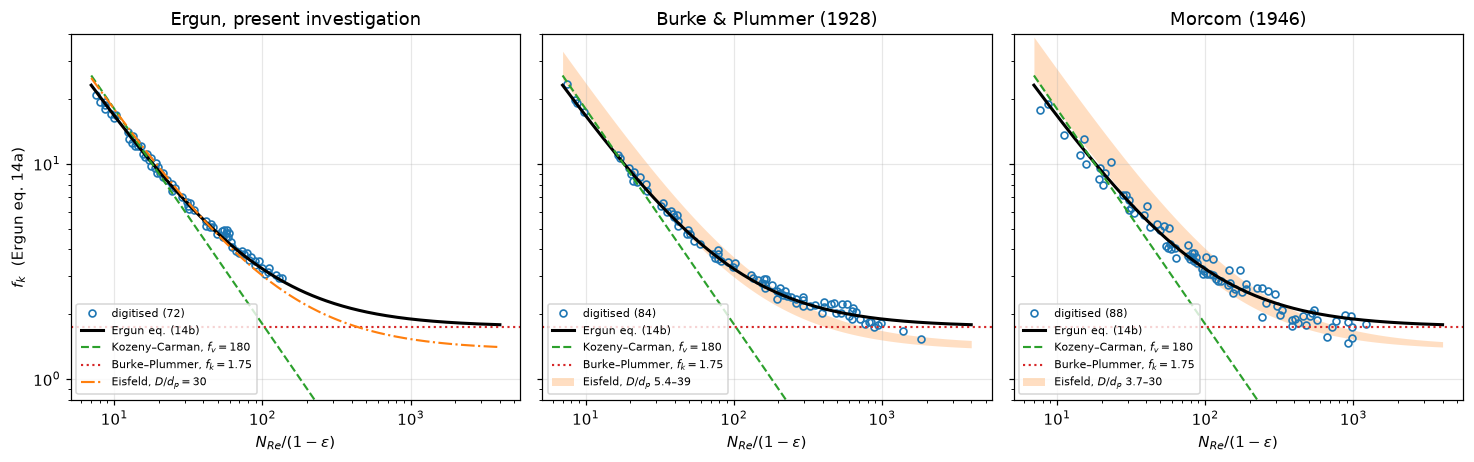
Ergun's own eq. (13c) against the 244 points he drew it through:
   bias +0.35 %   mean |dev|  5.16 %   rms  7.13 %
   (deviation = (model - measured)/measured, throughout)

scatter about Ergun's line, panel by panel (rms of the deviation):
   burke_plummer           5.10 %
   morcom                 10.18 %
   present_investigation   3.92 %
largest: morcomTrueWhere the four actually differ
On log axes everything looks like agreement. The honest picture is the ratio.
fig, axes = plt.subplots(1, 2, figsize=(12.2, 4.3))

ax = axes[0]
ax.loglog(xx, ergun_fv(xx), "k-", lw=2.0, label="Ergun")
ax.loglog(xx, kozeny_carman_fv(xx), "--", lw=1.6, color="tab:green",
          label=f"Kozeny–Carman ({KC_FV:g})")
ax.loglog(xx, eisfeld_fv(xx, EPS, D_INF), "-.", lw=1.6, color="tab:orange",
          label=r"Eisfeld, $D/d_p\to\infty$")
ax.loglog(xx, eisfeld_fv(xx, EPS, 5.0), ":", lw=1.8, color="tab:orange",
          label=r"Eisfeld, $D/d_p=5$")
ax.loglog(x, f_v, ".", ms=3, color="tab:blue", alpha=0.55,
          label=f"Ergun's data ({len(x)})")
ax.set(xlabel=r"$N_{Re}/(1-\epsilon)$", ylabel=r"$f_v$",
       title="the linear form Ergun fitted in")
ax.legend(fontsize=8, loc="upper left")

ax = axes[1]
base = ergun_fv(xx)
ax.semilogx(xx, kozeny_carman_fv(xx) / base - 1, "--", lw=1.6,
            color="tab:green", label="Kozeny–Carman")
ax.semilogx(xx, eisfeld_fv(xx, EPS, D_INF) / base - 1, "-.", lw=1.6,
            color="tab:orange", label=r"Eisfeld, $D/d_p\to\infty$")
for r, ls in ((20.0, (0, (4, 2))), (10.0, (0, (2, 2))), (5.0, ":")):
    ax.semilogx(xx, eisfeld_fv(xx, EPS, r) / base - 1, ls=ls, lw=1.6,
                color="tab:purple", label=rf"Eisfeld, $D/d_p={r:g}$")
ax.axhline(0, color="k", lw=1.6)
ax.axhspan(-mad_e, mad_e, color="tab:blue", alpha=0.12, lw=0)
ax.set(xlabel=r"$N_{Re}/(1-\epsilon)$",
       ylabel="(correlation $-$ Ergun) / Ergun", ylim=(-0.55, 0.85),
       title="divergence from Ergun, with his own scatter shaded")
ax.legend(fontsize=8, ncol=2)
fig.tight_layout()
plt.show()


def vs_ergun(model_fv, xq):
    """(correlation - Ergun) / Ergun at N_Re/(1-eps) = xq."""
    return float(model_fv / ergun_fv(xq) - 1)


XQ = (10, 100, 1000)
for xq in XQ:
    e = float(ergun_fv(xq))
    print(f"at N_Re/(1-eps) = {xq:5d}:  Ergun {e:8.1f}"
          f"   K–C {vs_ergun(kozeny_carman_fv(xq), xq):+7.1%}"
          f"   Eisfeld(inf) {vs_ergun(eisfeld_fv(xq, EPS, D_INF), xq):+7.1%}"
          f"   Eisfeld(D/d=5) {vs_ergun(eisfeld_fv(xq, EPS, 5.0), xq):+7.1%}")
    claims.value(f"kc_vs_ergun_x{xq}", vs_ergun(kozeny_carman_fv(xq), xq), rtol=0.05)
    claims.value(f"eis_inf_vs_ergun_x{xq}", vs_ergun(eisfeld_fv(xq, EPS, D_INF), xq), rtol=0.05)
    claims.value(f"eis_r5_vs_ergun_x{xq}", vs_ergun(eisfeld_fv(xq, EPS, 5.0), xq), rtol=0.05)
    brk(f"Kozeny-Carman with k = 4 in place of {KC_K:g}", f"kc_vs_ergun_x{xq}",
        vs_ergun(kozeny_carman_fv(xq, k=4.0), xq))
    brk(f"Eisfeld's cylinder coefficients (K1 = {EIS_CYL['K1']:g}, k1 = {EIS_CYL['k1']:g}, k2 = {EIS_CYL['k2']:g})",
        f"eis_inf_vs_ergun_x{xq}", vs_ergun(eisfeld_fv(xq, EPS, D_INF, **EIS_CYL), xq))
    brk(f"Kozeny-Carman with k = 10 in place of {KC_K:g}", f"kc_vs_ergun_x{xq}",
        vs_ergun(kozeny_carman_fv(xq, k=10.0), xq))
    brk("Eisfeld at D/d_p = 10 in place of 5", f"eis_r5_vs_ergun_x{xq}",
        vs_ergun(eisfeld_fv(xq, EPS, 10.0), xq))

# the two asymptotes of Eisfeld's infinite-bed form against Ergun's constants
VISC_EIS_ERGUN = EIS["K1"] / K1_ERGUN - 1
INERT_EIS_ERGUN = b_inf / K2_ERGUN - 1
claims.value("eis_viscous_vs_ergun", VISC_EIS_ERGUN, rtol=0.05)
claims.value("eis_inertial_vs_ergun", INERT_EIS_ERGUN, rtol=0.05)
brk("Eisfeld's cylinder coefficient K1", "eis_viscous_vs_ergun", EIS_CYL["K1"] / K1_ERGUN - 1)
brk("Eisfeld's cylinder coefficient k2", "eis_inertial_vs_ergun",
    eisfeld_coeffs(EPS, D_INF, **EIS_CYL)[1] / K2_ERGUN - 1)

# Kozeny-Carman: where it is right
kc0 = vs_ergun(kozeny_carman_fv(0.0), 0.0)
kc3 = vs_ergun(kozeny_carman_fv(3.0), 3.0)


def kc_window(tol, k=KC_K):
    """N_Re/(1-eps) at which Kozeny-Carman is `tol` above (+) or below (-) Ergun."""
    return (36.0 * k / (1.0 + tol) - K1_ERGUN) / K2_ERGUN


KC_LO, KC_HI = kc_window(+0.10), kc_window(-0.10)
claims.value("kc_vs_ergun_creeping", kc0, rtol=0.05)
claims.value("kc_vs_ergun_x3", kc3, rtol=0.05)
claims.value("kc_within_10pct_lo", KC_LO, rtol=0.05)
claims.value("kc_within_10pct_hi", KC_HI, rtol=0.05)
brk("Kozeny-Carman with k = 4", "kc_vs_ergun_creeping", vs_ergun(kozeny_carman_fv(0.0, k=4.0), 0.0))
brk("Kozeny-Carman with k = 4", "kc_vs_ergun_x3", vs_ergun(kozeny_carman_fv(3.0, k=4.0), 3.0))
brk(f"Carman's constant {KC_FV:g} 5 % low (k = {KC_K * 0.95:g})", "kc_within_10pct_lo", kc_window(+0.10, k=KC_K * 0.95))
brk("Kozeny-Carman with k = 4", "kc_within_10pct_hi", kc_window(-0.10, k=4.0))
display(Markdown(rf"""
**Kozeny–Carman is not "right in creeping flow" against Ergun's equation.** It is
{kc0:+.1%} above it as $x \to 0$ and {kc3:+.1%} at $x = 3$, because its constant
({KC_FV:g}) is not Ergun's ({K1_ERGUN:g}); it is within 10 % of Ergun only for
$x$ between {KC_LO:.1f} and {KC_HI:.1f}.
"""))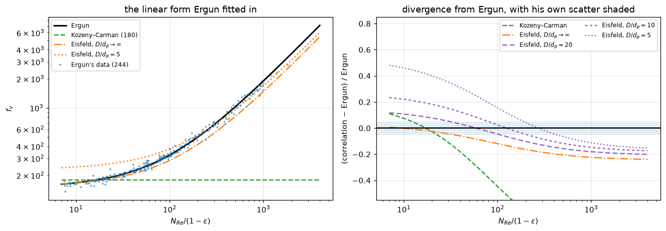
at N_Re/(1-eps) =    10:  Ergun    167.5   K–C   +7.5%   Eisfeld(inf)   -0.2%   Eisfeld(D/d=5)  +46.0%
at N_Re/(1-eps) =   100:  Ergun    325.0   K–C  -44.6%   Eisfeld(inf)  -12.0%   Eisfeld(D/d=5)  +15.6%
at N_Re/(1-eps) =  1000:  Ergun   1900.0   K–C  -90.5%   Eisfeld(inf)  -22.4%   Eisfeld(D/d=5)  -11.2%
Kozeny–Carman is not “right in creeping flow” against Ergun’s equation. It is +20.0% above it as \(x \to 0\) and +15.9% at \(x = 3\), because its constant (180) is not Ergun’s (150); it is within 10 % of Ergun only for \(x\) between 7.8 and 28.6.
The wall-effect regime
The correction is not monotone in Reynolds number, and that is the whole point of Eisfeld & Schnitzlein’s paper: “the wall effect is predicted to increase the pressure drop at low and moderate Reynolds numbers; only for sufficiently high \(Re_{d_p}\) values and for very small tube-to-particle diameter ratios a pressure drop reduction is obtained.” Wall friction and the looser near-wall packing pull opposite ways, and which wins depends on the flow regime.
The shaded bands are where the sources Ergun plotted actually sit.
ratios = np.logspace(np.log10(1.624), np.log10(250), 400)
fig, ax = plt.subplots(figsize=(8.2, 4.8))
for xq, col in zip((3, 30, 300, 3000, 30000),
                   plt.cm.viridis(np.linspace(0.10, 0.90, 5))):
    ax.semilogx(ratios, eisfeld_fv(xq, EPS, ratios)
                / eisfeld_fv(xq, EPS, D_INF) - 1, color=col, lw=2.0,
                label=rf"$N_{{Re}}/(1-\epsilon) = {xq}$")
ax.axhline(0, color="k", lw=1.2)
for key, col, ytxt in (("morcom", "tab:red", 1.02),
                       ("burke_plummer", "tab:blue", 0.90)):
    lo, hi = PANEL[key]["D_over_dp"]
    ax.axvspan(lo, hi, color=col, alpha=0.09, lw=0)
    ax.plot([lo, hi], [ytxt, ytxt], lw=3, color=col, alpha=0.7,
            solid_capstyle="butt")
    ax.text(hi * 1.15, ytxt, PANEL[key]["label"].split(" (")[0],
            va="center", fontsize=8, color=col)
ax.axvline(10, color="grey", lw=1.0, ls="--")
ax.text(10.4, -0.30, r"$D/d_p=10$: Ergun's own cut" "\n" "for Burke & Plummer",
        fontsize=7.5, color="grey")
ax.set(xlabel=r"tube-to-particle diameter ratio $D/d_p$",
       ylabel="wall correction on $f_v$, relative to an infinite bed",
       title=rf"Eisfeld & Schnitzlein eq. (3), $\epsilon={EPS:g}$",
       ylim=(-0.45, 1.15), xlim=(1.5, 300))
ax.legend(fontsize=8, loc="center right")
fig.tight_layout()
plt.show()

print("Eisfeld & Schnitzlein, Table 1, for the sources Ergun plotted:")
print(src[["source", "particles", "n_data", "D_over_dp_min", "D_over_dp_max",
           "ergun_fig7_panel"]].fillna("-").to_string(index=False))


def morcom_range(exclude=("cylinders",)):
    """D/d_p range of Morcom's packings in Table 1, leaving out the named particles."""
    m = src[(src.source.str.startswith("Morcom")) & (~src.particles.isin(exclude))]
    return float(m.D_over_dp_min.min()), float(m.D_over_dp_max.max())


MORCOM_LO, MORCOM_HI = morcom_range()
CYL_HI = morcom_range(exclude=())[1]
BP_LO = float(src[src.ergun_fig7_panel == "burke_plummer"].D_over_dp_min.min())
claims.value("morcom_noncyl_Dp_min", MORCOM_LO, rtol=0.05)
claims.value("morcom_noncyl_Dp_max", MORCOM_HI, rtol=0.05)
claims.value("morcom_cylinders_Dp_max", CYL_HI, rtol=0.05)
claims.value("burke_plummer_Dp_min", BP_LO, rtol=0.05)
claims.says("5.4", "burke_plummer_Dp_min")     # "honest limits" text below
brk("Morcom's cylinders counted with the rest", "morcom_noncyl_Dp_max", morcom_range(exclude=())[1])
brk("Morcom's spheres and tablets left out", "morcom_noncyl_Dp_min", morcom_range(exclude=("spheres", "tablets"))[0])
brk("Burke & Plummer's range read from Ergun and Orning's row", "burke_plummer_Dp_min",
    float(src[src.source.str.startswith("Ergun and Orning")].D_over_dp_min.min()))
brk("the cylinders' lower end", "morcom_cylinders_Dp_max", float(src[src.particles == "cylinders"].D_over_dp_min.min()))
print(f"\nMorcom's spheres, tablets and nodules sit at D/d_p = {MORCOM_LO:.1f}-{MORCOM_HI:.1f}; only his")
print(f"cylinders reach {CYL_HI:.1f}. On Ergun's own criterion - he dropped the Burke &")
print(f"Plummer systems below D/d_p = 10 - most of that panel is inside the")
print("wall-effect regime, and he kept it. Eisfeld's Burke & Plummer row itself")
print(f"reaches down to D/d_p = {BP_LO:.1f}.")

R_SMALL = float(eis[eis.quantity == "D_over_dp_min"].value.iloc[0])      # smallest D/d_p of the 2391 points
print(f"\nAt the small-D/d_p end (D/d_p = {R_SMALL:g}) the correction changes sign with flow regime:")


def wall_corr(xq, r, eps=EPS, **kw):
    """Wall correction on f_v at tube-to-particle ratio r, relative to an infinite bed."""
    return float(eisfeld_fv(xq, eps, r, **kw) / eisfeld_fv(xq, eps, D_INF, **kw) - 1)


for xq in (3, 300, 30000):
    print(f"   D/d_p = {R_SMALL:g}, N_Re/(1-eps) = {xq:6d}: {wall_corr(xq, R_SMALL):+7.1%}")
    claims.value(f"wall_corr_smallest_x{xq}", wall_corr(xq, R_SMALL), rtol=0.05)
    brk("D/d_p = 3 in place of the smallest ratio", f"wall_corr_smallest_x{xq}", wall_corr(xq, 3.0))
print("   which is the counteracting pair Eisfeld & Schnitzlein describe -")
print("   wall friction raising the viscous term, looser near-wall packing")
print("   lowering the inertial one.")

# How big is the wall correction next to the gaps between the correlations?
R_WALL = 5.0


def gap_ergun_eis(xq, **kw):
    """Eisfeld's infinite-bed form against Ergun, relative."""
    return vs_ergun(eisfeld_fv(xq, EPS, D_INF, **kw), xq)


def wall_beats_gap(r, other="eisfeld", **kw):
    """Largest x (in 10..1e4) up to which the wall correction at D/d_p = r is larger
    than the gap between Ergun and `other` (Eisfeld infinite-bed form, or Kozeny-Carman)."""
    gap = (lambda q: abs(gap_ergun_eis(q, **kw))) if other == "eisfeld" else \
          (lambda q: abs(vs_ergun(kozeny_carman_fv(q), q)))
    f = lambda lq: abs(wall_corr(10 ** lq, r, **kw)) - gap(10 ** lq)
    grid = np.linspace(1.0, 4.0, 301)
    s = np.sign([f(g) for g in grid])
    flips = np.where(s[:-1] * s[1:] < 0)[0]
    if flips.size == 0:
        return float("nan") if s[0] < 0 else float(10 ** grid[-1])
    i = flips[0]
    return float(10 ** brentq(f, grid[i], grid[i + 1], xtol=1e-12))


XW = {o: wall_beats_gap(R_WALL, o) for o in ("eisfeld", "kc")}


def round_sig(v, n=2):
    """v to n significant digits."""
    return float(f"{v:.{n - 1}e}")


XW_EIS_ROUND = round_sig(XW["eisfeld"])
for xq in XQ:
    claims.value(f"wall_corr_r5_x{xq}", wall_corr(xq, R_WALL), rtol=0.05)
    brk("D/d_p = 10 in place of 5", f"wall_corr_r5_x{xq}", wall_corr(xq, 10.0))
claims.value("wall_beats_eis_gap_x_max", XW["eisfeld"], rtol=0.05)
claims.value("wall_beats_kc_gap_x_max", XW["kc"], rtol=0.05)
brk("D/d_p = 10 in place of 5", "wall_beats_eis_gap_x_max", wall_beats_gap(10.0, "eisfeld"))
brk("D/d_p = 10 in place of 5", "wall_beats_kc_gap_x_max", wall_beats_gap(10.0, "kc"))
display(Markdown(rf"""
**How large is the wall correction next to the gaps between the correlations?**
At $D/d_p$ = {R_WALL:g} it is {wall_corr(10, R_WALL):+.1%}, {wall_corr(100, R_WALL):+.1%} and
{wall_corr(1000, R_WALL):+.1%} at $x$ = 10, 100 and 1000. That is larger than the gap
between Ergun and Eisfeld's infinite-bed form ({gap_ergun_eis(10):+.1%}, {gap_ergun_eis(100):+.1%},
{gap_ergun_eis(1000):+.1%}) only up to $x$ of about {XW_EIS_ROUND:.0f}, and larger than the gap to
Kozeny–Carman ({vs_ergun(kozeny_carman_fv(10), 10):+.1%}, {vs_ergun(kozeny_carman_fv(100), 100):+.1%},
{vs_ergun(kozeny_carman_fv(1000), 1000):+.1%}) only up to $x$ = {XW['kc']:.0f}. So at $D/d_p$ = {R_WALL:g} the wall
matters as much as the choice between correlations at low and moderate Reynolds number, and
less than it at high Reynolds number.
"""))

# sign change of the wall correction
def r_sign_change(eps=EPS):
    """D/d_p below which Eisfeld's inertial coefficient falls under its infinite-bed value
    (so that the wall correction on f_v changes sign at high enough x)."""
    f = lambda lr: eisfeld_coeffs(eps, 10 ** lr)[1] / eisfeld_coeffs(eps, D_INF)[1] - 1
    return float(10 ** brentq(f, np.log10(R_SMALL), 2.0, xtol=1e-12))


R_SIGN = r_sign_change()
claims.value("wall_sign_change_Dp", R_SIGN, rtol=0.05)
brk("voidage 0.60 in place of 0.40", "wall_sign_change_Dp", r_sign_change(0.60))
print(f"   the inertial coefficient, and with it the sign of the correction at high x, falls below its")
print(f"   infinite-bed value only for D/d_p < {R_SIGN:.2f}")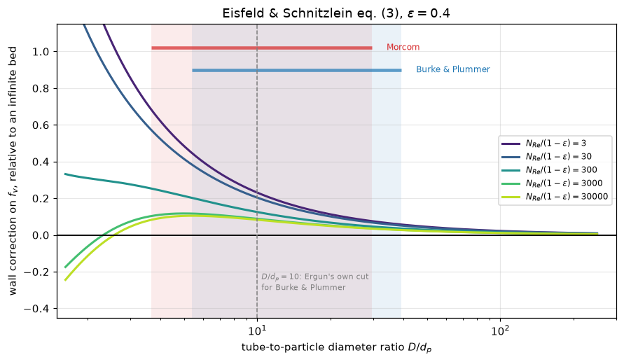
Eisfeld & Schnitzlein, Table 1, for the sources Ergun plotted:
                  source particles  n_data  D_over_dp_min  D_over_dp_max ergun_fig7_panel
Burke and Plummer (1928)   spheres     219          5.379         39.179    burke_plummer
 Ergun and Orning (1949)   spheres      53         44.561         51.107                -
           Morcom (1946)   spheres      15          3.663          6.607           morcom
           Morcom (1946)   nodules       3         10.569         10.569           morcom
           Morcom (1946)   tablets      26          5.778          9.110           morcom
           Morcom (1946) cylinders      28          9.566         29.613           morcom
  Oman and Watson (1944)  granules      31         35.059         35.119                -
  Oman and Watson (1944)   spheres      30         18.446         18.642                -
  Oman and Watson (1944) cylinders      22         13.801         13.863                -

Morcom's spheres, tablets and nodules sit at D/d_p = 3.7-10.6; only his
cylinders reach 29.6. On Ergun's own criterion - he dropped the Burke &
Plummer systems below D/d_p = 10 - most of that panel is inside the
wall-effect regime, and he kept it. Eisfeld's Burke & Plummer row itself
reaches down to D/d_p = 5.4.

At the small-D/d_p end (D/d_p = 1.624) the correction changes sign with flow regime:
   D/d_p = 1.624, N_Re/(1-eps) =      3: +178.4%
   D/d_p = 1.624, N_Re/(1-eps) =    300:  +33.2%
   D/d_p = 1.624, N_Re/(1-eps) =  30000:  -24.5%
   which is the counteracting pair Eisfeld & Schnitzlein describe -
   wall friction raising the viscous term, looser near-wall packing
   lowering the inertial one.
How large is the wall correction next to the gaps between the correlations? At \(D/d_p\) = 5 it is +46.3%, +31.3% and +14.3% at \(x\) = 10, 100 and 1000. That is larger than the gap between Ergun and Eisfeld’s infinite-bed form (-0.2%, -12.0%, -22.4%) only up to \(x\) of about 380, and larger than the gap to Kozeny–Carman (+7.5%, -44.6%, -90.5%) only up to \(x\) = 71. So at \(D/d_p\) = 5 the wall matters as much as the choice between correlations at low and moderate Reynolds number, and less than it at high Reynolds number.
   the inertial coefficient, and with it the sign of the correction at high x, falls below its
   infinite-bed value only for D/d_p < 2.61
A design number: an isothermal compressible bed
The closures matter because they are the source term of a momentum balance. For an ideal gas at fixed mass flux both Ergun terms scale as \(1/p\), so \(p\,\mathrm{d}p/\mathrm{d}z = -K\) with \(K = (RT/M)\,[A (1-\epsilon)^2 \mu G/(\epsilon^3 d_p^2) + B (1-\epsilon) G^2/(\epsilon^3 d_p)]\) and \(p(z) = \sqrt{p_{in}^2 - 2Kz}\) exactly. The two-route check is the point: the closed form and a direct ODE integration of \(\mathrm{d}p/\mathrm{d}z = -K/p\) are independent, and must agree.
BED = dict(T=300.0, M=0.029, mu=1.85e-5, dp=3e-3, eps=0.40, L=2.0, p_in=2e5)


def bed_K(A, B, G, **bed):
    """K in p dp/dz = -K for an ideal gas at mass flux G; `bed` overrides BED."""
    b = {**BED, **bed}
    return (R_GAS * b["T"] / b["M"]) * (
        A * (1 - b["eps"]) ** 2 * b["mu"] * G / (b["eps"] ** 3 * b["dp"] ** 2)
        + B * (1 - b["eps"]) * G ** 2 / (b["eps"] ** 3 * b["dp"]))


def outlet_pressure(A, B, G, **bed):
    """Closed-form outlet pressure sqrt(p_in^2 - 2 K L)."""
    b = {**BED, **bed}
    return np.sqrt(b["p_in"] ** 2 - 2 * bed_K(A, B, G, **bed) * b["L"])


def outlet_pressure_ode(A, B, G, G_ode=None, rtol=1e-10, **bed):
    """Outlet pressure by integrating dp/dz = -K/p; `G_ode` injects a wrong flux."""
    b = {**BED, **bed}
    K = bed_K(A, B, G if G_ode is None else G_ode, **bed)
    sol = solve_ivp(lambda z, p: -K / p, (0.0, b["L"]), [b["p_in"]],
                    rtol=rtol, atol=1e-6)
    return float(sol.y[0, -1])


G_REF = 1.0   # kg/(m2 s)
two_routes = abs(outlet_pressure_ode(K1_ERGUN, K2_ERGUN, G_REF)
                 / outlet_pressure(K1_ERGUN, K2_ERGUN, G_REF) - 1)
print(f"closed form  p_out = {outlet_pressure(K1_ERGUN, K2_ERGUN, G_REF):.4f} Pa")
print(f"solve_ivp    p_out = {outlet_pressure_ode(K1_ERGUN, K2_ERGUN, G_REF):.4f} Pa")
print(f"two independent routes agree below 1e-9 (here {two_routes:.1e}), solve_ivp rtol 1e-10")
claims.bound("bed_two_routes_rel", two_routes, max=1e-9, basis="tolerance",
             note="solve_ivp rtol 1e-10")
brk(f"the ODE integrated at G = 1.01 in place of {G_REF:g}", "bed_two_routes_rel",
    abs(outlet_pressure_ode(K1_ERGUN, K2_ERGUN, G_REF, G_ode=1.01 * G_REF)
        / outlet_pressure(K1_ERGUN, K2_ERGUN, G_REF) - 1))

# Stop the sweep before the bed would need more head than the inlet has:
# 2 K(G) L = p_in^2 with K = c1 G + c2 G^2 is a quadratic in G.
c1 = bed_K(K1_ERGUN, 0.0, 1.0)
c2 = bed_K(0.0, K2_ERGUN, 1.0)
G_max = (-c1 + np.sqrt(c1 ** 2 + 4 * c2 * BED["p_in"] ** 2 / (2 * BED["L"]))) \
    / (2 * c2)
Gs = np.logspace(-1.5, np.log10(0.85 * G_max), 60)

fig, axes = plt.subplots(1, 2, figsize=(12.2, 4.3))
for ax, ratio, ttl in zip(axes, (40.0, 5.0),
                          (r"a wide tube, $D/d_p=40$",
                           r"a narrow tube, $D/d_p=5$")):
    curves = (("Ergun", (K1_ERGUN, K2_ERGUN), "k", "-"),
              ("Kozeny–Carman", (KC_FV, 0.0), "tab:green", "--"),
              ("Eisfeld", eisfeld_coeffs(EPS, ratio), "tab:orange", "-."))
    for nm, (A, B), col, ls in curves:
        dp_bar = (BED["p_in"] - outlet_pressure(A, B, Gs)) / 1e5
        ax.loglog(Gs * BED["dp"] / BED["mu"], dp_bar, ls=ls, color=col,
                  lw=1.8, label=nm)
    ax.set(xlabel=r"$Re_{d_p} = G d_p/\mu$",
           ylabel=r"$\Delta p$ over 2 m  [bar]", title=ttl)
    ax.legend(fontsize=8)
fig.tight_layout()
plt.show()


def bed_drop_kpa(coeffs, G=G_REF, **bed):
    """Pressure drop over the bed in kPa for (A, B) = coeffs."""
    b = {**BED, **bed}
    return float((b["p_in"] - outlet_pressure(*coeffs, G, **bed)) / 1e3)


CASES = {"Ergun": (K1_ERGUN, K2_ERGUN),
         "Kozeny–Carman": (KC_FV, 0.0),
         "Eisfeld, D/d_p = infinity": eisfeld_coeffs(EPS, D_INF),
         "Eisfeld, D/d_p = 40": eisfeld_coeffs(EPS, 40.0),
         "Eisfeld, D/d_p = 5": eisfeld_coeffs(EPS, 5.0)}
print(f"outlet pressure after {BED['L']:g} m, air at {BED['T']:g} K, {BED['dp']*1e3:g} mm particles, "
      f"eps = {BED['eps']:g},")
print(f"inlet {BED['p_in']/1e5:.1f} bar, G = {G_REF:g} kg/(m2 s)  "
      f"(Re_dp = {G_REF*BED['dp']/BED['mu']:.0f}):")
for nm, co in CASES.items():
    print(f"   {nm:26s} dp = {bed_drop_kpa(co):5.2f} kPa   "
          f"p_out = {BED['p_in']/1e3 - bed_drop_kpa(co):6.2f} kPa")
    key = {"Ergun": "ergun", "Kozeny–Carman": "kc", "Eisfeld, D/d_p = infinity": "eis_inf",
           "Eisfeld, D/d_p = 40": "eis_r40", "Eisfeld, D/d_p = 5": "eis_r5"}[nm]
    claims.value(f"bed_dp_kpa_{key}", bed_drop_kpa(co), rtol=0.05)
    brk(f"particle diameter {1.1*BED['dp']*1e3:.1f} mm in place of {BED['dp']*1e3:g} mm",
        f"bed_dp_kpa_{key}", bed_drop_kpa(co, dp=1.1 * BED["dp"]))

RE_DP = G_REF * BED["dp"] / BED["mu"]
visc5, inert5 = eisfeld_coeffs(EPS, 5.0)
VISC_RISE, INERT_RISE = visc5 / a_inf - 1, inert5 / b_inf - 1
claims.value("wall_r5_viscous_coeff_change", VISC_RISE, rtol=0.05)
claims.value("wall_r5_inertial_coeff_change", INERT_RISE, rtol=0.05)
visc10, inert10 = eisfeld_coeffs(EPS, 10.0)
brk("D/d_p = 10 in place of 5", "wall_r5_viscous_coeff_change", visc10 / a_inf - 1)
brk("D/d_p = 10 in place of 5", "wall_r5_inertial_coeff_change", inert10 / b_inf - 1)


def wall_dp_effect(G, r=5.0, **kw):
    """Pressure drop with the wall at D/d_p = r, relative to Eisfeld's infinite bed."""
    return bed_drop_kpa(eisfeld_coeffs(EPS, r, **kw), G) / bed_drop_kpa(eisfeld_coeffs(EPS, D_INF, **kw), G) - 1


G_LADDER = (G_REF, G_REF / 10, G_REF / 100)
for G_ in G_LADDER:
    claims.value(f"wall_dp_effect_G{G_:g}", wall_dp_effect(G_), rtol=0.05)
    brk("D/d_p = 10 in place of 5", f"wall_dp_effect_G{G_:g}", wall_dp_effect(G_, 10.0))
EIS_INF_VS_ERGUN_DP = bed_drop_kpa(CASES["Eisfeld, D/d_p = infinity"]) / bed_drop_kpa(CASES["Ergun"]) - 1
claims.value("bed_dp_eis_inf_vs_ergun", EIS_INF_VS_ERGUN_DP, rtol=0.05)
brk("Eisfeld's cylinder coefficients", "bed_dp_eis_inf_vs_ergun",
    bed_drop_kpa(eisfeld_coeffs(EPS, D_INF, **EIS_CYL)) / bed_drop_kpa(CASES["Ergun"]) - 1)

display(Markdown(rf"""
**The wall's two effects do not cancel here, they add.** At $D/d_p$ = 5 the wall
raises the viscous coefficient by {VISC_RISE:.1%} and the inertial one by
{INERT_RISE:.1%} relative to Eisfeld's infinite bed, so the pressure drop at
$Re_{{d_p}}$ = {RE_DP:.0f} is {wall_dp_effect(G_REF):+.1%} above the same
correlation's infinite bed; it is {wall_dp_effect(G_REF/10):+.1%} at a tenth of the
flux and {wall_dp_effect(G_REF/100):+.1%} at a hundredth. That the $D/d_p$ = 5 value
({bed_drop_kpa(CASES['Eisfeld, D/d_p = 5']):.2f} kPa) lands on Ergun's
({bed_drop_kpa(CASES['Ergun']):.2f} kPa) is a coincidence of two opposite
differences: Eisfeld's infinite-bed form is {EIS_INF_VS_ERGUN_DP:+.1%} from Ergun's
at this flow. The correction changes sign with flow regime only below
$D/d_p$ = {R_SIGN:.2f} (previous section), so at $D/d_p$ = 5 it is a pure increase.
"""))
closed form p_out = 193705.4166 Pa
solve_ivp p_out = 193705.4166 Pa
two independent routes agree below 1e-9 (here 1.7e-14), solve_ivp rtol 1e-10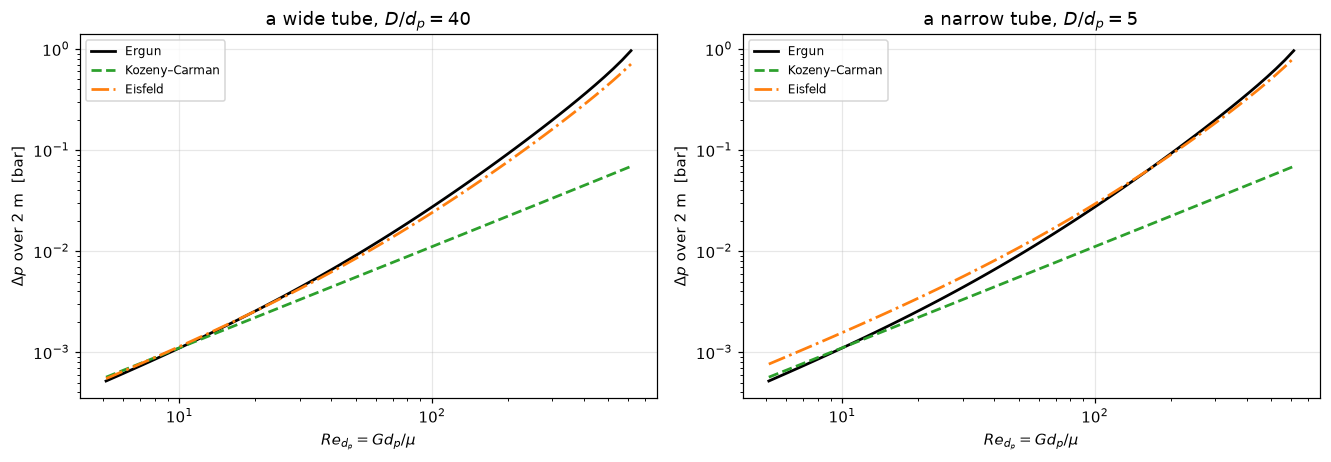
outlet pressure after 2 m, air at 300 K, 3 mm particles, eps = 0.4,
inlet 2.0 bar, G = 1 kg/(m2 s)  (Re_dp = 162):
   Ergun                      dp =  6.29 kPa   p_out = 193.71 kPa
   Kozeny–Carman              dp =  1.80 kPa   p_out = 198.20 kPa
   Eisfeld, D/d_p = infinity  dp =  5.15 kPa   p_out = 194.85 kPa
   Eisfeld, D/d_p = 40        dp =  5.33 kPa   p_out = 194.67 kPa
   Eisfeld, D/d_p = 5         dp =  6.30 kPa   p_out = 193.70 kPa
The wall’s two effects do not cancel here, they add. At \(D/d_p\) = 5 the wall raises the viscous coefficient by 49.4% and the inertial one by 10.3% relative to Eisfeld’s infinite bed, so the pressure drop at \(Re_{d_p}\) = 162 is +22.4% above the same correlation’s infinite bed; it is +42.0% at a tenth of the flux and +48.5% at a hundredth. That the \(D/d_p\) = 5 value (6.30 kPa) lands on Ergun’s (6.29 kPa) is a coincidence of two opposite differences: Eisfeld’s infinite-bed form is -18.2% from Ergun’s at this flow. The correction changes sign with flow regime only below \(D/d_p\) = 2.61 (previous section), so at \(D/d_p\) = 5 it is a pure increase.
Validation
Seven checks. The first is the one the paper pays for: Ergun’s constants were fitted to these points, so refitting them has to give 150 and 1.75 back.
def fit_forchheimer(x, fv, power=1.0):
    """Least squares on f_v = A + B x, with weight 1/f_v**power.

    The weighting is not cosmetic. f_v spans two and a half decades here, so an
    unweighted fit (power = 0) in these coordinates is dominated by a handful of
    high-Re points; equal RELATIVE weight (power = 1) is what "least squares"
    has to mean when the data are read off log axes."""
    x = np.asarray(x, float); fv = np.asarray(fv, float)
    A = np.vstack([np.ones_like(x), x]).T
    w = fv ** -power
    return np.linalg.lstsq(A * w[:, None], fv * w, rcond=None)[0]


def panel_fits(o, power=1.0, ordinate="f_v"):
    """(k1, k2) refit per series of a digitised table; `ordinate` names the column fitted."""
    return {s: tuple(fit_forchheimer(g.Re_over_one_minus_eps, g[ordinate], power))
            for s, g in o.groupby("series")}


print("1. Refit Ergun's two constants from his own figure")
A_all, B_all = fit_forchheimer(x, f_v)
print(f"   all {len(x)} points   k1 = {A_all:7.2f}  ({A_all/K1_ERGUN-1:+.1%})"
      f"     k2 = {B_all:6.3f}  ({B_all/K2_ERGUN-1:+.1%})")
print(f"   Ergun printed  k1 = {K1_ERGUN:7.2f}                 "
      f"k2 = {K2_ERGUN:6.3f}")
claims.value("k1_refit_all_points", A_all, rtol=0.05)
claims.value("k2_refit_all_points", B_all, rtol=0.05)
claims.value("k1_relative_error", A_all / K1_ERGUN - 1, rtol=0.05)
claims.value("k2_relative_error", B_all / K2_ERGUN - 1, rtol=0.05)
A_u, B_u = fit_forchheimer(x, f_v, power=0.0)
brk("the fit left unweighted (weight exponent 0)", "k1_refit_all_points", A_u)
brk("the fit left unweighted (weight exponent 0)", "k1_relative_error", A_u / K1_ERGUN - 1)
brk("only the present-investigation panel fitted", "k2_refit_all_points",
    panel_fits(obs)["present_investigation"][1])
brk("only the present-investigation panel fitted", "k2_relative_error",
    panel_fits(obs)["present_investigation"][1] / K2_ERGUN - 1)

print("\n   and independently, panel by panel - three sources, three separate")
print("   axis calibrations, no shared arithmetic:")
per_panel = panel_fits(obs)
for s, g in obs.groupby("series"):
    a, b = per_panel[s]
    print(f"      {s:22s} n={len(g):3d}   k1 = {a:6.2f}   k2 = {b:5.3f}")
    claims.value(f"k1_panel_{s}", a, rtol=0.05)
    claims.value(f"k2_panel_{s}", b, rtol=0.05)
    brk("the panel fit left unweighted", f"k1_panel_{s}", panel_fits(obs, power=0.0)[s][0])
    brk("Fig. 7's f_k fitted as if it were f_v (ordinates confused)", f"k1_panel_{s}",
        panel_fits(obs, ordinate="f_k")[s][0])
    brk("Fig. 7's f_k fitted as if it were f_v (ordinates confused)", f"k2_panel_{s}",
        panel_fits(obs, ordinate="f_k")[s][1])


def k1_spread(fits):
    """Half the range of k1 over the panels, relative to its mean."""
    k1s = np.array([v[0] for v in fits.values()])
    return float(np.ptp(k1s) / 2 / k1s.mean())


k1s = np.array([v[0] for v in per_panel.values()])
print(f"   spread in k1 across the three panels: "
      f"{k1s.min():.1f} to {k1s.max():.1f}, i.e. +/-{k1_spread(per_panel):.1%}")
claims.value("k1_panel_spread", k1_spread(per_panel), rtol=0.05)
claims.says("3 %", "k1_panel_spread")          # "honest limits" text below
brk("the panel fits left unweighted", "k1_panel_spread", k1_spread(panel_fits(obs, power=0.0)))

print("\n   The weighting is a real choice, so here is the alternative:")
print(f"      unweighted   k1 = {A_u:6.2f} ({A_u/K1_ERGUN-1:+.1%})   "
      f"k2 = {B_u:5.3f} ({B_u/K2_ERGUN-1:+.1%})")
print(f"      1/f_v weight k1 = {A_all:6.2f} ({A_all/K1_ERGUN-1:+.1%})   "
      f"k2 = {B_all:5.3f} ({B_all/K2_ERGUN-1:+.1%})")
claims.value("k1_unweighted", A_u, rtol=0.05)
claims.value("k2_unweighted", B_u, rtol=0.05)
claims.value("k1_unweighted_relative_error", A_u / K1_ERGUN - 1, rtol=0.05)
brk("the 1/f_v weight applied", "k1_unweighted", A_all)
brk("the 1/f_v weight applied", "k2_unweighted", B_all)
brk("the 1/f_v weight applied", "k1_unweighted_relative_error", A_all / K1_ERGUN - 1)
print("   Unweighted, the top decade of f_v carries a hundred times the weight")
print("   of the bottom one, and k1 - which lives at the bottom - drifts. The")
print("   relative-weight fit is the one quoted; the other is shown so that the")
print("   round trip is not resting on a hidden choice.")
1. Refit Ergun's two constants from his own figure
all 244 points k1 = 151.94 (+1.3%) k2 = 1.697 (-3.0%)
Ergun printed k1 = 150.00 k2 = 1.750
and independently, panel by panel - three sources, three separate
axis calibrations, no shared arithmetic:
burke_plummer n= 84 k1 = 154.57 k2 = 1.731
morcom n= 88 k1 = 151.03 k2 = 1.639
present_investigation n= 72 k1 = 146.58 k2 = 1.884
spread in k1 across the three panels: 146.6 to 154.6, i.e. +/-2.7%
The weighting is a real choice, so here is the alternative:
unweighted k1 = 168.53 (+12.4%) k2 = 1.605 (-8.3%)
1/f_v weight k1 = 151.94 (+1.3%) k2 = 1.697 (-3.0%)
Unweighted, the top decade of f_v carries a hundred times the weight
of the bottom one, and k1 - which lives at the bottom - drifts. The
relative-weight fit is the one quoted; the other is shown so that the
round trip is not resting on a hidden choice.print("2. The round trip is not circular - the detector cannot see the drawn line")
g = obs[obs.series == "present_investigation"]
X_LINE_END = 4000.0 # where Ergun's eq. (14b) line ends on the panel (read off the figure)
def panel_x_max(o, series="present_investigation"):
"""Largest N_Re/(1-eps) at which a marker was recovered in a panel (all panels if None)."""
return float((o if series is None else o[o.series == series]).Re_over_one_minus_eps.max())
claims.value("present_panel_x_max", panel_x_max(obs), rtol=0.05)
claims.says("136", "present_panel_x_max") # "honest limits" text below
brk("all three panels pooled (the detector following the drawn line would not stop)", "present_panel_x_max",
panel_x_max(obs, None))
print(f" Ergun's eq. (14b) line is drawn across the whole panel, out to")
print(f" N_Re/(1-eps) = {X_LINE_END:g}. The markers stop at {panel_x_max(obs):.1f}.")
print(" Beyond that the panel contains the line, the grid and nothing else,")
print(" and the extraction returns zero points there. Detection keys on the")
print(" enclosed white interior of an open circle; a line has none.")
print(f" If the detector had been tracking the curve, this column would run")
print(f" to {X_LINE_END:g}.")
print("\n3. The same runs, digitised twice, on two different ordinates")
BINS = np.logspace(np.log10(7), np.log10(140), 9)
def cross_check(o5, g7, ordinate="f_v", min_pts=3):
"""Binned median f_v ratio, Fig. 7 over Fig. 5, for the present-investigation runs.
`ordinate` names the Fig. 7 column used as the numerator; bins with fewer than
`min_pts` markers in either figure are dropped."""
f5x, f5v = o5.Re_over_one_minus_eps.values, o5.f_v.values
f7x, f7v = g7.Re_over_one_minus_eps.values, g7[ordinate].values
rat, ctr, npts = [], [], []
for lo, hi in zip(BINS[:-1], BINS[1:]):
m5 = (f5x >= lo) & (f5x < hi)
m7 = (f7x >= lo) & (f7x < hi)
npts.append(min(m5.sum(), m7.sum()))
if m5.sum() >= min_pts and m7.sum() >= min_pts:
rat.append(np.median(f7v[m7]) / np.median(f5v[m5]))
ctr.append(np.log10(np.sqrt(lo * hi)))
rat, ctr = np.array(rat), np.array(ctr)
slope, icpt = np.polyfit(ctr, rat, 1)
res = rat - (slope * ctr + icpt)
se = np.sqrt(res @ res / (len(rat) - 2) / np.sum((ctr - ctr.mean()) ** 2))
return dict(rat=rat, mean=float(rat.mean()), std=float(rat.std()), n=len(rat),
slope=float(slope), se=float(se), t=float(slope / se), npts=np.array(npts))
CC = cross_check(obs5, g)
print(f" Fig. 5 top panel: {len(obs5)} markers, ordinate f_v, its own calibration")
print(f" Fig. 7 top panel: {len(g)} markers, ordinate f_k, its own calibration")
print(f" markers per bin (the smaller of the two figures): {CC['npts'].tolist()}")
print(" binned median f_v ratio, Fig. 7 / Fig. 5, per bin: "
+ " ".join(f"{r:.3f}" for r in CC["rat"]))
print(f" over {CC['n']} bins: {CC['mean']:.4f} +/- {CC['std']:.4f}")
print(f" trend with log10 x: {CC['slope']:+.4f} per decade, standard error {CC['se']:.4f}"
f" (t = {CC['t']:+.2f})")
print(f" -> the two independent readings of one set of runs agree to"
f" {abs(CC['mean']-1)*100:.1f} %, with no trend beyond its standard error")
print(" Point-by-point pairing is NOT attempted: in the dense chain two")
print(" markers can sit closer in x than the pairing tolerance, and a")
print(" mismatched pair inflates the scatter without meaning anything.")
claims.value("fig5_fig7_cross_check_ratio", CC["mean"], rtol=0.05)
claims.value("fig5_fig7_bin_scatter", CC["std"], rtol=0.05)
claims.bound("fig5_fig7_trend_t", abs(CC["t"]), max=2.0, basis="chosen",
note="|slope| of the bin ratio against log x within two standard errors")
n_bins_ok = claims.count("fig5_fig7_bins_used", CC["npts"], 2.5, min_margin=0.1)
brk("Fig. 7's f_k used as if it were f_v (ordinates confused)", "fig5_fig7_cross_check_ratio",
cross_check(obs5, g, ordinate="f_k")["mean"])
brk("Fig. 7's f_k used as if it were f_v (ordinates confused)", "fig5_fig7_bin_scatter",
cross_check(obs5, g, ordinate="f_k")["std"])
brk("Fig. 7's f_k used as if it were f_v (ordinates confused)", "fig5_fig7_trend_t",
abs(cross_check(obs5, g, ordinate="f_k")["t"]))
brk("at least 8 markers required per bin", "fig5_fig7_bins_used", int(np.sum(cross_check(obs5, g, min_pts=8)["npts"] >= 8)))2. The round trip is not circular - the detector cannot see the drawn line
Ergun's eq. (14b) line is drawn across the whole panel, out to
N_Re/(1-eps) = 4000. The markers stop at 135.5.
Beyond that the panel contains the line, the grid and nothing else,
and the extraction returns zero points there. Detection keys on the
enclosed white interior of an open circle; a line has none.
If the detector had been tracking the curve, this column would run
to 4000.
3. The same runs, digitised twice, on two different ordinates
Fig. 5 top panel: 74 markers, ordinate f_v, its own calibration
Fig. 7 top panel: 72 markers, ordinate f_k, its own calibration
markers per bin (the smaller of the two figures): [7, 8, 7, 6, 8, 12, 7, 6]
binned median f_v ratio, Fig. 7 / Fig. 5, per bin: 1.044 1.049 1.010 1.054 0.974 1.060 1.032 1.010
over 8 bins: 1.0292 +/- 0.0271
trend with log10 x: -0.0184 per decade, standard error 0.0287 (t = -0.64)
-> the two independent readings of one set of runs agree to 2.9 %, with no trend beyond its standard error
Point-by-point pairing is NOT attempted: in the dense chain two
markers can sit closer in x than the pairing tolerance, and a
mismatched pair inflates the scatter without meaning anything.Trueprint("4. Axis calibration, from the printed graph-paper ladder")
acq = obs_meta["acquisition"]
print(" " + " ".join(acq["estimated_error"].split()))
def px_gap(a, b, px_per_decade=PX_PER_DECADE):
"""Distance in scan pixels on a log ordinate between f_v = a and f_v = b."""
return float(px_per_decade * abs(np.log10(b / a)))
print("\n5. The line Ergun labelled 'Kozeny-Carman' is his own 150, not Carman's 180")
print(f" measured level of the dashed line on Fig. 6: f_v = {KC_DRAWN:.1f}"
f" +/- {P['kozeny_carman_line_fv_uncertainty']:.1f}")
print(f" his own k1 = {K1_ERGUN:.1f}"
f" ({KC_DRAWN/K1_ERGUN-1:+.1%})")
print(f" Carman's 36k with k = {KC_K:.0f}"
f" = {KC_FV:.1f} ({KC_DRAWN/KC_FV-1:+.1%})")
GAP_PX = px_gap(K1_ERGUN, KC_FV)
print(f" On that ordinate {KC_FV:g} sits {GAP_PX:.0f} px from {K1_ERGUN:g} "
f"({PX_PER_DECADE:.0f} px per decade), so this is not a close call.")
print(" Ergun is drawing the viscous ASYMPTOTE of his own equation and naming")
print(" it after the theory it reproduces - which is worth knowing before")
print(" quoting 'the Kozeny-Carman constant' from his figure.")
claims.value("kozeny_carman_line_over_k1", KC_DRAWN / K1_ERGUN, rtol=0.05)
claims.value("kozeny_carman_line_over_carman", KC_DRAWN / KC_FV, rtol=0.05)
claims.value("carman_vs_k1_px", GAP_PX, rtol=0.05)
brk(f"the line compared with Carman's {KC_FV:g} in place of {K1_ERGUN:g}", "kozeny_carman_line_over_k1",
KC_DRAWN / KC_FV)
brk(f"the line compared with {K1_ERGUN:g} in place of Carman's {KC_FV:g}", "kozeny_carman_line_over_carman",
KC_DRAWN / K1_ERGUN)
brk("Carman's k = 5.4 in place of 5", "carman_vs_k1_px", px_gap(K1_ERGUN, 36 * 5.4))
print("\n6. The two limits the equation must have")
LO, HI = 1e-6, 1e9
def limit_gaps(x_lo=LO, x_hi=HI, k1=None, k2=None):
"""|f_v(x_lo) - k1| and |f_k(x_hi) - k2| for Ergun's equation."""
k1_ = K1_ERGUN if k1 is None else k1
k2_ = K2_ERGUN if k2 is None else k2
return (abs(float(ergun_fv(x_lo, k1_, k2_)) - k1_),
abs(float(to_fk(ergun_fv(x_hi, k1_, k2_), x_hi)) - k2_))
def eisfeld_limit_gaps(D_over_dp=D_INF):
"""Relative gaps of Eisfeld's coefficients to K1 and 1/k2^2 at large D/d_p."""
a, b = eisfeld_coeffs(EPS, D_over_dp)
return abs(a / EIS["K1"] - 1), abs(b * EIS["k2"] ** 2 - 1)
g_lo, g_hi = limit_gaps()
print(f" Re/(1-eps) -> 0 : f_v -> {ergun_fv(LO):.6f} "
f"(Kozeny-Carman form, constant f_v)")
print(f" Re/(1-eps) -> inf: f_k -> {to_fk(ergun_fv(HI), HI):.6f} "
f"(Burke-Plummer form, constant f_k)")
print(f" f_v(x) = k1 + k2 x gives |f_v - k1| = k2 x, and f_k(x) = k2 + k1/x gives "
f"|f_k - k2| = k1/x:")
print(f" at x = {LO:g} and {HI:g} these are {K2_ERGUN*LO:.2e} and {K1_ERGUN/HI:.2e}; "
f"measured {g_lo:.2e} and {g_hi:.2e}")
claims.bound("fv_limit_gap_to_k1", g_lo, max=1e-5, basis="theory",
note="the gap is k2 x at x = 1e-6")
claims.bound("fk_limit_gap_to_k2", g_hi, max=1e-6, basis="theory",
note="the gap is k1/x at x = 1e9")
claims.bound("fk_limit_gap_identity", abs(g_hi - K1_ERGUN / HI) / (K1_ERGUN / HI), max=1e-7,
basis="identity", structural=True,
note="f_k = k2 + k1/x exactly, so the gap is k1/x up to round-off at x = 1e9")
brk("the limit read at x = 1e-3", "fv_limit_gap_to_k1", limit_gaps(x_lo=1e-3)[0])
brk("the limit read at x = 1e3", "fk_limit_gap_to_k2", limit_gaps(x_hi=1e3)[1])
print(" and Eisfeld reduces to an Ergun-type equation with no wall:")
print(f" f_v(D/d_p -> inf) = {a_inf:.4f} + {b_inf:.6f} x,"
f" vs K1 = {EIS['K1']:.0f} and 1/k2^2 = {1/EIS['k2']**2:.6f}")
e_a, e_b = eisfeld_limit_gaps()
print(f" relative gaps below 1e-8 (here {e_a:.1e} and {e_b:.1e}); at D/d_p = {D_INF:g} "
f"they are {e_a*D_INF*(1-EPS):.2f} / (D/d_p (1-eps)) and {e_b*D_INF*(1-EPS):.2f} / (D/d_p (1-eps)), "
"of order 1 / (D/d_p (1-eps))")
claims.bound("eisfeld_viscous_limit_gap", e_a, max=1e-8, basis="theory",
note="the gap is of order 1 / ((D/d_p) (1-eps))")
claims.bound("eisfeld_inertial_limit_gap", e_b, max=1e-8, basis="theory",
note="the gap is of order 1 / (D/d_p)^2 times k1/k2")
brk("D/d_p = 100 in place of infinity", "eisfeld_viscous_limit_gap", eisfeld_limit_gaps(100.0)[0])
brk("D/d_p = 100 in place of infinity", "eisfeld_inertial_limit_gap", eisfeld_limit_gaps(100.0)[1])4. Axis calibration, from the printed graph-paper ladder
Calibration: the fitted ladder reproduces the printed grid lines to 1.3 % or better, and the four independently calibrated panels agree on the decade width to within 1.7 % (x 422.6-424.0 px, y 422.9-430.5 px). Positions: one scan pixel is 0.24 % on both axes, and marker centres are placed to about 1.5 px, so roughly 0.4 % per coordinate.
5. The line Ergun labelled 'Kozeny-Carman' is his own 150, not Carman's 180
measured level of the dashed line on Fig. 6: f_v = 149.2 +/- 0.5
his own k1 = 150.0 (-0.5%)
Carman's 36k with k = 5 = 180.0 (-17.1%)
On that ordinate 180 sits 51 px from 150 (643 px per decade), so this is not a close call.
Ergun is drawing the viscous ASYMPTOTE of his own equation and naming
it after the theory it reproduces - which is worth knowing before
quoting 'the Kozeny-Carman constant' from his figure.
6. The two limits the equation must have
Re/(1-eps) -> 0 : f_v -> 150.000002 (Kozeny-Carman form, constant f_v)
Re/(1-eps) -> inf: f_k -> 1.750000 (Burke-Plummer form, constant f_k)
f_v(x) = k1 + k2 x gives |f_v - k1| = k2 x, and f_k(x) = k2 + k1/x gives |f_k - k2| = k1/x:
at x = 1e-06 and 1e+09 these are 1.75e-06 and 1.50e-07; measured 1.75e-06 and 1.50e-07
and Eisfeld reduces to an Ergun-type equation with no wall:
f_v(D/d_p -> inf) = 154.0000 + 1.321178 x, vs K1 = 154 and 1/k2^2 = 1.321178
relative gaps below 1e-8 (here 2.2e-09 and 1.1e-09); at D/d_p = 1e+09 they are 1.33 / (D/d_p (1-eps)) and 0.67 / (D/d_p (1-eps)), of order 1 / (D/d_p (1-eps))Trueprint("7. How the four score, here and on a database fifty times larger")
SIGMA = {}
for name, model in (
("Ergun (150, 1.75)", ergun_fv(x)),
("Kozeny-Carman", kozeny_carman_fv(x)),
("Forchheimer, refitted here", forchheimer_fv(x, A_all, B_all)),
("Eisfeld, D/d_p -> inf", eisfeld_fv(x, EPS, D_INF))):
b_, m_, r_ = deviation_stats(model, f_v)
SIGMA[name] = (b_, m_, r_)
print(f" {name:28s} bias {b_*100:+6.2f} % mean|dev| {m_*100:5.2f} % rms {r_*100:5.2f} %")
print(" (rms here is Eisfeld's sigma: sqrt(mean of squared relative deviation),")
print(" so it includes the bias and is directly comparable with their numbers)")
claims.value("kc_rms_on_own_data", SIGMA["Kozeny-Carman"][2], rtol=0.05)
claims.value("forchheimer_rms_on_own_data", SIGMA["Forchheimer, refitted here"][2], rtol=0.05)
claims.value("eis_inf_rms_on_own_data", SIGMA["Eisfeld, D/d_p -> inf"][2], rtol=0.05)
brk("Kozeny-Carman with k = 4", "kc_rms_on_own_data", deviation_stats(kozeny_carman_fv(x, k=4.0), f_v)[2])
brk("the Forchheimer refit left unweighted", "forchheimer_rms_on_own_data",
deviation_stats(forchheimer_fv(x, A_u, B_u), f_v)[2])
brk("Eisfeld's cylinder coefficients", "eis_inf_rms_on_own_data",
deviation_stats(eisfeld_fv(x, EPS, D_INF, **EIS_CYL), f_v)[2])
print("\n Eisfeld & Schnitzlein's own relative-rms deviations, over "
f"{E[('n_data_points','all')]:.0f}")
print(f" points spanning D/d_p = {E[('D_over_dp_min','all')]:g} to {E[('D_over_dp_max','all')]:g} "
"(their Tables 2 and 3, spheres):")
print(f" Ergun (1952) {E[('sigma_ergun1952','spheres')]:.4f}")
print(f" Carman (1937) {E[('sigma_carman1937','spheres')]:.4f}")
print(f" Reichelt (1972), wall-corr. {E[('sigma_reichelt1972','spheres')]:.4f}")
print(f" the same form refitted {E[('sigma_rel_rms','spheres')]:.4f}"
" <- their eq. (3), K1 = 154")
SIGMA_OTHERS = E[("sigma_ergun1952", "spheres")]
def price_of_extrapolation(sigma_others=SIGMA_OTHERS, k1=None, k2=None):
"""Eisfeld's rms for Ergun on other laboratories' beds over Ergun's rms on his own figure."""
return sigma_others / deviation_stats(ergun_fv(x, k1, k2), f_v)[2]
PRICE = price_of_extrapolation()
print(f"\n Ergun's equation describes Ergun's own figure to {rms_e*100:.1f} % rms and everyone else's beds")
print(f" to {SIGMA_OTHERS*100:.1f} %. The factor of {PRICE:.1f} is the "
"price of extrapolating a fit,")
print(" and it is the honest error bar to carry into a design.")
claims.value("ergun_extrapolation_factor", PRICE, rtol=0.05)
brk(f"Ergun's k1 = {KC_FV:g} (Carman's 36k) in place of {K1_ERGUN:g}", "ergun_extrapolation_factor",
price_of_extrapolation(k1=KC_FV))7. How the four score, here and on a database fifty times larger
Ergun (150, 1.75) bias +0.35 % mean|dev| 5.16 % rms 7.13 %
Kozeny-Carman bias -38.70 % mean|dev| 40.99 % rms 50.16 %
Forchheimer, refitted here bias -0.49 % mean|dev| 5.12 % rms 6.99 %
Eisfeld, D/d_p -> inf bias -10.36 % mean|dev| 11.47 % rms 13.64 %
(rms here is Eisfeld's sigma: sqrt(mean of squared relative deviation),
so it includes the bias and is directly comparable with their numbers)
Eisfeld & Schnitzlein's own relative-rms deviations, over 2391
points spanning D/d_p = 1.624 to 250 (their Tables 2 and 3, spheres):
Ergun (1952) 0.1905
Carman (1937) 0.1889
Reichelt (1972), wall-corr. 0.1684
the same form refitted 0.1613 <- their eq. (3), K1 = 154
Ergun's equation describes Ergun's own figure to 7.1 % rms and everyone else's beds
to 19.1 %. The factor of 2.7 is the price of extrapolating a fit,
and it is the honest error bar to carry into a design.Truedef visc_factor(eps, power=3.0):
"""The voidage dependence of the viscous term, (1-eps)^2 / eps^power."""
return (1 - eps) ** 2 / eps ** power
EPS_SENS = 0.05 # relative error in the voidage
VF_LOW = visc_factor(EPS * (1 - EPS_SENS)) / visc_factor(EPS) - 1
VF_HIGH = visc_factor(EPS * (1 + EPS_SENS)) / visc_factor(EPS) - 1
claims.value("viscous_factor_eps_5pct_low", VF_LOW, rtol=0.05)
claims.value("viscous_factor_eps_5pct_high", VF_HIGH, rtol=0.05)
brk("eps^2 in place of eps^3 in the voidage factor", "viscous_factor_eps_5pct_low",
visc_factor(EPS * (1 - EPS_SENS), 2.0) / visc_factor(EPS, 2.0) - 1)
brk("eps^2 in place of eps^3 in the voidage factor", "viscous_factor_eps_5pct_high",
visc_factor(EPS * (1 + EPS_SENS), 2.0) / visc_factor(EPS, 2.0) - 1)
claims.value("sigma_ergun_other_labs", SIGMA_OTHERS, rtol=0.05)
brk("the cylinders' rms in place of the spheres'", "sigma_ergun_other_labs", E[("sigma_ergun1952", "cylinders")])TrueThe break table
Every number above is registered as a claim; each row injects one defect through an argument or a parameter and reports what the claim becomes, and whether the claim’s own check catches it.
def fmt(v):
    """A break-table cell: labels as they are, numbers to five digits."""
    return f"{v:>11}" if isinstance(v, str) else f"{float(v):11.5g}"


print(f"{'injected defect':<92} {'claim':<32} {'clean':>11} {'broken':>11}  caught")
for row, metric, clean, broken, caught in BREAK:
    shown = f"{'(here ' + format(float(clean), '.2g') + ')':>11}" if claims.metrics[metric]["kind"] == "bound" else fmt(clean)
    print(f"{row[:92]:<92} {metric[:32]:<32} {shown} {fmt(broken)}  {'yes' if caught else 'NO'}")
_caught = {m for _, m, _, _, c in BREAK if c}
_open = sorted(k for k in claims.metrics if k not in _caught and not claims.metrics[k].get("structural"))
print(f"\n{len(BREAK)} rows; {len(_caught)} of {len(claims.metrics)} claims are failed by at least one row; "
      f"open: {', '.join(_open) or 'none'}")
print("rows that do not fail their claim: "
      + ("; ".join(f"{r} -> {m}" for r, m, _, _, c in BREAK if not c) or "none"))
injected defect claim clean broken caught
Morcom's panel left out of the count (156 markers) n_markers 244 156 yes
Figure 5 read only below N_Re/(1-eps) = 100 (70 markers) n_markers_fig5 74 70 yes
cylinder coefficient k2 = 0.77 in place of 0.87 eisfeld_inertial_coeff_inf 1.3212 1.6866 yes
Ergun's k1 = 180 (Carman's 36k) in place of 150 ergun_bias_on_own_data 0.0035315 0.10569 yes
Ergun's k1 = 180 (Carman's 36k) in place of 150 ergun_mean_abs_dev_on_own_data 0.051644 0.11481 yes
Ergun's k1 = 180 (Carman's 36k) in place of 150 ergun_rms_on_own_data 0.07134 0.13725 yes
Ergun's k2 = 2 in place of 1.75 ergun_rms_burke_plummer 0.050995 0.10361 yes
Ergun's k2 = 2 in place of 1.75 ergun_rms_morcom 0.10185 0.16044 yes
Ergun's k2 = 2 in place of 1.75 ergun_rms_present_investigation 0.039189 0.050458 yes
Burke & Plummer's panel read as Morcom's (labels exchanged) largest_scatter_panel morcom burke_plummer yes
Kozeny-Carman with k = 4 in place of 5 kc_vs_ergun_x10 0.074627 -0.1403 yes
Eisfeld's cylinder coefficients (K1 = 190, k1 = 2, k2 = 0.77) eis_inf_vs_ergun_x10 -0.0017207 0.23502 yes
Kozeny-Carman with k = 10 in place of 5 kc_vs_ergun_x10 0.074627 1.1493 yes
Eisfeld at D/d_p = 10 in place of 5 eis_r5_vs_ergun_x10 0.46039 0.22043 yes
Kozeny-Carman with k = 4 in place of 5 kc_vs_ergun_x100 -0.44615 -0.55692 yes
Eisfeld's cylinder coefficients (K1 = 190, k1 = 2, k2 = 0.77) eis_inf_vs_ergun_x100 -0.11964 0.10358 yes
Kozeny-Carman with k = 10 in place of 5 kc_vs_ergun_x100 -0.44615 0.10769 yes
Eisfeld at D/d_p = 10 in place of 5 eis_r5_vs_ergun_x100 0.15605 0.024972 yes
Kozeny-Carman with k = 4 in place of 5 kc_vs_ergun_x1000 -0.90526 -0.92421 NO
Eisfeld's cylinder coefficients (K1 = 190, k1 = 2, k2 = 0.77) eis_inf_vs_ergun_x1000 -0.22359 -0.012303 yes
Kozeny-Carman with k = 10 in place of 5 kc_vs_ergun_x1000 -0.90526 -0.81053 yes
Eisfeld at D/d_p = 10 in place of 5 eis_r5_vs_ergun_x1000 -0.11226 -0.14734 yes
Eisfeld's cylinder coefficient K1 eis_viscous_vs_ergun 0.026667 0.26667 yes
Eisfeld's cylinder coefficient k2 eis_inertial_vs_ergun -0.24504 -0.036214 yes
Kozeny-Carman with k = 4 kc_vs_ergun_creeping 0.2 -0.04 yes
Kozeny-Carman with k = 4 kc_vs_ergun_x3 0.15942 -0.072464 yes
Carman's constant 180 5 % low (k = 4.75) kc_within_10pct_lo 7.7922 3.1169 yes
Kozeny-Carman with k = 4 kc_within_10pct_hi 28.571 5.7143 yes
Morcom's cylinders counted with the rest morcom_noncyl_Dp_max 10.569 29.613 yes
Morcom's spheres and tablets left out morcom_noncyl_Dp_min 3.663 9.566 yes
Burke & Plummer's range read from Ergun and Orning's row burke_plummer_Dp_min 5.379 44.561 yes
the cylinders' lower end morcom_cylinders_Dp_max 29.613 9.566 yes
D/d_p = 3 in place of the smallest ratio wall_corr_smallest_x3 1.784 0.85694 yes
D/d_p = 3 in place of the smallest ratio wall_corr_smallest_x300 0.33192 0.2758 yes
D/d_p = 3 in place of the smallest ratio wall_corr_smallest_x30000 -0.24458 0.045095 yes
D/d_p = 10 in place of 5 wall_corr_r5_x10 0.46291 0.22254 yes
D/d_p = 10 in place of 5 wall_corr_r5_x100 0.31315 0.16426 yes
D/d_p = 10 in place of 5 wall_corr_r5_x1000 0.1434 0.098204 yes
D/d_p = 10 in place of 5 wall_beats_eis_gap_x_max 377.83 154.03 yes
D/d_p = 10 in place of 5 wall_beats_kc_gap_x_max 71.374 41.944 yes
voidage 0.60 in place of 0.40 wall_sign_change_Dp 2.6101 1.8821 yes
the ODE integrated at G = 1.01 in place of 1 bed_two_routes_rel (here 1.7e-14) 0.00058364 yes
particle diameter 3.3 mm in place of 3 mm bed_dp_kpa_ergun 6.2946 5.5871 yes
particle diameter 3.3 mm in place of 3 mm bed_dp_kpa_kc 1.7982 1.4849 yes
particle diameter 3.3 mm in place of 3 mm bed_dp_kpa_eis_inf 5.149 4.5457 yes
particle diameter 3.3 mm in place of 3 mm bed_dp_kpa_eis_r40 5.3327 4.7049 yes
particle diameter 3.3 mm in place of 3 mm bed_dp_kpa_eis_r5 6.3025 5.5265 yes
D/d_p = 10 in place of 5 wall_r5_viscous_coeff_change 0.49383 0.23457 yes
D/d_p = 10 in place of 5 wall_r5_inertial_coeff_change 0.10255 0.082309 yes
D/d_p = 10 in place of 5 wall_dp_effect_G1 0.22403 0.13011 yes
D/d_p = 10 in place of 5 wall_dp_effect_G0.1 0.42046 0.20603 yes
D/d_p = 10 in place of 5 wall_dp_effect_G0.01 0.48499 0.23113 yes
Eisfeld's cylinder coefficients bed_dp_eis_inf_vs_ergun -0.182 0.037333 yes
the fit left unweighted (weight exponent 0) k1_refit_all_points 151.94 168.53 yes
the fit left unweighted (weight exponent 0) k1_relative_error 0.01291 0.12352 yes
only the present-investigation panel fitted k2_refit_all_points 1.6967 1.8844 yes
only the present-investigation panel fitted k2_relative_error -0.030454 0.076804 yes
the panel fit left unweighted k1_panel_burke_plummer 154.57 186.68 yes
Fig. 7's f_k fitted as if it were f_v (ordinates confused) k1_panel_burke_plummer 154.57 3.253 yes
Fig. 7's f_k fitted as if it were f_v (ordinates confused) k2_panel_burke_plummer 1.7306 -0.0015175 yes
the panel fit left unweighted k1_panel_morcom 151.03 165.19 yes
Fig. 7's f_k fitted as if it were f_v (ordinates confused) k1_panel_morcom 151.03 3.438 yes
Fig. 7's f_k fitted as if it were f_v (ordinates confused) k2_panel_morcom 1.6387 -0.0021909 yes
the panel fit left unweighted k1_panel_present_investigation 146.58 147.99 NO
Fig. 7's f_k fitted as if it were f_v (ordinates confused) k1_panel_present_investigation 146.58 8.7717 yes
Fig. 7's f_k fitted as if it were f_v (ordinates confused) k2_panel_present_investigation 1.8844 -0.054876 yes
the panel fits left unweighted k1_panel_spread 0.026514 0.11609 yes
the 1/f_v weight applied k1_unweighted 168.53 151.94 yes
the 1/f_v weight applied k2_unweighted 1.6052 1.6967 yes
the 1/f_v weight applied k1_unweighted_relative_error 0.12352 0.01291 yes
all three panels pooled (the detector following the drawn line would not stop) present_panel_x_max 135.48 1820.2 yes
Fig. 7's f_k used as if it were f_v (ordinates confused) fig5_fig7_cross_check_ratio 1.0292 0.045187 yes
Fig. 7's f_k used as if it were f_v (ordinates confused) fig5_fig7_bin_scatter 0.027061 0.036034 yes
Fig. 7's f_k used as if it were f_v (ordinates confused) fig5_fig7_trend_t (here 0.64) 6.4298 yes
at least 8 markers required per bin fig5_fig7_bins_used 8 3 yes
the line compared with Carman's 180 in place of 150 kozeny_carman_line_over_k1 0.99467 0.82889 yes
the line compared with 150 in place of Carman's 180 kozeny_carman_line_over_carman 0.82889 0.99467 yes
Carman's k = 5.4 in place of 5 carman_vs_k1_px 50.914 72.405 yes
the limit read at x = 1e-3 fv_limit_gap_to_k1 (here 1.7e-06) 0.00175 yes
the limit read at x = 1e3 fk_limit_gap_to_k2 (here 1.5e-07) 0.15 yes
D/d_p = 100 in place of infinity eisfeld_viscous_limit_gap (here 2.2e-09) 0.022346 yes
D/d_p = 100 in place of infinity eisfeld_inertial_limit_gap (here 1.1e-09) 0.010844 yes
Kozeny-Carman with k = 4 kc_rms_on_own_data 0.50156 0.56996 yes
the Forchheimer refit left unweighted forchheimer_rms_on_own_data 0.069854 0.087884 yes
Eisfeld's cylinder coefficients eis_inf_rms_on_own_data 0.13638 0.16036 yes
Ergun's k1 = 180 (Carman's 36k) in place of 150 ergun_extrapolation_factor 2.6703 1.3879 yes
eps^2 in place of eps^3 in the voidage factor viscous_factor_eps_5pct_low 0.2454 0.18313 yes
eps^2 in place of eps^3 in the voidage factor viscous_factor_eps_5pct_high -0.19279 -0.15243 yes
the cylinders' rms in place of the spheres' sigma_ergun_other_labs 0.1905 0.2371 yes
89 rows; 83 of 84 claims are failed by at least one row; open: none
rows that do not fail their claim: Kozeny-Carman with k = 4 in place of 5 -> kc_vs_ergun_x1000; the panel fit left unweighted -> k1_panel_present_investigationWhat pymrm adds
Nothing to the correlations, and the honest thing is to say so. They are four lines of algebra. pymrm has no operator to contribute and none is used.
display(Markdown(rf"""
What this page adds is quantitative, and it is of three kinds.

**A round trip nobody had done.** Ergun's {K1_ERGUN:g} and {K2_ERGUN:g} are quoted everywhere and
the {P['n_experiments_fitted']:.0f} experiments behind them have been effectively unreadable since 1952: the paper is a
pure scan with no text layer and no tables. Recovering {len(obs)} of the points and
refitting gives $k_1$ = {A_all:.1f} and $k_2$ = {B_all:.2f}, within {abs(A_all/K1_ERGUN-1):.1%} and
{abs(B_all/K2_ERGUN-1):.1%} of the printed values, from three sources fitted separately and agreeing among
themselves to ±{k1_spread(per_panel):.1%} in $k_1$. That is a check on the digitisation and on the paper at
once, and it is the reason the rest of the page can be believed.

**A number for how far the four diverge, instead of a qualitative ranking.**
Kozeny–Carman is {vs_ergun(kozeny_carman_fv(10), 10):+.1%} at $N_{{Re}}/(1-\epsilon)=10$,
{vs_ergun(kozeny_carman_fv(100), 100):+.1%} at 100 and {vs_ergun(kozeny_carman_fv(1000), 1000):+.1%}
at 1000 (a factor {1/(1+vs_ergun(kozeny_carman_fv(1000), 1000)):.1f} low). Eisfeld's infinite-bed form sits
{abs(VISC_EIS_ERGUN):.1%} {'above' if VISC_EIS_ERGUN > 0 else 'below'} Ergun's viscous constant and {abs(INERT_EIS_ERGUN):.1%} {'above' if INERT_EIS_ERGUN > 0 else 'below'} his inertial one: the
two most-used correlations in the field disagree by a quarter at high Reynolds number, and it is the
*turbulent* constant they disagree about, not the famous {K1_ERGUN:g}. The wall correction at
$D/d_p$ = {R_WALL:g} ({wall_corr(10, R_WALL):+.1%}, {wall_corr(100, R_WALL):+.1%}, {wall_corr(1000, R_WALL):+.1%}
at $x$ = 10, 100, 1000) outweighs the Ergun-to-Eisfeld gap up to $x$ of about {XW_EIS_ROUND:.0f}.

**A regime where Ergun's own figure contains the effect it cannot show.**
Morcom's spheres, tablets and nodules sit at $D/d_p$ = {MORCOM_LO:.1f}–{MORCOM_HI:.1f}. Ergun dropped
exactly that range from Burke & Plummer's data: journal page 93, "those for
which the ratio of tube diameter to particle size was less than 10 … have been
omitted", and kept it in Morcom's. It is the panel with the largest scatter of
the three: {PANEL_RMS['morcom']:.1%} rms about Ergun's line against
{PANEL_RMS['burke_plummer']:.1%} for Burke & Plummer and {PANEL_RMS['present_investigation']:.1%} for his own runs.

And one small correction to the folklore, which the page can make because it
measured the figure rather than reading about it: the line labelled
"Kozeny–Carman" on Ergun's Figure 6 is drawn at $f_v$ = {KC_DRAWN:.0f}, i.e. at *his* {K1_ERGUN:g},
not at Carman's {KC_FV:g}.
"""))
What this page adds is quantitative, and it is of three kinds.
A round trip nobody had done. Ergun’s 150 and 1.75 are quoted everywhere and the 640 experiments behind them have been effectively unreadable since 1952: the paper is a pure scan with no text layer and no tables. Recovering 244 of the points and refitting gives \(k_1\) = 151.9 and \(k_2\) = 1.70, within 1.3% and 3.0% of the printed values, from three sources fitted separately and agreeing among themselves to ±2.7% in \(k_1\). That is a check on the digitisation and on the paper at once, and it is the reason the rest of the page can be believed.
A number for how far the four diverge, instead of a qualitative ranking. Kozeny–Carman is +7.5% at \(N_{Re}/(1-\epsilon)=10\), -44.6% at 100 and -90.5% at 1000 (a factor 10.6 low). Eisfeld’s infinite-bed form sits 2.7% above Ergun’s viscous constant and 24.5% below his inertial one: the two most-used correlations in the field disagree by a quarter at high Reynolds number, and it is the turbulent constant they disagree about, not the famous 150. The wall correction at \(D/d_p\) = 5 (+46.3%, +31.3%, +14.3% at \(x\) = 10, 100, 1000) outweighs the Ergun-to-Eisfeld gap up to \(x\) of about 380.
A regime where Ergun’s own figure contains the effect it cannot show. Morcom’s spheres, tablets and nodules sit at \(D/d_p\) = 3.7–10.6. Ergun dropped exactly that range from Burke & Plummer’s data: journal page 93, “those for which the ratio of tube diameter to particle size was less than 10 … have been omitted”, and kept it in Morcom’s. It is the panel with the largest scatter of the three: 10.2% rms about Ergun’s line against 5.1% for Burke & Plummer and 3.9% for his own runs.
And one small correction to the folklore, which the page can make because it measured the figure rather than reading about it: the line labelled “Kozeny–Carman” on Ergun’s Figure 6 is drawn at \(f_v\) = 149, i.e. at his 150, not at Carman’s 180.
The honest limits of this page.
Incomplete recall, and it is a limitation of the dataset rather than a footnote to it. The 244 points are not Ergun’s 640. A maintainer has reviewed the numbered overlays and the verdict is recorded in the sidecar: the ringed centres are on real markers; nothing was picked off the drawn eq. (14b) line, the graph paper or the panel labels, including in the dense chain where markers and line merge, but a few markers per panel were missed. The mechanism is the detection rule itself: a marker is found by the enclosed white region inside its ring, so where several markers overlap into a solid blob there is no interior left to find, and the low-Reynolds half of the “Present investigation” panel is largely such a chain. Figures 6 and 8 carry further sources (Oman & Watson) that were not attempted at all.
What that affects. Precision, and any count. Every constant fitted on this page is fitted to a sample, so it carries a wider interval than 244 independent points would suggest; and the number of markers in a region of the plot is not the number of experiments Ergun ran there, because dense regions lose proportionally more. The panel-level \(k_2\) for the present-investigation panel is poorly determined for a second and unrelated reason: its markers stop at \(N_{Re}/(1-\epsilon) = 136\), so there is little inertial range to fit.
What it does not affect. The axis calibration, the coordinates of any marker that was recovered, and, because what was reported is a few scattered misses rather than a run of them, the central values. Random misses add variance; they do not move a fit. Only a systematic loss would bias it, and two independent things argue against one here: the refit returns Ergun’s own constants to within a few percent, and three panels calibrated separately agree on \(k_1\) to ±3 %, so any systematic loss would have to be common to three independent digitisations. The one failure mode that could have produced exactly that (a series drawn with crosses or triangles, which enclose nothing and would vanish as a group) was excluded before extraction by inspecting Figure 7 at 4× magnification: it carries no shape legend and every marker in it is an open circle. Figure 5’s Morcom panel does mix four symbols, which is why the question was asked.
\(D/d_p\) is attached to sources, never to points. Ergun’s axes do not carry it. The wall-effect regime is identified from Eisfeld & Schnitzlein’s re-cataloguing of the same primary references, and the two extractions need not contain the same runs: Ergun dropped the mixtures and the \(D/d_p<10\) systems from Burke & Plummer, and Eisfeld’s Burke & Plummer row still reaches down to 5.4.
No experimental test of the wall correction is possible here. Eisfeld’s equation is evaluated and compared; it is not validated, because that would need the \(D/d_p\) of each individual run.
Reuse
The four correlations are standalone. ergun_fv, kozeny_carman_fv, forchheimer_fv and eisfeld_fv all return \(f_v\) against \(N_{Re}/(1-\epsilon)\) and depend on nothing else on this page. to_fk converts to the Blake-type friction factor. To get back to a pressure gradient:
\[ \frac{\Delta P}{L} = f_v \cdot \frac{\mu U_m}{D_p^2}\, \frac{(1-\epsilon)^2}{\epsilon^3}\Big/ g_c , \]
with \(g_c = 1\) in SI. bed_K and outlet_pressure do the compressible-bed integration for any \((A, B)\) pair, including a Forchheimer \((A,B)\) fitted to a bed of your own.
display(Markdown(rf"""
**Which one to use.**

- $D/d_p > 10$ and you want one number: **Ergun**, and carry ±{SIGMA_OTHERS*100:.0f} %: that is
  Eisfeld & Schnitzlein's measured relative rms for it over {E[('n_data_points','all')]:.0f} points, not a
  rule of thumb.
- $D/d_p < 10$: **Eisfeld–Schnitzlein**, spheres coefficients
  $K_1=154,\,k_1=1.15,\,k_2=0.87$; cylinders ${EIS_CYL['K1']:g},\,{EIS_CYL['k1']:.2f},\,{EIS_CYL['k2']:.2f}$; mixed
  ${E[('K1','all')]:g},\,{E[('k1','all')]:.2f},\,{E[('k2','all')]:.2f}$. Valid for
  $0.01 \le Re_{{d_p}} \le 17635$, ${E[('D_over_dp_min','all')]:g} \le D/d_p \le {E[('D_over_dp_max','all')]:g}$,
  ${E[('eps_min','all')]:g} \le \epsilon \le {E[('eps_max','all')]:g}$.
- Creeping flow only: **Kozeny–Carman** has the right form and the wrong constant against Ergun's
  equation: it is {kc0:+.0%} above it as $x \to 0$ and within 10 % only for $x$ between {KC_LO:.1f} and
  {KC_HI:.1f}. Above that it degrades fast.
- No particle diameter (foam, monolith, rock, fibre mat): **Darcy–Forchheimer**
  with $K$ and $\beta$ measured on the medium. `forchheimer_fv` plus
  `fit_forchheimer` is the whole procedure; note the $1/f_v$ weighting, which is
  not optional when the data span decades.

**Voidage is the sensitivity that dominates everything above.** $f_v$ carries
$(1-\epsilon)^2/\epsilon^3$; at $\epsilon = {EPS:g}$ a {EPS_SENS:.0%} error in $\epsilon$
moves the viscous coefficient by {VF_LOW:+.1%} (voidage low) or {VF_HIGH:+.1%} (voidage high).
Any of these correlations with a guessed $\epsilon$ is worse than the poorest of them
with a measured one.
"""))
Which one to use.
- \(D/d_p > 10\) and you want one number: Ergun, and carry ±19 %: that is Eisfeld & Schnitzlein’s measured relative rms for it over 2391 points, not a rule of thumb.
- \(D/d_p < 10\): Eisfeld–Schnitzlein, spheres coefficients \(K_1=154,\,k_1=1.15,\,k_2=0.87\); cylinders \(190,\,2.00,\,0.77\); mixed \(155,\,1.42,\,0.83\). Valid for \(0.01 \le Re_{d_p} \le 17635\), \(1.624 \le D/d_p \le 250\), \(0.33 \le \epsilon \le 0.882\).
- Creeping flow only: Kozeny–Carman has the right form and the wrong constant against Ergun’s equation: it is +20% above it as \(x \to 0\) and within 10 % only for \(x\) between 7.8 and 28.6. Above that it degrades fast.
- No particle diameter (foam, monolith, rock, fibre mat): Darcy–Forchheimer with \(K\) and \(\beta\) measured on the medium.
forchheimer_fvplusfit_forchheimeris the whole procedure; note the \(1/f_v\) weighting, which is not optional when the data span decades.
Voidage is the sensitivity that dominates everything above. \(f_v\) carries \((1-\epsilon)^2/\epsilon^3\); at \(\epsilon = 0.4\) a 5% error in \(\epsilon\) moves the viscous coefficient by +24.5% (voidage low) or -19.3% (voidage high). Any of these correlations with a guessed \(\epsilon\) is worse than the poorest of them with a measured one.
Related pages. A1.5 Richardson–Zaki and A1.6 Wen–Yu minimum fluidisation take the same bed to the point where it lifts; A2.3 is the dispersion counterpart of this S3 closure; E2.1 needs \(u_{mf}\), which needs this.
Cite the sources, not this page: Ergun, S., Fluid flow through packed columns, Chemical Engineering Progress 48(2) 89–94 (1952). Eisfeld, B. and Schnitzlein, K., The influence of confining walls on the pressure drop in packed beds, Chemical Engineering Science 56(14) 4321–4329 (2001), doi:10.1016/S0009-2509(00)00533-9. Carman, P. C., Fluid flow through granular beds, Trans. Inst. Chem. Eng. 15 150–166 (1937).
# Claims: prints every registered number, writes agreement.json for CI, and
# raises when a claim fails its own check or has no break row.
claims.report();   # the semicolon keeps the notebook from echoing the payload
Claims for A1.1:
n_markers = 244 exact exact
n_markers_fig5 = 74 exact exact
eisfeld_inertial_coeff_inf = 1.3212 value rtol 1e-06
ergun_bias_on_own_data = 0.0035315 value rtol 0.05
ergun_mean_abs_dev_on_own_data = 0.051644 value rtol 0.05
ergun_rms_on_own_data = 0.07134 value rtol 0.05
ergun_rms_burke_plummer = 0.050995 value rtol 0.05
ergun_rms_morcom = 0.10185 value rtol 0.05
ergun_rms_present_investigation = 0.039189 value rtol 0.05
largest_scatter_panel = 'morcom' exact exact
kc_vs_ergun_x10 = 0.074627 value rtol 0.05
eis_inf_vs_ergun_x10 = -0.0017207 value rtol 0.05
eis_r5_vs_ergun_x10 = 0.46039 value rtol 0.05
kc_vs_ergun_x100 = -0.44615 value rtol 0.05
eis_inf_vs_ergun_x100 = -0.11964 value rtol 0.05
eis_r5_vs_ergun_x100 = 0.15605 value rtol 0.05
kc_vs_ergun_x1000 = -0.90526 value rtol 0.05
eis_inf_vs_ergun_x1000 = -0.22359 value rtol 0.05
eis_r5_vs_ergun_x1000 = -0.11226 value rtol 0.05
eis_viscous_vs_ergun = 0.026667 value rtol 0.05
eis_inertial_vs_ergun = -0.24504 value rtol 0.05
kc_vs_ergun_creeping = 0.2 value rtol 0.05
kc_vs_ergun_x3 = 0.15942 value rtol 0.05
kc_within_10pct_lo = 7.7922 value rtol 0.05
kc_within_10pct_hi = 28.571 value rtol 0.05
morcom_noncyl_Dp_min = 3.663 value rtol 0.05
morcom_noncyl_Dp_max = 10.569 value rtol 0.05
morcom_cylinders_Dp_max = 29.613 value rtol 0.05
burke_plummer_Dp_min = 5.379 value rtol 0.05
wall_corr_smallest_x3 = 1.784 value rtol 0.05
wall_corr_smallest_x300 = 0.33192 value rtol 0.05
wall_corr_smallest_x30000 = -0.24458 value rtol 0.05
wall_corr_r5_x10 = 0.46291 value rtol 0.05
wall_corr_r5_x100 = 0.31315 value rtol 0.05
wall_corr_r5_x1000 = 0.1434 value rtol 0.05
wall_beats_eis_gap_x_max = 377.83 value rtol 0.05
wall_beats_kc_gap_x_max = 71.374 value rtol 0.05
wall_sign_change_Dp = 2.6101 value rtol 0.05
bed_two_routes_rel = (here 1.7e-14) bound bound <= 1e-09 [tolerance]
bed_dp_kpa_ergun = 6.2946 value rtol 0.05
bed_dp_kpa_kc = 1.7982 value rtol 0.05
bed_dp_kpa_eis_inf = 5.149 value rtol 0.05
bed_dp_kpa_eis_r40 = 5.3327 value rtol 0.05
bed_dp_kpa_eis_r5 = 6.3025 value rtol 0.05
wall_r5_viscous_coeff_change = 0.49383 value rtol 0.05
wall_r5_inertial_coeff_change = 0.10255 value rtol 0.05
wall_dp_effect_G1 = 0.22403 value rtol 0.05
wall_dp_effect_G0.1 = 0.42046 value rtol 0.05
wall_dp_effect_G0.01 = 0.48499 value rtol 0.05
bed_dp_eis_inf_vs_ergun = -0.182 value rtol 0.05
k1_refit_all_points = 151.94 value rtol 0.05
k2_refit_all_points = 1.6967 value rtol 0.05
k1_relative_error = 0.01291 value rtol 0.05
k2_relative_error = -0.030454 value rtol 0.05
k1_panel_burke_plummer = 154.57 value rtol 0.05
k2_panel_burke_plummer = 1.7306 value rtol 0.05
k1_panel_morcom = 151.03 value rtol 0.05
k2_panel_morcom = 1.6387 value rtol 0.05
k1_panel_present_investigation = 146.58 value rtol 0.05
k2_panel_present_investigation = 1.8844 value rtol 0.05
k1_panel_spread = 0.026514 value rtol 0.05
k1_unweighted = 168.53 value rtol 0.05
k2_unweighted = 1.6052 value rtol 0.05
k1_unweighted_relative_error = 0.12352 value rtol 0.05
present_panel_x_max = 135.48 value rtol 0.05
fig5_fig7_cross_check_ratio = 1.0292 value rtol 0.05
fig5_fig7_bin_scatter = 0.027061 value rtol 0.05
fig5_fig7_trend_t = (here 6.4e-01) bound bound <= 2 [chosen]
fig5_fig7_bins_used = 8 exact exact, margin 1.4
kozeny_carman_line_over_k1 = 0.99467 value rtol 0.05
kozeny_carman_line_over_carman = 0.82889 value rtol 0.05
carman_vs_k1_px = 50.914 value rtol 0.05
fv_limit_gap_to_k1 = (here 1.7e-06) bound bound <= 1e-05 [theory]
fk_limit_gap_to_k2 = (here 1.5e-07) bound bound <= 1e-06 [theory]
fk_limit_gap_identity = (here 1.6e-10) bound bound <= 1e-07 [identity]
eisfeld_viscous_limit_gap = (here 2.2e-09) bound bound <= 1e-08 [theory]
eisfeld_inertial_limit_gap = (here 1.1e-09) bound bound <= 1e-08 [theory]
kc_rms_on_own_data = 0.50156 value rtol 0.05
forchheimer_rms_on_own_data = 0.069854 value rtol 0.05
eis_inf_rms_on_own_data = 0.13638 value rtol 0.05
ergun_extrapolation_factor = 2.6703 value rtol 0.05
viscous_factor_eps_5pct_low = 0.2454 value rtol 0.05
viscous_factor_eps_5pct_high = -0.19279 value rtol 0.05
sigma_ergun_other_labs = 0.1905 value rtol 0.05