L5: 2D Reactor Models - Multiphase Reactor Modeling using PyMRM

Many industrial reactors require 2D descriptions: a tubular reactor with radial temperature/concentration gradients, or a cylindrical catalyst pellet with internal diffusion. This notebook extends pymrm’s 1D operators to 2D using Kronecker products, and introduces the cylindrical divergence operator.

Governing equations¶

2D Cartesian CDR (cell centres at $(z_i, r_j)$ ):

\frac{\partial c}{\partial t} = D_z \frac{\partial^2 c}{\partial z^2} + D_r \frac{\partial^2 c}{\partial r^2} + R(c)

(1)

2D cylindrical CDR (with $\nu = 1$ for cylindrical, $\nu = 2$ for spherical):

\frac{\partial c}{\partial t} = D_z \frac{\partial^2 c}{\partial z^2} + \frac{D_r}{r^{\nu}} \frac{\partial}{\partial r}\left(r^{\nu}\frac{\partial c}{\partial r}\right) + R(c)

(2)

Kronecker product assembly for $N_z \times N_r$ grid:

\mathbf{L} = \mathbf{I}_{N_r} \otimes \mathbf{L}_z + \mathbf{L}_r \otimes \mathbf{I}_{N_z}

(3)

where $\mathbf{L}_z = \mathbf{D}_z\,\mathbf{G}_z$ and similarly for $r$ .

PyMRM building blocks¶

Tool	Role
`construct_grad(N, dz, axis=0)`	1D gradient in $z$ or $r$
`construct_div(N, dz, nu=0)`	Divergence; `nu=1` for cylindrical
`scipy.sparse.kron(A, B)`	Kronecker product to assemble 2D operator
`scipy.sparse.eye(N)`	Identity of size $N$
Array shape `(Nz, Nr, Nc)`	2D multi-component concentration field

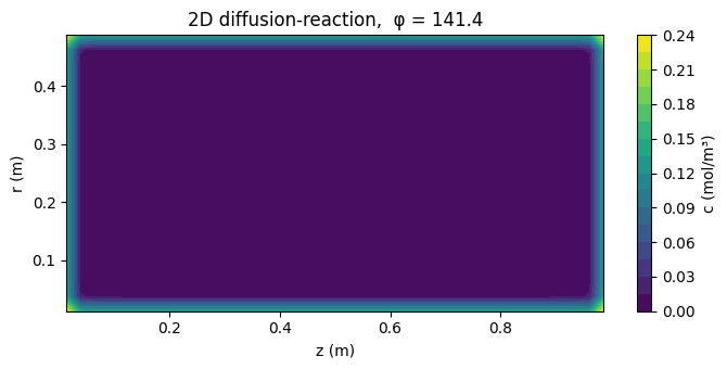
Example 1 — 2D Cartesian diffusion-reaction¶

Steady-state diffusion-reaction in a rectangular domain with Dirichlet BCs on all walls.

import numpy as np
import matplotlib.pyplot as plt
import scipy.sparse as sp
import scipy.sparse.linalg as spla

# Grid
Lz, Lr = 1.0, 0.5
Nz, Nr = 40, 20
dz, dr = Lz/Nz, Lr/Nr
z = (np.arange(Nz) + 0.5) * dz
r = (np.arange(Nr) + 0.5) * dr
D, k = 1e-4, 2.0
c_wall = 1.0

# 1D operators (face coordinates for pymrm)
z_f = np.linspace(0, Lz, Nz + 1)
r_f = np.linspace(0, Lr, Nr + 1)

# Assemble 2D Laplacian via Kronecker
# Interior operator (without ghost cells): use finite-difference tridiagonal
def laplacian_1d(N, h, D_coeff, bc='dirichlet'):
    main = -2*D_coeff/h**2 * np.ones(N)
    off = D_coeff/h**2
    A = sp.diags([off*np.ones(N-1), main, off*np.ones(N-1)], [-1,0,1], format='csr')
    rhs_bc = np.zeros(N)
    if bc == 'dirichlet':
        A[0, 0] -= off; A[-1, -1] -= off  # ghost-cell correction
        rhs_bc[0] = -2*off*c_wall; rhs_bc[-1] = -2*off*c_wall
    return A, rhs_bc

Az, rz = laplacian_1d(Nz, dz, D)
Ar, rr = laplacian_1d(Nr, dr, D)
Ir = sp.eye(Nr, format='csr')
Iz = sp.eye(Nz, format='csr')

L2D = sp.kron(Ir, Az) + sp.kron(Ar, Iz)
# RHS: BC contributions
rhs_z = np.tile(rz, Nr)   # repeated for each r row
rhs_r = np.repeat(rr, Nz) # repeated for each z column
rhs2D = rhs_z + rhs_r

# Reaction term: -k*c on diagonal
A2D = L2D - k * sp.eye(Nz*Nr)
c_flat = spla.spsolve(A2D, rhs2D)
C = c_flat.reshape(Nr, Nz)

ZZ, RR = np.meshgrid(z, r)
plt.figure(figsize=(7, 3.5))
plt.contourf(ZZ, RR, C, 20, cmap='viridis')
plt.colorbar(label='c (mol/m³)')
plt.xlabel('z (m)'); plt.ylabel('r (m)')
phi = np.sqrt(k/D)
plt.title(f'2D diffusion-reaction,  φ = {phi:.1f}')
plt.tight_layout(); plt.show()

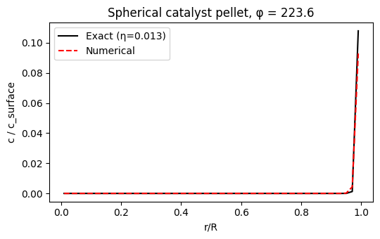
Example 2 — Cylindrical catalyst pellet¶

Spherical catalyst pellet with $\nu = 2$ : $\frac{d}{dr}\left(r^2 \frac{dc}{dr}\right) = \frac{r^2 k}{D} c$ . Use nu=2 in construct_div.

R_p = 1.0   # pellet radius [m] (normalised)
Np = 50
dr_p = R_p / Np
rp = (np.arange(Np) + 0.5) * dr_p
D_p, k_p = 1e-4, 5.0
phi_p = R_p * np.sqrt(k_p / D_p)

r_f_p = np.linspace(0, R_p, Np + 1)

# Build matrix: D_p * Dp @ diag(r²) @ Gp — use construct_div with nu=2
# Dirichlet at surface: c_ghost = 2*c_wall - c[-1]
c_surf = 1.0
off_p = D_p / dr_p**2
# Simplified: finite difference with cylindrical geometry
# d/dr(r^2 dc/dr)/r^2 = (1/dr^2)[c_{i+1} - 2c_i + c_{i-1}] + (1/r_i*dr)[c_{i+1}-c_{i-1}]
diag_p = -2*D_p/dr_p**2 - k_p
A_p = sp.diags([off_p*np.ones(Np-1), diag_p*np.ones(Np), off_p*np.ones(Np-1)],
               [-1, 0, 1], shape=(Np, Np), format='lil')
# Cylindrical correction: add (2/r_i) * D_p/dr_p * forward-backward diff
for i in range(1, Np-1):
    corr = D_p / (rp[i] * dr_p)
    A_p[i, i+1] += corr
    A_p[i, i-1] -= corr
# Symmetry BC at r=0: zero flux (Neumann)
A_p[0, 1] += off_p  # ghost = c[0] (reflection)
A_p = sp.csr_matrix(A_p)
rhs_p = np.zeros(Np)
rhs_p[-1] -= (off_p + D_p/(rp[-1]*dr_p)) * 2 * c_surf

c_p = spla.spsolve(A_p, rhs_p)

# Analytical: c = c_s * sinh(phi_p * r/R_p) / (r/R_p * sinh(phi_p))
c_anal_p = c_surf * np.sinh(phi_p * rp/R_p) / ((rp/R_p) * np.sinh(phi_p))
eta_exact = 3*(phi_p/np.tanh(phi_p) - 1)/phi_p**2

plt.figure(figsize=(5.5, 3.5))
plt.plot(rp/R_p, c_anal_p, 'k-', label=f'Exact (η={eta_exact:.3f})')
plt.plot(rp/R_p, c_p, 'r--', label='Numerical')
plt.xlabel('r/R'); plt.ylabel('c / c_surface')
plt.title(f'Spherical catalyst pellet, φ = {phi_p:.1f}')
plt.legend(); plt.tight_layout(); plt.show()

Summary¶

Kronecker product $\mathbf{I}_r \otimes \mathbf{L}_z + \mathbf{L}_r \otimes \mathbf{I}_z$ assembles the 2D Laplacian from 1D blocks
Array shape convention (Nz, Nr, Nc) stores all components at once; reshape to (Nz*Nr, Nc) for linear solvers
nu=1 (cylindrical) and nu=2 (spherical) in construct_div account for geometry
The symmetry boundary at $r=0$ requires a Neumann (zero-flux) condition
Effectiveness factor $\eta = \tanh(\phi)/\phi$ for slab, $3(\phi\coth\phi-1)/\phi^2$ for sphere