L4: Dispersion and Mass Transfer - Multiphase Reactor Modeling using PyMRM

Packed beds and multiphase reactors exhibit axial dispersion (back-mixing) and interphase mass transfer that profoundly affect conversion. This notebook presents the axial dispersion model, the Edwards-Richardson and Wakao-Funazkri correlations, and shows how to implement coupled fluid-particle models in pymrm using block-structured sparse matrices.

Governing equations¶

Axial dispersion model (fluid phase):

\varepsilon \frac{\partial c_f}{\partial t} + v \frac{\partial c_f}{\partial z} = \varepsilon D_{ax}\frac{\partial^2 c_f}{\partial z^2} - k_L a (c_f - c_s) + \varepsilon R_f

(1)

Particle phase (pseudo-steady):

k_L a (c_f - c_s) = (1-\varepsilon) R_s(c_s)

(2)

Edwards & Richardson axial dispersion correlation (packed bed):

\frac{D_{ax}}{v\,d_p} = \frac{0.73\,\varepsilon}{\varepsilon + 0.5/(Re\,Sc)} + \frac{0.5}{1 + 9.7\varepsilon/(Re\,Sc)}

(3)

Wakao & Funazkri mass-transfer correlation:

Sh = 2 + 1.1\,Re^{0.6}\,Sc^{1/3}

(4)

PyMRM building blocks¶

Function	Role
`construct_grad`, `construct_div`	Diffusion and divergence operators
`construct_convflux_upwind`	First-order upwind convective flux
`interp_cntr_to_stagg_tvd`	TVD convective flux
`scipy.sparse.block_diag`	Assemble multi-phase block system
`stencil_block_diagonals`	Extract/build block-tridiagonal structure

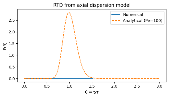
Example 1 — RTD from axial dispersion model¶

Compute the residence-time distribution (RTD) for a pulse input and compare the dispersion number $D_{ax}/vL$ with the Bodenstein number $Bo = vL/D_{ax}$ .

import numpy as np
import matplotlib.pyplot as plt
import scipy.sparse as sp
import scipy.sparse.linalg as spla
from pymrm import construct_grad, construct_div, construct_convflux_upwind

# Parameters
L, N = 1.0, 200
v = 0.1     # [m/s]
Dax = 1e-3  # [m²/s]
tau = L / v
Pe = v * L / Dax
dz = L / N
z = (np.arange(N) + 0.5) * dz
dt = 0.5 * dz / v   # CFL-limited
t_end = 3 * tau

x_f = np.linspace(0, L, N + 1)
x_c = 0.5 * (x_f[:-1] + x_f[1:])

# Pulse injection at t=0: Dirac approximated as top-hat
c = np.zeros(N)
c[0] = 1.0 / dz   # unit pulse

# BCs: zero flux at inlet (after pulse), zero gradient at outlet
bc_pulse = (
    {"a": 0, "b": 1, "d": 0.0},   # Dirichlet c=0 at inlet (after pulse)
    {"a": 1, "b": 0, "d": 0.0},   # Neumann dc/dz=0 at outlet
)
grad_mat, grad_bc = construct_grad(N, x_f, x_c, bc=bc_pulse)
div_mat = construct_div(N, x_f)
conv_mat, conv_bc = construct_convflux_upwind(N, x_f, x_c, bc=bc_pulse, v=v)

# Explicit time stepping
t = 0.0
c_out = []
t_out = []
while t < t_end:
    diff_flux = -Dax * (grad_mat @ c.reshape(-1, 1) + grad_bc)
    conv_flux = conv_mat @ c.reshape(-1, 1) + conv_bc
    total_flux = conv_flux + diff_flux
    dc = div_mat @ total_flux
    c += dt * dc.ravel()
    c = np.maximum(c, 0)  # positivity
    c_out.append(c[-1])
    t_out.append(t)
    t += dt

t_out = np.array(t_out)
c_out = np.array(c_out)
theta = t_out / tau

# Analytical RTD for open-open vessel
from scipy.stats import norm
c_anal = np.sqrt(Pe / (4*np.pi*theta + 1e-10)) * np.exp(-Pe*(1-theta)**2/(4*theta+1e-10))
c_anal[0] = 0

plt.figure(figsize=(6, 3.5))
plt.plot(theta, c_out * tau, label='Numerical')
plt.plot(theta, c_anal / tau * tau, '--', label=f'Analytical (Pe={Pe:.0f})')
plt.xlabel('θ = t/τ'); plt.ylabel('E(θ)')
plt.title('RTD from axial dispersion model')
plt.legend(); plt.tight_layout(); plt.show()

Example 2 — Heterogeneous packed bed with external mass transfer¶

Fluid phase with convection + dispersion coupled to particle phase via $k_L a$ .

# Wakao-Funazkri parameters
eps = 0.4           # bed void fraction
dp = 3e-3           # particle diameter [m]
mu = 1e-3           # dynamic viscosity [Pa·s]
rho_f = 1000.0      # fluid density [kg/m³]
D_mol = 1e-9        # molecular diffusivity [m²/s]
v_sup = 1e-3        # superficial velocity [m/s]
v_int = v_sup / eps

Re = rho_f * v_sup * dp / mu
Sc = mu / (rho_f * D_mol)
Sh = 2 + 1.1 * Re**0.6 * Sc**(1/3)
kL = Sh * D_mol / dp
a_p = 6 * (1-eps) / dp   # specific surface area [m²/m³]
kLa = kL * a_p

# Axial dispersion (simplified Bo = 10)
Bo = 10.0
Dax2 = v_int * L / Bo

# Steady-state: fluid with convection+dispersion, particle with reaction
# -eps*Dax c'' + v c' + kLa(c - c_s) = 0  (fluid)
# kLa(c_f - c_s) = (1-eps)*k*c_s           (particle, 1st order)
k_p = 1e-2   # particle reaction rate [1/s]
alpha = (1-eps) * k_p / kLa
c_s = lambda cf: cf / (1 + alpha)

# Solve fluid equation with effective sink
dz2 = L / N
off2 = eps * Dax2 / dz2**2
keff = kLa * alpha / (1 + alpha)
diag_v = np.full(N, v_int/dz2 + 2*off2 + kLa*alpha/(1+alpha))
# Build tridiagonal system
A3 = sp.diags([-off2 - v_int/dz2, diag_v, -off2],
              [-1, 0, 1], shape=(N, N), format='csr')
rhs3 = np.zeros(N)
c_in = 1.0
rhs3[0] += (off2 + v_int/dz2) * c_in
cf = spla.spsolve(A3, rhs3)
cs = c_s(cf)
z2 = (np.arange(N) + 0.5) * dz2

plt.figure(figsize=(6, 3.5))
plt.plot(z2, cf, label='Fluid phase c_f')
plt.plot(z2, cs, '--', label='Particle surface c_s')
plt.xlabel('z (m)'); plt.ylabel('c / c_in')
plt.title(f'Heterogeneous bed: Sh={Sh:.1f}, kLa={kLa:.3f} s⁻¹')
plt.legend(); plt.tight_layout(); plt.show()
print(f'Re={Re:.2f}, Sc={Sc:.0f}, Sh={Sh:.2f}, kL={kL:.2e} m/s')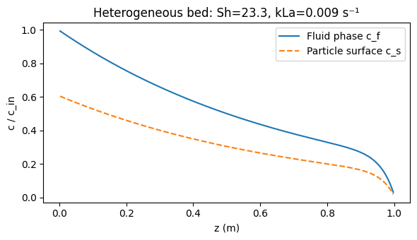

Re=3.00, Sc=1000, Sh=23.27, kL=7.76e-06 m/s

Summary¶

Bodenstein number $Bo = vL/D_{ax}$ characterises back-mixing: $Bo \to \infty$ = plug flow, $Bo \to 0$ = CSTR
Wakao & Funazkri: $Sh = 2 + 1.1\,Re^{0.6}\,Sc^{1/3}$ — widely used for packed beds
Edwards & Richardson: accounts for both molecular and mechanical dispersion
In a heterogeneous model the ratio $k_p/k_L a$ controls whether reaction or mass transfer limits
Block-diagonal sparse structure enables efficient coupled multi-phase solvers