A 2D Bubble Column Model - Multiphase Reactor Modeling using PyMRM

In a bubble column, the gas hold-up is larger in the middle. Rising bubbles induce a circulation pattern, dragging along the liquid in the middle, which circulates downward at the wall. We will model this by using radial profiles of hold-up and velocities. In most of the column, these profiles are constant along the height. However, at the bottom and top of the column, the flow will also be radially directed. These end zones will be modeled as ideally mixed, as indicated in the figure below.

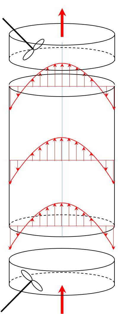
Schematic representation of the bubble-column model with ideally mixed end zones.

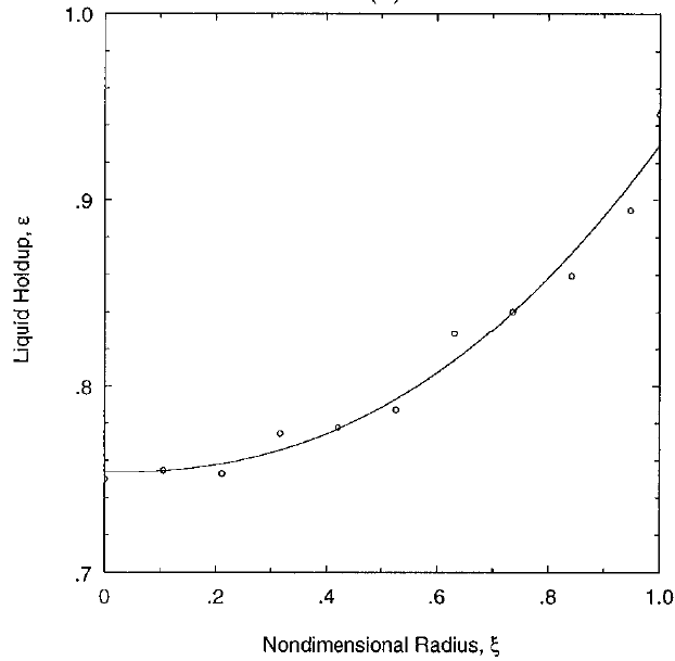
Radial profile of gas hold-up.

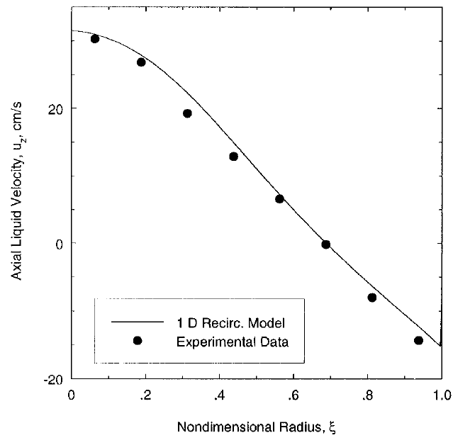
Radial profile of liquid velocity.

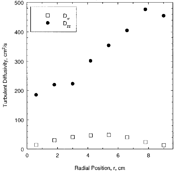
Radial profile of turbulent diffusivity.

The profiles plotted on the right are measured by means of radioactive particle tracking and taken from Degaleesan et al. (Ind. Eng. Chem. Res. 1997, 36, 4670-4680). The column diameter is $19~\mathrm{cm}$ , and the height is $190~\mathrm{cm}$ . The flow is in the churn turbulent regime.

From the experimental data plotted in the graphs above, we approximate:

\begin{align*} \varepsilon_{G}(r) &= 0.25 - 0.18 \frac{r}{R}, \quad \varepsilon_{L} = 1 - \varepsilon_{G}, \\ v_{L}(r) &= v_{L,0} \left( 1 - \frac{r}{0.7 R} \right), \\ D_{ax} &= 200~\mathrm{cm^{2}~s^{-1}} + \left( 300~\mathrm{cm^{2}~s^{-1}} \right) \frac{r}{R}, \\ D_{rad} &= 40~\mathrm{cm^{2}~s^{-1}}. \end{align*}

(1)

We assume that there is a difference $\Delta v_{GL}$ between the gas velocity and liquid velocity, independent of $y$ , such that:

v_{G}(r) = v_{L}(r) + \Delta v_{GL}.

(2)

The superficial velocity of the liquid equals $U_{L} = 1~\mathrm{cm~s^{-1}}$ , and for the gas: $U_{G} = 10~\mathrm{cm~s^{-1}}$ .

The total height of $190~\mathrm{cm}$ will be divided into three parts: a bottom section of $19~\mathrm{cm}$ , a middle section of $152~\mathrm{cm}$ , and a top section of $19~\mathrm{cm}$ . The middle section is modeled by means of the convection-diffusion-reaction equation:

\begin{align*} \frac{\partial}{\partial t} \left( \varepsilon_{L} c_{L} \right) + \frac{\partial}{\partial x} \left( \varepsilon_{L} v_{L} c_{L} - \varepsilon_{L} D_{ax} \frac{\partial c_{L}}{\partial x} \right) - \frac{1}{r} \frac{\partial}{\partial r} \left( r \left[ \varepsilon_{L} D_{rad} \frac{\partial c_{L}}{\partial r} \right] \right) &= k_{L} a \left( c_{L}^{*} - c_{L} \right) + \varepsilon_{L} R_{L}, \\ \frac{\partial}{\partial t} \left( \varepsilon_{G} c_{G} \right) + \frac{\partial}{\partial x} \left( \varepsilon_{G} v_{G} c_{G} - \varepsilon_{G} D_{ax} \frac{\partial c_{G}}{\partial x} \right) - \frac{1}{r} \frac{\partial}{\partial r} \left( r \left[ \varepsilon_{G} D_{rad} \frac{\partial c_{G}}{\partial r} \right] \right) &= -k_{L} a \left( c_{L}^{*} - c_{L} \right) + \varepsilon_{G} R_{G}. \end{align*}

(3)

Note that the turbulent diffusion coefficients for both liquid and gas are assumed to be identical. This is because small bubbles are dragged along with the liquid.

The top and bottom sections are modeled as ideally mixed. It is advised to model this by using artificially large axial and radial turbulent diffusion coefficients $D_{ax}$ and $D_{rad}$ in these sections. Also, ensure that the inflow in the bottom section is actually inflow (i.e., has no negative velocities) and that at the top, there is only outflow.

Questions:

Compute the average hold-ups and determine the values of $v_{L,0}$ and $\Delta v_{GL}$ such that the prescribed superficial velocities are obeyed.
Implement the formulated model equations in Python for the case of insoluble species ( $k_{L} a = 0$ ).
Model a first-order reaction in the liquid phase. Hint: Because you consider first-order kinetics, the result will be independent of the inlet concentration. A simple choice is $c_{L,\mathrm{in}} = 1~\mathrm{mol~m^{-3}}$ . How do the results for a range of kinetic coefficients compare to the conversion in an ideal CSTR and in a plug flow reactor?
Model a first-order reaction in the gas phase (for a range of kinetic coefficients). How does it compare to the conversion in an ideal CSTR and in a plug flow reactor?
Play with the model. Implement a realistic value of $k_{L} a$ , a proper equilibrium relation between gas and liquid concentrations (i.e., $c_{L}^{*}(c_{G})$ ), and interesting kinetics.

Note that all numerical implementations should be consistent with the provided equations and parameter values.