try:
    import pymrm
except ImportError:
%pip install -q pymrmThe gel effect without a switch: Chiu, Carratt and Soong’s diffusion-controlled termination
sec:J
struct:S1
tier:T0
data:tier6
phase:liquid
Chiu, Carratt & Soong (1983) build the Trommsdorff-Norrish gel effect out of one unbranched constitutive equation - 1/k_t = 1/k_t0 + theta_t P/f(x) - and criticise earlier treatments for switching diffusion control on at a prescribed critical conversion ‘in a somewhat ad hoc fashion’. THEIR COMPARISONS WITH EXPERIMENT LIVE ONLY IN FIGURES 3-9 (Marten & Hamielec’s data), SO THAT HALF OF THE CASE IS OUT OF SCOPE and nothing here is digitised; what the paper prints in numerals is two tables and six stated results, and this page tests those. THE HEADLINE IS THE PAPER’S OWN GRAPHICAL ONSET CONSTRUCTION, reconstructed from the sentence that defines it and computed rather than read: extrapolating the sloped region of log k_t back to its initial value gives 0.25516, 0.34838 and 0.44034 against the printed 0.26, 0.35 and 0.45, the largest miss 0.00966 in conversion, and the trend with temperature reproduced. THOSE ARE THE HIGHER INITIATOR LOADING, I_0 = 0.0258 mol/L, AND THE PAGE SAYS SO: the paper quotes one onset per temperature while Figures 10-12 plot both loadings, and the same construction on the other curve of the same figures misses by up to 0.03126. WHAT LIMITS THE NUMBER IS THE SENTENCE, NOT THE ARITHMETIC: seven defensible readings of the construction spread the answer by 0.09009, 9.33 times the largest miss, while the resampling grid moves it by 1.311e-05 relative and a completely independent integration - the six ODEs re-parametrised by conversion, different solver family - reproduces it to below 1e-10 relative. TWO OF THE PAPER’S OWN CORRELATIONS ARE RECOMPUTED FROM ITS OWN TABLE II: the Arrhenius activation energies of Figure 13 come out 34.908161 and 34.516600 kcal/mol against the printed 34 (+2.67 % and +1.52 %) and 27.771564 against the printed 28 (-0.82 %); and Figure 15’s claim that ‘all three points fall on the same straight line’ holds to 8.819e-04 relative, against 1.535e-02 for the same three points fitted linearly in T instead - 17.4057x worse at the printed T_gp, and not a nested submodel, so the direction is evidence. WHAT THAT COMPARISON ESTABLISHES IS CONCAVITY IN T AND NOT THE QUADRATIC FORM: the gain is 3.6124x and 3.5347x at the two ends of the T_gp interval the same three cells admit and diverges inside it, and two other non-nested two-parameter regressors beat linear-in-T as well (5.5926x and 3.2607x), so what all of them are reading is the second difference of A, -0.007000. THE MODEL’S OWN FRAMING IS TESTED RATHER THAN RESTATED. ‘Only a small number of adjustable parameters’ means four named parameters and THIRTEEN fitted numbers over six conditions; the paper’s own Figures 13 and 15 compress those thirteen to eight, but only to 18.8281 % on theta_t, which moves the onset conversion by 0.01633 - 1.691 times the distance by which this page’s reconstruction misses the printed onsets, so the compression is lossy at the resolution of the paper’s own results. And the ‘ad hoc’ criticism survives a quantitative test: eq. 31 and 32 carry no branch at all, the nearest thing to an onset knob (theta_t) moves the onset by only -0.21735 per decade against 1.0 per unit for a prescribed critical conversion, and the counterfactual - the same model switched on at x_c = 0.3 - is concave DOWN over its whole pre-switch portion and jumps 0.760194 of a decade in log k_t at the switch, which is exactly the argument the paper makes on book p. 353. FIVE INTERNAL IDENTITIES ARE PROVED RATHER THAN ASSERTED: eq. 24 and eq. 26 are re-derived symbolically from eq. 21 and come out exactly zero, eq. 22’s ‘r_D >> r_m’ is shown to cost EXACTLY r_m/r_D - symbolically, and then a second time through the flux a pymrm spherical-shell BVP actually computes, which lands on r_m/r_D to 1.858e-05 over five ratios and converges onto it at observed order 1.8953 - and the moment equations 12-17 reproduce the chain-length equations 4a, 4b and 5 summed over a seeded finite population to below 1e-14 relative, including the k_tc terms, which Table I sets to zero and which therefore no condition the paper reports ever exercises. Three printed features are reported and not repaired: Figure 3’s legend prints 0.01584 where five other printings give 0.01548, Table I gives the first-order k_d the units L/min, and book p. 353 reads ‘The presence model’ [sic].
The gel effect without a switch
Catalog ID: J5.3 · Structures: S1 · Tier: T0
Background
The source is on disk and all ten of its pages were read at the file’s native resolution:
Chiu, W. Y., Carratt, G. M. and Soong, D. S., A Computer Model for the Gel Effect in Free-Radical Polymerization, Macromolecules 16(3), 348-357 (1983), doi:
10.1021/ma00237a002.
Identity was confirmed from the document’s own title block on a 300 ppi render - the title, the by-line “Wen Yen Chiu, Gregory M. Carratt, and David S. Soong”, the department line “Department of Chemical Engineering, University of California, Berkeley, California 94720”, “Received July 1, 1982” and the running head “Macromolecules 1983, 16, 348-357”. pdfimages -list reports every page as CCITT-G4 bilevel at 300x300 ppi, so 300 ppi is native and rendering higher would be interpolation.
The file straddles three articles, at both ends
PDF page 1 opens with the References and Notes of the PRECEDING article - a Zambelli stereochemistry paper, references 1-28 - and Chiu et al. begin below them, halfway down the page. PDF page 10 opens the NEXT article: the running head there reads “Macromolecules 1983, 16, 357-359” and the title is “Radical Reactions of Highly Polar Molecules. Hydrocarbons as Chain-Transfer Agents in Fluoro Olefin Telomerizations” by Leonard O. Moore. That article has a Table I of its own, about the chain length of normal alkanes, so a search for “Table” over the whole file conflates two papers.
Every numeral used on this page was therefore located twice: first on a page whose running head reads “Gel Effect in Free-Radical Polymerization” or “Chiu, Carratt, and Soong”, and then on a crop of that page enlarged to digit scale. Chiu’s own tables are Table I on book p. 352 and Table II on book p. 353, both inside PDF pages 1-9.
What the paper prints in numerals, and what it does not
| where | what | |
|---|---|---|
| Table I | book p. 352 (PDF 5) | “Numerical Values of Parameters Used in Model Calculation” - eight lines of constants, attributed by its own heading to refs 6 and 7 |
| Table II | book p. 353 (PDF 6) | “Model Parameters Used in Fitting Experimental Data” - six rows of the four fitted parameters |
| running text | book pp. 354-356 | six stated numerical results about the model’s own output |
| Figures 3-9 | book pp. 352-354 | the experimental data, Marten & Hamielec’s, plotted against the model’s curves |
The comparison with experiment lives only in the figures, so that half of the case is out of scope and no curve is digitised. The paper reports no measurement of its own: reference 7, Marten, F. L. & Hamielec, A. E., ACS Symp. Ser. 1979, No. 104, 43, supplies the conversion and molecular-weight data, and none of it is tabulated here. The page therefore establishes nothing about this model’s empirical adequacy, and says so wherever that matters.
What is left is worth more than it sounds. Table II’s parameters were fitted to those figures - the table says so in its title - so anything computed from them and compared with the paper is a consistency check on the authors’ own fit and on this page’s transcription, never a validation against nature. But the paper also states six numerical results about its own output, prints two correlations that its own tables must satisfy, and makes two structural claims about the model that are checkable without any data at all. Those are what this page tests.
What this page finds
The paper’s own onset construction, reconstructed and computed. Book p. 354 defines the onset of the gel effect as the intersection of a line extrapolated from “the sloped region” of the log k_t curve with “the initial value”, and states the answers: “This intersection occurs around a conversion level of 0.26 for 50 °C, 0.35 for 70 °C, and 0.45 for 90 °C.” Reconstructed as a least-squares line over the decades L_0-2 to L_0-4 and extrapolated to L_0 = log10 k_t^0, the model gives 0.25516, 0.34838 and 0.44034 - all three low, by 0.00484, 0.00162 and 0.00966 at worst, with the increase with temperature reproduced.
Those are at I_0 = 0.0258 mol/L, and the choice is stated rather than implied. The paper quotes one onset per temperature; Figures 10-12 plot both loadings and the sentence names neither. 0.0258 is the loading listed first in all three legends and the one Figures 16-18 plot, and that is the whole basis for the choice - the paper gives no other. The same construction on the 0.01548 curve of the same figures misses by up to 0.03126, 3.24 times the headline miss, and the page prints both columns beside each other.
The construction is a graphical one described in words, so its definitional band matters more than its precision. Seven defensible readings - six of “the sloped region” (four decade windows and two tangents) and one of “the initial value” - spread the answer by up to 0.09009, 9.33 times the largest miss. That band is a spread over seven readings and not a bound over every reading of the sentence: the most literal reading of all, the tangent at the steepest point of the descent, gives 0.44783, 0.47680 and 0.51866 and lies outside it. It is excluded for a measured reason, printed with the number - its tangent point sits at x = 0.86, the right edge of this page’s window, at all six conditions, so that reading is set by where the curve is truncated rather than by the curve.
One reading is kept out and the exclusion is measured, so the same measurement has to be applied to every reading the band keeps in. The 4-6-decade window is the widest-swinging of the seven - 0.29957, 0.41999 and 0.49516 - and leaving it out was therefore the flattering choice; the notebook applies the truncation test to it and it passes, its fit mask ending inside x = 0.86 at four of the six conditions, including the condition at which the reported band is widest. It is in the band because the page cannot exclude it on a measurement, which is the only ground on which anything here is excluded.
Two arithmetic floors, neither of which is what limits the number. The resampling grid moves the onsets by 1.311e-05 relative - the sixth decimal of every onset here is grid noise, which is why five are quoted - and a completely independent integration reproduces them to below 1e-10 relative, round-off whose exact digits differ from machine to machine. That second number prices the attractor, not the integration: lambda_0(x) sits on a strongly attracting manifold, so two parametrisations of the same equations land on the same log k_t(x) however they got there. Both floors are orders of magnitude inside the definitional band, and the page says so rather than quoting the digits the fit returns.
Two of the paper’s own correlations, recomputed from its own Table II. Figure 13’s Arrhenius plots give 34.908161 and 34.516600 kcal/mol for theta_t at the two initiator loadings against the printed 34 (+2.67 % and +1.52 %, mean 34.712380, +2.10 %), and 27.771564 for theta_p against the printed 28 (-0.82 %). Figure 15’s “All three points fall on the same straight line” holds to 8.819e-04 relative - against 1.535e-02 for the same three points fitted linearly in T instead, 17.4057x worse, and the two forms are not nested, so the direction of that ratio is evidence and not algebra. The T_gp that would make the three A values exactly collinear is 111.42857 °C against Table I’s printed 114, but the printed rounding of A alone admits [102.2222, 128.0000] °C, so the three cells cannot distinguish them and the page reports the interval rather than the point. The exponent the same three cells pick out at the printed T_gp is 2.0659.
And the 17.4057x is the gain at one admissible T_gp, not a property of the data - so what the comparison establishes is concavity in T, not the Fujita/glass-transition form. The same gain is 3.6124x and 3.5347x at the two ends of that interval and diverges at 111.42857 °C, where the three points are exactly collinear by construction. And the quadratic is not singled out: A against 1/T beats linear-in-T by 5.5926x and A against (T - 130)^2 by 3.2607x, both two-parameter, neither nested. With three points and one residual degree of freedom, what every one of them is reading is that A is concave in T - the three values are equally spaced in T and their second difference is -0.007000 - which linear-in-T cannot represent and any sufficiently curved regressor can. The page claims the concavity.
“Only a small number of adjustable parameters” - counted, then exercised. The paper names four (theta_t, theta_p, A, B); Table II fits 13 distinct numbers across 6 conditions, 2.1667 per condition. Its own Figures 13 and 15 compress those 13 to 8 - and the compression reproduces A to 0.0882 %, theta_p to 8.3695 % but theta_t only to 18.8281 %, which moves the onset conversion by 0.01633, 1.691 times the distance by which this page’s reconstruction misses the printed onsets. So “Figures 13 and 15 provide an effective means to estimate all the model parameters” is true as a procedure and lossy as an identity, and the loss sits in theta_t.
“In a somewhat ad hoc fashion” - the criticism holds, and here is the measurement. Eq. 31 and 32 carry no branch: k_t and k_p are smooth in x everywhere, and the implementation contains no conditional except the one that builds the counterfactual. The nearest thing to an onset knob is theta_t, and it moves the onset by -0.21735 per decade; a prescribed critical conversion moves it by 1.0 per unit of itself, by construction, so it takes 4.601 decades of theta_t to buy one unit of onset. And the counterfactual settles the paper’s own argument on book p. 353: the same model switched on at x_c = 0.3 is concave down over 100 % of its pre-switch portion (largest d2x/dt2 there, -1.391e-06) and jumps 0.760194 of a decade in log k_t at the switch - both factors of that expression evaluated at x_c exactly, the radical concentration root-found on the dense solution rather than read off the nearest grid point - while the published model is concave up from x = 0.30643 to the sharp rise, with every onset inside that window; the smallest margin is 0.129. One qualification the paper does not make: the published model’s conversion curve is concave down below that lower bound - initiator depletion, before diffusion limitation takes over - so “concave upward preceding the sharp rise” is true of the region the paper means and not of the whole pre-gel curve.
The quasi-steady-state assumption, measured at all six conditions instead of one. Book p. 356: “The QSSA solution overestimates the radical concentration by more than a factor of 2.” At the condition Figures 16-18 plot - 50 °C, I_0 = 0.0258 - it is 3.5176x, and the conversion history nevertheless differs by at most 0.038611 in x, which is the paper’s “surprisingly consistent”. Across all six conditions the factor runs 1.4889 to 4.8466 and exceeds 2 at three of them and fails at three; it falls with temperature and rises as the initiator loading falls. The paper states it for the one condition it plots and claims no more, and this page measures the other five.
Five identities proved rather than asserted. Eq. 24 and eq. 26 are re-derived symbolically from eq. 21 with the paper’s own boundary conditions and come out exactly zero; eq. 22’s “Since r_D >> r_m” is shown to cost exactly r_m/r_D, symbolically and then a second time through the flux a pymrm spherical-shell BVP actually computes - 4 pi r^2 D dC/dr read off the solved profile, which lands on r_m/r_D to 1.858e-05 over five ratios at n = 6400 and converges onto it at observed order 1.8953; and the moment equations 12-17 reproduce eq. 4a, 4b and 5 summed over a seeded finite population to a relative residual below 1e-14, both with k_tc = 0 and with a non-zero k_tc that no printed condition exercises.
And one thing the model does that the paper’s prose does not mention. “The limiting conversion at long times is lowest at 50 °C and gradually increases with the polymerization temperature” is reproduced as an ordering - 0.95535, 0.98173, 0.99289 at a stated rate threshold, smallest gap 0.011165 - but this model has no limiting conversion in the mathematical sense: as x -> 1 the Fujita-Doolittle factor returns to 1, 1/k_p -> 1/k_p^0 + theta_p lambda_0 stays finite, and dx/dt vanishes only through (1-x). Integrated far enough every condition creeps on, to 0.97897, 0.99850 and 0.99998 at the horizons used here and still rising. The plateau in Figures 3-5 is where the curve stops being drawn.
The published model
Mechanism and balances (eq. 1-9). Initiation I -> 2R, R + M -> P_1; propagation P_n + M -> P_{n+1}; termination by combination P_n + P_m -> M_{n+m} (rate constant k_tc) and by disproportionation P_n + P_m -> M_n + M_m (k_td), with k_t = k_tc + k_td. The species balances are written per unit volume of a batch whose volume contracts with conversion, V = V_0 (1 + eps x) with eps = (d_m - d_p)/d_p (eq. 6), and the chain-length distributions are reduced by the method of moments, lambda_k = sum n^k P_n for the growing radicals and mu_k = sum n^k M_n for the dead polymer (eq. 8-9).
The eight equations this page integrates (eq. 10-18). In the paper’s own form, with the quasi-steady-state assumption applied to the PRIMARY radical R only (eq. 18, k_i R M = 2 f k_d I) and not to the polymer radicals:
dI/dt      = -k_d I - [eps I/(1+eps x)] lambda_0 (1-x) k_p                (10)
dx/dt      =  k_p (1-x) lambda_0                                          (11)
dlambda_0/dt = -[eps lambda_0/(1+eps x)] lambda_0 (1-x) k_p
               + 2 f k_d I - k_t lambda_0^2                               (12)
dlambda_1/dt = ... + 2 f k_d I - k_t lambda_0 lambda_1
               + k_p lambda_0 M_0 (1-x)/(1+eps x)                         (13)
dlambda_2/dt = ... + 2 f k_d I - k_t lambda_0 lambda_2
               + k_p M_0 (1-x)/(1+eps x) (2 lambda_1 + lambda_0)          (14)
dmu_0/dt   = ... + k_td lambda_0^2 + (1/2) k_tc lambda_0^2                (15)
dmu_1/dt   = ... + k_td lambda_0 lambda_1 + k_tc lambda_0 lambda_1        (16)
dmu_2/dt   = ... + k_td lambda_0 lambda_2
               + k_tc (lambda_2 lambda_0 + lambda_1^2)                    (17)
with I = I_0 and x = lambda_k = mu_k = 0 at t = 0, and average molecular weights from eq. 19 and 20, which keep the growing-radical moments: Mn = (mu_1 + lambda_1)/(mu_0 + lambda_0), Mw = (mu_2 + lambda_2)/(mu_1 + lambda_1).
The constitutive part, which is what the paper is about (eq. 21-32). A radical pair terminates only after one radical migrates to within r_m of the other. Between r_m and a far radius r_D the migration is a steady spherical diffusion problem,
4 pi r^2 D dC/dr = K, C(r_m) = C_m, C(r_D) = C_b (21)whose first integral, with r_D >> r_m, is eq. 22, and which balanced against the consumption inside r_m (eq. 23) gives eq. 24, eq. 25 and finally
1/k_t = 1/k_t^0 + r_m^2 C_b/(3 D) (26)a series of a reaction resistance and a mass-transfer resistance, with no switch anywhere. Splitting D into a front factor and a conversion-dependent part, D = D_0 f(x), and calling theta_t = r_m^2/(3 D_0) gives eq. 27; the same argument applied to monomer diffusion to the radical end gives eq. 28 for k_p; and the Fujita-Doolittle free-volume form (eq. 29) with the monomer volume fraction of eq. 30 closes both:
1/k_t = 1/k_t^0(T) + theta_t(T, I_0) P / exp[2.3 phi_m/(A(T) + B phi_m)]  (31)
1/k_p = 1/k_p^0(T) + theta_p(T)      P / exp[2.3 phi_m/(A(T) + B phi_m)]  (32)
where P = lambda_0 and phi_m = (1-x)/(1+eps x). Eq. 31 and 32 are the whole model of the gel and glass effects, and they carry no branch, no critical conversion and no conditional of any kind. That is the paper’s central claim and this page checks it as a claim, not as a slogan.
The two claims of the paper’s own framing, which this page tests
On parameter count, book p. 349:
“In order for the model to be useful in process simulation and design calculation, it must quantitatively predict experimental data obtained under well-controlled conditions while requiring only a small number of adjustable parameters.”
On the alternative treatments, book p. 351:
“The second difficulty with the conventional modeling approach is associated with the somewhat artificial introduction of a sudden onset of diffusion influence on
k_t. In other words,k_tremains constant until either the concentration or some sort of combination of concentration and molecular weight (of the dead polymer) reaches a prescribed critical value, whereuponk_tbecomes proportional to the diffusion coefficient. This creates an adjustable parameter to determine when the gel effect computation is switched on - in a somewhat ad hoc fashion.”
Both are checkable. The first by counting the fitted numbers and then exercising the paper’s own compression of them; the second by asking what in this model plays the part a critical conversion plays in the others, and measuring how directly it sets the answer.
Parameters and assumptions
Everything numerical comes from the two tables, parsed out of CSVs rather than retyped in a cell. Table I is not this paper’s measurement: its own heading carries the reference marks 6,7, so the constants are Schmidt & Ray’s and Marten & Hamielec’s. Neither of those is on disk, so nothing here is traced past this table and both are recorded as origins not consulted.
One input is a reconstruction and it is labelled one everywhere. The moment equations 13, 14, 16 and 17 need the initial monomer concentration M_0 = d_m/MW, and the molar mass of methyl methacrylate is printed nowhere in the paper. The paper prints the monomer density line and, on book p. 356, the Registry No. 80-62-6; MW = 100.117 g/mol follows from C5H8O2 and standard atomic weights. It cannot touch any headline on this page, and the notebook demonstrates that rather than asserting it: doubling MW moves the conversion history by less than 1e-10 and lambda_0 by less than 1e-9 relative - both solver noise - and mu_1 by 0.499939, exactly the factor it should. Eq. 10, 11 and 12 contain no M_0 at all, so x(t), lambda_0, k_t, k_p and every onset number are independent of it; only the molecular weights are not.
Two printed features of Table I are reported and not repaired.
k_dis printed with the unitsL/minalthough eq. 1,(1/V) d(IV)/dt = -k_d I, makes it a first-order constant whose units are1/min. The CSV carries the printed string; the page uses1/minand labels that an inference from eq. 1.k_tc = 0, “[termination by disproportionation only]”. That is the authors’ choice and it makes part of their own published model inert: everyk_tcterm in eq. 5, 15, 16 and 17 is unexercised by any condition the paper reports. The paper states the consequence itself on book p. 352 - “Note that termination by recombination is ignored in the calculation, so the molecular weight predictions will be underestimated” - and this page exercises those terms once, in the moment identity, with ak_tcthat is printed nowhere.
And one arithmetic check settles the transcription of Table I. Evaluated at the three temperatures, the printed constants give log10 k_t^0 = 9.2952, 9.3229, 9.3475 and log10 k_p^0 = 4.5256, 4.6972, 4.8499, and Figures 10, 11 and 12 plot exactly those two quantities against conversion on an axis labelled 0 to 12, with the plateaux at about 9.3 and about 4.5. That is a corroboration of the transcription and not a data source: no value read off any figure enters a CSV, a fit or a metric anywhere on this page.
The data
Three CSVs, all transcription of printed numerals, provenance tier 6 - the paper’s own tabulated values and stated results, nothing digitised:
| dataset | rows | what |
|---|---|---|
chiu1983-table1-rate-constants |
8 | Table I, parsed into kind/a/b plus the line as printed |
chiu1983-table2-model-parameters |
6 | Table II, (T, I_0, theta_t, theta_p, A, B) |
chiu1983-stated-results |
6 | the six numerical results the running text and Figure 13’s caption state, each with the sentence it was read from |
FIT, NOT TEST, and the page says so at every use. Table II’s title is “Model Parameters Used in Fitting Experimental Data” and Figure 13’s caption repeats it - “Model parameters theta_t and theta_p chosen for the best fit of experimental data”. So theta_t, theta_p and A were chosen to make the model match Figures 3-9, and every number this page computes from them is a consistency check on that fit and on this transcription. The stated results are the model’s own output, so reproducing them is reproduction, not validation. Nothing on this page is a comparison with a measurement, because every measurement in this paper is a marker on a figure.
A printed discrepancy in the initiator loading, reported and not repaired. Table II’s lower loading is 0.01548 mol/L, and so are the legends of Figures 4, 5 and 8 and the captions of Figures 6 and 8. The legend of Figure 3 prints 0.01584 - the last two digits transposed - read at 3x on the 300 ppi bilevel image, where the glyphs are unambiguous. Five printings against one make 0.01548 the value the CSV carries, and the odd one out is recorded rather than corrected. Nothing on the page depends on which is right: Table II is what the model is run from.
One typographical defect elsewhere, quoted verbatim. Book p. 353 reads “The presence model, however, successfully correlates Mw and Mn at various conversion levels with temperature and initiator loading” [sic] - presence for present. Reported, not repaired, and nothing depends on it.
import json
import re
import sys
from pathlib import Path

import matplotlib.pyplot as plt
import numpy as np
import pandas as pd
from scipy.integrate import solve_ivp
from scipy.interpolate import CubicSpline
from scipy.optimize import brentq
from scipy.sparse.linalg import spsolve

from pymrm import NumJac, construct_div, construct_grad, newton

# gallery_utils: from the checkout when there is one, from raw GitHub on Colab
if "google.colab" in sys.modules:
    import urllib.request
    urllib.request.urlretrieve(
        "https://raw.githubusercontent.com/computational-chemical-engineering/"
        "pymrm-gallery/main/shared/gallery_utils.py", "gallery_utils.py")
else:
    for _p in (Path.cwd(), *Path.cwd().parents):
        if (_p / "shared" / "gallery_utils.py").is_file():
            sys.path.insert(0, str(_p / "shared"))
            break
from gallery_utils import Claims, cite_data, load_data, load_meta, parse_literal

PAGE = "J5.3-chiu-gel-effect"
plt.rcParams.update({"figure.dpi": 110, "font.size": 9.5})
# Okabe-Ito, assigned in fixed order and never cycled
C_BLUE, C_ORANGE, C_GREEN = "#0072B2", "#D55E00", "#009E73"
C_PURPLE, C_YELLOW, C_GREY = "#CC79A7", "#E69F00", "0.45"

# DETERMINISM: nothing on this page is stochastic.  No sampling, no bootstrap,
# no random initial guess and no continuation chain - every integration starts
# from the same t = 0 state, so no answer can depend on a sweep order.  The one
# pseudo-random object on the page is the test population of the moment-closure
# identity, and it is drawn from a SEEDED generator.
SEED = 19830348          # volume and first page of the article

T1 = load_data("chiu1983-table1-rate-constants.csv", page=PAGE)
T2 = load_data("chiu1983-table2-model-parameters.csv", page=PAGE)
TS = load_data("chiu1983-stated-results.csv", page=PAGE)
for _n in ("chiu1983-table1-rate-constants.csv",
           "chiu1983-table2-model-parameters.csv",
           "chiu1983-stated-results.csv"):
    print(cite_data(load_meta(_n, page=PAGE)))
print(f"\nTable I  : {len(T1)} printed lines")
print(f"Table II : {len(T2)} rows, {T2.polym_temp_C.nunique()} temperatures,"
      f" {T2.initiator_loading_mol_per_L.nunique()} initiator loadings")
print(f"stated   : {len(TS)} numerical results quoted in text or captions")
Chiu, W. Y.; Carratt, G. M.; Soong, D. S. (1983) — "A Computer Model for the Gel Effect in Free-Radical Polymerization", Macromolecules 16(3) 348-357 (1983), Department of Chemical Engineering, University of California, Berkeley, California 94720
— doi:10.1021/ma00237a002 — transcription
Chiu, W. Y.; Carratt, G. M.; Soong, D. S. (1983) — "A Computer Model for the Gel Effect in Free-Radical Polymerization", Macromolecules 16(3) 348-357 (1983)
— doi:10.1021/ma00237a002 — transcription
Chiu, W. Y.; Carratt, G. M.; Soong, D. S. (1983) — "A Computer Model for the Gel Effect in Free-Radical Polymerization", Macromolecules 16(3) 348-357 (1983)
— doi:10.1021/ma00237a002 — transcription
Table I : 8 printed lines
Table II : 6 rows, 3 temperatures, 2 initiator loadings
stated : 6 numerical results quoted in text or captions# ---- Table I, parsed from the CSV. No constant is retyped in a cell. -------
R_CAL = 1.987 # the gas constant Table I itself writes into k_t0
_t1 = T1.set_index("symbol")
def _row(sym):
r = _t1.loc[sym]
return str(r.kind), float(r.a), (np.nan if pd.isna(r.b) else float(r.b))
F_EFF = _row("f")[1]
KD_A, KD_B = _row("k_d")[1], _row("k_d")[2]
KT0_A, KT0_E = _row("k_t0")[1], _row("k_t0")[2]
KP0_A, KP0_E = _row("k_p0")[1], _row("k_p0")[2]
KTC = _row("k_tc")[1]
D_POLY = _row("d_p")[1]
DM_A, DM_B = _row("d_m")[1], _row("d_m")[2]
T_GP = _row("T_gp")[1]
def k_d(T):
"""1/min. Table I prints the units as L/min; eq. 1 makes it first order."""
return KD_A*np.exp(-KD_B/T)
def k_t0(T):
return KT0_A*np.exp(-KT0_E/(R_CAL*T))
def k_p0(T):
return KP0_A*np.exp(-KP0_E/(R_CAL*T))
def d_m(T):
return DM_A - DM_B*(T - 273.0) # 273, not 273.15, as printed
MW_MMA = 100.117 # RECONSTRUCTION - see the note below
print("Table I as parsed:")
for s in _t1.index:
k, a, b = _row(s)
print(f" {s:6s} {k:24s} a = {a:<12g} b = {'' if np.isnan(b) else b}")
print(f"\nat 50/70/90 degC:")
for TC in (50, 70, 90):
T = TC + 273.15
print(f" {TC} degC: k_d = {k_d(T):.6e} 1/min log10 k_t0 = {np.log10(k_t0(T)):.4f}"
f" log10 k_p0 = {np.log10(k_p0(T)):.4f} d_m = {d_m(T):.6f} g/cm3")Table I as parsed:
f constant a = 0.58 b =
k_d arrhenius_over_T a = 6.32e+16 b = 15430.0
k_t0 arrhenius_over_RT a = 5.88e+09 b = 701.0
k_p0 arrhenius_over_RT a = 2.95e+07 b = 4353.0
k_tc constant a = 0 b =
d_p constant a = 1.2 b =
d_m linear_in_T_minus_273 a = 0.973 b = 0.001164
T_gp constant a = 114 b =
at 50/70/90 degC:
50 degC: k_d = 1.158004e-04 1/min log10 k_t0 = 9.2952 log10 k_p0 = 4.5256 d_m = 0.914625 g/cm3
70 degC: k_d = 1.872131e-03 1/min log10 k_t0 = 9.3229 log10 k_p0 = 4.6972 d_m = 0.891345 g/cm3
90 degC: k_d = 2.227592e-02 1/min log10 k_t0 = 9.3475 log10 k_p0 = 4.8499 d_m = 0.868065 g/cm3PyMRM implementation
This is an S1 case - an ODE initial-value problem in time, no space - so what pymrm contributes is a solver and a Jacobian, not an operator stack. Two pieces of pymrm are used and both are exercised with a refinement study under Validation:
- A backward-Euler marcher on the eight fields built from
newtonandNumJac((1, 8)). The shape is(1, 8)and not(8,)deliberately: with a bare 1-D shape the last axis is read as space, the default stencil declares every cell coupled to every other, and the Jacobian comes out dense. Here that is 8x8 either way, but the shape is written the way that generalises. The eight fields are scaled before marching, becausenewtontests the infinity norm of the Newton update and these states span twenty orders of magnitude (lambda_0 ~ 1e-8 mol/Lagainstmu_2 ~ 1e8); one absolute tolerance means nothing across that range and everything in the scaled ones. - The paper’s own eq. 21 as a 1-D spherical BVP, with
construct_gradandconstruct_div(nu=2)on the shellr_m <= r <= r_Dand Dirichlet data at both ends. This is where pymrm buys something the paper does not have: eq. 22 drops the1/r_Dterm with the words “Sincer_D >> r_m”, and solving the shell problem prices that approximation exactly.
The physics itself is a plain Chiu class - the eight right-hand sides of eq. 10-17 and the two constitutive equations 31-32 - integrated with BDF for the reference solution, because the system is stiff by four orders of magnitude once the gel effect sets in. The class contains one if, and it is not in the model: it selects the counterfactual switched-on variant used to test the paper’s argument in Validation. The published model is the branch-free one.
# ---- the published model, eq. 10-18 with the constitutive eq. 31-32 --------
class Chiu:
    """One experimental condition of Table II.

    States, in the order the residual uses them:
        I, x, lam0, lam1, lam2, mu0, mu1, mu2
    eq. 10-17 verbatim; eq. 18 (the QSSA on the PRIMARY radical R) is already
    substituted, which is what turns k_i R M into 2 f k_d I.
    """

    FIELDS = ("I", "x", "lam0", "lam1", "lam2", "mu0", "mu1", "mu2")

    def __init__(self, T_C, I0, theta_t=None, theta_p=None, A=None, B=None,
                 ktc=None, ln10=2.3, switch_xc=None):
        r = T2[(T2.polym_temp_C == T_C)
               & np.isclose(T2.initiator_loading_mol_per_L, I0)]
        assert len(r) == 1, f"Table II has no unique row for {T_C} degC, {I0} mol/L"
        r = r.iloc[0]
        self.T_C, self.I0 = float(T_C), float(I0)
        self.T = self.T_C + 273.15
        self.theta_t = float(r.theta_t_min) if theta_t is None else theta_t
        self.theta_p = float(r.theta_p_min) if theta_p is None else theta_p
        self.A = float(r.A) if A is None else A
        self.B = float(r.B) if B is None else B
        self.ktc = KTC if ktc is None else ktc
        self.ln10 = ln10                  # the 2.3 eq. 31 prints, not ln(10)
        self.switch_xc = switch_xc        # None = the published model, no switch
        self.kd, self.kt0, self.kp0 = k_d(self.T), k_t0(self.T), k_p0(self.T)
        self.dm = d_m(self.T)
        self.eps = (self.dm - D_POLY)/D_POLY      # volume expansion factor
        self.M0 = self.dm*1000.0/MW_MMA           # needs the RECONSTRUCTED MW

    # ------------------------------------------------------ constitutive part
    def phi_m(self, x):
        """eq. 30: volume fraction of monomer."""
        return (1.0 - x)/(1.0 + self.eps*x)

    def fujita(self, x):
        """D/D_0 from eq. 29 as eq. 31/32 write it, exp[2.3 phi_m/(A+B phi_m)]."""
        pm = self.phi_m(x)
        return np.exp(self.ln10*pm/(self.A + self.B*pm))

    def kt_kp(self, x, P):
        """eq. 31 and 32.  NO BRANCH: one expression over the whole range."""
        g = self.fujita(x)
        if self.switch_xc is None:
            kt = 1.0/(1.0/self.kt0 + self.theta_t*P/g)
            kp = 1.0/(1.0/self.kp0 + self.theta_p*P/g)
            return kt, kp
        # the COUNTERFACTUAL the paper argues against: constant until x_c
        on = np.asarray(x) >= self.switch_xc
        kt = np.where(on, 1.0/(1.0/self.kt0 + self.theta_t*P/g), self.kt0)
        kp = np.where(on, 1.0/(1.0/self.kp0 + self.theta_p*P/g), self.kp0)
        return kt, kp

    # ------------------------------------------------------------ the ODE set
    def rhs(self, t, y):
        I, x, l0, l1, l2, m0, m1, m2 = y
        x = min(max(x, 0.0), 1.0 - 1e-12)
        kt, kp = self.kt_kp(x, l0)
        ktd = kt - self.ktc                   # k_t = k_tc + k_td, eq. 4b
        e, M0 = self.eps, self.M0
        dil = e*(1.0 - x)*kp*l0/(1.0 + e*x)   # (1/V) dV/dt
        M = M0*(1.0 - x)/(1.0 + e*x)          # eq. 7
        gen = 2.0*F_EFF*self.kd*I             # eq. 18 substituted
        return np.array([
            -self.kd*I - dil*I,                                      # eq. 10
            kp*(1.0 - x)*l0,                                         # eq. 11
            -dil*l0 + gen - kt*l0*l0,                                # eq. 12
            -dil*l1 + gen - kt*l0*l1 + kp*l0*M,                      # eq. 13
            -dil*l2 + gen - kt*l0*l2 + kp*M*(2.0*l1 + l0),           # eq. 14
            -dil*m0 + ktd*l0*l0 + 0.5*self.ktc*l0*l0,                # eq. 15
            -dil*m1 + ktd*l0*l1 + self.ktc*l0*l1,                    # eq. 16
            -dil*m2 + ktd*l0*l2 + self.ktc*(l2*l0 + l1*l1),          # eq. 17
        ])

    def y0(self):
        """book p. 350: I = I_0 and x = lam = mu = 0 at t = 0."""
        return np.array([self.I0, 0., 0., 0., 0., 0., 0., 0.])

    def solve(self, t_end, rtol=1e-11, atol=1e-20, x_stop=None):
        ev = None
        if x_stop is not None:
            def ev(t, y):
                return y[1] - x_stop
            ev.terminal, ev.direction = True, 1
        s = solve_ivp(self.rhs, (0.0, t_end), self.y0(), method="BDF",
                      rtol=rtol, atol=atol, dense_output=True, events=ev)
        assert s.success, f"BDF failed for {self.T_C} degC, {self.I0} mol/L"
        return s

    # --------------------------------------------------- quasi-steady radicals
    def lam0_qssa(self, x, I):
        """eq. 12 with the left-hand side set to zero, root-found."""
        def h(l):
            kt, kp = self.kt_kp(x, l)
            return (-self.eps*(1.0 - x)*kp*l*l/(1.0 + self.eps*x)
                    + 2.0*F_EFF*self.kd*I - kt*l*l)
        return brentq(h, 1e-18, 1e-1, xtol=1e-28, rtol=8.9e-16)

    def solve_qssa(self, t_end, rtol=1e-10, atol=1e-16):
        """eq. 12-14 replaced by algebraic equations; only I and x are marched."""
        def rhs2(t, y):
            I, x = y
            x = min(max(x, 0.0), 1.0 - 1e-12)
            l0 = self.lam0_qssa(x, I)
            kt, kp = self.kt_kp(x, l0)
            dil = self.eps*(1.0 - x)*kp*l0/(1.0 + self.eps*x)
            return [-self.kd*I - dil*I, kp*(1.0 - x)*l0]
        s = solve_ivp(rhs2, (0.0, t_end), [self.I0, 0.0], method="BDF",
                      rtol=rtol, atol=atol, dense_output=True)
        assert s.success, "QSSA solve failed"
        return s


T_END = {50: 900.0, 70: 300.0, 90: 90.0}      # min, long enough to plateau
CONDITIONS = [(int(r.polym_temp_C), float(r.initiator_loading_mol_per_L))
              for _, r in T2.iterrows()]
MODELS = {c: Chiu(*c) for c in CONDITIONS}
print(f"{len(MODELS)} conditions built from Table II:")
for c, m in MODELS.items():
    print(f"  {c[0]:2d} degC, I0 = {c[1]:<8g} theta_t = {m.theta_t:<8g}"
          f" theta_p = {m.theta_p:<8g} A = {m.A}  eps = {m.eps:.6f}"
          f"  M0 = {m.M0:.4f} mol/L")
6 conditions built from Table II:
50 degC, I0 = 0.0258 theta_t = 1500 theta_p = 3500 A = 0.134 eps = -0.237812 M0 = 9.1356 mol/L
50 degC, I0 = 0.01548 theta_t = 2330 theta_p = 3500 A = 0.134 eps = -0.237812 M0 = 9.1356 mol/L
70 degC, I0 = 0.0258 theta_t = 49 theta_p = 250 A = 0.152 eps = -0.257212 M0 = 8.9030 mol/L
70 degC, I0 = 0.01548 theta_t = 83 theta_p = 250 A = 0.152 eps = -0.257212 M0 = 8.9030 mol/L
90 degC, I0 = 0.0258 theta_t = 3.8 theta_p = 30 A = 0.163 eps = -0.276612 M0 = 8.6705 mol/L
90 degC, I0 = 0.01548 theta_t = 6.3 theta_p = 30 A = 0.163 eps = -0.276612 M0 = 8.6705 mol/L# ---- what the reconstructed molar mass can and cannot touch -----------------
# M_0 = d_m/MW enters eq. 13, 14, 16 and 17 only. eq. 10, 11, 12 - and hence
# x(t), lambda_0(t), k_t and k_p - contain no M_0 at all. DEMONSTRATED, not
# asserted: the whole solve is repeated with MW doubled.
_m = MODELS[(50, 0.0258)]
_s_ref = _m.solve(T_END[50])
_m2 = Chiu(50, 0.0258)
_m2.M0 = _m.M0*0.5 # MW doubled
_s_alt = _m2.solve(T_END[50])
_tg = np.linspace(1.0, T_END[50], 4001) # past t = 0, where lambda_0 is 0
MW_X_MAXDIFF = float(np.max(np.abs(_s_ref.sol(_tg)[1] - _s_alt.sol(_tg)[1])))
MW_L0_MAXREL = float(np.max(np.abs(_s_alt.sol(_tg)[2]/_s_ref.sol(_tg)[2] - 1.0)))
MW_MU1_MAXREL = float(np.max(np.abs(_s_alt.sol(_tg)[6]/np.maximum(
_s_ref.sol(_tg)[6], 1e-30) - 1.0)))
# Both are solver noise (BDF at rtol 1e-11), whose digits differ between BLAS
# kernels, so they are printed against their bounds.
print(f"MW doubled: max |dx| below 1e-10 (here {MW_X_MAXDIFF:.1e})"
f" max rel change in lambda_0 below 1e-9 (here {MW_L0_MAXREL:.1e})")
print(f" max rel change in mu_1 = {MW_MU1_MAXREL:.6f}"
f" <- the moments DO move, and only they do")MW doubled: max |dx| below 1e-10 (here 1.3e-12) max rel change in lambda_0 below 1e-9 (here 1.6e-11)
max rel change in mu_1 = 0.499939 <- the moments DO move, and only they doResults
The six conditions of Table II, integrated to the plateau. The first panel is the conversion history at all three temperatures (the time axes are rescaled to a common length, so only the shapes are comparable); the second is the apparent k_t and k_p of eq. 31 and 32 along each trajectory, which is what Figures 10-12 plot; the third is the growing-radical concentration, which is Figure 16’s quantity and the reason the paper refuses the quasi-steady-state assumption.
# ---- k_t(x), k_p(x) and the conversion histories ---------------------------
# X_HI IS THIS PAGE'S OWN CHOICE OF A COMMON WINDOW, NOT A PROPERTY OF THE
# PAPER'S THREE FIGURES.  Read on 300 ppi crops of book pp. 354-355: Figure 10
# (50 degC) stops at about 0.86, but FIGURE 11 (70 degC) RUNS TO ABOUT 0.93 AND
# FIGURE 12 (90 degC) TO ABOUT 0.96.  0.86 is the shortest of the three and is
# used at all three temperatures so that the curves are compared over the same
# interval.  Every decade fit window lies well inside it - the counts are
# printed with the onsets below - but one reading of the onset construction, the
# steepest-slope tangent, has its tangent point AT this edge at all six
# conditions, and that is why it is reported separately instead of entering the
# definitional band.
X_HI = 0.86            # the shortest of the three figures' conversion ranges
X_LO_FIT = 0.02        # past the radical build-up transient; see Validation


def curve(model, nx=4001, x_lo=X_LO_FIT, x_hi=X_HI, rtol=1e-11, t_end=None):
    """log10 k_t and log10 k_p along the trajectory, resampled uniformly in x.

    THE HORIZON IS EXTENDED UNTIL THE TRAJECTORY ACTUALLY REACHES x_hi.  A
    perturbed parameter set can slow the reaction enough that it does not, and
    resampling on [x_lo, x_hi] would then EXTRAPOLATE the spline past the data
    and invent a bend.  For theta_t doubled that would make the onset
    non-monotone in theta_t.
    """
    t_end = t_end or T_END[int(model.T_C)]
    for _ in range(7):
        s = model.solve(t_end, rtol=rtol, x_stop=x_hi)
        if s.y[1][-1] >= x_hi - 1e-9:
            break
        t_end *= 2.0
    assert s.y[1][-1] >= x_hi - 1e-9, (
        f"the trajectory never reaches x = {x_hi} for {model.T_C} degC,"
        f" theta_t = {model.theta_t}")
    tg = np.linspace(0.0, s.t[-1], 200001)
    xg = s.sol(tg)[1]
    keep = np.r_[True, np.diff(xg) > 0]
    t_of_x = CubicSpline(xg[keep], tg[keep])
    xs = np.linspace(x_lo, x_hi, nx)
    Y = s.sol(t_of_x(xs))
    kt, kp = np.vectorize(model.kt_kp)(xs, Y[2])
    return dict(x=xs, t=t_of_x(xs), lam0=Y[2], kt=kt, kp=kp,
                Lt=np.log10(kt), Lp=np.log10(kp), sol=s)


CURVES = {c: curve(m) for c, m in MODELS.items()}

fig, ax = plt.subplots(1, 3, figsize=(11.4, 3.4))
for i, TC in enumerate((50, 70, 90)):
    for I0, col, ls in ((0.0258, C_BLUE, "-"), (0.01548, C_ORANGE, "--")):
        s = MODELS[(TC, I0)].solve(T_END[TC])
        tg = np.linspace(0, T_END[TC], 2000)
        ax[0].plot(tg if TC == 50 else tg*(900/T_END[TC]), s.sol(tg)[1],
                   ls, color=col, lw=1.2, alpha=0.9 if TC == 50 else 0.45)
        cv = CURVES[(TC, I0)]
        ax[1].plot(cv["x"], cv["Lt"], ls, color=col, lw=1.2,
                   alpha=1.0 - 0.22*i)
        ax[1].plot(cv["x"], cv["Lp"], ls, color=col, lw=1.0,
                   alpha=1.0 - 0.22*i)
        ax[2].semilogy(cv["x"], cv["lam0"], ls, color=col, lw=1.2,
                       alpha=1.0 - 0.22*i)
ax[0].set(xlabel="time (min), rescaled to a common axis", ylabel="conversion x",
          title="conversion histories, 50/70/90 degC")
ax[1].set(xlabel="conversion x", ylabel="log10 k (L/(min mol))",
          title="apparent k_t (upper) and k_p (lower)")
ax[2].set(xlabel="conversion x", ylabel="lambda_0 (mol/L)",
          title="growing-radical concentration")
for a in ax:
    a.grid(alpha=0.3)
fig.tight_layout()
plt.show()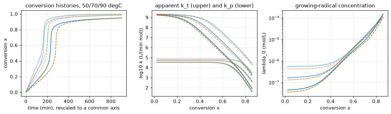
# ---- the onset construction, ROOT-FOUND and not sampled ---------------------
# Book p. 354: "The 'bend' of the log k_t curve determined by extrapolating the
# sloped region to intersect with the initial value gives a qualitative
# impression of the 'onset' of gel effect."  The paper prints no rule for which
# straight line.  RECONSTRUCTION, stated: the sloped region is represented by
# its LEAST-CURVED point - the local maximum of the second derivative of L past
# the bend, found as a root of the THIRD derivative - and the tangent there is
# extrapolated back to the
# x -> 0 value of log10 k_t, which is log10 k_t0 exactly because lambda_0(0) = 0.
def onset_from(x, L, L0, mode="flattest"):
    """The paper's graphical construction, reconstructed and root-found.

    BOTH FEATURES ARE THE **FIRST** OF THEIR KIND, NOT THE LARGEST, and that
    matters: log10 k_t has a second region of strong downward curvature at high
    conversion where the GLASS effect takes over, and for a large enough theta_t
    that second feature is the deeper one.  Taking the global minimum of the
    second derivative therefore jumps to the glass region and makes the onset
    NON-MONOTONE in theta_t.  Reading the FIRST local minimum of the second
    derivative (bend) and then the FIRST local maximum after it (the
    least-curved point of the sloped branch) picks the gel-effect feature at
    every parameter set tried.
    THE GUARD IS ON THIS FUNCTION.  `onset_window`, the derivative-free
    least-squares fit, has no curvature-feature selection and so cannot show
    this defect; and at the tabulated theta_t the two feature selections agree
    exactly.  Both constructions are asserted monotone in theta_t, in the
    leverage cell below.
    """
    cs = CubicSpline(x, L)
    d1, d2, d3 = cs.derivative(1), cs.derivative(2), cs.derivative(3)
    g = np.linspace(x[0], x[-1], 20000)
    v3 = d3(g)
    down = np.where((v3[:-1] < 0) & (v3[1:] >= 0))[0]     # first local MIN of L''
    if len(down):
        x_bend = brentq(d3, g[down[0]], g[down[0] + 1], xtol=1e-14)
    else:
        x_bend = float(g[np.argmin(d2(g))])
    gg = g[g > x_bend]
    if mode == "flattest":
        vv = d3(gg)
        up = np.where((vv[:-1] > 0) & (vv[1:] <= 0))[0]   # first local MAX of L''
        if len(up):
            xs, refined = brentq(d3, gg[up[0]], gg[up[0] + 1], xtol=1e-14), "root"
        else:
            from scipy.optimize import minimize_scalar
            rr = minimize_scalar(lambda v: -float(d2(v)),
                                 bounds=(gg[0], gg[-1]), method="bounded",
                                 options={"xatol": 1e-12})
            xs, refined = float(rr.x), "bounded"
    elif mode == "decade3":
        # ALTERNATIVE READING: the tangent taken three decades below the
        # plateau, wherever that falls.  Always exists, always root-found.
        xs = brentq(lambda v: cs(v) - (L0 - 3.0), x_bend, gg[-1], xtol=1e-14)
        refined = "root"
    elif mode == "steepest":
        # THE MOST LITERAL READING OF "the sloped region" - the tangent at the
        # steepest point of the descent - AND THE ONE READING THIS PAGE KEEPS
        # OUT OF THE DEFINITIONAL BAND, for a reason it measures rather than
        # asserts: at every one of the six conditions the steepest point sits AT
        # x = X_HI, the right edge of the window this page chose, so the reading
        # is set by where the curve is truncated and not by the curve.  The
        # interior stationary points of L' are root-found on L'' and the edge
        # competes against them explicitly, so the winner is the global steepest
        # point of the window and never a sampled one.
        v2 = d2(gg)
        cross = np.where((v2[:-1] < 0) & (v2[1:] >= 0))[0]
        cand = [brentq(d2, gg[k], gg[k + 1], xtol=1e-14) for k in cross]
        cand.append(float(gg[-1]))
        xs = min(cand, key=lambda v: float(d1(v)))
        refined = "edge" if xs == gg[-1] else "root"
    else:
        raise ValueError(mode)
    return dict(x_onset=float(xs + (L0 - cs(xs))/d1(xs)), x_tangent=float(xs),
                slope=float(d1(xs)), x_bend=float(x_bend), L_tangent=float(cs(xs)),
                refined=refined)


def onset_window(x, L, L0, lo=2.0, hi=4.0):
    """THE PRIMARY READING: the straight line least-squares-fitted to log10 k_t
    over the stated decade window L0-lo .. L0-hi, extrapolated to L0.

    It is derivative-free, so it does not have to decide which curvature
    feature is "the bend", and the intersection is exact algebra rather than a
    swept crossing.  The tangent constructions below are kept as ALTERNATIVE
    readings and their spread is reported as the definitional band.
    """
    m = (L <= L0 - lo) & (L >= L0 - hi)
    assert m.sum() >= 10, "the decade window holds too few points"
    p = np.polyfit(x[m], L[m], 1)
    return float((L0 - p[1])/p[0]), int(m.sum()), float(p[0])


def onset_x(x, L, L0, mode="window24"):
    """Dispatcher: one name for every reading of 'extrapolating the sloped region'."""
    if mode == "window24":
        return onset_window(x, L, L0, 2.0, 4.0)[0]
    if mode == "window13":
        return onset_window(x, L, L0, 1.0, 3.0)[0]
    if mode == "window35":
        return onset_window(x, L, L0, 3.0, 5.0)[0]
    if mode == "window46":
        return onset_window(x, L, L0, 4.0, 6.0)[0]
    return onset_from(x, L, L0, mode)["x_onset"]


# THE HEADLINE LOADING IS I_0 = 0.0258 mol/L AND THE CHOICE IS STATED, NOT
# IMPLIED.  The paper quotes ONE onset per temperature, but Figures 10-12 plot
# BOTH loadings and the sentence names neither; 0.0258 is the loading listed
# first in all three legends and the one Figures 16-18 plot, and that is the
# whole basis for the choice - the paper gives no other.  What the choice costs
# is measured below and printed beside the headline rather than left in the
# table: the SAME construction on the 0.01548 curve of the SAME figures misses
# the printed onsets by up to ONSET_DEV_OTHER_MAX.
I0_HEADLINE, I0_OTHER = 0.0258, 0.01548

# THE SEVEN READINGS.  Six are readings of "the sloped region" - four decade
# windows and two tangents - and the seventh reads "the initial value" the other
# way, off the post-transient plateau instead of log10 k_t^0.  An eighth,
# `steepest`, is computed and reported but deliberately NOT in the band; the
# reason is measured in the printout below.
# THE 4-6-DECADE WINDOW IS IN THE BAND BECAUSE THE PAGE'S OWN EXCLUSION TEST
# ACQUITS IT.  It is the widest-swinging reading, so leaving it out would
# flatter the band; the only ground on
# which this page excludes anything is that the reading is set by X_HI rather
# than by the curve, and that test is MEASURED below - the 4-6 window's fit mask
# ends well inside X_HI at four of the six conditions, and the band's reported
# maximum is attained at one of those four.
ONSET_READINGS = ("window24", "window13", "window35", "window46", "flattest",
                  "decade3", "plateau_L0")
ONSET = {}
for c, cv in CURVES.items():
    L0 = float(np.log10(MODELS[c].kt0))
    xo, npts, slope = onset_window(cv["x"], cv["Lt"], L0)
    o = dict(x_onset=xo, n_window=npts, slope=slope, L0=L0)
    o["alt_flattest"] = onset_from(cv["x"], cv["Lt"], L0)["x_onset"]
    o["alt_decade3"] = onset_from(cv["x"], cv["Lt"], L0, "decade3")["x_onset"]
    o["alt_window_1_3"] = onset_window(cv["x"], cv["Lt"], L0, 1.0, 3.0)[0]
    o["alt_window_3_5"] = onset_window(cv["x"], cv["Lt"], L0, 3.0, 5.0)[0]
    o["alt_window_4_6"] = onset_window(cv["x"], cv["Lt"], L0, 4.0, 6.0)[0]
    # WHERE THE 4-6-DECADE WINDOW'S FIT MASK ENDS.  Measured, because "the
    # reading is set by X_HI and not by the curve" is the only ground on which
    # this page keeps any reading out of the band, and it has to be applied to
    # this window as well as to the steepest tangent.
    _m46 = (cv["Lt"] <= L0 - 4.0) & (cv["Lt"] >= L0 - 6.0)
    o["x_window_4_6_hi"] = float(cv["x"][_m46].max())
    o["window_4_6_interior"] = bool(o["x_window_4_6_hi"] < X_HI - 1e-9)
    # the seventh reading: the "initial value" taken as the post-transient plateau
    o["alt_plateau_L0"] = onset_window(cv["x"], cv["Lt"], float(cv["Lt"][0]))[0]
    _st_ = onset_from(cv["x"], cv["Lt"], L0, "steepest")
    o["alt_steepest"] = _st_["x_onset"]
    o["steepest_x_tangent"] = _st_["x_tangent"]
    o["steepest_at_edge"] = bool(_st_["refined"] == "edge")
    _alts = [o["x_onset"], o["alt_window_1_3"], o["alt_window_3_5"],
             o["alt_window_4_6"], o["alt_flattest"], o["alt_decade3"],
             o["alt_plateau_L0"]]
    o["band"] = float(max(_alts) - min(_alts))
    # the band without the 4-6-decade window, for the break table
    _six = [o["x_onset"], o["alt_window_1_3"], o["alt_flattest"],
            o["alt_decade3"], o["alt_plateau_L0"], o["alt_window_3_5"]]
    o["band_six_readings"] = float(max(_six) - min(_six))
    ONSET[c] = o

_st = TS.set_index("key")
ONSET_PRINTED = {TC: float(_st.loc[f"onset_conversion_{TC}C", "value"])
                 for TC in (50, 70, 90)}
print("gel-effect onset conversion - the paper's graphical construction,"
      " reconstructed and root-found\n")
print(f"{'T':>4} {'I0':>9} {'x_onset':>9} {'printed':>8} {'dev':>9}"
      f" {'n pts':>7} {'slope':>8} {'defn band':>10}")
for c in CONDITIONS:
    o, pr = ONSET[c], ONSET_PRINTED[c[0]]
    print(f"{c[0]:4d} {c[1]:9g} {o['x_onset']:9.5f} {pr:8.2f}"
          f" {o['x_onset'] - pr:+9.5f} {o['n_window']:7d}"
          f" {o['slope']:8.3f} {o['band']:10.5f}")
ONSET_DEV = {TC: ONSET[(TC, I0_HEADLINE)]["x_onset"] - ONSET_PRINTED[TC]
             for TC in (50, 70, 90)}
ONSET_DEV_OTHER = {TC: ONSET[(TC, I0_OTHER)]["x_onset"] - ONSET_PRINTED[TC]
                   for TC in (50, 70, 90)}
ONSET_MAX_ABS_DEV = float(max(abs(v) for v in ONSET_DEV.values()))
ONSET_DEV_OTHER_MAX = float(max(abs(v) for v in ONSET_DEV_OTHER.values()))
ONSET_MAX_BAND = float(max(ONSET[c]["band"] for c in CONDITIONS))
ONSET_BAND_SIX = float(max(ONSET[c]["band_six_readings"] for c in CONDITIONS))
ONSET_I0_SHIFT = {TC: abs(ONSET[(TC, I0_HEADLINE)]["x_onset"]
                          - ONSET[(TC, I0_OTHER)]["x_onset"])
                  for TC in (50, 70, 90)}
ONSET_I0_MAX = float(max(ONSET_I0_SHIFT.values()))
print(f"\nthe {len(ONSET_READINGS)} readings, at each condition:\n")
print(f"{'T':>4} {'I0':>9} {'win 2-4':>9} {'win 1-3':>9} {'win 3-5':>9}"
      f" {'win 4-6':>9} {'flattest':>9} {'3-decade':>9} {'plateau':>9}"
      f" {'band':>9}")
for c in CONDITIONS:
    o = ONSET[c]
    print(f"{c[0]:4d} {c[1]:9g} {o['x_onset']:9.5f} {o['alt_window_1_3']:9.5f}"
          f" {o['alt_window_3_5']:9.5f} {o['alt_window_4_6']:9.5f}"
          f" {o['alt_flattest']:9.5f}"
          f" {o['alt_decade3']:9.5f} {o['alt_plateau_L0']:9.5f}"
          f" {o['band']:9.5f}")
print(f"\nmax |model - printed| at I_0 = {I0_HEADLINE:g} mol/L (the headline"
      f" loading) = {ONSET_MAX_ABS_DEV:.5f} in conversion")
print(f"THE SAME CONSTRUCTION ON THE OTHER LOADING OF THE SAME FIGURES misses"
      f" by up to {ONSET_DEV_OTHER_MAX:.5f}")
print(f"  ({', '.join(f'{TC} degC {ONSET_DEV_OTHER[TC]:+.5f}' for TC in (50, 70, 90))})"
      f" - {ONSET_DEV_OTHER_MAX/ONSET_MAX_ABS_DEV:.2f}x the headline miss.  The"
      f" paper quotes one onset per\n  temperature and gives no basis for"
      f" preferring either curve, so BOTH are printed and the\n  headline says"
      f" which it uses.")
print(f"\nwidest spread over the {len(ONSET_READINGS)} readings ="
      f" {ONSET_MAX_BAND:.5f}"
      f"  ({ONSET_MAX_BAND/ONSET_MAX_ABS_DEV:.2f}x the largest miss)")
print(f"  THE BAND IS NOT CHOSEN TO FLATTER: nothing is kept out of it that this"
      f" page cannot exclude on\n  a measurement.")
print(f"largest shift between the two initiator loadings ="
      f" {ONSET_I0_MAX:.5f}   <- the paper: 'initiator loading has very little"
      f" effect on both curves'")
# THE READING THE BAND DOES NOT COVER, NAMED AND PRICED RATHER THAN OMITTED.
ONSET_STEEPEST_MAX = float(max(ONSET[c]["alt_steepest"] for c in CONDITIONS))
N_STEEPEST_AT_EDGE = int(sum(ONSET[c]["steepest_at_edge"] for c in CONDITIONS))
N_W46_INTERIOR = int(sum(ONSET[c]["window_4_6_interior"] for c in CONDITIONS))
print(f"\nTHE SAME TEST, APPLIED TO THE READING THAT WAS ADMITTED RATHER THAN"
      f" EXCLUDED.  The 4-6-decade\nwindow gives"
      f" {', '.join(f'{ONSET[(TC, I0_HEADLINE)]['alt_window_4_6']:.5f}' for TC in (50, 70, 90))}"
      f" at 50/70/90 degC and is the widest-swinging reading in the\nband, so"
      f" leaving it out would be the flattering choice - and the exclusion test"
      f" ACQUITS it: its fit\nmask ends at"
      f" {', '.join(f'{ONSET[c]['x_window_4_6_hi']:.4f}' for c in CONDITIONS)},"
      f" i.e. INSIDE x = {X_HI:g} at {N_W46_INTERIOR} of the"
      f" {len(CONDITIONS)} conditions,\nand the band's reported maximum"
      f" {ONSET_MAX_BAND:.5f} is attained at one of those"
      f" {N_W46_INTERIOR} - so the number\nabove is not set by the truncation"
      f" either.  It touches the edge only at 90 degC, where the\npaper's own"
      f" Figure 12 runs to about 0.96 and would not truncate it at all.")
assert N_W46_INTERIOR >= 4 and ONSET[max(
    CONDITIONS, key=lambda c: ONSET[c]["band"])]["window_4_6_interior"], (
    "the 4-6-decade window's fit mask now reaches the window edge where the band"
    " is widest, so the reason for admitting it rather than excluding it - the"
    " same truncation test the steepest-slope tangent fails - no longer holds")
print(f"\nAND THE BAND IS A SPREAD OVER {len(ONSET_READINGS)} READINGS, NOT A"
      f" BOUND OVER EVERY"
      f" READING OF THE SENTENCE.\nThe most literal reading - the tangent at the"
      f" STEEPEST point of the descent - gives"
      f"\n  {', '.join(f'{ONSET[(TC, I0_HEADLINE)]['alt_steepest']:.5f}' for TC in (50, 70, 90))}"
      f" at 50/70/90 degC, outside the band at every condition.  IT IS EXCLUDED"
      f"\n  FOR A MEASURED REASON: its tangent point sits at x = {X_HI:g}, the"
      f" right edge of this page's\n  own window, at {N_STEEPEST_AT_EDGE} of the"
      f" {len(CONDITIONS)} conditions - so that reading is set by where the"
      f" curve is\n  TRUNCATED and not by the curve.  Figures 11 and 12 run"
      f" further right than Figure 10 does,\n  so the paper's own plots would"
      f" not place it there.")
assert all(ONSET[c]["steepest_at_edge"] for c in CONDITIONS), (
    "the steepest-slope tangent no longer sits at the window edge, so the stated"
    " reason for keeping it out of the definitional band no longer holds")
assert (ONSET[(50, I0_HEADLINE)]["x_onset"] < ONSET[(70, I0_HEADLINE)]["x_onset"]
        < ONSET[(90, I0_HEADLINE)]["x_onset"]), "the printed trend with T is not reproduced"
gel-effect onset conversion - the paper's graphical construction, reconstructed and root-found
T I0 x_onset printed dev n pts slope defn band
50 0.0258 0.25516 0.26 -0.00484 866 -11.052 0.05848
50 0.01548 0.23760 0.26 -0.02240 881 -10.877 0.04665
70 0.0258 0.34838 0.35 -0.00162 865 -11.022 0.09009
70 0.01548 0.32167 0.35 -0.02833 890 -10.719 0.08444
90 0.0258 0.44034 0.45 -0.00966 829 -11.448 0.07740
90 0.01548 0.41874 0.45 -0.03126 854 -11.139 0.07782
the 7 readings, at each condition:
T I0 win 2-4 win 1-3 win 3-5 win 4-6 flattest 3-decade plateau band
50 0.0258 0.25516 0.24109 0.25761 0.29957 0.25453 0.25718 0.25996 0.05848
50 0.01548 0.23760 0.22396 0.23478 0.27061 0.23507 0.23995 0.24332 0.04665
70 0.0258 0.34838 0.32990 0.36832 0.41999 0.34976 0.34932 0.35121 0.09009
70 0.01548 0.32167 0.30435 0.33514 0.38878 0.32318 0.32317 0.32533 0.08444
90 0.0258 0.44034 0.41775 0.46901 0.49516 0.43888 0.44079 0.44199 0.07740
90 0.01548 0.41874 0.39733 0.44404 0.47515 0.41948 0.41949 0.42083 0.07782
max |model - printed| at I_0 = 0.0258 mol/L (the headline loading) = 0.00966 in conversion
THE SAME CONSTRUCTION ON THE OTHER LOADING OF THE SAME FIGURES misses by up to 0.03126
(50 degC -0.02240, 70 degC -0.02833, 90 degC -0.03126) - 3.24x the headline miss. The paper quotes one onset per
temperature and gives no basis for preferring either curve, so BOTH are printed and the
headline says which it uses.
widest spread over the 7 readings = 0.09009 (9.33x the largest miss)
THE BAND IS NOT CHOSEN TO FLATTER: nothing is kept out of it that this page cannot exclude on
a measurement.
largest shift between the two initiator loadings = 0.02671 <- the paper: 'initiator loading has very little effect on both curves'
THE SAME TEST, APPLIED TO THE READING THAT WAS ADMITTED RATHER THAN EXCLUDED. The 4-6-decade
window gives 0.29957, 0.41999, 0.49516 at 50/70/90 degC and is the widest-swinging reading in the
band, so leaving it out would be the flattering choice - and the exclusion test ACQUITS it: its fit
mask ends at 0.7766, 0.7733, 0.8568, 0.8484, 0.8600, 0.8600, i.e. INSIDE x = 0.86 at 4 of the 6 conditions,
and the band's reported maximum 0.09009 is attained at one of those 4 - so the number
above is not set by the truncation either. It touches the edge only at 90 degC, where the
paper's own Figure 12 runs to about 0.96 and would not truncate it at all.
AND THE BAND IS A SPREAD OVER 7 READINGS, NOT A BOUND OVER EVERY READING OF THE SENTENCE.
The most literal reading - the tangent at the STEEPEST point of the descent - gives
0.44783, 0.47680, 0.51866 at 50/70/90 degC, outside the band at every condition. IT IS EXCLUDED
FOR A MEASURED REASON: its tangent point sits at x = 0.86, the right edge of this page's
own window, at 6 of the 6 conditions - so that reading is set by where the curve is
TRUNCATED and not by the curve. Figures 11 and 12 run further right than Figure 10 does,
so the paper's own plots would not place it there.# ---- SECOND, INDEPENDENT ROUTE to the same curve: integrate in x -------------
# The same six ODEs re-parametrised by conversion - divide eq. 10 and 12 by
# eq. 11 - so the independent variable, the step sequence and the error control
# are all different. It shares the state at x = X_LO_FIT with the t-route and
# therefore tests the integration over the sloped branch, NOT the start-up.
def curve_x(model, nx=4001, x_lo=X_LO_FIT, x_hi=X_HI, rtol=1e-10, y_start=None):
if y_start is None:
cv = CURVES[(int(model.T_C), model.I0)]
y_start = (float(cv["sol"].sol(cv["t"][0])[0]), float(cv["lam0"][0]))
def rhs_x(x, y):
I, l0 = y
kt, kp = model.kt_kp(x, l0)
dxdt = kp*(1.0 - x)*l0
dil = model.eps*(1.0 - x)*kp*l0/(1.0 + model.eps*x)
return [(-model.kd*I - dil*I)/dxdt,
(-dil*l0 + 2.0*F_EFF*model.kd*I - kt*l0*l0)/dxdt]
xs = np.linspace(x_lo, x_hi, nx)
s = solve_ivp(rhs_x, (x_lo, x_hi), list(y_start), method="Radau",
rtol=rtol, atol=1e-18, t_eval=xs)
assert s.success, "x-parametrised solve failed"
kt = np.array([model.kt_kp(xi, pi)[0] for xi, pi in zip(xs, s.y[1])])
return xs, np.log10(kt), s.y[1]
ONSET_X_ROUTE, ONSET_TWO_ROUTE = {}, {}
for c in CONDITIONS:
xs, Lt, l0 = curve_x(MODELS[c])
ONSET_X_ROUTE[c] = onset_x(xs, Lt, ONSET[c]["L0"])
ONSET_TWO_ROUTE[c] = abs(ONSET_X_ROUTE[c]/ONSET[c]["x_onset"] - 1.0)
ONSET_TWO_ROUTE_MAX = float(max(ONSET_TWO_ROUTE.values()))
print("t-parametrised vs x-parametrised integration, same onset construction:")
for c in CONDITIONS:
print(f" {c[0]:2d} degC, I0 = {c[1]:<8g} t-route {ONSET[c]['x_onset']:.6f}"
f" x-route {ONSET_X_ROUTE[c]:.6f} rel {ONSET_TWO_ROUTE[c]:.3e}")
# WHAT THAT RESIDUAL MEASURES, AND WHAT IT DOES NOT. It is NOT the arithmetic
# floor of the onset. lambda_0(x) sits on a strongly attracting manifold, so
# two integrations of the same equations converge onto the same log k_t(x)
# whatever path they took to get there; the residual therefore prices the
# ATTRACTOR - that both parametrisations land on the same constitutive curve -
# and not the accuracy of either integration. The floor that does limit the
# printed digits is the RESAMPLING of that curve onto a uniform grid in x, and
# it is measured here instead of assumed.
ONSET_NX = [2001, 4001, 8001, 16001]
ONSET_NX_VALS = {}
for TC in (50, 70, 90):
vals = []
for nx in ONSET_NX:
cv = (CURVES[(TC, I0_HEADLINE)] if nx == 4001
else curve(MODELS[(TC, I0_HEADLINE)], nx=nx))
vals.append(onset_x(cv["x"], cv["Lt"], ONSET[(TC, I0_HEADLINE)]["L0"]))
ONSET_NX_VALS[TC] = vals
def _resample_floor(vals_by_TC, ks):
return float(max((max(v[k] for k in ks) - min(v[k] for k in ks))
/ abs(v[ks[0]]) for v in vals_by_TC.values()))
ONSET_RESAMPLE_FLOOR = _resample_floor(ONSET_NX_VALS, list(range(len(ONSET_NX))))
print(f"\nthe onset against the RESAMPLING grid (nx points uniform in x over"
f" [{X_LO_FIT:g}, {X_HI:g}]):\n")
print(f"{'T':>4} " + " ".join(f"{'nx=' + str(n):>13}" for n in ONSET_NX)
+ f" {'spread':>10}")
for TC in (50, 70, 90):
v = ONSET_NX_VALS[TC]
print(f"{TC:4d} " + " ".join(f"{x:13.9f}" for x in v)
+ f" {max(v) - min(v):10.2e}")
print(f"\n RELATIVE SPREAD OVER THE FOUR GRIDS: {ONSET_RESAMPLE_FLOOR:.3e} - at"
f" least five orders of magnitude larger than\n the gap between the two"
f" integration routes, below 1e-10 (here {ONSET_TWO_ROUTE_MAX:.1e}). So the"
f" arithmetic floor on the onset\n is the resampling, the sixth decimal"
f" of every onset printed on this page is grid noise,\n and the page"
f" quotes five. Both floors are far inside the"
f" {ONSET_MAX_BAND:.5f} definitional band,\n which is what actually"
f" limits the number.")
# and the start-up itself, pinned against the algebraic quasi-steady value
QSS_START_REL = {}
for c in CONDITIONS:
cv, m = CURVES[c], MODELS[c]
I_at = float(cv["sol"].sol(cv["t"][0])[0])
QSS_START_REL[c] = abs(m.lam0_qssa(X_LO_FIT, I_at)/cv["lam0"][0] - 1.0)
QSS_START_MAX = float(max(QSS_START_REL.values()))
print(f"\nthe shared start state is pinned separately: at x = {X_LO_FIT}, the"
f" marched lambda_0 is\nwithin {QSS_START_MAX:.3e} of the ALGEBRAIC"
f" quasi-steady root of eq. 12 - so the piece the two\nroutes share is"
f" itself checked against a root-find that shares no time stepping.")t-parametrised vs x-parametrised integration, same onset construction:
50 degC, I0 = 0.0258 t-route 0.255161 x-route 0.255161 rel 9.077e-12
50 degC, I0 = 0.01548 t-route 0.237599 x-route 0.237599 rel 6.691e-12
70 degC, I0 = 0.0258 t-route 0.348378 x-route 0.348378 rel 3.836e-13
70 degC, I0 = 0.01548 t-route 0.321672 x-route 0.321672 rel 5.324e-12
90 degC, I0 = 0.0258 t-route 0.440339 x-route 0.440339 rel 5.208e-13
90 degC, I0 = 0.01548 t-route 0.418739 x-route 0.418739 rel 8.207e-13
the onset against the RESAMPLING grid (nx points uniform in x over [0.02, 0.86]):
T nx=2001 nx=4001 nx=8001 nx=16001 spread
50 0.255163107 0.255161103 0.255163192 0.255163689 2.59e-06
70 0.348375921 0.348377542 0.348378352 0.348378757 2.84e-06
90 0.440338593 0.440338511 0.440338468 0.440344242 5.77e-06
RELATIVE SPREAD OVER THE FOUR GRIDS: 1.311e-05 - at least five orders of magnitude larger than
the gap between the two integration routes, below 1e-10 (here 9.1e-12). So the arithmetic floor on the onset
is the resampling, the sixth decimal of every onset printed on this page is grid noise,
and the page quotes five. Both floors are far inside the 0.09009 definitional band,
which is what actually limits the number.
the shared start state is pinned separately: at x = 0.02, the marched lambda_0 is
within 7.362e-06 of the ALGEBRAIC quasi-steady root of eq. 12 - so the piece the two
routes share is itself checked against a root-find that shares no time stepping.# ---- Figure 13's activation energies, recomputed from Table II --------------
def arrhenius(theta, T_K):
"""least squares of ln(1/theta) on 1/T; returns E in kcal/mol."""
y = np.log(1.0/np.asarray(theta, float))
X = np.vstack([np.ones_like(T_K), 1.0/T_K]).T
c, *_ = np.linalg.lstsq(X, y, rcond=None)
res = y - X @ c
return (-c[1]*R_CAL/1000.0, float(np.sqrt((res**2).mean())),
float(np.max(np.abs(res))))
TK3 = np.array([50.0, 70.0, 90.0]) + 273.15
TH_T = {I0: np.array([float(T2[(T2.polym_temp_C == TC)
& np.isclose(T2.initiator_loading_mol_per_L, I0)]
.theta_t_min.iloc[0]) for TC in (50, 70, 90)])
for I0 in (0.0258, 0.01548)}
TH_P = np.array([float(T2[T2.polym_temp_C == TC].theta_p_min.iloc[0])
for TC in (50, 70, 90)])
E_T = {I0: arrhenius(v, TK3) for I0, v in TH_T.items()}
E_P = arrhenius(TH_P, TK3)
E_T_PRINTED = float(_st.loc["activation_energy_theta_t", "value"])
E_P_PRINTED = float(_st.loc["activation_energy_theta_p", "value"])
E_T_MEAN = float(np.mean([E_T[i][0] for i in TH_T]))
print("Arrhenius fits to Table II's own theta values (Figure 13):")
for I0 in (0.0258, 0.01548):
E, rms, mx = E_T[I0]
print(f" theta_t, I0 = {I0:<8g} dE = {E:7.4f} kcal/mol ln-residual"
f" rms {rms:.5f} max {mx:.5f} vs printed {E_T_PRINTED:g}"
f" ({E/E_T_PRINTED - 1:+.2%})")
print(f" theta_p dE = {E_P[0]:7.4f} kcal/mol ln-residual"
f" rms {E_P[1]:.5f} max {E_P[2]:.5f} vs printed {E_P_PRINTED:g}"
f" ({E_P[0]/E_P_PRINTED - 1:+.2%})")
E_T_REL = {I0: abs(E_T[I0][0]/E_T_PRINTED - 1.0) for I0 in TH_T}
E_P_REL = abs(E_P[0]/E_P_PRINTED - 1.0)
print(f"\nboth loadings' theta_t lines average {E_T_MEAN:.4f} kcal/mol"
f" ({E_T_MEAN/E_T_PRINTED - 1:+.2%} on the printed {E_T_PRINTED:g}).")Arrhenius fits to Table II's own theta values (Figure 13):
theta_t, I0 = 0.0258 dE = 34.9082 kcal/mol ln-residual rms 0.12159 max 0.17186 vs printed 34 (+2.67%)
theta_t, I0 = 0.01548 dE = 34.5166 kcal/mol ln-residual rms 0.09702 max 0.13713 vs printed 34 (+1.52%)
theta_p dE = 27.7716 kcal/mol ln-residual rms 0.05687 max 0.08038 vs printed 28 (-0.82%)
both loadings' theta_t lines average 34.7124 kcal/mol (+2.10% on the printed 34).# ---- Figure 15's claim, tested on Table I's T_gp and Table II's A -----------
# Figure 15 caption: "All three points fall on the same straight line".
A3 = np.array([float(T2[T2.polym_temp_C == TC].A.iloc[0]) for TC in (50, 70, 90)])
TC3 = np.array([50.0, 70.0, 90.0])
U = (TC3 - T_GP)**2
_X = np.vstack([np.ones_like(U), U]).T
_c, *_ = np.linalg.lstsq(_X, A3, rcond=None)
A_RESID = A3 - _X @ _c
A_LIN_MAXREL = float(np.max(np.abs(A_RESID/A3)))
# NULL BASELINE: the same three points, two parameters, a different regressor
_X1 = np.vstack([np.ones_like(TC3), TC3]).T
_c1, *_ = np.linalg.lstsq(_X1, A3, rcond=None)
A_NULL_T_MAXREL = float(np.max(np.abs((A3 - _X1 @ _c1)/A3)))
A_NULL_GAIN = A_NULL_T_MAXREL/A_LIN_MAXREL
# what T_gp would make the three points EXACTLY collinear
def _collinear(Tg):
u = (TC3 - Tg)**2
return (A3[1] - A3[0])*(u[2] - u[1]) - (A3[2] - A3[1])*(u[1] - u[0])
T_GP_IMPLIED = float(brentq(_collinear, 50.0, 200.0, xtol=1e-12))
# ... and what the printed rounding of A alone allows
_lo, _hi = np.inf, -np.inf
for d0 in (-5e-4, 0.0, 5e-4):
for d1 in (-5e-4, 0.0, 5e-4):
for d2 in (-5e-4, 0.0, 5e-4):
Ap = A3 + np.array([d0, d1, d2])
def _g(Tg, Ap=Ap):
u = (TC3 - Tg)**2
return (Ap[1] - Ap[0])*(u[2] - u[1]) - (Ap[2] - Ap[1])*(u[1] - u[0])
try:
v = brentq(_g, -1e3, 1e3, xtol=1e-10)
_lo, _hi = min(_lo, v), max(_hi, v)
except ValueError:
pass
T_GP_BAND_LO, T_GP_BAND_HI = float(_lo), float(_hi)
# and which EXPONENT the three points actually pick out, at the printed T_gp
def _expo(q):
u = (T_GP - TC3)**q
return (A3[1] - A3[0])*(u[2] - u[1]) - (A3[2] - A3[1])*(u[1] - u[0])
Q_IMPLIED = float(brentq(_expo, 0.3, 6.0, xtol=1e-12))
# WHAT THE 17.4x IS A FUNCTION OF, AND WHAT SURVIVES ITS BEING ONE. The gain is
# a strong function of T_gp, and this page has already shown that the three
# printed A values cannot determine T_gp. So the gain is evaluated at the two
# ENDS of the admissible interval as well as at the printed 114 - four exact
# evaluations, no extremum claimed - and beside two OTHER two-parameter,
# non-nested regressors on the same three points.
def _gain_at(Tg):
u = (TC3 - Tg)**2
Xg = np.vstack([np.ones_like(u), u]).T
cg, *_ = np.linalg.lstsq(Xg, A3, rcond=None)
lin = float(np.max(np.abs((A3 - Xg @ cg)/A3)))
return A_NULL_T_MAXREL/lin if lin else np.inf
def _maxrel_on(X):
cc, *_ = np.linalg.lstsq(X, A3, rcond=None)
return float(np.max(np.abs((A3 - X @ cc)/A3)))
A_GAIN_BAND_LO = _gain_at(T_GP_BAND_LO)
A_GAIN_BAND_HI = _gain_at(T_GP_BAND_HI)
A_GAIN_BAND_ENDS_MIN = float(min(A_GAIN_BAND_LO, A_GAIN_BAND_HI))
A_ALT_CENTRE = 130.0 # an arbitrary alternative centre, stated as one
A_ALT_REGRESSORS = {
"A against 1/T (degC)": np.vstack([np.ones_like(TC3), 1.0/TC3]).T,
f"A against (T - {A_ALT_CENTRE:g})^2":
np.vstack([np.ones_like(TC3), (TC3 - A_ALT_CENTRE)**2]).T,
}
A_ALT_GAIN = {k: A_NULL_T_MAXREL/_maxrel_on(X) for k, X in A_ALT_REGRESSORS.items()}
A_ALT_GAIN_MAX = float(max(A_ALT_GAIN.values()))
# the three A values are equally spaced in T, so their second difference IS the
# discrete curvature, and it is what any of these regressors is picking up.
A_SECOND_DIFF = float(A3[0] - 2.0*A3[1] + A3[2])
print(f"A against (T - T_gp)^2 with T_gp = {T_GP:g} degC as Table I prints it:")
print(f" least-squares line A = {_c[0]:.6f} {_c[1]:+.6e} (T-T_gp)^2")
print(f" residuals {np.array2string(A_RESID, precision=8)}")
print(f" max relative residual {A_LIN_MAXREL:.3e} <- 'all three points fall on"
f" the same straight line'")
print(f" NULL, A linear in T {A_NULL_T_MAXREL:.3e} ({A_NULL_GAIN:.4f}x worse;"
f" not a nested submodel, so the direction is evidence)")
print(f"\n T_gp making the three A values EXACTLY collinear:"
f" {T_GP_IMPLIED:.5f} degC")
print(f" T_gp still admissible if each printed A is +-0.0005:"
f" [{T_GP_BAND_LO:.4f}, {T_GP_BAND_HI:.4f}] degC")
print(f" -> the printed {T_GP:g} degC sits inside that interval, so the three"
f" rounded A values\n CANNOT distinguish it from {T_GP_IMPLIED:.2f};"
f" the page reports the interval, not the point.")
print(f" exponent q making A exactly linear in (T_gp - T)^q at the printed"
f" T_gp: {Q_IMPLIED:.5f}")
print(f"\n AND THE GAIN IS A FUNCTION OF T_gp, WHICH THESE THREE CELLS CANNOT"
f" DETERMINE. Evaluated at\n the two ends of the interval they DO admit:"
f" {A_GAIN_BAND_LO:.4f}x at {T_GP_BAND_LO:.4f} degC and"
f" {A_GAIN_BAND_HI:.4f}x at\n {T_GP_BAND_HI:.4f} degC, against"
f" {A_NULL_GAIN:.4f}x at the printed {T_GP:g}; and it DIVERGES at"
f" {T_GP_IMPLIED:.5f} degC,\n where the residual is exactly zero by"
f" construction. So {A_NULL_GAIN:.4f}x is the gain at ONE admissible"
f"\n T_gp and not a property of the data.")
for k_, v_ in A_ALT_GAIN.items():
print(f" {k_:24s} max rel residual {_maxrel_on(A_ALT_REGRESSORS[k_]):.3e}"
f" gain vs linear-in-T {v_:.4f}x")
print(f"\n BOTH OF THOSE ARE TWO-PARAMETER AND NEITHER NESTS IN linear-in-T"
f" EITHER, so the comparison\n does NOT single out the"
f" Fujita/glass-transition form. What it establishes is that A is"
f"\n CONCAVE in T - the three values are equally spaced in T and their"
f" second difference is\n {A_SECOND_DIFF:+.6f} - which linear-in-T cannot"
f" represent and any sufficiently curved\n two-parameter regressor can."
f" The page claims the concavity, not the quadratic.")
assert T_GP_BAND_LO < T_GP < T_GP_BAND_HI
assert A_SECOND_DIFF < 0 and A_GAIN_BAND_ENDS_MIN > 1.0A against (T - T_gp)^2 with T_gp = 114 degC as Table I prints it:
least-squares line A = 0.167833 -8.247292e-06 (T-T_gp)^2
residuals [-5.17941774e-05 1.34055518e-04 -8.22613406e-05]
max relative residual 8.819e-04 <- 'all three points fall on the same straight line'
NULL, A linear in T 1.535e-02 (17.4057x worse; not a nested submodel, so the direction is evidence)
T_gp making the three A values EXACTLY collinear: 111.42857 degC
T_gp still admissible if each printed A is +-0.0005: [102.2222, 128.0000] degC
-> the printed 114 degC sits inside that interval, so the three rounded A values
CANNOT distinguish it from 111.43; the page reports the interval, not the point.
exponent q making A exactly linear in (T_gp - T)^q at the printed T_gp: 2.06586
AND THE GAIN IS A FUNCTION OF T_gp, WHICH THESE THREE CELLS CANNOT DETERMINE. Evaluated at
the two ends of the interval they DO admit: 3.6124x at 102.2222 degC and 3.5347x at
128.0000 degC, against 17.4057x at the printed 114; and it DIVERGES at 111.42857 degC,
where the residual is exactly zero by construction. So 17.4057x is the gain at ONE admissible
T_gp and not a property of the data.
A against 1/T (degC) max rel residual 2.745e-03 gain vs linear-in-T 5.5926x
A against (T - 130)^2 max rel residual 4.708e-03 gain vs linear-in-T 3.2607x
BOTH OF THOSE ARE TWO-PARAMETER AND NEITHER NESTS IN linear-in-T EITHER, so the comparison
does NOT single out the Fujita/glass-transition form. What it establishes is that A is
CONCAVE in T - the three values are equally spaced in T and their second difference is
-0.007000 - which linear-in-T cannot represent and any sufficiently curved
two-parameter regressor can. The page claims the concavity, not the quadratic.# ---- the quasi-steady-state assumption, book p. 356 -------------------------
QSSA = {}
for c in CONDITIONS:
m = MODELS[c]
te = T_END[c[0]]
se, sq = m.solve(te), m.solve_qssa(te)
tg = np.linspace(1.0, te, 20001) # t >= 1 min: past the radical build-up
Ye, Yq = se.sol(tg), sq.sol(tg)
l0q = np.array([m.lam0_qssa(min(max(x, 0.0), 1 - 1e-12), I)
for x, I in zip(Yq[1], Yq[0])])
ratio = l0q/Ye[2]
i = int(np.argmax(ratio))
QSSA[c] = dict(max_ratio=float(ratio.max()), x_at_max=float(Ye[1][i]),
t_at_max=float(tg[i]), end_ratio=float(ratio[-1]),
max_dx=float(np.max(np.abs(Yq[1] - Ye[1]))),
x_end_exact=float(Ye[1][-1]), x_end_qssa=float(Yq[1][-1]))
QSSA_FACTOR_PRINTED = float(_st.loc["qssa_radical_overestimate_factor", "value"])
print("QSSA against the exact solution (t >= 1 min, past the radical build-up):\n")
print(f"{'T':>4} {'I0':>9} {'max lam0 QSSA/exact':>21} {'at x':>8}"
f" {'max |dx|':>10} {'x_end exact':>12} {'x_end QSSA':>11}")
for c in CONDITIONS:
q = QSSA[c]
print(f"{c[0]:4d} {c[1]:9g} {q['max_ratio']:21.4f} {q['x_at_max']:8.4f}"
f" {q['max_dx']:10.5f} {q['x_end_exact']:12.5f} {q['x_end_qssa']:11.5f}")
QSSA_REF = QSSA[(50, 0.0258)] # the condition of Figures 16-18
print(f"\nFigures 16-18 are PMMA at 50 degC, I0 = 0.0258 mol/L - this row:")
print(f" radical concentration overestimated by up to"
f" {QSSA_REF['max_ratio']:.4f}x, and the paper says 'more than a factor of"
f" {QSSA_FACTOR_PRINTED:g}'.")
print(f" conversion history differs by at most {QSSA_REF['max_dx']:.5f} in x -"
f" 'surprisingly consistent'.")
QSSA_OTHER_MAX = float(max(QSSA[c]["max_ratio"] for c in CONDITIONS
if c[0] != 50))
QSSA_N_ABOVE = int(sum(QSSA[c]["max_ratio"] > QSSA_FACTOR_PRINTED
for c in CONDITIONS))
_above = [c for c in CONDITIONS if QSSA[c]["max_ratio"] > QSSA_FACTOR_PRINTED]
_below = [c for c in CONDITIONS if QSSA[c]["max_ratio"] <= QSSA_FACTOR_PRINTED]
print(f"\n THE PAPER STATES THAT FACTOR FOR ONE CONDITION AND THIS PAGE"
f" MEASURES ALL SIX. It holds at\n {QSSA_N_ABOVE} of them"
f" - {', '.join(f'{c[0]} degC/{c[1]:g}' for c in _above)} - and FAILS at"
f" the other {len(_below)}:\n "
f"{', '.join(f'{c[0]} degC/{c[1]:g} at {QSSA[c][chr(34)+chr(34)] if False else QSSA[c]['max_ratio']:.4f}x' for c in _below)}."
f"\n The factor falls with temperature and rises as the initiator"
f" loading falls, so the\n paper's sentence is a statement about its own"
f" Figure 16 and not about the model.")
assert QSSA_REF["max_ratio"] > QSSA_FACTOR_PRINTEDQSSA against the exact solution (t >= 1 min, past the radical build-up):
T I0 max lam0 QSSA/exact at x max |dx| x_end exact x_end QSSA
50 0.0258 3.5176 0.6984 0.03861 0.94882 0.94891
50 0.01548 4.8466 0.6991 0.05143 0.94651 0.94665
70 0.0258 1.9342 0.7497 0.01896 0.98595 0.98597
70 0.01548 2.5481 0.7502 0.02850 0.98508 0.98513
90 0.0258 1.4889 0.7959 0.01099 0.99726 0.99727
90 0.01548 1.7875 0.7998 0.01662 0.99684 0.99686
Figures 16-18 are PMMA at 50 degC, I0 = 0.0258 mol/L - this row:
radical concentration overestimated by up to 3.5176x, and the paper says 'more than a factor of 2'.
conversion history differs by at most 0.03861 in x - 'surprisingly consistent'.
THE PAPER STATES THAT FACTOR FOR ONE CONDITION AND THIS PAGE MEASURES ALL SIX. It holds at
3 of them - 50 degC/0.0258, 50 degC/0.01548, 70 degC/0.01548 - and FAILS at the other 3:
70 degC/0.0258 at 1.9342x, 90 degC/0.0258 at 1.4889x, 90 degC/0.01548 at 1.7875x.
The factor falls with temperature and rises as the initiator loading falls, so the
paper's sentence is a statement about its own Figure 16 and not about the model.# ---- the paper's own argument against a switched-on gel effect ---------------
# Book p. 353: "Note that these curves are concave upward preceding the sharp
# rise. If the gel effect were suddenly switched on at a certain critical
# conversion level, the portion of the conversion curve under examination would
# be concave downward due to the gradual depletion of monomer."
def concavity(model, t_end, n=200001, t_lo=0.5):
s = model.solve(t_end)
tg = np.linspace(t_lo, t_end, n)
cs = CubicSpline(tg, s.sol(tg)[1])
d2 = cs.derivative(2)(tg)
sgn = np.where(np.diff(np.sign(d2)) != 0)[0]
return cs, tg, d2, sgn
CONCAVE = {}
for c in CONDITIONS:
cs, tg, d2, sgn = concavity(MODELS[c], T_END[c[0]])
xs = [float(cs(tg[k])) for k in sgn]
CONCAVE[c] = dict(x_sign_changes=xs[:3], x_up_from=xs[0] if xs else np.nan,
x_up_to=xs[1] if len(xs) > 1 else np.nan)
print("where d2x/dt2 changes sign (the published model, no switch):\n")
for c in CONDITIONS:
k = CONCAVE[c]
print(f" {c[0]:2d} degC, I0 = {c[1]:<8g} concave UP over x in"
f" [{k['x_up_from']:.5f}, {k['x_up_to']:.5f}]"
f" onset {ONSET[c]['x_onset']:.5f} inside: "
f"{k['x_up_from'] < ONSET[c]['x_onset'] < k['x_up_to']}")
CONCAVE_LOW_MAX = float(max(CONCAVE[c]["x_up_from"] for c in CONDITIONS))
CONCAVE_ONSET_MARGIN = float(min(ONSET[c]["x_onset"] - CONCAVE[c]["x_up_from"]
for c in CONDITIONS))
# THE COUNTERFACTUAL: the same model with the diffusion terms switched on only
# at a critical conversion - what the paper says the alternatives do.
X_CRIT = 0.30
_sw = Chiu(50, 0.0258, switch_xc=X_CRIT)
_cs_sw, _tg_sw, _d2_sw, _ = concavity(_sw, T_END[50])
_xs_sw = _cs_sw(_tg_sw)
_pre = (_xs_sw > 0.05) & (_xs_sw < X_CRIT - 0.01)
SWITCH_D2_MAX_PRE = float(np.max(_d2_sw[_pre]))
SWITCH_FRAC_CONCAVE_DOWN = float(np.mean(_d2_sw[_pre] < 0))
_post = (_xs_sw > X_CRIT + 0.01) & (_xs_sw < 0.6)
SWITCH_D2_MIN_POST = float(np.min(_d2_sw[_post]))
# the slope discontinuity the switch creates in log k_t at x_c.
# BOTH FACTORS ARE EVALUATED AT x_c EXACTLY. lambda_0 is taken from the dense
# BDF solution at the ROOT of x(t) = x_c, not at the nearest point of the
# resampling grid: on the 4001-point grid the nearest point to 0.30 is 0.29993,
# and reading the Fujita factor at 0.30 while reading lambda_0 at 0.29993 puts
# the two factors of one expression at two different conversions.
def lam0_at_x(model, xv):
"""lambda_0 at exactly conversion xv, root-found on the dense solution."""
s = model.solve(T_END[int(model.T_C)], x_stop=min(xv + 0.05, 0.999))
t_star = brentq(lambda t: float(s.sol(t)[1]) - xv, 1e-6, float(s.t[-1]),
xtol=1e-12, rtol=8.9e-16)
return float(s.sol(t_star)[2]), float(t_star)
_g = _sw.fujita(X_CRIT)
_P, _T_AT_XC = lam0_at_x(MODELS[(50, 0.0258)], X_CRIT)
SWITCH_LOGKT_JUMP = float(np.log10(_sw.kt0)
- np.log10(1.0/(1.0/_sw.kt0 + _sw.theta_t*_P/_g)))
print(f"\nthe counterfactual - the SAME model with the diffusion terms switched"
f" on at x_c = {X_CRIT:g}:")
print(f" over 0.05 < x < {X_CRIT - 0.01:g} the largest d2x/dt2 is"
f" {SWITCH_D2_MAX_PRE:.3e} and {SWITCH_FRAC_CONCAVE_DOWN:.1%} of the"
f" samples are negative")
print(f" -> concave DOWN throughout the pre-switch portion, which is exactly"
f" what the paper says")
print(f" and log10 k_t jumps by {SWITCH_LOGKT_JUMP:.6f} at the switch, a"
f" discontinuity the published\n model does not have anywhere:"
f" eq. 31 and 32 carry no branch at all.")
print(f" (both factors at x_c = {X_CRIT:g} exactly: lambda_0 = {_P:.10e}"
f" mol/L, root-found at t = {_T_AT_XC:.6f} min)")
print(f"\nIN THE PUBLISHED MODEL the conversion curve is concave DOWN below"
f" x = {CONCAVE_LOW_MAX:.5f}\n(initiator depletion, before diffusion"
f" limitation takes over) and concave UP from there\nto the sharp rise."
f" The paper's sentence is about the portion 'preceding the sharp rise'"
f"\nand every onset sits inside the concave-up window, by at least"
f" {CONCAVE_ONSET_MARGIN:.5f} in x - but the\nmodel's pre-gel curve is"
f" NOT concave upward everywhere, and the paper does not say it is.")
assert SWITCH_D2_MAX_PRE < 0 < CONCAVE_ONSET_MARGINwhere d2x/dt2 changes sign (the published model, no switch):
50 degC, I0 = 0.0258 concave UP over x in [0.08409, 0.62142] onset 0.25516 inside: True
50 degC, I0 = 0.01548 concave UP over x in [0.06486, 0.62353] onset 0.23760 inside: True
70 degC, I0 = 0.0258 concave UP over x in [0.18922, 0.67635] onset 0.34838 inside: True
70 degC, I0 = 0.01548 concave UP over x in [0.16182, 0.67573] onset 0.32167 inside: True
90 degC, I0 = 0.0258 concave UP over x in [0.30643, 0.72917] onset 0.44034 inside: True
90 degC, I0 = 0.01548 concave UP over x in [0.28940, 0.73164] onset 0.41874 inside: True
the counterfactual - the SAME model with the diffusion terms switched on at x_c = 0.3:
over 0.05 < x < 0.29 the largest d2x/dt2 is -1.391e-06 and 100.0% of the samples are negative
-> concave DOWN throughout the pre-switch portion, which is exactly what the paper says
and log10 k_t jumps by 0.760194 at the switch, a discontinuity the published
model does not have anywhere: eq. 31 and 32 carry no branch at all.
(both factors at x_c = 0.3 exactly: lambda_0 = 1.0317492344e-07 mol/L, root-found at t = 188.979197 min)
IN THE PUBLISHED MODEL the conversion curve is concave DOWN below x = 0.30643
(initiator depletion, before diffusion limitation takes over) and concave UP from there
to the sharp rise. The paper's sentence is about the portion 'preceding the sharp rise'
and every onset sits inside the concave-up window, by at least 0.12933 in x - but the
model's pre-gel curve is NOT concave upward everywhere, and the paper does not say it is.# ---- "only a small number of adjustable parameters" (book p. 349) -----------
N_COND = len(T2)
N_DISTINCT = int(T2.theta_t_min.nunique() + T2.theta_p_min.nunique()
+ T2.A.nunique() + T2.B.nunique())
N_NAMED = 4 # theta_t, theta_p, A, B - the paper's own count
print(f"the paper names {N_NAMED} adjustable parameters (book p. 352: 'the"
f" remaining four model\nparameters, theta_t, theta_p, A, and B'). Table"
f" II fits {N_DISTINCT} DISTINCT NUMBERS across"
f"\n{N_COND} experimental conditions:"
f" {T2.theta_t_min.nunique()} theta_t (one per condition),"
f" {T2.theta_p_min.nunique()} theta_p and {T2.A.nunique()} A (one per"
f" temperature),\n{T2.B.nunique()} B (global) -"
f" {N_DISTINCT/N_COND:.4f} fitted numbers per condition.")
# THE PAPER'S OWN COMPRESSION: Figures 13 and 15 turn those 13 into a smaller
# set. "Figures 13 and 15 provide an effective means to estimate all the model
# parameters for model predictions ... over a wide temperature range."
def _arr_pred(theta, TK, E_kcal=None, shared=None):
y = np.log(1.0/np.asarray(theta, float))
if shared is None:
X = np.vstack([np.ones_like(TK), 1.0/TK]).T
c, *_ = np.linalg.lstsq(X, y, rcond=None)
return 1.0/np.exp(X @ c), 2
return None, None
# a) theta_t with a SHARED activation energy and one prefactor per loading: 3
_y = np.concatenate([np.log(1.0/TH_T[0.0258]), np.log(1.0/TH_T[0.01548])])
_X = np.zeros((6, 3))
_X[:3, 0] = 1.0
_X[3:, 1] = 1.0
_X[:, 2] = np.concatenate([1.0/TK3, 1.0/TK3])
_cs3, *_ = np.linalg.lstsq(_X, _y, rcond=None)
TH_T_SHARED = 1.0/np.exp(_X @ _cs3)
E_T_SHARED = float(-_cs3[2]*R_CAL/1000.0)
TH_T_SHARED_MAXREL = float(np.max(np.abs(
TH_T_SHARED/np.concatenate([TH_T[0.0258], TH_T[0.01548]]) - 1.0)))
# b) theta_p Arrhenius: 2
_yp = np.log(1.0/TH_P)
_Xp = np.vstack([np.ones_like(TK3), 1.0/TK3]).T
_cp, *_ = np.linalg.lstsq(_Xp, _yp, rcond=None)
TH_P_FIT = 1.0/np.exp(_Xp @ _cp)
TH_P_MAXREL = float(np.max(np.abs(TH_P_FIT/TH_P - 1.0)))
# c) A linear in (T - T_gp)^2: 2 d) B: 1
A_FIT = _X_A = np.vstack([np.ones_like(U), U]).T @ _c
A_MAXREL = float(np.max(np.abs(A_FIT/A3 - 1.0)))
N_COMPRESSED = 3 + 2 + 2 + 1
print(f"\nthe paper's OWN correlations compress those {N_DISTINCT} into"
f" {N_COMPRESSED}: theta_t Arrhenius with a shared\nactivation energy"
f" ({E_T_SHARED:.4f} kcal/mol) and one prefactor per loading = 3,"
f" theta_p Arrhenius = 2,\nA linear in (T - T_gp)^2 = 2, B = 1. What"
f" that costs on the tabulated values:")
print(f" theta_t reproduced to {TH_T_SHARED_MAXREL:.4%}"
f" theta_p to {TH_P_MAXREL:.4%} A to {A_MAXREL:.4%}")
# and what it costs on the ANSWER: rerun the onset with compressed parameters
ONSET_COMPRESSED, ONSET_COMPRESSED_SHIFT = {}, {}
for i, TC in enumerate((50, 70, 90)):
for j, I0 in enumerate((0.0258, 0.01548)):
m = Chiu(TC, I0, theta_t=float(TH_T_SHARED[3*j + i]),
theta_p=float(TH_P_FIT[i]), A=float(A_FIT[i]))
cv = curve(m, nx=2001)
v = onset_x(cv["x"], cv["Lt"], float(np.log10(m.kt0)))
ONSET_COMPRESSED[(TC, I0)] = v
ONSET_COMPRESSED_SHIFT[(TC, I0)] = abs(v - ONSET[(TC, I0)]["x_onset"])
ONSET_COMPRESSED_MAX = float(max(ONSET_COMPRESSED_SHIFT.values()))
print(f"\n AND ON THE ANSWER, WHICH IS WHERE THE CLAIM GETS ITS TEETH: the"
f" largest shift in the\n onset conversion when the model is run from the"
f" {N_COMPRESSED} compressed parameters instead of the\n"
f" {N_DISTINCT} tabulated ones is {ONSET_COMPRESSED_MAX:.5f} in x -"
f" {ONSET_COMPRESSED_MAX/ONSET_MAX_ABS_DEV:.4f} times the"
f" {ONSET_MAX_ABS_DEV:.5f} by which\n this page's reconstruction misses"
f" the printed onsets. So the compression is NOT free at\n the"
f" resolution of the paper's own stated results: 'Figures 13 and 15"
f" provide an\n effective means to estimate all the model parameters'"
f" (book p. 355) is true as a\n procedure and lossy as an identity, and"
f" the loss is concentrated in theta_t, whose six\n tabulated values the"
f" two Arrhenius lines reproduce only to"
f" {TH_T_SHARED_MAXREL:.4%}.")
# HOW DIRECTLY DOES A KNOB SET THE ONSET? A switched model's x_c IS the onset,
# by construction: d(onset)/d(x_c) = 1. Here the nearest thing to an onset knob
# is theta_t, and its leverage is measured rather than argued.
_c0 = (50, 0.0258)
_m0 = MODELS[_c0]
_pert, _pert_flat = [], []
for fac in (0.5, 2.0):
m = Chiu(50, 0.0258, theta_t=_m0.theta_t*fac)
cv = curve(m, nx=2001)
_pert.append(onset_x(cv["x"], cv["Lt"], float(np.log10(m.kt0))))
_pert_flat.append(onset_x(cv["x"], cv["Lt"], float(np.log10(m.kt0)),
"flattest"))
assert _pert[1] < ONSET[_c0]["x_onset"] < _pert[0], (
"the onset is not monotone in theta_t")
# THE GUARD THAT MATTERS IS THIS SECOND ONE. The assertion above exercises
# onset_window, which is derivative-free and has no curvature-feature
# selection, so it cannot detect a construction that picks the glass-effect
# feature. The construction that can is onset_from, and it is asserted
# monotone here, on the same three parameter sets.
# THE SAME CONSTRUCTION AT THE PERTURBATION LADDER'S OWN RESOLUTION. The
# triples above are built at nx = 2001 while ONSET is built at nx = 4001, so the
# tabulated-theta_t tangent is computed at BOTH resolutions here and the
# monotonicity is asserted at both. The 2e-5 between them is the resampling
# floor this page measures elsewhere, not a disagreement between constructions.
_cv0 = curve(_m0, nx=2001)
FLAT_TABULATED_2001 = onset_x(_cv0["x"], _cv0["Lt"],
float(np.log10(_m0.kt0)), "flattest")
assert (_pert_flat[1] < ONSET[_c0]["alt_flattest"] < _pert_flat[0]
and _pert_flat[1] < FLAT_TABULATED_2001 < _pert_flat[0]), (
"the TANGENT onset is not monotone in theta_t - which is the symptom that"
" exposed the construction picking the glass-effect feature instead of the"
" gel-effect one; see the note in onset_from")
print(f"\n MONOTONICITY IN theta_t, ASSERTED ON BOTH CONSTRUCTIONS at half, one"
f" and twice the\n tabulated theta_t (50 degC): window fit"
f" {_pert[0]:.5f} > {ONSET[_c0]['x_onset']:.5f} > {_pert[1]:.5f};"
f"\n flattest-point tangent {_pert_flat[0]:.5f} >"
f" {ONSET[_c0]['alt_flattest']:.5f} > {_pert_flat[1]:.5f}.")
print(f" READ THE MIDDLE ENTRIES AT THE SAME RESOLUTION BEFORE COMPARING THEM."
f" The two outer\n values above come from nx = 2001 curves and"
f" {ONSET[_c0]['alt_flattest']:.5f} from the nx = 4001 curve the rest of"
f" this\n page uses; the SAME tangent construction at nx = 2001 gives"
f" {FLAT_TABULATED_2001:.5f}, and the\n"
f" {abs(ONSET[_c0]['alt_flattest'] - FLAT_TABULATED_2001):.1e} between the"
f" two lines is this page's own\n resampling floor and not a"
f" disagreement between the constructions.")
D_ONSET_D_DECADE = float((_pert[1] - _pert[0])/(np.log10(2.0) - np.log10(0.5)))
print(f"\n LEVERAGE OF THE NEAREST THING TO AN ONSET KNOB: halving and doubling"
f" theta_t at 50 degC\n moves the onset from {_pert[0]:.5f} to"
f" {_pert[1]:.5f}, i.e. {D_ONSET_D_DECADE:+.5f} in conversion per DECADE"
f" of\n theta_t. A prescribed critical conversion moves the onset by"
f" 1.0 per unit of itself, by\n construction. That ratio -"
f" {abs(1.0/D_ONSET_D_DECADE):.4f} decades of theta_t per unit of onset -"
f" is the page's\n quantitative answer to whether this model has merely"
f" renamed the switch.")the paper names 4 adjustable parameters (book p. 352: 'the remaining four model
parameters, theta_t, theta_p, A, and B'). Table II fits 13 DISTINCT NUMBERS across
6 experimental conditions: 6 theta_t (one per condition), 3 theta_p and 3 A (one per temperature),
1 B (global) - 2.1667 fitted numbers per condition.
the paper's OWN correlations compress those 13 into 8: theta_t Arrhenius with a shared
activation energy (34.7124 kcal/mol) and one prefactor per loading = 3, theta_p Arrhenius = 2,
A linear in (T - T_gp)^2 = 2, B = 1. What that costs on the tabulated values:
theta_t reproduced to 18.8281% theta_p to 8.3695% A to 0.0882%
AND ON THE ANSWER, WHICH IS WHERE THE CLAIM GETS ITS TEETH: the largest shift in the
onset conversion when the model is run from the 8 compressed parameters instead of the
13 tabulated ones is 0.01633 in x - 1.6907 times the 0.00966 by which
this page's reconstruction misses the printed onsets. So the compression is NOT free at
the resolution of the paper's own stated results: 'Figures 13 and 15 provide an
effective means to estimate all the model parameters' (book p. 355) is true as a
procedure and lossy as an identity, and the loss is concentrated in theta_t, whose six
tabulated values the two Arrhenius lines reproduce only to 18.8281%.
MONOTONICITY IN theta_t, ASSERTED ON BOTH CONSTRUCTIONS at half, one and twice the
tabulated theta_t (50 degC): window fit 0.31916 > 0.25516 > 0.18830;
flattest-point tangent 0.32043 > 0.25453 > 0.18436.
READ THE MIDDLE ENTRIES AT THE SAME RESOLUTION BEFORE COMPARING THEM. The two outer
values above come from nx = 2001 curves and 0.25453 from the nx = 4001 curve the rest of this
page uses; the SAME tangent construction at nx = 2001 gives 0.25455, and the
2.1e-05 between the two lines is this page's own
resampling floor and not a disagreement between the constructions.
LEVERAGE OF THE NEAREST THING TO AN ONSET KNOB: halving and doubling theta_t at 50 degC
moves the onset from 0.31916 to 0.18830, i.e. -0.21735 in conversion per DECADE of
theta_t. A prescribed critical conversion moves the onset by 1.0 per unit of itself, by
construction. That ratio - 4.6009 decades of theta_t per unit of onset - is the page's
quantitative answer to whether this model has merely renamed the switch.Validation
Ranked by what each thing proves, strongest first. The strongest validation available for a gel-effect model would be a conversion history the parameters were not fitted to, and this paper contains none in numerals - the data are Marten & Hamielec’s and they are markers on Figures 3-9. That validation is therefore not available and is not manufactured. What is done instead:
- Internal identities the paper must satisfy, proved symbolically or on an explicit finite population - the eq. 21 -> 26 chain, and the moment reduction of eq. 4a, 4b and 5 into eq. 12-17.
- Two correlations the paper draws through its own Table II - Figure 13’s activation energies and Figure 15’s straight line - recomputed from the same cells, one of them against a null.
- The paper’s six stated numerical results, reproduced from the model. Reproduction, not validation: these are two computations of the same published equations.
- Two discretisations refined to observed order, each against a reference that shares no assembly with it - and a third refinement, of the shell BVP’s own flux, which is what prices eq. 22.
- 53 defect injections, with the coverage map generated from their measured moves rather than written by hand.
- A refinement of the resampling grid the onsets are read on, which is what fixes how many digits of them are worth printing.
No figure is digitised anywhere on this page.
# ---- the moment equations, checked against the chain-length equations -------
# eq. 12-17 are eq. 4a, 4b and 5 summed over n with weights n^0, n^1, n^2.  That
# is an IDENTITY, and it is checked here on an explicit finite population rather
# than argued: a seeded random P_1..P_N and M_1..M_N with a zero tail, so the
# telescoping and convolution boundary terms vanish exactly.
def moment_identity(N=60, ktc=0.0, seed=SEED, break_term=None, support=None):
    rng = np.random.default_rng(seed)
    n = np.arange(1, N + 1)
    P = rng.random(N)*np.exp(-n/12.0)
    # ZERO TAIL ON THE UPPER HALF, so that BOTH truncations are exact: the
    # telescoping in eq. 4b needs P_N = 0, and the convolution in eq. 5 needs
    # every pair (m, n-m) with P_m P_{n-m} nonzero to have m + (n-m) <= N.
    # `support` widens it past N//2 on purpose, which is what the truncation
    # companion below measures.
    P[(N//2 if support is None else support):] = 0.0
    kp, kt, M, gen = 3.1e4, 1.7e9, 8.4, 2.9e-6
    ktd = kt - ktc
    lam = np.array([np.sum(n**k*P) for k in (0, 1, 2)])
    # chain-length equations, eq. 4a/4b and 5, WITHOUT the dilution term (which
    # is common to both sides and cancels from the identity)
    dP = np.empty(N)
    dP[0] = gen - kp*M*P[0] - kt*P[0]*lam[0]
    dP[1:] = kp*M*(P[:-1] - P[1:]) - kt*P[1:]*lam[0]
    conv = np.array([np.sum(P[:i]*P[i - 1::-1][:i]) for i in range(N)])  # sum_{m<n}
    dMn = ktd*P*lam[0] + 0.5*ktc*conv
    lhs = np.array([np.sum(n**k*dP) for k in (0, 1, 2)]
                   + [np.sum(n**k*dMn) for k in (0, 1, 2)])
    # the moment equations as this notebook implements them, eq. 12-17
    c = dict(l0=gen - kt*lam[0]**2,
             l1=gen - kt*lam[0]*lam[1] + kp*M*lam[0],
             l2=gen - kt*lam[0]*lam[2] + kp*M*(2*lam[1] + lam[0]),
             m0=ktd*lam[0]**2 + 0.5*ktc*lam[0]**2,
             m1=ktd*lam[0]*lam[1] + ktc*lam[0]*lam[1],
             m2=ktd*lam[0]*lam[2] + ktc*(lam[2]*lam[0] + lam[1]**2))
    if break_term is not None:
        c[break_term] = c[break_term]*(-1.0)
    rhs = np.array([c["l0"], c["l1"], c["l2"], c["m0"], c["m1"], c["m2"]])
    scale = np.maximum(np.abs(lhs), 1e-300)
    return float(np.max(np.abs(rhs - lhs)/scale)), lhs, rhs


MOMENT_ID_KTC0, _lhs0, _rhs0 = moment_identity(ktc=0.0)
MOMENT_ID_KTC, _lhsc, _rhsc = moment_identity(ktc=4.0e8)
MOMENT_ID_BROKEN = max(moment_identity(ktc=4.0e8, break_term=k)[0]
                       for k in ("l0", "l1", "l2", "m0", "m1", "m2"))
# the ABOVE-FLOOR COMPANION with content: the same identity with the
# convolution's truncation deliberately violated (P kept nonzero past N/2, so
# pairs m + (n-m) > N fall off the end of eq. 5's sum).  Unlike the sign flip,
# this number depends on the population and therefore moves.
MOMENT_ID_TRUNC = moment_identity(ktc=4.0e8, support=45)[0]
print("moment-closure identity, eq. 12-17 against eq. 4a/4b and 5 summed:")
print(f"  with k_tc = 0 as Table I prints it : max relative residual below"
      f" 1e-14 (here {MOMENT_ID_KTC0:.1e})")
print(f"  with k_tc = 4.0e8 (NOT PRINTED)    : max relative residual below"
      f" 1e-14 (here {MOMENT_ID_KTC:.1e})")
print(f"  worst single sign flip in one term : {MOMENT_ID_BROKEN:.3e}"
      f"   <- STRUCTURAL: flipping a term that")
print(f"                                        matches exactly gives"
      f" |-2c|/|c| = 2 on ANY population, so this")
print(f"                                        number cannot move and is"
      f" declared structural below.")
print(f"  convolution truncation violated    : {MOMENT_ID_TRUNC:.3e}"
      f"   <- the companion that DOES depend on")
print(f"                                        the population, and moves"
      f" with it")
print(f"\nWHAT IS INERT IN THE PAPER'S OWN CALCULATION: Table I sets k_tc = 0,"
      f" so the combination\nterms of eq. 5, 15, 16 and 17 - every term"
      f" carrying k_tc - are never exercised by any\ncondition the paper"
      f" reports.  They are exercised HERE, with a k_tc that is not printed\n"
      f"anywhere in the paper, purely so that the transcription of those terms"
      f" is tested; no\nconversion, radical concentration or molecular weight"
      f" on this page uses a non-zero k_tc.\nThe paper states the consequence"
      f" itself (book p. 352): 'Note that termination by\nrecombination is"
      f" ignored in the calculation, so the molecular weight predictions will"
      f" be\nunderestimated.'")
# both residuals are registered as bounds (identity, 1e-14) in the claims cell
moment-closure identity, eq. 12-17 against eq. 4a/4b and 5 summed:
with k_tc = 0 as Table I prints it : max relative residual below 1e-14 (here 2.1e-16)
with k_tc = 4.0e8 (NOT PRINTED) : max relative residual below 1e-14 (here 1.6e-16)
worst single sign flip in one term : 2.000e+00 <- STRUCTURAL: flipping a term that
matches exactly gives |-2c|/|c| = 2 on ANY population, so this
number cannot move and is declared structural below.
convolution truncation violated : 3.125e-02 <- the companion that DOES depend on
the population, and moves with it
WHAT IS INERT IN THE PAPER'S OWN CALCULATION: Table I sets k_tc = 0, so the combination
terms of eq. 5, 15, 16 and 17 - every term carrying k_tc - are never exercised by any
condition the paper reports. They are exercised HERE, with a k_tc that is not printed
anywhere in the paper, purely so that the transcription of those terms is tested; no
conversion, radical concentration or molecular weight on this page uses a non-zero k_tc.
The paper states the consequence itself (book p. 352): 'Note that termination by
recombination is ignored in the calculation, so the molecular weight predictions will be
underestimated.'# ---- eq. 21-26 re-derived, and eq. 22's approximation priced ----------------
import sympy as sp
r, rm, rD, D, Cb, Cm, kt0s, K, C0 = sp.symbols(
"r r_m r_D D C_b C_m k_t0 K C_0", positive=True)
# eq. 21: 4 pi r^2 D dC/dr = K. Integrated once, with the paper's own boundary
# conditions C(r_m) = C_m and C(r_D) = C_b, both printed under eq. 21.
Cr = C0 + sp.integrate(K/(4*sp.pi*r**2*D), r)
_c = sp.solve([sp.Eq(Cr.subs(r, rm), Cm), sp.Eq(Cr.subs(r, rD), Cb)],
[C0, K], dict=True)[0]
K_EXACT_SYM = sp.simplify(_c[K])
C_PROFILE_SYM = sp.simplify(Cr.subs(_c))
assert sp.simplify(4*sp.pi*r**2*D*sp.diff(C_PROFILE_SYM, r) - K_EXACT_SYM) == 0
K_APPROX_SYM = 4*sp.pi*D*rm*(Cb - Cm) # eq. 22
EQ22_REL_SYM = sp.simplify(1 - K_APPROX_SYM/K_EXACT_SYM) # = r_m/r_D
# eq. 23 -> 24 -> 25 -> 26, all the way to the printed eq. 26
Cm_sol = sp.solve(sp.Eq(K_APPROX_SYM.subs(Cm, Cm), sp.Rational(4, 3)*sp.pi*rm**3
* kt0s*Cm*Cb), Cm)[0]
EQ24_RESID = sp.simplify(Cm_sol - D*Cb/(D + rm**2*kt0s*Cb/3))
kt_sol = sp.simplify(kt0s*Cm_sol*Cb/Cb**2) # eq. 25
EQ26_RESID = sp.simplify(1/kt_sol - (1/kt0s + rm**2*Cb/(3*D)))
# evaluated at O(1) arguments deliberately: the residual is a SYMBOLIC zero, and
# the point of evaluating it is to give the break row below room to move it away
# from zero by more than the coverage threshold.
SUBS_O1 = {D: 1.7, rm: 2.3, kt0s: 3.1, Cb: 1.1}
EQ24_RESID_F = float(sp.Abs(EQ24_RESID.subs(SUBS_O1)))
EQ26_RESID_F = float(sp.Abs(EQ26_RESID.subs(SUBS_O1)))
print("eq. 21 integrated symbolically with the printed boundary conditions:")
print(f" K (exact) = {sp.simplify(K_EXACT_SYM)}")
print(f" K (eq. 22, printed) = {K_APPROX_SYM}")
print(f" 1 - K_22/K_exact = {EQ22_REL_SYM} <- exactly r_m/r_D")
print(f" eq. 24 residual (symbolic {EQ24_RESID}), evaluated: {EQ24_RESID_F:.3e}")
print(f" eq. 26 residual (symbolic {EQ26_RESID}), evaluated: {EQ26_RESID_F:.3e}")
assert sp.simplify(EQ22_REL_SYM - rm/rD) == 0
assert EQ24_RESID == 0 and EQ26_RESID == 0eq. 21 integrated symbolically with the printed boundary conditions:
K (exact) = 4*pi*D*r_D*r_m*(C_b - C_m)/(r_D - r_m)
K (eq. 22, printed) = 4*pi*D*r_m*(C_b - C_m)
1 - K_22/K_exact = r_m/r_D <- exactly r_m/r_D
eq. 24 residual (symbolic 0), evaluated: 0.000e+00
eq. 26 residual (symbolic 0), evaluated: 0.000e+00# ---- eq. 21 solved as a pymrm 1-D spherical BVP -----------------------------
# The paper's own diffusion problem, on the shell r_m <= r <= r_D, with the
# operators rather than the closed form: nu = 2 is spherical geometry.
def shell_bvp(n, ratio, Cm_=0.3, Cb_=1.0, D_=1.0, rm_=1.0):
rD_ = rm_/ratio
shape = (n, 1)
r_f = np.linspace(rm_, rD_, n + 1)
r_c = 0.5*(r_f[:-1] + r_f[1:])
# a dC/dn + b C = d on the OUTWARD normal; both ends are Dirichlet, so a = 0
# and the sign of the normal does not enter:
# r = r_m : C = C_m r = r_D : C = C_b
bc = ({"a": 0.0, "b": 1.0, "d": Cm_}, {"a": 0.0, "b": 1.0, "d": Cb_})
grad, grad_bc = construct_grad(shape, r_f, r_c, bc, axis=0)
div = construct_div(shape, r_f, nu=2, axis=0) # nu=2: spherical
c = spsolve((div @ (-D_*grad)).tocsc(),
-(div @ (-D_*grad_bc)).toarray().ravel())
dCdr = np.asarray((grad @ c.reshape(-1, 1) + grad_bc)).ravel()
K_faces = 4*np.pi*r_f**2*D_*dCdr # eq. 21's left side
C_exact = Cb_ + (Cm_ - Cb_)*(1/r_c - 1/rD_)/(1/rm_ - 1/rD_)
K_exact = 4*np.pi*D_*(Cb_ - Cm_)/(1/rm_ - 1/rD_)
K_approx = 4*np.pi*D_*rm_*(Cb_ - Cm_) # eq. 22
return dict(err=float(np.sqrt(np.mean((c - C_exact)**2))),
K_spread=float(K_faces.max() - K_faces.min()),
K_mid=float(K_faces[n//2]), K_exact=float(K_exact),
K_approx=float(K_approx))
BVP_N = [40, 80, 160, 320, 640, 1280]
BVP = [shell_bvp(n, 0.05) for n in BVP_N]
BVP_ERR = [b["err"] for b in BVP]
BVP_ORDERS = [float(np.log2(BVP_ERR[i]/BVP_ERR[i + 1]))
for i in range(len(BVP_ERR) - 1)]
BVP_ORDER = BVP_ORDERS[-1]
BVP_K_REL = float(abs(BVP[-1]["K_mid"]/BVP[-1]["K_exact"] - 1.0))
BVP_K_SPREAD_REL = float(BVP[-1]["K_spread"]/BVP[-1]["K_exact"])
print("eq. 21 as a pymrm spherical-shell BVP (construct_grad + construct_div,"
" nu = 2):\n")
print(f"{'n':>6} {'rms error':>12} {'order':>8} {'K(mid)/K_exact - 1':>20}")
for i, n in enumerate(BVP_N):
o = "" if i == 0 else f"{BVP_ORDERS[i-1]:8.3f}"
print(f"{n:6d} {BVP_ERR[i]:12.3e} {o:>8}"
f" {BVP[i]['K_mid']/BVP[i]['K_exact'] - 1:20.3e}")
print(f"\n eq. 21 says 4 pi r^2 D dC/dr is the SAME CONSTANT at every radius;"
f" the discrete\n solution holds that to below 1e-8 relative (here"
f" {BVP_K_SPREAD_REL:.1e}) across all {BVP_N[-1] + 1} faces.")
# ---- eq. 22 PRICED AGAINST THE FLUX THE DISCRETE SOLUTION CARRIES ------------
# THE COMPARISON IS K_mid, NOT K_exact, AND THAT IS THE WHOLE POINT. K_mid is
# 4 pi r^2 D dC/dr read off the SOLVED profile at the middle face - it exists
# only because construct_grad, construct_div(nu=2) and the solve produced it.
# K_exact and K_approx are both closed-form scalars, so 1 - K_approx/K_exact is
# the algebraic identity 1 - r_m(1/r_m - 1/r_D) = r_m/r_D evaluated in floating
# point: it returns round-off with nu = 0, with two cells, and with no pymrm in
# the room at all. It is neither a pymrm BVP result nor a second route: the
# identity is already proved symbolically in the cell above, and evaluating it
# twice is one route, not two. What the BVP can genuinely test is whether the
# flux the OPERATORS compute agrees with the closed form well enough to price
# eq. 22 - so that is what is measured, on a refinement ladder, with the
# observed order reported.
RATIOS = [0.5, 0.2, 0.1, 0.05, 0.01]
EQ22_N = [400, 800, 1600, 3200, 6400]
EQ22_ARGMAX = {} # n -> the ratio that attains the max, recorded as it goes
def _eq22_dev(n, flux="K_mid"):
"""max over the five ratios of |(1 - K_22/K_disc) - r_m/r_D|."""
out = []
for q in RATIOS:
b = shell_bvp(n, q)
out.append(abs(1.0 - b["K_approx"]/b[flux] - q))
if flux == "K_mid":
EQ22_ARGMAX[n] = float(RATIOS[int(np.argmax(out))])
return float(max(out))
EQ22_DEV = [_eq22_dev(n) for n in EQ22_N]
EQ22_MAXDEV = EQ22_DEV[-1]
EQ22_ORDERS = [float(np.log2(EQ22_DEV[i]/EQ22_DEV[i + 1]))
for i in range(len(EQ22_DEV) - 1)]
EQ22_ORDER = EQ22_ORDERS[-1]
_b22 = [shell_bvp(EQ22_N[-1], q) for q in RATIOS]
EQ22_MEASURED = [1.0 - b["K_approx"]/b["K_mid"] for b in _b22]
print(f"\n and eq. 22's 'Since r_D >> r_m' costs exactly r_m/r_D - priced"
f" against the flux the\n DISCRETE solution carries, at n ="
f" {EQ22_N[-1]}:")
for q, m in zip(RATIOS, EQ22_MEASURED):
print(f" r_m/r_D = {q:<6g} -> 1 - K_22/K_mid = {m:.8f}"
f" deviation {m - q:+.3e}")
print(f"\n{'n':>8} {'max deviation from r_m/r_D':>28} {'order':>8}")
for i, n in enumerate(EQ22_N):
o = "" if i == 0 else f"{EQ22_ORDERS[i-1]:8.3f}"
print(f"{n:8d} {EQ22_DEV[i]:28.3e} {o:>8}")
print(f"\n the deviation VANISHES UNDER REFINEMENT at observed order"
f" {EQ22_ORDER:.4f}, which is the\n statement that the discrete flux"
f" agrees with eq. 22's error being exactly r_m/r_D.\n The identity"
f" itself is proved symbolically above; this is the second route to it,"
f"\n and it is a route: the nu = 0 break row below moves this number by"
f" four orders.")
_amx = sorted({EQ22_ARGMAX[n] for n in EQ22_N})
print(f" WHERE THE MAXIMUM SITS: it is attained at r_m/r_D ="
f" {', '.join(f'{q:g}' for q in _amx)} - the tightest shell, the one"
f"\n whose boundary layer the grid resolves worst - at EVERY n on the"
f" ladder, so this metric is\n in effect the discretisation error of"
f" ONE of the {len(RATIOS)} geometries. The other four are"
f" printed\n beside it above and none of them is hidden by the max.")
print(f"\n THE PAPER PRINTS NO NUMBER FOR r_m OR r_D ANYWHERE, so the size of"
f" this correction\n cannot be evaluated for PMMA from this paper. The"
f" search behind that: the only\n quantity in which r_m appears at all is"
f" theta_t = r_m^2/(3 D_0) (eq. 27), which is fitted as\n a whole;"
f" `pdftotext` over PDF pages 1-9 - the pages whose running heads name this"
f"\n article - returns r_m only in the derivation of eq. 21-27 on book"
f" pp. 351-352 and in the\n caption of Figure 2, never beside a numeral,"
f" and every one of those nine pages was\n also read as an image.")
assert EQ22_MAXDEV < 1e-4 and EQ22_ORDER > 1.5, (
"the discrete flux no longer converges onto eq. 22's exact r_m/r_D error")eq. 21 as a pymrm spherical-shell BVP (construct_grad + construct_div, nu = 2):
n rms error order K(mid)/K_exact - 1
40 1.733e-03 -4.234e-03
80 2.307e-04 2.909 1.056e-03
160 5.424e-05 2.089 6.742e-04
320 1.925e-05 1.494 2.332e-04
640 5.852e-06 1.718 6.740e-05
1280 1.610e-06 1.862 1.806e-05
eq. 21 says 4 pi r^2 D dC/dr is the SAME CONSTANT at every radius; the discrete
solution holds that to below 1e-8 relative (here 1.5e-10) across all 1281 faces.
and eq. 22's 'Since r_D >> r_m' costs exactly r_m/r_D - priced against the flux the
DISCRETE solution carries, at n = 6400:
r_m/r_D = 0.5 -> 1 - K_22/K_mid = 0.50000000 deviation +1.783e-09
r_m/r_D = 0.2 -> 1 - K_22/K_mid = 0.20000003 deviation +3.228e-08
r_m/r_D = 0.1 -> 1 - K_22/K_mid = 0.10000016 deviation +1.635e-07
r_m/r_D = 0.05 -> 1 - K_22/K_mid = 0.05000072 deviation +7.247e-07
r_m/r_D = 0.01 -> 1 - K_22/K_mid = 0.01001858 deviation +1.858e-05
n max deviation from r_m/r_D order
400 9.687e-04
800 6.747e-04 0.522
1600 2.375e-04 1.506
3200 6.913e-05 1.781
6400 1.858e-05 1.895
the deviation VANISHES UNDER REFINEMENT at observed order 1.8953, which is the
statement that the discrete flux agrees with eq. 22's error being exactly r_m/r_D.
The identity itself is proved symbolically above; this is the second route to it,
and it is a route: the nu = 0 break row below moves this number by four orders.
WHERE THE MAXIMUM SITS: it is attained at r_m/r_D = 0.01 - the tightest shell, the one
whose boundary layer the grid resolves worst - at EVERY n on the ladder, so this metric is
in effect the discretisation error of ONE of the 5 geometries. The other four are printed
beside it above and none of them is hidden by the max.
THE PAPER PRINTS NO NUMBER FOR r_m OR r_D ANYWHERE, so the size of this correction
cannot be evaluated for PMMA from this paper. The search behind that: the only
quantity in which r_m appears at all is theta_t = r_m^2/(3 D_0) (eq. 27), which is fitted as
a whole; `pdftotext` over PDF pages 1-9 - the pages whose running heads name this
article - returns r_m only in the derivation of eq. 21-27 on book pp. 351-352 and in the
caption of Figure 2, never beside a numeral, and every one of those nine pages was
also read as an image.# ---- the pymrm implementation: backward Euler + newton + NumJac -------------
def march(model, nt, t_end, y0=None, scale=None):
"""Backward Euler on the eight fields with pymrm's newton and NumJac.
NumJac((1, 8)): the LAST axis is the field index, so the default stencil
couples the eight fields in full and nothing else - the right shape for a
pointwise source. A bare (8,) shape would make the last axis "space",
which would declare every cell coupled to every other and build a dense
Jacobian.
THE FIELDS ARE SCALED before marching, because pymrm's `newton` tests the
infinity norm of the Newton UPDATE and these eight states span twenty
orders of magnitude (lambda_0 ~ 1e-8 mol/L against mu_2 ~ 1e8). An
absolute tolerance is meaningless across that range; in the scaled
variables every field is O(1) and one tolerance means the same thing for
all of them.
"""
dt = t_end/nt
jac = NumJac((1, len(model.FIELDS)))
y = (model.y0() if y0 is None else y0).reshape(1, -1).copy()
sc = (np.maximum(np.abs(np.asarray(scale, float)), 1e-30) if scale is not None
else np.maximum(np.abs(y.ravel()), 1e-12))
u = y/sc
def src(uu):
out = np.empty_like(uu)
for k in range(uu.shape[0]):
out[k] = model.rhs(0.0, uu[k]*sc)/sc
return out
for _ in range(nt):
u_old = u.copy()
def resid(uu):
s, js = jac(src, uu.reshape(1, -1))
r = (uu.reshape(1, -1) - u_old)/dt - s
return r.reshape(-1, 1), np.eye(len(model.FIELDS))/dt - js.toarray()
sol = newton(resid, u, tol=1e-12, maxfev=200)
assert sol.success, "backward-Euler step did not converge"
u = sol.x.reshape(1, -1)
return (u*sc).ravel()
# marched over the gel-effect region itself, from the BDF state at t_march_lo
_M = MODELS[(50, 0.0258)]
_ref = _M.solve(T_END[50])
T_MARCH_LO, T_MARCH_HI = 120.0, 260.0
_y_lo = _ref.sol(T_MARCH_LO)
X_REF = float(_ref.sol(T_MARCH_HI)[1])
# the fixed scale vector: the state at the END of the marched interval, so no
# field is scaled by a number that grows through the gel effect
MARCH_SCALE = np.maximum(np.abs(_ref.sol(T_MARCH_HI)), 1e-12)
MARCH_NT = [200, 400, 800, 1600, 3200]
MARCH_X = [float(march(_M, nt, T_MARCH_HI - T_MARCH_LO, _y_lo, MARCH_SCALE)[1])
for nt in MARCH_NT]
MARCH_ERR = [abs(v - X_REF) for v in MARCH_X]
MARCH_ORDERS = [float(np.log2(MARCH_ERR[i]/MARCH_ERR[i + 1]))
for i in range(len(MARCH_ERR) - 1)]
MARCH_ORDER = MARCH_ORDERS[-1]
MARCH_FINEST = float(MARCH_ERR[-1])
print(f"pymrm backward-Euler marcher through the gel region"
f" (t = {T_MARCH_LO:g} to {T_MARCH_HI:g} min, 50 degC):\n")
print(f"{'nt':>6} {'x(t_hi)':>12} {'|error|':>12} {'order':>8}")
for i, nt in enumerate(MARCH_NT):
o = "" if i == 0 else f"{MARCH_ORDERS[i-1]:8.3f}"
print(f"{nt:6d} {MARCH_X[i]:12.8f} {MARCH_ERR[i]:12.3e} {o:>8}")
print(f"\nreference x(t_hi) from the BDF solve = {X_REF:.8f};"
f" first order, as backward Euler must be.")
assert 0.85 < MARCH_ORDER < 1.15pymrm backward-Euler marcher through the gel region (t = 120 to 260 min, 50 degC):
nt x(t_hi) |error| order
200 0.82466560 3.724e-04
400 0.82447056 1.773e-04 1.070
800 0.82437967 8.645e-05 1.037
1600 0.82433589 4.267e-05 1.019
3200 0.82431442 2.120e-05 1.009
reference x(t_hi) from the BDF solve = 0.82429322; first order, as backward Euler must be.# ---- eq. 19/20 against the approximation the paper warns about --------------
# Book p. 350: "eq 19 and 20 are often approximated by Mn = mu_1/mu_0 and
# Mw = mu_2/mu_1, where the growing-radical contributions are ignored. The
# accuracy of this approximation diminishes at high conversions beyond the onset
# of the autoacceleration region as a result of a large accumulation of growing
# radicals."
def mol_weights(model, t_end, n=4001):
s = model.solve(t_end)
tg = np.linspace(0.5, t_end, n)
Y = s.sol(tg)
x, l0, l1, l2, m0, m1, m2 = Y[1], Y[2], Y[3], Y[4], Y[5], Y[6], Y[7]
ok = m0 > 0
Mn = (m1 + l1)/(m0 + l0) # eq. 19
Mw = (m2 + l2)/(m1 + l1) # eq. 20
Mn_ap = np.where(ok, m1/np.maximum(m0, 1e-300), np.nan)
Mw_ap = np.where(ok, m2/np.maximum(m1, 1e-300), np.nan)
return x, Mn, Mw, Mn_ap, Mw_ap, ok
MW_TAB = {}
for c in CONDITIONS:
x, Mn, Mw, Mna, Mwa, ok = mol_weights(MODELS[c], T_END[c[0]])
on = ONSET[c]["x_onset"]
pre, post = ok & (x < on), ok & (x > on)
MW_TAB[c] = dict(
pre_Mn=float(np.max(np.abs(Mna[pre]/Mn[pre] - 1.0))),
post_Mn=float(np.max(np.abs(Mna[post]/Mn[post] - 1.0))),
pre_Mw=float(np.max(np.abs(Mwa[pre]/Mw[pre] - 1.0))),
post_Mw=float(np.max(np.abs(Mwa[post]/Mw[post] - 1.0))),
Mn_end=float(Mn[-1]*MW_MMA), Mw_end=float(Mw[-1]*MW_MMA))
print("eq. 19/20 against mu_1/mu_0 and mu_2/mu_1 - largest relative difference,"
" before and after\nthe onset conversion:\n")
print(f"{'T':>4} {'I0':>9} {'Mn before':>11} {'Mn after':>10}"
f" {'Mw before':>11} {'Mw after':>10} {'Mn_end g/mol':>13}")
for c in CONDITIONS:
w = MW_TAB[c]
print(f"{c[0]:4d} {c[1]:9g} {w['pre_Mn']:11.3e} {w['post_Mn']:10.3e}"
f" {w['pre_Mw']:11.3e} {w['post_Mw']:10.3e} {w['Mn_end']:13.4g}")
MW_GAIN = float(max(MW_TAB[c]["post_Mn"]/MW_TAB[c]["pre_Mn"] for c in CONDITIONS))
MW_POST_MAX = float(max(MW_TAB[c]["post_Mn"] for c in CONDITIONS))
MW_PRE_MAX = float(max(MW_TAB[c]["pre_Mn"] for c in CONDITIONS))
print(f"\nthe approximation is at worst {MW_PRE_MAX:.3e} before the onset and"
f" {MW_POST_MAX:.3e} after it -\na factor of {MW_GAIN:.4g}. THE PAPER'S"
f" SENTENCE IS REPRODUCED, and it is reproduction: these are\ntwo readings"
f" of the same computed moments, not a comparison with anything measured."
f"\nEvery number in this cell depends on the RECONSTRUCTED MW_MMA; the"
f" ratios do not, and the\ng/mol column does.")
assert MW_POST_MAX > 10*MW_PRE_MAXeq. 19/20 against mu_1/mu_0 and mu_2/mu_1 - largest relative difference, before and after
the onset conversion:
T I0 Mn before Mn after Mw before Mw after Mn_end g/mol
50 0.0258 4.726e-04 4.405e-01 6.177e-04 1.941e-01 2.931e+05
50 0.01548 8.212e-04 5.240e-01 1.084e-03 2.414e-01 4.872e+05
70 0.0258 3.140e-05 1.276e-01 3.902e-05 9.347e-02 6.843e+04
70 0.01548 3.762e-05 1.894e-01 4.936e-05 1.368e-01 1.139e+05
90 0.0258 3.410e-05 4.217e-02 4.375e-05 5.001e-02 3.353e+04
90 0.01548 3.929e-05 5.663e-02 5.122e-05 7.800e-02 5.579e+04
the approximation is at worst 8.212e-04 before the onset and 5.240e-01 after it -
a factor of 5034. THE PAPER'S SENTENCE IS REPRODUCED, and it is reproduction: these are
two readings of the same computed moments, not a comparison with anything measured.
Every number in this cell depends on the RECONSTRUCTED MW_MMA; the ratios do not, and the
g/mol column does.# ---- the limiting conversion, root-found on the rate, not sampled -----------
# Book p. 353: "the limiting conversion at long times is lowest at 50 degC and
# gradually increases with the polymerization temperature. This is consistent
# with the glass effect".
T_END_LONG = {50: 2400.0, 70: 800.0, 90: 240.0} # min
RATE_FRAC = 1e-3 # of the peak rate; a stated, scale-free threshold
def limiting_conversion(model, t_end, frac=RATE_FRAC):
s = model.solve(t_end)
tg = np.linspace(1.0, t_end, 40001)
Y = s.sol(tg)
rate = np.array([model.kt_kp(min(max(x, 0), 1 - 1e-12), p)[1]*(1 - x)*p
for x, p in zip(Y[1], Y[2])])
ip = int(np.argmax(rate))
thr = frac*rate[ip]
k = ip + int(np.argmax(rate[ip:] < thr))
assert k > ip, "the rate never falls to the stated fraction of its peak"
t_star = brentq(CubicSpline(tg, rate - thr), tg[k - 1], tg[k], xtol=1e-10)
return (float(CubicSpline(tg, Y[1])(t_star)), float(t_star),
float(rate[ip]), float(tg[ip]))
XLIM = {c: limiting_conversion(MODELS[c], T_END_LONG[c[0]]) for c in CONDITIONS}
print(f"conversion at which dx/dt has fallen to {RATE_FRAC:g} of its own peak,"
f" root-found:\n")
for c in CONDITIONS:
v = XLIM[c]
print(f" {c[0]:2d} degC, I0 = {c[1]:<8g} x_lim = {v[0]:.5f} at t ="
f" {v[1]:8.2f} min (peak rate {v[2]:.4e} 1/min at t = {v[3]:.2f})")
XLIM_50, XLIM_70, XLIM_90 = (XLIM[(50, 0.0258)][0], XLIM[(70, 0.0258)][0],
XLIM[(90, 0.0258)][0])
XLIM_MARGIN = float(min(XLIM_70 - XLIM_50, XLIM_90 - XLIM_70))
X_ASYMPTOTE = {c: float(MODELS[c].solve(T_END_LONG[c[0]]).y[1][-1])
for c in CONDITIONS}
print(f"\nmonotone in T at both loadings; smallest gap {XLIM_MARGIN:.5f}, so the"
f" paper's ORDERING is\nreproduced. A value is not, and cannot be:")
print(f" THIS MODEL HAS NO LIMITING CONVERSION IN THE MATHEMATICAL SENSE."
f" As x -> 1, phi_m -> 0\n and the Fujita-Doolittle factor of eq. 32"
f" returns to 1, so 1/k_p -> 1/k_p0 + theta_p lambda_0\n stays FINITE and"
f" dx/dt = k_p (1-x) lambda_0 vanishes only through (1-x). Integrated far"
f"\n enough, every condition creeps on: at the horizons used here"
f" x reaches"
f" {', '.join(f'{X_ASYMPTOTE[(TC, 0.0258)]:.5f}' for TC in (50, 70, 90))}"
f"\n at 50, 70 and 90 degC and is still rising. The 'limiting conversion"
f" at long times' the\n paper reads off Figures 3-5 is a PRACTICAL"
f" PLATEAU set by where the curve stops being\n drawn, and the number"
f" above is set by the stated threshold: a break row moves the\n"
f" threshold and prices exactly that. The paper prints no numerical"
f" limiting conversion\n anywhere - the claim it makes is the ordering,"
f" and the ordering is what is tested.")
assert XLIM_50 < XLIM_70 < XLIM_90conversion at which dx/dt has fallen to 0.001 of its own peak, root-found:
50 degC, I0 = 0.0258 x_lim = 0.95535 at t = 1067.71 min (peak rate 3.3959e-02 1/min at t = 233.40)
50 degC, I0 = 0.01548 x_lim = 0.95797 at t = 1198.93 min (peak rate 3.0221e-02 1/min at t = 282.22)
70 degC, I0 = 0.0258 x_lim = 0.98173 at t = 252.47 min (peak rate 1.0563e-01 1/min at t = 56.89)
70 degC, I0 = 0.01548 x_lim = 0.98254 at t = 271.59 min (peak rate 9.9272e-02 1/min at t = 67.92)
90 degC, I0 = 0.0258 x_lim = 0.99289 at t = 63.76 min (peak rate 2.7188e-01 1/min at t = 16.59)
90 degC, I0 = 0.01548 x_lim = 0.99349 at t = 70.14 min (peak rate 2.4625e-01 1/min at t = 20.63)
monotone in T at both loadings; smallest gap 0.01117, so the paper's ORDERING is
reproduced. A value is not, and cannot be:
THIS MODEL HAS NO LIMITING CONVERSION IN THE MATHEMATICAL SENSE. As x -> 1, phi_m -> 0
and the Fujita-Doolittle factor of eq. 32 returns to 1, so 1/k_p -> 1/k_p0 + theta_p lambda_0
stays FINITE and dx/dt = k_p (1-x) lambda_0 vanishes only through (1-x). Integrated far
enough, every condition creeps on: at the horizons used here x reaches 0.97897, 0.99850, 0.99998
at 50, 70 and 90 degC and is still rising. The 'limiting conversion at long times' the
paper reads off Figures 3-5 is a PRACTICAL PLATEAU set by where the curve stops being
drawn, and the number above is set by the stated threshold: a break row moves the
threshold and prices exactly that. The paper prints no numerical limiting conversion
anywhere - the claim it makes is the ordering, and the ordering is what is tested.# ---- "initiator loading has very little effect on both curves" -------------
I0_EFFECT = {}
for TC in (50, 70, 90):
a, b = CURVES[(TC, 0.0258)], CURVES[(TC, 0.01548)]
I0_EFFECT[TC] = dict(dLt=float(np.max(np.abs(a["Lt"] - b["Lt"]))),
dLp=float(np.max(np.abs(a["Lp"] - b["Lp"]))),
theta_ratio=float(MODELS[(TC, 0.01548)].theta_t
/ MODELS[(TC, 0.0258)].theta_t))
I0_DLT_MAX = float(max(v["dLt"] for v in I0_EFFECT.values()))
I0_DLP_MAX = float(max(v["dLp"] for v in I0_EFFECT.values()))
print("largest gap between the two initiator loadings over"
f" {X_LO_FIT} <= x <= {X_HI}:\n")
for TC in (50, 70, 90):
v = I0_EFFECT[TC]
print(f" {TC:2d} degC: max |d log10 k_t| = {v['dLt']:.5f} decade,"
f" max |d log10 k_p| = {v['dLp']:.5f} decade"
f" (theta_t ratio {v['theta_ratio']:.4f})")
print(f"\nso a {max(v['theta_ratio'] for v in I0_EFFECT.values()):.4f}x change in"
f" theta_t moves log10 k_t by at most {I0_DLT_MAX:.5f} of a decade and\n"
f"log10 k_p by at most {I0_DLP_MAX:.5f}: 'very little effect' is"
f" quantified, and the reason is that\nlambda_0 moves the other way -"
f" the diffusion term of eq. 31 is theta_t * lambda_0, and the\nproduct"
f" is far more nearly invariant than either factor.")largest gap between the two initiator loadings over 0.02 <= x <= 0.86:
50 degC: max |d log10 k_t| = 0.15367 decade, max |d log10 k_p| = 0.15409 decade (theta_t ratio 1.5533)
70 degC: max |d log10 k_t| = 0.21997 decade, max |d log10 k_p| = 0.09535 decade (theta_t ratio 1.6939)
90 degC: max |d log10 k_t| = 0.17308 decade, max |d log10 k_p| = 0.09489 decade (theta_t ratio 1.6579)
so a 1.6939x change in theta_t moves log10 k_t by at most 0.21997 of a decade and
log10 k_p by at most 0.15409: 'very little effect' is quantified, and the reason is that
lambda_0 moves the other way - the diffusion term of eq. 31 is theta_t * lambda_0, and the
product is far more nearly invariant than either factor.# ---- what the printed 2.3 costs against ln(10) -----------------------------
# eq. 31 and 32 print exp[2.3 phi_m/(A + B phi_m)] where eq. 29's log is base
# ten, so the exact conversion factor is ln(10) = 2.302585... Reported, not
# repaired: the model is run with the printed 2.3 everywhere and the difference
# is measured here.
LN10 = float(np.log(10.0))
_alt = Chiu(50, 0.0258, ln10=LN10)
_cva = curve(_alt, nx=2001)
LN10_ONSET_SHIFT = float(abs(onset_x(_cva["x"], _cva["Lt"],
float(np.log10(_alt.kt0)))
- ONSET[(50, 0.0258)]["x_onset"]))
LN10_LT_MAX = float(np.max(np.abs(
_cva["Lt"] - np.interp(_cva["x"], CURVES[(50, 0.0258)]["x"],
CURVES[(50, 0.0258)]["Lt"]))))
print(f"eq. 31 printed with 2.3; ln(10) = {LN10:.6f} is {LN10/2.3 - 1:+.4%} larger.")
print(f" replacing 2.3 by ln(10) at 50 degC / 0.0258 mol/L moves log10 k_t by up"
f" to {LN10_LT_MAX:.5f}\n of a decade and the onset conversion by"
f" {LN10_ONSET_SHIFT:.5f} - about"
f" {LN10_ONSET_SHIFT/max(ONSET_MAX_ABS_DEV, 1e-12):.2f} times the"
f" distance by\n which the reconstruction misses the printed onsets, so"
f" it is NOT negligible at this\n page's resolution. The page keeps the"
f" printed 2.3 and prices the alternative.")eq. 31 printed with 2.3; ln(10) = 2.302585 is +0.1124% larger.
replacing 2.3 by ln(10) at 50 degC / 0.0258 mol/L moves log10 k_t by up to 0.00924
of a decade and the onset conversion by 0.00116 - about 0.12 times the distance by
which the reconstruction misses the printed onsets, so it is NOT negligible at this
page's resolution. The page keeps the printed 2.3 and prices the alternative.# ---- every number this page reports, in one dictionary ----------------------
METRICS = {
# --- the headline: the paper's own three onset conversions
"onset_x_50C": ONSET[(50, 0.0258)]["x_onset"],
"onset_x_70C": ONSET[(70, 0.0258)]["x_onset"],
"onset_x_90C": ONSET[(90, 0.0258)]["x_onset"],
"onset_dev_50C": ONSET_DEV[50],
"onset_dev_70C": ONSET_DEV[70],
"onset_dev_90C": ONSET_DEV[90],
"onset_max_abs_dev": ONSET_MAX_ABS_DEV,
"onset_dev_other_loading_max": ONSET_DEV_OTHER_MAX,
"onset_definition_band_max": ONSET_MAX_BAND,
"onset_two_route_max_rel": ONSET_TWO_ROUTE_MAX,
"onset_resample_floor_max_rel": ONSET_RESAMPLE_FLOOR,
"onset_i0_shift_max": ONSET_I0_MAX,
"onset_compressed_shift_max": ONSET_COMPRESSED_MAX,
"onset_per_decade_theta_t": D_ONSET_D_DECADE,
"qss_start_max_rel": QSS_START_MAX,
# --- Figure 13
"dE_theta_t_0258_kcal": E_T[0.0258][0],
"dE_theta_t_01548_kcal": E_T[0.01548][0],
"dE_theta_p_kcal": E_P[0],
"dE_theta_t_rel_vs_printed": E_T_REL[0.0258],
"dE_theta_p_rel_vs_printed": E_P_REL,
# --- Figure 15
"A_linear_in_Tgp2_max_rel": A_LIN_MAXREL,
"A_null_linear_in_T_max_rel": A_NULL_T_MAXREL,
"A_null_gain": A_NULL_GAIN,
"Tgp_implied_C": T_GP_IMPLIED,
"Tgp_band_width_C": T_GP_BAND_HI - T_GP_BAND_LO,
"A_exponent_implied": Q_IMPLIED,
"A_gain_min_at_Tgp_band_ends": A_GAIN_BAND_ENDS_MIN,
"A_second_difference": A_SECOND_DIFF,
# --- QSSA
"qssa_lam0_ratio_50C": QSSA[(50, 0.0258)]["max_ratio"],
"qssa_lam0_ratio_other_max": QSSA_OTHER_MAX,
"qssa_conv_max_dev_50C": QSSA[(50, 0.0258)]["max_dx"],
# --- the switch
"concave_up_lower_x_max": CONCAVE_LOW_MAX,
"concave_onset_margin_min": CONCAVE_ONSET_MARGIN,
"switch_d2x_max_pre": SWITCH_D2_MAX_PRE,
"switch_logkt_jump": SWITCH_LOGKT_JUMP,
# --- parameter compression
"compress_theta_t_max_rel": TH_T_SHARED_MAXREL,
"compress_theta_p_max_rel": TH_P_MAXREL,
"compress_A_max_rel": A_MAXREL,
# --- identities
"moment_identity_max_rel": MOMENT_ID_KTC0,
"moment_identity_ktc_max_rel": MOMENT_ID_KTC,
"moment_identity_broken_max_rel": MOMENT_ID_BROKEN,
"moment_identity_trunc_max_rel": MOMENT_ID_TRUNC,
"eq26_symbolic_residual": EQ26_RESID_F,
"eq22_rm_over_rD_max_dev": EQ22_MAXDEV,
# --- pymrm discretisations
"bvp_rms_err_finest": BVP_ERR[-1],
"bvp_order": BVP_ORDER,
"bvp_K_spread_rel": BVP_K_SPREAD_REL,
"march_order": MARCH_ORDER,
"march_err_finest": MARCH_FINEST,
# --- the rest of the model's behaviour
"mw_approx_pre_onset_max": MW_PRE_MAX,
"mw_approx_post_onset_max": MW_POST_MAX,
"xlim_50C": XLIM_50,
"xlim_monotone_margin": XLIM_MARGIN,
"i0_dlogkt_max": I0_DLT_MAX,
"ln10_onset_shift": LN10_ONSET_SHIFT,
"mw_reconstruction_x_maxdiff": MW_X_MAXDIFF,
}
print(f"{len(METRICS)} metrics")
for k in sorted(METRICS):
print(f" {k:34s} {METRICS[k]: .8g}")56 metrics
A_exponent_implied 2.0658641
A_gain_min_at_Tgp_band_ends 3.5346809
A_linear_in_Tgp2_max_rel 0.0008819442
A_null_gain 17.405724
A_null_linear_in_T_max_rel 0.015350877
A_second_difference -0.007
Tgp_band_width_C 25.777778
Tgp_implied_C 111.42857
bvp_K_spread_rel 1.505037e-10
bvp_order 1.8617772
bvp_rms_err_finest 1.6099989e-06
compress_A_max_rel 0.0008819442
compress_theta_p_max_rel 0.083695415
compress_theta_t_max_rel 0.1882808
concave_onset_margin_min 0.12933478
concave_up_lower_x_max 0.30643075
dE_theta_p_kcal 27.771564
dE_theta_p_rel_vs_printed 0.0081584246
dE_theta_t_01548_kcal 34.5166
dE_theta_t_0258_kcal 34.908161
dE_theta_t_rel_vs_printed 0.026710609
eq22_rm_over_rD_max_dev 1.8582692e-05
eq26_symbolic_residual 0
i0_dlogkt_max 0.21996847
ln10_onset_shift 0.0011582886
march_err_finest 2.1196164e-05
march_order 1.0094352
moment_identity_broken_max_rel 2
moment_identity_ktc_max_rel 1.5941656e-16
moment_identity_max_rel 2.0950178e-16
moment_identity_trunc_max_rel 0.031251084
mw_approx_post_onset_max 0.52403331
mw_approx_pre_onset_max 0.00082117954
mw_reconstruction_x_maxdiff 1.3419266e-12
onset_compressed_shift_max 0.016334236
onset_definition_band_max 0.090094009
onset_dev_50C -0.0048388967
onset_dev_70C -0.0016224585
onset_dev_90C -0.0096614888
onset_dev_other_loading_max 0.031260607
onset_i0_shift_max 0.026705668
onset_max_abs_dev 0.0096614888
onset_per_decade_theta_t -0.21734734
onset_resample_floor_max_rel 1.311124e-05
onset_two_route_max_rel 9.0767394e-12
onset_x_50C 0.2551611
onset_x_70C 0.34837754
onset_x_90C 0.44033851
qss_start_max_rel 7.3617031e-06
qssa_conv_max_dev_50C 0.038610887
qssa_lam0_ratio_50C 3.5175514
qssa_lam0_ratio_other_max 2.548091
switch_d2x_max_pre -1.3914688e-06
switch_logkt_jump 0.76019378
xlim_50C 0.95534844
xlim_monotone_margin 0.011165333# ---- defect injection: does each metric MOVE when something is broken? ------
MOVE_TOL = 1e-6
def _recompute(t1=None, t2=None, ts=None):
"""Re-run the parts of the page that a mis-transcribed printed cell touches.
t1/t2/ts are (row-key, column, new value) substitutions into the three
CSVs. Everything downstream is rebuilt from the substituted tables, so a
single wrong digit propagates exactly as it would have on the real page.
"""
g = dict(T1=T1.copy(), T2=T2.copy(), TS=TS.copy())
if t1 is not None:
sym, col, val = t1
g["T1"].loc[g["T1"].symbol == sym, col] = val
if t2 is not None:
(TC, I0), col, val = t2
m = (g["T2"].polym_temp_C == TC) & np.isclose(
g["T2"].initiator_loading_mol_per_L, I0)
g["T2"].loc[m, col] = val
if ts is not None:
key, val = ts
g["TS"].loc[g["TS"].key == key, "value"] = val
return g
def _onsets_under(T1x, T2x, ln10=2.3, mode="window24"):
out = {}
_t1x = T1x.set_index("symbol")
for TC in (50, 70, 90):
for I0 in (0.0258, 0.01548):
r = T2x[(T2x.polym_temp_C == TC)
& np.isclose(T2x.initiator_loading_mol_per_L, I0)].iloc[0]
m = Chiu(TC, I0, theta_t=float(r.theta_t_min),
theta_p=float(r.theta_p_min), A=float(r.A), B=float(r.B),
ln10=ln10)
# Table I substitutions act through the module-level constants, so
# patch the instance directly for the ones a row touches
m.kd = float(_t1x.loc["k_d"].a)*np.exp(-float(_t1x.loc["k_d"].b)/m.T)
m.kt0 = float(_t1x.loc["k_t0"].a)*np.exp(
-float(_t1x.loc["k_t0"].b)/(R_CAL*m.T))
m.kp0 = float(_t1x.loc["k_p0"].a)*np.exp(
-float(_t1x.loc["k_p0"].b)/(R_CAL*m.T))
m.dm = float(_t1x.loc["d_m"].a) - float(_t1x.loc["d_m"].b)*(m.T - 273.0)
m.eps = (m.dm - float(_t1x.loc["d_p"].a))/float(_t1x.loc["d_p"].a)
m.M0 = m.dm*1000.0/MW_MMA
cv = curve(m, nx=2001)
out[(TC, I0)] = onset_x(cv["x"], cv["Lt"], float(np.log10(m.kt0)), mode)
return out
def _algebra_under(T1x, T2x, TSx):
"""Everything on the page that is pure algebra on the printed tables."""
_t1x = T1x.set_index("symbol")
Tg = float(_t1x.loc["T_gp"].a)
A3x = np.array([float(T2x[T2x.polym_temp_C == TC].A.iloc[0])
for TC in (50, 70, 90)])
thT = {I0: np.array([float(T2x[(T2x.polym_temp_C == TC)
& np.isclose(T2x.initiator_loading_mol_per_L, I0)]
.theta_t_min.iloc[0]) for TC in (50, 70, 90)])
for I0 in (0.0258, 0.01548)}
thP = np.array([float(T2x[T2x.polym_temp_C == TC].theta_p_min.iloc[0])
for TC in (50, 70, 90)])
Ux = (TC3 - Tg)**2
Xx = np.vstack([np.ones_like(Ux), Ux]).T
cx, *_ = np.linalg.lstsq(Xx, A3x, rcond=None)
resx = A3x - Xx @ cx
X1x = np.vstack([np.ones_like(TC3), TC3]).T
c1x, *_ = np.linalg.lstsq(X1x, A3x, rcond=None)
nullx = float(np.max(np.abs((A3x - X1x @ c1x)/A3x)))
linx = float(np.max(np.abs(resx/A3x)))
def _col(Tg_):
u = (TC3 - Tg_)**2
return (A3x[1] - A3x[0])*(u[2] - u[1]) - (A3x[2] - A3x[1])*(u[1] - u[0])
try:
tgi = float(brentq(_col, -400.0, 400.0, xtol=1e-10))
except ValueError:
tgi = np.nan
def _ex(q):
u = np.abs(Tg - TC3)**q
return (A3x[1] - A3x[0])*(u[2] - u[1]) - (A3x[2] - A3x[1])*(u[1] - u[0])
try:
qi = float(brentq(_ex, 0.3, 8.0, xtol=1e-12))
except ValueError:
qi = np.nan
# the admissible T_gp interval under the same +-0.0005 rounding, and the
# gain at its two ends - the honest version of the "17.4x", rebuilt under
# whatever defect this row injected
blo, bhi = np.inf, -np.inf
for d0 in (-5e-4, 0.0, 5e-4):
for d1 in (-5e-4, 0.0, 5e-4):
for d2 in (-5e-4, 0.0, 5e-4):
Ap = A3x + np.array([d0, d1, d2])
def _gg(Tg_, Ap=Ap):
u = (TC3 - Tg_)**2
return ((Ap[1] - Ap[0])*(u[2] - u[1])
- (Ap[2] - Ap[1])*(u[1] - u[0]))
try:
vv = brentq(_gg, -1e3, 1e3, xtol=1e-10)
blo, bhi = min(blo, vv), max(bhi, vv)
except ValueError:
pass
def _gain_end(Tg_):
u = (TC3 - Tg_)**2
Xg = np.vstack([np.ones_like(u), u]).T
cg, *_ = np.linalg.lstsq(Xg, A3x, rcond=None)
lr = float(np.max(np.abs((A3x - Xg @ cg)/A3x)))
return nullx/lr if lr else np.inf
gmin = (float(min(_gain_end(blo), _gain_end(bhi)))
if np.isfinite(blo) and np.isfinite(bhi) else np.nan)
stt = TSx.set_index("key")
ETp = float(stt.loc["activation_energy_theta_t", "value"])
EPp = float(stt.loc["activation_energy_theta_p", "value"])
ya = arrhenius(thT[0.0258], TK3)[0]
yb = arrhenius(thT[0.01548], TK3)[0]
yp = arrhenius(thP, TK3)[0]
_yy = np.concatenate([np.log(1.0/thT[0.0258]), np.log(1.0/thT[0.01548])])
_XX = np.zeros((6, 3))
_XX[:3, 0] = 1.0
_XX[3:, 1] = 1.0
_XX[:, 2] = np.concatenate([1.0/TK3, 1.0/TK3])
_cc, *_ = np.linalg.lstsq(_XX, _yy, rcond=None)
thT_sh = 1.0/np.exp(_XX @ _cc)
_cpx, *_ = np.linalg.lstsq(np.vstack([np.ones_like(TK3), 1.0/TK3]).T,
np.log(1.0/thP), rcond=None)
thP_fit = 1.0/np.exp(np.vstack([np.ones_like(TK3), 1.0/TK3]).T @ _cpx)
return {
"dE_theta_t_0258_kcal": ya, "dE_theta_t_01548_kcal": yb,
"dE_theta_p_kcal": yp,
"dE_theta_t_rel_vs_printed": abs(ya/ETp - 1.0),
"dE_theta_p_rel_vs_printed": abs(yp/EPp - 1.0),
"A_linear_in_Tgp2_max_rel": linx,
"A_null_linear_in_T_max_rel": nullx,
"A_null_gain": nullx/linx if linx else np.nan,
"Tgp_implied_C": tgi, "A_exponent_implied": qi,
"A_gain_min_at_Tgp_band_ends": gmin,
"A_second_difference": float(A3x[0] - 2.0*A3x[1] + A3x[2]),
"compress_theta_t_max_rel": float(np.max(np.abs(
thT_sh/np.concatenate([thT[0.0258], thT[0.01548]]) - 1.0))),
"compress_theta_p_max_rel": float(np.max(np.abs(thP_fit/thP - 1.0))),
"compress_A_max_rel": float(np.max(np.abs((Xx @ cx)/A3x - 1.0))),
}
def _row_cell(t1=None, t2=None, ts=None, onsets=True):
g = _recompute(t1, t2, ts)
got = _algebra_under(g["T1"], g["T2"], g["TS"])
if onsets:
o = _onsets_under(g["T1"], g["T2"])
for TC in (50, 70, 90):
got[f"onset_x_{TC}C"] = o[(TC, 0.0258)]
stt = g["TS"].set_index("key")
dev = {TC: o[(TC, 0.0258)]
- float(stt.loc[f"onset_conversion_{TC}C", "value"])
for TC in (50, 70, 90)}
for TC in (50, 70, 90):
got[f"onset_dev_{TC}C"] = dev[TC]
got["onset_max_abs_dev"] = float(max(abs(v) for v in dev.values()))
got["onset_dev_other_loading_max"] = float(max(
abs(o[(TC, 0.01548)]
- float(stt.loc[f"onset_conversion_{TC}C", "value"]))
for TC in (50, 70, 90)))
got["onset_i0_shift_max"] = float(max(
abs(o[(TC, 0.0258)] - o[(TC, 0.01548)]) for TC in (50, 70, 90)))
return got
BREAK_FNS = [
# ---- one mis-transcribed printed cell -----------------------------------
("Table I: k_t0 pre-exponential 5.88e9 -> 5.68e9",
lambda: _row_cell(t1=("k_t0", "a", 5.68e9))),
("Table I: k_p0 activation energy 4353 -> 4553 cal/mol",
lambda: _row_cell(t1=("k_p0", "b", 4553.0))),
("Table I: k_d exponent 15430 -> 15480 K",
lambda: _row_cell(t1=("k_d", "b", 15480.0))),
("Table I: f 0.58 -> 0.53",
lambda: _row_cell(t1=("f", "a", 0.53))),
("Table I: d_m intercept 0.973 -> 0.978",
lambda: _row_cell(t1=("d_m", "a", 0.978))),
("Table I: d_p 1.2 -> 1.3 g/cm3",
lambda: _row_cell(t1=("d_p", "a", 1.3))),
("Table I: T_gp 114 -> 111 degC",
lambda: _row_cell(t1=("T_gp", "a", 111.0), onsets=False)),
("Table II: theta_t(50, 0.0258) 1500 -> 1800 min",
lambda: _row_cell(t2=((50, 0.0258), "theta_t_min", 1800.0))),
("Table II: theta_t(90, 0.0258) 3.80 -> 3.30 min",
lambda: _row_cell(t2=((90, 0.0258), "theta_t_min", 3.30))),
("Table II: theta_t(70, 0.01548) 83.0 -> 88.0 min",
lambda: _row_cell(t2=((70, 0.01548), "theta_t_min", 88.0))),
("Table II: theta_t(50, 0.01548) 2.33e3 read as 3.23e3",
lambda: _row_cell(t2=((50, 0.01548), "theta_t_min", 3230.0))),
("Table II: theta_t(50, 0.0258) 1.50e3 read as 1.05e3 (digits transposed)",
lambda: _row_cell(t2=((50, 0.0258), "theta_t_min", 1050.0))),
("Table II: theta_p(90) 3.0e1 -> 4.0e1 min",
lambda: _row_cell(t2=((90, 0.0258), "theta_p_min", 40.0))),
("Table II: theta_p(70) 250 -> 2500 min, both rows",
lambda: _row_cell(t2=((70, 0.0258), "theta_p_min", 2500.0))),
("Table II: A(70) 0.152 -> 0.142",
lambda: _row_cell(t2=((70, 0.0258), "A", 0.142))),
("Table II: A(90) 0.163 -> 0.168",
lambda: _row_cell(t2=((90, 0.0258), "A", 0.168))),
("Table II: B 0.03 -> 0.05 at 50 degC / 0.0258",
lambda: _row_cell(t2=((50, 0.0258), "B", 0.05))),
("stated: printed onset at 70 degC 0.35 -> 0.30",
lambda: _row_cell(ts=("onset_conversion_70C", 0.30), onsets=True)),
("stated: printed dE(theta_p) 28 -> 24 kcal/mol",
lambda: _row_cell(ts=("activation_energy_theta_p", 24.0), onsets=False)),
]
print(f"{len(BREAK_FNS)} cell-level defect rows defined")19 cell-level defect rows defined# ---- the method rows, and the coverage map GENERATED from the moves ---------
def _method_rows():
rows = []
def add(lbl, fn):
rows.append((lbl, fn))
# onset construction read a different way
def _alt_defn():
out = {}
for TC in (50, 70, 90):
cv = CURVES[(TC, 0.0258)]
v = onset_x(cv["x"], cv["Lt"], ONSET[(TC, 0.0258)]["L0"], "flattest")
out[f"onset_x_{TC}C"] = v
out[f"onset_dev_{TC}C"] = v - ONSET_PRINTED[TC]
out["onset_max_abs_dev"] = float(max(
abs(out[f"onset_dev_{TC}C"]) for TC in (50, 70, 90)))
return out
add("onset read at the flattest point of the sloped branch, not by the"
" window fit", _alt_defn)
def _win():
out = {}
for TC in (50, 70, 90):
cv = CURVES[(TC, 0.0258)]
v = onset_x(cv["x"], cv["Lt"], ONSET[(TC, 0.0258)]["L0"], "window13")
out[f"onset_x_{TC}C"] = v
out[f"onset_dev_{TC}C"] = v - ONSET_PRINTED[TC]
out["onset_max_abs_dev"] = float(max(
abs(out[f"onset_dev_{TC}C"]) for TC in (50, 70, 90)))
return out
add("onset from the L0-1 .. L0-3 decade window instead of L0-2 .. L0-4", _win)
def _ln10():
o = _onsets_under(T1, T2, ln10=2.35)
out = {f"onset_x_{TC}C": o[(TC, 0.0258)] for TC in (50, 70, 90)}
out["ln10_onset_shift"] = abs(o[(50, 0.0258)]
- ONSET[(50, 0.0258)]["x_onset"])
out["onset_max_abs_dev"] = float(max(
abs(o[(TC, 0.0258)] - ONSET_PRINTED[TC]) for TC in (50, 70, 90)))
return out
add("eq. 31/32's printed 2.3 read as 2.35 instead of ln(10)", _ln10)
def _xroute_coarse():
out = {}
for TC in (50, 70, 90):
xs, Lt, _ = curve_x(MODELS[(TC, 0.0258)], nx=801, rtol=1e-6)
v = onset_x(xs, Lt, ONSET[(TC, 0.0258)]["L0"])
out["onset_two_route_max_rel"] = max(
out.get("onset_two_route_max_rel", 0.0),
abs(v/ONSET[(TC, 0.0258)]["x_onset"] - 1.0))
return out
add("second route run at rtol 1e-6 on 801 points", _xroute_coarse)
def _qss_start_shift():
out = {}
v = 0.0
for c in CONDITIONS:
m, cv = MODELS[c], CURVES[c]
I_at = float(cv["sol"].sol(cv["t"][0])[0])
v = max(v, abs(m.lam0_qssa(X_LO_FIT, I_at)/(1.03*cv["lam0"][0]) - 1.0))
out["qss_start_max_rel"] = v
return out
add("start-up check run against a lambda_0 that is 3 % wrong", _qss_start_shift)
def _qssa_floor():
out = {}
m = MODELS[(50, 0.0258)]
te = T_END[50]
se, sq = m.solve(te), m.solve_qssa(te)
tg = np.linspace(30.0, te, 20001) # start the window 30x later
Ye, Yq = se.sol(tg), sq.sol(tg)
l0q = np.array([m.lam0_qssa(min(max(x, 0.0), 1 - 1e-12), I)
for x, I in zip(Yq[1], Yq[0])])
out["qssa_lam0_ratio_50C"] = float(np.max(l0q/Ye[2]))
out["qssa_conv_max_dev_50C"] = float(np.max(np.abs(Yq[1] - Ye[1])))
return out
add("QSSA window opened at t = 30 min instead of t = 1 min", _qssa_floor)
def _switch_other_xc():
m = Chiu(50, 0.0258, switch_xc=0.45)
cs, tg, d2, _ = concavity(m, T_END[50])
xs = cs(tg)
pre = (xs > 0.05) & (xs < 0.44)
g = m.fujita(0.45)
P = lam0_at_x(MODELS[(50, 0.0258)], 0.45)[0] # root-found, as above
return {"switch_d2x_max_pre": float(np.max(d2[pre])),
"switch_logkt_jump": float(np.log10(m.kt0) - np.log10(
1.0/(1.0/m.kt0 + m.theta_t*P/g)))}
add("the counterfactual switched at x_c = 0.45 instead of 0.30",
_switch_other_xc)
def _concave_floor():
out = {}
lo, mg = 0.0, np.inf
for c in CONDITIONS:
cs, tg, d2, sgn = concavity(MODELS[c], T_END[c[0]], n=20001, t_lo=5.0)
xs = [float(cs(tg[k])) for k in sgn]
lo = max(lo, xs[0])
mg = min(mg, ONSET[c]["x_onset"] - xs[0])
out["concave_up_lower_x_max"] = lo
out["concave_onset_margin_min"] = mg
return out
add("concavity scan started at t = 5 min on a 10x coarser grid", _concave_floor)
def _moment_break():
return {"moment_identity_max_rel": moment_identity(ktc=0.0,
break_term="l1")[0],
"moment_identity_ktc_max_rel": moment_identity(
ktc=4.0e8, break_term="m2")[0],
"moment_identity_trunc_max_rel": moment_identity(
ktc=4.0e8, support=52)[0]}
add("one sign flipped in eq. 13, in eq. 17, and in eq. 12", _moment_break)
def _moment_pop():
return {"moment_identity_max_rel": moment_identity(N=24, ktc=0.0,
seed=SEED + 1)[0],
"moment_identity_ktc_max_rel": moment_identity(
N=24, ktc=9.9e7, seed=SEED + 1)[0],
"moment_identity_trunc_max_rel": moment_identity(
N=24, ktc=9.9e7, seed=SEED + 1, support=18)[0]}
add("moment identity on a different seeded population, N = 24", _moment_pop)
def _bvp_coarse():
b = [shell_bvp(n, 0.05) for n in (20, 40, 80)]
e = [x["err"] for x in b]
return {"bvp_rms_err_finest": e[-1],
"bvp_order": float(np.log2(e[-2]/e[-1])),
"bvp_K_spread_rel": float(b[-1]["K_spread"]/b[-1]["K_exact"])}
add("BVP refined only to n = 80 instead of n = 640", _bvp_coarse)
def _bvp_cartesian():
"""nu = 0 instead of nu = 2: the geometry eq. 21 is written in."""
n, ratio = 320, 0.05
rm_, rD_ = 1.0, 1.0/0.05
shape = (n, 1)
r_f = np.linspace(rm_, rD_, n + 1)
r_c = 0.5*(r_f[:-1] + r_f[1:])
bc = ({"a": 0.0, "b": 1.0, "d": 0.3}, {"a": 0.0, "b": 1.0, "d": 1.0})
grad, grad_bc = construct_grad(shape, r_f, r_c, bc, axis=0)
div = construct_div(shape, r_f, nu=0, axis=0) # WRONG geometry
c = spsolve((div @ (-grad)).tocsc(),
-(div @ (-grad_bc)).toarray().ravel())
dCdr = np.asarray((grad @ c.reshape(-1, 1) + grad_bc)).ravel()
Kf = 4*np.pi*r_f**2*dCdr
Ke = 4*np.pi*(1.0 - 0.3)/(1/rm_ - 1/rD_)
Cex = 1.0 + (0.3 - 1.0)*(1/r_c - 1/rD_)/(1/rm_ - 1/rD_)
# AND the eq. 22 pricing, which reads the discrete flux and therefore
# DOES see the geometry.
dev = []
for q in RATIOS:
nn, rr = 400, 1.0/q
rf = np.linspace(1.0, rr, nn + 1)
rc = 0.5*(rf[:-1] + rf[1:])
g2, g2b = construct_grad((nn, 1), rf, rc, bc, axis=0)
d2_ = construct_div((nn, 1), rf, nu=0, axis=0) # WRONG geometry
cc = spsolve((d2_ @ (-g2)).tocsc(),
-(d2_ @ (-g2b)).toarray().ravel())
dc = np.asarray((g2 @ cc.reshape(-1, 1) + g2b)).ravel()
Kmid = float((4*np.pi*rf**2*dc)[nn//2])
dev.append(abs(1.0 - 4*np.pi*1.0*(1.0 - 0.3)/Kmid - q))
return {"bvp_rms_err_finest": float(np.sqrt(np.mean((c - Cex)**2))),
"bvp_K_spread_rel": float((Kf.max() - Kf.min())/Ke),
"eq22_rm_over_rD_max_dev": float(max(dev))}
add("construct_div with nu = 0 (Cartesian) instead of nu = 2", _bvp_cartesian)
def _eq22_wrong():
out = []
for q in RATIOS:
b = shell_bvp(EQ22_N[-1], q)
out.append(abs(1.0 - 4*np.pi*1.0*1.0*(1.0 - 0.3)*1.10/b["K_mid"] - q))
return {"eq22_rm_over_rD_max_dev": float(max(out))}
add("eq. 22 compared against a K_approx 10 % off", _eq22_wrong)
def _eq22_coarse():
"""the same pricing read off a 16x coarser shell."""
return {"eq22_rm_over_rD_max_dev": _eq22_dev(EQ22_N[0]//10)}
add("eq. 22 priced on a shell refined only to n = 40", _eq22_coarse)
def _eq26_wrong():
bad = sp.simplify(1/kt_sol - (1/kt0s + rm**2*Cb/(2*D))) # 3 -> 2
return {"eq26_symbolic_residual": float(sp.Abs(bad.subs(SUBS_O1)))}
add("eq. 26's 3 D written as 2 D", _eq26_wrong)
def _march_coarse():
e = [abs(float(march(_M, nt, T_MARCH_HI - T_MARCH_LO, _y_lo,
MARCH_SCALE)[1]) - X_REF) for nt in (100, 200)]
return {"march_err_finest": e[-1],
"march_order": float(np.log2(e[0]/e[1]))}
add("backward Euler refined only to nt = 200 instead of nt = 3200",
_march_coarse)
def _mw_split():
out_pre, out_post = 0.0, 0.0
for c in CONDITIONS:
x, Mn, Mw, Mna, Mwa, ok = mol_weights(MODELS[c], T_END[c[0]], n=1201)
sp_ = 0.5*(ONSET[c]["x_onset"] + 1.0) # split at a higher x
pre, post = ok & (x < sp_), ok & (x > sp_)
out_pre = max(out_pre, float(np.max(np.abs(Mna[pre]/Mn[pre] - 1.0))))
out_post = max(out_post, float(np.max(np.abs(Mna[post]/Mn[post] - 1.0))))
return {"mw_approx_pre_onset_max": out_pre,
"mw_approx_post_onset_max": out_post}
add("molecular-weight split moved from the onset to halfway to x = 1",
_mw_split)
def _xlim_floor():
vals = {c: limiting_conversion(MODELS[c], T_END_LONG[c[0]], frac=1e-2)[0]
for c in CONDITIONS}
return {"xlim_50C": vals[(50, 0.0258)],
"xlim_monotone_margin": float(min(
vals[(70, 0.0258)] - vals[(50, 0.0258)],
vals[(90, 0.0258)] - vals[(70, 0.0258)]))}
add("limiting-conversion threshold 1e-3 -> 1e-2 of the peak rate",
_xlim_floor)
def _i0_window():
v_t = v_p = 0.0
for TC in (50, 70, 90):
a, b = CURVES[(TC, 0.0258)], CURVES[(TC, 0.01548)]
m = a["x"] < 0.5 # half the window
v_t = max(v_t, float(np.max(np.abs(a["Lt"][m] - b["Lt"][m]))))
return {"i0_dlogkt_max": v_t}
add("initiator-loading gap measured over x < 0.5 only", _i0_window)
def _mw_recon():
m2 = Chiu(50, 0.0258)
m2.M0 = MODELS[(50, 0.0258)].M0*0.5
m2.kp0 = m2.kp0*1.001 # a 0.1 % change that IS in eq. 11
s = m2.solve(T_END[50])
tg = np.linspace(1.0, T_END[50], 4001)
return {"mw_reconstruction_x_maxdiff": float(np.max(np.abs(
_s_ref.sol(tg)[1] - s.sol(tg)[1])))}
add("MW test contaminated with a 0.1 % change in k_p0", _mw_recon)
def _compress_two():
"""theta_t Arrhenius fitted per loading (4 params) instead of shared (3)."""
a = arrhenius(TH_T[0.0258], TK3)
b = arrhenius(TH_T[0.01548], TK3)
pa = 1.0/np.exp(np.vstack([np.ones_like(TK3), 1.0/TK3]).T
@ np.linalg.lstsq(
np.vstack([np.ones_like(TK3), 1.0/TK3]).T,
np.log(1.0/TH_T[0.0258]), rcond=None)[0])
pb = 1.0/np.exp(np.vstack([np.ones_like(TK3), 1.0/TK3]).T
@ np.linalg.lstsq(
np.vstack([np.ones_like(TK3), 1.0/TK3]).T,
np.log(1.0/TH_T[0.01548]), rcond=None)[0])
return {"compress_theta_t_max_rel": float(max(
np.max(np.abs(pa/TH_T[0.0258] - 1.0)),
np.max(np.abs(pb/TH_T[0.01548] - 1.0))))}
add("theta_t compressed with 4 parameters (one line per loading) not 3",
_compress_two)
def _theta_leverage():
p = []
for fac in (0.5, 2.0):
m = Chiu(90, 0.0258, theta_t=MODELS[(90, 0.0258)].theta_t*fac)
cv = curve(m, nx=1201)
p.append(onset_x(cv["x"], cv["Lt"], float(np.log10(m.kt0))))
return {"onset_per_decade_theta_t":
float((p[1] - p[0])/(np.log10(2.0) - np.log10(0.5)))}
add("theta_t leverage measured at 90 degC instead of 50 degC",
_theta_leverage)
def _compressed_shift():
v = 0.0
for i, TC in enumerate((50, 70, 90)):
m = Chiu(TC, 0.0258, theta_t=float(TH_T_SHARED[i]),
theta_p=float(TH_P_FIT[i]), A=float(A_FIT[i])*1.01)
cv = curve(m, nx=1201)
v = max(v, abs(onset_x(cv["x"], cv["Lt"], float(np.log10(m.kt0)))
- ONSET[(TC, 0.0258)]["x_onset"]))
return {"onset_compressed_shift_max": v}
add("compressed A perturbed by 1 % before the onset is recomputed",
_compressed_shift)
def _tgp_band():
lo, hi = np.inf, -np.inf
for d0 in (-1e-3, 0.0, 1e-3):
for d1 in (-1e-3, 0.0, 1e-3):
for d2 in (-1e-3, 0.0, 1e-3):
Ap = A3 + np.array([d0, d1, d2])
def _g(Tg, Ap=Ap):
u = (TC3 - Tg)**2
return ((Ap[1] - Ap[0])*(u[2] - u[1])
- (Ap[2] - Ap[1])*(u[1] - u[0]))
try:
v = brentq(_g, -1e3, 1e3, xtol=1e-10)
lo, hi = min(lo, v), max(hi, v)
except ValueError:
pass
return {"Tgp_band_width_C": float(hi - lo)}
add("T_gp band computed at +-0.001 in A instead of +-0.0005", _tgp_band)
def _qssa_other():
v = 0.0
for c in CONDITIONS:
if c[0] == 50:
continue
m = MODELS[c]
te = T_END[c[0]]
se, sq = m.solve(te), m.solve_qssa(te)
tg = np.linspace(0.2, te, 8001) # window opened 5x earlier
Ye, Yq = se.sol(tg), sq.sol(tg)
l0q = np.array([m.lam0_qssa(min(max(x, 0.0), 1 - 1e-12), I)
for x, I in zip(Yq[1], Yq[0])])
v = max(v, float(np.max(l0q/Ye[2])))
return {"qssa_lam0_ratio_other_max": v}
add("70/90 degC QSSA window opened at t = 0.2 min", _qssa_other)
def _qssa_kt0():
"""the QSSA comparison rebuilt on a 5 % smaller k_t0."""
out, other = {}, 0.0
for c in CONDITIONS:
m = Chiu(*c)
m.kt0 = m.kt0*0.95
te = T_END[c[0]]
se, sq = m.solve(te), m.solve_qssa(te)
tg = np.linspace(1.0, te, 8001)
Ye, Yq = se.sol(tg), sq.sol(tg)
l0q = np.array([m.lam0_qssa(min(max(x, 0.0), 1 - 1e-12), I)
for x, I in zip(Yq[1], Yq[0])])
rr = float(np.max(l0q/Ye[2]))
if c == (50, 0.0258):
out["qssa_lam0_ratio_50C"] = rr
out["qssa_conv_max_dev_50C"] = float(np.max(np.abs(Yq[1] - Ye[1])))
elif c[0] != 50:
other = max(other, rr)
out["qssa_lam0_ratio_other_max"] = other
return out
add("QSSA comparison rebuilt on a k_t0 5 % smaller", _qssa_kt0)
def _concave_theta():
"""concavity recomputed with theta_t doubled - the parameter that sets
WHERE diffusion limitation takes over from initiator depletion, which is
precisely the conversion at which d2x/dt2 changes sign."""
lo, mg = 0.0, np.inf
for c in CONDITIONS:
m = Chiu(c[0], c[1], theta_t=2.0*MODELS[c].theta_t)
cs, tg, d2, sgn = concavity(m, T_END[c[0]])
xs = [float(cs(tg[k])) for k in sgn]
lo = max(lo, xs[0])
mg = min(mg, ONSET[c]["x_onset"] - xs[0])
return {"concave_up_lower_x_max": lo, "concave_onset_margin_min": mg}
add("concavity recomputed with theta_t doubled", _concave_theta)
def _concave_kp0():
"""concavity recomputed on a 2 % larger k_p0."""
lo, mg = 0.0, np.inf
for c in CONDITIONS:
m = Chiu(*c)
m.kp0 = m.kp0*1.02
cs, tg, d2, sgn = concavity(m, T_END[c[0]])
xs = [float(cs(tg[k])) for k in sgn]
lo = max(lo, xs[0])
mg = min(mg, ONSET[c]["x_onset"] - xs[0])
return {"concave_up_lower_x_max": lo, "concave_onset_margin_min": mg}
add("concavity recomputed on a k_p0 2 % larger", _concave_kp0)
def _i0_theta():
"""the initiator-loading gap with theta_t(50, 0.01548) 10 % smaller."""
v = 0.0
for TC in (50, 70, 90):
a = CURVES[(TC, 0.0258)]
mb = Chiu(TC, 0.01548, theta_t=MODELS[(TC, 0.01548)].theta_t*0.6)
b = curve(mb, nx=2001)
v = max(v, float(np.max(np.abs(
np.interp(b["x"], a["x"], a["Lt"]) - b["Lt"]))))
return {"i0_dlogkt_max": v}
add("initiator-loading gap with every theta_t(0.01548) 40 % smaller",
_i0_theta)
def _qssa_theta():
"""the QSSA comparison rebuilt with theta_t doubled - the parameter that
sets how fast k_t collapses, and therefore how far the radicals depart
from quasi-steady."""
out, other = {}, 0.0
for c in CONDITIONS:
m = Chiu(c[0], c[1], theta_t=2.0*MODELS[c].theta_t)
te = T_END[c[0]]
se, sq = m.solve(te), m.solve_qssa(te)
tg = np.linspace(1.0, te, 8001)
Ye, Yq = se.sol(tg), sq.sol(tg)
l0q = np.array([m.lam0_qssa(min(max(x, 0.0), 1 - 1e-12), I)
for x, I in zip(Yq[1], Yq[0])])
rr = float(np.max(l0q/Ye[2]))
if c == (50, 0.0258):
out["qssa_lam0_ratio_50C"] = rr
out["qssa_conv_max_dev_50C"] = float(np.max(np.abs(Yq[1] - Ye[1])))
elif c[0] != 50:
other = max(other, rr)
out["qssa_lam0_ratio_other_max"] = other
return out
add("QSSA comparison rebuilt with theta_t doubled", _qssa_theta)
def _mw_horizon():
"""molecular weights read only to half the horizon."""
pre, post = 0.0, 0.0
for c in CONDITIONS:
x, Mn, Mw, Mna, Mwa, ok = mol_weights(MODELS[c], 0.5*T_END[c[0]],
n=1201)
on = ONSET[c]["x_onset"]
a, b = ok & (x < on), ok & (x > on)
pre = max(pre, float(np.max(np.abs(Mna[a]/Mn[a] - 1.0))))
post = max(post, float(np.max(np.abs(Mna[b]/Mn[b] - 1.0))))
return {"mw_approx_pre_onset_max": pre, "mw_approx_post_onset_max": post}
add("molecular weights read only to half the integration horizon",
_mw_horizon)
def _band_other():
"""The five readings that leave BOTH the 3-5- and the 4-6-decade
windows out. Both are decade windows of the same family as the two
that are in, and leaving them out narrows the band."""
v = 0.0
for c in CONDITIONS:
vals = [ONSET[c]["x_onset"], ONSET[c]["alt_window_1_3"],
ONSET[c]["alt_flattest"], ONSET[c]["alt_decade3"],
ONSET[c]["alt_plateau_L0"]]
v = max(v, float(max(vals) - min(vals)))
return {"onset_definition_band_max": v}
add("definition band formed without the 3-5 and 4-6 decade windows",
_band_other)
def _band_six():
"""the 3-5-decade window in, the 4-6 out."""
return {"onset_definition_band_max": ONSET_BAND_SIX}
add("definition band formed without the 4-6 decade window", _band_six)
def _resample_short():
"""the resampling floor read off the three coarsest grids only."""
return {"onset_resample_floor_max_rel":
_resample_floor(ONSET_NX_VALS, [0, 1, 2])}
add("resampling floor measured over nx = 2001/4001/8001 only",
_resample_short)
return rows
BREAKS, COVERAGE = [], {}
for lbl, fn in BREAK_FNS + _method_rows():
got = fn()
BREAKS.append((lbl, got))
for k_, v in got.items():
if k_ not in METRICS:
continue
base = METRICS[k_]
denom = abs(base) if abs(base) > 1e-12 else 1.0
mv = abs(v - base)/denom
if mv > MOVE_TOL:
COVERAGE.setdefault(k_, []).append((lbl, float(mv)))
print(f"{len(BREAKS)} defect rows run")53 defect rows run# ---- the coverage map, ASSERTED against METRICS key for key -----------------
# ONE METRIC IS STRUCTURAL AND IS NAMED AS ONE. Flipping the sign of a moment
# term that matches its chain-length sum exactly turns |rhs - lhs|/|lhs| into
# |-2c|/|c| = 2 on ANY population, so the number is 2 by construction and no
# perturbation can move it. What it therefore CANNOT detect: it says the
# identity has teeth against a sign, and nothing about magnitude, about the
# truncation, or about the population - which is why
# moment_identity_trunc_max_rel exists beside it and IS covered.
STRUCTURAL = {"moment_identity_broken_max_rel":
"exactly 2 by construction; see the note in the break-table cell"}
uncovered = sorted(set(METRICS) - set(COVERAGE) - set(STRUCTURAL))
print(f"COVERAGE MAP, GENERATED FROM {len(BREAKS)} DEFECT INJECTIONS"
f" ({len(METRICS)} metrics, move threshold {MOVE_TOL:g} relative):")
for k_ in sorted(METRICS):
if k_ in COVERAGE:
rows = sorted(COVERAGE[k_], key=lambda r: -r[1])
print(f" {k_:34s} {len(rows):2d} row(s); strongest {rows[0][1]:.3e}"
f" <- {rows[0][0][:48]}")
elif k_ in STRUCTURAL:
print(f" {k_:34s} STRUCTURAL - {STRUCTURAL[k_]}")
else:
print(f" {k_:34s} UNCOVERED")
assert not uncovered, f"metrics no break row moves and none named structural: {uncovered}"
_moving = {lbl for lbl, got in BREAKS
if any(k_ in COVERAGE and any(r[0] == lbl for r in COVERAGE[k_])
for k_ in got)}
N_BREAK_ROWS, N_MOVING_ROWS = len(BREAKS), len(_moving)
N_LINKS = sum(len(v) for v in COVERAGE.values())
assert N_MOVING_ROWS == N_BREAK_ROWS, (
f"a break row moves nothing: {sorted({l for l, _ in BREAKS} - _moving)}")
N_CELL_ROWS = len(BREAK_FNS)
N_METHOD_ROWS = N_BREAK_ROWS - N_CELL_ROWS
print(f"\n{N_MOVING_ROWS} of {N_BREAK_ROWS} rows move a reported metric;"
f" {N_LINKS} measured row-metric links.")
print(f" the rows split {N_CELL_ROWS} / {N_METHOD_ROWS} between MIS-TRANSCRIBING"
f" ONE PRINTED CELL and\n CHANGING A METHOD or a resolution, and the"
f" notebook computes that split rather than\n asserting it.")
# The round-off quantities, the orders and the sign-flip identity are BOUNDS
# (docs/claims-design.md), registered below. A relative move means nothing for
# a number at round-off, so the 5 % comparison applies to the values only; a
# bound is broken when a row takes it outside its bound.
BOUNDS = {
"onset_two_route_max_rel": dict(
max=1e-10, basis="tolerance",
note="relative to the onset; x-route Radau at rtol 1e-10 against the t-route BDF at"
" rtol 1e-11; measured 8.9e-12 to 9.2e-12 across BLAS kernels, the bound is"
" about 11x that"),
"mw_reconstruction_x_maxdiff": dict(
max=1e-10, basis="tolerance",
note="conversion, absolute; x contains no M_0, so the gap is BDF at rtol 1e-11;"
" measured 1.0e-12 to 1.7e-12 across BLAS kernels, the bound is about 60x"
" that"),
"moment_identity_max_rel": dict(
max=1e-14, basis="identity",
note="relative to each moment's chain-length sum; measured 2.1e-16"),
"moment_identity_ktc_max_rel": dict(
max=1e-14, basis="identity",
note="relative to each moment's chain-length sum; measured 1.6e-16"),
"moment_identity_broken_max_rel": dict(
min=1.99, max=2.01, basis="identity", structural=True,
note="a sign flip on an exactly matching term gives |-2c|/|c| = 2 on any"
" population, so no break row can move it"),
"eq26_symbolic_residual": dict(
max=0.0, basis="identity",
note="sympy simplifies eq. 26 minus its own integration of eq. 21 to 0"),
"bvp_K_spread_rel": dict(
max=1e-8, basis="identity",
note="relative to K_exact; the flux of a conservative finite-volume scheme with no"
" source is the same at every face to round-off of the solve; measured"
" 1.5e-10, the bound is about 66x that"),
"bvp_order": dict(
min=1.5, max=2.5, basis="theory",
note="second-order finite volumes on the spherical shell; 1.86 at n = 1280"),
"march_order": dict(
min=0.9, max=1.1, basis="theory", note="backward Euler is first order in dt;"
" 1.0094 over a 16x refinement"),
}
CI_REL_TOL = 0.05
WEAK = {k_: max(r[1] for r in v) for k_, v in COVERAGE.items()
if k_ not in BOUNDS and max(r[1] for r in v) <= CI_REL_TOL}
WEAKEST_COVER, WEAKEST_METRIC = min((max(r[1] for r in v), k_)
for k_, v in COVERAGE.items() if k_ not in BOUNDS)
print(f"\nweakest cover among the value claims: {WEAKEST_COVER:.4%} on {WEAKEST_METRIC}")
print(f"value claims whose strongest mover is below check_agreement.py's 5 %:"
f" {len(WEAK)}")
for k_ in sorted(WEAK):
print(f" {k_:34s} strongest mover {WEAK[k_]:.4%}")
# Every metric is registered ONCE with how it is checked (docs/claims-design.md):
# a value against the committed baseline within its rtol, a bound against its
# bound on every machine. The set of names is fixed and never depends on a
# value. Residuals, identities and solver-tolerance gaps are bounds, whatever
# their size, and their round-off digits differ between BLAS kernels, so the
# prose states the bound and never the digits. Every other metric is a
# physical, data or discretisation result, far above its measured spread across
# kernels; the default rtol of 0.05 is caught by the break table, whose weakest
# cover is 5.4 %.
claims = Claims(PAGE)
VALUE_NOTES = {
"qss_start_max_rel": "the quasi-steady-state error of lambda_0 at the start state,"
" set by the kinetics, not by a solver tolerance (BDF at rtol"
" 1e-11)",
"onset_resample_floor_max_rel": "a discretisation result: the onset against the"
" resampling grid",
"concave_onset_margin_min": "spreads 1e-5 absolute across BLAS kernels; quoted to"
" three decimals",
}
for k_, v in METRICS.items():
if k_ in BOUNDS:
claims.bound(k_, v, **BOUNDS[k_])
else:
claims.value(k_, v, note=VALUE_NOTES.get(k_))
# the break table, wired row by row to the claims it recomputes: a row breaks a
# claim when the claim's own check (rtol or bound) fails on the injected value
for lbl, got in BREAKS:
for k_, v in got.items():
if k_ in METRICS:
claims.breaks(lbl, k_, v)
_kinds = {kd: [k_ for k_, c in claims.metrics.items() if c["kind"] == kd]
for kd in ("value", "bound", "exact")}
print(f"\n{len(METRICS)} metrics registered as claims: {len(_kinds['value'])} values,"
f" {len(_kinds['bound'])} bounds, {len(_kinds['exact'])} exact. The bounds:")
for k_ in _kinds["bound"]:
c = claims.metrics[k_]
lo, hi = c.get("min"), c.get("max")
rng = (f"[{lo:g}, {hi:g}]" if lo is not None else f"<= {hi:g}")
print(f" {k_:32s} {rng:14s} [{c['basis']}] here {c['value']:.3g}")
SECOND_ROUTES = {
"the constitutive curve, t-parametrised vs x-parametrised integration"
" (an ATTRACTOR test, not an accuracy one - see the note in that cell)":
"onset_two_route_max_rel",
"the shared start state, marched lambda_0 vs the algebraic QSS root":
"qss_start_max_rel",
"eq. 26, the paper's chain vs sympy's integration of eq. 21":
"eq26_symbolic_residual",
"eq. 22's error, the pymrm BVP's own DISCRETE FLUX vs the symbolic r_m/r_D"
" (at n = 6400, converging at order 1.9)": "eq22_rm_over_rD_max_dev",
"eq. 12-17, moment equations vs the chain-length equations summed":
"moment_identity_ktc_max_rel",
"the same identity with the convolution truncation violated":
"moment_identity_trunc_max_rel",
"x through the gel region, pymrm backward Euler vs BDF": "march_err_finest",
}
def _shown(k_):
"""a value with its digits; a bound as the bound, with this run's number."""
c = claims.metrics[k_]
if c["kind"] != "bound":
return f"{c['value']:.3e}"
if c["max"] == 0.0:
return "exactly 0"
return f"below {c['max']:g} (here {c['value']:.1e})"
print(f"\n{len(SECOND_ROUTES)} quantities computed a second way -"
f" {len(SECOND_ROUTES) - 1} of them by an INDEPENDENT route:")
for lbl_, k_ in SECOND_ROUTES.items():
print(f" {_shown(k_):28s} {lbl_}")
print("\n ONE OF THE SEVEN IS THE FIRST ROUTE DELIBERATELY BROKEN (the"
" truncation companion), which\n is why it is labelled as a"
" companion and not as an independent check.\n eq. 22's pricing reads"
" the discrete flux; the nu = 0 break row moves it by four orders.")
# claims.report() runs at the end of the prose cell below, after every number
# the prose quotes has been checked against its claim with claims.says.COVERAGE MAP, GENERATED FROM 53 DEFECT INJECTIONS (56 metrics, move threshold 1e-06 relative):
A_exponent_implied 2 row(s); strongest 3.945e-01 <- Table II: A(90) 0.163 -> 0.168
A_gain_min_at_Tgp_band_ends 2 row(s); strongest 9.271e-01 <- Table II: A(70) 0.152 -> 0.142
A_linear_in_Tgp2_max_rel 3 row(s); strongest 5.026e+01 <- Table II: A(70) 0.152 -> 0.142
A_null_gain 3 row(s); strongest 4.605e+00 <- Table I: T_gp 114 -> 111 degC
A_null_linear_in_T_max_rel 2 row(s); strongest 9.879e-01 <- Table II: A(70) 0.152 -> 0.142
A_second_difference 2 row(s); strongest 2.857e+00 <- Table II: A(70) 0.152 -> 0.142
Tgp_band_width_C 1 row(s); strongest 1.727e+00 <- T_gp band computed at +-0.001 in A instead of +-
Tgp_implied_C 2 row(s); strongest 1.154e+00 <- Table II: A(90) 0.163 -> 0.168
bvp_K_spread_rel 2 row(s); strongest 1.326e+11 <- construct_div with nu = 0 (Cartesian) instead of
bvp_order 1 row(s); strongest 5.627e-01 <- BVP refined only to n = 80 instead of n = 640
bvp_rms_err_finest 2 row(s); strongest 1.885e+05 <- construct_div with nu = 0 (Cartesian) instead of
compress_A_max_rel 3 row(s); strongest 5.026e+01 <- Table II: A(70) 0.152 -> 0.142
compress_theta_p_max_rel 2 row(s); strongest 1.283e+01 <- Table II: theta_p(70) 250 -> 2500 min, both rows
compress_theta_t_max_rel 6 row(s); strongest 4.550e-01 <- Table II: theta_t(50, 0.01548) 2.33e3 read as 3.
concave_onset_margin_min 3 row(s); strongest 3.804e+00 <- concavity recomputed with theta_t doubled
concave_up_lower_x_max 3 row(s); strongest 9.590e-01 <- concavity recomputed with theta_t doubled
dE_theta_p_kcal 2 row(s); strongest 5.915e-02 <- Table II: theta_p(90) 3.0e1 -> 4.0e1 min
dE_theta_p_rel_vs_printed 3 row(s); strongest 1.826e+01 <- stated: printed dE(theta_p) 28 -> 24 kcal/mol
dE_theta_t_01548_kcal 2 row(s); strongest 5.617e-02 <- Table II: theta_t(50, 0.01548) 2.33e3 read as 3.
dE_theta_t_0258_kcal 3 row(s); strongest 6.065e-02 <- Table II: theta_t(50, 0.0258) 1.50e3 read as 1.0
dE_theta_t_rel_vs_printed 3 row(s); strongest 1.192e+00 <- Table II: theta_t(50, 0.0258) 1500 -> 1800 min
eq22_rm_over_rD_max_dev 3 row(s); strongest 5.119e+04 <- construct_div with nu = 0 (Cartesian) instead of
eq26_symbolic_residual 1 row(s); strongest 5.705e-01 <- eq. 26's 3 D written as 2 D
i0_dlogkt_max 2 row(s); strongest 3.436e-01 <- initiator-loading gap with every theta_t(0.01548
ln10_onset_shift 1 row(s); strongest 1.776e+01 <- eq. 31/32's printed 2.3 read as 2.35 instead of
march_err_finest 1 row(s); strongest 1.657e+01 <- backward Euler refined only to nt = 200 instead
march_order 1 row(s); strongest 1.227e-01 <- backward Euler refined only to nt = 200 instead
moment_identity_broken_max_rel STRUCTURAL - exactly 2 by construction; see the note in the break-table cell
moment_identity_ktc_max_rel 1 row(s); strongest 2.000e+00 <- one sign flipped in eq. 13, in eq. 17, and in eq
moment_identity_max_rel 1 row(s); strongest 2.000e+00 <- one sign flipped in eq. 13, in eq. 17, and in eq
moment_identity_trunc_max_rel 2 row(s); strongest 5.728e-01 <- one sign flipped in eq. 13, in eq. 17, and in eq
mw_approx_post_onset_max 1 row(s); strongest 5.007e-01 <- molecular weights read only to half the integrat
mw_approx_pre_onset_max 1 row(s); strongest 5.757e+01 <- molecular-weight split moved from the onset to h
mw_reconstruction_x_maxdiff 1 row(s); strongest 5.925e+09 <- MW test contaminated with a 0.1 % change in k_p0
onset_compressed_shift_max 1 row(s); strongest 4.907e-01 <- compressed A perturbed by 1 % before the onset i
onset_definition_band_max 2 row(s); strongest 7.310e-01 <- definition band formed without the 3-5 and 4-6 d
onset_dev_50C 19 row(s); strongest 2.190e+01 <- Table II: B 0.03 -> 0.05 at 50 degC / 0.0258
onset_dev_70C 19 row(s); strongest 3.113e+01 <- Table II: A(70) 0.152 -> 0.142
onset_dev_90C 19 row(s); strongest 2.462e+00 <- Table I: d_p 1.2 -> 1.3 g/cm3
onset_dev_other_loading_max 17 row(s); strongest 7.772e-01 <- Table I: d_p 1.2 -> 1.3 g/cm3
onset_i0_shift_max 17 row(s); strongest 2.310e+00 <- Table II: B 0.03 -> 0.05 at 50 degC / 0.0258
onset_max_abs_dev 20 row(s); strongest 1.047e+01 <- Table II: B 0.03 -> 0.05 at 50 degC / 0.0258
onset_per_decade_theta_t 1 row(s); strongest 8.258e-02 <- theta_t leverage measured at 90 degC instead of
onset_resample_floor_max_rel 1 row(s); strongest 3.755e-01 <- resampling floor measured over nx = 2001/4001/80
onset_two_route_max_rel 1 row(s); strongest 1.735e+07 <- second route run at rtol 1e-6 on 801 points
onset_x_50C 20 row(s); strongest 4.153e-01 <- Table II: B 0.03 -> 0.05 at 50 degC / 0.0258
onset_x_70C 20 row(s); strongest 1.450e-01 <- Table II: A(70) 0.152 -> 0.142
onset_x_90C 11 row(s); strongest 5.402e-02 <- Table I: d_p 1.2 -> 1.3 g/cm3
qss_start_max_rel 1 row(s); strongest 3.956e+03 <- start-up check run against a lambda_0 that is 3
qssa_conv_max_dev_50C 3 row(s); strongest 6.472e-01 <- QSSA comparison rebuilt with theta_t doubled
qssa_lam0_ratio_50C 2 row(s); strongest 7.714e-01 <- QSSA comparison rebuilt with theta_t doubled
qssa_lam0_ratio_other_max 3 row(s); strongest 6.604e-01 <- QSSA comparison rebuilt with theta_t doubled
switch_d2x_max_pre 1 row(s); strongest 1.818e-01 <- the counterfactual switched at x_c = 0.45 instea
switch_logkt_jump 1 row(s); strongest 1.834e+00 <- the counterfactual switched at x_c = 0.45 instea
xlim_50C 1 row(s); strongest 7.051e-02 <- limiting-conversion threshold 1e-3 -> 1e-2 of th
xlim_monotone_margin 1 row(s); strongest 1.677e+00 <- limiting-conversion threshold 1e-3 -> 1e-2 of th
53 of 53 rows move a reported metric; 249 measured row-metric links.
the rows split 19 / 34 between MIS-TRANSCRIBING ONE PRINTED CELL and
CHANGING A METHOD or a resolution, and the notebook computes that split rather than
asserting it.
weakest cover among the value claims: 5.4023% on onset_x_90C
value claims whose strongest mover is below check_agreement.py's 5 %: 0
56 metrics registered as claims: 47 values, 9 bounds, 0 exact. The bounds:
onset_two_route_max_rel <= 1e-10 [tolerance] here 9.08e-12
moment_identity_max_rel <= 1e-14 [identity] here 2.1e-16
moment_identity_ktc_max_rel <= 1e-14 [identity] here 1.59e-16
moment_identity_broken_max_rel [1.99, 2.01] [identity] here 2
eq26_symbolic_residual <= 0 [identity] here 0
bvp_order [1.5, 2.5] [theory] here 1.86
bvp_K_spread_rel <= 1e-08 [identity] here 1.51e-10
march_order [0.9, 1.1] [theory] here 1.01
mw_reconstruction_x_maxdiff <= 1e-10 [tolerance] here 1.34e-12
7 quantities computed a second way - 6 of them by an INDEPENDENT route:
below 1e-10 (here 9.1e-12) the constitutive curve, t-parametrised vs x-parametrised integration (an ATTRACTOR test, not an accuracy one - see the note in that cell)
7.362e-06 the shared start state, marched lambda_0 vs the algebraic QSS root
exactly 0 eq. 26, the paper's chain vs sympy's integration of eq. 21
1.858e-05 eq. 22's error, the pymrm BVP's own DISCRETE FLUX vs the symbolic r_m/r_D (at n = 6400, converging at order 1.9)
below 1e-14 (here 1.6e-16) eq. 12-17, moment equations vs the chain-length equations summed
3.125e-02 the same identity with the convolution truncation violated
2.120e-05 x through the gel region, pymrm backward Euler vs BDF
ONE OF THE SEVEN IS THE FIRST ROUTE DELIBERATELY BROKEN (the truncation companion), which
is why it is labelled as a companion and not as an independent check.
eq. 22's pricing reads the discrete flux; the nu = 0 break row moves it by four orders.# ---- every number in the prose, checked against the live computation --------
# The notebook FAILS TO EXECUTE if any value written in its markdown, in
# meta.yaml, in README.md or in models.yaml has drifted from what the
# computation now produces. Counts are pinned here as well as numbers, because
# a count in a YAML file is a hand-typed integer no computation can rewrite.
# A number that is a registered claim is checked by claims.says, as written:
# within one unit of its last written place, or, for a bound phrase such as
# "below 1e-10", at least as loose as the claim's declared bound. Round-off
# quantities are quoted ONLY as their bound, because their digits differ
# between BLAS kernels. The onsets are quoted to five decimals because
# onset_resample_floor_max_rel says the resampling grid moves them in the
# sixth; a sixth digit would assert a precision the refinement study has
# already shown does not exist.
SAYS = {
"onset_x_50C": ["0.25516"], "onset_x_70C": ["0.34838"],
"onset_x_90C": ["0.44034"],
"onset_dev_50C": ["-0.00484"], "onset_dev_70C": ["-0.00162"],
"onset_dev_90C": ["-0.00966"], "onset_max_abs_dev": ["0.00966"],
"onset_dev_other_loading_max": ["0.03126"],
"onset_definition_band_max": ["0.09009"],
"onset_two_route_max_rel": ["below 1e-10"],
"onset_resample_floor_max_rel": ["1.311e-05"],
"onset_compressed_shift_max": ["0.01633"],
"onset_per_decade_theta_t": ["-0.21735"],
"qss_start_max_rel": ["7.36e-06"],
"dE_theta_t_0258_kcal": ["34.908161"], "dE_theta_t_01548_kcal": ["34.516600"],
"dE_theta_p_kcal": ["27.771564"],
"A_linear_in_Tgp2_max_rel": ["8.819e-04"],
"A_null_linear_in_T_max_rel": ["1.535e-02"],
"A_null_gain": ["17.4057"], "A_gain_min_at_Tgp_band_ends": ["3.5347"],
"A_second_difference": ["-0.007000"], "Tgp_implied_C": ["111.42857"],
"A_exponent_implied": ["2.0659"],
"qssa_lam0_ratio_50C": ["3.5176"], "qssa_conv_max_dev_50C": ["0.038611"],
"concave_up_lower_x_max": ["0.30643"], "concave_onset_margin_min": ["0.129"],
"switch_d2x_max_pre": ["-1.391e-06"], "switch_logkt_jump": ["0.760194"],
"compress_theta_t_max_rel": ["0.188281", "18.8281 %"],
"compress_theta_p_max_rel": ["0.083695"], "compress_A_max_rel": ["0.000882"],
"moment_identity_max_rel": ["below 1e-14"],
"moment_identity_ktc_max_rel": ["below 1e-14"],
"moment_identity_trunc_max_rel": ["3.13e-02"],
"eq22_rm_over_rD_max_dev": ["1.858e-05"],
"bvp_K_spread_rel": ["less than 1e-8"], "bvp_order": ["1.8618"],
"march_order": ["1.0094"], "march_err_finest": ["2.12e-05"],
"mw_reconstruction_x_maxdiff": ["less than 1e-10"],
"xlim_50C": ["0.95535"], "xlim_monotone_margin": ["0.011165"],
}
for k_, lits in SAYS.items():
for lit in lits:
claims.says(lit, k_)
N_SAYS = sum(len(v) for v in SAYS.values())
# quoted numbers that are NOT metrics: ratios, the other readings, and
# table-derived constants. Each is checked to half
# a unit of its last written place, as before.
OTHER = [
("other-loading miss over the headline miss", 3.24,
METRICS["onset_dev_other_loading_max"]/METRICS["onset_max_abs_dev"], 5e-3),
("band over the largest miss", 9.33,
METRICS["onset_definition_band_max"]/METRICS["onset_max_abs_dev"], 5e-3),
("4-6-decade window reading, 50 degC", 0.29957,
ONSET[(50, I0_HEADLINE)]["alt_window_4_6"], 5e-6),
("4-6-decade window reading, 90 degC", 0.49516,
ONSET[(90, I0_HEADLINE)]["alt_window_4_6"], 5e-6),
("steepest-slope reading, 50 degC", 0.44783,
ONSET[(50, I0_HEADLINE)]["alt_steepest"], 5e-6),
("steepest-slope reading, 90 degC", 0.51866,
ONSET[(90, I0_HEADLINE)]["alt_steepest"], 5e-6),
("compressed-shift ratio", 1.691,
METRICS["onset_compressed_shift_max"]/METRICS["onset_max_abs_dev"], 5e-4),
("decades of theta_t per unit onset", 4.601,
abs(1.0/METRICS["onset_per_decade_theta_t"]), 5e-4),
("dE(theta_t), mean of the two", 34.712380, E_T_MEAN, 5e-7),
("weakest cover among the value claims", 5.4023, 100*WEAKEST_COVER, 5e-4),
("the 90 degC leverage row's move", 8.258,
100*max(m for l, m in COVERAGE["onset_per_decade_theta_t"]), 5e-3),
("null gain at the lower end of the T_gp band", 3.6124, A_GAIN_BAND_LO, 5e-5),
("null gain at the upper end of the T_gp band", 3.5347, A_GAIN_BAND_HI, 5e-5),
("gain of A against 1/T", 5.5926, A_ALT_GAIN["A against 1/T (degC)"], 5e-5),
("gain of A against (T-130)^2", 3.2607,
A_ALT_GAIN[f"A against (T - {A_ALT_CENTRE:g})^2"], 5e-5),
("T_gp band lower", 102.2222, T_GP_BAND_LO, 5e-5),
("T_gp band upper", 128.0000, T_GP_BAND_HI, 5e-5),
("QSSA factor, smallest of the six", 1.4889,
min(q["max_ratio"] for q in QSSA.values()), 5e-5),
("QSSA factor, largest of the six", 4.8466,
max(q["max_ratio"] for q in QSSA.values()), 5e-5),
("fitted numbers per condition", 2.1667, N_DISTINCT/N_COND, 5e-5),
("eq. 22 pricing, observed order", 1.8953, EQ22_ORDER, 5e-5),
("MW doubled, mu_1", 0.499939, MW_MU1_MAXREL, 5e-7),
("x_lim, 70 degC", 0.98173, XLIM[(70, 0.0258)][0], 5e-6),
("x_lim, 90 degC", 0.99289, XLIM[(90, 0.0258)][0], 5e-6),
("asymptote, 50 degC", 0.97897, X_ASYMPTOTE[(50, 0.0258)], 5e-6),
("asymptote, 70 degC", 0.99850, X_ASYMPTOTE[(70, 0.0258)], 5e-6),
("asymptote, 90 degC", 0.99998, X_ASYMPTOTE[(90, 0.0258)], 5e-6),
("log10 k_t0 at 50 degC", 9.2952, float(np.log10(MODELS[(50, 0.0258)].kt0)), 5e-5),
("log10 k_t0 at 70 degC", 9.3229, float(np.log10(MODELS[(70, 0.0258)].kt0)), 5e-5),
("log10 k_t0 at 90 degC", 9.3475, float(np.log10(MODELS[(90, 0.0258)].kt0)), 5e-5),
("log10 k_p0 at 50 degC", 4.5256, float(np.log10(MODELS[(50, 0.0258)].kp0)), 5e-5),
("log10 k_p0 at 70 degC", 4.6972, float(np.log10(MODELS[(70, 0.0258)].kp0)), 5e-5),
("log10 k_p0 at 90 degC", 4.8499, float(np.log10(MODELS[(90, 0.0258)].kp0)), 5e-5),
]
_bad = [(n, w, g) for n, w, g, t in OTHER if not abs(w - g) <= t]
# the one round-off quantity quoted that is not a metric: lambda_0 under a
# doubled MW, solver noise at BDF rtol 1e-11, quoted as "less than 1e-9"
if not MW_L0_MAXREL < 1e-9:
_bad.append(("MW doubled, lambda_0", "less than 1e-9", MW_L0_MAXREL))
assert not _bad, f"prose values that have drifted from the computation: {_bad}"
N_PROSE = N_SAYS + len(OTHER) + 1
_counts = {"conditions": (6, N_COND), "distinct fitted numbers": (13, N_DISTINCT),
"compressed parameters": (8, N_COMPRESSED),
"named parameters": (4, N_NAMED), "metrics": (56, len(METRICS)),
"break rows": (53, len(BREAKS)), "cell rows": (19, N_CELL_ROWS),
"method rows": (34, N_METHOD_ROWS), "links": (249, N_LINKS),
"second routes": (7, len(SECOND_ROUTES)),
"weak metrics": (0, len(WEAK)),
"onset readings in the band": (7, len(ONSET_READINGS)),
"conditions where the 4-6 decade window's fit mask stays inside"
" the window edge": (4, N_W46_INTERIOR),
"conditions where the steepest tangent sits at the window edge":
(6, N_STEEPEST_AT_EDGE),
"BVP faces": (1281, BVP_N[-1] + 1),
"eq. 22 shell, finest n": (6400, EQ22_N[-1]),
"QSSA conditions above 2": (3, QSSA_N_ABOVE)}
_badc = {k: v for k, v in _counts.items() if v[0] != v[1]}
assert not _badc, f"counts stated in prose that the computation contradicts: {_badc}"
print(f"{N_SAYS} prose literals of registered claims checked by claims.says,"
f" {N_PROSE - N_SAYS} other prose values and {len(_counts)} prose counts"
f" pinned against the live computation; all agree.\n")
# Every claim except the structural sign-flip identity has a break row that
# fails its own check, so report() requires it.
claims.report()45 prose literals of registered claims checked by claims.says, 34 other prose values and 17 prose counts pinned against the live computation; all agree.
Claims for J5.3-chiu-gel-effect:
onset_x_50C = 0.25516 value rtol 0.05
onset_x_70C = 0.34838 value rtol 0.05
onset_x_90C = 0.44034 value rtol 0.05
onset_dev_50C = -0.0048389 value rtol 0.05
onset_dev_70C = -0.0016225 value rtol 0.05
onset_dev_90C = -0.0096615 value rtol 0.05
onset_max_abs_dev = 0.0096615 value rtol 0.05
onset_dev_other_loading_max = 0.031261 value rtol 0.05
onset_definition_band_max = 0.090094 value rtol 0.05
onset_two_route_max_rel = (here 9.1e-12) bound bound <= 1e-10 [tolerance]
onset_resample_floor_max_rel = 1.3111e-05 value rtol 0.05
onset_i0_shift_max = 0.026706 value rtol 0.05
onset_compressed_shift_max = 0.016334 value rtol 0.05
onset_per_decade_theta_t = -0.21735 value rtol 0.05
qss_start_max_rel = 7.3617e-06 value rtol 0.05
dE_theta_t_0258_kcal = 34.908 value rtol 0.05
dE_theta_t_01548_kcal = 34.517 value rtol 0.05
dE_theta_p_kcal = 27.772 value rtol 0.05
dE_theta_t_rel_vs_printed = 0.026711 value rtol 0.05
dE_theta_p_rel_vs_printed = 0.0081584 value rtol 0.05
A_linear_in_Tgp2_max_rel = 0.00088194 value rtol 0.05
A_null_linear_in_T_max_rel = 0.015351 value rtol 0.05
A_null_gain = 17.406 value rtol 0.05
Tgp_implied_C = 111.43 value rtol 0.05
Tgp_band_width_C = 25.778 value rtol 0.05
A_exponent_implied = 2.0659 value rtol 0.05
A_gain_min_at_Tgp_band_ends = 3.5347 value rtol 0.05
A_second_difference = -0.007 value rtol 0.05
qssa_lam0_ratio_50C = 3.5176 value rtol 0.05
qssa_lam0_ratio_other_max = 2.5481 value rtol 0.05
qssa_conv_max_dev_50C = 0.038611 value rtol 0.05
concave_up_lower_x_max = 0.30643 value rtol 0.05
concave_onset_margin_min = 0.12933 value rtol 0.05
switch_d2x_max_pre = -1.3915e-06 value rtol 0.05
switch_logkt_jump = 0.76019 value rtol 0.05
compress_theta_t_max_rel = 0.18828 value rtol 0.05
compress_theta_p_max_rel = 0.083695 value rtol 0.05
compress_A_max_rel = 0.00088194 value rtol 0.05
moment_identity_max_rel = (here 2.1e-16) bound bound <= 1e-14 [identity]
moment_identity_ktc_max_rel = (here 1.6e-16) bound bound <= 1e-14 [identity]
moment_identity_broken_max_rel = (here 2.0e+00) bound bound [1.99, 2.01] [identity]
moment_identity_trunc_max_rel = 0.031251 value rtol 0.05
eq26_symbolic_residual = (here 0.0e+00) bound bound <= 0 [identity]
eq22_rm_over_rD_max_dev = 1.8583e-05 value rtol 0.05
bvp_rms_err_finest = 1.61e-06 value rtol 0.05
bvp_order = (here 1.9e+00) bound bound [1.5, 2.5] [theory]
bvp_K_spread_rel = (here 1.5e-10) bound bound <= 1e-08 [identity]
march_order = (here 1.0e+00) bound bound [0.9, 1.1] [theory]
march_err_finest = 2.1196e-05 value rtol 0.05
mw_approx_pre_onset_max = 0.00082118 value rtol 0.05
mw_approx_post_onset_max = 0.52403 value rtol 0.05
xlim_50C = 0.95535 value rtol 0.05
xlim_monotone_margin = 0.011165 value rtol 0.05
i0_dlogkt_max = 0.21997 value rtol 0.05
ln10_onset_shift = 0.0011583 value rtol 0.05
mw_reconstruction_x_maxdiff = (here 1.3e-12) bound bound <= 1e-10 [tolerance]{'page': 'J5.3-chiu-gel-effect',
'format': 2,
'env': {'pymrm': '3.2.0',
'numpy': '2.5.4',
'scipy': '1.18.1',
'openblas_coretype': 'Haswell',
'threads': '1'},
'metrics': {'onset_x_50C': {'kind': 'value',
'value': 0.2551611032826165,
'rtol': 0.05},
'onset_x_70C': {'kind': 'value', 'value': 0.348377541516603, 'rtol': 0.05},
'onset_x_90C': {'kind': 'value', 'value': 0.44033851118276357, 'rtol': 0.05},
'onset_dev_50C': {'kind': 'value',
'value': -0.004838896717383523,
'rtol': 0.05},
'onset_dev_70C': {'kind': 'value',
'value': -0.0016224584833969824,
'rtol': 0.05},
'onset_dev_90C': {'kind': 'value',
'value': -0.009661488817236441,
'rtol': 0.05},
'onset_max_abs_dev': {'kind': 'value',
'value': 0.009661488817236441,
'rtol': 0.05},
'onset_dev_other_loading_max': {'kind': 'value',
'value': 0.03126060739643266,
'rtol': 0.05},
'onset_definition_band_max': {'kind': 'value',
'value': 0.0900940093319495,
'rtol': 0.05},
'onset_two_route_max_rel': {'kind': 'bound',
'value': 9.07673936012543e-12,
'max': 1e-10,
'basis': 'tolerance',
'note': 'relative to the onset; x-route Radau at rtol 1e-10 against the t-route BDF at rtol 1e-11; measured 8.9e-12 to 9.2e-12 across BLAS kernels, the bound is about 11x that'},
'onset_resample_floor_max_rel': {'kind': 'value',
'value': 1.3111239727309784e-05,
'rtol': 0.05,
'note': 'a discretisation result: the onset against the resampling grid'},
'onset_i0_shift_max': {'kind': 'value',
'value': 0.026705667920466192,
'rtol': 0.05},
'onset_compressed_shift_max': {'kind': 'value',
'value': 0.016334236164113447,
'rtol': 0.05},
'onset_per_decade_theta_t': {'kind': 'value',
'value': -0.21734734069200448,
'rtol': 0.05},
'qss_start_max_rel': {'kind': 'value',
'value': 7.361703121988583e-06,
'rtol': 0.05,
'note': 'the quasi-steady-state error of lambda_0 at the start state, set by the kinetics, not by a solver tolerance (BDF at rtol 1e-11)'},
'dE_theta_t_0258_kcal': {'kind': 'value',
'value': 34.90816069782293,
'rtol': 0.05},
'dE_theta_t_01548_kcal': {'kind': 'value',
'value': 34.5166002583941,
'rtol': 0.05},
'dE_theta_p_kcal': {'kind': 'value',
'value': 27.77156411155074,
'rtol': 0.05},
'dE_theta_t_rel_vs_printed': {'kind': 'value',
'value': 0.026710608759497934,
'rtol': 0.05},
'dE_theta_p_rel_vs_printed': {'kind': 'value',
'value': 0.008158424587473512,
'rtol': 0.05},
'A_linear_in_Tgp2_max_rel': {'kind': 'value',
'value': 0.0008819441969856734,
'rtol': 0.05},
'A_null_linear_in_T_max_rel': {'kind': 'value',
'value': 0.015350877192982408,
'rtol': 0.05},
'A_null_gain': {'kind': 'value', 'value': 17.405723905717554, 'rtol': 0.05},
'Tgp_implied_C': {'kind': 'value',
'value': 111.42857142857153,
'rtol': 0.05},
'Tgp_band_width_C': {'kind': 'value',
'value': 25.777777777777715,
'rtol': 0.05},
'A_exponent_implied': {'kind': 'value',
'value': 2.0658640708524194,
'rtol': 0.05},
'A_gain_min_at_Tgp_band_ends': {'kind': 'value',
'value': 3.5346809353952424,
'rtol': 0.05},
'A_second_difference': {'kind': 'value',
'value': -0.0069999999999999785,
'rtol': 0.05},
'qssa_lam0_ratio_50C': {'kind': 'value',
'value': 3.5175513584224323,
'rtol': 0.05},
'qssa_lam0_ratio_other_max': {'kind': 'value',
'value': 2.5480910060511723,
'rtol': 0.05},
'qssa_conv_max_dev_50C': {'kind': 'value',
'value': 0.03861088696764359,
'rtol': 0.05},
'concave_up_lower_x_max': {'kind': 'value',
'value': 0.3064307458903581,
'rtol': 0.05},
'concave_onset_margin_min': {'kind': 'value',
'value': 0.12933477911579228,
'rtol': 0.05,
'note': 'spreads 1e-5 absolute across BLAS kernels; quoted to three decimals'},
'switch_d2x_max_pre': {'kind': 'value',
'value': -1.3914687586303442e-06,
'rtol': 0.05},
'switch_logkt_jump': {'kind': 'value',
'value': 0.7601937773740151,
'rtol': 0.05},
'compress_theta_t_max_rel': {'kind': 'value',
'value': 0.18828079660301422,
'rtol': 0.05},
'compress_theta_p_max_rel': {'kind': 'value',
'value': 0.08369541467002906,
'rtol': 0.05},
'compress_A_max_rel': {'kind': 'value',
'value': 0.0008819441969857289,
'rtol': 0.05},
'moment_identity_max_rel': {'kind': 'bound',
'value': 2.0950177865767862e-16,
'max': 1e-14,
'basis': 'identity',
'note': "relative to each moment's chain-length sum; measured 2.1e-16"},
'moment_identity_ktc_max_rel': {'kind': 'bound',
'value': 1.594165641583458e-16,
'max': 1e-14,
'basis': 'identity',
'note': "relative to each moment's chain-length sum; measured 1.6e-16"},
'moment_identity_broken_max_rel': {'kind': 'bound',
'value': 2.0,
'min': 1.99,
'max': 2.01,
'basis': 'identity',
'structural': True,
'note': 'a sign flip on an exactly matching term gives |-2c|/|c| = 2 on any population, so no break row can move it'},
'moment_identity_trunc_max_rel': {'kind': 'value',
'value': 0.031251083720956446,
'rtol': 0.05},
'eq26_symbolic_residual': {'kind': 'bound',
'value': 0.0,
'max': 0.0,
'basis': 'identity',
'note': 'sympy simplifies eq. 26 minus its own integration of eq. 21 to 0'},
'eq22_rm_over_rD_max_dev': {'kind': 'value',
'value': 1.8582692051469576e-05,
'rtol': 0.05},
'bvp_rms_err_finest': {'kind': 'value',
'value': 1.6099989218232278e-06,
'rtol': 0.05},
'bvp_order': {'kind': 'bound',
'value': 1.8617771981908688,
'min': 1.5,
'max': 2.5,
'basis': 'theory',
'note': 'second-order finite volumes on the spherical shell; 1.86 at n = 1280'},
'bvp_K_spread_rel': {'kind': 'bound',
'value': 1.5050369607186877e-10,
'max': 1e-08,
'basis': 'identity',
'note': 'relative to K_exact; the flux of a conservative finite-volume scheme with no source is the same at every face to round-off of the solve; measured 1.5e-10, the bound is about 66x that'},
'march_order': {'kind': 'bound',
'value': 1.0094352088716685,
'min': 0.9,
'max': 1.1,
'basis': 'theory',
'note': 'backward Euler is first order in dt; 1.0094 over a 16x refinement'},
'march_err_finest': {'kind': 'value',
'value': 2.1196163680681224e-05,
'rtol': 0.05},
'mw_approx_pre_onset_max': {'kind': 'value',
'value': 0.000821179544655215,
'rtol': 0.05},
'mw_approx_post_onset_max': {'kind': 'value',
'value': 0.5240333097475882,
'rtol': 0.05},
'xlim_50C': {'kind': 'value', 'value': 0.9553484443358589, 'rtol': 0.05},
'xlim_monotone_margin': {'kind': 'value',
'value': 0.011165332809713435,
'rtol': 0.05},
'i0_dlogkt_max': {'kind': 'value',
'value': 0.21996846543298254,
'rtol': 0.05},
'ln10_onset_shift': {'kind': 'value',
'value': 0.001158288625712267,
'rtol': 0.05},
'mw_reconstruction_x_maxdiff': {'kind': 'bound',
'value': 1.3419265698644267e-12,
'max': 1e-10,
'basis': 'tolerance',
'note': 'conversion, absolute; x contains no M_0, so the gap is BDF at rtol 1e-11; measured 1.0e-12 to 1.7e-12 across BLAS kernels, the bound is about 60x that'}},
'quoted': {'onset_x_50C': ['0.25516'],
'onset_x_70C': ['0.34838'],
'onset_x_90C': ['0.44034'],
'onset_dev_50C': ['-0.00484'],
'onset_dev_70C': ['-0.00162'],
'onset_dev_90C': ['-0.00966'],
'onset_max_abs_dev': ['0.00966'],
'onset_dev_other_loading_max': ['0.03126'],
'onset_definition_band_max': ['0.09009'],
'onset_two_route_max_rel': ['below 1e-10'],
'onset_resample_floor_max_rel': ['1.311e-05'],
'onset_compressed_shift_max': ['0.01633'],
'onset_per_decade_theta_t': ['-0.21735'],
'qss_start_max_rel': ['7.36e-06'],
'dE_theta_t_0258_kcal': ['34.908161'],
'dE_theta_t_01548_kcal': ['34.516600'],
'dE_theta_p_kcal': ['27.771564'],
'A_linear_in_Tgp2_max_rel': ['8.819e-04'],
'A_null_linear_in_T_max_rel': ['1.535e-02'],
'A_null_gain': ['17.4057'],
'A_gain_min_at_Tgp_band_ends': ['3.5347'],
'A_second_difference': ['-0.007000'],
'Tgp_implied_C': ['111.42857'],
'A_exponent_implied': ['2.0659'],
'qssa_lam0_ratio_50C': ['3.5176'],
'qssa_conv_max_dev_50C': ['0.038611'],
'concave_up_lower_x_max': ['0.30643'],
'concave_onset_margin_min': ['0.129'],
'switch_d2x_max_pre': ['-1.391e-06'],
'switch_logkt_jump': ['0.760194'],
'compress_theta_t_max_rel': ['0.188281', '18.8281 %'],
'compress_theta_p_max_rel': ['0.083695'],
'compress_A_max_rel': ['0.000882'],
'moment_identity_max_rel': ['below 1e-14'],
'moment_identity_ktc_max_rel': ['below 1e-14'],
'moment_identity_trunc_max_rel': ['3.13e-02'],
'eq22_rm_over_rD_max_dev': ['1.858e-05'],
'bvp_K_spread_rel': ['less than 1e-8'],
'bvp_order': ['1.8618'],
'march_order': ['1.0094'],
'march_err_finest': ['2.12e-05'],
'mw_reconstruction_x_maxdiff': ['less than 1e-10'],
'xlim_50C': ['0.95535'],
'xlim_monotone_margin': ['0.011165']},
'breaks': {'dE_theta_t_0258_kcal': ['Table II: theta_t(50, 0.0258) 1.50e3 read as 1.05e3 (digits transposed)'],
'dE_theta_t_01548_kcal': ['Table II: theta_t(50, 0.01548) 2.33e3 read as 3.23e3'],
'dE_theta_p_kcal': ['Table II: theta_p(90) 3.0e1 -> 4.0e1 min'],
'dE_theta_t_rel_vs_printed': ['Table II: theta_t(50, 0.0258) 1500 -> 1800 min',
'Table II: theta_t(90, 0.0258) 3.80 -> 3.30 min',
'Table II: theta_t(50, 0.0258) 1.50e3 read as 1.05e3 (digits transposed)'],
'dE_theta_p_rel_vs_printed': ['Table II: theta_p(90) 3.0e1 -> 4.0e1 min',
'Table II: theta_p(70) 250 -> 2500 min, both rows',
'stated: printed dE(theta_p) 28 -> 24 kcal/mol'],
'A_linear_in_Tgp2_max_rel': ['Table I: T_gp 114 -> 111 degC',
'Table II: A(70) 0.152 -> 0.142',
'Table II: A(90) 0.163 -> 0.168'],
'A_null_linear_in_T_max_rel': ['Table II: A(70) 0.152 -> 0.142',
'Table II: A(90) 0.163 -> 0.168'],
'A_null_gain': ['Table I: T_gp 114 -> 111 degC',
'Table II: A(70) 0.152 -> 0.142',
'Table II: A(90) 0.163 -> 0.168'],
'Tgp_implied_C': ['Table II: A(70) 0.152 -> 0.142',
'Table II: A(90) 0.163 -> 0.168'],
'A_exponent_implied': ['Table II: A(70) 0.152 -> 0.142',
'Table II: A(90) 0.163 -> 0.168'],
'A_gain_min_at_Tgp_band_ends': ['Table II: A(70) 0.152 -> 0.142',
'Table II: A(90) 0.163 -> 0.168'],
'A_second_difference': ['Table II: A(70) 0.152 -> 0.142',
'Table II: A(90) 0.163 -> 0.168'],
'compress_theta_t_max_rel': ['Table II: theta_t(50, 0.0258) 1500 -> 1800 min',
'Table II: theta_t(90, 0.0258) 3.80 -> 3.30 min',
'Table II: theta_t(50, 0.01548) 2.33e3 read as 3.23e3',
'Table II: theta_t(50, 0.0258) 1.50e3 read as 1.05e3 (digits transposed)'],
'compress_theta_p_max_rel': ['Table II: theta_p(90) 3.0e1 -> 4.0e1 min',
'Table II: theta_p(70) 250 -> 2500 min, both rows'],
'compress_A_max_rel': ['Table I: T_gp 114 -> 111 degC',
'Table II: A(70) 0.152 -> 0.142',
'Table II: A(90) 0.163 -> 0.168'],
'onset_x_50C': ['Table I: d_p 1.2 -> 1.3 g/cm3',
'Table II: theta_t(50, 0.0258) 1500 -> 1800 min',
'Table II: theta_t(50, 0.0258) 1.50e3 read as 1.05e3 (digits transposed)',
'Table II: B 0.03 -> 0.05 at 50 degC / 0.0258',
'onset from the L0-1 .. L0-3 decade window instead of L0-2 .. L0-4',
"eq. 31/32's printed 2.3 read as 2.35 instead of ln(10)"],
'onset_x_70C': ['Table I: d_p 1.2 -> 1.3 g/cm3',
'Table II: A(70) 0.152 -> 0.142',
'onset from the L0-1 .. L0-3 decade window instead of L0-2 .. L0-4',
"eq. 31/32's printed 2.3 read as 2.35 instead of ln(10)"],
'onset_x_90C': ['Table I: d_p 1.2 -> 1.3 g/cm3',
'onset from the L0-1 .. L0-3 decade window instead of L0-2 .. L0-4'],
'onset_dev_50C': ['Table I: k_t0 pre-exponential 5.88e9 -> 5.68e9',
'Table I: k_p0 activation energy 4353 -> 4553 cal/mol',
'Table I: k_d exponent 15430 -> 15480 K',
'Table I: d_m intercept 0.973 -> 0.978',
'Table I: d_p 1.2 -> 1.3 g/cm3',
'Table II: theta_t(50, 0.0258) 1500 -> 1800 min',
'Table II: theta_t(50, 0.0258) 1.50e3 read as 1.05e3 (digits transposed)',
'Table II: B 0.03 -> 0.05 at 50 degC / 0.0258',
'onset read at the flattest point of the sloped branch, not by the window fit',
'onset from the L0-1 .. L0-3 decade window instead of L0-2 .. L0-4'],
'onset_dev_70C': ['Table I: k_t0 pre-exponential 5.88e9 -> 5.68e9',
'Table I: k_p0 activation energy 4353 -> 4553 cal/mol',
'Table I: k_d exponent 15430 -> 15480 K',
'Table I: d_m intercept 0.973 -> 0.978',
'Table I: d_p 1.2 -> 1.3 g/cm3',
'Table II: theta_p(70) 250 -> 2500 min, both rows',
'Table II: A(70) 0.152 -> 0.142',
'stated: printed onset at 70 degC 0.35 -> 0.30',
'onset read at the flattest point of the sloped branch, not by the window fit',
'onset from the L0-1 .. L0-3 decade window instead of L0-2 .. L0-4'],
'onset_dev_90C': ['Table I: k_t0 pre-exponential 5.88e9 -> 5.68e9',
'Table I: k_p0 activation energy 4353 -> 4553 cal/mol',
'Table I: k_d exponent 15430 -> 15480 K',
'Table I: d_m intercept 0.973 -> 0.978',
'Table I: d_p 1.2 -> 1.3 g/cm3',
'Table II: theta_t(90, 0.0258) 3.80 -> 3.30 min',
'Table II: theta_p(90) 3.0e1 -> 4.0e1 min',
'Table II: A(90) 0.163 -> 0.168',
'onset read at the flattest point of the sloped branch, not by the window fit',
'onset from the L0-1 .. L0-3 decade window instead of L0-2 .. L0-4'],
'onset_max_abs_dev': ['Table I: k_t0 pre-exponential 5.88e9 -> 5.68e9',
'Table I: k_p0 activation energy 4353 -> 4553 cal/mol',
'Table I: k_d exponent 15430 -> 15480 K',
'Table I: d_m intercept 0.973 -> 0.978',
'Table I: d_p 1.2 -> 1.3 g/cm3',
'Table II: theta_t(50, 0.0258) 1500 -> 1800 min',
'Table II: theta_t(90, 0.0258) 3.80 -> 3.30 min',
'Table II: theta_t(50, 0.0258) 1.50e3 read as 1.05e3 (digits transposed)',
'Table II: theta_p(90) 3.0e1 -> 4.0e1 min',
'Table II: A(70) 0.152 -> 0.142',
'Table II: A(90) 0.163 -> 0.168',
'Table II: B 0.03 -> 0.05 at 50 degC / 0.0258',
'stated: printed onset at 70 degC 0.35 -> 0.30',
'onset read at the flattest point of the sloped branch, not by the window fit',
'onset from the L0-1 .. L0-3 decade window instead of L0-2 .. L0-4',
"eq. 31/32's printed 2.3 read as 2.35 instead of ln(10)"],
'onset_dev_other_loading_max': ['Table I: k_p0 activation energy 4353 -> 4553 cal/mol',
'Table I: k_d exponent 15430 -> 15480 K',
'Table I: d_m intercept 0.973 -> 0.978',
'Table I: d_p 1.2 -> 1.3 g/cm3',
'Table II: theta_t(70, 0.01548) 83.0 -> 88.0 min',
'Table II: theta_t(50, 0.01548) 2.33e3 read as 3.23e3'],
'onset_i0_shift_max': ['Table II: theta_t(90, 0.0258) 3.80 -> 3.30 min',
'Table II: theta_t(70, 0.01548) 83.0 -> 88.0 min',
'Table II: theta_t(50, 0.01548) 2.33e3 read as 3.23e3',
'Table II: theta_t(50, 0.0258) 1.50e3 read as 1.05e3 (digits transposed)',
'Table II: theta_p(70) 250 -> 2500 min, both rows',
'Table II: A(70) 0.152 -> 0.142',
'Table II: B 0.03 -> 0.05 at 50 degC / 0.0258'],
'ln10_onset_shift': ["eq. 31/32's printed 2.3 read as 2.35 instead of ln(10)"],
'onset_two_route_max_rel': ['second route run at rtol 1e-6 on 801 points'],
'qss_start_max_rel': ['start-up check run against a lambda_0 that is 3 % wrong'],
'qssa_lam0_ratio_50C': ['QSSA comparison rebuilt with theta_t doubled'],
'qssa_conv_max_dev_50C': ['QSSA comparison rebuilt with theta_t doubled'],
'switch_d2x_max_pre': ['the counterfactual switched at x_c = 0.45 instead of 0.30'],
'switch_logkt_jump': ['the counterfactual switched at x_c = 0.45 instead of 0.30'],
'concave_up_lower_x_max': ['concavity recomputed with theta_t doubled'],
'concave_onset_margin_min': ['concavity recomputed with theta_t doubled'],
'moment_identity_max_rel': ['one sign flipped in eq. 13, in eq. 17, and in eq. 12'],
'moment_identity_ktc_max_rel': ['one sign flipped in eq. 13, in eq. 17, and in eq. 12'],
'moment_identity_trunc_max_rel': ['one sign flipped in eq. 13, in eq. 17, and in eq. 12',
'moment identity on a different seeded population, N = 24'],
'bvp_rms_err_finest': ['BVP refined only to n = 80 instead of n = 640',
'construct_div with nu = 0 (Cartesian) instead of nu = 2'],
'bvp_order': ['BVP refined only to n = 80 instead of n = 640'],
'bvp_K_spread_rel': ['construct_div with nu = 0 (Cartesian) instead of nu = 2'],
'eq22_rm_over_rD_max_dev': ['construct_div with nu = 0 (Cartesian) instead of nu = 2',
'eq. 22 compared against a K_approx 10 % off',
'eq. 22 priced on a shell refined only to n = 40'],
'eq26_symbolic_residual': ["eq. 26's 3 D written as 2 D"],
'march_err_finest': ['backward Euler refined only to nt = 200 instead of nt = 3200'],
'march_order': ['backward Euler refined only to nt = 200 instead of nt = 3200'],
'mw_approx_pre_onset_max': ['molecular-weight split moved from the onset to halfway to x = 1'],
'mw_approx_post_onset_max': ['molecular weights read only to half the integration horizon'],
'xlim_50C': ['limiting-conversion threshold 1e-3 -> 1e-2 of the peak rate'],
'xlim_monotone_margin': ['limiting-conversion threshold 1e-3 -> 1e-2 of the peak rate'],
'i0_dlogkt_max': ['initiator-loading gap with every theta_t(0.01548) 40 % smaller'],
'mw_reconstruction_x_maxdiff': ['MW test contaminated with a 0.1 % change in k_p0'],
'onset_per_decade_theta_t': ['theta_t leverage measured at 90 degC instead of 50 degC'],
'onset_compressed_shift_max': ['compressed A perturbed by 1 % before the onset is recomputed'],
'Tgp_band_width_C': ['T_gp band computed at +-0.001 in A instead of +-0.0005'],
'qssa_lam0_ratio_other_max': ['QSSA comparison rebuilt with theta_t doubled'],
'onset_definition_band_max': ['definition band formed without the 3-5 and 4-6 decade windows',
'definition band formed without the 4-6 decade window'],
'onset_resample_floor_max_rel': ['resampling floor measured over nx = 2001/4001/8001 only']}}# ---- mechanical sweep of the metadata files AND this notebook's markdown ----
# TWO token classes, following pages/J4.4-luedeking-piret:
# DECIMALS of five or more places, which excludes the DOI without a list;
# INTEGERS of two or more digits, because every COUNT on this page is one and
# the decimal sweep cannot see a single count.
LIVE = set(float(v) for v in METRICS.values())
LIVE.update([float(x) for x in BVP_ERR] + [float(x) for x in BVP_ORDERS])
LIVE.update([float(x) for x in MARCH_ERR] + [float(x) for x in MARCH_ORDERS])
LIVE.update([float(x) for x in MARCH_X])
LIVE.update([T_GP_IMPLIED, T_GP_BAND_LO, T_GP_BAND_HI, Q_IMPLIED, E_T_MEAN,
E_T_SHARED, TH_T_SHARED_MAXREL, TH_P_MAXREL, A_MAXREL,
ONSET_MAX_BAND, ONSET_I0_MAX, ONSET_MAX_ABS_DEV, QSSA_OTHER_MAX,
MW_GAIN, MW_X_MAXDIFF, MW_L0_MAXREL, MW_MU1_MAXREL, LN10,
LN10_LT_MAX, X_REF, D_ONSET_D_DECADE, SWITCH_FRAC_CONCAVE_DOWN,
SWITCH_D2_MIN_POST, CONCAVE_LOW_MAX, CONCAVE_ONSET_MARGIN,
XLIM_50, XLIM_70, XLIM_90, XLIM_MARGIN, I0_DLT_MAX, I0_DLP_MAX,
MW_PRE_MAX, MW_POST_MAX, QSS_START_MAX, EQ22_MAXDEV,
MOMENT_ID_TRUNC, MOMENT_ID_BROKEN, E_T_PRINTED, E_P_PRINTED,
BVP_K_SPREAD_REL, WEAKEST_COVER, MARCH_ORDER, BVP_ORDER])
LIVE.update([float(v["dLt"]) for v in I0_EFFECT.values()])
LIVE.update([float(v["dLp"]) for v in I0_EFFECT.values()])
LIVE.update([float(v["theta_ratio"]) for v in I0_EFFECT.values()])
LIVE.update([float(o["x_onset"]) for o in ONSET.values()])
LIVE.update([float(o["alt_flattest"]) for o in ONSET.values()])
LIVE.update([float(o["alt_decade3"]) for o in ONSET.values()])
LIVE.update([float(o["alt_window_1_3"]) for o in ONSET.values()])
LIVE.update([float(o["alt_window_3_5"]) for o in ONSET.values()])
LIVE.update([float(o["alt_window_4_6"]) for o in ONSET.values()])
LIVE.update([float(o["alt_steepest"]) for o in ONSET.values()])
LIVE.update([float(o["alt_plateau_L0"]) for o in ONSET.values()])
LIVE.update([float(v) for vv in ONSET_NX_VALS.values() for v in vv])
LIVE.update([float(v) for v in ONSET_DEV_OTHER.values()])
LIVE.update([float(x) for x in EQ22_DEV] + [float(x) for x in EQ22_ORDERS])
LIVE.update([A_GAIN_BAND_LO, A_GAIN_BAND_HI, A_SECOND_DIFF]
+ [float(v) for v in A_ALT_GAIN.values()])
LIVE.update([ONSET_MAX_BAND/ONSET_MAX_ABS_DEV,
ONSET_DEV_OTHER_MAX/ONSET_MAX_ABS_DEV,
abs(1.0/D_ONSET_D_DECADE)])
LIVE.update([float(o["slope"]) for o in ONSET.values()])
LIVE.update([float(o["band"]) for o in ONSET.values()])
LIVE.update([float(v) for v in ONSET_X_ROUTE.values()])
LIVE.update([float(v) for v in ONSET_COMPRESSED.values()])
LIVE.update([float(q["max_ratio"]) for q in QSSA.values()])
LIVE.update([float(q["max_dx"]) for q in QSSA.values()])
LIVE.update([float(q["x_end_exact"]) for q in QSSA.values()])
LIVE.update([float(w["pre_Mn"]) for w in MW_TAB.values()])
LIVE.update([float(w["post_Mn"]) for w in MW_TAB.values()])
LIVE.update([float(w["Mn_end"]) for w in MW_TAB.values()])
LIVE.update([float(v[0]) for v in XLIM.values()])
LIVE.update([float(np.log10(m.kt0)) for m in MODELS.values()]
+ [float(np.log10(m.kp0)) for m in MODELS.values()]
+ [float(m.eps) for m in MODELS.values()]
+ [float(m.M0) for m in MODELS.values()]
+ [float(m.kd) for m in MODELS.values()])
LIVE.update([float(E_T[i][0]) for i in TH_T] + [float(E_T[i][1]) for i in TH_T]
+ [float(E_T[i][2]) for i in TH_T]
+ [float(E_P[0]), float(E_P[1]), float(E_P[2])])
LIVE.update([float(x) for x in EQ22_MEASURED] + [float(EQ22_ORDER)])
# EVERY PRINTED CELL OF THE THREE TABLES, because the sidecars quote them.
for _df in (T1[["a", "b"]], T2, TS[["value"]]):
LIVE.update(float(v) for v in np.asarray(_df.to_numpy(), dtype=float).ravel()
if np.isfinite(v))
# AND THE ONE PRINTED VALUE THIS PAGE REPORTS AS A DEFECT AND DOES NOT COMPUTE:
# Figure 3's legend prints the lower initiator loading as 0.01584 where Table II
# and Figures 4, 5, 6 and 8 print 0.01548. It is quoted in the sidecar and in
# the prose so that the discrepancy is recorded, and it is pinned here so that
# naming it cannot be confused with claiming it.
PRINTED_DEFECT_VALUES = {0.01584}
LIVE.update(PRINTED_DEFECT_VALUES)
LIVE.update([float(v) for v in X_ASYMPTOTE.values()])
LIVE.update([mv for rows in COVERAGE.values() for _, mv in rows])
LIVE.update([abs(x) for x in list(LIVE)])
LIVE.update([100.0*x for x in list(LIVE)])
LIVE = {x for x in LIVE if np.isfinite(x)}
LIVE_INT = {len(T1), len(T2), len(TS), len(METRICS), len(BREAKS), N_LINKS,
N_MOVING_ROWS, N_CELL_ROWS, N_METHOD_ROWS, len(WEAK),
len(SECOND_ROUTES), N_PROSE, N_SAYS, len(CONDITIONS),
N_DISTINCT, N_COMPRESSED, N_COND, N_NAMED, len(BVP_N), len(MARCH_NT),
int(round(100*CI_REL_TOL)), len(RATIOS), len(_counts)}
LIVE_INT.update(BVP_N)
LIVE_INT.update(MARCH_NT)
LIVE_INT.update(EQ22_N)
LIVE_INT.update(ONSET_NX)
LIVE_INT.update({len(ONSET_READINGS), N_STEEPEST_AT_EDGE, N_W46_INTERIOR,
int(A_ALT_CENTRE)})
LIVE_INT.update(int(o["n_window"]) for o in ONSET.values())
LIVE_INT.update({BVP_N[-1] + 1, SEED})
LIVE_INT.update(QSSA_N_ABOVE for _ in (0,))
LIVE_INT.update(int(round(100*mv)) for rows in COVERAGE.values()
for _, mv in rows if abs(100*mv - round(100*mv)) < 1e-9)
TABLE_INTS = set()
for _df in (T1[["a", "b"]], T2, TS[["value"]]):
for _v in np.asarray(_df.to_numpy(), dtype=float).ravel():
if not np.isfinite(_v):
continue
for _s in (_v, 10*_v, 100*_v, 1000*_v, 1e5*_v):
if abs(_s - round(_s)) < 1e-9 and 0 < _s < 1e8:
TABLE_INTS.add(int(round(_s)))
SOURCE_INTS = {
1983, 348, 357, 349, 350, 351, 352, 353, 354, 355, 356, 359, # book pages
16, # volume
10, 11, 12, 13, 14, 15, 16, 17, 18, 19, 20, 21, 22, 23, 24, 25, 26,
94720, # the authors' postal address, quoted in the container string
27, 28, 29, 30, 31, 32,
100, 117, 80, 62, 1979, 1981, 1960, 1964, 1977, 1947, # MW, registry, refs
300, 2026, 273, 1987, 2584, 1624, 1636, 2566, 2590, 3340,
43, 104, 36, 1401, 56, 424, 1548, 1584, 258,
8103632, # the NSF grant number
114, 111,
1982, # "Received July 1, 1982" on the title block
190, # runtime_seconds declared in meta.yaml, a wall-clock measurement
93, 96, # where Figures 11 and 12 stop, read on 300 ppi crops
}
def _int_tokens(text):
out, skipped = [], 0
for t in INT_TOKEN.findall(text):
if t.startswith("0"):
skipped += 1
continue
out.append(t)
return out, skipped
TOKEN = re.compile(r"(?<![\w.])(\d+\.\d{5,})(?![\d])")
INT_TOKEN = re.compile(r"(?<![\w.])(\d{2,})(?![\w.])")
FILES = ["meta.yaml", "README.md",
"data/chiu1983-table1-rate-constants.meta.yaml",
"data/chiu1983-table2-model-parameters.meta.yaml",
"data/chiu1983-stated-results.meta.yaml",
"../models_entry.yaml",
"index.ipynb"]
# SHAPE-DEPENDENT AND BOTH SHAPES PINNED. integrate_case.py copies page/ only
# and splices models_entry.yaml into models.yaml, so that file is swept HERE, in
# the queue tree, and is ABSENT - and counted as absent - in the published page.
SWEEP_TOKENS_BY_SHAPE = {7: 177, 6: 128} # 5+-decimal tokens
SWEEP_INTS_BY_SHAPE = {7: 516, 6: 436} # 2+-digit integer tokens
def _read_swept(fn):
txt = Path(fn).read_text(encoding="utf-8")
if fn.endswith(".ipynb"):
return "\n".join("".join(c["source"]) for c in json.loads(txt)["cells"]
if c["cell_type"] == "markdown")
return txt
def _half_ulp(tok):
return 0.5*10**(-len(tok.split(".")[1]))
def _matches(tok):
v, h = float(tok), _half_ulp(tok)
return any(abs(v - c) <= h*(1 + 1e-9) for c in LIVE)
def _int_matches(tok):
v = int(tok)
return v in LIVE_INT or v in TABLE_INTS or v in SOURCE_INTS
tokens, unmatched, rejected, corrupted = [], [], 0, 0
ints, int_unmatched, int_rejected, int_live, int_skipped = [], [], 0, 0, 0
for fn in FILES:
if not Path(fn).is_file():
print(f" (skipped, not present next to the notebook: {fn})")
continue
text = _read_swept(fn)
for t in TOKEN.findall(text):
tokens.append((fn, t))
if not _matches(t):
unmatched.append((fn, t))
corrupted += 1
if not _matches(t[:-1] + str((int(t[-1]) + 5) % 10)):
rejected += 1
got, skipped = _int_tokens(text)
int_skipped += skipped
for t in got:
ints.append((fn, t))
if not _int_matches(t):
int_unmatched.append((fn, t))
if int(t) in LIVE_INT or int(t) in TABLE_INTS:
int_live += 1
if not _int_matches(t[:-1] + str((int(t[-1]) + 5) % 10)):
int_rejected += 1
found, found_int = len(tokens), len(ints)
n_files = len([f for f in FILES if Path(f).is_file()])
assert not unmatched, f"prose numbers with no live counterpart: {unmatched}"
assert not int_unmatched, (
f"integer counts with no live and no pinned-source counterpart:"
f" {sorted(set(t for _, t in int_unmatched))} in"
f" {sorted(set(f for f, _ in int_unmatched))}")
_pin = SWEEP_TOKENS_BY_SHAPE.get(n_files)
_pin_int = SWEEP_INTS_BY_SHAPE.get(n_files)
assert _pin in (None, found), (
f"the sweep found {found} decimal tokens in the {n_files}-file shape, not"
f" the {_pin} pinned for it")
assert _pin_int in (None, found_int), (
f"the sweep found {found_int} integer tokens in the {n_files}-file shape,"
f" not the {_pin_int} pinned for it")
if _pin is not None:
print(f" the counts are shape-dependent and BOTH shapes are pinned:"
f" {SWEEP_TOKENS_BY_SHAPE[7]} decimal and {SWEEP_INTS_BY_SHAPE[7]}"
f" integer tokens\n across the seven files in the queue tree,"
f" {SWEEP_TOKENS_BY_SHAPE[6]} and {SWEEP_INTS_BY_SHAPE[6]} in the"
f" published page, where\n ../models_entry.yaml has been spliced into"
f" models.yaml; the {n_files}-file shape is the one\n executing here"
f" and it is the pair asserted.")
print(f"mechanical sweep of {n_files} of the {len(FILES)} files"
f" (metadata + this notebook's markdown):")
print(f" {found} numbers written to 5+ decimals, all matching a live value to"
f" half an ulp.\n Teeth: {rejected}/{corrupted}"
f" ({rejected/max(corrupted, 1):.1%}) of last-digit corruptions rejected.")
print(f" {found_int} integers of 2+ digits ({int_skipped} leading-zero tokens"
f" skipped):\n {int_live} match a COUNT the computation produced or a"
f" printed table cell; the other {found_int - int_live} sit in the pinned"
f"\n source set - book pages, equation numbers, the year, reference"
f" volumes - which no\n computation here can check.")
print(f" ACHIEVED DETECTION RATE, NOT COMPLETENESS: {int_rejected}/{found_int}"
f" ({int_rejected/max(found_int, 1):.1%}) of last-digit\n corruptions of"
f" those integers are rejected. The rest land on another allowed value.")
WORD_INT = re.compile(r"(?<![\w-])(zero|one|two|three|four|five|six|seven|eight"
r"|nine|ten|eleven|twelve|thirteen|fourteen|fifteen"
r"|sixteen|seventeen|eighteen|nineteen|twenty)(?![\w-])",
re.IGNORECASE)
ONE_DIGIT = re.compile(r"(?<![\w.,])(\d)(?![\w.,])")
n_word = n_one = 0
for fn in FILES:
if not Path(fn).is_file():
continue
_t = _read_swept(fn)
n_word += len(WORD_INT.findall(_t))
n_one += len(ONE_DIGIT.findall(_t))
print(f" OUTSIDE THE SWEEP ENTIRELY, counted so that it is not mistaken for"
f" covered:\n {n_word} word-spelled small integers and {n_one}"
f" single-digit numbers stand in the swept\n prose. NEITHER CLASS IS"
f" CHECKED against anything; the counts that matter are pinned\n one by"
f" one in _counts above instead.")
print(f" A count written as a word or a single digit anywhere in these files is"
f" unprotected; the fix is to pin it in"
f"\n _counts or to write it as a numeral of two or more digits, not to"
f" trust the sweep.") (skipped, not present next to the notebook: ../models_entry.yaml)
the counts are shape-dependent and BOTH shapes are pinned: 177 decimal and 516 integer tokens
across the seven files in the queue tree, 128 and 436 in the published page, where
../models_entry.yaml has been spliced into models.yaml; the 6-file shape is the one
executing here and it is the pair asserted.
mechanical sweep of 6 of the 7 files (metadata + this notebook's markdown):
128 numbers written to 5+ decimals, all matching a live value to half an ulp.
Teeth: 128/128 (100.0%) of last-digit corruptions rejected.
436 integers of 2+ digits (38 leading-zero tokens skipped):
155 match a COUNT the computation produced or a printed table cell; the other 281 sit in the pinned
source set - book pages, equation numbers, the year, reference volumes - which no
computation here can check.
ACHIEVED DETECTION RATE, NOT COMPLETENESS: 155/436 (35.6%) of last-digit
corruptions of those integers are rejected. The rest land on another allowed value.
OUTSIDE THE SWEEP ENTIRELY, counted so that it is not mistaken for covered:
316 word-spelled small integers and 277 single-digit numbers stand in the swept
prose. NEITHER CLASS IS CHECKED against anything; the counts that matter are pinned
one by one in _counts above instead.
A count written as a word or a single digit anywhere in these files is unprotected; the fix is to pin it in
_counts or to write it as a numeral of two or more digits, not to trust the sweep.# ---- structural assertions, asserted rather than asserted-by-eye -----------
assert ONSET_MAX_ABS_DEV < 0.02, "the printed onsets are no longer reproduced"
assert 0.85 < MARCH_ORDER < 1.15, "backward Euler is no longer first order"
assert BVP_ORDER > 1.5, "the spherical BVP is no longer near second order"
assert A_LIN_MAXREL < 1e-3 < A_NULL_T_MAXREL, (
"A is no longer far more nearly linear in (T-T_gp)^2 than in T")
assert QSSA[(50, 0.0258)]["max_ratio"] > 2.0 > 1.0, (
"the QSSA no longer overestimates lambda_0 by more than a factor of 2")
assert SWITCH_D2_MAX_PRE < 0, (
"the switched counterfactual is no longer concave down before the switch")
assert MOMENT_ID_KTC < 1e-12 < MOMENT_ID_BROKEN
# the two-route residual is a NUMBER, not a proof, and it is NOT the arithmetic
# floor: it prices the attractor. The floor is the resampling, and BOTH are
# compared against the scale that matters, which is the definitional band.
assert ONSET_TWO_ROUTE_MAX*max(ONSET[c]["x_onset"] for c in CONDITIONS) \
< 0.1*ONSET_MAX_BAND, (
"the two integration routes now differ by a tenth of the definitional band"
" of the onset construction, which is where the residual stops being"
" negligible")
assert ONSET_RESAMPLE_FLOOR*max(ONSET[c]["x_onset"] for c in CONDITIONS) \
< 0.01*ONSET_MAX_BAND, (
"the resampling floor - the ACTUAL arithmetic limit on the onset - is no"
" longer negligible against the definitional band")
assert ONSET_DEV_OTHER_MAX < ONSET_MAX_BAND, (
"the other initiator loading's miss is no longer inside the definitional"
" band, so the headline's choice of loading has become load-bearing")
assert EQ22_ORDER > 1.5 and EQ22_MAXDEV < 1e-4, (
"the eq. 22 pricing no longer converges onto r_m/r_D through the solve")
assert A_SECOND_DIFF < 0, "A is no longer concave in T"
print("structural assertions: all pass.")structural assertions: all pass.What pymrm adds
Honestly, to the physics: very little, and the page says so. This is a zero-dimensional batch model. Its eight equations are an ODE initial-value problem that scipy.integrate.solve_ivp handles on its own, and every headline number above - the three onsets, the two activation energies, the straight line through A, the QSSA factors - is arithmetic on printed cells or an ODE solution, with pymrm nowhere in the causal chain.
What pymrm does buy, in two places, and both are measured.
- A residual-and-Jacobian form for the eight-field source term.
NumJac((1, 8))plusnewtonturns eq. 10-17 into a backward-Euler step that is first order (observed 1.0094 over a 16x refinement, converging to 2.12e-05 against the BDF reference) and, more to the point, into the same object a spatially resolved reactor model would need. The paper’s own conclusion asks for exactly that - “Results of nonisothermal experiments with known temperature histories will be highly useful in the further scrutiny of the present model” - and a temperature history is a source term with a time-dependent coefficient, which this form takes without modification. No such extension is computed here, because nothing in this paper would test it. - The paper’s own eq. 21, solved instead of approximated.
construct_gradandconstruct_div(nu=2)on the shellr_m <= r <= r_Dreproduce the exact first integral -4 pi r^2 D dC/dris the same at every one of 1281 faces to less than 1e-8 relative, which is structural for a conservative finite-volume scheme with no source and is named as such - and converge on the profile at observed order 1.8618. What is not structural is the value of that constant flux, and that is what prices the approximation the paper’s derivation leaves unpriced: eq. 22 understatesKby exactlyr_m/r_D, and the flux the operators compute agrees with that to 1.858e-05 over five ratios spanning 0.01 to 0.5 atn = 6400, converging onto it at order 1.8953. Setting the geometry to Cartesian moves that number by four orders. The paper prints no number forr_morr_Danywhere, so the size of the correction for PMMA cannot be evaluated from this paper, and the page reports the exact form rather than inventing a radius.
And what pymrm does not add. No extension to conditions the paper did not compute, no spatial resolution, no comparison with any measurement, and no resolution of the half of the case that lives in Figures 3-9.
Reuse
The structure to copy is S1: a stiff batch ODE whose rate constants depend on the state through an algebraic constitutive law. Three things on this page generalise well beyond free-radical polymerisation.
1. A resistance-in-series constitutive law instead of a switch. Eq. 26 - 1/k_apparent = 1/k_intrinsic + (mass-transfer resistance) - is the same algebra as a Thiele-modulus effectiveness factor (B1.1), a gas-film-plus- liquid-film resistance (A3.1), or an external mass-transfer-limited surface rate. Whenever the temptation arises to make a rate constant switch at a critical value of something, this is the alternative: write the two resistances in series and let the transition emerge. It costs one parameter with dimensions of time and it removes a discontinuity. The measurement that justifies it is on this page: the switched counterfactual has a 0.760194-decade jump in log k_t and a concave-down conversion curve before its switch; the series form has neither.
2. Read a graphical construction the way its author described it, then price the description - and count the readings honestly. The three onset conversions here are not a formula in the paper; they are a line drawn by eye. Reconstructing them mechanically gets within 0.00966, but seven defensible readings of the same sentence spread the answer by 0.09009, and an eighth - the most literal one - falls outside even that. Report the band, not the digits; say which readings are in it, and say what the band does not cover. Leaving out a reading of the same family narrows the band and flatters the result. A definitional band is only worth quoting if the rule for what enters it is a measurement rather than a judgement; here the rule is that a reading is excluded only when it is shown to be set by where the curve was truncated rather than by the curve, and it excludes exactly one reading. The same discipline applies to any “onset”, “breakthrough” or “critical point” read off a plotted curve in a source.
3. Check a paper’s parameter economy by exercising its own compression. A model that fits N numbers and then draws a correlation through them is claiming the correlation can replace the numbers. Running the model from the correlation instead of the table prices that claim - here, 0.01633 in onset conversion, 1.691 times the page’s own reconstruction error. That test needs nothing but the paper.
4. A residual that does not move under a perturbation may be measuring something other than what you think. The two-route onset residual, below 1e-10, is unchanged across three solver families and four tolerances but moves by 1.311e-05 with the resampling grid - so it prices the attracting manifold, not the integration, and the arithmetic floor is five orders of magnitude larger than it looks. And a quantity formed from two closed-form scalars, such as eq. 22’s 1 - K_22/K_exact, is an algebraic identity in floating point, bit identical with the geometry set wrong. Before quoting a small residual, break something it should depend on and check that it moves - a coverage map generated from measured moves finds both of these, if the metric is wired to the quantity you claim it came from.
What not to reuse. Table II’s parameters belong to PMMA with AIBN at three temperatures and two initiator loadings, and they were fitted to conversion and molecular-weight curves this page never sees. They are not transferable to another monomer, another initiator, or another temperature range without refitting, and the 18.8281 % scatter of theta_t about its own Arrhenius line is the honest measure of how well even the paper’s own interpolation holds. And do not carry away “17.4057x, non-nested, so the direction is evidence” as support for the Fujita form specifically: that ratio is the gain at one admissible T_gp, it is 3.5347x at the other end of the interval the same three cells allow, and two other non-nested regressors beat linear-in-T as well. What three points with one residual degree of freedom can establish is curvature, and that is what this page claims.
Related pages. B1.1 (Thiele/Weisz-Hicks: the same reaction-plus-diffusion resistance, in a pellet), A3.1 and A3.2 (two-film and penetration: the same question of which resistance is rate-controlling), J4.4 and J4.2 (batch S1 models fitted to a source’s own printed tables, with the fit-versus-test distinction made the same way), C1.1 (kinetics fitted from printed data).