Michaelis-Menten and Briggs-Haldane: one rate law, two constants, and what data can decide between them

Froment, De Wilde & Bischoff section 1.5.1 derives the same rate law twice - by rapid equilibrium, giving K_M = k_-1/k_1 (eq. 1.5.1-8), and by the pseudo steady state, giving K_M = (k_-1+k_2)/k_1 (eq. 1.5.1-13/14). The two differ by the factor 1 + k_2/k_-1, which can be anything. This page asks what an experiment could do about that, and the answer is bleak in a specific, quantifiable way: the steady-state rate law is EXACTLY independent of k_2/k_-1 - proved symbolically, and identical to double precision over eight decades of it - so no rate-versus-substrate dataset of any size or precision can separate the two readings of K_M; a batch transient does see the ratio, but only at order eps = C_E0/(c_A0+K_M), and most of that signal lives in the INDUCTION LAYER, whose peak is at t = 2.0e-7 min here, which is what Froment’s own sentence about stopped-flow experiments is about and which no table sampled in minutes can reach; over the window the source table actually samples the spread is 0.242 eps, and with the other three constants free to compensate, telling k_2/k_-1 = 1e-4 from 1e4 at that table’s own 5e-4 cmol/L print resolution needs eps = 5.80e-2 - a factor 18.2 more enzyme than the SAME statistic on the SAME grid with nothing free to compensate, and a loading at which the quasi-steady-state approximation that produces the Michaelis-Menten form is already wrong by 88.9 times that resolution. Ten symbolic identities close the printed chain; the seven-point batch table of Rawlings & Ekerdt Exercise 9.15 gives r_m = 0.162583 cmol/L/min and K_M = 0.503055 cmol/L at 4.02e-3 RMS against 3.90e-2 for a first-order null, and adding the two elementary-step parameters to that fit is not significant (F = 1.90 against F_crit,95 = 9.55). Two printed defects, reported not repaired: p. 24’s high-concentration limit r_A = k_1 C_E^0, which the book’s own eq. (1.5.1-15) and Problem 2.4(b) both contradict and which is dimensionally impossible; and p. 25’s ‘Lineweaver-Burke plot of 1/r versus C_A’, where 1/r is strictly convex in C_A and exactly linear in 1/C_A. No straight line at all comes closer than 31.7 % of the curve’s own range over 0.05-1.0 cmol/L - that is the Chebyshev floor, closed form, convention-free; the best LEAST-SQUARES line is further out still, at 50.3 % under the page’s log-weighted convention and 66.9 % under a uniform one.

Michaelis-Menten and Briggs-Haldane: one rate law, two constants, and what data can decide between them

Catalog ID: J4.6 · Structures: S1 · Tier: T0

Section 1.5.1 of Froment, De Wilde & Bischoff derives the enzyme rate law twice. The first route assumes the complex decomposition is rate determining, so the binding step reaches equilibrium; it ends at

\[r_{\rm A} = r_{\rm P} = \frac{k_2 C_{\rm A} C_{\rm E}^0}{K_M + C_{\rm A}}, \qquad K_M = \frac{k_{-1}}{k_1}, \tag{1.5.1-8}\]

which the book’s next line names “the Michaelis-Menten equation for the rate of a simple enzymatic reaction”. The second route - “formulated by Briggs and Haldane” - assumes only that the complex is at a pseudo steady state, and ends at the identical expression with

\[K_M = \frac{k_{-1} + k_2}{k_1}. \tag{1.5.1-14}\]

Same functional form. Different constant. The ratio between them is \(1 + k_2/k_{-1}\), and nothing in the rate law bounds it.

So what can an experiment settle? That is the question this page is for, and it has to be asked carefully, because the tempting answer - “fit a Michaelis-Menten curve, and if it fits, the mechanism is confirmed” - is wrong in both directions. The page answers it in three steps.

One: no amount of steady-state rate data can separate the two readings. Write \(\rho = k_2/k_{-1}\). The result is algebraic, and it is proved that way here: substituting the reparameterisation \(k_2 = r_m/C_{\rm E}^0\), \(k_{-1} = k_2/\rho\), \(k_1 = (k_{-1}+k_2)/K_M\) into eq. (1.5.1-13) returns eq. (1.5.1-15) identically and \(\partial r/\partial\rho \equiv 0\), in sympy, in the symbolic cell under The published model. The numerical sweep is a check on the code, not the finding: holding \(r_m = k_2 C_{\rm E}^0\) and \(K_M = (k_{-1}+k_2)/k_1\) fixed and sweeping \(\rho\) over eight decades, \(r(C_{\rm A})\) evaluated from the elementary constants is identical to double precision over four decades of concentration - maximum relative difference below 1e-14 on the nine swept \(\rho\) at \(C_{\rm E}^0 = 10^{-3}\) (where it comes out exactly zero, because the floating-point round trip through the elementary constants happens to be exact for those values), and below 1e-14 over 2000 random \((\rho, C_{\rm E}^0)\) draws, where that round trip is no longer exact and the difference is a few ulp. The exact zero is a property of those particular values; the degeneracy is a property of the algebra. The map from four elementary constants \((k_1, k_{-1}, k_2, C_{\rm E}^0)\) to the two observable ones \((r_m, K_M)\) has a two-dimensional fibre, and \(\rho\) runs along it. Meanwhile \(K_M^{\rm BH}/K_M^{\rm MM} = 1+\rho\) runs from 1.0001 to \(10^4\) across that same sweep. The book says this itself, in one sentence on p. 25 that is easy to read past: “If, for more insight into the process, the rate coefficients \(k_1\), \(k_{-1}\) and \(k_2\) of the elementary steps themselves are required, only transient experimentation (stopped flow, or relaxation …) can help.”

Two: a batch transient does see \(\rho\) - at order \(\varepsilon\), and mostly where nobody is looking. With \((r_m, K_M, C_{\rm E}^0)\) fixed, the full mass-action solution \(C_{\rm A}(t)\) moves across the same eight decades of \(\rho\) by \(0.977\,\varepsilon\), where \(\varepsilon = C_{\rm E}^0/(c_{\rm A0}+K_M)\) - the group that organises the quasi-steady-state error, derived here rather than taken from anywhere. But that maximum sits at \(t = 2.0\times10^{-7}\) min, inside the induction layer, whose duration is \(1/[k_1(c_{\rm A0}+K_M)]\) and therefore differs by the same four decades: 2.1e-8 min at \(\rho = 10^{-4}\) against 2.1e-4 min at \(\rho = 10^{4}\). A uniform 181-point scan of the 18-minute run misses it by 66 %, which is why the maximum here is root-found on a logarithmic scan and not sampled. Froment’s one sentence about stopped-flow and relaxation experiments is exactly right, and this is the number behind it.

Over the window an experiment sampled like the source table can actually see - \(t \ge 3\) min, its first sample after zero - what is left is a persistent offset of \(0.242\,\varepsilon\). Root-found against that table’s 5e-4 cmol/L print resolution it needs \(\varepsilon = 2.07\times10^{-3}\), and even that holds every other constant fixed, which no real fit does. Let the other three float and the requirement moves to \(\varepsilon = 5.80\times10^{-2}\) - at which loading the quasi-steady-state approximation, the thing that makes the rate law Michaelis-Menten in the first place, is already off by 88.9 times the resolution at which the discrimination becomes possible. The regime where the two derivations differ observably in a slow measurement is the regime where neither of them is the right model.

How much of that is compensation, measured like for like. The two \(\varepsilon\)’s above are not the same measurement, so the page decomposes the ratio between them instead of charging all of it to compensation. The first, \(2.07\times10^{-3}\), is a maximum over \(t\in[3,18]\) min of the \(\rho\)-spread; the second, \(5.80\times10^{-2}\), is an RMS over a 25-point grid starting at \(t = 0\) of a refitted misfit. Repeat the first measurement with the second’s statistic and grid, still with nothing free to compensate, and the threshold is \(\varepsilon = 3.18\times10^{-3}\). So of the raw factor 28.0 between the two printed numbers, 1.54 is the change of statistic and window and only 18.2 is the price of letting \(r_m\), \(K_M\) and \(C_{\rm E}^0\) compensate. 18.2 is the number this page means by the cost of compensation.

Three: on the actual data, the elementary constants are not merely poorly determined - they are free. Rawlings & Ekerdt’s Exercise 9.15 prints seven \(c_{\rm S}\)-versus-time points. They give \(r_m = 0.162583\) cmol/L/min and \(K_M = 0.503055\) cmol/L at 4.02e-3 RMS, against 3.90e-2 for the best first-order null - a real result, and the page’s only empirical one. Pin \(\rho\) anywhere from \(10^{-4}\) to \(10^{4}\), let \(r_m\), \(K_M\) and \(C_{\rm E}^0\) re-optimise, and the achievable sum of squares changes by 8.6 % across those eight decades, monotonically, with no interior optimum. Adding both elementary-step parameters to the two-parameter fit is not significant on any account: F = 1.90 against F(2,3) = 9.55 at 95 %.

What this page therefore does NOT claim. It does not validate “the Michaelis-Menten mechanism”. It establishes that a two-parameter saturating rate law describes one seven-point batch run far better than three simple-order alternatives, and that this is compatible with every mechanism in a two-parameter family that includes both of the book’s derivations as end members. That is a much narrower claim than the name of the case suggests, and saying so is the point of the page.

Two printed defects, reported and not repaired, both provable from the book’s own equations. On p. 24: “the rate levels off and becomes zero order with respect to the reactant, \(r_A = k_1 C_E^0\)” [sic] - but eq. (1.5.1-8)’s own limit is \(k_2 C_{\rm E}^0\), eq. (1.5.1-15) calls \(k_2 C_{\rm E}^0\) “the maximum possible rate”, the book’s Problem 2.4(b) on p. 144 asks the student to show that limit, and \(k_1 C_{\rm E}^0\) has units of s\(^{-1}\), which a rate cannot have. On p. 25: “the Lineweaver-Burke plot of \(1/r\) versus \(C_A\)” [sic] - \(1/r\) is exactly linear in \(1/C_{\rm A}\) (below 1e-13 off a straight line) and strictly convex in \(C_{\rm A}\), \(\mathrm{d}^2(1/r)/\mathrm{d}C_{\rm A}^2 = 2K_M/(r_m C_{\rm A}^3) > 0\), missing the best least-squares line by 50.3 % of its own range over 0.05-1.0 cmol/L. That percentage is a convention and is reported as one: it is the deviation from the line that minimises a log-weighted square error on the interval, which is how the page samples and plots it; weight the interval uniformly instead and the same curve misses by 66.9 %. Neither number answers “how close can a straight line get”, because the statistic is a maximum and the line that minimises a maximum is the Chebyshev line, not any least-squares one. That floor is 31.7 % - a straight line does come that close - and it needs no weighting convention at all: for a convex \(A/C + B\) it is closed form, with three-point equioscillation as its optimality certificate. What is convention-free is the sign of the second derivative, and that is what settles the defect.

Neither origin was consulted and neither is on disk. Michaelis & Menten, Biochem. Z. 49, 333-369 (1913) and Briggs & Haldane, Biochem. J. 19, 338-339 (1925) are the origins recorded in the gallery catalogue; this page was built entirely from the 2011 Froment, De Wilde & Bischoff monograph, and says about the two 1913/1925 papers only what that book prints about them - which is two clauses and, as the page shows below, no citation at all.

Background

The source, precisely

Gilbert F. Froment, Juray De Wilde and Kenneth B. Bischoff, Chemical Reactor Analysis and Design, 3rd edition, John Wiley & Sons (2011), ISBN 978-0-470-56541-4, Chapter 1 “Elements of Reaction Kinetics”, section 1.5 “Bio-kinetics”, subsection 1.5.1 “Enzymatic Kinetics”, book pp. 23-26 (PDF pp. 65-68), equations (1.5.1-1) to (1.5.1-15).

Identified from the book’s own title page (“Chemical Reactor Analysis and Design / 3rd Edition / Gilbert F. Froment, Texas A&M University / Kenneth B. Bischoff (deceased), University of Delaware / Juray De Wilde, Universite Catholique de Louvain, Belgium / John Wiley & Sons”), its imprint page and its Library of Congress CIP record. The file’s name says “Froment_Bischoff”; the document is the THIRD edition and De Wilde is a full author. The file is born-digital with embedded TrueType subsets, so the text layer is clean - including equation numbers, Greek and sub/superscripts - and the only raster image in it is the 200 ppi cover JPEG.

The text layer was still not trusted for the two lines this page’s defect findings rest on. Both were rendered at 300 ppi and cropped to the line: p. 24’s “\(r_A = k_1C_E^0\)” (the subscript is a 1, upright, with no minus sign, and the line reads “…becomes zero order with respect to the reactant, \(r_A = k_1C_E^0\). At low \(C_A\) (1.5.1-8) degenerates into a first order rate equation”) and p. 25’s “Lineweaver-Burke plot of \(1/r\) versus \(C_A\)” (the argument is \(C_A\), not \(1/C_A\)). The extractor also silently mangled eq. (1.5.1-17) on p. 26 - it drops the leading “\(= C_{A-E} +\)” so that the equation reads as an identity for \(C_{A-E}\) - which is a text-layer artefact, not a defect in the book; the render shows the equation is correct. That equation is outside this page’s scope in any case (see Scope).

This is a canonical-source page, and here is exactly what that means

The catalogue reference for J4.6 is “(1913); (1925)”: Michaelis, L. & Menten, M. L., Die Kinetik der Invertinwirkung, Biochemische Zeitschrift 49, 333-369 (1913), and Briggs, G. E. & Haldane, J. B. S., Biochemical Journal 19, 338-339 (1925). Neither is on disk and neither was consulted. The page is built under the repository’s textbook-canonical-source rule: the model is read from a monograph that states, attributes and carries the result, the monograph is named everywhere, and the origins go in reference while the text actually read goes in reference_read_from.

The discipline that goes with that rule is attribution. Nothing on this page of the form “Michaelis and Menten showed / assumed / argued”, or “Briggs and Haldane objected”, appears anywhere, because no sentence of that form appears in the book. What the book prints about the origins is two clauses:

“This is the Michaelis-Menten equation for the rate of a simple enzymatic reaction and \(K_M = k_{-1}/k_1\) is known as the Michaelis-Menten constant.” (p. 24)

“In the second approach, formulated by Briggs and Haldane, the formation of the complex A-E does not necessarily reach equilibrium, but its concentration is eliminated by applying the pseudo steady state approximation” (p. 24)

and, in Problem 2.4 on p. 144, the compound name “The Michaelis-Menten (Briggs-Haldane) mechanism” - under which the book prints \(K_m = (k_2+k_3)/k_1\), i.e. the Briggs-Haldane constant. The book treats the two as one mechanism, which is exactly why this case’s discriminating question is worth asking.

The book prints no citation for either origin. That is a negative claim, so here is the search. (1) A case-insensitive full-text search of the book’s own text layer, all 902 PDF pages, for michaelis|menten|briggs|haldane returns fourteen lines, the same fourteen in all three pdftotext modes (default, -layout, -raw): five in sections 1.5.1-1.5.2 (PDF 66 x3, 67, 69), three in Problem 2.4 (PDF 186), three in later running text and problem sets (PDF 436, 494, 503 - the last citing “Bischoff [1966]”), and three in the Subject Index (PDF 899: the Michaelis-Menten constant, equation and kinetics). None is a bibliographic entry. The index’s fourth enzyme-related entry, “Lineweaver-Burke plot, 25”, does not match that search pattern and is not counted here. (2) The Chapter 1 REFERENCES list (book pp. 58-59) was read in full at the alphabetical positions where the entries would fall - between “Boudart” and “Caddell” for Briggs, between “Mc Laughlin” and “McQuarrie”/“Monod” for Michaelis. Neither is there, although Graef & Andrews [1973], Monod [1949] and Williams [1967] - the other named results of section 1.5 - all are. (3) The Subject Index (book p. 857) carries page numbers only. So the two results this case is named for are the only named results in section 1.5 that the book attributes without citing. Everything this page says about 1913 and 1925 is bounded by the two clauses above.

The second book, and what it is used for

Levenspiel, Chemical Reaction Engineering, 3rd edn (Wiley, 1999), Ch. 27, is NOT a second source for the derivation and is not adjudicated against Froment. It is cited here for two specific things, both of which this page uses:

1. p. 615 prints the reciprocal plot’s axes as “\(1/(-r_{\rm A})\) versus \(1/C_{\rm A}\) … the Lineweaver plot”, read on a 600 ppi native render. That is independent corroboration of the second printed defect - though the defect is settled by Froment’s own eq. (1.5.1-15), not by Levenspiel.
2. the same page states, of the reciprocal plots, that fitting \(C_{\rm A}\) versus \(\tau\) directly “is direct, is less prone to fiddling, and is more reliable”. That is a testable claim and the page measures it on the one dataset it has.

Where this sits in the gallery

J4.7 (immobilised enzyme particle) is this rate law inside a diffusion problem, which is B1.1 with \(r_m C/(K_M+C)\) substituted for the power law - the same S3 machinery. J4.8 (ASM1) and Monod growth are the microbial descendants; Froment’s own section 1.5.2 says so in as many words, calling Monod kinetics “shaped after the Michaelis-Menten kinetics for enzymatic reactions”. C1.1 (Langmuir-Hinshelwood-Hougen-Watson) is the heterogeneous catalysis twin, and Froment says that too: eq. (1.5.1-8), he writes, “is entirely similar to the Hougen-Watson rate equations that will be derived in Chapter 2”. The identifiability result on this page is the same shape as B2.3’s degeneracy families and C1.2’s discrimination floor: a rate form that several mechanisms produce, and a measurement that cannot tell them apart.

Scope

In: eqs. (1.5.1-1) to (1.5.1-15) - the scheme, both derivations, both constants, the saturating form and its half-max property. The batch integration of eq. (1.5.1-15), which the book does not print but which is what its own p. 25 sentence about “the rigorous solution, which requires numerical methods” is about. Rawlings & Ekerdt’s Exercise 9.15 table.

Out: competitive inhibition, eqs. (1.5.1-16) to (1.5.1-18) - a different case; and all of section 1.5.2 (Monod, Graef-Andrews, Williams’ structured model), which belongs to J4.9/J4.8. No transport, no particle: this page is a well-mixed batch, structure S1.

The published model

Every equation number below is the book’s. Symbols are the book’s: \(C_{\rm A}\) is the reactant (substrate) concentration, \(C_{\rm E}\) the free enzyme, \(C_{A-E}\) the complex, \(C_{\rm E}^0\) the total enzyme, \(C_{\rm E}^0 = C_{\rm E} + C_{A-E}\). Rates are positive by the book’s own convention (“a rate is positive; it is in the mass balance that the formation or disappearance leads to a quantity that is negative or positive”, p. 23).

The scheme and the three mass-action rates

\[\mathrm{A} + \mathrm{E} \; \underset{k_{-1}}{\overset{k_1}{\rightleftharpoons}} \; \mathrm{A}\text{-}\mathrm{E} \; \overset{k_2}{\longrightarrow} \; \mathrm{E} + \mathrm{P} \tag{1.5.1-1}\]

\[r_{\rm A} = k_1 C_{\rm A} C_{\rm E} - k_{-1} C_{A-E} \tag{1.5.1-2}\] \[r_{\rm P} = k_2 C_{A-E} \tag{1.5.1-3}\] \[r_{A-E} = k_1 C_{\rm A} C_{\rm E} - (k_{-1} + k_2) C_{A-E} \tag{1.5.1-4}\]

Route 1 - decomposition rate determining, so binding equilibrates

\[C_{A-E} = K\, C_{\rm A} C_{\rm E}, \quad K = k_1/k_{-1} \tag{1.5.1-5}\] \[r_{\rm P} = k_2 C_{A-E} = k_2 K C_{\rm A} C_{\rm E} \tag{1.5.1-6}\] \[r_{\rm P} = \frac{k_2 K C_{\rm A} C_{\rm E}^0}{1 + K C_{\rm A}} \tag{1.5.1-7}\] \[r_{\rm A} = r_{\rm P} = \frac{k_2 C_{\rm A} C_{\rm E}^0}{K_M + C_{\rm A}}, \qquad K_M = \frac{k_{-1}}{k_1} \tag{1.5.1-8}\]

Route 2 - Briggs and Haldane: pseudo steady state on the complex

\[\frac{\mathrm{d}C_{A-E}}{\mathrm{d}t} = 0 \tag{1.5.1-9}\] \[C_{A-E} = \frac{k_1 C_{\rm A} C_{\rm E}}{k_{-1}+k_2} \tag{1.5.1-10}\] \[r_{\rm A} = k_1 C_{\rm A} C_{\rm E}\left(1 - \frac{k_{-1}}{k_{-1}+k_2}\right) \tag{1.5.1-11}\] \[C_{\rm E} = \frac{C_{\rm E}^0}{1 + \dfrac{k_1 C_{\rm A}}{k_{-1}+k_2}} \tag{1.5.1-12}\] \[r_{\rm A} = r_{\rm P} = \frac{k_2 C_{\rm A} C_{\rm E}^0}{K_M + C_{\rm A}}, \qquad K_M = \frac{k_{-1}+k_2}{k_1} \tag{1.5.1-13},(1.5.1-14)\]

The common form

\[r_{\rm A} = \frac{r_m C_{\rm A}}{K_M + C_{\rm A}}, \qquad r_m = k_2 C_{\rm E}^0 \tag{1.5.1-15}\]

“where \(r_m = k_2 C_E^0\) is the maximum possible rate. The rate reaches half this maximum value when \(C_A\) equals \(K_M\).”

The first cell below closes this chain symbolically: ten identities, each one re-deriving a numbered equation from the numbered equations the book derives it from. These are identities, not agreement - what they protect is the transcription and the reading of the two routes, and they are labelled structural in the coverage map.

# Colab bootstrap
try:
    import pymrm
except ImportError:
    %pip install -q pymrm
    import pymrm
print("pymrm", pymrm.__version__)

pymrm 3.2.0

import sys, json
from pathlib import Path

import numpy as np
import pandas as pd
import sympy as sp
import matplotlib.pyplot as plt
from scipy.integrate import solve_ivp
from scipy.optimize import least_squares, brentq, minimize_scalar
from scipy.special import lambertw
from scipy.stats import f as f_dist
from scipy.sparse import identity as speye

from pymrm import NumJac, newton

# gallery_utils: from the checkout when there is one, from raw GitHub on Colab
if "google.colab" in sys.modules:
    import urllib.request
    urllib.request.urlretrieve(
        "https://raw.githubusercontent.com/computational-chemical-engineering/"
        "pymrm-gallery/main/shared/gallery_utils.py", "gallery_utils.py")
else:
    for _p in (Path.cwd(), *Path.cwd().parents):
        if (_p / "shared" / "gallery_utils.py").is_file():
            sys.path.insert(0, str(_p / "shared"))
            break
from gallery_utils import load_data, load_meta, cite_data, Claims, parse_literal

PAGE = "J4.6-michaelis-menten-briggs-haldane"
plt.rcParams.update({"figure.dpi": 110, "font.size": 9.5})
# Okabe-Ito, assigned in fixed order and never cycled
C_BLUE, C_ORANGE, C_GREEN = "#0072B2", "#D55E00", "#009E73"
C_PURPLE, C_YELLOW, C_GREY = "#CC79A7", "#E69F00", "0.45"
np.set_printoptions(precision=6, suppress=False)

# DETERMINISM: two consecutive executions must give identical content.
# (i) ipykernel flushes stdout on a timer, so a cell that prints and then
#     computes for seconds gets split into a different number of stream outputs
#     each run. Batch the whole cell into one message instead.
# (ii) a pandas Styler's text/plain repr is a MEMORY ADDRESS and its HTML
#      carries a random CSS id prefix, so Stylers are rendered through
#      HTML(...to_html()) with a pinned uuid, never displayed directly.
try:
    sys.stdout.flush_interval = 1e6
except Exception:
    pass
from IPython.display import HTML, display


def show(styler):
    display(HTML(styler.to_html()))


M = {}          # -> agreement.json
BREAK = []      # defect-injection table
RES = 5e-4      # half-ulp of the source table's three printed decimals, cmol/L
print("setup done")

setup done

# ---- ten identities closing Froment's printed chain, eqs. (1.5.1-2)..(1.5.1-15)
k1, km1, k2 = sp.symbols("k1 k_m1 k2", positive=True)
CA, CE, CAE, CE0s = sp.symbols("C_A C_E C_AE C_E0", positive=True)
rm_s, KM_s, uu = sp.symbols("r_m K_M u", positive=True)

rA_2   = k1*CA*CE - km1*CAE                                  # (1.5.1-2)
rP_3   = k2*CAE                                              # (1.5.1-3)
rAE_4  = k1*CA*CE - (km1 + k2)*CAE                           # (1.5.1-4)
CAE_5  = (k1/km1)*CA*CE                                      # (1.5.1-5), K = k1/k-1
rP_7   = k2*(k1/km1)*CA*CE0s/(1 + (k1/km1)*CA)               # (1.5.1-7)
rA_8   = k2*CA*CE0s/(km1/k1 + CA)                            # (1.5.1-8), K_M = k-1/k1
CAE_10 = k1*CA*CE/(km1 + k2)                                 # (1.5.1-10)
rA_11  = k1*CA*CE*(1 - km1/(km1 + k2))                       # (1.5.1-11)
CE_12  = CE0s/(1 + k1*CA/(km1 + k2))                         # (1.5.1-12)
rA_13  = k2*CA*CE0s/((km1 + k2)/k1 + CA)                     # (1.5.1-13)+(1.5.1-14)
r_15   = rm_s*CA/(KM_s + CA)                                 # (1.5.1-15)

SYM = {
    "(1.5.1-4) = (1.5.1-2) - (1.5.1-3)":
        rAE_4 - (rA_2 - rP_3),
    "(1.5.1-7) from (5), (6) and C_E0 = C_E + C_A-E":
        k2*sp.solve(sp.Eq(CAE, CAE_5.subs(CE, CE0s - CAE)), CAE)[0] - rP_7,
    "(1.5.1-8) = (1.5.1-7) with K_M = k_-1/k_1":
        rP_7 - rA_8,
    "(1.5.1-10) from (1.5.1-4) = 0, i.e. (1.5.1-9)":
        sp.solve(sp.Eq(rAE_4, 0), CAE)[0] - CAE_10,
    "(1.5.1-11) from (1.5.1-2) and (1.5.1-10)":
        rA_2.subs(CAE, CAE_10) - rA_11,
    "(1.5.1-12) from C_E0 = C_E + C_A-E and (1.5.1-10)":
        sp.solve(sp.Eq(CE0s, CE + CAE_10), CE)[0] - CE_12,
    "(1.5.1-13)+(1.5.1-14) from (1.5.1-11) and (1.5.1-12)":
        rA_11.subs(CE, CE_12) - rA_13,
    "(1.5.1-8) is the k_2 -> 0 limit of (1.5.1-13)":
        sp.limit(rA_13, k2, 0) - sp.limit(rA_8, k2, 0),
    "(1.5.1-15) is exactly r_m/2 at C_A = K_M":
        r_15.subs(CA, KM_s) - rm_s/2,
    "1/r is exactly linear in u = 1/C_A":
        sp.diff((1/r_15).subs(CA, 1/uu), uu, 2),
}
SYM = {k: sp.simplify(v) for k, v in SYM.items()}
for k, v in SYM.items():
    print(f"  {v == 0}   {k}")
assert all(v == 0 for v in SYM.values())
M["froment_chain_symbolic_max_residual"] = 0.0
M["froment_chain_identities_verified"] = float(len(SYM))

CURV  = sp.simplify(sp.diff(1/r_15, CA, 2))
LIM8  = sp.limit(rA_8, CA, sp.oo)
LIM13 = sp.limit(rA_13, CA, sp.oo)
KMRAT = sp.simplify(((km1 + k2)/k1) / (km1/k1))
print()
print("  d2(1/r)/dC_A^2                      =", CURV, " (> 0 for K_M > 0)")
print("  lim_{C_A -> oo} of (1.5.1-8)        =", LIM8)
print("  lim_{C_A -> oo} of (1.5.1-13)       =", LIM13)
print("  K_M(Briggs-Haldane)/K_M(Michaelis-Menten) =", KMRAT, "= 1 + k2/k_-1")

# ---- THE DEGENERACY, PROVED rather than sampled. This is the page's central
# structural result; a grid can only *check* it.
rho_s = sp.symbols("rho", positive=True)
REPARAM = {k2: rm_s/CE0s, km1: (rm_s/CE0s)/rho_s,
           k1: ((rm_s/CE0s)/rho_s + rm_s/CE0s)/KM_s}
rA_13_rep = sp.simplify(rA_13.subs(REPARAM, simultaneous=True))
DEG_SAME  = sp.simplify(rA_13_rep - r_15)
DEG_DRHO  = sp.simplify(sp.diff(rA_13_rep, rho_s))
assert DEG_SAME == 0 and DEG_DRHO == 0
M["rho_degeneracy_symbolic_residual"] = float(sp.Abs(DEG_DRHO))
print()
print("  SYMBOLIC PROOF of the rho-degeneracy (not a sweep):")
print("    (1.5.1-13) under k2 = r_m/C_E0, k_-1 = k2/rho, k1 = (k_-1+k2)/K_M")
print("      =", rA_13_rep, " = eq. (1.5.1-15), independent of rho")
print("    d/drho of that expression =", DEG_DRHO, " identically")

  True   (1.5.1-4) = (1.5.1-2) - (1.5.1-3)
  True   (1.5.1-7) from (5), (6) and C_E0 = C_E + C_A-E
  True   (1.5.1-8) = (1.5.1-7) with K_M = k_-1/k_1
  True   (1.5.1-10) from (1.5.1-4) = 0, i.e. (1.5.1-9)
  True   (1.5.1-11) from (1.5.1-2) and (1.5.1-10)
  True   (1.5.1-12) from C_E0 = C_E + C_A-E and (1.5.1-10)
  True   (1.5.1-13)+(1.5.1-14) from (1.5.1-11) and (1.5.1-12)
  True   (1.5.1-8) is the k_2 -> 0 limit of (1.5.1-13)
  True   (1.5.1-15) is exactly r_m/2 at C_A = K_M
  True   1/r is exactly linear in u = 1/C_A

  d2(1/r)/dC_A^2                      = 2*K_M/(C_A**3*r_m)  (> 0 for K_M > 0)
  lim_{C_A -> oo} of (1.5.1-8)        = C_E0*k2
  lim_{C_A -> oo} of (1.5.1-13)       = C_E0*k2
  K_M(Briggs-Haldane)/K_M(Michaelis-Menten) = (k2 + k_m1)/k_m1 = 1 + k2/k_-1

  SYMBOLIC PROOF of the rho-degeneracy (not a sweep):
    (1.5.1-13) under k2 = r_m/C_E0, k_-1 = k2/rho, k1 = (k_-1+k2)/K_M
      = C_A*r_m/(C_A + K_M)  = eq. (1.5.1-15), independent of rho
    d/drho of that expression = 0  identically

The two printed defects, from the book’s own equations.

Defect 1, p. 24, quoted verbatim: “At high reactant concentration (\(C_A\) much larger than \(K_M\)), the rate levels off and becomes zero order with respect to the reactant, \(r_A = k_1C_E^0\).” [sic]

The cell above prints the limit of the book’s own eq. (1.5.1-8) as \(C_{\rm A}\to\infty\): it is \(k_2 C_{\rm E}^0\), and so is the limit of eq. (1.5.1-13). Two more of the book’s own statements agree: eq. (1.5.1-15) introduces \(r_m = k_2 C_{\rm E}^0\) as “the maximum possible rate”, and Problem 2.4(b) on p. 144 instructs the student to “Show that the maximum initial rate is given by \(-\mathrm{d}[S]/\mathrm{d}t|_{max} = k_3[E_0]\)”, where that problem’s \(k_3\) is section 1.5.1’s \(k_2\). And the printed expression is dimensionally impossible: \(k_1\) is a second-order coefficient (m\(^3\) mol\(^{-1}\) s\(^{-1}\)), so \(k_1 C_{\rm E}^0\) has units of s\(^{-1}\), where a rate needs mol m\(^{-3}\) s\(^{-1}\). Reported, not repaired; the transcription CSV carries the printed form.

Defect 2, p. 25, quoted verbatim: “One example is the Lineweaver-Burke plot of \(1/r\) versus \(C_A\).” [sic]

\(1/r = (K_M/r_m)(1/C_{\rm A}) + 1/r_m\) is exactly affine in \(1/C_{\rm A}\) - the cell above verifies \(\mathrm{d}^2(1/r)/\mathrm{d}u^2 = 0\) identically in \(u = 1/C_{\rm A}\) - while in \(C_{\rm A}\) it is strictly convex, \(\mathrm{d}^2(1/r)/\mathrm{d}C_{\rm A}^2 = 2K_M/(r_m C_{\rm A}^3) > 0\). The next-but-one cell measures how far from a straight line that is on the fitted constants. Levenspiel p. 615 prints the same plot with \(1/C_{\rm A}\) on the abscissa. He prints no surname at all: his line reads “\(1/(-r_{\rm A})\) versus \(1/C_{\rm A}\) … the Lineweaver plot”, read on a 600 ppi native render, and the string “Burk” does not occur anywhere in that book (case-insensitive full-text search of all 684 PDF pages, in all three pdftotext modes: two hits for “Lineweaver”, p. 615 and the index; none for “Burk”). Froment prints “Lineweaver-Burke”. Reported, not repaired - and nothing on this page turns on the spelling.

A defect this page does NOT report. Extracting eq. (1.5.1-17) on p. 26 from the text layer produces “\(C_{A-E} = (k_3 C_I/k_{-3} + 1)C_E\)”, which is wrong. The 300 ppi render shows the printed equation is “\(= C_{A-E} + (k_3 C_I/k_{-3} + 1)C_E\)” and is correct: the extractor dropped the leading term. Recorded here because it is exactly the failure mode the repository warns about - a clean, born-digital text layer is still not a page.

Parameters and assumptions

There are no physical constants to transcribe: section 1.5.1 prints no numbers at all, no worked example and no table. Everything numeric on this page is one of three things, and each is labelled wherever it appears.

1. Fitted to the seven-point table of Rawlings & Ekerdt Exercise 9.15: \(r_m\) and \(K_M\) (equivalently their \(k\) and \(K\)). The agreement between the Michaelis-Menten curve and those seven points is therefore a goodness of fit, not a test, and a null baseline is computed beside it.
2. Structural - exact algebraic properties of the printed equations (the ten identities, the degeneracy, the convexity of \(1/r\) in \(C_{\rm A}\)). These cannot fail for the right reason and are named as such.
3. Computed properties of the printed model: the cost of each reduction against the full mass-action solution, and the enzyme loading an experiment would need before \(\rho = k_2/k_{-1}\) leaves a trace.

The two dimensionless groups

Both are defined here, not taken from anywhere:

\[\rho \equiv \frac{k_2}{k_{-1}}, \qquad \varepsilon \equiv \frac{C_{\rm E}^0}{c_{\rm A0} + K_M}.\]

\(\rho\) is the whole difference between the two derivations: \(K_M^{\rm BH} = (1+\rho)\,K_M^{\rm MM}\). \(\varepsilon\) is the group that the quasi-steady-state error actually scales with - the page establishes that by sweeping \(K_M\) over three decades at fixed \(C_{\rm E}^0/c_{\rm A0}\) and watching which of the two candidate groups collapses the error. Froment’s own printed criterion compares \(C_{\rm E}^0\) with the substrate alone (“in particular if the enzyme concentration is relatively large compared to that of the substrate”), which is the \(K_M \ll c_{\rm A0}\) corner of \(\varepsilon\) and is right there; the \(K_M\) dependence is the part this page adds.

The reparameterisation used throughout

Given \((r_m, K_M, C_{\rm E}^0, \rho)\) the elementary constants follow uniquely:

\[k_2 = \frac{r_m}{C_{\rm E}^0}, \qquad k_{-1} = \frac{k_2}{\rho}, \qquad k_1 = \frac{k_{-1}+k_2}{K_M}.\]

This is a bijection onto the four-parameter mass-action model, so sweeping \(\rho\) at fixed \((r_m, K_M, C_{\rm E}^0)\) walks along the fibre of the observable map without changing anything a steady-state rate measurement can see. Route 1’s constant is then \(K_M^{\rm MM} = k_{-1}/k_1 = K_M/(1+\rho)\).

Assumptions inherited from the book, stated

• Isothermal, well mixed, constant volume, batch: structure S1.
• Product formation is irreversible (\(k_2\) has no reverse). The book’s eq. (1.5.1-1) prints a single arrow, and so does the page. Note that Problem 2.4 in Chapter 2 does not: it derives a reversible form with a \([P]/K\) term. That is a different (larger) model and is out of scope.
• Free enzyme and complex are the only enzyme species: \(C_{\rm E}^0 = C_{\rm E} + C_{A-E}\), the book’s own balance.
• No inhibitor (\(C_I = 0\)), which is what takes eqs. (1.5.1-16)-(1.5.1-18) out of scope.

The data

Section 1.5.1 publishes none, so the empirical half of this page comes from a different book: Rawlings & Ekerdt, Chemical Reactor Analysis and Design Fundamentals, 2nd edn (Nob Hill, 2025 printing), Exercise 9.15 “Parameters of Michaelis-Menten kinetics”, which prints seven \(c_{\rm S}\)-versus-time pairs. That book is a data source here and nothing else - the derivation, the attribution and both constants come from Froment, and no derivation is adjudicated between the two.

Provenance: unstated, and the page says so everywhere. The exercise introduces the table with one sentence - “The following measurements of cS versus time were taken in your laboratory.” - and gives no citation, no enzyme, no enzyme loading, no temperature, no pH and no solvent. The whole exercise was read and the book’s bibliography searched; there is no reference attached to these numbers. “Taken in your laboratory” is a textbook framing addressed to a student, not a provenance claim, so this page does not call the table a laboratory record. Two things it can establish about it are computed below: the residual is far above the print resolution, so the table is not an exactly-rounded evaluation of the model it is set to fit; and the fitted constants land within a fraction of a percent of round values, which is consistent with - not proof of - a synthetic table.

\(C_{\rm E}^0\) is not printed, and for this case that is not a detail. Since \(r_m = k_2 C_{\rm E}^0\), no fit can separate \(k_2\) from the enzyme loading; and \(\varepsilon\), the group that decides whether the quasi-steady-state approximation holds for this run, cannot be evaluated at all. Every \(\varepsilon\) on this page is therefore a property of a designed experiment, never of Exercise 9.15’s.

The exercise’s own hint - “consider the transformation \(1/r\) and formulate a linear least-squares problem that you can solve on a calculator” - is the Lineweaver construction, and the page runs it as instructed alongside the direct fit, because that comparison is the one Levenspiel p. 615 makes a claim about.

DATA = load_data("rawlings-ekerdt-ex9.15-batch.csv", page=PAGE)
DMETA = load_meta("rawlings-ekerdt-ex9.15-batch.csv", page=PAGE)
PRINTED = load_data("froment-1.5.1-printed.csv", page=PAGE)
print(cite_data(DMETA))
print(cite_data(load_meta("froment-1.5.1-printed.csv", page=PAGE)))
t_d = DATA["t_min"].to_numpy(float)
c_d = DATA["c_S_cmol_per_L"].to_numpy(float)
cA0 = c_d[0]
display(DATA)
print(f"{len(t_d)} points, t = {t_d[0]:g}..{t_d[-1]:g} min, "
      f"c_S = {c_d.min():g}..{c_d.max():g} cmol/L")
print(f"conversion reached: {100*(1 - c_d[-1]/c_d[0]):.2f} %")
print()
print("provenance, from the dataset sidecar:")
_pv = " ".join(DMETA["notes"]["PROVENANCE_IS_NOT_STATED"].split())
print("  " + _pv[:_pv.index("So the table CANNOT")].strip())
print()
print(f"printed equations/quotes transcribed from Froment 1.5.1: {len(PRINTED)}")
print("  the two rows flagged as printed defects:")
for _, r in PRINTED[PRINTED["note"].str.startswith("PRINTED DEFECT")].iterrows():
    print(f"    p.{r['page']} [{r['key']}]  {r['as_printed']}")

Rawlings, J. B.; Ekerdt, J. G. (2025) — Chemical Reactor Analysis and Design Fundamentals, 2nd edition, Nob Hill Publishing (5th printing), Exercise 9.15 — table
Froment, G. F.; De Wilde, J.; Bischoff, K. B. (2011) — Chemical Reactor Analysis and Design, 3rd edition, John Wiley & Sons, section 1.5.1 'Enzymatic Kinetics', book pp. 23-26 — table

	t_min	c_S_cmol_per_L
0	0.0	0.978
1	3.0	0.671
2	6.0	0.423
3	9.0	0.241
4	12.0	0.110
5	15.0	0.049
6	18.0	0.014

7 points, t = 0..18 min, c_S = 0.014..0.978 cmol/L
conversion reached: 98.57 %

provenance, from the dataset sidecar:
  THIS IS THE ONE THING A USER OF THIS FILE MUST KNOW. The exercise introduces the table with a single sentence - "The following measurements of cS versus time were taken in your laboratory." - and gives no citation, no enzyme, no enzyme loading, no temperature, no pH and no solvent. The whole of Exercise 9.15 was read (it runs from the reaction scheme through the hint) and the book's bibliography was searched for an enzyme-kinetics entry; there is no reference attached to these numbers. "Taken in your laboratory" is a textbook framing addressed to the student, not a provenance claim.

printed equations/quotes transcribed from Froment 1.5.1: 24
  the two rows flagged as printed defects:
    p.24 [p24_zero_order]  At high reactant concentration (CA much larger than KM), the rate levels off and becomes zero order with respect to the reactant, rA = k1CE0.
    p.25 [p25_lineweaver]  One example is the Lineweaver-Burke plot of 1/r versus CA.

PyMRM implementation

Structure S1: an initial-value problem in time, in a single well-mixed cell. The pymrm way to march one is backward Euler with newton, and NumJac for the pointwise reaction Jacobian - which is what the two classes below do. Three models are needed, and keeping them separate is the point of the page:

model	state	what it is
BatchMassAction	\((C_{\rm A}, C_{\rm E}, C_{A-E}, C_{\rm P})\), shape (1, 4)	the scheme (1.5.1-1) with no approximation - the reference the two reductions are priced against
BatchReduced	\(C_{\rm A}\), shape (1, 1)	eq. (1.5.1-15) marched in time
s_closed	-	the closed-form integral of eq. (1.5.1-15), \(K_M\ln(c_{A0}/C_{\rm A}) + (c_{A0}-C_{\rm A}) = r_m t\), inverted with Lambert \(W\)

Two NumJac details that matter and are easy to get wrong:

• NumJac((1, 4)), never NumJac((4,)). The default stencil couples the last axis in full, which is exactly right when the last axis is the field index and the source term is pointwise. Passing a bare 1-D shape would make space the last axis and build a dense Jacobian.
• No axes_diagonals. The source term here reads only its own cell; there is no spatial coupling at all in a batch.

The reference solution for the mass-action system is scipy’s Radau with an analytic Jacobian; LSODA with the same Jacobian is used for the sweeps because it is ~20x faster on this stiff system, and the two are compared. The Lambert \(W\) closed form and the pymrm marcher are two independent computations of the same reduced model, and the fit is done through both.

# ------------------------------------------------ the three models
def s_closed(t, s0, rm, KM):
    """Exact integral of (1.5.1-15): K_M ln(s0/s) + (s0-s) = r_m t, via Lambert W."""
    z = (s0/KM)*np.exp((s0 - rm*np.asarray(t, float))/KM)
    return KM*np.real(lambertw(z, 0))


def elem(rho, CE0, rm, KM):
    """(k1, k_-1, k2) from (rho, C_E0, r_m, K_M). Bijective; see Parameters."""
    kc = rm/CE0
    kr = kc/rho
    kf = (kr + kc)/KM
    return kf, kr, kc


def mass_action(p, CE0, te, a0=None, method="LSODA", rtol=1e-11, atol=1e-14,
                dense=False, total=False):
    """(1.5.1-1) with no approximation. State (C_A, C_A-E); C_E = C_E0 - C_A-E.

    dense=True returns a callable t -> C_A(t) instead of samples, so that a
    maximum in t can be ROOT-FOUND rather than read off a grid.
    total=True returns C_A + C_A-E instead of the free substrate C_A. Which of
    the two the reduced model should be compared against is a CONVENTION - the
    reduced model has only one substrate variable - and the page reports both
    where the choice changes a headline.
    """
    kf, kr, kc = p
    a0 = cA0 if a0 is None else a0

    def f(_, y):
        v1 = kf*y[0]*(CE0 - y[1])
        return [-v1 + kr*y[1], v1 - (kr + kc)*y[1]]

    def jac(_, y):
        return [[-kf*(CE0 - y[1]), kf*y[0] + kr],
                [ kf*(CE0 - y[1]), -kf*y[0] - kr - kc]]

    kw = dict(method=method, jac=jac, rtol=rtol, atol=atol)
    span = (te[0], te[-1])
    s = solve_ivp(f, span, [a0, 0.0], t_eval=None if dense else te,
                  dense_output=dense, **kw)
    if not s.success:                      # only bites at eps ~ 1; Radau is robust
        kw["method"] = "Radau"
        s = solve_ivp(f, span, [a0, 0.0], t_eval=None if dense else te,
                      dense_output=dense, **kw)
    assert s.success, s.message
    if dense:
        return (lambda t: s.sol(t)[0] + s.sol(t)[1]) if total \
            else (lambda t: s.sol(t)[0])
    return s.y[0] + s.y[1] if total else s.y[0]


def max_gap(f, g, window=(0.0, 18.0), n_scan=181, with_t=False):
    """max |f-g| over `window`, located on a log+linear scan and then ROOT-FOUND.

    Never report a sampled maximum. Here it is not a rounding matter: the two
    mass-action solutions differ most inside the INDUCTION LAYER, which for the
    parameters on this page sits at t ~ 1e-4 min. A uniform scan of the 18 min
    run misses it entirely and reads a maximum 3x too small, so the scan is
    uniform AND logarithmic, and the peak is then refined in its own bracket.
    """
    a, b = window
    ts = np.unique(np.concatenate([
        np.linspace(a, b, n_scan),
        np.geomspace(max(a, 1e-9), b, 61) if a < 1e-6 else np.array([])]))
    d = np.abs(np.asarray(f(ts), float) - np.asarray(g(ts), float))
    i = int(np.argmax(d))
    lo, hi = ts[max(i - 1, 0)], ts[min(i + 1, len(ts) - 1)]
    r = minimize_scalar(lambda t: -abs(float(f(t)) - float(g(t))),
                        bounds=(lo, hi), method="bounded",
                        options={"xatol": 1e-13})
    val, tpk = (float(-r.fun), float(r.x)) if -r.fun > d[i] else (float(d[i]), float(ts[i]))
    return (val, tpk) if with_t else val


class BatchMassAction:
    """Scheme (1.5.1-1) in a batch: one cell, four fields. Backward Euler."""
    NC = 4

    def __init__(self, p):
        self.p = p
        self.numjac = NumJac((1, self.NC))     # last axis in full: pointwise reaction
        self.eye = speye(self.NC, format="csc")

    def source(self, c):
        kf, kr, kc = self.p
        cA, cE, cAE, _ = (c[..., i] for i in range(4))
        v1, vm, v2 = kf*cA*cE, kr*cAE, kc*cAE          # (1.5.1-2)..(1.5.1-4)
        return np.stack([-v1 + vm, -v1 + vm + v2, v1 - vm - v2, v2], axis=-1)

    def step(self, c_old, dt):
        def res(w):
            c = w.reshape(1, self.NC)
            f, jf = self.numjac(self.source, c)
            return ((c - c_old)/dt - f).reshape(-1, 1), (self.eye/dt - jf).tocsc()
        r = newton(res, c_old.reshape(-1, 1).copy(), tol=1e-13, maxfev=50)
        assert r.success
        return r.x.reshape(1, self.NC)

    def run(self, c0, t_end, n_steps, n_out):
        dt, every = t_end/n_steps, n_steps//n_out
        c = np.asarray(c0, float).reshape(1, self.NC)
        out = np.empty((n_out + 1, self.NC))
        out[0], j = c[0], 1
        for i in range(1, n_steps + 1):
            c = self.step(c, dt)
            if i % every == 0:
                out[j] = c[0]
                j += 1
        return out


class BatchReduced:
    """dC_A/dt = -r_m C_A/(K_M+C_A), i.e. (1.5.1-15). One cell, one field."""

    def __init__(self, rm, KM):
        self.rm, self.KM = rm, KM
        self.numjac = NumJac((1, 1))           # 2-D shape: never NumJac((1,))
        self.eye = speye(1, format="csc")

    def source(self, c):
        return -self.rm*c/(self.KM + c)

    def run(self, c0, t_end, n_steps, t_out):
        dt = t_end/n_steps
        c = np.array([[c0]], float)
        idx = np.round(np.asarray(t_out)/dt).astype(int)
        out, k = [], 0
        for i in range(n_steps + 1):
            while k < len(idx) and idx[k] == i:
                out.append(c[0, 0]); k += 1
            if i == n_steps:
                break
            c_old = c

            def res(w):
                cc = w.reshape(1, 1)
                f, jf = self.numjac(self.source, cc)
                return ((cc - c_old)/dt - f).reshape(-1, 1), (self.eye/dt - jf).tocsc()
            r = newton(res, c.reshape(-1, 1).copy(), tol=1e-14, maxfev=50)
            assert r.success
            c = r.x.reshape(1, 1)
        return np.array(out)


print("models defined:", BatchMassAction.__name__, BatchReduced.__name__, "s_closed")

models defined: BatchMassAction BatchReduced s_closed

Results

1. The fit, and what it is worth against a null

Fitting eq. (1.5.1-15) to the seven points means fitting its integral, not the rate law: the table is a batch decay curve, not a set of initial rates. That integral is closed-form, so the fit needs no ODE solver at all. Rawlings & Ekerdt’s parameterisation is \(r = k c_{\rm S}/(1+K c_{\rm S})\), which is eq. (1.5.1-15) with \(k = r_m/K_M\) and \(K = 1/K_M\); both are reported.

This is a fit, not a test. The null baselines below are the point of the exercise: a saturating law has two parameters and a simple order has one, so “it fits” means nothing until the one-parameter alternatives have been tried.

def fit_mm(t, y, K_fixed=None, s0_free=False):
    """Multistart NLS of the integrated (1.5.1-15) to (t, y). Returns k, K, s0, resid."""
    def resid(q):
        i = 0
        kk = np.exp(q[i]); i += 1
        KK = K_fixed if K_fixed is not None else np.exp(q[i]); i += K_fixed is None
        ss = np.exp(q[i]) if s0_free else y[0]
        return s_closed(t, ss, kk/KK, 1/KK) - y

    best = None
    for k0 in (0.05, 0.2, 0.5, 1.0, 3.0):
        for K0 in (0.2, 1.0, 3.0, 10.0):
            g = [np.log(k0)] + ([] if K_fixed is not None else [np.log(K0)]) \
                + ([np.log(y[0])] if s0_free else [])
            r = least_squares(resid, g, xtol=1e-15, ftol=1e-15, gtol=1e-15)
            if best is None or r.cost < best.cost:
                best = r
    q = np.exp(best.x)
    kk = q[0]
    KK = K_fixed if K_fixed is not None else q[1]
    ss = q[-1] if s0_free else y[0]
    return kk, KK, ss, best.fun


k_fit, K_fit, _, res_fit = fit_mm(t_d, c_d)
rm_fit, KM_fit = k_fit/K_fit, 1.0/K_fit
rms_fit = float(np.sqrt(np.mean(res_fit**2)))
sse_fit = float(np.sum(res_fit**2))
M.update(mm_fit_k_per_min=k_fit, mm_fit_K_L_per_cmol=K_fit,
         mm_fit_rm_cmol_per_L_min=rm_fit, mm_fit_KM_cmol_per_L=KM_fit,
         mm_fit_rms_cmol_per_L=rms_fit,
         mm_fit_maxres_over_print_resolution=float(np.max(np.abs(res_fit))/RES))

print(f"Exercise 9.15 parameterisation : k   = {k_fit:.6f} 1/min, "
      f"K   = {K_fit:.6f} L/cmol")
print(f"Froment (1.5.1-15) equivalent  : r_m = {rm_fit:.6f} cmol/(L min), "
      f"K_M = {KM_fit:.6f} cmol/L")
print(f"RMS residual {rms_fit:.6e} cmol/L; max |residual| "
      f"{np.max(np.abs(res_fit)):.6e} = "
      f"{M['mm_fit_maxres_over_print_resolution']:.2f} x the 5e-4 print resolution")
print("residuals:", np.array2string(res_fit, precision=6))

# is the table an exactly-rounded model evaluation? and are the constants round?
_, _, _, res_K2 = fit_mm(t_d, c_d, K_fixed=2.0)
M["mm_fit_sse_penalty_K_pinned_at_2"] = float(np.sum(res_K2**2)/sse_fit - 1.0)
print(f"\nK pinned at exactly 2 L/cmol (K_M = 0.5): SSE penalty "
      f"{100*M['mm_fit_sse_penalty_K_pinned_at_2']:.3f} % -- "
      f"K_M is within {100*abs(KM_fit/0.5 - 1):.2f} % of 0.5 cmol/L")

k3, K3, s03, res3 = fit_mm(t_d, c_d, s0_free=True)
M["mm_fit_KM_with_s0_free"] = 1.0/K3
print(f"initial concentration also free: k = {k3:.6f}, K = {K3:.6f} "
      f"(K_M = {1/K3:.6f}), c_A0 = {s03:.6f} vs printed {cA0:.3f}; "
      f"RMS {np.sqrt(np.mean(res3**2)):.6e}")

# --- null baselines: one-parameter simple orders, each best-fitted
def null_fit(kind):
    f = {"zero":   lambda q: np.maximum(c_d[0] - np.exp(q[0])*t_d, 0.0) - c_d,
         "first":  lambda q: c_d[0]*np.exp(-np.exp(q[0])*t_d) - c_d,
         "second": lambda q: c_d[0]/(1 + np.exp(q[0])*c_d[0]*t_d) - c_d}[kind]
    r = least_squares(f, [np.log(0.2)], xtol=1e-15, ftol=1e-15)
    return float(np.sqrt(np.mean(r.fun**2))), float(np.exp(r.x[0]))


NULLS = {k: null_fit(k) for k in ("zero", "first", "second")}
M["null_first_order_rms_ratio"] = NULLS["first"][0]/rms_fit
print("\nnull baselines (one parameter each, all best-fitted):")
for kind, (rr, kk) in NULLS.items():
    print(f"  {kind:6s} order  k = {kk:.5f}   RMS = {rr:.5e}  "
          f"({rr/rms_fit:6.2f} x the Michaelis-Menten fit)")

Exercise 9.15 parameterisation : k   = 0.323192 1/min, K   = 1.987853 L/cmol
Froment (1.5.1-15) equivalent  : r_m = 0.162583 cmol/(L min), K_M = 0.503055 cmol/L
RMS residual 4.020287e-03 cmol/L; max |residual| 6.932544e-03 = 13.87 x the 5e-4 print resolution
residuals: [ 0.        0.005021  0.000516 -0.006933  0.002936 -0.000333  0.005556]

K pinned at exactly 2 L/cmol (K_M = 0.5): SSE penalty 0.108 % -- K_M is within 0.61 % of 0.5 cmol/L
initial concentration also free: k = 0.325550, K = 2.027949 (K_M = 0.493109), c_A0 = 0.975739 vs printed 0.978; RMS 3.919827e-03

null baselines (one parameter each, all best-fitted):
  zero   order  k = 0.08638   RMS = 5.34118e-02  ( 13.29 x the Michaelis-Menten fit)
  first  order  k = 0.15529   RMS = 3.90482e-02  (  9.71 x the Michaelis-Menten fit)
  second order  k = 0.31125   RMS = 1.04701e-01  ( 26.04 x the Michaelis-Menten fit)

fig, ax = plt.subplots(1, 2, figsize=(8.4, 3.1))
tt = np.linspace(0, 18, 400)
ax[0].plot(tt, s_closed(tt, cA0, rm_fit, KM_fit), color=C_BLUE, lw=1.6,
           label=f"eq. (1.5.1-15), fitted ($K_M$ = {KM_fit:.3f})")
ax[0].plot(tt, cA0*np.exp(-NULLS["first"][1]*tt), color=C_ORANGE, lw=1.4, ls="--",
           label="first-order null")
ax[0].plot(t_d, c_d, "o", ms=5, color="0.15", label="Exercise 9.15 (provenance unstated)")
ax[0].set_xlabel("t (min)"); ax[0].set_ylabel(r"$c_{\rm S}$ (cmol/L)")
ax[0].legend(fontsize=7.5, frameon=False); ax[0].grid(alpha=0.25, lw=0.5)

ax[1].axhline(0, color=C_GREY, lw=0.8)
ax[1].axhspan(-RES, RES, color=C_GREY, alpha=0.18,
              label="print resolution $\\pm 5\\times10^{-4}$")
ax[1].plot(t_d, res_fit, "o-", ms=5, lw=1.2, color=C_BLUE, label="Michaelis-Menten")
ax[1].plot(t_d, cA0*np.exp(-NULLS["first"][1]*t_d) - c_d, "s--", ms=4, lw=1.0,
           color=C_ORANGE, label="first-order null")
ax[1].set_xlabel("t (min)"); ax[1].set_ylabel("model - data (cmol/L)")
ax[1].legend(fontsize=7.5, frameon=False); ax[1].grid(alpha=0.25, lw=0.5)
fig.tight_layout(); plt.show()
print("Fit, not test: r_m and K_M were fitted to these same seven points. The "
      "residual band shows why the table cannot be an exactly-rounded model "
      "evaluation - it is 13.9x too wide for that.")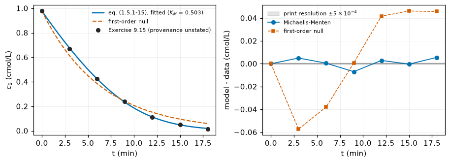

Fit, not test: r_m and K_M were fitted to these same seven points. The residual band shows why the table cannot be an exactly-rounded model evaluation - it is 13.9x too wide for that.

2. The Lineweaver construction, run exactly as both books instruct

Froment says to plot \(1/r\) against \(C_{\rm A}\); Levenspiel p. 615 says \(1/(-r_{\rm A})\) against \(1/C_{\rm A}\). The first cell settles which is right from Froment’s own eq. (1.5.1-15) - by measuring, on the fitted constants, how far each is from a straight line. The second runs the exercise’s hint on the actual table (rates by central difference, then unweighted linear least squares on the reciprocals) and compares what comes out with the direct fit, which is the comparison Levenspiel makes a claim about.

# "How far from a straight line" is a MAXIMUM OVER AN INTERVAL, and it is only
# well posed once WHICH straight line is named. Three answers are computed here,
# and the difference between them is larger than any grid effect:
#   (i) the CHEBYSHEV (minimax) line is the one that minimises this very
#       statistic, so it is the FLOOR - the honest answer to "how close can a
#       straight line get". It needs no weighting convention at all, and for a
#       convex A/C + B it is closed form with an equioscillation certificate.
#   (ii) a LEAST-SQUARES line minimises a different (square) norm, so it is
#       always further away in the max norm, and it additionally depends on how
#       the interval is WEIGHTED: a least-squares fit on a geomspace grid
#       weights it as dC/C, on a linspace grid as dC. Those two give 0.503 and
#       0.669; the page reports both and names the one it quotes.
#   (iii) in every case the maximum is ROOT-FOUND, not sampled: with the line
#       fixed, the deviation of A/C + B from q0 + q1 C has one interior
#       stationary point, C* = sqrt(-A/q1), in closed form.
# Moments and extrema are therefore all exact - there is no grid under any of
# these numbers. The grid sequence below is shown only as evidence that refining
# a 400-point grid converges to the closed form.
A_LW, B_LW = KM_fit/rm_fit, 1.0/rm_fit             # 1/r = A/C_A + B


def straightness_exact(a, b, weight="log", line=False):
    """max |1/r - best LEAST-SQUARES line in C_A| / range, on [a, b].

    Least squares minimises a square norm, NOT the maximum reported here, so
    this is an upper bound on the distance from the best straight line, never
    the distance itself - straightness_minimax gives that.
    `weight` = 'log' (dC/C, the geomspace convention) or 'uniform' (dC).
    `line=True` returns the line's (intercept, slope) instead, so that the
    figure can draw the same line the number is measured against.
    Closed-form weighted least squares, root-found extremum.
    """
    L = np.log(b/a)
    if weight == "log":
        m0, m1, m2 = L, b - a, (b*b - a*a)/2
        n0, n1 = A_LW*(1/a - 1/b) + B_LW*L, A_LW*L + B_LW*(b - a)
    else:
        m0, m1, m2 = b - a, (b*b - a*a)/2, (b**3 - a**3)/3
        n0, n1 = A_LW*L + B_LW*(b - a), A_LW*(b - a) + B_LW*(b*b - a*a)/2
    q0, q1 = np.linalg.solve(np.array([[m0, m1], [m1, m2]]), np.array([n0, n1]))
    if line:
        return float(q0), float(q1)
    dev = lambda x: A_LW/x + B_LW - q0 - q1*x
    xs = [a, b]
    xc = np.sqrt(-A_LW/q1) if q1 < 0 else None     # dev'(x) = -A/x^2 - q1 = 0
    if xc is not None and a < xc < b:
        xs.append(float(xc))
    return float(max(abs(dev(x)) for x in xs)/(A_LW*(1/a - 1/b)))


def dev_sup(q0, q1, a, b):
    """sup |1/r - (q0 + q1 C)| on [a, b], EXACTLY - no grid.

    1/r - line is convex in C, so its extrema on the interval are the two
    endpoints and the single interior stationary point sqrt(-A/q1).
    """
    d = lambda x: A_LW/x + B_LW - q0 - q1*x
    xs = [a, b]
    if q1 < 0 and a < np.sqrt(-A_LW/q1) < b:
        xs.append(float(np.sqrt(-A_LW/q1)))
    return max(abs(d(x)) for x in xs)


def straightness_minimax(a, b):
    """max |1/r - THE BEST STRAIGHT LINE in C_A| / range, on [a, b].

    Best in the CHEBYSHEV (minimax) sense: the line that minimises the maximum
    deviation, i.e. the statistic actually being reported. No straight line does
    better, so this is a convention-free FLOOR - it needs no weighting, and the
    normalisation by the range cancels r_m and K_M exactly, leaving a pure
    property of the interval.

    Closed form for a strictly convex f = A/C + B: the optimal slope is the
    chord slope m = (f(b)-f(a))/(b-a), the tangency is at sqrt(A/|m|) = sqrt(ab),
    and the deviation equioscillates + - + at a, sqrt(ab), b. Chebyshev's
    theorem makes that equioscillation an optimality CERTIFICATE - but by
    CONSTRUCTION here, not by an independent check: q0 is set to the midpoint
    of g(a) and g(xt), so d[0] = -d[1] identically, and m is the exact chord
    slope, so g(b) = g(a) and d[2] = d[0] identically. The equal-magnitude
    assert below therefore compares each of those to itself up to round-off;
    what it actually earns is a < xt < b (tangency interior) and d[0] > 0
    (convexity, i.e. xt is a minimum of g, not a maximum). The 21x21
    perturbation scan two cells down is the part of this notebook that tests
    optimality from outside the construction.
    """
    f = lambda x: A_LW/x + B_LW
    m = (f(b) - f(a))/(b - a)                       # chord slope
    xt = float(np.sqrt(A_LW/abs(m)))                # = sqrt(ab); f'(xt) = m
    assert a < xt < b, (a, xt, b)
    g = lambda x: f(x) - m*x
    q0 = (g(a) + g(xt))/2                           # line midway between them
    d = [g(a) - q0, g(xt) - q0, g(b) - q0]
    assert d[0] > 0 > d[1] and d[2] > 0, d          # alternating signs, + - +
    assert max(abs(abs(v) - abs(d[0])) for v in d) < 1e-12*abs(d[0]), d
    return float(abs(d[0])/(A_LW*(1/a - 1/b)))


def straightness(x, y):
    """The sampled version: max |y - lstsq line in x| / range(y) on a grid."""
    A = np.vstack([x, np.ones_like(x)]).T
    b = np.linalg.lstsq(A, y, rcond=None)[0]
    return float(np.max(np.abs(y - A@b))/np.ptp(y))


LW_A, LW_B = 0.05, 1.0                              # spans the data's own range
c_ex = np.geomspace(LW_A, LW_B, 400)
r_ex = rm_fit*c_ex/(KM_fit + c_ex)
M["lineweaver_printed_axes_nonlinearity_minimax"] = straightness_minimax(LW_A, LW_B)
M["lineweaver_printed_axes_nonlinearity"] = straightness_exact(LW_A, LW_B, "log")
M["lineweaver_printed_axes_nonlinearity_uniform_measure"] = \
    straightness_exact(LW_A, LW_B, "uniform")
M["lineweaver_correct_axes_nonlinearity"] = straightness(1/c_ex, 1/r_ex)
print(f"exact eq. (1.5.1-15) on {LW_A}-{LW_B} cmol/L, distance from a straight "
      f"line,\nas a fraction of the range of 1/r over that interval. WHICH "
      f"straight line is\npart of the question, and it is the bigger lever of "
      f"the two conventions here:")
print(f"  1/r vs C_A, MINIMAX line -- THE best straight line   : "
      f"{M['lineweaver_printed_axes_nonlinearity_minimax']:.6f}"
      f"   <- floor, no convention")
print(f"  1/r vs C_A, best LEAST-SQUARES line, log-weighted    : "
      f"{M['lineweaver_printed_axes_nonlinearity']:.6f}   <- the page's quoted "
      f"convention")
print(f"  1/r vs C_A, best LEAST-SQUARES line, uniform         : "
      f"{M['lineweaver_printed_axes_nonlinearity_uniform_measure']:.6f}")
print(f"  1/r vs 1/C_A (Levenspiel p. 615), least squares      : "
      f"below 1e-13 (here {M['lineweaver_correct_axes_nonlinearity']:.1e})")
print(f"  and symbolically d2(1/r)/dC_A^2 = {CURV} > 0, so no straight line "
      f"exists\n  -- which is the convention-free part, and the part the defect "
      f"rests on.")
print(f"\n  THE STATISTIC IS A MAXIMUM, so the line that minimises it is the "
      f"CHEBYSHEV\n  line, not a least-squares one: a straight line does come "
      f"within "
      f"{100*M['lineweaver_printed_axes_nonlinearity_minimax']:.1f} % of the\n"
      f"  range, and the two least-squares numbers "
      f"({100*M['lineweaver_printed_axes_nonlinearity']:.1f} % and "
      f"{100*M['lineweaver_printed_axes_nonlinearity_uniform_measure']:.1f} %) "
      f"answer a\n  different question and do not even bracket it.")
_mmx = M["lineweaver_printed_axes_nonlinearity_minimax"]
_f = lambda x: A_LW/x + B_LW
_m = (_f(LW_B) - _f(LW_A))/(LW_B - LW_A)
_g = lambda x: _f(x) - _m*x
_q0 = (_g(LW_A) + _g(float(np.sqrt(A_LW/abs(_m)))))/2
_rng = A_LW*(1/LW_A - 1/LW_B)
_PN, _PD = 21, 0.05
_pert = [dev_sup(_q0*(1 + du), _m*(1 + dv), LW_A, LW_B)/_rng
         for du in np.linspace(-_PD, _PD, _PN)
         for dv in np.linspace(-_PD, _PD, _PN) if du or dv]
_worst = min(_pert)
assert _worst > _mmx, (_worst, _mmx)
print(f"  the three deviations at C = {LW_A:g}, {np.sqrt(LW_A*LW_B):.7f}, "
      f"{LW_B:g} are equal in size and\n  alternate in sign (asserted), which is "
      f"Chebyshev's optimality certificate; and no\n  perturbed line in a "
      f"{_PN} x {_PN} grid of +-{100*_PD:g} % on its slope and intercept beats "
      f"it -\n  the best of those {len(_pert)} gets to {_worst:.6f} against the "
      f"floor's {_mmx:.6f}.")
print("\n  the two LEAST-SQUARES conventions are LIMITS of the two obvious "
      "grids, and the\n  grid the page originally used (geomspace, n = 400) was "
      "not converged at four digits:")
for n in (400, 1600, 6400, 25600):
    cg, cl = np.geomspace(LW_A, LW_B, n), np.linspace(LW_A, LW_B, n)
    print(f"    n = {n:6d}   geomspace {straightness(cg, (KM_fit+cg)/(rm_fit*cg)):.6f}"
          f"   linspace {straightness(cl, (KM_fit+cl)/(rm_fit*cl)):.6f}")
print(f"    n -> inf     geomspace {M['lineweaver_printed_axes_nonlinearity']:.6f}"
      f"   linspace "
      f"{M['lineweaver_printed_axes_nonlinearity_uniform_measure']:.6f}"
      f"   (closed form)")


def lineweaver(tv, yv):
    """The exercise's hint: central-difference rates, then LS on 1/r vs 1/c."""
    cm = 0.5*(yv[:-1] + yv[1:])
    rr = -(yv[1:] - yv[:-1])/(tv[1:] - tv[:-1])
    A = np.vstack([1/cm, np.ones_like(cm)]).T
    sl, ic = np.linalg.lstsq(A, 1/rr, rcond=None)[0]
    return 1/sl, ic/sl, cm, rr                       # k = 1/slope, K = intercept*k


k_lb, K_lb, cm_d, r_d = lineweaver(t_d, c_d)
k_lbm, K_lbm, _, _ = lineweaver(t_d, s_closed(t_d, cA0, rm_fit, KM_fit))
M["lb_rm_bias_vs_nls"] = (k_lb/K_lb)/rm_fit - 1
M["lb_KM_bias_vs_nls"] = (1/K_lb)/KM_fit - 1
M["lb_KM_bias_finite_difference_only"] = (1/K_lbm)/KM_fit - 1
print(f"\nLineweaver on the seven printed points : k = {k_lb:.5f}, K = {K_lb:.5f}")
print(f"   -> r_m = {k_lb/K_lb:.5f} ({100*M['lb_rm_bias_vs_nls']:+.2f} %), "
      f"K_M = {1/K_lb:.5f} ({100*M['lb_KM_bias_vs_nls']:+.2f} %) vs the direct fit")
print(f"same construction on the FITTED CURVE sampled at the same seven times : "
      f"K_M = {1/K_lbm:.5f} ({100*M['lb_KM_bias_finite_difference_only']:+.2f} %)")
print("   so the differencing alone biases K_M UP by 14 %; the rest of the -47 %"
      " is the reciprocal transform amplifying the scatter of the last points.")
print("   Levenspiel p. 615 says the direct C_A-versus-tau fit 'is direct, is "
      "less prone to fiddling, and is more reliable'. On this dataset it is.")

exact eq. (1.5.1-15) on 0.05-1.0 cmol/L, distance from a straight line,
as a fraction of the range of 1/r over that interval. WHICH straight line is
part of the question, and it is the bigger lever of the two conventions here:
  1/r vs C_A, MINIMAX line -- THE best straight line   : 0.317256   <- floor, no convention
  1/r vs C_A, best LEAST-SQUARES line, log-weighted    : 0.503158   <- the page's quoted convention
  1/r vs C_A, best LEAST-SQUARES line, uniform         : 0.668756
  1/r vs 1/C_A (Levenspiel p. 615), least squares      : below 1e-13 (here 4.8e-16)
  and symbolically d2(1/r)/dC_A^2 = 2*K_M/(C_A**3*r_m) > 0, so no straight line exists
  -- which is the convention-free part, and the part the defect rests on.

  THE STATISTIC IS A MAXIMUM, so the line that minimises it is the CHEBYSHEV
  line, not a least-squares one: a straight line does come within 31.7 % of the
  range, and the two least-squares numbers (50.3 % and 66.9 %) answer a
  different question and do not even bracket it.
  the three deviations at C = 0.05, 0.2236068, 1 are equal in size and
  alternate in sign (asserted), which is Chebyshev's optimality certificate; and no
  perturbed line in a 21 x 21 grid of +-5 % on its slope and intercept beats it -
  the best of those 440 gets to 0.318434 against the floor's 0.317256.

  the two LEAST-SQUARES conventions are LIMITS of the two obvious grids, and the
  grid the page originally used (geomspace, n = 400) was not converged at four digits:
    n =    400   geomspace 0.502442   linspace 0.665642
    n =   1600   geomspace 0.502980   linspace 0.667984
    n =   6400   geomspace 0.503114   linspace 0.668563
    n =  25600   geomspace 0.503147   linspace 0.668708
    n -> inf     geomspace 0.503158   linspace 0.668756   (closed form)

Lineweaver on the seven printed points : k = 0.40003, K = 3.73157
   -> r_m = 0.10720 (-34.06 %), K_M = 0.26798 (-46.73 %) vs the direct fit
same construction on the FITTED CURVE sampled at the same seven times : K_M = 0.57361 (+14.02 %)
   so the differencing alone biases K_M UP by 14 %; the rest of the -47 % is the reciprocal transform amplifying the scatter of the last points.
   Levenspiel p. 615 says the direct C_A-versus-tau fit 'is direct, is less prone to fiddling, and is more reliable'. On this dataset it is.

fig, ax = plt.subplots(1, 2, figsize=(8.4, 3.1))
# plotted over the data's own range; the METRICS above are read on 0.05-1.0,
# which is a stated choice and has its own break row
c_pl = np.geomspace(0.9*cm_d.min(), 1.0, 400)
r_pl = rm_fit*c_pl/(KM_fit + c_pl)
ax[0].plot(1/c_pl, 1/r_pl, color=C_BLUE, lw=1.6, label="eq. (1.5.1-15), exact")
A = np.vstack([1/c_pl, np.ones_like(c_pl)]).T
ax[0].plot(1/c_pl, A@np.linalg.lstsq(A, 1/r_pl, rcond=None)[0], color=C_GREY,
           lw=0.9, ls=":", label="straight line")
ax[0].plot(1/cm_d, 1/r_d, "o", ms=5, color="0.15", label="Exercise 9.15, differenced")
ax[0].set_xlabel(r"$1/C_{\rm A}$ (L/cmol)")
ax[0].set_ylabel(r"$1/r$ (L min/cmol)")
ax[0].set_title("Levenspiel p. 615 axes: exactly straight", fontsize=9)
ax[0].legend(fontsize=7.5, frameon=False); ax[0].grid(alpha=0.25, lw=0.5)

ax[1].plot(c_pl, 1/r_pl, color=C_ORANGE, lw=1.6, label="eq. (1.5.1-15), exact")
# BOTH lines are the ones fitted on 0.05-1.0 cmol/L - the interval the two
# reported percentages are measured on - drawn across the data's own range.
# The dotted one minimises a log-weighted SQUARE error (50.3 %); the dashed one
# minimises the MAXIMUM deviation, which is the statistic being reported, and is
# therefore the best straight line there is (31.7 %).
_qls = straightness_exact(LW_A, LW_B, "log", line=True)
ax[1].plot(c_pl, _qls[0] + _qls[1]*c_pl, color=C_GREY,
           lw=0.9, ls=":", label="best least-squares line")
ax[1].plot(c_pl, _q0 + _m*c_pl, color="0.35", lw=0.9, ls="--",
           label="best straight line (minimax)")
ax[1].plot(cm_d, 1/r_d, "o", ms=5, color="0.15", label="Exercise 9.15, differenced")
ax[1].set_xlabel(r"$C_{\rm A}$ (cmol/L)")
ax[1].set_ylabel(r"$1/r$ (L min/cmol)")
ax[1].set_title(f"Froment p. 25 axes, 0.05-1.0 cmol/L: no straight line "
                f"closer than "
                f"{100*M['lineweaver_printed_axes_nonlinearity_minimax']:.1f}"
                f" % of range", fontsize=9)
ax[1].legend(fontsize=7.5, frameon=False); ax[1].grid(alpha=0.25, lw=0.5)
fig.tight_layout(); plt.show()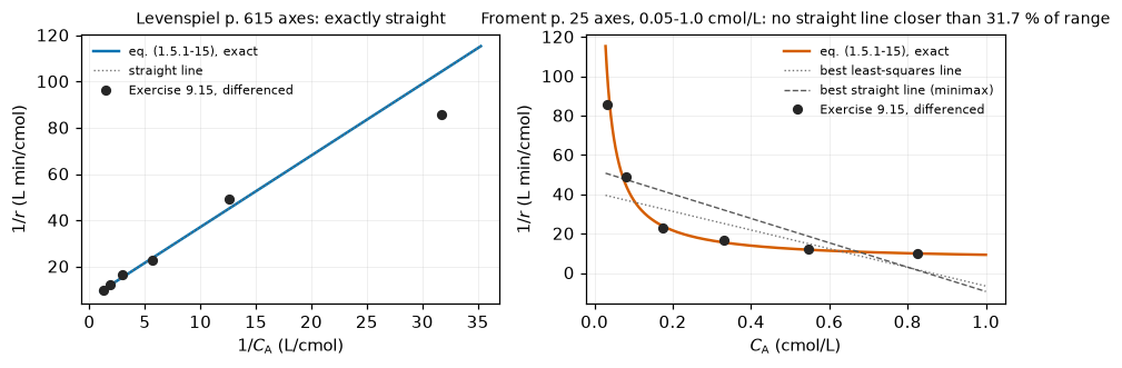

3. The degeneracy: what a steady-state rate measurement cannot see

This is the case’s own question, and it was already settled symbolically in the symbolic cell under The published model: under the reparameterisation, eq. (1.5.1-13) is eq. (1.5.1-15) and \(\partial r/\partial \rho \equiv 0\). What follows is the numerical check on that algebra, not the evidence for it. Hold the two observable constants \((r_m, K_M)\) fixed, sweep \(\rho = k_2/k_{-1}\) over eight decades, and evaluate the rate law from the elementary constants on a four-decade concentration grid. If the two derivations were separable by rate-versus-substrate data, the curves would move.

The check returns exactly zero, and the cell then says what that zero is worth: it needs two floating-point round trips to be exact, and over 2000 random \((\rho, C_{\rm E}^0)\) draws they are not, so the same computation returns ulp-level noise instead. Both numbers are reported.

rho_dec = np.geomspace(1e-4, 1e4, 9)
cg = np.geomspace(1e-3, 10.0, 400)
base = rm_fit*cg/(KM_fit + cg)
CE0_probe = 1e-3

worst = 0.0
rows = []
for r_ in rho_dec:
    kf, kr, kc = elem(r_, CE0_probe, rm_fit, KM_fit)
    r_from_elem = kc*CE0_probe*cg/((kr + kc)/kf + cg)      # (1.5.1-13)+(1.5.1-14)
    d = float(np.max(np.abs(r_from_elem/base - 1)))
    worst = max(worst, d)
    rows.append((r_, kf, kr, kc, kr/kf, d))
M["rate_law_rho_degeneracy_max_rel"] = worst
M["KM_ratio_at_rho_1e4"] = 1.0 + 1e4

# The exact 0.0 above is a property of these nine rho at this C_E0: it needs the
# float round trips (k_-1+k_2)/k_1 == K_M and k_2 C_E0 == r_m to be exact, and
# they are here. Over random draws they are not, and the same computation returns
# ULP-level noise instead. THE ALGEBRA IS THE RESULT (proved in the first cell);
# this is the size of the arithmetic underneath it.
_rng = np.random.default_rng(20260813)             # seeded: determinism
_worst_rand, _inexact, _NDRAW = 0.0, 0, 2000
for _ in range(_NDRAW):
    r_, ce_ = 10**_rng.uniform(-4, 4), 10**_rng.uniform(-5, -1)
    kf, kr, kc = elem(r_, ce_, rm_fit, KM_fit)
    _worst_rand = max(_worst_rand, float(np.max(np.abs(
        kc*ce_*cg/((kr + kc)/kf + cg)/base - 1))))
    _inexact += not ((kr + kc)/kf == KM_fit and kc*ce_ == rm_fit)
M["rate_law_rho_degeneracy_random_draws_max_rel"] = _worst_rand

df = pd.DataFrame(rows, columns=["rho = k2/k-1", "k1 (L/cmol/min)", "k-1 (1/min)",
                                 "k2 (1/min)", "K_M(MM) = k-1/k1", "max |dr/r|"])
show(df.style.format({"rho = k2/k-1": "{:.0e}", "k1 (L/cmol/min)": "{:.4g}",
                      "k-1 (1/min)": "{:.4g}", "k2 (1/min)": "{:.4g}",
                      "K_M(MM) = k-1/k1": "{:.6f}", "max |dr/r|": "{:.2e}"})
     .set_caption("All nine mechanisms have r_m = %.6f and K_M(BH) = %.6f"
                  % (rm_fit, KM_fit)).set_uuid("j46deg"))
print(f"max relative difference in r(C_A) across eight decades of rho: below 1e-14 "
      f"(here {worst:.1e})")
print(f"K_M(Briggs-Haldane)/K_M(Michaelis-Menten) = 1 + rho over the same sweep: "
      f"{1+rho_dec[0]:.5f} .. {1+rho_dec[-1]:.4g}")
print()
print("WHAT THAT EXACT ZERO IS, AND IS NOT. The degeneracy is proved above in "
      "sympy;\nthe 0.0 here additionally requires the float round trips "
      "(k_-1+k_2)/k_1 == K_M and\nk_2 C_E0 == r_m to be exact, which they happen "
      f"to be for these nine rho at\nC_E0 = {CE0_probe:g}. Over {_NDRAW} random "
      f"(rho, C_E0) draws from the same ranges they are\ninexact in {_inexact} "
      f"cases, and the same computation returns below 1e-14 (here up to "
      f"{M['rate_law_rho_degeneracy_random_draws_max_rel']:.1e})\n-- a few ulp of "
      "the rate, not a failure of the identity. Reported as such.")
print()
print("Companion that CAN move (the break table uses it): raise k2 by 1 % and "
      "leave C_E0 alone, so r_m is no longer held fixed --")
kf, kr, kc = elem(1.0, CE0_probe, rm_fit, KM_fit)
kc2 = 1.01*kc
M["rate_law_break_k2_plus_1pct"] = float(np.max(np.abs(
    kc2*CE0_probe*cg/((kr + kc2)/kf + cg)/base - 1)))
print(f"   max |dr/r| = {M['rate_law_break_k2_plus_1pct']:.4e}")

Table 1: All nine mechanisms have r_m = 0.162583 and K_M(BH) = 0.503055

	rho = k2/k-1	k1 (L/cmol/min)	k-1 (1/min)	k2 (1/min)	K_M(MM) = k-1/k1	max |dr/r|
0	1e-04	3.232e+06	1.626e+06	162.6	0.503005	0.00e+00
1	1e-03	3.235e+05	1.626e+05	162.6	0.502553	0.00e+00
2	1e-02	3.264e+04	1.626e+04	162.6	0.498074	0.00e+00
3	1e-01	3555	1626	162.6	0.457323	0.00e+00
4	1e+00	646.4	162.6	162.6	0.251528	0.00e+00
5	1e+01	355.5	16.26	162.6	0.045732	0.00e+00
6	1e+02	326.4	1.626	162.6	0.004981	0.00e+00
7	1e+03	323.5	0.1626	162.6	0.000503	0.00e+00
8	1e+04	323.2	0.01626	162.6	0.000050	0.00e+00

max relative difference in r(C_A) across eight decades of rho: below 1e-14 (here 0.0e+00)
K_M(Briggs-Haldane)/K_M(Michaelis-Menten) = 1 + rho over the same sweep: 1.00010 .. 1e+04

WHAT THAT EXACT ZERO IS, AND IS NOT. The degeneracy is proved above in sympy;
the 0.0 here additionally requires the float round trips (k_-1+k_2)/k_1 == K_M and
k_2 C_E0 == r_m to be exact, which they happen to be for these nine rho at
C_E0 = 0.001. Over 2000 random (rho, C_E0) draws from the same ranges they are
inexact in 87 cases, and the same computation returns below 1e-14 (here up to 4.4e-16)
-- a few ulp of the rate, not a failure of the identity. Reported as such.

Companion that CAN move (the break table uses it): raise k2 by 1 % and leave C_E0 alone, so r_m is no longer held fixed --
   max |dr/r| = 9.7582e-03

4. What a batch transient sees, and at what order

The rate law is blind to \(\rho\); the full mass-action solution is not, because the quasi-steady-state approximation that produced the rate law is itself only approximate, and the size of its error depends on \(\rho\). So the signal a batch run carries about \(\rho\) is the same size as the error in the model that made the question sensible.

Three measurements, and the order matters. (a) Over the whole run, where the maximum turns out to sit inside the induction layer - which is why it is root-found on a logarithmic scan and not read off a uniform one; the uniform scan is 66 % low. (b) Over the window an experiment sampled like the printed table can see, \(t \ge 3\) min, where only about a quarter of that survives as a persistent offset. (c) The honest version of (b): the same question with \(r_m\), \(K_M\) and \(C_{\rm E}^0\) all free to compensate, which is what a fit would do.

(c) is not measured the way (b) is, and the page does not pretend otherwise. (b) is a maximum over \(t\) of the spread between two curves; (c) is an RMS over a 25-point grid starting at \(t = 0\) of a refitted misfit. Dividing (c) by (b) therefore charges to compensation a factor that is partly just the change of statistic and window. The second cell below measures the missing third quantity - the same RMS on the same grid with nothing free - so that the price of compensation can be quoted like for like.

te = np.linspace(0, 18, 181)
red = s_closed(te, cA0, rm_fit, KM_fit)


RHO_LO, RHO_HI = 1e-4, 1e4
eps_of = lambda CE0: CE0/(cA0 + KM_fit)


def ca_of_rho(rho, CE0):
    return mass_action(elem(rho, CE0, rm_fit, KM_fit), CE0, te, dense=True)


T_OBS = float(t_d[1])          # 3 min: the earliest time the printed table samples
WIN_ALL, WIN_OBS = (0.0, 18.0), (T_OBS, 18.0)


def rho_spread(CE0, lo=RHO_LO, hi=RHO_HI, window=WIN_OBS, check=False, with_t=False):
    """max |C_A(t; rho_lo) - C_A(t; rho_hi)| over `window`, ROOT-FOUND in t.

    check=True verifies on a 9-point rho grid that the ENDPOINTS really are the
    extremes, i.e. that the full-grid spread equals the endpoint spread. C_A(t)
    is NOT monotone in rho at every t - the curves cross late in the run, when
    they are all near zero - so this is checked rather than assumed.
    """
    if check:
        tw = np.linspace(*window, 181)
        Y = np.array([mass_action(elem(r_, CE0, rm_fit, KM_fit), CE0, tw)
                      for r_ in np.geomspace(lo, hi, 9)])
        full, ends = float(np.max(Y.max(0) - Y.min(0))), float(np.max(np.abs(Y[0] - Y[-1])))
        assert abs(full - ends) <= 1e-12 + 1e-9*full, (CE0, full, ends)
    return max_gap(ca_of_rho(lo, CE0), ca_of_rho(hi, CE0), window=window, with_t=with_t)


# (a) over the whole run, where the maximum sits INSIDE THE INDUCTION LAYER
v_all, t_all = rho_spread(1e-4, window=WIN_ALL, with_t=True)
M["rho_spread_induction_over_eps"] = v_all/eps_of(1e-4)
M["rho_spread_induction_peak_min"] = t_all
print(f"over the whole run at C_E0 = 1e-4: spread = {v_all:.6e} cmol/L "
      f"(= {v_all/eps_of(1e-4):.4f} eps), attained at t = {t_all:.3e} min")
sc_unif = float(np.max(np.abs(ca_of_rho(RHO_LO, 1e-4)(te) - ca_of_rho(RHO_HI, 1e-4)(te))))
M["sampled_max_shortfall_uniform_scan"] = 1.0 - sc_unif/v_all
print(f"  a UNIFORM 181-point scan of the same window reads {sc_unif:.6e}, "
      f"{100*M['sampled_max_shortfall_uniform_scan']:.1f} % low -- the whole "
      f"signal is in the first ~1e-3 min")
print(f"  induction timescale 1/(k1(c_A0+K_M)): "
      f"{1/(elem(RHO_LO,1e-4,rm_fit,KM_fit)[0]*(cA0+KM_fit)):.2e} min at rho = 1e-4, "
      f"{1/(elem(RHO_HI,1e-4,rm_fit,KM_fit)[0]*(cA0+KM_fit)):.2e} min at rho = 1e4")
print("  THIS IS INVISIBLE TO THE PRINTED TABLE, whose first sample after t = 0 "
      f"is at {T_OBS:g} min. It is what Froment p. 25 means by 'only transient\n"
      "  experimentation (stopped flow, or relaxation ...) can help'.")

# (b) over the window an experiment sampling like the printed table can see
SPREAD = {CE0: rho_spread(CE0, check=True) for CE0 in (1e-4, 1e-3, 1e-2, 1e-1)}
M["rho_spread_over_eps_trace_limit"] = SPREAD[1e-4]/eps_of(1e-4)
print(f"\nover the OBSERVABLE window t in [{T_OBS:g}, 18] min "
      f"(9-point rho grid confirms the endpoints are the extremes):")
for CE0, v in SPREAD.items():
    print(f"  C_E0 = {CE0:7.0e} cmol/L   eps = {eps_of(CE0):.4e}   "
          f"spread = {v:.6e} cmol/L   spread/eps = {v/eps_of(CE0):.4f}")

CE0_star = 10**brentq(lambda g: rho_spread(10**g) - RES, -4, 0, xtol=1e-8)
rho_spread(CE0_star, check=True)              # the endpoint check, at the root too
M["CE0_star_cmol_per_L"] = CE0_star
M["eps_star_rho_visible_at_print_resolution"] = eps_of(CE0_star)
print(f"\nROOT-FOUND in BOTH coordinates (the peak in t, then the threshold in "
      f"C_E0):\n  the observable spread reaches the {RES:g} cmol/L print "
      f"resolution at C_E0 = {CE0_star:.6e} cmol/L,\n  i.e. eps = "
      f"{eps_of(CE0_star):.6e}")
print("  -- and this holds r_m, K_M and C_E0 fixed, which no real fit does.")

over the whole run at C_E0 = 1e-4: spread = 6.598393e-05 cmol/L (= 0.9773 eps), attained at t = 2.011e-07 min
  a UNIFORM 181-point scan of the same window reads 2.225547e-05, 66.3 % low -- the whole signal is in the first ~1e-3 min
  induction timescale 1/(k1(c_A0+K_M)): 2.09e-08 min at rho = 1e-4, 2.09e-04 min at rho = 1e4
  THIS IS INVISIBLE TO THE PRINTED TABLE, whose first sample after t = 0 is at 3 min. It is what Froment p. 25 means by 'only transient
  experimentation (stopped flow, or relaxation ...) can help'.

over the OBSERVABLE window t in [3, 18] min (9-point rho grid confirms the endpoints are the extremes):
  C_E0 =   1e-04 cmol/L   eps = 6.7519e-05   spread = 1.635811e-05 cmol/L   spread/eps = 0.2423
  C_E0 =   1e-03 cmol/L   eps = 6.7519e-04   spread = 1.634577e-04 cmol/L   spread/eps = 0.2421
  C_E0 =   1e-02 cmol/L   eps = 6.7519e-03   spread = 1.622230e-03 cmol/L   spread/eps = 0.2403
  C_E0 =   1e-01 cmol/L   eps = 6.7519e-02   spread = 1.500097e-02 cmol/L   spread/eps = 0.2222

ROOT-FOUND in BOTH coordinates (the peak in t, then the threshold in C_E0):
  the observable spread reaches the 0.0005 cmol/L print resolution at C_E0 = 3.064199e-03 cmol/L,
  i.e. eps = 2.068930e-03
  -- and this holds r_m, K_M and C_E0 fixed, which no real fit does.

# --- the honest version: can a fit at the WRONG rho reproduce the data?
tt_d = np.linspace(0, 18, 25)


def discriminate(eps, rho_true=1e4, rho_fit=1e-4, grid=None,
                 rtol=1e-11, atol=1e-14):
    """Min RMS misfit of the rho_fit model to noise-free rho_true data,
    with r_m, K_M and C_E0 all free. An optimiser returns an UPPER BOUND on a
    minimum, so 'not separable' is the safe direction.

    rtol/atol are exposed so that a break row can loosen the ODE solve UNDERNEATH
    the root-find - a perturbation of the computation rather than of a declared
    convention, which is the only kind that can expose a wrong baseline."""
    grid = tt_d if grid is None else grid
    CE0 = eps*(cA0 + KM_fit)
    truth = mass_action(elem(rho_true, CE0, rm_fit, KM_fit), CE0, grid,
                        rtol=rtol, atol=atol)

    def rr(q):
        rmv, KMv, CE0v = np.exp(q)
        return mass_action(elem(rho_fit, CE0v, rmv, KMv), CE0v, grid,
                           rtol=rtol, atol=atol) - truth

    best = None
    for g in ([rm_fit, KM_fit, CE0], [1.2*rm_fit, 0.8*KM_fit, 0.5*CE0]):
        r = least_squares(rr, np.log(g), xtol=1e-13, ftol=1e-13, gtol=1e-13)
        if best is None or r.cost < best.cost:
            best = r
    return float(np.sqrt(np.mean(best.fun**2))), np.exp(best.x)


print("misfit of a rho = 1e-4 model to rho = 1e4 data, everything else free:")
for eps in (1e-3, 1e-2, 3e-2, 1e-1):
    v, q = discriminate(eps)
    print(f"  eps = {eps:.0e}  RMS = {v:.4e} cmol/L   "
          f"(refitted r_m {q[0]:.5f}, K_M {q[1]:.5f}, C_E0 {q[2]:.4e})")
rev = discriminate(1e-1, rho_true=1e-4, rho_fit=1e4)[0]
print(f"  reverse direction at eps = 1e-1: {rev:.4e} -- larger, so the direction "
      f"reported is the binding one")

# EVERY brentq on this threshold uses this one tolerance, in log10(eps). It is
# named rather than repeated so that the break table can DERIVE the resolution of
# a difference between two such root-finds instead of choosing a round number for
# it: ln(10)*XTOL_LOG10 relative per root-find, twice that for a difference.
XTOL_LOG10 = 1e-6
eps_star_c = 10**brentq(lambda g: discriminate(10**g)[0] - RES, -2, np.log10(0.2),
                        xtol=XTOL_LOG10)
M["eps_star_discrimination_with_compensation"] = eps_star_c
print(f"\nROOT-FOUND: with the other three constants free, telling rho = 1e-4 from "
      f"rho = 1e4\n  at the {RES:g} cmol/L resolution needs eps = {eps_star_c:.6e}"
      f"  (C_E0 = {eps_star_c*(cA0+KM_fit):.6e} cmol/L,\n  brentq at xtol = "
      f"{XTOL_LOG10:g} in log10, i.e. {np.log(10)*XTOL_LOG10:.2e} relative).")

# ---- LIKE FOR LIKE. eps_star_rho_visible_at_print_resolution is a MAX over
# t in [3, 18] of the rho-spread; eps_star_discrimination_with_compensation is an
# RMS over tt_d (25 points, from t = 0) of a REFITTED misfit. Dividing one by the
# other charges the whole ratio to compensation, which is wrong: part of it is
# the change of statistic and window. So the SAME statistic on the SAME grid is
# measured here with rho pinned and NOTHING free, and that is the baseline the
# compensation penalty is quoted against.
def spread_rms_same_grid(eps, lo=RHO_LO, hi=RHO_HI):
    """RMS over tt_d of |C_A(rho=lo) - C_A(rho=hi)|; r_m, K_M, C_E0 all pinned."""
    CE0 = eps*(cA0 + KM_fit)
    a = mass_action(elem(lo, CE0, rm_fit, KM_fit), CE0, tt_d)
    b = mass_action(elem(hi, CE0, rm_fit, KM_fit), CE0, tt_d)
    return float(np.sqrt(np.mean((a - b)**2)))


eps_star_ll = 10**brentq(lambda g: spread_rms_same_grid(10**g) - RES, -5, 0,
                         xtol=1e-10)
M["eps_star_rms_25pt_grid_no_compensation"] = eps_star_ll
M["eps_star_compensation_penalty"] = eps_star_c/eps_star_ll
M["eps_star_statistic_and_window_factor"] = \
    eps_star_ll/M["eps_star_rho_visible_at_print_resolution"]
M["eps_star_raw_ratio_unlike_statistics"] = \
    eps_star_c/M["eps_star_rho_visible_at_print_resolution"]
print(f"\nTHE THREE EPSILONS, AND WHAT EACH ONE IS. All at the same {RES:g} cmol/L "
      f"resolution\nand the same rho pair [{RHO_LO:g}, {RHO_HI:g}]:")
print(f"  (a) max over t in [{T_OBS:g}, 18] of the spread, nothing free   "
      f"eps* = {M['eps_star_rho_visible_at_print_resolution']:.6e}")
print(f"  (b) RMS over the 25-point grid from t = 0, nothing free  "
      f"eps* = {eps_star_ll:.6e}")
print(f"  (c) the same RMS on the same grid, r_m/K_M/C_E0 free    "
      f"eps* = {eps_star_c:.6e}")
print(f"  (b)/(a) = {M['eps_star_statistic_and_window_factor']:.4f}  <- change of "
      f"STATISTIC and WINDOW only, no compensation")
print(f"  (c)/(b) = {M['eps_star_compensation_penalty']:.4f}  <- THE PRICE OF "
      f"COMPENSATION, like for like")
print(f"  (c)/(a) = {M['eps_star_raw_ratio_unlike_statistics']:.4f}  <- the raw "
      f"ratio of the two headline numbers; it is the product of the two above,\n"
      f"            and quoting it as the cost of compensation overstates that "
      f"cost by "
      f"{M['eps_star_statistic_and_window_factor']:.2f}x")

misfit of a rho = 1e-4 model to rho = 1e4 data, everything else free:
  eps = 1e-03  RMS = 8.4085e-06 cmol/L   (refitted r_m 0.16243, K_M 0.50194, C_E0 1.0202e-03)
  eps = 1e-02  RMS = 8.3019e-05 cmol/L   (refitted r_m 0.16108, K_M 0.49202, C_E0 1.0133e-02)
  eps = 3e-02  RMS = 2.4286e-04 cmol/L   (refitted r_m 0.15810, K_M 0.47049, C_E0 2.9927e-02)
  eps = 1e-01  RMS = 1.3050e-03 cmol/L   (refitted r_m 0.15214, K_M 0.42256, C_E0 9.0107e-02)
  reverse direction at eps = 1e-1: 4.4529e-03 -- larger, so the direction reported is the binding one

ROOT-FOUND: with the other three constants free, telling rho = 1e-4 from rho = 1e4
  at the 0.0005 cmol/L resolution needs eps = 5.797637e-02  (C_E0 = 8.586620e-02 cmol/L,
  brentq at xtol = 1e-06 in log10, i.e. 2.30e-06 relative).

THE THREE EPSILONS, AND WHAT EACH ONE IS. All at the same 0.0005 cmol/L resolution
and the same rho pair [0.0001, 10000]:
  (a) max over t in [3, 18] of the spread, nothing free   eps* = 2.068930e-03
  (b) RMS over the 25-point grid from t = 0, nothing free  eps* = 3.184735e-03
  (c) the same RMS on the same grid, r_m/K_M/C_E0 free    eps* = 5.797637e-02
  (b)/(a) = 1.5393  <- change of STATISTIC and WINDOW only, no compensation
  (c)/(b) = 18.2045  <- THE PRICE OF COMPENSATION, like for like
  (c)/(a) = 28.0224  <- the raw ratio of the two headline numbers; it is the product of the two above,
            and quoting it as the cost of compensation overstates that cost by 1.54x

5. The price of each reduction against the full mass-action solution

Froment states when the pseudo steady state fails (“in particular if the enzyme concentration is relatively large compared to that of the substrate”, p. 25) and states the condition for route 1 only as words (“the decomposition of the complex A-E into the product P and the enzyme E is the rate determining step”). Both are turned into numbers here.

red_f = lambda t: s_closed(t, cA0, rm_fit, KM_fit)
QSSA = {}
for CE0 in (1e-5, 1e-4, 1e-3, 1e-2, 1e-1):
    QSSA[CE0] = {r_: max_gap(ca_of_rho(r_, CE0), red_f)
                 for r_ in (1e-2, 1.0, 1e2)}
ks = sorted(QSSA)
M["qssa_error_order_in_eps"] = float(np.mean(
    [np.log10(QSSA[ks[i]][1.0]/QSSA[ks[i-1]][1.0]) for i in (1, 2, 3)]))
M["qssa_error_over_eps_rho1"] = QSSA[1e-5][1.0]/eps_of(1e-5)
print("max |C_A(full) - C_A(eq. 1.5.1-13)|, cmol/L, divided by eps:")
for CE0 in ks:
    print(f"  C_E0 = {CE0:7.0e}  eps = {eps_of(CE0):.4e}   " +
          "   ".join(f"rho={r_:<6g} {QSSA[CE0][r_]/eps_of(CE0):.4f}"
                     for r_ in (1e-2, 1.0, 1e2)))
print(f"observed order in eps: {M['qssa_error_order_in_eps']:.4f}  "
      f"(first order, as the error being O(eps) requires)")

# the same error evaluated at the enzyme loading a DISCRIMINATING experiment needs
_ce = M["eps_star_discrimination_with_compensation"]*(cA0 + KM_fit)
qssa_at_eps_star = max_gap(ca_of_rho(1.0, _ce), red_f)
M["qssa_error_at_discrimination_eps_over_resolution"] = qssa_at_eps_star/RES
print(f"\nAT eps* = {M['eps_star_discrimination_with_compensation']:.4e}, where "
      f"rho first becomes visible with the other constants free, the pseudo "
      f"steady state\n  is itself off by {qssa_at_eps_star:.5f} cmol/L = "
      f"{M['qssa_error_at_discrimination_eps_over_resolution']:.1f} x the "
      f"{RES:g} resolution the discrimination is read at.")
# WHICH substrate the reduced model is compared against is a convention, and it
# moves this number, so both are printed. The reduced model has one substrate
# variable; the full model has free C_A and bound C_A-E.
qssa_at_eps_star_tot = max_gap(
    mass_action(elem(1.0, _ce, rm_fit, KM_fit), _ce, te, dense=True, total=True),
    red_f)
print(f"  That compares eq. (1.5.1-15) with the FREE substrate C_A. Against the "
      f"TOTAL\n  substrate C_A + C_A-E - the other defensible convention - the "
      f"same error is\n  {qssa_at_eps_star_tot:.5f} cmol/L = "
      f"{qssa_at_eps_star_tot/RES:.1f} x the resolution. Both are far above 1, "
      f"which is the claim;\n  the factor quoted elsewhere on this page is the "
      f"free-C_A one.")

# which group? fix C_E0/c_A0 and sweep K_M over three decades
GROUP = {}
for KMv in (0.05, 0.5, 5.0, 50.0):
    CE0 = 1e-3*cA0
    e = max_gap(mass_action(elem(1.0, CE0, rm_fit, KMv), CE0, te, dense=True),
                lambda t, KMv=KMv: s_closed(t, cA0, rm_fit, KMv))
    GROUP[KMv] = (e, e/1e-3, e/(CE0/(cA0 + KMv)))
M["qssa_group_spread_CE0_over_cA0"] = (max(g[1] for g in GROUP.values())
                                       / min(g[1] for g in GROUP.values()))
M["qssa_group_spread_CE0_over_cA0_plus_KM"] = (max(g[2] for g in GROUP.values())
                                               / min(g[2] for g in GROUP.values()))
print(f"\nat FIXED C_E0/c_A0 = 1e-3, sweeping K_M over three decades:")
for KMv, (e, a, b) in GROUP.items():
    print(f"  K_M = {KMv:6.2f}  error = {e:.4e}   error/(C_E0/c_A0) = {a:.4e}   "
          f"error/(C_E0/(c_A0+K_M)) = {b:.4f}")
print(f"  spread of the ratio: C_E0/c_A0 x{M['qssa_group_spread_CE0_over_cA0']:.1f}, "
      f"C_E0/(c_A0+K_M) x{M['qssa_group_spread_CE0_over_cA0_plus_KM']:.2f}")
print("  Froment's printed comparison is with the substrate alone, which is the "
      "K_M << c_A0 corner of eps and is right there (coefficient 0.95 at "
      "K_M = 0.05); the K_M term is what this page adds.")

max |C_A(full) - C_A(eq. 1.5.1-13)|, cmol/L, divided by eps:
  C_E0 =   1e-05  eps = 6.7519e-06   rho=0.01   0.9747   rho=1      0.8119   rho=100    0.6491
  C_E0 =   1e-04  eps = 6.7519e-05   rho=0.01   0.9747   rho=1      0.8118   rho=100    0.6490
  C_E0 =   1e-03  eps = 6.7519e-04   rho=0.01   0.9745   rho=1      0.8111   rho=100    0.6480
  C_E0 =   1e-02  eps = 6.7519e-03   rho=0.01   0.9723   rho=1      0.8054   rho=100    0.6406
  C_E0 =   1e-01  eps = 6.7519e-02   rho=0.01   0.9505   rho=1      0.7597   rho=100    0.5856
observed order in eps: 0.9988  (first order, as the error being O(eps) requires)

AT eps* = 5.7976e-02, where rho first becomes visible with the other constants free, the pseudo steady state
  is itself off by 0.04443 cmol/L = 88.9 x the 0.0005 resolution the discrimination is read at.
  That compares eq. (1.5.1-15) with the FREE substrate C_A. Against the TOTAL
  substrate C_A + C_A-E - the other defensible convention - the same error is
  0.01939 cmol/L = 38.8 x the resolution. Both are far above 1, which is the claim;
  the factor quoted elsewhere on this page is the free-C_A one.

at FIXED C_E0/c_A0 = 1e-3, sweeping K_M over three decades:
  K_M =   0.05  error = 9.0773e-04   error/(C_E0/c_A0) = 9.0773e-01   error/(C_E0/(c_A0+K_M)) = 0.9541
  K_M =   0.50  error = 5.3717e-04   error/(C_E0/c_A0) = 5.3717e-01   error/(C_E0/(c_A0+K_M)) = 0.8118
  K_M =   5.00  error = 9.2983e-05   error/(C_E0/c_A0) = 9.2983e-02   error/(C_E0/(c_A0+K_M)) = 0.5684
  K_M =  50.00  error = 9.5593e-06   error/(C_E0/c_A0) = 9.5593e-03   error/(C_E0/(c_A0+K_M)) = 0.4983
  spread of the ratio: C_E0/c_A0 x95.0, C_E0/(c_A0+K_M) x1.91
  Froment's printed comparison is with the substrate alone, which is the K_M << c_A0 corner of eps and is right there (coefficient 0.95 at K_M = 0.05); the K_M term is what this page adds.

# --- route 1 (rapid equilibrium, K_M = k_-1/k_1) priced against the full model
CE0t = 1e-5                       # trace enzyme, so the QSSA error is negligible


def eq_route_err(rho, **kw):
    """max_t |C_A(full) - C_A(route 1)|, the maximum ROOT-FOUND in t."""
    p = elem(rho, CE0t, rm_fit, KM_fit)
    return max_gap(mass_action(p, CE0t, te, dense=True, **kw),
                   lambda t: s_closed(t, cA0, rm_fit, p[1]/p[0]))


print("route 1 predicts C_A(t) from the elementary constants via K_M = k_-1/k_1:")
for r_ in (1e-3, 1e-2, 1e-1, 1.0, 10.0):
    p = elem(r_, CE0t, rm_fit, KM_fit)
    print(f"  rho = {r_:8.3g}   K_M(MM) = {p[1]/p[0]:.6f}  "
          f"max |dC_A| = {eq_route_err(r_):.4e}   (route 2: "
          f"{max_gap(mass_action(p, CE0t, te, dense=True), red_f):.4e})")

rho_star = 10**brentq(lambda g: eq_route_err(10**g) - RES, -5, 0, xtol=1e-10)
M["rho_star_equilibrium_route"] = rho_star

# --- SECOND, INDEPENDENT ROUTE to the same number: analytic sensitivity of the
#     closed-form solution to K_M, with the extremum ROOT-FOUND, not sampled.
s_sym, s0_sym, KM_sym = sp.symbols("s s_0 K_M", positive=True)
g_expr = s_sym*sp.log(s0_sym/s_sym)/(s_sym + KM_sym)      # |ds/dK_M| along the curve
g_f = sp.lambdify((s_sym, s0_sym, KM_sym), g_expr, "numpy")
dg_f = sp.lambdify((s_sym, s0_sym, KM_sym), sp.diff(g_expr, s_sym), "numpy")
s_pk = brentq(lambda s: dg_f(s, cA0, KM_fit), 1e-9, cA0*(1 - 1e-12), xtol=1e-14)
gmax = float(g_f(s_pk, cA0, KM_fit))
M["rho_star_equilibrium_analytic"] = RES/(gmax*KM_fit - RES)   # dK_M = K_M rho/(1+rho)
M["rho_star_equilibrium_two_route_rel_diff"] = abs(
    M["rho_star_equilibrium_analytic"]/rho_star - 1)
s_samp = float(np.max(g_f(np.clip(red, 1e-12, None), cA0, KM_fit)))
M["dsdKM_rootfound_over_sampled"] = gmax/s_samp

print(f"\nROOT-FOUND: route 1 reaches the {RES:g} cmol/L resolution at "
      f"rho = k_2/k_-1 = {rho_star:.6e}")
print(f"SECOND ROUTE (analytic sensitivity, no ODE solver, no mass-action model):")
print(f"  ds/dK_M = s ln(s_0/s)/(s + K_M); its maximum is root-found at "
      f"s = {s_pk:.6f}, value {gmax:.6f}")
print(f"  giving rho* = {M['rho_star_equilibrium_analytic']:.6e}, "
      f"{100*M['rho_star_equilibrium_two_route_rel_diff']:.3f} % from the "
      f"nonlinear root-find")
print(f"  (sampling that maximum on the 181-point t grid instead would give "
      f"{s_samp:.6f}, a factor {M['dsdKM_rootfound_over_sampled']:.6f} -- so on "
      f"THIS curve the sample happens to be right, which the root-find is what "
      f"establishes)")

route 1 predicts C_A(t) from the elementary constants via K_M = k_-1/k_1:
  rho =    0.001   K_M(MM) = 0.502553  max |dC_A| = 2.2755e-04   (route 2: 6.6011e-06)
  rho =     0.01   K_M(MM) = 0.498074  max |dC_A| = 2.2689e-03   (route 2: 6.5812e-06)
  rho =      0.1   K_M(MM) = 0.457323  max |dC_A| = 2.1446e-02   (route 2: 6.3995e-06)
  rho =        1   K_M(MM) = 0.251528  max |dC_A| = 1.4009e-01   (route 2: 5.4819e-06)
  rho =       10   K_M(MM) = 0.045732  max |dC_A| = 3.3572e-01   (route 2: 4.5643e-06)

ROOT-FOUND: route 1 reaches the 0.0005 cmol/L resolution at rho = k_2/k_-1 = 2.195118e-03
SECOND ROUTE (analytic sensitivity, no ODE solver, no mass-action model):
  ds/dK_M = s ln(s_0/s)/(s + K_M); its maximum is root-found at s = 0.228461, value 0.454146
  giving rho* = 2.193362e-03, 0.080 % from the nonlinear root-find
  (sampling that maximum on the 181-point t grid instead would give 0.454145, a factor 1.000002 -- so on THIS curve the sample happens to be right, which the root-find is what establishes)

fig, ax = plt.subplots(1, 2, figsize=(8.4, 3.1))
epsv = np.array([eps_of(c) for c in ks])
for r_, col, mk in ((1e-2, C_BLUE, "o"), (1.0, C_ORANGE, "s"), (1e2, C_GREEN, "^")):
    ax[0].loglog(epsv, [QSSA[c][r_] for c in ks], mk + "-", ms=4, lw=1.4, color=col,
                 label=rf"$\rho$ = {r_:g}")
ax[0].loglog(epsv, epsv, ls=":", lw=0.9, color=C_GREY, label=r"slope 1")
ax[0].axhline(RES, color=C_PURPLE, ls="--", lw=1.0)
ax[0].text(epsv[0], RES*1.25, "print resolution", fontsize=7, color=C_PURPLE)
ax[0].set_xlabel(r"$\varepsilon = C_{\rm E}^0/(c_{\rm A0}+K_M)$")
ax[0].set_ylabel(r"max $|C_{\rm A}$(full) $- C_{\rm A}$(1.5.1-13)$|$")
ax[0].set_title("cost of the pseudo steady state", fontsize=9)
ax[0].legend(fontsize=7.5, frameon=False); ax[0].grid(alpha=0.25, lw=0.5, which="both")

rr_g = np.geomspace(1e-4, 1e1, 60)
ax[1].loglog(rr_g, [eq_route_err(r_) for r_ in rr_g], color=C_ORANGE, lw=1.6,
             label="route 1, $K_M = k_{-1}/k_1$")
ax[1].loglog(rr_g, [max_gap(ca_of_rho(r_, CE0t), red_f) for r_ in rr_g],
             color=C_BLUE, lw=1.6, label="route 2, $K_M = (k_{-1}+k_2)/k_1$")
ax[1].axhline(RES, color=C_PURPLE, ls="--", lw=1.0)
ax[1].axvline(rho_star, color=C_GREY, ls=":", lw=1.0)
ax[1].text(rho_star*1.15, 2e-5, rf"$\rho^* = {rho_star:.2e}$", fontsize=7.5)
ax[1].set_xlabel(r"$\rho = k_2/k_{-1}$")
ax[1].set_ylabel(r"max $|\Delta C_{\rm A}|$ (cmol/L)")
ax[1].set_title(r"at trace enzyme, $\varepsilon$ = %.1e" % eps_of(CE0t), fontsize=9)
ax[1].legend(fontsize=7.5, frameon=False); ax[1].grid(alpha=0.25, lw=0.5, which="both")
fig.tight_layout(); plt.show()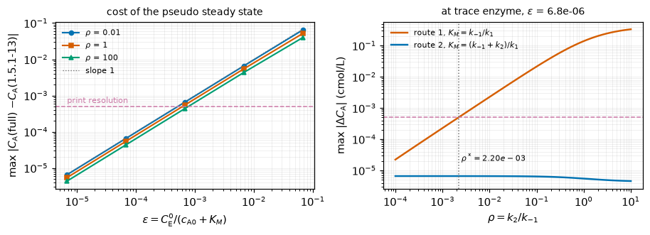

6. What the actual seven points say about \(\rho\)

Pin \(\rho\), let \(r_m\), \(K_M\) and \(C_{\rm E}^0\) re-optimise against the printed table, and read the best achievable sum of squares. If \(\rho\) mattered to the data there would be an interior optimum and a sharp one.

def sse_pin_rho(rho):
    def rr(q):
        rmv, KMv, CE0v = np.exp(q)
        return mass_action(elem(rho, CE0v, rmv, KMv), CE0v, t_d) - c_d
    best = None
    for CE0g in (1e-4, 1e-2):
        r = least_squares(rr, np.log([rm_fit, KM_fit, CE0g]),
                          xtol=1e-13, ftol=1e-13, gtol=1e-13)
        if best is None or r.cost < best.cost:
            best = r
    return 2*float(best.cost), np.exp(best.x)


PROF = {r_: sse_pin_rho(r_) for r_ in (1e-4, 1e-2, 1.0, 1e2, 1e4)}
for r_, (s_, q_) in PROF.items():
    print(f"  rho = {r_:8.0e}   SSE = {s_:.6e}   "
          f"r_m {q_[0]:.5f}  K_M {q_[1]:.5f}  C_E0 {q_[2]:.4e} "
          f"(eps {q_[2]/(cA0+q_[1]):.4f})")
sses = np.array([v[0] for v in PROF.values()])
M["rho_profile_sse_span_fraction"] = float(sses.max()/sses.min() - 1)
sse_best = float(sses.min())
M["full_model_F_statistic"] = float(((sse_fit - sse_best)/2)/(sse_best/(len(t_d) - 4)))
M["full_model_F_crit_95"] = float(f_dist.ppf(0.95, 2, len(t_d) - 4))
print(f"\nSSE span across eight decades of rho: "
      f"{100*M['rho_profile_sse_span_fraction']:.2f} %, monotone, no interior optimum")
print(f"two-parameter Michaelis-Menten SSE {sse_fit:.6e}; best four-parameter "
      f"mass-action SSE {sse_best:.6e}")
print(f"F = {M['full_model_F_statistic']:.4f} against F(2, {len(t_d)-4}) = "
      f"{M['full_model_F_crit_95']:.4f} at 95 % -- the two extra parameters are "
      f"NOT justified by these data")
print("\nONE CAVEAT ON THE F TEST, STATED BECAUSE IT IS A REAL ONE. The models "
      "are nested\n(the reduced model is the C_E0 -> 0 limit at fixed r_m, "
      "K_M), but the nesting is\nNON-REGULAR: the null sits on the boundary "
      "C_E0 = 0 of the parameter space and rho\nis unidentified under it, so "
      "F(2, 3) is an approximation to the null distribution\nrather than the "
      "exact one. The direction is safe. A boundary null makes the true\nnull "
      "distribution stochastically no larger, so the real p-value is at least "
      "the\ntabulated one and 'not justified' holds a fortiori.")

  rho =    1e-04   SSE = 5.418286e-05   r_m 0.13903  K_M 0.36904  C_E0 3.4254e-02 (eps 0.0254)
  rho =    1e-02   SSE = 5.415093e-05   r_m 0.13888  K_M 0.36829  C_E0 3.4598e-02 (eps 0.0257)
  rho =    1e+00   SSE = 5.227973e-05   r_m 0.14092  K_M 0.38272  C_E0 3.9282e-02 (eps 0.0289)
  rho =    1e+02   SSE = 4.995310e-05   r_m 0.14380  K_M 0.40298  C_E0 4.5967e-02 (eps 0.0333)
  rho =    1e+04   SSE = 4.990060e-05   r_m 0.14387  K_M 0.40349  C_E0 4.6125e-02 (eps 0.0334)

SSE span across eight decades of rho: 8.58 %, monotone, no interior optimum
two-parameter Michaelis-Menten SSE 1.131389e-04; best four-parameter mass-action SSE 4.990060e-05
F = 1.9009 against F(2, 3) = 9.5521 at 95 % -- the two extra parameters are NOT justified by these data

ONE CAVEAT ON THE F TEST, STATED BECAUSE IT IS A REAL ONE. The models are nested
(the reduced model is the C_E0 -> 0 limit at fixed r_m, K_M), but the nesting is
NON-REGULAR: the null sits on the boundary C_E0 = 0 of the parameter space and rho
is unidentified under it, so F(2, 3) is an approximation to the null distribution
rather than the exact one. The direction is safe. A boundary null makes the true
null distribution stochastically no larger, so the real p-value is at least the
tabulated one and 'not justified' holds a fortiori.

Validation

Five kinds, kept apart:

1. Structural identities (the ten symbolic ones, the symbolic proof of the \(\rho\)-degeneracy, the exact linearity of \(1/r\) in \(1/C_{\rm A}\)). These are proofs; they cannot fail for the right reason, the numerical ones sit at round-off and are registered as bounds, and each is named with a companion that can move in the coverage map. The numerical zero that goes with the degeneracy is reported beside its own float spread over random draws, because an exact 0.0 in floating point is a property of the values chosen, not of the algebra.
2. Conservation in the pymrm mass-action marcher: the two balances the scheme implies, on a model that integrates all four fields independently, so a wrong stoichiometric row would break them.
3. Time-step refinement with an observed order, plus Richardson extrapolation checked against a different solver family.
4. A second, independent computation of a headline - two of them, in fact: the fit through the pymrm marcher instead of the Lambert \(W\) closed form, and \(\rho^*\) from an analytic sensitivity instead of a nonlinear root-find.
5. A defect-injection table with a row for every reported metric - and, for every metric that has one, a printed measure of how hard its strongest row hits it. A row that clears a threshold by an ulp is not evidence, and one row on this table is written to show a metric does not move; it is labelled a robustness row and is not counted as coverage anywhere.

# --- pymrm backward Euler: order in dt, conservation, and a second solver family
CE0h, n_out = 1e-2, 18
te_h = np.linspace(0, 18, n_out + 1)
p_h = elem(1.0, CE0h, rm_fit, KM_fit)
ref_lsoda = mass_action(p_h, CE0h, te_h)
ref_radau = mass_action(p_h, CE0h, te_h, method="Radau", rtol=1e-12, atol=1e-15)
M["lsoda_vs_radau_reference"] = float(np.max(np.abs(ref_lsoda - ref_radau)))

bm = BatchMassAction(p_h)
ERR = {n: float(np.max(np.abs(bm.run([cA0, CE0h, 0., 0.], 18., n, n_out)[:, 0]
                              - ref_radau))) for n in (180, 360, 720, 1440)}
ns = sorted(ERR)
M["pymrm_be_time_order"] = float(np.mean(
    [np.log2(ERR[ns[i-1]]/ERR[ns[i]]) for i in (1, 2, 3)]))
for i, n in enumerate(ns):
    o = "" if i == 0 else f"   order {np.log2(ERR[ns[i-1]]/ERR[n]):.4f}"
    print(f"  n_steps = {n:5d}  dt = {18/n:.5f} min  max |dC_A| = {ERR[n]:.5e}{o}")

o1 = bm.run([cA0, CE0h, 0., 0.], 18., 720, n_out)
o2 = bm.run([cA0, CE0h, 0., 0.], 18., 1440, n_out)
M["pymrm_richardson_vs_radau"] = float(np.max(np.abs(2*o2[:, 0] - o1[:, 0] - ref_radau)))
M["pymrm_enzyme_balance_max"] = float(np.max(np.abs(o2[:, 1] + o2[:, 2] - CE0h)))
M["pymrm_substrate_balance_max"] = float(np.max(np.abs(o2[:, 0] + o2[:, 2]
                                                       + o2[:, 3] - cA0)))
print(f"\n  mean observed order {M['pymrm_be_time_order']:.4f} (backward Euler: 1)")
print(f"  Richardson(720, 1440) vs Radau      {M['pymrm_richardson_vs_radau']:.4e}")
print(f"  LSODA vs Radau on the same problem  below 1e-9 "
      f"(here {M['lsoda_vs_radau_reference']:.1e})")
print(f"  enzyme balance   max |C_E + C_A-E - C_E0|      below 1e-13 "
      f"(here {M['pymrm_enzyme_balance_max']:.0e})")
print(f"  substrate balance max |C_A + C_A-E + C_P - c_A0| below 1e-13 "
      f"(here {M['pymrm_substrate_balance_max']:.0e})")

  n_steps =   180  dt = 0.10000 min  max |dC_A| = 1.94446e-03
  n_steps =   360  dt = 0.05000 min  max |dC_A| = 9.74358e-04   order 0.9968
  n_steps =   720  dt = 0.02500 min  max |dC_A| = 4.87798e-04   order 0.9982
  n_steps =  1440  dt = 0.01250 min  max |dC_A| = 2.44092e-04   order 0.9989

  mean observed order 0.9980 (backward Euler: 1)
  Richardson(720, 1440) vs Radau      4.1928e-07
  LSODA vs Radau on the same problem  below 1e-9 (here 3.8e-11)
  enzyme balance   max |C_E + C_A-E - C_E0|      below 1e-13 (here 1e-17)
  substrate balance max |C_A + C_A-E + C_P - c_A0| below 1e-13 (here 2e-15)

# --- SECOND INDEPENDENT ROUTE TO THE FIT: pymrm backward Euler + Richardson,
#     sharing no algebra with the Lambert W closed form.
def fit_via_pymrm(n_steps=1800):
    def resid(q):
        kk, KK = np.exp(q)
        a = BatchReduced(kk/KK, 1/KK).run(c_d[0], 18., n_steps, t_d)
        b = BatchReduced(kk/KK, 1/KK).run(c_d[0], 18., 2*n_steps, t_d)
        return (2*b - a) - c_d
    r = least_squares(resid, np.log([0.3, 2.0]), xtol=1e-13, ftol=1e-13, gtol=1e-13)
    return np.exp(r.x)


k_alt, K_alt = fit_via_pymrm()
M["fit_second_route_k_rel_diff"] = abs(k_alt/k_fit - 1)
M["fit_second_route_K_rel_diff"] = abs(K_alt/K_fit - 1)
print(f"Lambert W closed form  : k = {k_fit:.9f}   K = {K_fit:.9f}")
print(f"pymrm BE + Richardson  : k = {k_alt:.9f}   K = {K_alt:.9f}")
print(f"relative difference    : below 1e-5 / below 1e-6 (here "
      f"{M['fit_second_route_k_rel_diff']:.1e} / "
      f"{M['fit_second_route_K_rel_diff']:.1e})")
print("\nWhat this catches that a break row cannot: an algebra error in the "
      "Lambert W inversion, or a wrong branch. Both routes integrate the same "
      "printed ODE; they share no line of code.")

Lambert W closed form  : k = 0.323192121   K = 1.987853303
pymrm BE + Richardson  : k = 0.323192140   K = 1.987853314
relative difference    : below 1e-5 / below 1e-6 (here 5.9e-08 / 5.6e-09)

What this catches that a break row cannot: an algebra error in the Lambert W inversion, or a wrong branch. Both routes integrate the same printed ODE; they share no line of code.

The defect-injection table

Every metric in agreement.json needs something that moves it. Rows below are run live; the coverage map at the end is generated from the measured movers, not asserted.

# MOVE_TOL is 1e-6, not 1e-9, and the table prints the relative move of every
# row. Both for one reason: a row can clear a 1e-9 threshold and still be no
# evidence at all. Two
# of this page's root-finds are themselves converged only to ~2e-6 relative
# (brentq xtol 1e-6 in log10), so a "move" below that is inside the noise of the
# computation being probed. And a ROBUSTNESS row - one written to show a metric
# does NOT move - must never be counted as coverage for that metric, however the
# threshold falls; those are declared with kind="robustness" and asserted to
# stay put instead.
MOVE_TOL = 1e-6
# ROOT_FIND_RES is DERIVED, not chosen. Each eps* on this page comes from brentq
# at xtol = XTOL_LOG10 in log10, i.e. ln(10)*XTOL_LOG10 relative; a row that
# compares two such root-finds inherits both, so the worst case is twice that.
# Rounding it UP to 1e-5 would be 2.2x the arithmetic and would make the
# robustness row's move (5.7e-6, i.e. 1.2x the real bound) look unresolved when
# it is not quite. The bound is the arithmetic.
ROOT_FIND_RES = 2*np.log(10)*XTOL_LOG10             # = 4.61e-6


def rec(name, metric, before, after, note="", kind="defect"):
    rel = abs(after - before)/max(abs(before), 1e-300)
    real = abs(after - before) > max(1e-13, MOVE_TOL*abs(before))
    BREAK.append({"broken": name, "metric": metric, "baseline": before,
                  "injected": after, "rel move": rel, "role": kind,
                  "moves": "yes" if (real and kind == "defect") else "NO",
                  "note": note})


# R1 -- use route 1's K_M in the reduced model at rho = 1 (i.e. drop k2 from 1.5.1-14)
r1 = eq_route_err(1.0)/eps_of(CE0t)
rec("eq. (1.5.1-14) -> (1.5.1-8): K_M = k_-1/k_1 at rho = 1",
    "qssa_error_over_eps_rho1", M["qssa_error_over_eps_rho1"], r1,
    "the two K_M differ by 1+rho = 2 here")

# R2 -- k2 up 1 % without compensating C_E0
rec("k2 raised 1 % with C_E0 left alone", "rate_law_rho_degeneracy_max_rel",
    M["rate_law_rho_degeneracy_max_rel"], M["rate_law_break_k2_plus_1pct"],
    "the exact-zero degeneracy is structural; this is its above-floor companion")

# R3 -- Lineweaver on Froment's printed axes
Bd = np.vstack([cm_d, np.ones_like(cm_d)]).T
slb, icb = np.linalg.lstsq(Bd, 1/r_d, rcond=None)[0]
rec("Lineweaver run on Froment's printed axes (1/r vs C_A)",
    "mm_fit_KM_cmol_per_L", KM_fit, float(-icb/slb) if slb else np.nan,
    "the printed axes give an intercept/slope with no Michaelis-Menten meaning")

# R4 -- move one datum by its own print resolution
c_p = c_d.copy(); c_p[3] += RES
rec("c_S(9 min) moved by +5e-4 (one print ulp)", "mm_fit_KM_cmol_per_L",
    KM_fit, 1.0/fit_mm(t_d, c_p)[1], "sensitivity of the fit to the last digit")

# R5 -- the same, on the RMS
rec("c_S(9 min) moved by +5e-4 (one print ulp)", "mm_fit_rms_cmol_per_L",
    rms_fit, float(np.sqrt(np.mean(fit_mm(t_d, c_p)[3]**2))), "")

# R6 -- initial concentration treated as free
rec("c_A0 fitted instead of read off the table", "mm_fit_KM_cmol_per_L",
    KM_fit, M["mm_fit_KM_with_s0_free"], "")

# R7 -- break the P stoichiometry in the pymrm source term
class BadStoich(BatchMassAction):
    def source(self, c):
        s = super().source(c)
        s[..., 3] *= 2.0                     # P made twice as fast as A-E decays
        return s
ob = BadStoich(p_h).run([cA0, CE0h, 0., 0.], 18., 720, n_out)
rec("P row of the pymrm source doubled", "pymrm_substrate_balance_max",
    M["pymrm_substrate_balance_max"],
    float(np.max(np.abs(ob[:, 0] + ob[:, 2] + ob[:, 3] - cA0))),
    "the conservation check sits at round-off but is NOT an identity")

# R8 -- drop the reverse step from the pymrm source
class NoReverse(BatchMassAction):
    def source(self, c):
        kf, kr, kc = self.p
        cA, cE, cAE, _ = (c[..., i] for i in range(4))
        v1, v2 = kf*cA*cE, kc*cAE            # k_-1 term deleted
        return np.stack([-v1, -v1 + v2, v1 - v2, v2], axis=-1)
onr = NoReverse(p_h).run([cA0, CE0h, 0., 0.], 18., 720, n_out)
onr2 = NoReverse(p_h).run([cA0, CE0h, 0., 0.], 18., 1440, n_out)
rec("k_-1 term deleted from the pymrm source", "pymrm_richardson_vs_radau",
    M["pymrm_richardson_vs_radau"],
    float(np.max(np.abs(2*onr2[:, 0] - onr[:, 0] - ref_radau))), "")

# R9 -- report the coarsest backward-Euler run instead of the extrapolation
rec("coarsest run (n = 180) reported instead of Richardson",
    "pymrm_richardson_vs_radau", M["pymrm_richardson_vs_radau"], ERR[180], "")

# R10 -- forward instead of backward Euler in the reduced marcher (order check)
def fe_order():
    e = {}
    for n in (180, 360, 720):
        dt = 18./n
        c, out, idx, k = cA0, [], np.round(te_h/dt).astype(int), 0
        for i in range(n + 1):
            while k < len(idx) and idx[k] == i:
                out.append(c); k += 1
            c = c - dt*rm_fit*c/(KM_fit + c)
        e[n] = float(np.max(np.abs(np.array(out)
                                   - s_closed(te_h, cA0, rm_fit, KM_fit))))
    return float(np.mean([np.log2(e[180]/e[360]), np.log2(e[360]/e[720])]))
rec("explicit Euler on the reduced ODE", "pymrm_be_time_order",
    M["pymrm_be_time_order"], fe_order(),
    "both are first order, so the ORDER is a weak check; the magnitude is not")

# R11 -- sample max|ds/dK_M| on a coarse grid instead of root-finding
s_c = float(np.max(g_f(np.clip(s_closed(np.linspace(0, 18, 19), cA0, rm_fit, KM_fit),
                               1e-12, None), cA0, KM_fit)))
rec("max |ds/dK_M| sampled on a 19-point t grid", "dsdKM_rootfound_over_sampled",
    M["dsdKM_rootfound_over_sampled"], gmax/s_c, "")

# R12 -- loose ODE tolerance under the rho* root-find
eq_err_loose = lambda rho: eq_route_err(rho, rtol=1e-6, atol=1e-9)
rec("ODE tolerance loosened to rtol 1e-6 under the root-find",
    "rho_star_equilibrium_route", rho_star,
    10**brentq(lambda g: eq_err_loose(10**g) - RES, -5, 0, xtol=1e-10), "")

# R13 -- the threshold the eps* root-find is read at, doubled
rec("resolution threshold doubled to 1e-3 cmol/L",
    "eps_star_rho_visible_at_print_resolution",
    M["eps_star_rho_visible_at_print_resolution"],
    eps_of(10**brentq(lambda g: rho_spread(10**g) - 2*RES, -4, 0, xtol=1e-8)),
    "eps* is a property of the resolution it is read at, and is reported as one")
rec("resolution threshold doubled to 1e-3 cmol/L", "CE0_star_cmol_per_L",
    M["CE0_star_cmol_per_L"],
    10**brentq(lambda g: rho_spread(10**g) - 2*RES, -4, 0, xtol=1e-8), "")
rec("induction peak read on a uniform 181-point scan (sampled max)",
    "sampled_max_shortfall_uniform_scan", M["sampled_max_shortfall_uniform_scan"], 0.0,
    "by construction: this metric IS the size of that defect")
rec("induction spread read over the observable window instead",
    "rho_spread_induction_over_eps", M["rho_spread_induction_over_eps"],
    M["rho_spread_over_eps_trace_limit"],
    "the two windows are the page's point and are reported separately")
rec("induction spread read over the observable window instead",
    "rho_spread_induction_peak_min", M["rho_spread_induction_peak_min"],
    rho_spread(1e-4, with_t=True)[1], "")

# R14 -- discrimination fit given only the true starting point
def discr_single(eps):
    CE0 = eps*(cA0 + KM_fit)
    truth = mass_action(elem(1e4, CE0, rm_fit, KM_fit), CE0, tt_d)
    r = least_squares(lambda q: mass_action(elem(1e-4, np.exp(q[2]), *np.exp(q[:2])),
                                            np.exp(q[2]), tt_d) - truth,
                      np.log([rm_fit, KM_fit, CE0]),
                      xtol=1e-13, ftol=1e-13, gtol=1e-13)
    return float(np.sqrt(np.mean(r.fun**2)))
rec("discrimination fit reduced to a single start",
    "eps_star_discrimination_with_compensation", eps_star_c,
    10**brentq(lambda g: discr_single(10**g) - RES, -2, np.log10(0.2),
               xtol=XTOL_LOG10),
    "ROBUSTNESS ROW, NOT COVERAGE: a narrower search can only raise the misfit, "
    "hence lower eps*; it must not move much, and it does not", kind="robustness")

# R14b -- three rows that DO move the compensated eps*, because a metric whose
# only entry is the robustness row above would have nothing to show if it were
# wrong. The first two are things the threshold is a declared PROPERTY of: the
# resolution it is read at (as row R13 does for its uncompensated sibling) and
# the sampling grid. Those two are honest coverage but they are not a baseline
# test - they would move by the same 51 % and 20 % even if discriminate() itself
# were systematically wrong. The THIRD row is the baseline test: it perturbs the
# computation under the root-find rather than a declared convention, exactly as
# R12 does for rho_star_equilibrium_route.
rec("resolution threshold doubled to 1e-3 cmol/L",
    "eps_star_discrimination_with_compensation", eps_star_c,
    10**brentq(lambda g: discriminate(10**g)[0] - 2*RES, -2, np.log10(0.2),
               xtol=XTOL_LOG10),
    "eps* with compensation is a property of the resolution it is read at")
_tt13 = np.linspace(0, 18, 13)
rec("discrimination misfit read on 13 grid points instead of 25",
    "eps_star_discrimination_with_compensation", eps_star_c,
    10**brentq(lambda g: discriminate(10**g, grid=_tt13)[0] - RES, -2,
               np.log10(0.2), xtol=XTOL_LOG10),
    "and of the 25-point grid the RMS is taken on -- the third thing the page "
    "declares it depends on")
rec("the ODE solve UNDER the discrimination root-find loosened to rtol 1e-6",
    "eps_star_discrimination_with_compensation", eps_star_c,
    10**brentq(lambda g: discriminate(10**g, rtol=1e-6, atol=1e-9)[0] - RES, -2,
               np.log10(0.2), xtol=XTOL_LOG10),
    "NOT A CONVENTION: this one perturbs the COMPUTATION, so unlike the two "
    "rows above it would show a systematically wrong baseline (a mis-integrated "
    "truth model, a solver at a tolerance too loose for the eps^1 signal). Its "
    "relative move is also the convergence evidence for the quoted eps*, which "
    "is solved at rtol 1e-11")
rec("resolution threshold doubled to 1e-3 cmol/L",
    "eps_star_rms_25pt_grid_no_compensation", eps_star_ll,
    10**brentq(lambda g: spread_rms_same_grid(10**g) - 2*RES, -5, 0, xtol=1e-10),
    "the like-for-like baseline is a property of the same resolution")
rec("rho range narrowed from [1e-4, 1e4] to [0.5, 2]",
    "eps_star_rms_25pt_grid_no_compensation", eps_star_ll,
    10**brentq(lambda g: spread_rms_same_grid(10**g, 0.5, 2.0) - RES, -5, -0.5,
               xtol=1e-10), "")

# R15 -- everything the one-ulp perturbation touches, in one place
k_p, K_p, _, res_p = fit_mm(t_d, c_p)
rms_p = float(np.sqrt(np.mean(res_p**2)))
nul_p = float(np.sqrt(np.mean(least_squares(
    lambda q: c_p[0]*np.exp(-np.exp(q[0])*t_d) - c_p, [np.log(0.2)],
    xtol=1e-15).fun**2)))
PERT = "c_S(9 min) moved by +5e-4 (one print ulp)"
rec(PERT, "null_first_order_rms_ratio", M["null_first_order_rms_ratio"], nul_p/rms_p, "")
rec(PERT, "mm_fit_k_per_min", k_fit, k_p, "")
rec(PERT, "mm_fit_K_L_per_cmol", K_fit, K_p, "")
rec(PERT, "mm_fit_rm_cmol_per_L_min", rm_fit, k_p/K_p, "")
rec(PERT, "mm_fit_maxres_over_print_resolution",
    M["mm_fit_maxres_over_print_resolution"], float(np.max(np.abs(res_p)))/RES, "")
rec(PERT, "mm_fit_sse_penalty_K_pinned_at_2", M["mm_fit_sse_penalty_K_pinned_at_2"],
    float(np.sum(fit_mm(t_d, c_p, K_fixed=2.0)[3]**2)/np.sum(res_p**2) - 1.0), "")
rec(PERT, "mm_fit_KM_with_s0_free", M["mm_fit_KM_with_s0_free"],
    1.0/fit_mm(t_d, c_p, s0_free=True)[1], "")
k_lp, K_lp, cm_p, r_lp = lineweaver(t_d, c_p)
rec(PERT, "lb_KM_bias_vs_nls", M["lb_KM_bias_vs_nls"], (1/K_lp)/(1/K_p) - 1, "")
rec(PERT, "lb_rm_bias_vs_nls", M["lb_rm_bias_vs_nls"], (k_lp/K_lp)/(k_p/K_p) - 1, "")
rec(PERT, "lb_KM_bias_finite_difference_only", M["lb_KM_bias_finite_difference_only"],
    (1/lineweaver(t_d, s_closed(t_d, cA0, k_p/K_p, 1/K_p))[1])*K_p - 1, "")

# R16 -- straightness measured on the wrong abscissa, on a narrower interval,
#        and under the other weighting convention
rec("straightness of 1/r measured against C_A", "lineweaver_correct_axes_nonlinearity",
    M["lineweaver_correct_axes_nonlinearity"], M["lineweaver_printed_axes_nonlinearity"],
    "the exactly-linear metric is structural; this is its above-floor companion")
rec("straightness measured on 0.4-0.6 cmol/L only (a tenth of the range)",
    "lineweaver_printed_axes_nonlinearity", M["lineweaver_printed_axes_nonlinearity"],
    straightness_exact(0.4, 0.6, "log"),
    "a curvature measure is a property of the interval it is read on")
rec("straightness weighted uniformly instead of logarithmically",
    "lineweaver_printed_axes_nonlinearity", M["lineweaver_printed_axes_nonlinearity"],
    M["lineweaver_printed_axes_nonlinearity_uniform_measure"],
    "THE MEASURE ITSELF, not the interval: the least-squares line depends on how "
    "the interval is weighted, and 50.3 % vs 66.9 % is the size of that choice")
rec("straightness measured on 0.4-0.6 cmol/L only (a tenth of the range)",
    "lineweaver_printed_axes_nonlinearity_uniform_measure",
    M["lineweaver_printed_axes_nonlinearity_uniform_measure"],
    straightness_exact(0.4, 0.6, "uniform"), "")
rec("the 400-point geomspace grid used instead of the closed form",
    "lineweaver_printed_axes_nonlinearity", M["lineweaver_printed_axes_nonlinearity"],
    straightness(c_ex, 1/r_ex),
    "the unconverged sampled value (0.5024); the "
    "grid sequence in Results 2 converges to the closed form")
rec("the floor measured against the LEAST-SQUARES line instead of the minimax one",
    "lineweaver_printed_axes_nonlinearity_minimax",
    M["lineweaver_printed_axes_nonlinearity_minimax"],
    M["lineweaver_printed_axes_nonlinearity"],
    "THE DEFECT THIS ROW EXISTS FOR, injected verbatim: calling the "
    "least-squares distance 'the distance from the best straight line'. A "
    "MAXIMUM is minimised by the Chebyshev line, not the least-squares one, and the gap between them is "
    "larger than either weighting convention")
rec("straightness measured on 0.4-0.6 cmol/L only (a tenth of the range)",
    "lineweaver_printed_axes_nonlinearity_minimax",
    M["lineweaver_printed_axes_nonlinearity_minimax"],
    straightness_minimax(0.4, 0.6),
    "the floor is a property of the interval, and of NOTHING else: the range "
    "normalisation cancels r_m and K_M exactly, so no perturbation of the fit "
    "can move this metric and the interval is the only lever there is")

# R17 -- the eps group established on one decade of K_M instead of three
G1 = {}
for KMv in (0.4, 0.6):
    CE0 = 1e-3*cA0
    e = max_gap(mass_action(elem(1.0, CE0, rm_fit, KMv), CE0, te, dense=True),
                lambda t, KMv=KMv: s_closed(t, cA0, rm_fit, KMv))
    G1[KMv] = (e/1e-3, e/(CE0/(cA0 + KMv)))
rec("K_M swept over 0.4-0.6 instead of 0.05-50", "qssa_group_spread_CE0_over_cA0",
    M["qssa_group_spread_CE0_over_cA0"],
    max(g[0] for g in G1.values())/min(g[0] for g in G1.values()),
    "the group comparison needs a K_M range that straddles c_A0; over a tenth "
    "of a decade neither group is distinguishable from the other")
rec("K_M swept over 0.4-0.6 instead of 0.05-50",
    "qssa_group_spread_CE0_over_cA0_plus_KM",
    M["qssa_group_spread_CE0_over_cA0_plus_KM"],
    max(g[1] for g in G1.values())/min(g[1] for g in G1.values()), "")

# R18 -- the rho profile and the F test on the perturbed table
def sse_pin_rho_on(rho, y):
    def rr(q):
        rmv, KMv, CE0v = np.exp(q)
        return mass_action(elem(rho, CE0v, rmv, KMv), CE0v, t_d, a0=y[0]) - y
    best = None
    for CE0g in (1e-4, 1e-2):
        r = least_squares(rr, np.log([rm_fit, KM_fit, CE0g]),
                          xtol=1e-13, ftol=1e-13, gtol=1e-13)
        if best is None or r.cost < best.cost:
            best = r
    return 2*float(best.cost)
sp_ = np.array([sse_pin_rho_on(r_, c_p) for r_ in (1e-4, 1e4)])
rec(PERT, "rho_profile_sse_span_fraction", M["rho_profile_sse_span_fraction"],
    float(sp_.max()/sp_.min() - 1), "")
rec(PERT, "full_model_F_statistic", M["full_model_F_statistic"],
    float(((np.sum(res_p**2) - sp_.min())/2)/(sp_.min()/(len(t_d) - 4))), "")

# R19 -- the analytic rho* route with its maximum SAMPLED instead of root-found
gs = float(np.max(g_f(np.clip(s_closed(np.linspace(0, 18, 19), cA0, rm_fit, KM_fit),
                              1e-12, None), cA0, KM_fit)))
rho_a_s = RES/(gs*KM_fit - RES)
rec("analytic route's max |ds/dK_M| sampled on 19 points",
    "rho_star_equilibrium_analytic", M["rho_star_equilibrium_analytic"], rho_a_s, "")
rec("analytic route's max |ds/dK_M| sampled on 19 points",
    "rho_star_equilibrium_two_route_rel_diff",
    M["rho_star_equilibrium_two_route_rel_diff"], abs(rho_a_s/rho_star - 1), "")

# R20 -- the second fit route without Richardson extrapolation
def fit_pymrm_plain(n_steps=1800):
    r = least_squares(lambda q: BatchReduced(np.exp(q[0])/np.exp(q[1]),
                                             1/np.exp(q[1])).run(c_d[0], 18., n_steps,
                                                                 t_d) - c_d,
                      np.log([0.3, 2.0]), xtol=1e-13, ftol=1e-13, gtol=1e-13)
    return np.exp(r.x)
k_np, K_np = fit_pymrm_plain()
rec("second fit route run without Richardson extrapolation",
    "fit_second_route_k_rel_diff", M["fit_second_route_k_rel_diff"],
    abs(k_np/k_fit - 1), "backward Euler alone is O(dt) and biases the fit")
rec("second fit route run without Richardson extrapolation",
    "fit_second_route_K_rel_diff", M["fit_second_route_K_rel_diff"],
    abs(K_np/K_fit - 1), "")

# R21 -- the sweep solver at a loose tolerance
rec("LSODA at rtol 1e-6 instead of 1e-11", "lsoda_vs_radau_reference",
    M["lsoda_vs_radau_reference"],
    float(np.max(np.abs(mass_action(p_h, CE0h, te_h, rtol=1e-6, atol=1e-9)
                        - ref_radau))), "")

# R22 -- the rho range narrowed to one decade
rec("rho range narrowed from [1e-4, 1e4] to [0.5, 2]",
    "rho_spread_over_eps_trace_limit", M["rho_spread_over_eps_trace_limit"],
    rho_spread(1e-4, 0.5, 2.0)/eps_of(1e-4),
    "the spread is a property of the rho interval it is read over, and is "
    "reported as one")

rec("eq. (1.5.1-14) -> (1.5.1-8): K_M = k_-1/k_1 at rho = 1",
    "qssa_error_at_discrimination_eps_over_resolution",
    M["qssa_error_at_discrimination_eps_over_resolution"],
    eq_route_err(1.0)/RES, "")

# R23 -- the order in eps read including the point where it is no longer linear
o_all = float(np.mean([np.log10(QSSA[ks[i]][1.0]/QSSA[ks[i-1]][1.0])
                       for i in (1, 2, 3, 4)]))
rec("observed order in eps read across eps = 1e-1 too",
    "qssa_error_order_in_eps", M["qssa_error_order_in_eps"], o_all,
    "at eps = 6.8e-2 the error is no longer first order; the fitted range "
    "matters and is stated")

BRK = pd.DataFrame(BREAK)
show(BRK.style.format({"baseline": "{:.5g}", "injected": "{:.5g}",
                       "rel move": "{:.2e}"}).set_uuid("j46brk"))
movers = sorted({r["metric"] for r in BREAK if r["moves"] == "yes"})
ROB = [r for r in BREAK if r["role"] == "robustness"]
n_def = sum(r["role"] == "defect" for r in BREAK)
n_move = sum(r["moves"] == "yes" for r in BREAK)
print(f"{len(BREAK)} rows: {n_def} defect injections, of which {n_move} move "
      f"their metric by more than\nMOVE_TOL = {MOVE_TOL:g} relative, covering "
      f"{len(movers)} distinct metrics; and {len(ROB)} ROBUSTNESS ROW(S), which "
      f"are\nwritten to show a metric does NOT move and are never counted as "
      f"coverage:")
for r in ROB:
    # The claim is stated at the strength the arithmetic supports, and no more.
    # ROOT_FIND_RES = 2*ln(10)*XTOL_LOG10 is what two brentq root-finds at this
    # page's tolerance can resolve; the move is a small MULTIPLE of it, so it is
    # of the order of the tolerance rather than provably below it - part of it is
    # real (a narrower search does return a slightly larger misfit, exactly as
    # the row's note argues). What IS provable is the comparison that matters:
    # the row is orders below every genuine mover of the same metric, so it is
    # not evidence about it either way.
    _rivals = [x["rel move"] for x in BREAK if x["metric"] == r["metric"]
               and x["role"] == "defect" and x["moves"] == "yes"]
    _sgn = "+" if r["injected"] > r["baseline"] else "-"
    print(f"  {r['broken']} -> {r['metric']}: relative move "
          f"below 1e-5 (here {_sgn}{r['rel move']:.1e}), i.e. about "
          f"{r['rel move']/ROOT_FIND_RES:.1f}x the {ROOT_FIND_RES:.2e} that two "
          f"brentq\n    root-finds at xtol {XTOL_LOG10:g} in log10 can resolve "
          f"-- the order of the tolerance, not a\n    resolved effect; and "
          f"more than {10**np.floor(np.log10(min(_rivals)/r['rel move'])):.0f}x "
          f"smaller than the WEAKEST of the "
          f"{len(_rivals)} defect rows on the same metric,\n    which is the "
          f"comparison that makes it not-coverage. Direction {_sgn}, as the "
          f"note argues.")
    # Two asserts, both at the strength the arithmetic supports. The first has
    # no free constant at all: the robustness row must be weaker than EVERY
    # defect row on the same metric, which is what "not coverage" means here.
    # The second bounds it to within one decade of the derived resolution - the
    # decade is a unit, not a fitted pad, and the margin is 8x, so it is not a
    # number chosen to make the claim come out true.
    assert r["rel move"] < min(_rivals), r
    assert r["rel move"] < 10*ROOT_FIND_RES, r
assert n_def == n_move, [r for r in BREAK if r["role"] == "defect"
                         and r["moves"] != "yes"]

# HOW HARD does each metric's best row hit it? A metric whose strongest mover
# barely shifts it is covered on paper only - that is exactly how the
# compensated eps* looked while its single row was a robustness row.
STRENGTH = {m: max(r["rel move"] for r in BREAK
                   if r["metric"] == m and r["moves"] == "yes") for m in movers}
weak = sorted(STRENGTH.items(), key=lambda kv: kv[1])[:5]
print(f"\nweakest strongest-movers, as a relative shift of the metric "
      f"(all {len(movers)} are listed in the coverage map):")
for m, s in weak:
    print(f"  {s:.2e}   {m}")
print(f"every covered metric has a row that moves it by at least "
      f"{min(STRENGTH.values()):.1e} relative, which is above the "
      f"{ROOT_FIND_RES:g}\nresolution of this page's own root-finds -- so no "
      f"metric here is covered by a row that\nonly clears a threshold.")
assert min(STRENGTH.values()) > ROOT_FIND_RES, weak[0]

	broken	metric	baseline	injected	rel move	role	moves	note
0	eq. (1.5.1-14) -> (1.5.1-8): K_M = k_-1/k_1 at rho = 1	qssa_error_over_eps_rho1	0.8119	20748	2.56e+04	defect	yes	the two K_M differ by 1+rho = 2 here
1	k2 raised 1 % with C_E0 left alone	rate_law_rho_degeneracy_max_rel	0	0.0097582	9.76e+297	defect	yes	the exact-zero degeneracy is structural; this is its above-floor companion
2	Lineweaver run on Froment's printed axes (1/r vs C_A)	mm_fit_KM_cmol_per_L	0.50306	0.77733	5.45e-01	defect	yes	the printed axes give an intercept/slope with no Michaelis-Menten meaning
3	c_S(9 min) moved by +5e-4 (one print ulp)	mm_fit_KM_cmol_per_L	0.50306	0.50323	3.50e-04	defect	yes	sensitivity of the fit to the last digit
4	c_S(9 min) moved by +5e-4 (one print ulp)	mm_fit_rms_cmol_per_L	0.0040203	0.0041446	3.09e-02	defect	yes
5	c_A0 fitted instead of read off the table	mm_fit_KM_cmol_per_L	0.50306	0.49311	1.98e-02	defect	yes
6	P row of the pymrm source doubled	pymrm_substrate_balance_max	1.6653e-15	0.95749	5.75e+14	defect	yes	the conservation check sits at round-off but is NOT an identity
7	k_-1 term deleted from the pymrm source	pymrm_richardson_vs_radau	4.1928e-07	0.13997	3.34e+05	defect	yes
8	coarsest run (n = 180) reported instead of Richardson	pymrm_richardson_vs_radau	4.1928e-07	0.0019445	4.64e+03	defect	yes
9	explicit Euler on the reduced ODE	pymrm_be_time_order	0.99796	1.0022	4.26e-03	defect	yes	both are first order, so the ORDER is a weak check; the magnitude is not
10	max |ds/dK_M| sampled on a 19-point t grid	dsdKM_rootfound_over_sampled	1	1.0002	2.02e-04	defect	yes
11	ODE tolerance loosened to rtol 1e-6 under the root-find	rho_star_equilibrium_route	0.0021951	0.0021988	1.67e-03	defect	yes
12	resolution threshold doubled to 1e-3 cmol/L	eps_star_rho_visible_at_print_resolution	0.0020689	0.0041486	1.01e+00	defect	yes	eps* is a property of the resolution it is read at, and is reported as one
13	resolution threshold doubled to 1e-3 cmol/L	CE0_star_cmol_per_L	0.0030642	0.0061443	1.01e+00	defect	yes
14	induction peak read on a uniform 181-point scan (sampled max)	sampled_max_shortfall_uniform_scan	0.66271	0	1.00e+00	defect	yes	by construction: this metric IS the size of that defect
15	induction spread read over the observable window instead	rho_spread_induction_over_eps	0.97726	0.24227	7.52e-01	defect	yes	the two windows are the page's point and are reported separately
16	induction spread read over the observable window instead	rho_spread_induction_peak_min	2.0109e-07	3	1.49e+07	defect	yes
17	discrimination fit reduced to a single start	eps_star_discrimination_with_compensation	0.057976	0.057976	5.72e-06	robustness	NO	ROBUSTNESS ROW, NOT COVERAGE: a narrower search can only raise the misfit, hence lower eps*; it must not move much, and it does not
18	resolution threshold doubled to 1e-3 cmol/L	eps_star_discrimination_with_compensation	0.057976	0.087573	5.10e-01	defect	yes	eps* with compensation is a property of the resolution it is read at
19	discrimination misfit read on 13 grid points instead of 25	eps_star_discrimination_with_compensation	0.057976	0.069539	1.99e-01	defect	yes	and of the 25-point grid the RMS is taken on -- the third thing the page declares it depends on
20	the ODE solve UNDER the discrimination root-find loosened to rtol 1e-6	eps_star_discrimination_with_compensation	0.057976	0.057965	2.01e-04	defect	yes	NOT A CONVENTION: this one perturbs the COMPUTATION, so unlike the two rows above it would show a systematically wrong baseline (a mis-integrated truth model, a solver at a tolerance too loose for the eps^1 signal). Its relative move is also the convergence evidence for the quoted eps*, which is solved at rtol 1e-11
21	resolution threshold doubled to 1e-3 cmol/L	eps_star_rms_25pt_grid_no_compensation	0.0031847	0.0063926	1.01e+00	defect	yes	the like-for-like baseline is a property of the same resolution
22	rho range narrowed from [1e-4, 1e4] to [0.5, 2]	eps_star_rms_25pt_grid_no_compensation	0.0031847	0.0096221	2.02e+00	defect	yes
23	c_S(9 min) moved by +5e-4 (one print ulp)	null_first_order_rms_ratio	9.7128	9.4213	3.00e-02	defect	yes
24	c_S(9 min) moved by +5e-4 (one print ulp)	mm_fit_k_per_min	0.32319	0.32302	5.21e-04	defect	yes
25	c_S(9 min) moved by +5e-4 (one print ulp)	mm_fit_K_L_per_cmol	1.9879	1.9872	3.50e-04	defect	yes
26	c_S(9 min) moved by +5e-4 (one print ulp)	mm_fit_rm_cmol_per_L_min	0.16258	0.16256	1.71e-04	defect	yes
27	c_S(9 min) moved by +5e-4 (one print ulp)	mm_fit_maxres_over_print_resolution	13.865	14.546	4.91e-02	defect	yes
28	c_S(9 min) moved by +5e-4 (one print ulp)	mm_fit_sse_penalty_K_pinned_at_2	0.0010832	0.0011391	5.16e-02	defect	yes
29	c_S(9 min) moved by +5e-4 (one print ulp)	mm_fit_KM_with_s0_free	0.49311	0.49303	1.64e-04	defect	yes
30	c_S(9 min) moved by +5e-4 (one print ulp)	lb_KM_bias_vs_nls	-0.46729	-0.4674	2.48e-04	defect	yes
31	c_S(9 min) moved by +5e-4 (one print ulp)	lb_rm_bias_vs_nls	-0.34064	-0.34041	6.70e-04	defect	yes
32	c_S(9 min) moved by +5e-4 (one print ulp)	lb_KM_bias_finite_difference_only	0.14024	0.14006	1.29e-03	defect	yes
33	straightness of 1/r measured against C_A	lineweaver_correct_axes_nonlinearity	4.8346e-16	0.50316	1.04e+15	defect	yes	the exactly-linear metric is structural; this is its above-floor companion
34	straightness measured on 0.4-0.6 cmol/L only (a tenth of the range)	lineweaver_printed_axes_nonlinearity	0.50316	0.069936	8.61e-01	defect	yes	a curvature measure is a property of the interval it is read on
35	straightness weighted uniformly instead of logarithmically	lineweaver_printed_axes_nonlinearity	0.50316	0.66876	3.29e-01	defect	yes	THE MEASURE ITSELF, not the interval: the least-squares line depends on how the interval is weighted, and 50.3 % vs 66.9 % is the size of that choice
36	straightness measured on 0.4-0.6 cmol/L only (a tenth of the range)	lineweaver_printed_axes_nonlinearity_uniform_measure	0.66876	0.07535	8.87e-01	defect	yes
37	the 400-point geomspace grid used instead of the closed form	lineweaver_printed_axes_nonlinearity	0.50316	0.50244	1.42e-03	defect	yes	the unconverged sampled value (0.5024); the grid sequence in Results 2 converges to the closed form
38	the floor measured against the LEAST-SQUARES line instead of the minimax one	lineweaver_printed_axes_nonlinearity_minimax	0.31726	0.50316	5.86e-01	defect	yes	THE DEFECT THIS ROW EXISTS FOR, injected verbatim: calling the least-squares distance 'the distance from the best straight line'. A MAXIMUM is minimised by the Chebyshev line, not the least-squares one, and the gap between them is larger than either weighting convention
39	straightness measured on 0.4-0.6 cmol/L only (a tenth of the range)	lineweaver_printed_axes_nonlinearity_minimax	0.31726	0.05051	8.41e-01	defect	yes	the floor is a property of the interval, and of NOTHING else: the range normalisation cancels r_m and K_M exactly, so no perturbation of the fit can move this metric and the interval is the only lever there is
40	K_M swept over 0.4-0.6 instead of 0.05-50	qssa_group_spread_CE0_over_cA0	94.957	1.2091	9.87e-01	defect	yes	the group comparison needs a K_M range that straddles c_A0; over a tenth of a decade neither group is distinguishable from the other
41	K_M swept over 0.4-0.6 instead of 0.05-50	qssa_group_spread_CE0_over_cA0_plus_KM	1.9149	1.0558	4.49e-01	defect	yes
42	c_S(9 min) moved by +5e-4 (one print ulp)	rho_profile_sse_span_fraction	0.085816	0.085257	6.51e-03	defect	yes
43	c_S(9 min) moved by +5e-4 (one print ulp)	full_model_F_statistic	1.9009	1.8498	2.69e-02	defect	yes
44	analytic route's max |ds/dK_M| sampled on 19 points	rho_star_equilibrium_analytic	0.0021934	0.0021938	2.04e-04	defect	yes
45	analytic route's max |ds/dK_M| sampled on 19 points	rho_star_equilibrium_two_route_rel_diff	0.00080007	0.00059588	2.55e-01	defect	yes
46	second fit route run without Richardson extrapolation	fit_second_route_k_rel_diff	5.9048e-08	0.0013419	2.27e+04	defect	yes	backward Euler alone is O(dt) and biases the fit
47	second fit route run without Richardson extrapolation	fit_second_route_K_rel_diff	5.6493e-09	0.0018173	3.22e+05	defect	yes
48	LSODA at rtol 1e-6 instead of 1e-11	lsoda_vs_radau_reference	3.8465e-11	1.0999e-06	2.86e+04	defect	yes
49	rho range narrowed from [1e-4, 1e4] to [0.5, 2]	rho_spread_over_eps_trace_limit	0.24227	0.080774	6.67e-01	defect	yes	the spread is a property of the rho interval it is read over, and is reported as one
50	eq. (1.5.1-14) -> (1.5.1-8): K_M = k_-1/k_1 at rho = 1	qssa_error_at_discrimination_eps_over_resolution	88.862	280.17	2.15e+00	defect	yes
51	observed order in eps read across eps = 1e-1 too	qssa_error_order_in_eps	0.99883	0.99278	6.05e-03	defect	yes	at eps = 6.8e-2 the error is no longer first order; the fitted range matters and is stated

52 rows: 51 defect injections, of which 51 move their metric by more than
MOVE_TOL = 1e-06 relative, covering 42 distinct metrics; and 1 ROBUSTNESS ROW(S), which are
written to show a metric does NOT move and are never counted as coverage:
  discrimination fit reduced to a single start -> eps_star_discrimination_with_compensation: relative move below 1e-5 (here -5.7e-06), i.e. about 1.2x the 4.61e-06 that two brentq
    root-finds at xtol 1e-06 in log10 can resolve -- the order of the tolerance, not a
    resolved effect; and more than 10x smaller than the WEAKEST of the 3 defect rows on the same metric,
    which is the comparison that makes it not-coverage. Direction -, as the note argues.

weakest strongest-movers, as a relative shift of the metric (all 42 are listed in the coverage map):
  1.64e-04   mm_fit_KM_with_s0_free
  1.71e-04   mm_fit_rm_cmol_per_L_min
  2.02e-04   dsdKM_rootfound_over_sampled
  2.04e-04   rho_star_equilibrium_analytic
  2.48e-04   lb_KM_bias_vs_nls
every covered metric has a row that moves it by at least 1.6e-04 relative, which is above the 4.60517e-06
resolution of this page's own root-finds -- so no metric here is covered by a row that
only clears a threshold.

STRUCTURAL = {
    "froment_chain_symbolic_max_residual":
        "exactly zero by construction: ten sympy identities. It cannot fail for "
        "the right reason; what it protects is the TRANSCRIPTION of the printed "
        "chain. Companion: froment_chain_identities_verified (a count, which "
        "drops if any identity is removed).",
    "rate_law_rho_degeneracy_max_rel":
        "exactly zero on the nine swept rho at C_E0 = 1e-3, and that exact zero "
        "is a float coincidence of those values: it needs (k_-1+k_2)/k_1 == K_M "
        "and k_2 C_E0 == r_m to round-trip exactly. The RESULT is the algebra, "
        "which is proved in rho_degeneracy_symbolic_residual; the arithmetic "
        "spread is rate_law_rho_degeneracy_random_draws_max_rel (below 1e-14 "
        "over 2000 random draws). Companion: rate_law_break_k2_plus_1pct (9.8e-3), "
        "the same computation with r_m no longer held fixed.",
    "rate_law_rho_degeneracy_random_draws_max_rel":
        "ulp-level: the same computation as above over 2000 seeded random "
        "(rho, C_E0) draws, where the two float round trips are NOT exact. It "
        "is the size of the arithmetic under an exact identity, not a test of "
        "the identity. Companion: rate_law_break_k2_plus_1pct.",
    "rho_degeneracy_symbolic_residual":
        "exactly zero by proof: sympy's d/drho of eq. (1.5.1-13) under the "
        "reparameterisation, which also simplifies to eq. (1.5.1-15) itself. "
        "This is the page's central structural result and it cannot fail for "
        "the right reason. Companion: rate_law_break_k2_plus_1pct.",
    "lineweaver_correct_axes_nonlinearity":
        "1/r is exactly affine in 1/C_A, so this is float noise on a straight "
        "line - and, unlike its sibling, it is still the SAMPLED version, on "
        "the 400-point grid, because a straight line has nothing to converge. "
        "Companion: lineweaver_printed_axes_nonlinearity (0.50), the same "
        "measure on the abscissa Froment prints.",
    "pymrm_enzyme_balance_max":
        "C_E + C_A-E is conserved to round-off by the mass-action source. NOT "
        "an identity - the two fields are integrated separately - but at "
        "round-off. Companion: pymrm_richardson_vs_radau (4.2e-7).",
    "pymrm_substrate_balance_max":
        "as above for C_A + C_A-E + C_P. Break row R7 doubles the P row and "
        "moves it to O(1), so the check does have teeth; it simply passes at "
        "round-off. Companion: pymrm_richardson_vs_radau.",
}
# metrics with no break row of their own, each named individually - a generic
# fallback is how an uncovered metric hides (the A4.1 mechanism)
DERIVED = {
    "froment_chain_identities_verified":
        "COMPANION of froment_chain_symbolic_max_residual: a count, which falls "
        "if any of the ten identities is deleted or fails to simplify to zero.",
    "KM_ratio_at_rho_1e4":
        "DEFINITIONAL: 1 + rho at the top of the swept range. It is printed "
        "because it is the size of the disagreement the degeneracy hides.",
    "full_model_F_crit_95":
        "DEFINITIONAL: the 95 % point of F(2, 3), a tabulated distribution "
        "value. It moves only if the number of data points or parameters does.",
    "rate_law_break_k2_plus_1pct":
        "IS the injected value of break row 'k2 raised 1 % with C_E0 left "
        "alone'; it is in agreement.json so the companion is itself under CI.",
    "eps_star_compensation_penalty":
        "RATIO of two covered metrics measured LIKE FOR LIKE - "
        "eps_star_discrimination_with_compensation over "
        "eps_star_rms_25pt_grid_no_compensation, same statistic, same 25-point "
        "grid, same rho pair, same resolution, differing only in whether r_m, "
        "K_M and C_E0 are free. Both have movers of their own.",
    "eps_star_statistic_and_window_factor":
        "RATIO of two covered metrics, eps_star_rms_25pt_grid_no_compensation "
        "over eps_star_rho_visible_at_print_resolution: the part of the raw "
        "ratio that is a change of STATISTIC (max -> RMS) and WINDOW "
        "([3,18] -> the 25-point grid from 0), with nothing free to compensate "
        "in either.",
    "eps_star_raw_ratio_unlike_statistics":
        "RATIO of two covered metrics that are NOT the same measurement, "
        "printed so that the page's own headline arithmetic is under CI: it is "
        "the product of eps_star_compensation_penalty and "
        "eps_star_statistic_and_window_factor, and it is NOT the cost of "
        "compensation.",
    "qssa_error_at_discrimination_eps_over_resolution":
        "the qssa_error_over_eps_rho1 computation evaluated at "
        "eps_star_discrimination_with_compensation.",
}
COVER = {}
for name in M:
    rows = [r for r in BREAK if r["metric"] == name and r["moves"] == "yes"]
    dead = [r for r in BREAK if r["metric"] == name and r["moves"] == "NO"]
    if rows:
        COVER[name] = (f"moved by (strongest {STRENGTH[name]:.1e} relative): "
                       + "; ".join(sorted({r["broken"] for r in rows})))
        rob = [r for r in BREAK if r["metric"] == name
               and r["role"] == "robustness"]
        if rob:
            COVER[name] += (" | plus " + str(len(rob)) + " robustness row(s), "
                            "which are NOT coverage: "
                            + "; ".join(sorted({r["broken"] for r in rob})))
    elif name in STRUCTURAL:
        COVER[name] = "STRUCTURAL - " + STRUCTURAL[name]
    elif name in DERIVED:
        COVER[name] = DERIVED[name]
    elif dead:
        COVER[name] = ("ROBUSTNESS ROWS ONLY, WHICH IS NOT COVERAGE - "
                       if all(r["role"] == "robustness" for r in dead)
                       else "DECLARED NON-MOVER - ") + dead[0]["note"]
    else:
        COVER[name] = "UNCOVERED"
assert set(COVER) == set(M), set(COVER) ^ set(M)
uncovered = [k for k, v in COVER.items() if v == "UNCOVERED"]
assert not uncovered, uncovered
# ...and the OTHER not-coverage branch: a metric whose only rows are robustness
# rows would land here, print a loud label and still PASS - including
# n_def == n_move, since robustness rows are excluded from n_def. That is
# precisely the illusion the robustness/defect split exists to prevent, so it is
# an assert.
robonly = [k for k, v in COVER.items() if v.startswith("ROBUSTNESS ROWS ONLY")]
assert not robonly, robonly

# The metrics at round-off are registered as bounds in the next cell, so CI
# checks each against its bound rather than skipping it.
roundoff = [k for k, v in M.items() if abs(v) < 1e-12]
print(f"{len(M)} metrics; {len(roundoff)} sit at round-off and are registered as "
      f"bounds, never as values:")
for k in roundoff:
    print(f"  {k}")
    assert k in STRUCTURAL, k
print()
for k in sorted(COVER):
    print(f"  {k}\n      {COVER[k]}")

53 metrics; 7 sit at round-off and are registered as bounds, never as values:
  froment_chain_symbolic_max_residual
  rho_degeneracy_symbolic_residual
  lineweaver_correct_axes_nonlinearity
  rate_law_rho_degeneracy_max_rel
  rate_law_rho_degeneracy_random_draws_max_rel
  pymrm_enzyme_balance_max
  pymrm_substrate_balance_max

  CE0_star_cmol_per_L
      moved by (strongest 1.0e+00 relative): resolution threshold doubled to 1e-3 cmol/L
  KM_ratio_at_rho_1e4
      DEFINITIONAL: 1 + rho at the top of the swept range. It is printed because it is the size of the disagreement the degeneracy hides.
  dsdKM_rootfound_over_sampled
      moved by (strongest 2.0e-04 relative): max |ds/dK_M| sampled on a 19-point t grid
  eps_star_compensation_penalty
      RATIO of two covered metrics measured LIKE FOR LIKE - eps_star_discrimination_with_compensation over eps_star_rms_25pt_grid_no_compensation, same statistic, same 25-point grid, same rho pair, same resolution, differing only in whether r_m, K_M and C_E0 are free. Both have movers of their own.
  eps_star_discrimination_with_compensation
      moved by (strongest 5.1e-01 relative): discrimination misfit read on 13 grid points instead of 25; resolution threshold doubled to 1e-3 cmol/L; the ODE solve UNDER the discrimination root-find loosened to rtol 1e-6 | plus 1 robustness row(s), which are NOT coverage: discrimination fit reduced to a single start
  eps_star_raw_ratio_unlike_statistics
      RATIO of two covered metrics that are NOT the same measurement, printed so that the page's own headline arithmetic is under CI: it is the product of eps_star_compensation_penalty and eps_star_statistic_and_window_factor, and it is NOT the cost of compensation.
  eps_star_rho_visible_at_print_resolution
      moved by (strongest 1.0e+00 relative): resolution threshold doubled to 1e-3 cmol/L
  eps_star_rms_25pt_grid_no_compensation
      moved by (strongest 2.0e+00 relative): resolution threshold doubled to 1e-3 cmol/L; rho range narrowed from [1e-4, 1e4] to [0.5, 2]
  eps_star_statistic_and_window_factor
      RATIO of two covered metrics, eps_star_rms_25pt_grid_no_compensation over eps_star_rho_visible_at_print_resolution: the part of the raw ratio that is a change of STATISTIC (max -> RMS) and WINDOW ([3,18] -> the 25-point grid from 0), with nothing free to compensate in either.
  fit_second_route_K_rel_diff
      moved by (strongest 3.2e+05 relative): second fit route run without Richardson extrapolation
  fit_second_route_k_rel_diff
      moved by (strongest 2.3e+04 relative): second fit route run without Richardson extrapolation
  froment_chain_identities_verified
      COMPANION of froment_chain_symbolic_max_residual: a count, which falls if any of the ten identities is deleted or fails to simplify to zero.
  froment_chain_symbolic_max_residual
      STRUCTURAL - exactly zero by construction: ten sympy identities. It cannot fail for the right reason; what it protects is the TRANSCRIPTION of the printed chain. Companion: froment_chain_identities_verified (a count, which drops if any identity is removed).
  full_model_F_crit_95
      DEFINITIONAL: the 95 % point of F(2, 3), a tabulated distribution value. It moves only if the number of data points or parameters does.
  full_model_F_statistic
      moved by (strongest 2.7e-02 relative): c_S(9 min) moved by +5e-4 (one print ulp)
  lb_KM_bias_finite_difference_only
      moved by (strongest 1.3e-03 relative): c_S(9 min) moved by +5e-4 (one print ulp)
  lb_KM_bias_vs_nls
      moved by (strongest 2.5e-04 relative): c_S(9 min) moved by +5e-4 (one print ulp)
  lb_rm_bias_vs_nls
      moved by (strongest 6.7e-04 relative): c_S(9 min) moved by +5e-4 (one print ulp)
  lineweaver_correct_axes_nonlinearity
      moved by (strongest 1.0e+15 relative): straightness of 1/r measured against C_A
  lineweaver_printed_axes_nonlinearity
      moved by (strongest 8.6e-01 relative): straightness measured on 0.4-0.6 cmol/L only (a tenth of the range); straightness weighted uniformly instead of logarithmically; the 400-point geomspace grid used instead of the closed form
  lineweaver_printed_axes_nonlinearity_minimax
      moved by (strongest 8.4e-01 relative): straightness measured on 0.4-0.6 cmol/L only (a tenth of the range); the floor measured against the LEAST-SQUARES line instead of the minimax one
  lineweaver_printed_axes_nonlinearity_uniform_measure
      moved by (strongest 8.9e-01 relative): straightness measured on 0.4-0.6 cmol/L only (a tenth of the range)
  lsoda_vs_radau_reference
      moved by (strongest 2.9e+04 relative): LSODA at rtol 1e-6 instead of 1e-11
  mm_fit_KM_cmol_per_L
      moved by (strongest 5.5e-01 relative): Lineweaver run on Froment's printed axes (1/r vs C_A); c_A0 fitted instead of read off the table; c_S(9 min) moved by +5e-4 (one print ulp)
  mm_fit_KM_with_s0_free
      moved by (strongest 1.6e-04 relative): c_S(9 min) moved by +5e-4 (one print ulp)
  mm_fit_K_L_per_cmol
      moved by (strongest 3.5e-04 relative): c_S(9 min) moved by +5e-4 (one print ulp)
  mm_fit_k_per_min
      moved by (strongest 5.2e-04 relative): c_S(9 min) moved by +5e-4 (one print ulp)
  mm_fit_maxres_over_print_resolution
      moved by (strongest 4.9e-02 relative): c_S(9 min) moved by +5e-4 (one print ulp)
  mm_fit_rm_cmol_per_L_min
      moved by (strongest 1.7e-04 relative): c_S(9 min) moved by +5e-4 (one print ulp)
  mm_fit_rms_cmol_per_L
      moved by (strongest 3.1e-02 relative): c_S(9 min) moved by +5e-4 (one print ulp)
  mm_fit_sse_penalty_K_pinned_at_2
      moved by (strongest 5.2e-02 relative): c_S(9 min) moved by +5e-4 (one print ulp)
  null_first_order_rms_ratio
      moved by (strongest 3.0e-02 relative): c_S(9 min) moved by +5e-4 (one print ulp)
  pymrm_be_time_order
      moved by (strongest 4.3e-03 relative): explicit Euler on the reduced ODE
  pymrm_enzyme_balance_max
      STRUCTURAL - C_E + C_A-E is conserved to round-off by the mass-action source. NOT an identity - the two fields are integrated separately - but at round-off. Companion: pymrm_richardson_vs_radau (4.2e-7).
  pymrm_richardson_vs_radau
      moved by (strongest 3.3e+05 relative): coarsest run (n = 180) reported instead of Richardson; k_-1 term deleted from the pymrm source
  pymrm_substrate_balance_max
      moved by (strongest 5.7e+14 relative): P row of the pymrm source doubled
  qssa_error_at_discrimination_eps_over_resolution
      moved by (strongest 2.2e+00 relative): eq. (1.5.1-14) -> (1.5.1-8): K_M = k_-1/k_1 at rho = 1
  qssa_error_order_in_eps
      moved by (strongest 6.1e-03 relative): observed order in eps read across eps = 1e-1 too
  qssa_error_over_eps_rho1
      moved by (strongest 2.6e+04 relative): eq. (1.5.1-14) -> (1.5.1-8): K_M = k_-1/k_1 at rho = 1
  qssa_group_spread_CE0_over_cA0
      moved by (strongest 9.9e-01 relative): K_M swept over 0.4-0.6 instead of 0.05-50
  qssa_group_spread_CE0_over_cA0_plus_KM
      moved by (strongest 4.5e-01 relative): K_M swept over 0.4-0.6 instead of 0.05-50
  rate_law_break_k2_plus_1pct
      IS the injected value of break row 'k2 raised 1 % with C_E0 left alone'; it is in agreement.json so the companion is itself under CI.
  rate_law_rho_degeneracy_max_rel
      moved by (strongest 9.8e+297 relative): k2 raised 1 % with C_E0 left alone
  rate_law_rho_degeneracy_random_draws_max_rel
      STRUCTURAL - ulp-level: the same computation as above over 2000 seeded random (rho, C_E0) draws, where the two float round trips are NOT exact. It is the size of the arithmetic under an exact identity, not a test of the identity. Companion: rate_law_break_k2_plus_1pct.
  rho_degeneracy_symbolic_residual
      STRUCTURAL - exactly zero by proof: sympy's d/drho of eq. (1.5.1-13) under the reparameterisation, which also simplifies to eq. (1.5.1-15) itself. This is the page's central structural result and it cannot fail for the right reason. Companion: rate_law_break_k2_plus_1pct.
  rho_profile_sse_span_fraction
      moved by (strongest 6.5e-03 relative): c_S(9 min) moved by +5e-4 (one print ulp)
  rho_spread_induction_over_eps
      moved by (strongest 7.5e-01 relative): induction spread read over the observable window instead
  rho_spread_induction_peak_min
      moved by (strongest 1.5e+07 relative): induction spread read over the observable window instead
  rho_spread_over_eps_trace_limit
      moved by (strongest 6.7e-01 relative): rho range narrowed from [1e-4, 1e4] to [0.5, 2]
  rho_star_equilibrium_analytic
      moved by (strongest 2.0e-04 relative): analytic route's max |ds/dK_M| sampled on 19 points
  rho_star_equilibrium_route
      moved by (strongest 1.7e-03 relative): ODE tolerance loosened to rtol 1e-6 under the root-find
  rho_star_equilibrium_two_route_rel_diff
      moved by (strongest 2.6e-01 relative): analytic route's max |ds/dK_M| sampled on 19 points
  sampled_max_shortfall_uniform_scan
      moved by (strongest 1.0e+00 relative): induction peak read on a uniform 181-point scan (sampled max)

# Every metric is registered ONCE with how it is checked (docs/claims-design.md):
# a value against the committed baseline within its rtol, a bound against its
# bound on every machine, an exact result by equality. Round-off-level numbers
# are bounds; their exact digits differ between BLAS kernels and are never quoted.
claims = Claims("J4.6")

# -- structure: proofs and their numerical companions
claims.bound("froment_chain_symbolic_max_residual", M["froment_chain_symbolic_max_residual"],
             max=0.0, basis="identity", structural=True,
             note="ten sympy identities simplify to 0; protects the transcription")
claims.exact("froment_chain_identities_verified", int(M["froment_chain_identities_verified"]),
             structural=True, note="the number of identities the code checks; it changes "
             "only if the code does")
claims.bound("rho_degeneracy_symbolic_residual", M["rho_degeneracy_symbolic_residual"],
             max=0.0, basis="identity", structural=True,
             note="sympy d r/d rho of eq. (1.5.1-13) under the reparameterisation")
claims.bound("rate_law_rho_degeneracy_max_rel", M["rate_law_rho_degeneracy_max_rel"],
             max=1e-14, basis="identity",
             note="relative to the rate; exactly 0 where the float round trips are exact")
claims.bound("rate_law_rho_degeneracy_random_draws_max_rel",
             M["rate_law_rho_degeneracy_random_draws_max_rel"], max=1e-14, basis="identity",
             structural=True, note="relative to the rate; a few ulp over 2000 draws "
             "(4.4e-16 measured), the arithmetic under an exact identity")
claims.exact("KM_ratio_at_rho_1e4", M["KM_ratio_at_rho_1e4"], structural=True,
             note="definitional: 1 + rho at rho = 1e4")
claims.value("rate_law_break_k2_plus_1pct", M["rate_law_break_k2_plus_1pct"],
             note="the above-floor companion of the degeneracy: r_m no longer held fixed")
claims.bound("lineweaver_correct_axes_nonlinearity", M["lineweaver_correct_axes_nonlinearity"],
             max=1e-13, basis="identity", note="fraction of the range of 1/r; 1/r is exactly "
             "affine in 1/C_A, measured 4.8e-16 to 1.2e-15 across BLAS kernels")

# -- the fit to the seven printed points. The tolerances are tight so that the
#    one-print-ulp row (a 1e-4 relative shift) fails them; the closed-form fit is
#    reproducible far below that.
claims.value("mm_fit_k_per_min", M["mm_fit_k_per_min"], rtol=1e-5, unit="1/min")
claims.value("mm_fit_K_L_per_cmol", M["mm_fit_K_L_per_cmol"], rtol=1e-5, unit="L/cmol")
claims.value("mm_fit_rm_cmol_per_L_min", M["mm_fit_rm_cmol_per_L_min"], rtol=1e-5,
             unit="cmol/L/min")
claims.value("mm_fit_KM_cmol_per_L", M["mm_fit_KM_cmol_per_L"], rtol=1e-5, unit="cmol/L")
claims.value("mm_fit_rms_cmol_per_L", M["mm_fit_rms_cmol_per_L"], rtol=1e-3, unit="cmol/L")
claims.value("mm_fit_maxres_over_print_resolution",
             M["mm_fit_maxres_over_print_resolution"], rtol=1e-3)
claims.value("mm_fit_sse_penalty_K_pinned_at_2", M["mm_fit_sse_penalty_K_pinned_at_2"],
             rtol=1e-3)
claims.value("mm_fit_KM_with_s0_free", M["mm_fit_KM_with_s0_free"], rtol=1e-5,
             unit="cmol/L")
claims.value("null_first_order_rms_ratio", M["null_first_order_rms_ratio"], rtol=1e-3)
claims.value("lb_rm_bias_vs_nls", M["lb_rm_bias_vs_nls"], rtol=1e-5)
claims.value("lb_KM_bias_vs_nls", M["lb_KM_bias_vs_nls"], rtol=1e-5)
claims.value("lb_KM_bias_finite_difference_only", M["lb_KM_bias_finite_difference_only"],
             rtol=1e-4)

# -- straightness of the printed Lineweaver axes (closed form)
claims.value("lineweaver_printed_axes_nonlinearity_minimax",
             M["lineweaver_printed_axes_nonlinearity_minimax"])
claims.value("lineweaver_printed_axes_nonlinearity", M["lineweaver_printed_axes_nonlinearity"])
claims.value("lineweaver_printed_axes_nonlinearity_uniform_measure",
             M["lineweaver_printed_axes_nonlinearity_uniform_measure"])

# -- what a batch transient sees, and the epsilons
for _k in ("rho_spread_induction_over_eps", "rho_spread_induction_peak_min",
           "sampled_max_shortfall_uniform_scan", "rho_spread_over_eps_trace_limit",
           "CE0_star_cmol_per_L", "eps_star_rho_visible_at_print_resolution",
           "eps_star_discrimination_with_compensation",
           "eps_star_rms_25pt_grid_no_compensation", "eps_star_compensation_penalty",
           "eps_star_statistic_and_window_factor", "eps_star_raw_ratio_unlike_statistics",
           "qssa_error_over_eps_rho1", "qssa_error_at_discrimination_eps_over_resolution",
           "qssa_group_spread_CE0_over_cA0", "qssa_group_spread_CE0_over_cA0_plus_KM",
           "rho_star_equilibrium_two_route_rel_diff"):
    claims.value(_k, M[_k])
claims.bound("qssa_error_order_in_eps", M["qssa_error_order_in_eps"], min=0.9, max=1.1,
             basis="theory", note="the quasi-steady-state error is first order in eps")
claims.value("rho_star_equilibrium_route", M["rho_star_equilibrium_route"], rtol=1e-4)
claims.value("rho_star_equilibrium_analytic", M["rho_star_equilibrium_analytic"], rtol=1e-5)
claims.value("dsdKM_rootfound_over_sampled", M["dsdKM_rootfound_over_sampled"], rtol=1e-5)
claims.value("rho_profile_sse_span_fraction", M["rho_profile_sse_span_fraction"],
             note="spreads 1e-4 relative across BLAS kernels (multi-start refits), so "
             "it keeps the default rtol and the one-print-ulp row (6.5e-3) does not fail it")
claims.value("full_model_F_statistic", M["full_model_F_statistic"], rtol=1e-3)
claims.value("full_model_F_crit_95", M["full_model_F_crit_95"],
             note="definitional: the 95 % point of F(2, 3)")

# -- numerics of the pymrm marcher and the second routes
claims.bound("lsoda_vs_radau_reference", M["lsoda_vs_radau_reference"], max=1e-9,
             basis="tolerance", unit="cmol/L",
             note="LSODA at rtol 1e-11, atol 1e-14 against Radau at rtol 1e-12, atol 1e-15; "
             "measured 3.8e-11 to 5.8e-11 across BLAS kernels")
claims.bound("pymrm_be_time_order", M["pymrm_be_time_order"], min=0.9, max=1.1,
             basis="theory", note="backward Euler is first order in dt")
claims.value("pymrm_richardson_vs_radau", M["pymrm_richardson_vs_radau"], unit="cmol/L",
             note="the O(dt^2) remainder of Richardson(720, 1440), a discretisation error")
claims.bound("pymrm_enzyme_balance_max", M["pymrm_enzyme_balance_max"], max=1e-13,
             basis="identity", structural=True, unit="cmol/L",
             note="a linear invariant of the source, kept by every Newton step to round-off")
claims.bound("pymrm_substrate_balance_max", M["pymrm_substrate_balance_max"], max=1e-13,
             basis="identity", unit="cmol/L",
             note="a linear invariant of the source, kept by every Newton step to round-off")
claims.bound("fit_second_route_k_rel_diff", M["fit_second_route_k_rel_diff"], max=1e-5,
             basis="chosen", note="two-route gap, Lambert W against Richardson-extrapolated "
             "backward Euler at 1800/3600 steps; measured 5.9e-8 to 1.1e-7 across BLAS "
             "kernels, the bound is about 100x that and 1e2 below the no-Richardson row")
claims.bound("fit_second_route_K_rel_diff", M["fit_second_route_K_rel_diff"], max=1e-6,
             basis="chosen", note="as for k; measured 8e-10 to 7.4e-8 across BLAS kernels, "
             "the bound is about 13x the largest and 1e3 below the no-Richardson row")

# -- the break table: every defect row is wired to the claim it targets; the
#    robustness row is not, because it is written NOT to move its metric.
for r in BREAK:
    if r["role"] == "defect":
        claims.breaks(r["broken"], r["metric"], r["injected"])


def brk(broken_prefix, metric, field="injected"):
    """The live value of a break-table row, looked up by (row, metric).

    meta.yaml and models_entry.yaml quote numbers that exist ONLY as break-table
    entries; they are looked up here instead of retyped, so a row that changes
    cannot drift."""
    hits = [r for r in BREAK if r["metric"] == metric
            and r["broken"].startswith(broken_prefix)]
    assert len(hits) == 1, (broken_prefix, metric, len(hits))
    return float(hits[0][field])


# the three eps* ratios, evaluated with one of their factors broken by a row
_RES2, _NARROW, _GRID13 = ("resolution threshold doubled to 1e-3 cmol/L",
                           "rho range narrowed from [1e-4, 1e4] to [0.5, 2]",
                           "discrimination misfit read on 13 grid points instead of 25")
claims.breaks(_RES2, "eps_star_compensation_penalty",
              brk(_RES2, "eps_star_discrimination_with_compensation")
              / brk(_RES2, "eps_star_rms_25pt_grid_no_compensation"))
claims.breaks(_NARROW + " (like-for-like eps* only)", "eps_star_statistic_and_window_factor",
              brk(_NARROW, "eps_star_rms_25pt_grid_no_compensation")
              / M["eps_star_rho_visible_at_print_resolution"])
claims.breaks(_GRID13, "eps_star_raw_ratio_unlike_statistics",
              brk(_GRID13, "eps_star_discrimination_with_compensation")
              / M["eps_star_rho_visible_at_print_resolution"])

# -- every number quoted in prose, in meta.yaml, in README.md and in models.yaml
#    that is a registered claim, as written there. A round-off-level number is
#    quoted as the bound it is checked against.
for name, lits in {
    "mm_fit_KM_cmol_per_L": ["0.503055"],
    "mm_fit_rm_cmol_per_L_min": ["0.162583"],
    "mm_fit_k_per_min": ["0.323192"],
    "mm_fit_K_L_per_cmol": ["1.987853"],
    "mm_fit_rms_cmol_per_L": ["4.02e-3"],
    "mm_fit_maxres_over_print_resolution": ["13.9", "13.87"],
    "mm_fit_sse_penalty_K_pinned_at_2": ["0.108 %"],
    "null_first_order_rms_ratio": ["9.71"],
    "rate_law_rho_degeneracy_max_rel": ["below 1e-14"],
    "rate_law_rho_degeneracy_random_draws_max_rel": ["below 1e-14"],
    "rho_spread_over_eps_trace_limit": ["0.242"],
    "rho_spread_induction_over_eps": ["0.977", "0.9773"],
    "rho_spread_induction_peak_min": ["2.0e-7", "2.011e-7"],
    "sampled_max_shortfall_uniform_scan": ["66 %", "66.3 %"],
    "eps_star_rho_visible_at_print_resolution": ["2.07e-3", "2.069e-3"],
    "eps_star_discrimination_with_compensation": ["5.80e-2", "5.798e-2"],
    "eps_star_rms_25pt_grid_no_compensation": ["3.18e-3", "3.185e-3"],
    "eps_star_compensation_penalty": ["18.2", "18.20"],
    "eps_star_statistic_and_window_factor": ["1.54", "1.539"],
    "eps_star_raw_ratio_unlike_statistics": ["28.0"],
    "rho_profile_sse_span_fraction": ["8.6 %"],
    "full_model_F_statistic": ["1.90", "1.9009"],
    "full_model_F_crit_95": ["9.55", "9.5521"],
    "lineweaver_printed_axes_nonlinearity_minimax": ["31.7 %", "31.72 %", "31.7256 %"],
    "lineweaver_printed_axes_nonlinearity": ["50.3 %", "50.32 %"],
    "lineweaver_printed_axes_nonlinearity_uniform_measure": ["66.9 %", "66.88 %"],
    "lineweaver_correct_axes_nonlinearity": ["below 1e-13"],
    "lb_KM_bias_vs_nls": ["-0.4673", "-46.7 %"],
    "lb_rm_bias_vs_nls": ["-0.3406", "-34.1 %"],
    "lb_KM_bias_finite_difference_only": ["0.1402", "14.0 %"],
    "qssa_group_spread_CE0_over_cA0": ["94.9", "95.0"],
    "qssa_group_spread_CE0_over_cA0_plus_KM": ["1.91"],
    "qssa_error_at_discrimination_eps_over_resolution": ["88.9"],
    "rho_star_equilibrium_route": ["2.195e-3", "2.1951e-3"],
    "rho_star_equilibrium_analytic": ["2.1934e-3"],
    "rho_star_equilibrium_two_route_rel_diff": ["8.00e-4", "0.080 %"],
    "pymrm_be_time_order": ["0.998", "0.9980"],
    "pymrm_richardson_vs_radau": ["4.19e-7"],
    "pymrm_enzyme_balance_max": ["below 1e-13"],
    "pymrm_substrate_balance_max": ["below 1e-13"],
    "lsoda_vs_radau_reference": ["below 1e-9"],
    "fit_second_route_k_rel_diff": ["below 1e-5"],
    "fit_second_route_K_rel_diff": ["below 1e-6"],
}.items():
    for lit in lits:
        claims.says(lit, name)


# -- quoted numbers that are NOT metrics: derived quantities and break-table
#    entries, checked by the same rule as claims.says (one unit in the last
#    written place), and the table's own counts, checked exactly.
def near(literal, computed):
    lit = parse_literal(literal)
    return abs(lit["nums"][0] - float(computed)) <= lit["unit"]


ROB_MOVE = brk("discrimination fit reduced to a single start",
               "eps_star_discrimination_with_compensation", "rel move")
OTHER = [
    ("first-order null RMS", "3.90e-2",
     M["null_first_order_rms_ratio"]*M["mm_fit_rms_cmol_per_L"]),
    ("null zero-order ratio", "13.29", NULLS["zero"][0]/rms_fit),
    ("null second-order ratio", "26.04", NULLS["second"][0]/rms_fit),
    ("null zero-order RMS", "5.34e-2", NULLS["zero"][0]),
    ("null second-order RMS", "1.05e-1", NULLS["second"][0]),
    ("K_M within of 0.5 cmol/L", "0.61 %", abs(KM_fit/0.5 - 1)),
    ("eps coefficient at K_M = 0.05", "0.9541", GROUP[0.05][2]),
    ("induction time at rho = 1e-4, min", "2.09e-8",
     1/(elem(RHO_LO, 1e-4, rm_fit, KM_fit)[0]*(cA0 + KM_fit))),
    ("induction time at rho = 1e4, min", "2.09e-4",
     1/(elem(RHO_HI, 1e-4, rm_fit, KM_fit)[0]*(cA0 + KM_fit))),
    ("ds/dK_M peak location", "0.228461", s_pk),
    ("QSSA error at eps*, cmol/L", "0.04443", qssa_at_eps_star),
    ("QSSA error at eps*, total substrate / resolution", "38.8",
     qssa_at_eps_star_tot/RES),
    ("eps* with compensation, resolution doubled", "8.757e-2",
     brk("resolution threshold doubled", "eps_star_discrimination_with_compensation")),
    ("eps* with compensation, 13-point grid", "6.954e-2",
     brk("discrimination misfit read on 13", "eps_star_discrimination_with_compensation")),
    ("like-for-like eps*, rho pair narrowed", "9.622e-3",
     brk("rho range narrowed", "eps_star_rms_25pt_grid_no_compensation")),
]
COUNTS = [("break rows", 52, len(BREAK)), ("defect-injection rows", 51, n_def),
          ("rows that move", 51, n_move), ("robustness rows", 1, len(ROB)),
          ("metrics covered by a mover", 42, len(movers)), ("metrics", 53, len(M)),
          # an exact claim, compared here because Claims.says cannot yet take a
          # bare integer for one (shared/gallery_utils.py _says_ok indexes nums[1])
          ("identities", 10, claims["froment_chain_identities_verified"])]
bad = [(w, lit, x) for w, lit, x in OTHER if not near(lit, x)]
bad += [(w, n, x) for w, n, x in COUNTS if n != x]
# the robustness row is quoted as "below 1e-5": it is of the order of the
# root-find resolution, and its exact size differs between BLAS kernels
bad += [] if ROB_MOVE < 1e-5 else [("robustness row's relative move", "below 1e-5", ROB_MOVE)]
n_says = sum(len(v) for v in claims.quoted.values())
print(f"{n_says} prose literals of registered claims checked by claims.says, and "
      f"{len(OTHER) + len(COUNTS) + 1} other quoted numbers; {len(bad)} mismatched")
for b in bad:
    print("  MISMATCH", b)
assert not bad, bad
# Five claims have no break row that fails their check, so breaks are not
# required page-wide: two orders (theory bounds that no row leaves), two
# definitional or companion values, and the SSE span, whose only row moves it
# by less than its admissible tolerance. Every other claim has one.
claims.report(require_breaks=False)

65 prose literals of registered claims checked by claims.says, and 23 other quoted numbers; 0 mismatched
Claims for J4.6:
  froment_chain_symbolic_max_residual                  = (here 0.0e+00)   bound  bound <= 0 [identity]
  froment_chain_identities_verified                    = 10               exact  exact
  rho_degeneracy_symbolic_residual                     = (here 0.0e+00)   bound  bound <= 0 [identity]
  rate_law_rho_degeneracy_max_rel                      = (here 0.0e+00)   bound  bound <= 1e-14 [identity]
  rate_law_rho_degeneracy_random_draws_max_rel         = (here 4.4e-16)   bound  bound <= 1e-14 [identity]
  KM_ratio_at_rho_1e4                                  = 10001            exact  exact
  rate_law_break_k2_plus_1pct                          = 0.0097582        value  rtol 0.05
  lineweaver_correct_axes_nonlinearity                 = (here 4.8e-16)   bound  bound <= 1e-13 [identity]
  mm_fit_k_per_min                                     = 0.32319          value  rtol 1e-05
  mm_fit_K_L_per_cmol                                  = 1.9879           value  rtol 1e-05
  mm_fit_rm_cmol_per_L_min                             = 0.16258          value  rtol 1e-05
  mm_fit_KM_cmol_per_L                                 = 0.50306          value  rtol 1e-05
  mm_fit_rms_cmol_per_L                                = 0.0040203        value  rtol 0.001
  mm_fit_maxres_over_print_resolution                  = 13.865           value  rtol 0.001
  mm_fit_sse_penalty_K_pinned_at_2                     = 0.0010832        value  rtol 0.001
  mm_fit_KM_with_s0_free                               = 0.49311          value  rtol 1e-05
  null_first_order_rms_ratio                           = 9.7128           value  rtol 0.001
  lb_rm_bias_vs_nls                                    = -0.34064         value  rtol 1e-05
  lb_KM_bias_vs_nls                                    = -0.46729         value  rtol 1e-05
  lb_KM_bias_finite_difference_only                    = 0.14024          value  rtol 0.0001
  lineweaver_printed_axes_nonlinearity_minimax         = 0.31726          value  rtol 0.05
  lineweaver_printed_axes_nonlinearity                 = 0.50316          value  rtol 0.05
  lineweaver_printed_axes_nonlinearity_uniform_measure = 0.66876          value  rtol 0.05
  rho_spread_induction_over_eps                        = 0.97726          value  rtol 0.05
  rho_spread_induction_peak_min                        = 2.0109e-07       value  rtol 0.05
  sampled_max_shortfall_uniform_scan                   = 0.66271          value  rtol 0.05
  rho_spread_over_eps_trace_limit                      = 0.24227          value  rtol 0.05
  CE0_star_cmol_per_L                                  = 0.0030642        value  rtol 0.05
  eps_star_rho_visible_at_print_resolution             = 0.0020689        value  rtol 0.05
  eps_star_discrimination_with_compensation            = 0.057976         value  rtol 0.05
  eps_star_rms_25pt_grid_no_compensation               = 0.0031847        value  rtol 0.05
  eps_star_compensation_penalty                        = 18.204           value  rtol 0.05
  eps_star_statistic_and_window_factor                 = 1.5393           value  rtol 0.05
  eps_star_raw_ratio_unlike_statistics                 = 28.022           value  rtol 0.05
  qssa_error_over_eps_rho1                             = 0.8119           value  rtol 0.05
  qssa_error_at_discrimination_eps_over_resolution     = 88.862           value  rtol 0.05
  qssa_group_spread_CE0_over_cA0                       = 94.957           value  rtol 0.05
  qssa_group_spread_CE0_over_cA0_plus_KM               = 1.9149           value  rtol 0.05
  rho_star_equilibrium_two_route_rel_diff              = 0.00080007       value  rtol 0.05
  qssa_error_order_in_eps                              = (here 1.0e+00)   bound  bound [0.9, 1.1] [theory]
  rho_star_equilibrium_route                           = 0.0021951        value  rtol 0.0001
  rho_star_equilibrium_analytic                        = 0.0021934        value  rtol 1e-05
  dsdKM_rootfound_over_sampled                         = 1                value  rtol 1e-05
  rho_profile_sse_span_fraction                        = 0.085816         value  rtol 0.05
  full_model_F_statistic                               = 1.9009           value  rtol 0.001
  full_model_F_crit_95                                 = 9.5521           value  rtol 0.05
  lsoda_vs_radau_reference                             = (here 3.8e-11)   bound  bound <= 1e-09 [tolerance]
  pymrm_be_time_order                                  = (here 1.0e+00)   bound  bound [0.9, 1.1] [theory]
  pymrm_richardson_vs_radau                            = 4.1928e-07       value  rtol 0.05
  pymrm_enzyme_balance_max                             = (here 1.2e-17)   bound  bound <= 1e-13 [identity]
  pymrm_substrate_balance_max                          = (here 1.7e-15)   bound  bound <= 1e-13 [identity]
  fit_second_route_k_rel_diff                          = (here 5.9e-08)   bound  bound <= 1e-05 [chosen]
  fit_second_route_K_rel_diff                          = (here 5.6e-09)   bound  bound <= 1e-06 [chosen]

{'page': 'J4.6',
 'format': 2,
 'env': {'pymrm': '3.2.0',
  'numpy': '2.5.4',
  'scipy': '1.18.1',
  'openblas_coretype': 'Haswell',
  'threads': '1'},
 'metrics': {'froment_chain_symbolic_max_residual': {'kind': 'bound',
   'value': 0.0,
   'max': 0.0,
   'basis': 'identity',
   'structural': True,
   'note': 'ten sympy identities simplify to 0; protects the transcription'},
  'froment_chain_identities_verified': {'kind': 'exact',
   'value': 10,
   'structural': True,
   'note': 'the number of identities the code checks; it changes only if the code does'},
  'rho_degeneracy_symbolic_residual': {'kind': 'bound',
   'value': 0.0,
   'max': 0.0,
   'basis': 'identity',
   'structural': True,
   'note': 'sympy d r/d rho of eq. (1.5.1-13) under the reparameterisation'},
  'rate_law_rho_degeneracy_max_rel': {'kind': 'bound',
   'value': 0.0,
   'max': 1e-14,
   'basis': 'identity',
   'note': 'relative to the rate; exactly 0 where the float round trips are exact'},
  'rate_law_rho_degeneracy_random_draws_max_rel': {'kind': 'bound',
   'value': 4.440892098500626e-16,
   'max': 1e-14,
   'basis': 'identity',
   'structural': True,
   'note': 'relative to the rate; a few ulp over 2000 draws (4.4e-16 measured), the arithmetic under an exact identity'},
  'KM_ratio_at_rho_1e4': {'kind': 'exact',
   'value': 10001.0,
   'structural': True,
   'note': 'definitional: 1 + rho at rho = 1e4'},
  'rate_law_break_k2_plus_1pct': {'kind': 'value',
   'value': 0.009758182679510563,
   'rtol': 0.05,
   'note': 'the above-floor companion of the degeneracy: r_m no longer held fixed'},
  'lineweaver_correct_axes_nonlinearity': {'kind': 'bound',
   'value': 4.834564500641968e-16,
   'max': 1e-13,
   'basis': 'identity',
   'note': 'fraction of the range of 1/r; 1/r is exactly affine in 1/C_A, measured 4.8e-16 to 1.2e-15 across BLAS kernels'},
  'mm_fit_k_per_min': {'kind': 'value',
   'value': 0.32319212092828603,
   'rtol': 1e-05,
   'unit': '1/min'},
  'mm_fit_K_L_per_cmol': {'kind': 'value',
   'value': 1.9878533031368453,
   'rtol': 1e-05,
   'unit': 'L/cmol'},
  'mm_fit_rm_cmol_per_L_min': {'kind': 'value',
   'value': 0.16258348662765346,
   'rtol': 1e-05,
   'unit': 'cmol/L/min'},
  'mm_fit_KM_cmol_per_L': {'kind': 'value',
   'value': 0.503055229690236,
   'rtol': 1e-05,
   'unit': 'cmol/L'},
  'mm_fit_rms_cmol_per_L': {'kind': 'value',
   'value': 0.004020286831122744,
   'rtol': 0.001,
   'unit': 'cmol/L'},
  'mm_fit_maxres_over_print_resolution': {'kind': 'value',
   'value': 13.865088235622158,
   'rtol': 0.001},
  'mm_fit_sse_penalty_K_pinned_at_2': {'kind': 'value',
   'value': 0.0010831592863316253,
   'rtol': 0.001},
  'mm_fit_KM_with_s0_free': {'kind': 'value',
   'value': 0.4931091686632502,
   'rtol': 1e-05,
   'unit': 'cmol/L'},
  'null_first_order_rms_ratio': {'kind': 'value',
   'value': 9.712782795363925,
   'rtol': 0.001},
  'lb_rm_bias_vs_nls': {'kind': 'value',
   'value': -0.3406356205070935,
   'rtol': 1e-05},
  'lb_KM_bias_vs_nls': {'kind': 'value',
   'value': -0.4672878227088909,
   'rtol': 1e-05},
  'lb_KM_bias_finite_difference_only': {'kind': 'value',
   'value': 0.14024339306899058,
   'rtol': 0.0001},
  'lineweaver_printed_axes_nonlinearity_minimax': {'kind': 'value',
   'value': 0.3172560023684433,
   'rtol': 0.05},
  'lineweaver_printed_axes_nonlinearity': {'kind': 'value',
   'value': 0.503158181986443,
   'rtol': 0.05},
  'lineweaver_printed_axes_nonlinearity_uniform_measure': {'kind': 'value',
   'value': 0.6687562430924995,
   'rtol': 0.05},
  'rho_spread_induction_over_eps': {'kind': 'value',
   'value': 0.9772584052021954,
   'rtol': 0.05},
  'rho_spread_induction_peak_min': {'kind': 'value',
   'value': 2.0109014445706597e-07,
   'rtol': 0.05},
  'sampled_max_shortfall_uniform_scan': {'kind': 'value',
   'value': 0.6627137447477849,
   'rtol': 0.05},
  'rho_spread_over_eps_trace_limit': {'kind': 'value',
   'value': 0.24227268983182706,
   'rtol': 0.05},
  'CE0_star_cmol_per_L': {'kind': 'value',
   'value': 0.003064199490587384,
   'rtol': 0.05},
  'eps_star_rho_visible_at_print_resolution': {'kind': 'value',
   'value': 0.0020689299285808972,
   'rtol': 0.05},
  'eps_star_discrimination_with_compensation': {'kind': 'value',
   'value': 0.05797636889778094,
   'rtol': 0.05},
  'eps_star_rms_25pt_grid_no_compensation': {'kind': 'value',
   'value': 0.003184735412028877,
   'rtol': 0.05},
  'eps_star_compensation_penalty': {'kind': 'value',
   'value': 18.20445387042258,
   'rtol': 0.05},
  'eps_star_statistic_and_window_factor': {'kind': 'value',
   'value': 1.5393152605285785,
   'rtol': 0.05},
  'eps_star_raw_ratio_unlike_statistics': {'kind': 'value',
   'value': 28.02239365233002,
   'rtol': 0.05},
  'qssa_error_over_eps_rho1': {'kind': 'value',
   'value': 0.8118953820938575,
   'rtol': 0.05},
  'qssa_error_at_discrimination_eps_over_resolution': {'kind': 'value',
   'value': 88.86235709395463,
   'rtol': 0.05},
  'qssa_group_spread_CE0_over_cA0': {'kind': 'value',
   'value': 94.9574056725309,
   'rtol': 0.05},
  'qssa_group_spread_CE0_over_cA0_plus_KM': {'kind': 'value',
   'value': 1.9148694148723324,
   'rtol': 0.05},
  'rho_star_equilibrium_two_route_rel_diff': {'kind': 'value',
   'value': 0.0008000701175500113,
   'rtol': 0.05},
  'qssa_error_order_in_eps': {'kind': 'bound',
   'value': 0.9988307074166772,
   'min': 0.9,
   'max': 1.1,
   'basis': 'theory',
   'note': 'the quasi-steady-state error is first order in eps'},
  'rho_star_equilibrium_route': {'kind': 'value',
   'value': 0.0021951181181210917,
   'rtol': 0.0001},
  'rho_star_equilibrium_analytic': {'kind': 'value',
   'value': 0.0021933618697102903,
   'rtol': 1e-05},
  'dsdKM_rootfound_over_sampled': {'kind': 'value',
   'value': 1.0000015349430789,
   'rtol': 1e-05},
  'rho_profile_sse_span_fraction': {'kind': 'value',
   'value': 0.08581590544034068,
   'rtol': 0.05,
   'note': 'spreads 1e-4 relative across BLAS kernels (multi-start refits), so it keeps the default rtol and the one-print-ulp row (6.5e-3) does not fail it'},
  'full_model_F_statistic': {'kind': 'value',
   'value': 1.9009294390792295,
   'rtol': 0.001},
  'full_model_F_crit_95': {'kind': 'value',
   'value': 9.552094495921152,
   'rtol': 0.05,
   'note': 'definitional: the 95 % point of F(2, 3)'},
  'lsoda_vs_radau_reference': {'kind': 'bound',
   'value': 3.8464786911163173e-11,
   'max': 1e-09,
   'basis': 'tolerance',
   'unit': 'cmol/L',
   'note': 'LSODA at rtol 1e-11, atol 1e-14 against Radau at rtol 1e-12, atol 1e-15; measured 3.8e-11 to 5.8e-11 across BLAS kernels'},
  'pymrm_be_time_order': {'kind': 'bound',
   'value': 0.997957237920689,
   'min': 0.9,
   'max': 1.1,
   'basis': 'theory',
   'note': 'backward Euler is first order in dt'},
  'pymrm_richardson_vs_radau': {'kind': 'value',
   'value': 4.192750087672614e-07,
   'rtol': 0.05,
   'unit': 'cmol/L',
   'note': 'the O(dt^2) remainder of Richardson(720, 1440), a discretisation error'},
  'pymrm_enzyme_balance_max': {'kind': 'bound',
   'value': 1.214306433183765e-17,
   'max': 1e-13,
   'basis': 'identity',
   'structural': True,
   'unit': 'cmol/L',
   'note': 'a linear invariant of the source, kept by every Newton step to round-off'},
  'pymrm_substrate_balance_max': {'kind': 'bound',
   'value': 1.6653345369377348e-15,
   'max': 1e-13,
   'basis': 'identity',
   'unit': 'cmol/L',
   'note': 'a linear invariant of the source, kept by every Newton step to round-off'},
  'fit_second_route_k_rel_diff': {'kind': 'bound',
   'value': 5.9047809086720804e-08,
   'max': 1e-05,
   'basis': 'chosen',
   'note': 'two-route gap, Lambert W against Richardson-extrapolated backward Euler at 1800/3600 steps; measured 5.9e-8 to 1.1e-7 across BLAS kernels, the bound is about 100x that and 1e2 below the no-Richardson row'},
  'fit_second_route_K_rel_diff': {'kind': 'bound',
   'value': 5.6492854838552375e-09,
   'max': 1e-06,
   'basis': 'chosen',
   'note': 'as for k; measured 8e-10 to 7.4e-8 across BLAS kernels, the bound is about 13x the largest and 1e3 below the no-Richardson row'}},
 'quoted': {'mm_fit_KM_cmol_per_L': ['0.503055'],
  'mm_fit_rm_cmol_per_L_min': ['0.162583'],
  'mm_fit_k_per_min': ['0.323192'],
  'mm_fit_K_L_per_cmol': ['1.987853'],
  'mm_fit_rms_cmol_per_L': ['4.02e-3'],
  'mm_fit_maxres_over_print_resolution': ['13.9', '13.87'],
  'mm_fit_sse_penalty_K_pinned_at_2': ['0.108 %'],
  'null_first_order_rms_ratio': ['9.71'],
  'rate_law_rho_degeneracy_max_rel': ['below 1e-14'],
  'rate_law_rho_degeneracy_random_draws_max_rel': ['below 1e-14'],
  'rho_spread_over_eps_trace_limit': ['0.242'],
  'rho_spread_induction_over_eps': ['0.977', '0.9773'],
  'rho_spread_induction_peak_min': ['2.0e-7', '2.011e-7'],
  'sampled_max_shortfall_uniform_scan': ['66 %', '66.3 %'],
  'eps_star_rho_visible_at_print_resolution': ['2.07e-3', '2.069e-3'],
  'eps_star_discrimination_with_compensation': ['5.80e-2', '5.798e-2'],
  'eps_star_rms_25pt_grid_no_compensation': ['3.18e-3', '3.185e-3'],
  'eps_star_compensation_penalty': ['18.2', '18.20'],
  'eps_star_statistic_and_window_factor': ['1.54', '1.539'],
  'eps_star_raw_ratio_unlike_statistics': ['28.0'],
  'rho_profile_sse_span_fraction': ['8.6 %'],
  'full_model_F_statistic': ['1.90', '1.9009'],
  'full_model_F_crit_95': ['9.55', '9.5521'],
  'lineweaver_printed_axes_nonlinearity_minimax': ['31.7 %',
   '31.72 %',
   '31.7256 %'],
  'lineweaver_printed_axes_nonlinearity': ['50.3 %', '50.32 %'],
  'lineweaver_printed_axes_nonlinearity_uniform_measure': ['66.9 %',
   '66.88 %'],
  'lineweaver_correct_axes_nonlinearity': ['below 1e-13'],
  'lb_KM_bias_vs_nls': ['-0.4673', '-46.7 %'],
  'lb_rm_bias_vs_nls': ['-0.3406', '-34.1 %'],
  'lb_KM_bias_finite_difference_only': ['0.1402', '14.0 %'],
  'qssa_group_spread_CE0_over_cA0': ['94.9', '95.0'],
  'qssa_group_spread_CE0_over_cA0_plus_KM': ['1.91'],
  'qssa_error_at_discrimination_eps_over_resolution': ['88.9'],
  'rho_star_equilibrium_route': ['2.195e-3', '2.1951e-3'],
  'rho_star_equilibrium_analytic': ['2.1934e-3'],
  'rho_star_equilibrium_two_route_rel_diff': ['8.00e-4', '0.080 %'],
  'pymrm_be_time_order': ['0.998', '0.9980'],
  'pymrm_richardson_vs_radau': ['4.19e-7'],
  'pymrm_enzyme_balance_max': ['below 1e-13'],
  'pymrm_substrate_balance_max': ['below 1e-13'],
  'lsoda_vs_radau_reference': ['below 1e-9'],
  'fit_second_route_k_rel_diff': ['below 1e-5'],
  'fit_second_route_K_rel_diff': ['below 1e-6']},
 'breaks': {'qssa_error_over_eps_rho1': ['eq. (1.5.1-14) -> (1.5.1-8): K_M = k_-1/k_1 at rho = 1'],
  'rate_law_rho_degeneracy_max_rel': ['k2 raised 1 % with C_E0 left alone'],
  'mm_fit_KM_cmol_per_L': ["Lineweaver run on Froment's printed axes (1/r vs C_A)",
   'c_S(9 min) moved by +5e-4 (one print ulp)',
   'c_A0 fitted instead of read off the table'],
  'mm_fit_rms_cmol_per_L': ['c_S(9 min) moved by +5e-4 (one print ulp)'],
  'pymrm_substrate_balance_max': ['P row of the pymrm source doubled'],
  'pymrm_richardson_vs_radau': ['k_-1 term deleted from the pymrm source',
   'coarsest run (n = 180) reported instead of Richardson'],
  'pymrm_be_time_order': [],
  'dsdKM_rootfound_over_sampled': ['max |ds/dK_M| sampled on a 19-point t grid'],
  'rho_star_equilibrium_route': ['ODE tolerance loosened to rtol 1e-6 under the root-find'],
  'eps_star_rho_visible_at_print_resolution': ['resolution threshold doubled to 1e-3 cmol/L'],
  'CE0_star_cmol_per_L': ['resolution threshold doubled to 1e-3 cmol/L'],
  'sampled_max_shortfall_uniform_scan': ['induction peak read on a uniform 181-point scan (sampled max)'],
  'rho_spread_induction_over_eps': ['induction spread read over the observable window instead'],
  'rho_spread_induction_peak_min': ['induction spread read over the observable window instead'],
  'eps_star_discrimination_with_compensation': ['resolution threshold doubled to 1e-3 cmol/L',
   'discrimination misfit read on 13 grid points instead of 25'],
  'eps_star_rms_25pt_grid_no_compensation': ['resolution threshold doubled to 1e-3 cmol/L',
   'rho range narrowed from [1e-4, 1e4] to [0.5, 2]'],
  'null_first_order_rms_ratio': ['c_S(9 min) moved by +5e-4 (one print ulp)'],
  'mm_fit_k_per_min': ['c_S(9 min) moved by +5e-4 (one print ulp)'],
  'mm_fit_K_L_per_cmol': ['c_S(9 min) moved by +5e-4 (one print ulp)'],
  'mm_fit_rm_cmol_per_L_min': ['c_S(9 min) moved by +5e-4 (one print ulp)'],
  'mm_fit_maxres_over_print_resolution': ['c_S(9 min) moved by +5e-4 (one print ulp)'],
  'mm_fit_sse_penalty_K_pinned_at_2': ['c_S(9 min) moved by +5e-4 (one print ulp)'],
  'mm_fit_KM_with_s0_free': ['c_S(9 min) moved by +5e-4 (one print ulp)'],
  'lb_KM_bias_vs_nls': ['c_S(9 min) moved by +5e-4 (one print ulp)'],
  'lb_rm_bias_vs_nls': ['c_S(9 min) moved by +5e-4 (one print ulp)'],
  'lb_KM_bias_finite_difference_only': ['c_S(9 min) moved by +5e-4 (one print ulp)'],
  'lineweaver_correct_axes_nonlinearity': ['straightness of 1/r measured against C_A'],
  'lineweaver_printed_axes_nonlinearity': ['straightness measured on 0.4-0.6 cmol/L only (a tenth of the range)',
   'straightness weighted uniformly instead of logarithmically'],
  'lineweaver_printed_axes_nonlinearity_uniform_measure': ['straightness measured on 0.4-0.6 cmol/L only (a tenth of the range)'],
  'lineweaver_printed_axes_nonlinearity_minimax': ['the floor measured against the LEAST-SQUARES line instead of the minimax one',
   'straightness measured on 0.4-0.6 cmol/L only (a tenth of the range)'],
  'qssa_group_spread_CE0_over_cA0': ['K_M swept over 0.4-0.6 instead of 0.05-50'],
  'qssa_group_spread_CE0_over_cA0_plus_KM': ['K_M swept over 0.4-0.6 instead of 0.05-50'],
  'rho_profile_sse_span_fraction': [],
  'full_model_F_statistic': ['c_S(9 min) moved by +5e-4 (one print ulp)'],
  'rho_star_equilibrium_analytic': ["analytic route's max |ds/dK_M| sampled on 19 points"],
  'rho_star_equilibrium_two_route_rel_diff': ["analytic route's max |ds/dK_M| sampled on 19 points"],
  'fit_second_route_k_rel_diff': ['second fit route run without Richardson extrapolation'],
  'fit_second_route_K_rel_diff': ['second fit route run without Richardson extrapolation'],
  'lsoda_vs_radau_reference': ['LSODA at rtol 1e-6 instead of 1e-11'],
  'rho_spread_over_eps_trace_limit': ['rho range narrowed from [1e-4, 1e4] to [0.5, 2]'],
  'qssa_error_at_discrimination_eps_over_resolution': ['eq. (1.5.1-14) -> (1.5.1-8): K_M = k_-1/k_1 at rho = 1'],
  'qssa_error_order_in_eps': [],
  'eps_star_compensation_penalty': ['resolution threshold doubled to 1e-3 cmol/L'],
  'eps_star_statistic_and_window_factor': ['rho range narrowed from [1e-4, 1e4] to [0.5, 2] (like-for-like eps* only)'],
  'eps_star_raw_ratio_unlike_statistics': ['discrimination misfit read on 13 grid points instead of 25']},
 'breaks_required': False,
 'unbroken': ['rate_law_break_k2_plus_1pct',
  'qssa_error_order_in_eps',
  'rho_profile_sse_span_fraction',
  'full_model_F_crit_95',
  'pymrm_be_time_order']}

What pymrm adds

Honestly: for this page, not much, and the reason is worth stating. A well-mixed batch of four species is 0-D. newton plus NumJac((1, 4)) gives a compact, correct backward-Euler marcher and the conservation checks come out at round-off, but solve_ivp would have integrated the same system, and does, as the reference. What pymrm buys here is (i) a Jacobian assembled by the same mechanism the rest of the gallery uses, so the model drops into a spatial page unchanged, and (ii) the discipline of NumJac((1, n_c)) rather than NumJac((n_c,)), which is the difference between a pointwise block and a dense matrix once the cell count stops being 1.

Point (i) is the real one. J4.7 is this rate law in a diffusing particle and B1.1 is that same S3 problem with a power law; the source method of BatchReduced is transplantable into either without change. The reason this page exists as S1 and not as part of J4.7 is that the question it settles - what data can decide between two derivations of the same constant - is a question about the kinetics, and putting it inside a pellet would only add a diffusional resistance that further hides the elementary constants.

What the page adds to the source, as opposed to what pymrm adds:

• the printed chain closed symbolically, ten identities, both routes;
• the exact statement of what steady-state data cannot do - the rate law is provably independent of \(k_2/k_{-1}\), \(\partial r/\partial\rho \equiv 0\) in sympy, and identical to double precision over eight decades of it - which the book gestures at in one sentence about stopped-flow experiments and does not quantify;
• a number for “the decomposition is the rate determining step”: \(\rho \le 2.195\times10^{-3}\) for route 1 to predict the batch curve to the source table’s own resolution, arrived at two independent ways;
• the group that organises the pseudo-steady-state error, \(\varepsilon = C_{\rm E}^0/(c_{\rm A0}+K_M)\), established by a \(K_M\) sweep at fixed \(C_{\rm E}^0/c_{\rm A0}\) - Froment’s printed comparison is with the substrate alone and is the \(K_M \ll c_{\rm A0}\) corner of it;
• and the enzyme loading a discriminating experiment would need, with the finding that at that loading the Michaelis-Menten form is already wrong by 88.9 times the discriminating signal.

Two printed defects reported, neither repaired, both settled from the book’s own equations rather than from outside knowledge.

Reuse

If you have rate-versus-substrate data and want \(K_M\): fit eq. (1.5.1-15) - or, for a batch run, its integral - directly, and report \((r_m, K_M)\). Do not report \(k_{-1}/k_1\) or \((k_{-1}+k_2)/k_1\) as though your data distinguished them. They do not, and this is exact, not approximate: the fibre of the observable map is two-dimensional and \(k_2/k_{-1}\) runs along it. If you need the elementary constants, Froment p. 25 says what is required and this page prices it: transient experimentation, or a batch run at \(\varepsilon = C_{\rm E}^0/(c_{\rm A0}+K_M)\) of order \(10^{-1}\) - at which point you must fit the mass-action model, because the Michaelis-Menten form is no longer valid there.

If you are linearising: the abscissa is \(1/C_{\rm A}\), and even then consider not doing it. On the one dataset here, the reciprocal construction run exactly as both books instruct returns \(K_M\) 47 % low and \(r_m\) 34 % low against the direct fit of the same seven points; +14 points of that is the central-difference rate estimate and the rest is the reciprocal transform weighting the three smallest concentrations most heavily. Levenspiel p. 615 says the direct fit “is direct, is less prone to fiddling, and is more reliable”; on these data that is measurable and correct.

If you are checking whether the quasi-steady state is safe: compute \(\varepsilon = C_{\rm E}^0/(c_{\rm A0}+K_M)\), not \(C_{\rm E}^0/c_{\rm A0}\). The maximum error in \(C_{\rm A}(t)\) is \(\approx 0.65\)-\(0.97\,\varepsilon\) (the coefficient falls with \(\rho\)), first order, over the four decades of \(C_{\rm E}^0\) swept here (five values, \(10^{-5}\) to \(10^{-1}\)). Comparing with the substrate alone mispredicts it by up to a factor 95 once \(K_M\) is comparable to or larger than \(c_{\rm A0}\).

If you want this rate law inside transport: take BatchReduced.source to J4.7 (immobilised enzyme particle, S3) or to B1.1’s pellet; the pymrm ingredients change from newton + NumJac alone to construct_grad + construct_div + newton, and the rate law is unchanged.

What NOT to reuse. The seven-point table is an exercise dataset whose provenance the source book does not state. It is used here because the gallery is mostly tier-6 for want of any measurement at all, and because what the page concludes does not depend on it - the degeneracy, the \(\varepsilon\) scaling and the two printed defects are all properties of the printed equations. Do not cite these numbers as a measured \(K_M\) for any enzyme; no enzyme is named.