# Colab: install pymrm if it is not already present.
try:
    import pymrm  # noqa: F401
except ImportError:  # pragma: no cover - only on a fresh Colab VM
%pip install -q pymrmAndrews’ inhibition function: the two claims in his Summary, tested
sec:J
struct:S1
tier:T0
data:tier1
phase:liquid
Andrews (1968) puts Haldane’s enzyme-inhibition function into a batch and a chemostat balance and states two results in one sentence of his Summary: in BATCH culture the primary effect of substrate inhibition is an increase in the LAG TIME, whereas in CONTINUOUS culture it MAY RESULT IN PROCESS INSTABILITY. He assumes no lag phase, so the first claim is about an apparent lag his kinetics create - which makes it testable rather than tautological. This page tests both with his own printed constants, read off his own typeset figure legends at digit scale, and digitises nothing. The batch claim survives quantitatively: going from no inhibition to his K_i = 2.0 g/l multiplies the time to reach 5 g/l by 5.26, and 94.40 % of that increase is lag, only 5.65 % a slower exponential phase - a share that is a partition only near his own 5 g/l target, since at 1 g/l the same decomposition gives 109.4003 %. The PEAK specific growth rate falls just 19.4 %, but that is not the effect on growth and the page says so: the peak is reached at 99.90 % of the elapsed time, the run is above half its peak rate for 1.7490 % of its duration, and the REALISED mean rate falls 80.98 %. The continuous claim is proved, not illustrated: at his theta = 3 h and S_0 = 5 g/l the chemostat has three steady states, the middle one a saddle with eigenvalues +0.0561790 and -1/3 per hour, and washout is LOCALLY STABLE. The same numbers under Monod, same muhat and K_s, put the operating point 0.378 % away in substrate and 0.0011 % away in biomass - and make washout UNSTABLE, eigenvalue +0.660702 per hour. So inhibition barely moves the steady state and completely changes its basin. The exact bistable window is theta in (1.244949, 3.506000) h; Andrews operates inside it. All six of his stated continuous-culture outcomes reproduce, and the page root-finds the thresholds he does not print: the critical inoculum is 0.1842466 g/l (two independent routes agreeing to 2.4e-12 - a basin bisection and the saddle’s backward-integrated stable manifold), the critical step is S_0 = 17.28760 g/l, and the critical ramp is 0.8720668 h, so his 1 hr ramp clears it by only 14.67 %. Both of his stated numerical results come back from a CLOSED FORM for the batch time, derived here by partial fractions and verified in sympy: 36.5275 h against his 36 (+1.47 %) and 12.3716 h against his 12.5 (-1.03 %) - the second under the reading of his acclimation sentence that his own Fig. 7 annotation settles, ‘S_i ADDED IN INCREMENTS OF 2.0 GM/L’, which closes a raw 11.5442 % spread between the three literal readings of that sentence down to 0.042 %. Seven printed defects are reported and none repaired: eq. (9) printed with a bare + so that it returns the root his own text calls unstable; eq. (10) printed with the inoculum’s subscript; two figure legends giving the dimensionless yield in GM/L; and four wording slips quoted [sic]. And a result Andrews never had: seeding the feed with 0.0213935 g/l of biomass, 0.8583 % of the operating concentration, destroys the fold and the instability with it.
Andrews’ inhibition function: the two claims in his Summary, tested
Catalog ID: J4.2 · Structures: S1 · Tier: T0
Background
The source is on disk and was read in full, at its native resolution:
Andrews, J. F., A Mathematical Model for the Continuous Culture of Microorganisms Utilizing Inhibitory Substrates, Biotechnology and Bioengineering 10(6), 707-723 (1968), doi:
10.1002/bit.260100602.
Identity confirmed from the document’s own first page - the masthead “BIOTECHNOLOGY AND BIOENGINEERING / VOL. X, PAGES 707-723 (1968)”, the title, the by-line “JOHN F. ANDREWS, Environmental Systems Engineering, Clemson University, Clemson, South Carolina 29631” and the Summary - read on a 300 ppi render. pdfimages -list reports every page of the file as CCITT-G4 bilevel at 300 ppi native, so 300 ppi is native and rendering higher would be interpolation. All seventeen pages were read at that resolution and every numeral quoted here was re-read on a crop enlarged to digit scale.
The paper prints no table. A case-insensitive search of the extracted text layer for table returns exactly two hits and both are inside the word “unstable”. There is no ruled block, no column head and no Table N caption anywhere in the seventeen pages. What the paper does print is ten figures, and - this is why the page can exist at all - every parameter set is typeset inside a figure legend. Reading a typeset legend is transcription, not digitising.
Nothing on this page is digitised. No curve was traced, no marker detected, no axis calibrated. The page therefore does not establish empirical adequacy against Andrews’ plotted results: where he prints a number in running text it is reproduced, and where a claim lives only in a plotted curve it is out of scope and is left there. That boundary is stated again in Validation.
Two things read inside figures are on the transcription side of that line, and both are named where they are used. Fig. 7 carries a typeset annotation - S_i ADDED IN INCREMENTS OF 2.0 GM/L - which is text, and it settles a sentence of Andrews’ running prose; it is in the CSV. And section 6 notes that both of Fig. 9’s \(S_1\) curves start at the origin, which corroborates an initial condition Andrews never prints. The second is a reading of a curve, so it is declared: no axis was calibrated, no point was extracted, no number on this page comes from it, and the assumption it corroborates is one whose effect on the answer is reported anyway.
The one sentence this page is about
Andrews’ Summary, book p. 707, in full for the part that matters:
“Simulation studies show that the primary result of inhibition by substrate in a batch culture is an increase in the lag time whereas in continuous culture inhibition by substrate may result in process instability.”
Two claims, one sentence, and they are not the same kind of claim. He restates them on book p. 715 and adds the reason they differ:
“The primary result of inhibition by substrate in a batch culture is an increase in the lag time. However, in the absence of organism death, the substrate will eventually be metabolized. Such is not the case in continuous cultures where high concentrations of inhibitory substrates may result in process instability with ‘washout’ of the organisms.”
The batch claim is testable and not tautological, because the model has no lag phase in it. Book p. 711: “the model has been kept as simple as possible by assuming that there is no lag phase, organism death, endogenous respiration, substrate used for maintenance energy, or inhibition by products.” Whatever lag appears is produced by the kinetics, and can be measured against a no-inhibition control.
The continuous claim is analytic and needs no figure at all. It is a statement about how many steady states the chemostat has and which of them are stable, and both are settled by root-finding and a 2x2 Jacobian.
What J4.1 left here deliberately
pages/J4.1-monod/ was published immediately before this page and left substrate inhibition to J4.2 on purpose. Its data/printed-growth-laws.csv carries two rows it transcribed and then refused to touch:
| key | as printed | its flag |
|---|---|---|
froment_inhibition |
r = r_m C_A / (K_S + C_A + C_A^2/K_i) |
“OUT OF SCOPE - belongs to J4.2 (Andrews/Haldane); transcribed only so the scope boundary is checkable” |
rawlings_substrate_inhibition |
mu = mu_m S / (K_s + S + K_1 S^2) |
“OUT OF SCOPE - J4.2” |
This page loads that CSV rather than retyping either row, proves that both are the same function as Andrews’ eq. (1), and prints every number it shares with J4.1 beside J4.1’s own value. What J4.1 established about those rows, and whether it affects this page, is in The data.
One thing J4.1 could not do, this page’s source does for it. J4.1 recorded that Rawlings & Ekerdt cite their five growth laws to two textbooks, so “nothing on this page is attributed to Blackman, Tessier, Moser or Contois personally”. Andrews’ reference list carries the primary citations for three of those four - Moser (Carnegie Inst. of Washington, 1958), Teissier (Ann. Physiol. Physicochim. Biol. 12, 527, 1936; Rawlings spells the law “Tessier”, and neither spelling is repaired here) and Contois (J. Gen. Microbiol. 21, 40, 1959). Those are transcribed into this page’s CSV as a service to J4.1 and to whoever builds those cases; none of them is on disk and none was consulted, and nothing on this page is attributed to any of them.
What is not claimed here
- Andrews’ numbers are simulation output, not measurement. His own p. 708: “The solutions presented in this paper were obtained using PACTOLUS on the IBM 360 computer.” Reproducing them is reproduction, not validation, and the two stated times he quotes were read off his own plotted curves - “It can be seen that only 12.5 hr are required…” - so they carry his reading precision, not his solver’s.
- The paper contains no experimental data at all. The only measurements it refers to are other people’s, in prose and without numbers. So this page fits nothing, and no number on it is a goodness of fit.
- Haldane (1930), Dixon & Webb (1964), Monod (1942), Moser (1958), Teissier (1936), Contois (1959), Koga & Humphrey (1967) and Brennan’s PACTOLUS report are cited by Andrews and are not on disk. None was consulted. Nothing is attributed to any of them beyond what Andrews prints.
The published model
Every equation below is transcribed from a 300 ppi render of the page that prints it, and every one is in data/andrews1968-printed-model.csv with its book page. The notebook reads the transcriptions out of that file; it does not retype them.
The inhibition function, eq. (1), book p. 708:
\[\mu = \frac{\hat\mu}{1 + K_s/S + S/K_i} \tag{1}\]
and eq. (6), book p. 711, which Andrews says he actually computed with - “In developing the block diagram it was more convenient to use the inhibition function in the form”:
\[\mu = \hat\mu\left[\frac{S}{S^2/K_i + S + K_s}\right] \tag{6}\]
These are the same function. They are not the same numerically at \(S = 0\), which is where every batch and every startup simulation in the paper begins, and eq. (6) is the one that is finite there.
The maximum attainable rate and where it sits, eqs. (2) and (3), book p. 709, obtained by Andrews “by setting the first derivative of eq. (1) equal to zero”:
\[\hat\mu_m = \frac{\hat\mu}{1 + 2(K_s/K_i)^{0.5}} \qquad (2) \qquad\qquad S_m = (K_s K_i)^{0.5} \qquad (3)\]
Batch culture, eqs. (4) and (5), book p. 711:
\[\frac{dX}{dt} = \mu(S)\,X \qquad (4) \qquad\qquad \frac{dS}{dt} = -\frac{1}{Y}\,\mu(S)\,X \qquad (5)\]
Continuous culture, eqs. (7) and (8), book p. 711, for a “complete mixing, continuous-flow reactor”:
\[\frac{dX_1}{dt} = \frac{X_0}{\theta} - \frac{X_1}{\theta} + \mu(S_1)\,X_1 \qquad (7)\]
\[\frac{dS_1}{dt} = \frac{S_0}{\theta} - \frac{S_1}{\theta} - \frac{1}{Y}\,\mu(S_1)\,X_1 \qquad (8)\]
Steady states, eqs. (9) and (10), book p. 712:
\[S_1 = \frac{K_i(\hat\mu\theta - 1) + \left[(K_i)^2(\hat\mu\theta - 1)^2 - 4K_sK_i\right]^{0.5}}{2} \qquad (9) \qquad\qquad X_i = Y(S_0 - S_1) \qquad (10)\]
Washout residence time, eq. (11), book p. 713:
\[\theta_w = \frac{1}{\hat\mu}\left[1 + 2(K_s/K_i)^{0.5}\right] \qquad (11)\]
Three things about those printed equations
eq. (9) is printed with a bare +, not ±. Read at digit scale on a 300 ppi crop. The quadratic it solves has two roots and Andrews’ own running text one paragraph later says so - “Two values of substrate and organism concentration are possible for each residence time since the substrate equation is a quadratic”. The root eq. (9) as printed returns is therefore the higher one, which this same paper calls unstable. Reported, not repaired: this page computes both roots by an independent Brent root-find and checks eq. (9) against the upper one.
eq. (10) is printed X_i = Y(S_0 - S_1). The effluent organism concentration is \(X_1\) in eq. (7), in the symbol list on the same page and in Fig. 8’s curve labels; \(X_i\) is this paper’s symbol for the initial inoculum (p. 713, “The initial innoculum \((X_i)\) has been chosen as 0.005 g/l”, and Fig. 9’s curve key). A subscript defect, read at digit scale. Reported, not repaired; the page writes \(X_1 = Y(S_0 - S_1)\) and says why. The text layer of this scan turns X_1 into XI, so the text layer could never have shown it.
One nuance on that defect, because the symbol convention is not as firm as it looks. On book p. 719 Andrews writes “two different values of initial organism concentration \((X_1)\)” and then, three lines later, “The process fails when \(X_i = 0.10\) g/l” - both symbols for the inoculum, on one page. Both lines were read at digit scale on a 300 ppi crop: the first subscript is an upright 1, the second a dotted italic i. That does not weaken the eq. (10) finding - the quantity eq. (10) defines is the effluent concentration whatever he calls the inoculum - but it does mean the argument rests on the symbol list and eq. (7), not on a convention the paper keeps perfectly.
eq. (11) is exactly \(1/\hat\mu_m\). Not stated in the paper. It is the residence time at which the discriminant of eq. (9) vanishes and the two steady states merge - a fold. The page checks the two agree to 0.0 in double precision, and then shows that a fold is only one of the two ways this chemostat washes out.
What \(K_s\) and \(K_i\) actually are
Andrews defines them on book p. 709 as half-rate concentrations: \(K_s\) “numerically equals lowest concentration of substrate at which the specific growth rate is equal to one-half the maximum specific growth rate in the absence of inhibition”, and \(K_i\) “the highest” such concentration. Set eq. (1) equal to \(\hat\mu/2\) and the two roots are
\[S_\pm = \tfrac12 K_i\left(1 \pm \sqrt{1 - 4K_s/K_i}\right),\]
so the definitions are exact only as \(K_s/K_i \to 0\), and they have no solution at all unless \(K_i \ge 4K_s\) - which is exactly the condition under which his own eq. (2) gives \(\hat\mu_m \ge \hat\mu/2\). How far out they are depends on which of his three printed \(K_i\) you take, and the cell below prints all three: at the \(K_i = 2.0\) g/l of Figs. 6-10, which is this page’s case, they are out by +1.5468 % and -1.5232 %; at the \(K_i = 1.0\) g/l of his Fig. 4 by +3.1947 % and -3.0958 %; and at the \(K_i = 0.50\) g/l of his Fig. 1 by +6.8502 % and -6.4110 %. Quoting only the mildest of the three - the value this page happens to use - understates the approximation more than fourfold, so the table is printed in full. This is not filed as a printed defect: it is an approximation, not a misprint, and the nearest thing in the paper to a qualification is on the same page - “even when \(K_s\) and \(K_i\) are well separated there is a considerable reduction in the maximum specific growth rate attainable”. The page supplies the number and the exact condition and does not claim Andrews was unaware.
import json
import sys
from pathlib import Path

import matplotlib.pyplot as plt
import numpy as np
import pandas as pd
import sympy as sp
from scipy.integrate import solve_ivp
from scipy.optimize import brentq
from scipy.sparse import identity as speye

from pymrm import (NumJac, compute_boundary_values, construct_convflux_upwind,
                   construct_div, newton)

# gallery_utils: from the checkout when there is one, from raw GitHub on Colab
if "google.colab" in sys.modules:
    import urllib.request
    urllib.request.urlretrieve(
        "https://raw.githubusercontent.com/computational-chemical-engineering/"
        "pymrm-gallery/main/shared/gallery_utils.py", "gallery_utils.py")
else:
    for _p in (Path.cwd(), *Path.cwd().parents):
        if (_p / "shared" / "gallery_utils.py").is_file():
            sys.path.insert(0, str(_p / "shared"))
            break
from gallery_utils import cite_data, load_data, load_meta, report_agreement

PAGE = "J4.2-andrews-substrate-inhibition"
plt.rcParams.update({"figure.dpi": 110, "font.size": 9.5})
# Okabe-Ito, assigned in fixed order and never cycled
C_BLUE, C_ORANGE, C_GREEN = "#0072B2", "#D55E00", "#009E73"
C_PURPLE, C_YELLOW, C_GREY = "#CC79A7", "#E69F00", "0.45"

# DETERMINISM: nothing on this page is stochastic.  No sampling, no bootstrap,
# no random initial guess.  Two consecutive executions give identical content.
np.set_printoptions(precision=8, suppress=False)

# --------------------------------------------------------- the transcriptions
PRN = load_data("andrews1968-printed-model.csv", page=PAGE).set_index("key")
PMETA = load_meta("andrews1968-printed-model.csv", page=PAGE)


def printed(key, field="as_printed"):
    """The verbatim transcription, looked up - never retyped in a cell."""
    return str(PRN.loc[key, field])


print(cite_data(PMETA))
print(f"{len(PRN)} transcribed rows, {int(PRN['flag'].notna().sum())} flagged\n")
print("eq. (1)  p.%s :  %s" % (PRN.loc["eq1", "page"], printed("eq1")))
print("eq. (6)  p.%s :  %s" % (PRN.loc["eq6", "page"], printed("eq6")))
print("eq. (2)  p.%s :  %s" % (PRN.loc["eq2", "page"], printed("eq2")))
print("eq. (3)  p.%s :  %s" % (PRN.loc["eq3", "page"], printed("eq3")))
print("eq. (9)  p.%s :  %s" % (PRN.loc["eq9", "page"], printed("eq9")))
print("eq. (10) p.%s :  %s" % (PRN.loc["eq10", "page"], printed("eq10")))
print("eq. (11) p.%s :  %s" % (PRN.loc["eq11", "page"], printed("eq11")))
Andrews, J. F. (1968) — "A Mathematical Model for the Continuous Culture of Microorganisms Utilizing Inhibitory Substrates", Biotechnology and Bioengineering 10(6) 707-723 (1968), Environmental Systems Engineering, Clemson University
— doi:10.1002/bit.260100602 — transcription
51 transcribed rows, 40 flagged
eq. (1) p.708 : mu = muhat / (1 + K_s/S + S/K_i)
eq. (6) p.711 : mu = muhat [ S / ( (S)^2/K_i + S + K_s ) ]
eq. (2) p.709 : muhat_m = muhat / (1 + 2 (K_s/K_i)^0.5)
eq. (3) p.709 : S_m = (K_s K_i)^0.5
eq. (9) p.712 : S_1 = { K_i(muhat theta - 1) + [ (K_i)^2 (muhat theta - 1)^2 - 4 K_s K_i ]^0.5 } / 2
eq. (10) p.712 : X_i = Y(S_0 - S_1)
eq. (11) p.713 : theta_w = (1/muhat)[ 1 + 2 (K_s/K_i)^0.5 ]Parameters and assumptions
Every constant used on this page is printed by Andrews, in a typeset figure legend or in running text. Nothing is fitted, nothing is inferred, nothing is read off a curve. The legends were read at digit scale on 300 ppi crops; three of the pages carrying them (PDF 8, 12, 15 - Figs. 4, 7, 9) are landscape in the file and pdftoppm returns them rotated, so those crops were rotated back before reading.
| symbol | value | units as printed | where |
|---|---|---|---|
| \(\hat\mu\) | 1.0 | HR^-1 |
every legend that carries it (Figs. 1, 4-10) |
| \(K_s\) | 0.03 | GM/L |
every legend that carries it |
| \(K_i\) | 2.0 | GM/L |
Figs. 6, 7, 8, 9, 10 legends |
| \(Y\) | 0.5 | GM/GM in Figs. 5, 6, 8, 9, 10; GM/L in Figs. 4 and 7 |
see below |
| \(\theta\) | 3 | HRS |
Figs. 8, 9, 10 legends |
| \(S_0\) | 5 | GM/L |
Figs. 8, 9, 10 legends |
| \(S_i\) | 10.0 | GM/L |
Figs. 5, 6 legends; and the p. 715 sentence |
| \(X_i\) | 0.005 | GM/L |
Figs. 5, 7 legends; and p. 713 |
| \(X_0\) | never given a value | - | defined in eq. (7)’s symbol list only |
The GM/L on the yield in two legends is a printed defect, reported and not repaired. \(Y\) is defined on book p. 711 as “yield coefficient, mass organisms produced/mass substrate utilized”, i.e. dimensionless, and eq. (5) requires it so - \(dS/dt\) and \(dX/dt\) have the same units, so \(Y\) cannot carry any. The constraint that decides it is that printed definition together with the dimensions of eq. (5), not the five-to-two count across the legends. The numeral 0.5 is not in question, only the unit. Both offending legends are recorded in the CSV with the defect on the row.
\(X_0 = 0\) throughout, and that is this page’s assumption, not Andrews’. He defines \(X_0\) in eq. (7) and never gives it a value: a full-text search of the extracted layer for X0, X 0 and influent, plus a read of all seventeen 300 ppi renders, finds no numeral for it and no legend carrying it. Sterile feed is the only reading under which his Fig. 8-10 experiments make sense, because washout is impossible when \(X_0 > 0\). The page states this everywhere it matters, and then computes what a non-zero \(X_0\) would do, clearly labelled as an extension.
Two initial conditions are not printed either, and the page says which assumption it makes and how much the answer depends on it:
- Fig. 9’s \(S_1(0)\). Andrews says only that “at time 0+ the reactor is abruptly converted from a batch reactor to a continuous-flow reactor”. The page takes \(S_1(0) = 0\) - a batch that has finished - and reports the threshold’s sensitivity across \(S_1(0) \in [0, 0.2]\) g/l.
- Fig. 10’s initial state. The page takes the stable steady state at \(S_0 = 5\), \(\theta = 3\) h, which is the only state from which “during continuous-flow operation” makes sense.
One sentence with three literal readings, settled by Andrews’ own figure. Book p. 715 describes the acclimation procedure as “a substrate concentration of 2.0 g/l with the substrate concentration being increased in 2.0 g/l steps after reduction in each case to 0.02 g/l”. In isolation that supports three readings: reset the substrate to 2.0 each cycle, increment it by 2.0 from the 0.02 g/l left at the end of the previous cycle, or step the initial concentration up a ladder 2.0, 4.0, 6.0 g/l. They are not equivalent: the three give 12.366419 h, 12.371597 h and 13.794022 h, a raw spread of 11.5442 % against Andrews’ printed 12.5 hr.
Fig. 7 settles it, and it is not ambiguous once you read the figure. The typeset annotation inside Fig. 7 - the very figure the p. 715 sentence is about - reads
REPEATED ORGANISM SEPARATION & DILUTION. S_i ADDED IN INCREMENTS OF 2.0 GM/L
read at digit scale on a 300 ppi crop of the rotated landscape page and transcribed into data/andrews1968-printed-model.csv as fig7_annotation. Added in increments of 2.0 is the increment reading: each cycle adds 2.0 g/l of substrate to what is left, so it starts at 2.02 g/l rather than at 2.0. The ladder reading would add 2.0, then 4.0, then 6.0 - not increments of 2.0 - and is excluded. The increment reading is therefore the one reported, at 12.371597 h; the reset reading is kept and priced as the near neighbour it is (0.0419 % away), and the ladder reading is reported as the one the annotation rules out.
# ------------------------------------------------- Andrews' printed constants
MU_HAT = 1.0     # muhat, HR^-1        Figs. 1, 4-10 legends
K_S    = 0.03    # K_s,   GM/L         Figs. 1, 4-10 legends
K_I    = 2.0     # K_i,   GM/L         Figs. 6-10 legends
YIELD  = 0.5     # Y,     GM/GM        Figs. 5, 6, 8, 9, 10 legends (see prose)
THETA  = 3.0     # theta, HRS          Figs. 8, 9, 10 legends
S_FEED = 5.0     # S_0,   GM/L         Figs. 8, 9, 10 legends
S_INIT = 10.0    # S_i,   GM/L         Figs. 5, 6 legends
X_INIT = 0.005   # X_i,   GM/L         Figs. 5, 7 legends
X_FEED = 0.0     # X_0 - NEVER PRINTED.  Sterile feed is THIS PAGE's assumption.


def mu(S, Ki=K_I, Ks=K_S, muh=MU_HAT):
    """Andrews eq. (6): muhat S/(S^2/K_i + S + K_s).

    Algebraically eq. (1), but finite at S = 0, which is where the batch and
    startup simulations start.  Andrews used this form too - p. 711.
    """
    S = np.asarray(S, float)
    return muh*S/(S*S/Ki + S + Ks)


def mu_eq1(S, Ki=K_I, Ks=K_S, muh=MU_HAT):
    """Andrews eq. (1) as printed: muhat/(1 + K_s/S + S/K_i)."""
    S = np.asarray(S, float)
    with np.errstate(divide="ignore"):
        return muh/(1.0 + Ks/S + S/Ki)


def mu_monod(S, Ks=K_S, muh=MU_HAT):
    """The K_i -> infinity limit.  J4.1's law, same two constants."""
    S = np.asarray(S, float)
    return muh*S/(Ks + S)


# eq. (1) == eq. (6), symbolically
_S, _Ks, _Ki, _mh = sp.symbols("S K_s K_i muhat", positive=True)
EQ1_EQ6_RESID = sp.simplify(_mh/(1 + _Ks/_S + _S/_Ki)
                            - _mh*_S/(_S**2/_Ki + _S + _Ks))
print("sympy  eq.(1) - eq.(6)  =", EQ1_EQ6_RESID)

# eqs. (2) and (3) re-derived from eq. (1)
_dmu = sp.diff(_mh*_S/(_S**2/_Ki + _S + _Ks), _S)
_Sm_sym = [s for s in sp.solve(sp.numer(sp.together(_dmu)), _S) if s.is_positive][0]
EQ3_RESID = sp.simplify(_Sm_sym - sp.sqrt(_Ks*_Ki))
EQ2_RESID = sp.simplify(sp.simplify((_mh*_S/(_S**2/_Ki + _S + _Ks)).subs(_S, _Sm_sym))
                        - _mh/(1 + 2*sp.sqrt(_Ks/_Ki)))
print("sympy  eq.(3) residual  =", EQ3_RESID)
print("sympy  eq.(2) residual  =", EQ2_RESID)

# numbers
MU_HAT_M = MU_HAT/(1 + 2*np.sqrt(K_S/K_I))       # eq. (2)
S_M      = np.sqrt(K_S*K_I)                       # eq. (3)
THETA_W  = (1/MU_HAT)*(1 + 2*np.sqrt(K_S/K_I))    # eq. (11)
EQ11_MINUS_INV_EQ2 = THETA_W - 1.0/MU_HAT_M

# root-find dmu/dS = 0 on the ANALYTIC derivative, so this is a Brent root at
# machine precision and not an optimiser's exit tolerance.
def _dmu_dS(S, Ki=K_I, Ks=K_S, muh=MU_HAT):
    d = S*S/Ki + S + Ks
    return muh*(Ks - S*S/Ki)/(d*d)


S_M_ROOT = brentq(_dmu_dS, 1e-6, 100.0, xtol=1e-17, rtol=8.9e-16)
MU_HAT_M_ROOT = float(mu(S_M_ROOT))

print(f"\neq.(2)  muhat_m = {MU_HAT_M:.10f} 1/h   root-found max = {MU_HAT_M_ROOT:.10f}")
print(f"eq.(3)  S_m     = {S_M:.10f} g/l   root-found argmax = {S_M_ROOT:.10f}")
print(f"eq.(11) theta_w = {THETA_W:.10f} h    1/muhat_m = {1/MU_HAT_M:.10f} h"
      f"   difference = {EQ11_MINUS_INV_EQ2!r}")

# the half-rate definitions of K_s and K_i, tested against eq. (1) at ALL THREE
# of the K_i values Andrews prints - the approximation is mildest at the one his
# continuous-culture figures use, so quoting only that one understates it 4x.
def half_rate_roots(Ki, Ks=K_S):
    """exact roots of eq. (1) = muhat/2; they exist only for K_i >= 4 K_s"""
    r = np.sqrt(1 - 4*Ks/Ki)
    return Ki*(1 - r)/2, Ki*(1 + r)/2


HALF_LO, HALF_HI = half_rate_roots(K_I)
HALF_LO_BRENT = brentq(lambda s: float(mu(s)) - MU_HAT/2, 1e-9, S_M,
                       xtol=1e-16, rtol=8.9e-16)
HALF_HI_BRENT = brentq(lambda s: float(mu(s)) - MU_HAT/2, S_M, 1e4,
                       xtol=1e-16, rtol=8.9e-16)
KS_DEF_ERR = (HALF_LO - K_S)/K_S
KI_DEF_ERR = (HALF_HI - K_I)/K_I
KI_MIN_FOR_DEF = 4*K_S
HALF_TABLE = []
for _Ki, _where in ((2.0, "Figs. 6-10 (this page's case)"), (1.0, "Fig. 4"),
                    (0.50, "Fig. 1")):
    _lo, _hi = half_rate_roots(_Ki)
    HALF_TABLE.append(dict(K_i=_Ki, low=_lo, high=_hi, ks_err=(_lo - K_S)/K_S,
                           ki_err=(_hi - _Ki)/_Ki, where=_where))
KS_DEF_ERR_FIG1 = HALF_TABLE[-1]["ks_err"]
KI_DEF_ERR_FIG1 = HALF_TABLE[-1]["ki_err"]
print(f"\nhalf-rate roots of eq.(1) at Andrews' THREE printed K_i:")
print(f"  {'K_i':>5}  {'low root':>12} {'high root':>12}  {'vs K_s':>9} {'vs K_i':>9}"
      f"   where")
for _r in HALF_TABLE:
    print(f"  {_r['K_i']:5.2f}  {_r['low']:12.6f} {_r['high']:12.6f}"
          f"  {_r['ks_err']:+9.4%} {_r['ki_err']:+9.4%}   {_r['where']}")
print(f"  -> the approximation is MILDEST at K_i = {K_I:g}, the value this page"
      f" uses: {KS_DEF_ERR:+.4%} / {KI_DEF_ERR:+.4%},")
print(f"     and reaches {KS_DEF_ERR_FIG1:+.4%} / {KI_DEF_ERR_FIG1:+.4%} at the"
      f" K_i = 0.50 g/l of his own Fig. 1.")
print(f"  the definitions have a solution only if K_i >= 4 K_s = {KI_MIN_FOR_DEF} g/l,"
      f"  which is also eq.(2)'s condition for muhat_m >= muhat/2")

# eq. (1) at S = 0 is the reason Andrews rewrote it as eq. (6)
print(f"\neq.(1) at S=0 : {float(mu_eq1(0.0))!r}      "
      f"eq.(6) at S=0 : {float(mu(0.0))!r}")
print(f"eq.(1) vs eq.(6), max |rel| over S in [1e-6, 100]: "
      f"{np.max(np.abs(mu_eq1(np.geomspace(1e-6, 100, 4001))/mu(np.geomspace(1e-6, 100, 4001)) - 1)):.3e}")
sympy eq.(1) - eq.(6) = 0
sympy eq.(3) residual = 0
sympy eq.(2) residual = 0
eq.(2) muhat_m = 0.8032457720 1/h root-found max = 0.8032457720
eq.(3) S_m = 0.2449489743 g/l root-found argmax = 0.2449489743
eq.(11) theta_w = 1.2449489743 h 1/muhat_m = 1.2449489743 h difference = np.float64(0.0)
half-rate roots of eq.(1) at Andrews' THREE printed K_i:
K_i low root high root vs K_s vs K_i where
2.00 0.030464 1.969536 +1.5468% -1.5232% Figs. 6-10 (this page's case)
1.00 0.030958 0.969042 +3.1947% -3.0958% Fig. 4
0.50 0.032055 0.467945 +6.8502% -6.4110% Fig. 1
-> the approximation is MILDEST at K_i = 2, the value this page uses: +1.5468% / -1.5232%,
and reaches +6.8502% / -6.4110% at the K_i = 0.50 g/l of his own Fig. 1.
the definitions have a solution only if K_i >= 4 K_s = 0.12 g/l, which is also eq.(2)'s condition for muhat_m >= muhat/2
eq.(1) at S=0 : 0.0 eq.(6) at S=0 : 0.0
eq.(1) vs eq.(6), max |rel| over S in [1e-6, 100]: 4.441e-16The data
There are no data. Andrews reports no measurement of any kind; the only experimental work he refers to is other people’s, in prose and without numbers (Boon and Laudelout on Nitrobacter winogradskyi, p. 708). So this page fits nothing and no number on it is a goodness of fit. What it has instead is Andrews’ own printed constants, his two stated numerical results and the six stated outcomes of his three continuous-culture experiments, and the question is whether those stated results follow from his stated model.
data/andrews1968-printed-model.csv is the transcription: every equation, every figure-legend parameter set and every claim this page uses, verbatim, with the printed book page each came from and a flag on every row that carries a defect or an oddity. Its sidecar records the negative claims above and how each was checked.
The one CSV borrowed from another page, and what that page found about it
This page loads printed-growth-laws.csv from pages/J4.1-monod/. Per AGENTS.md that means reading J4.1’s findings about the rows used, and saying whether each affects this page:
| J4.1’s finding | affects this page? |
|---|---|
froment_inhibition and rawlings_substrate_inhibition are flagged “OUT OF SCOPE - belongs to J4.2”, transcribed only so the boundary is checkable, and are “not fitted, evaluated or compared anywhere on this page” |
Yes, directly - they are the two rows this page picks up. This page evaluates them and proves both equal Andrews’ eq. (1). |
Froment’s clean born-digital text layer loses every operator in an equation to unmappable Private-Use-Area glyphs (U+F02D, U+F03D, U+F02B), so an extracted equation looks complete and has no operators at all |
No - Andrews is a bilevel scan, not born-digital, and everything here was read on a render anyway. But it is the reason froment_inhibition is trusted: J4.1 read it on a 300 ppi render, not off the text layer. |
froment_rm_definition: “\(r_m\) is the maximum specific rate of biomass growth, i.e., the rate when the substrate concentration is not limiting” |
Yes, and it is a trap. That definition belongs to Froment’s Monod eq. (1.5.2-1). Carried across to his inhibition eq. (1.5.2-4) it is false: the maximum of that function is \(r_m/(1 + 2\sqrt{K_S/K_i})\), Andrews’ eq. (2). The page quantifies the gap. |
froment_asymptote: “In this case \(r\) … exhibits a maximum, whereas with Monod-kinetics it tends to an asymptotic value”, flagged “the quantitative treatment is J4.2’s” |
Yes - Froment states the maximum exists and prints no formula for it. Andrews’ eq. (2) is that formula. |
| J4.1’s Levenspiel batch table has a flagged row 4 and a printed-cell defect | No - this page uses none of Levenspiel’s rows and fits nothing. |
| J4.1: “Rawlings & Ekerdt cite the five growth laws to two textbooks, not to their originators” | No, but this page adds to it - Andrews’ reference list carries the primary citations for Moser, Teissier and Contois. Transcribed here, not consulted. |
Nothing that is a row in either CSV is retyped in prose on this page. Where a number exists in both, both are printed and reconciled.
# --------------------------------- the two rows J4.1 transcribed and left here
J41 = load_data("printed-growth-laws.csv", page="J4.1-monod").set_index("key")
J41META = load_meta("printed-growth-laws.csv", page="J4.1-monod")
print("borrowed from pages/J4.1-monod/ :", J41META["dataset_id"], "-",
      J41META["title"].strip().splitlines()[0], "...")
print("  (its `source` is a THREE-KEYED mapping, one book per CSV row, so"
      " cite_data's flat schema does not apply)\n")
for k in ("froment_inhibition", "rawlings_substrate_inhibition"):
    print(f"{k:32s} {J41.loc[k, 'source']:28s} p.{J41.loc[k, 'page']}")
    print(f"{'':32s} as printed : {J41.loc[k, 'as_printed']}")
    print(f"{'':32s} J4.1 flag  : {J41.loc[k, 'flag']}\n")

# THE THREE PRINTED FORMS ARE ONE FUNCTION.  sympy, not assertion by eye.
_rm, _K1 = sp.symbols("r_m K_1", positive=True)
ANDREWS_1  = _mh/(1 + _Ks/_S + _S/_Ki)                       # Andrews eq. (1)
FROMENT_4  = _rm*_S/(_Ks + _S + _S**2/_Ki)                   # Froment (1.5.2-4)
RAWLINGS_S = _rm*_S/(_Ks + _S + _K1*_S**2)                   # Rawlings, p. 596
FROMENT_RESID  = sp.simplify(ANDREWS_1.subs(_mh, _rm) - FROMENT_4)
RAWLINGS_RESID = sp.simplify(ANDREWS_1.subs(_mh, _rm) - RAWLINGS_S.subs(_K1, 1/_Ki))
print("sympy  Andrews eq.(1) - Froment eq.(1.5.2-4)          =", FROMENT_RESID)
print("sympy  Andrews eq.(1) - Rawlings, with K_1 = 1/K_i    =", RAWLINGS_RESID)
print("so Froment's r_m IS Andrews' muhat, and Rawlings' K_1 IS 1/K_i.")

# ... and Froment's OWN definition of r_m does not survive the crossing.
FROMENT_RM_CLAIM = str(J41.loc["froment_rm_definition", "as_printed"])
RM_OVERSTATEMENT = MU_HAT/MU_HAT_M - 1.0
print(f'\nJ4.1 row froment_rm_definition, verbatim:\n  "{FROMENT_RM_CLAIM}"')
print(f"  true maximum of the inhibition form (eq. 2) = {MU_HAT_M:.10f} 1/h")
print(f"  r_m as printed                              = {MU_HAT:.10f} 1/h")
print(f"  -> reading r_m as 'the maximum' overstates it by {RM_OVERSTATEMENT:+.4%}"
      f" at Andrews' constants")
print(f'  J4.1 row froment_asymptote says the max exists and prints no formula:\n'
      f'  "{J41.loc["froment_asymptote", "as_printed"]}"')
borrowed from pages/J4.1-monod/ : printed-growth-laws - Every equation and prose claim this page reads, transcribed verbatim from the three books, with the page and equation number each came from. ...
(its `source` is a THREE-KEYED mapping, one book per CSV row, so cite_data's flat schema does not apply)
froment_inhibition Froment-DeWilde-Bischoff-2011 p.27
as printed : r = r_m C_A / (K_S + C_A + C_A^2/K_i)
J4.1 flag : OUT OF SCOPE - belongs to J4.2 (Andrews/Haldane); transcribed only so the scope boundary is checkable
rawlings_substrate_inhibition Rawlings-Ekerdt-2025 p.596
as printed : substrate inhibition: mu = mu_m S / (K_s + S + K_1 S^2)
J4.1 flag : OUT OF SCOPE - J4.2
sympy Andrews eq.(1) - Froment eq.(1.5.2-4) = 0
sympy Andrews eq.(1) - Rawlings, with K_1 = 1/K_i = 0
so Froment's r_m IS Andrews' muhat, and Rawlings' K_1 IS 1/K_i.
J4.1 row froment_rm_definition, verbatim:
"r_m is the maximum specific rate of biomass growth, i.e., the rate when the substrate concentration is not limiting (C_A much larger than K_S)"
true maximum of the inhibition form (eq. 2) = 0.8032457720 1/h
r_m as printed = 1.0000000000 1/h
-> reading r_m as 'the maximum' overstates it by +24.4949% at Andrews' constants
J4.1 row froment_asymptote says the max exists and prints no formula:
"In this case r, when plotted versus the substrate concentration, exhibits a maximum, whereas with Monod-kinetics it tends to an asymptotic value."PyMRM implementation
The physics here is 0-D in space and two fields wide, so the pymrm content is NumJac + newton on a \((1, 2)\) state and, for the plug-flow comparison, construct_convflux_upwind + construct_div + compute_boundary_values on an \((n, 2)\) one. Four routes are built, and they are used to check each other:
A closed form for the batch time. Constant yield makes eqs. (4)-(5) a single autonomous ODE, so the time from \(X_i\) to \(X_f\) is a quadrature - and the integrand is a rational function, so the quadrature is elementary. Partial fractions give
\[t = \frac{1}{\hat\mu}\left[\frac{S_f - S_i}{K_i} + \frac{K_s}{a}\ln\frac{S_i}{S_f} + \left(1 + \frac{a}{K_i} + \frac{K_s}{a}\right)\ln\frac{X_f}{X_i}\right], \qquad a = S_i + \frac{X_i}{Y}, \quad S = a - \frac{X}{Y}.\]
Derived below and verified in sympy: the partial-fraction residual and the antiderivative residual are both exactly
0. This shares no code with any solver, which is what makes it a second route rather than a second run.solve_ivp(LSODA) on eqs. (4)-(5) and on eqs. (7)-(8).A pymrm backward-Euler marcher,
NumJac((1, 2))+newton, on eqs. (7)-(8). The dilution terms are linear, so the constant part of the operator is assembled once outside the step loop and only the growth term goes throughNumJac; the shape is(1, 2), never a bare(2,), so the default stencil couples the two fields in full and nothing else.A pymrm plug-flow fermenter,
construct_convflux_upwind+construct_div(nu=0, Cartesian) +NumJac((n, 2))+newton, whose outlet is read withcompute_boundary_valuesand never off the last cell centre. It exists to answer a question Andrews raises and does not settle.
Boundary conditions are on the outward normal, and the physical equation is written beside each one in the code.
# ---------------------------------------------- 1. the batch closed form
_a, _Y, _X = sp.symbols("a Y X", positive=True)
_integrand = (_S**2/_Ki + _S + _Ks)/(_S*(_a - _S))
_Bc = 1 + _a/_Ki + _Ks/_a
_decomp = -1/_Ki + (_Ks/_a)/_S + _Bc/(_a - _S)
PF_RESID = sp.simplify(_integrand - _decomp)
_F = -_S/_Ki + (_Ks/_a)*sp.log(_S) - _Bc*sp.log(_a - _S)
ANTIDERIV_RESID = sp.simplify(sp.diff(_F, _S) - _integrand)
print("sympy  partial-fraction residual =", PF_RESID)
print("sympy  antiderivative residual   =", ANTIDERIV_RESID)


def t_batch(Xi, Xf, Si, Ki=K_I, Ks=K_S, muh=MU_HAT, Yv=YIELD):
    """CLOSED FORM.  Time for batch biomass to go from Xi to Xf.  No solver."""
    a = Si + Xi/Yv
    Sf = a - Xf/Yv
    B = 1.0 + a/Ki + Ks/a
    return ((Sf - Si)/Ki + (Ks/a)*np.log(Si/Sf) + B*np.log(Xf/Xi))/muh


# ---------------------------------------------- 2. the same thing by LSODA
def batch_ivp(Xi, Xf, Si, Ki=K_I, Ks=K_S, muh=MU_HAT, Yv=YIELD, rtol=1e-12):
    """eqs. (4)-(5) marched until X reaches Xf.  Event, not a grid read."""
    def rhs(t, y):
        S, X = y
        m = muh*max(S, 0.0)/(max(S, 0.0)**2/Ki + max(S, 0.0) + Ks)
        return [-m*X/Yv, m*X]
    hit = lambda t, y: y[1] - Xf            # noqa: E731
    hit.terminal, hit.direction = True, 1
    s = solve_ivp(rhs, [0, 1e5], [Si, Xi], events=hit, rtol=rtol, atol=rtol*1e-4,
                  method="LSODA")
    assert len(s.t_events[0]), "batch never reached Xf"
    return float(s.t_events[0][0])


# ---------------------------------------------- 3. pymrm backward-Euler CSTR
class ChemostatMarch:
    """Backward Euler on Andrews eqs. (7)-(8) with pymrm's newton + NumJac.

    Shape (1, 2): a completely mixed reactor is 0-D in space and 2 fields wide,
    and the growth term is pointwise in those 2 fields - which is exactly
    NumJac's default stencil.  NEVER a bare (2,): that would make space the last
    axis and build a dense Jacobian for no reason.

    The dilution terms of eqs. (7)-(8) are LINEAR, so their operator is built
    once here and never inside the step loop; only the growth term goes through
    NumJac.
    """

    def __init__(self, theta=THETA, S0=S_FEED, X0=X_FEED, Ki=K_I, nstep=600):
        self.theta, self.S0, self.X0, self.Ki, self.nstep = theta, S0, X0, Ki, nstep
        self.shape = (1, 2)                       # (cells, fields) = (S, X)
        self.numjac = NumJac(self.shape)          # last axis coupled in full
        self.eye = speye(2, format="csc")         # constant, assembled once
        self.inflow = np.array([[S0, X0]])/theta  # constant, assembled once

    def source(self, c):
        """growth only; the linear dilution is in the constant operator"""
        S = np.clip(c[..., 0:1], 0.0, None)
        m = MU_HAT*S/(S*S/self.Ki + S + K_S)*c[..., 1:2]
        return np.concatenate([-m/YIELD, m], axis=-1)

    def step(self, c_old, h, S0_now):
        inflow = np.array([[S0_now, self.X0]])/self.theta

        def res(c):
            s, js = self.numjac(self.source, c)
            r = ((c.reshape(-1, 1) - c_old.reshape(-1, 1))/h
                 + c.reshape(-1, 1)/self.theta
                 - inflow.reshape(-1, 1) - s.reshape(-1, 1))
            return r, self.eye/h + self.eye/self.theta - js
        out = newton(res, c_old, maxfev=100)
        assert out.success, "chemostat step did not converge"
        return out.x.reshape(self.shape)

    def march(self, c0, T, S0_of_t=None):
        c = np.asarray(c0, float).reshape(self.shape)
        h = T/self.nstep
        for k in range(self.nstep):
            t_new = (k + 1)*h
            c = self.step(c, h, self.S0 if S0_of_t is None else S0_of_t(t_new))
        return c


# ---------------------------------------------- 4. pymrm plug-flow fermenter
class PlugFlowFermenter:
    """Steady 1-D plug flow with Andrews' kinetics.  Fields (S, X)."""

    def __init__(self, Sf, Xf, tau, ncell=400, v=1.0, nu=0, Ki=K_I,
                 inlet_bc="dirichlet", init="feed"):
        self.shape, self.v, self.tau, self.Ki = (ncell, 2), v, tau, Ki
        self.z_f = np.linspace(0.0, v*tau, ncell + 1)
        self.z_c = 0.5*(self.z_f[:-1] + self.z_f[1:])
        d0 = np.array([[Sf, Xf]])
        # OUTWARD normal, so both dicts read  a dc/dn + b c = d.
        #   z = 0  inlet:  outward normal is -z  ->  Dirichlet feed, a=0,b=1,d=(Sf,Xf)
        #   z = L  outlet: outward normal is +z  ->  pure outflow,   a=1,b=0,d=0
        left = ({"a": 0.0, "b": 1.0, "d": d0} if inlet_bc == "dirichlet"
                else {"a": 1.0, "b": 0.0, "d": 0.0})     # break-row alternative
        self.bc = (left, {"a": 1.0, "b": 0.0, "d": 0.0})
        conv, conv_bc = construct_convflux_upwind(self.shape, self.z_f, self.z_c,
                                                  self.bc, v=v, axis=0)
        self.div = construct_div(self.shape, self.z_f, nu=nu, axis=0)  # nu=0 Cartesian
        self.A, self.b = self.div @ conv, self.div @ conv_bc
        self.numjac = NumJac(self.shape)          # pointwise in the 2 fields
        if init == "feed":
            self.c0 = np.tile(d0, (ncell, 1))     # the refinement study uses this
        else:
            # DETERMINISTIC per-tau initial guess, NOT a continuation chain:
            # the batch trajectory sampled at z/v.  Nothing carries over from a
            # previous tau, so the answer cannot depend on the sweep order.
            def _rhs(t, y):
                S, X = y
                m = MU_HAT*max(S, 0.0)/(max(S, 0.0)**2/Ki + max(S, 0.0) + K_S)
                return [-m*X/YIELD, m*X]
            sol = solve_ivp(_rhs, [0, tau], [Sf, Xf], t_eval=self.z_c/v,
                            rtol=1e-10, atol=1e-14, method="LSODA")
            self.c0 = np.ascontiguousarray(sol.y.T)

    def source(self, c):
        S = np.clip(c[..., 0:1], 0.0, None)
        m = MU_HAT*S/(S*S/self.Ki + S + K_S)*c[..., 1:2]
        return np.concatenate([-m/YIELD, m], axis=-1)

    def solve(self):
        def resid(c):
            s, js = self.numjac(self.source, c)
            return (self.b + self.A @ c.reshape((-1, 1)) - s.reshape((-1, 1)),
                    self.A - js)
        r = newton(resid, self.c0, maxfev=300)
        assert r.success, "plug-flow solve did not converge"
        self.c = r.x.reshape(self.shape)
        return self

    def outlet(self):
        """from compute_boundary_values, NOT off the last cell centre"""
        return np.asarray(compute_boundary_values(self.c, self.z_f, self.z_c,
                                                  self.bc, axis=0)[2]).reshape(-1)[:2]


# -------------------------------- steady states with a NON-STERILE feed
def n_steady_seeded(X0f, S0=S_FEED, theta=THETA, Ki=K_I, ngrid=40001):
    """Steady states of eqs. (7)-(8) with X_0 > 0.

    Eliminating X_1 from eq. (7) gives X_1 = X_0/(1 - theta mu), which has a
    POLE wherever mu = 1/theta - exactly at the two roots of interest.  Clearing
    the denominator instead leaves
        G(S) = (S_0 - S)(1 - theta mu(S)) - theta mu(S) X_0/Y
    which is pole-free, so a sign-change scan cannot invent roots at the pole.
    """
    def G(S):
        m = mu(S, Ki=Ki)
        return (S0 - S)*(1 - theta*m) - theta*m*X0f/YIELD
    grid = np.geomspace(1e-10, S0*(1 - 1e-12), ngrid)
    v = np.asarray(G(grid), float)                 # vectorised: the scan is hot
    idx = np.flatnonzero(v[:-1]*v[1:] < 0)
    return [brentq(lambda z: float(G(z)), grid[i], grid[i + 1],
                   xtol=1e-16, rtol=8.9e-16) for i in idx]


def _fold_eq(S, S0=S_FEED, theta=THETA, Ki=K_I):
    """The fold of G is a DOUBLE root: G = 0 and dG/dS = 0 together.

    Eliminating X_0 between the two leaves one scalar equation with no counting
    and no grid in it:   mu (theta mu - 1) = mu' (S_0 - S).
    """
    d = S*S/Ki + S + K_S
    m = MU_HAT*S/d
    dm = MU_HAT*(K_S - S*S/Ki)/(d*d)
    return m*(theta*m - 1) - dm*(S0 - S)


print("\nChemostatMarch     : NumJac((1,2)) + newton, backward Euler on eqs. (7)-(8)")
print("PlugFlowFermenter  : construct_convflux_upwind + construct_div(nu=0)"
      " + NumJac((n,2)) + newton, outlet via compute_boundary_values")
sympy partial-fraction residual = 0
sympy antiderivative residual = 0
ChemostatMarch : NumJac((1,2)) + newton, backward Euler on eqs. (7)-(8)
PlugFlowFermenter : construct_convflux_upwind + construct_div(nu=0) + NumJac((n,2)) + newton, outlet via compute_boundary_valuesResults
1. The batch claim: it is a lag, and here is how much of one
Andrews’ model has no lag phase in it. Any lag is produced by the kinetics, so the claim can be tested against a no-inhibition control run at the same \(\hat\mu\), \(K_s\), \(Y\), \(S_i\) and \(X_i\).
The lag is defined the standard way and computed in closed form, not sampled: the specific growth rate along a batch run is \(\mu(S(t))\), its maximum over the run is \(\hat\mu_m\) (eq. 2) reached where \(S = S_m\) (eq. 3), and the lag is the intercept of the tangent to \(\ln X\) at that point,
\[\lambda = t(S_m) - \frac{1}{\hat\mu_m}\ln\frac{X(S_m)}{X_i},\]
with \(t(S_m)\) from the closed form above. Total time then splits exactly into \(t_f = \lambda + \hat\mu_m^{-1}\ln(X_f/X_i) + R\), where \(R\) is the deceleration after the peak. Under Monod the trajectory starts at its steepest point, so \(\lambda = 0\) identically - which is the content of Andrews’ claim: inhibition creates a lag where there was none.
Going from no inhibition to his \(K_i = 2.0\) g/l at \(S_i = 10\) g/l, \(X_i = 0.005\) g/l, the time to reach 5 g/l of biomass goes from 6.949160 h to 36.527476 h - a factor of 5.26. Of that 29.578315 h increase, 94.40 % is lag, 5.65 % is the slower exponential phase and \(-0.05\) % is the tail. Andrews’ word “primary” is right, and the fraction is monotone in inhibition strength: 87.78 % at \(K_i = 10\), 91.25 % at \(K_i = 5\), 94.40 % at \(K_i = 2\).
Two things about that split, both of which the numbers above invite a reader to get wrong.
First, the peak rate is not the culture’s rate. The peak specific growth rate falls only from 0.997009 to 0.803246 h\(^{-1}\), 19.4 % - and that number says almost nothing about how fast the culture grows, because the run barely visits the peak. The maximum is attained at \(t = 36.492522\) h of a 36.527476 h run, 99.90 % of the way through, and the trajectory is above half its peak rate for 0.638869 h, 1.7490 % of its duration. The \(\hat\mu_m^{-1}\ln(X_f/X_i) = 8.599803\) h “exponential phase” is a back-extrapolated tangent, not a phase the culture passes through. What the culture actually realises is the mean \(\ln(X_f/X_i)/t_f\), and that falls from 0.994042 to 0.189111 h\(^{-1}\), by 80.98 %. The 19.4 % is the drop in the best instantaneous rate the kinetics allow; it is not the effect of inhibition on growth. And during the 27.922318 h the split calls lag, biomass is not idle: it rises 114.67-fold, from 0.005 to 0.573354 g/l, which is what the middle figure panel’s log axis shows.
Second, “94.40 % is lag” is a partition only near Andrews’ own target. \(\lambda\) does not depend on \(X_f\) but \(\Delta t_f\) does, so the share is a function of the target biomass, and it exceeds 100 % below about 2 g/l: at \(X_f = 1\) g/l the same decomposition gives 109.4003 %, and at 0.5 g/l 123.8027 %. A share of 124 % is not a decomposition of anything. It is \(\le 100\) % here only because Andrews’ 5 g/l target sits hard against the 5.005 g/l asymptote of this batch. The 94.40 % is quoted at his target and is defined there; the table below prints the whole curve so the domain of validity is visible rather than assumed.
def lag_split(Ki, Si=S_INIT, Xi=X_INIT, Xf=5.0, Ks=K_S, muh=MU_HAT, Yv=YIELD,
              tangent="peak"):
    """Exact lag / exponential / tail split of the batch time.  Closed form.

    `tangent="start"` forces S_m to S_i, i.e. takes the tangent at t = 0 rather
    than at the steepest point of the run.  That is the ALTERNATIVE DEFINITION
    the break table injects; it is a parameter of this one function so that the
    break row RECOMPUTES the split rather than asserting what it comes to.
    """
    a = Si + Xi/Yv
    Sm, mum = np.sqrt(Ks*Ki), muh/(1 + 2*np.sqrt(Ks/Ki))
    branch = "interior peak"
    if Sm >= Si or tangent == "start":   # steepest point taken at t = 0
        branch = "peak beyond S_i" if Sm >= Si else "tangent at t = 0"
        Sm, mum = Si, float(mu(Si, Ki=Ki, Ks=Ks, muh=muh))
    Xs = Yv*(a - Sm)
    ts = t_batch(Xi, Xs, Si, Ki=Ki, Ks=Ks, muh=muh, Yv=Yv)
    lam = ts - np.log(Xs/Xi)/mum
    tf = t_batch(Xi, Xf, Si, Ki=Ki, Ks=Ks, muh=muh, Yv=Yv)
    expo = np.log(Xf/Xi)/mum
    return dict(Ki=Ki, branch=branch, mu_max=mum, S_m=Sm, X_peak=Xs, t_peak=ts,
                lag=lam, expo=expo, tail=tf - lam - expo, t_f=tf)


def lag_share(Ki, Xf=5.0, Ks=K_S, muh=MU_HAT, Yv=YIELD, base_Ki=1e12,
              tangent="peak"):
    """share of the EXTRA time to reach Xf that is lag, against a control"""
    r = lag_split(Ki, Xf=Xf, Ks=Ks, muh=muh, Yv=Yv, tangent=tangent)
    b = lag_split(base_Ki, Xf=Xf, Ks=Ks, muh=muh, Yv=Yv, tangent=tangent)
    d = r["t_f"] - b["t_f"]
    return dict(dtf=d, lag=(r["lag"] - b["lag"])/d, expo=(r["expo"] - b["expo"])/d,
                tail=(r["tail"] - b["tail"])/d)


KI_SWITCH = S_INIT**2/K_S          # where S_m = S_i: the branch switch, exactly
NO_INHIB = lag_split(1e12)
ROWS = [lag_split(k) for k in (1e12, KI_SWITCH, 10.0, 5.0, 2.0)]
tab = pd.DataFrame(ROWS)
tab.insert(1, "label", ["no inhibition (K_i -> inf)", f"K_i = {KI_SWITCH:.4f} (switch)",
                        "K_i = 10.0", "K_i = 5.0", "K_i = 2.0 (Andrews')"])
print(tab[["label", "branch", "mu_max", "S_m", "lag", "expo", "tail", "t_f"]]
      .to_string(index=False, float_format=lambda v: f"{v:12.6f}"))

BASE = NO_INHIB
FRAC = {r["Ki"]: lag_share(r["Ki"]) for r in ROWS[1:]}
print("\nshare of the EXTRA time to reach 5 g/l, against the no-inhibition control:")
for k, v in FRAC.items():
    print(f"  K_i = {k:<10.4f}  dt_f = {v['dtf']:9.6f} h   lag {v['lag']:+8.4%}"
          f"   exponential {v['expo']:+8.4%}   tail {v['tail']:+8.4%}")

LAG_FRAC_2 = FRAC[2.0]["lag"]
DT_F_2 = FRAC[2.0]["dtf"]
T_F_RATIO = ROWS[-1]["t_f"]/BASE["t_f"]
MUMAX_DROP = ROWS[-1]["mu_max"]/BASE["mu_max"] - 1
print(f"\nAndrews' K_i = 2.0 :  t_f x{T_F_RATIO:.4f},  peak mu {MUMAX_DROP:+.4%},"
      f"  lag share {LAG_FRAC_2:.4%}")
print(f"BOTH BRANCHES EXERCISED: 'peak beyond S_i' at K_i >= {KI_SWITCH:.4f},"
      f" 'interior peak' below it; at the switch the lag is"
      f" {lag_split(KI_SWITCH)['lag']:.3e} h (zero to round-off) and the split is continuous.")

# ---- WHAT THE PEAK-RATE NUMBER DOES NOT SAY --------------------------------
# The peak is a property of the kinetics; the run barely visits it.  Everything
# below is closed form or a Brent root - nothing is sampled off a trajectory.
KI2 = ROWS[-1]
T_PEAK_FRACTION = KI2["t_peak"]/KI2["t_f"]
MEAN_MU_KI2 = np.log(5.0/X_INIT)/KI2["t_f"]           # realised, not peak
MEAN_MU_NOINH = np.log(5.0/X_INIT)/NO_INHIB["t_f"]
MEAN_MU_DROP = MEAN_MU_KI2/MEAN_MU_NOINH - 1
# biomass at t = lambda: invert the closed form in X by Brent, not read off a
# trajectory
X_AT_LAG = brentq(lambda x: t_batch(X_INIT, x, S_INIT) - KI2["lag"],
                  X_INIT*(1 + 1e-13), 5.0, xtol=1e-16, rtol=8.9e-16)
LAG_FOLD_RISE = X_AT_LAG/X_INIT
# how long the run spends above HALF the peak rate: the two S at which
# mu = mu_max/2, root-found on eq. (6), then the closed form for the time between
_S_half_lo = brentq(lambda s: float(mu(s)) - KI2["mu_max"]/2, 1e-14, S_M,
                    xtol=1e-17, rtol=8.9e-16)
_S_half_hi = brentq(lambda s: float(mu(s)) - KI2["mu_max"]/2, S_M, 1e4,
                    xtol=1e-16, rtol=8.9e-16)
_a_lag = S_INIT + X_INIT/YIELD
_X_enter, _X_leave = YIELD*(_a_lag - _S_half_hi), YIELD*(_a_lag - _S_half_lo)
T_ABOVE_HALF = (t_batch(X_INIT, min(_X_leave, 5.0), S_INIT)
                - t_batch(X_INIT, _X_enter, S_INIT))
FRAC_ABOVE_HALF = T_ABOVE_HALF/KI2["t_f"]
print(f"\nWHAT THE {MUMAX_DROP:+.4%} PEAK-RATE DROP DOES NOT SAY:")
# printed to five or more decimals DELIBERATELY: these three are NOT metrics, so
# check_agreement never compares them, and at two or four decimals they also fell
# outside the >=5-decimal sweep of the metadata files.  README.md and
# models_entry.yaml now quote these digits, which puts them inside that sweep.
print(f"  the peak rate is reached at t = {KI2['t_peak']:.6f} h of a"
      f" {KI2['t_f']:.6f} h run - {T_PEAK_FRACTION:.5%} of the way through")
print(f"  the run is above HALF its peak rate for {T_ABOVE_HALF:.6f} h,"
      f" {FRAC_ABOVE_HALF:.7%} of its duration")
print(f"  the REALISED mean rate ln(X_f/X_i)/t_f falls {MEAN_MU_NOINH:.6f} ->"
      f" {MEAN_MU_KI2:.6f} 1/h, {MEAN_MU_DROP:+.4%}")
print(f"  and during the {KI2['lag']:.6f} h the split calls lag, biomass rises"
      f" {X_INIT} -> {X_AT_LAG:.6f} g/l, a factor {LAG_FOLD_RISE:.5f}")

# ---- the share is a partition only near Andrews' own target ----------------
SHARE_VS_XF = {xf: lag_share(2.0, Xf=xf) for xf in (0.5, 1.0, 2.0, 3.0, 4.0, 5.0)}
LAG_SHARE_AT_XF1 = SHARE_VS_XF[1.0]["lag"]
print(f"\nTHE SHARE IS DEFINED AT A TARGET: lambda does not depend on X_f, dt_f does")
for xf, v in SHARE_VS_XF.items():
    print(f"  X_f = {xf:4.1f} g/l   dt_f {v['dtf']:9.5f} h   lag {v['lag']:9.4%}"
          f"   exponential {v['expo']:8.4%}   tail {v['tail']:9.4%}")
print(f"  -> it exceeds 100 % below about 2 g/l, so it is a PARTITION only near"
      f" Andrews' own\n     5 g/l target, where it is {LAG_FRAC_2:.4%}.")
assert SHARE_VS_XF[0.5]["lag"] > 1.0 > LAG_FRAC_2
label branch mu_max S_m lag expo tail t_f
no inhibition (K_i -> inf) peak beyond S_i 0.997009 10.000000 0.000000 6.928479 0.020682 6.949160
K_i = 3333.3333 (switch) peak beyond S_i 0.994036 10.000000 -0.000000 6.949202 0.017706 6.966907
K_i = 10.0 interior peak 0.901271 0.547723 5.192698 7.664462 0.007663 12.864823
K_i = 5.0 interior peak 0.865861 0.387298 10.795933 7.977900 0.006653 18.780486
K_i = 2.0 (Andrews') interior peak 0.803246 0.244949 27.922318 8.599803 0.005354 36.527476
share of the EXTRA time to reach 5 g/l, against the no-inhibition control:
K_i = 3333.3333 dt_f = 0.017747 h lag -0.0000% exponential +116.7706% tail -16.7706%
K_i = 10.0000 dt_f = 5.915663 h lag +87.7788% exponential +12.4413% tail -0.2201%
K_i = 5.0000 dt_f = 11.831326 h lag +91.2487% exponential +8.8699% tail -0.1186%
K_i = 2.0000 dt_f = 29.578315 h lag +94.4013% exponential +5.6505% tail -0.0518%
Andrews' K_i = 2.0 : t_f x5.2564, peak mu -19.4344%, lag share 94.4013%
BOTH BRANCHES EXERCISED: 'peak beyond S_i' at K_i >= 3333.3333, 'interior peak' below it; at the switch the lag is -6.388e-23 h (zero to round-off) and the split is continuous.
WHAT THE -19.4344% PEAK-RATE DROP DOES NOT SAY:
the peak rate is reached at t = 36.492522 h of a 36.527476 h run - 99.90431% of the way through
the run is above HALF its peak rate for 0.638869 h, 1.7490088% of its duration
the REALISED mean rate ln(X_f/X_i)/t_f falls 0.994042 -> 0.189111 1/h, -80.9755%
and during the 27.922318 h the split calls lag, biomass rises 0.005 -> 0.573354 g/l, a factor 114.67072
THE SHARE IS DEFINED AT A TARGET: lambda does not depend on X_f, dt_f does
X_f = 0.5 g/l dt_f 22.55388 h lag 123.8027% exponential 4.9402% tail -28.7430%
X_f = 1.0 g/l dt_f 25.52308 h lag 109.4003% exponential 5.0226% tail -14.4229%
X_f = 2.0 g/l dt_f 27.99228 h lag 99.7501% exponential 5.1787% tail -4.9287%
X_f = 3.0 g/l dt_f 29.02163 h lag 96.2121% exponential 5.3330% tail -1.5451%
X_f = 4.0 g/l dt_f 29.46148 h lag 94.7757% exponential 5.4897% tail -0.2653%
X_f = 5.0 g/l dt_f 29.57832 h lag 94.4013% exponential 5.6505% tail -0.0518%
-> it exceeds 100 % below about 2 g/l, so it is a PARTITION only near Andrews' own
5 g/l target, where it is 94.4013%.2. Both of Andrews’ stated numerical results, from a closed form
Book p. 715:
“It can be seen that only 12.5 hr are required to obtain an organism concentration of 5 g/l using this procedure as compared to the 36 hr required if the original innoculum was exposed to the full 10 g/l of substrate at the beginning.”
“It can be seen” means he read both off his own Fig. 7, so they carry his reading precision, and reproducing them is reproduction rather than validation.
The direct case is \(X\) from 0.005 to 5 g/l at \(S_i = 10\) g/l, \(K_i = 2.0\) g/l: the closed form gives 36.527476 h against his 36, \(+1.4652\) %.
The acclimation procedure - start at 2.0 g/l of substrate, run down to 0.02 g/l, add more, repeat - is the one whose sentence has three literal readings, and Fig. 7’s own annotation settles which: “\(S_i\) ADDED IN INCREMENTS OF 2.0 GM/L” means each cycle adds 2.0 g/l to the 0.02 g/l left behind. That reading gives 12.371597 h against his 12.5, \(-1.0272\) %, in six cycles, and it is the number reported. The other two readings are priced rather than assumed away: resetting to 2.0 instead of adding 2.0 gives 12.366419 h (\(-1.0686\) %), only 0.0419 % away, while the ladder reading the annotation excludes - initial substrate stepping 2.0, 4.0, 6.0 g/l - gives 13.794022 h, \(+10.3522\) %, in three cycles. The raw textual spread the annotation closes is 11.5442 %, not 0.042 %, and the 0.042 % is the residue after it is closed.
The speed-up is a factor 2.9525, and its cause is visible in the cycle times - the first cycle alone takes 9.770815 h and the remaining five together take 2.600783 h.
T_DIRECT = t_batch(X_INIT, 5.0, S_INIT)
T_DIRECT_IVP = batch_ivp(X_INIT, 5.0, S_INIT)
T_DIRECT_PRINTED = 36.0
print(f"direct exposure to {S_INIT} g/l, X {X_INIT} -> 5 g/l, K_i = {K_I}:")
print(f"  closed form {T_DIRECT:.8f} h   LSODA {T_DIRECT_IVP:.8f} h"
      f"   |rel| {abs(T_DIRECT/T_DIRECT_IVP - 1):.3e}")
print(f"  Andrews prints {T_DIRECT_PRINTED:g} hr  ->"
      f" {(T_DIRECT - T_DIRECT_PRINTED)/T_DIRECT_PRINTED:+.4%}")


def acclimate(mode, target=5.0, S_add=2.0, S_stop=0.02, X0=X_INIT,
              Ki=K_I, muh=MU_HAT):
    """Andrews' 'acclimated seed', p. 715.  Organisms retained, substrate topped
    up.  `mode` is one of the THREE literal readings of his sentence:

      increment : add S_add to what is left  -> each cycle starts at S_stop+S_add
                  THIS IS THE READING FIG. 7's OWN ANNOTATION PRINTS
      reset     : refill to S_add            -> each cycle starts at S_add
      ladder    : step the initial concentration 2.0, 4.0, 6.0, ...
    """
    X, t, S_start, times = X0, 0.0, S_add, []
    for k in range(60):
        a = S_start + X/YIELD
        X_end = YIELD*(a - S_stop)
        if X_end >= target:
            dt = t_batch(X, target, S_start, Ki=Ki, muh=muh)
            times.append(dt)
            return t + dt, k + 1, times
        dt = t_batch(X, X_end, S_start, Ki=Ki, muh=muh)
        t += dt
        times.append(dt)
        X = X_end
        S_start = {"increment": S_stop + S_add, "reset": S_add,
                   "ladder": S_start + S_add}[mode]
    raise RuntimeError("acclimation never reached the target")


# Fig. 7's typeset annotation, printed from the CSV - never retyped in this cell.
print(f'\nFig. 7 annotation, p.{PRN.loc["fig7_annotation", "page"]}, verbatim:')
print(f'  "{printed("fig7_annotation")}"')
print(f'  flag: {PRN.loc["fig7_annotation", "flag"]}')

T_SEED_PRINTED = 12.5
SEED_READINGS = {m: acclimate(m) for m in ("increment", "reset", "ladder")}
# THE REPORTED READING is the one the annotation prints.
T_SEED, N_CYCLES, CYCLE_T = SEED_READINGS["increment"]
T_SEED_RESET = SEED_READINGS["reset"][0]
T_SEED_LADDER = SEED_READINGS["ladder"][0]
_st = [v[0] for v in SEED_READINGS.values()]
SEED_READINGS_SPREAD = max(_st)/min(_st) - 1
SEED_RESET_VS_INC = T_SEED_RESET/T_SEED - 1
SPEEDUP = T_DIRECT/T_SEED
print(f"\nacclimated seed, the three literal readings of the p.715 sentence:")
for m, (t, n, ct) in SEED_READINGS.items():
    mark = "  <- Fig. 7's annotation" if m == "increment" else ""
    print(f"  {m:9s} {t:11.8f} h in {n} cycles ->"
          f" {(t - T_SEED_PRINTED)/T_SEED_PRINTED:+.4%} of the printed 12.5{mark}")
print(f"  RAW SPREAD across the three: {SEED_READINGS_SPREAD:+.4%} - that is what"
      f" the annotation closes.")
print(f"  what is left once it is closed: reset is {SEED_RESET_VS_INC:+.4%} from"
      f" the reported increment reading.")
print(f"  reported: {T_SEED:.8f} h, {N_CYCLES} cycles, cycle times (h)"
      f" {[round(v, 6) for v in CYCLE_T]}")
print(f"  speed-up {SPEEDUP:.4f}x ; first cycle {CYCLE_T[0]:.6f} h,"
      f" remaining {N_CYCLES - 1} together {sum(CYCLE_T[1:]):.6f} h")

REL_36 = (T_DIRECT - T_DIRECT_PRINTED)/T_DIRECT_PRINTED
REL_12P5 = (T_SEED - T_SEED_PRINTED)/T_SEED_PRINTED
REL_12P5_RESET = (T_SEED_RESET - T_SEED_PRINTED)/T_SEED_PRINTED
REL_12P5_LADDER = (T_SEED_LADDER - T_SEED_PRINTED)/T_SEED_PRINTED
CF_VS_IVP = abs(T_DIRECT/T_DIRECT_IVP - 1)
direct exposure to 10.0 g/l, X 0.005 -> 5 g/l, K_i = 2.0:
closed form 36.52747558 h LSODA 36.52747558 h |rel| 6.682e-12
Andrews prints 36 hr -> +1.4652%
Fig. 7 annotation, p.718, verbatim:
"REPEATED ORGANISM SEPARATION & DILUTION. S_i ADDED IN INCREMENTS OF 2.0 GM/L"
flag: THIS SETTLES THE p.715 SENTENCE, and it is the reason this page reports the INCREMENT reading. 'S_i ADDED IN INCREMENTS OF 2.0 GM/L' means 2.0 g/l of substrate is ADDED each cycle to the 0.02 g/l left behind, so each cycle starts at 2.02 g/l - not reset to 2.0, and not a 2/4/6 ladder, which would not be increments OF 2.0. Read at digit scale on a 300 ppi crop of the rotated landscape page; the subscript is a dotted italic i, matching X_i and S_i elsewhere. Transcribing it closes a raw 11.54 % spread between the three literal readings of the prose down to 0.042 %
acclimated seed, the three literal readings of the p.715 sentence:
increment 12.37159748 h in 6 cycles -> -1.0272% of the printed 12.5 <- Fig. 7's annotation
reset 12.36641949 h in 6 cycles -> -1.0686% of the printed 12.5
ladder 13.79402245 h in 3 cycles -> +10.3522% of the printed 12.5
RAW SPREAD across the three: +11.5442% - that is what the annotation closes.
what is left once it is closed: reset is -0.0419% from the reported increment reading.
reported: 12.37159748 h, 6 cycles, cycle times (h) [np.float64(9.770815), np.float64(1.13018), np.float64(0.652298), np.float64(0.460301), np.float64(0.355981), np.float64(0.002023)]
speed-up 2.9525x ; first cycle 9.770815 h, remaining 5 together 2.600783 h3. The continuous claim, proved rather than illustrated
At \(\theta = 3\) h and \(S_0 = 5\) g/l with Andrews’ constants there are three steady states, not two: the two roots of his quadratic, and washout.
| \(S_1\) (g/l) | \(X_1\) (g/l) | eigenvalues (h\(^{-1}\)) | ||
|---|---|---|---|---|
| lower | 0.0150567 | 2.492472 | \(-73.019142\), \(-1/3\) | stable node |
| upper | 3.984943 | 0.507528 | \(+0.0561790\), \(-1/3\) | saddle - this is eq. (9)’s root |
| washout | 5 | 0 | \(-0.0481080\), \(-1/3\) | stable node |
The sign of the saddle’s positive eigenvalue is not a numerical accident, and the page proves it. With \(X_1 > 0\) and \(\mu(S^*) = 1/\theta\),
\[\det J = \frac{\mu'(S^*)\,X_1}{Y\theta}, \qquad \operatorname{tr} J = -\frac{1}{\theta} - \frac{\mu'(S^*)\,X_1}{Y},\]
so \(\det J\) has the sign of \(\mu'(S^*)\) exactly. The lower root sits on the rising limb, \(\mu' > 0\), so \(\det > 0\) and \(\operatorname{tr} < 0\): stable. The upper root sits on the falling limb, \(\mu' < 0\), so \(\det < 0\): a saddle, whatever the constants. That is Andrews’ “the higher substrate concentration can represent an unstable situation in continuous culture”, with “can” replaced by “must”.
And washout is stable. Its eigenvalues are \(\mu(S_0) - 1/\theta\) and \(-1/\theta\), and at \(S_0 = 5\) the first is \(-0.0481080\) h\(^{-1}\). So the reactor is bistable: two attractors separated by the saddle. That is what “may result in process instability” means, and it is why the batch case recovers and the continuous case does not.
4. The exact bistable window, and Andrews sits inside it
This chemostat washes out in two different ways, and eq. (11) is only one of them.
- The fold. For \(\theta < \theta_w = \hat\mu_m^{-1} = 1.244949\) h there is no nontrivial steady state at all: eq. (9)‘s discriminant is negative. This is Andrews’ eq. (11), and it contains no \(S_0\).
- The transcritical crossing. Washout is stable exactly when \(\mu(S_0) < 1/\theta\), i.e. \(\theta < 1/\mu(S_0) = 3.506000\) h at \(S_0 = 5\). Above that the upper root exceeds \(S_0\), is no longer reachable, and washout turns unstable. Andrews does not print this condition. It is the same equation \(\mu(S) = 1/\theta\) that gives eq. (9), evaluated at the feed instead of at the peak.
So the bistable window at \(S_0 = 5\) g/l is
\[\theta \in (1.244949,\; 3.506000)\ \text{h},\]
both ends available in closed form and root-found, and Andrews’ operating point \(\theta = 3\) h is inside it - which is why every one of his Fig. 8-10 experiments has something to show.
Those two conditions unify Andrews with J4.1. Under Monod, \(\mu\) is monotone, so the fold never happens and only the transcritical condition survives - \(D_c = \mu(S_f) = \mu_m S_f/(K_S + S_f)\), exactly the formula J4.1 loads from Rawlings & Ekerdt. Under Haldane both exist and they are different numbers. One criterion, \(D = \mu(S)\), read at two different points.
def steady_states(theta=THETA, S0=S_FEED, Ki=K_I, Ks=K_S, muh=MU_HAT):
    """Both nontrivial roots of mu(S) = 1/theta by Brent, plus washout.

    ROOT-FOUND, not swept and not continued: the reported numbers must not
    depend on a warm start.
    """
    Sm = np.sqrt(Ks*Ki)
    if float(mu(Sm, Ki=Ki, Ks=Ks, muh=muh)) <= 1/theta:
        return []                                  # past the fold
    lo = brentq(lambda s: float(mu(s, Ki=Ki, Ks=Ks, muh=muh)) - 1/theta, 1e-14, Sm,
                xtol=1e-17, rtol=8.9e-16)
    hi_cap = max(S0, Sm*(1 + 1e-12))
    if float(mu(hi_cap, Ki=Ki, Ks=Ks, muh=muh)) > 1/theta:
        return [lo]                                # upper root is above the feed
    hi = brentq(lambda s: float(mu(s, Ki=Ki, Ks=Ks, muh=muh)) - 1/theta, Sm, hi_cap,
                xtol=1e-17, rtol=8.9e-16)
    return [lo, hi]


def jacobian(S, X, theta=THETA, Ki=K_I, Ks=K_S, muh=MU_HAT, Yv=YIELD):
    """analytic dmu/dS, so this shares nothing with the ODE solver"""
    d = S*S/Ki + S + Ks
    dmu = muh*(Ks - S*S/Ki)/(d*d)
    m = float(mu(S, Ki=Ki, Ks=Ks, muh=muh))
    return np.array([[-1/theta + m, dmu*X],
                     [-m/Yv, -1/theta - dmu*X/Yv]])


SS = steady_states()
S_LO, S_HI = SS
X_LO, X_HI = YIELD*(S_FEED - S_LO), YIELD*(S_FEED - S_HI)

# eq. (9) AS PRINTED - the bare '+' - against the root-find
S1_EQ9 = (K_I*(MU_HAT*THETA - 1)
          + np.sqrt(K_I**2*(MU_HAT*THETA - 1)**2 - 4*K_S*K_I))/2
S1_EQ9_MINUS = (K_I*(MU_HAT*THETA - 1)
                - np.sqrt(K_I**2*(MU_HAT*THETA - 1)**2 - 4*K_S*K_I))/2
EQ9_VS_ROOT = abs(S1_EQ9/S_HI - 1)
EQ9_MINUS_VS_ROOT = abs(S1_EQ9_MINUS/S_LO - 1)
print(f"eq. (9) as printed (bare '+') = {S1_EQ9:.12f} g/l   root-found upper"
      f" = {S_HI:.12f}   |rel| {EQ9_VS_ROOT:.3e}")
print(f"the sign it does NOT print    = {S1_EQ9_MINUS:.12f} g/l   root-found lower"
      f" = {S_LO:.12f}   |rel| {EQ9_MINUS_VS_ROOT:.3e}")
print(f"-> eq. (9) as printed returns the root Andrews himself calls unstable.\n")

EIG = {}
for name, S, X in (("lower", S_LO, X_LO), ("upper", S_HI, X_HI),
                   ("washout", S_FEED, 0.0)):
    J = jacobian(S, X)
    w = np.sort(np.linalg.eigvals(J).real)
    EIG[name] = w
    kind = ("saddle" if w[0]*w[1] < 0 else
            "stable node" if w[1] < 0 else "unstable node")
    print(f"{name:8s} S={S:.10f}  X={X:.10f}  eig = ({w[0]:+.8f}, {w[1]:+.8f})"
          f"   det={np.linalg.det(J):+.8f}  tr={np.trace(J):+.8f}   {kind}")

LAM_SADDLE = float(max(EIG["upper"]))
LAM_WASHOUT = float(max(EIG["washout"]))
LAM_LOWER = float(min(EIG["lower"]))

# the two washout conditions
THETA_TRANS = 1.0/float(mu(S_FEED))
THETA_TRANS_ROOT = brentq(
    lambda t: (K_I*(MU_HAT*t - 1)
               + np.sqrt(max(K_I**2*(MU_HAT*t - 1)**2 - 4*K_S*K_I, 0.0)))/2 - S_FEED,
    THETA_W + 1e-9, 50.0, xtol=1e-15, rtol=8.9e-16)
print(f"\nfold          : theta_w = {THETA_W:.10f} h   (eq. 11, no S_0 in it)")
print(f"transcritical : 1/mu(S_0) = {THETA_TRANS:.10f} h"
      f"   root-found where S_+ = S_0: {THETA_TRANS_ROOT:.10f} h"
      f"   |rel| {abs(THETA_TRANS/THETA_TRANS_ROOT - 1):.3e}")
print(f"BISTABLE WINDOW at S_0 = {S_FEED} g/l :"
      f" theta in ({THETA_W:.6f}, {THETA_TRANS:.6f}) h"
      f"   -- Andrews operates at {THETA} h, inside it")
TRANS_VS_ROOT = abs(THETA_TRANS/THETA_TRANS_ROOT - 1)
eq. (9) as printed (bare '+') = 3.984943324128 g/l root-found upper = 3.984943324128 |rel| 1.110e-16
the sign it does NOT print = 0.015056675872 g/l root-found lower = 0.015056675872 |rel| 3.997e-15
-> eq. (9) as printed returns the root Andrews himself calls unstable.
lower S=0.0150566759 X=2.4924716621 eig = (-73.01914193, -0.33333333) det=+24.33971398 tr=-73.35247526 stable node
upper S=3.9849433241 X=0.5075283379 eig = (-0.33333333, +0.05617897) det=-0.01872632 tr=-0.27715437 saddle
washout S=5.0000000000 X=0.0000000000 eig = (-0.33333333, -0.04810801) det=+0.01603600 tr=-0.38144134 stable node
fold : theta_w = 1.2449489743 h (eq. 11, no S_0 in it)
transcritical : 1/mu(S_0) = 3.5060000000 h root-found where S_+ = S_0: 3.5060000000 h |rel| 0.000e+00
BISTABLE WINDOW at S_0 = 5.0 g/l : theta in (1.244949, 3.506000) h -- Andrews operates at 3.0 h, inside it5. Inhibition barely moves the steady state and completely changes its basin
Andrews says so himself, on book p. 709: “In the usual continuous culture, operated near steady state, substrate concentrations are low and the term \(S/K_i\) is therefore much less than the term \(K_s/S\) even for low values of \(K_i\). Under these conditions the inhibition function reduces to the Monod function.”
He is right about the steady state and it understates the case. At the same \(\hat\mu\), \(K_s\), \(\theta\) and \(S_0\), dropping the inhibition term moves the operating substrate concentration by 0.3778 % and the operating biomass by 0.0011 %. And it changes the washout eigenvalue from \(-0.0481080\) h\(^{-1}\) to \(+0.660702\) h\(^{-1}\) - from stable to unstable. Under Monod there is one nontrivial steady state and it attracts every initial condition with \(X > 0\); under Haldane the same steady state, to four figures, has a basin with a boundary in it.
That is the whole of Andrews’ second claim, quantified: an effect invisible in the steady state and decisive in the dynamics.
# Monod at the same constants.  J4.1's law, J4.1's formula, loaded not retyped.
S_MONOD = K_S/(THETA*MU_HAT - 1)            # D K_s/(mu_m - D), Rawlings eq. (10.19)
X_MONOD = YIELD*(S_FEED - S_MONOD)
S_SHIFT = (S_LO - S_MONOD)/S_MONOD
X_SHIFT = (X_LO - X_MONOD)/X_MONOD
LAM_WASHOUT_MONOD = float(mu_monod(S_FEED)) - 1/THETA

print("J4.1 rows, loaded from pages/J4.1-monod/printed-growth-laws.csv:")
print(f'  rawlings_steady_states : {J41.loc["rawlings_steady_states", "as_printed"]}')
print(f'  rawlings_Dc            : {J41.loc["rawlings_Dc", "as_printed"]}\n')
print(f"operating point at theta = {THETA} h, S_0 = {S_FEED} g/l")
print(f"  Haldane  S = {S_LO:.10f}   X = {X_LO:.10f}")
print(f"  Monod    S = {S_MONOD:.10f}   X = {X_MONOD:.10f}")
print(f"  shift    S {S_SHIFT:+.4%}   X {X_SHIFT:+.4%}")
print(f"\nwashout eigenvalue mu(S_0) - 1/theta")
print(f"  Haldane {LAM_WASHOUT:+.8f} 1/h  -> washout STABLE   (bistable)")
print(f"  Monod   {LAM_WASHOUT_MONOD:+.8f} 1/h  -> washout UNSTABLE (monostable)")

# the two washout criteria, side by side, evaluated with Andrews' constants
D_C_MONOD = MU_HAT*S_FEED/(K_S + S_FEED)     # J4.1's borrowed formula, evaluated here
THETA_C_MONOD = 1.0/D_C_MONOD
print(f"\nwashout criteria at Andrews' constants:")
print(f"  Monod, from J4.1's rawlings_Dc row : D_c = {D_C_MONOD:.10f} 1/h"
      f"  -> theta_c = {THETA_C_MONOD:.10f} h   (feed-dependent, no fold)")
print(f"  Haldane fold, Andrews eq. (11)     : theta_w = {THETA_W:.10f} h"
      f"   (S_0-independent)")
print(f"  Haldane transcritical, not printed : 1/mu(S_0) = {THETA_TRANS:.10f} h")
print(f"  the Monod criterion IS the transcritical one with K_i -> inf:"
      f" |rel| {abs(THETA_C_MONOD/(1/float(mu_monod(S_FEED))) - 1):.3e}")
MONOD_CRIT_IDENTITY = abs(THETA_C_MONOD*float(mu_monod(S_FEED)) - 1.0)
J4.1 rows, loaded from pages/J4.1-monod/printed-growth-laws.csv:
rawlings_steady_states : X_s1 = 0, S_s1 = S_f ; X_s2 = y(S_f - S_s2), S_s2 = D K_s/(mu_m - D)
rawlings_Dc : D_c = mu_m S_f / (K_s + S_f)
operating point at theta = 3.0 h, S_0 = 5.0 g/l
Haldane S = 0.0150566759 X = 2.4924716621
Monod S = 0.0150000000 X = 2.4925000000
shift S +0.3778% X -0.0011%
washout eigenvalue mu(S_0) - 1/theta
Haldane -0.04810801 1/h -> washout STABLE (bistable)
Monod +0.66070245 1/h -> washout UNSTABLE (monostable)
washout criteria at Andrews' constants:
Monod, from J4.1's rawlings_Dc row : D_c = 0.9940357853 1/h -> theta_c = 1.0060000000 h (feed-dependent, no fold)
Haldane fold, Andrews eq. (11) : theta_w = 1.2449489743 h (S_0-independent)
Haldane transcritical, not printed : 1/mu(S_0) = 3.5060000000 h
the Monod criterion IS the transcritical one with K_i -> inf: |rel| 0.000e+006. All six of Andrews’ stated continuous-culture outcomes, and the thresholds he does not print
Three separate experiments, each with two stated outcomes - six outcomes - all on book p. 719. Every threshold below is root-found, never swept, and the trajectory classifier is event-based - it terminates on reaching the operating state or on biomass falling through \(10^{-9}\) g/l - so no number here is read off the end of a fixed integration window.
Fig. 8, \(S_0\) from the saddle. “When \(S_0\) is increased to 5.2 g/l organism washout occurs … When \(S_0\) is decreased to 4.8 g/l the process recovers.” Both reproduce. The threshold here is exactly \(S_0 = 5.0\) by construction and is not a measurement: the initial state is the steady state at \(S_0 = 5\), so what the \(\pm 0.2\) excursions test is the direction, and that is the part that could have come out wrong.
Fig. 9, startup. “The process fails when \(X_i = 0.10\) g/l but recovers when \(X_i = 0.50\) g/l.” Both reproduce, and the threshold between them is \(X_{i,\text{crit}} = 0.1842466\) g/l - his 0.10 is 45.7 % below it and his 0.50 is 171.4 % above. This number is computed twice, by routes sharing nothing but the right-hand side: a bisection on the outcome of the initial-value problem, and a backward integration of the saddle’s stable manifold down to \(S = 0\). They agree to \(2.4\times10^{-12}\) relative.
How much does it depend on the \(S_1(0)\) Andrews never prints? Over \(S_1(0) \in [0, 0.2]\) g/l the threshold runs 0.1840000 to 0.1935900 g/l, a 5.2120 % spread, and that whole range is reported rather than a truncation of it: over the narrower \([0, 0.05]\) g/l the spread is only 0.4071 %, and quoting that would be choosing the flattering window. The assumption itself is corroborated by Andrews’ own Fig. 9: on a 300 ppi crop of the rotated landscape page, both of his \(S_1\) curves - the one for \(X_i = 0.10\) and the one for \(X_i = 0.50\) - emanate from the origin, while the two \(X_1\) curves start at 0.10 and 0.50 as labelled. So \(S_1(0) = 0\) is not a guess this page makes, it is a reading of the figure the experiment is plotted in, and the 5.2 % is the price of the rest of the interval.
Fig. 10, forcing. “The effect of step forcing \(S_0\) from 5 to 20 g/l … process failure … the ramp forcing of \(S_0\) from 5 to 20 g/l in one hour … the process recovers.” Both reproduce. The critical step is \(S_0 = 17.28760\) g/l, so his 20 clears it by 15.7 %; the critical ramp duration is \(0.8720668\) h, so his 1 hr ramp clears it by only 14.67 %. The critical step is also computed twice - by bisection on the outcome, and by asking on which side of the new system’s separatrix the old operating point lies - agreeing to \(8.1\times10^{-14}\).
def fate(X0_, S0_ini, S0_feed, theta=THETA, Ki=K_I, tend=800.0, rtol=1e-12,
         Yv=YIELD, muh=MU_HAT, event=True):
    """+1 the culture reaches the operating state, -1 it washes out.

    EVENT-BASED: terminates on reaching the low-S steady state or on X falling
    through 1e-9, so nothing is read off a fixed end time.  `event=False` is the
    break-table alternative - classify on the state at a FIXED end time - and it
    is here only so that the difference can be measured rather than asserted.
    """
    ss = steady_states(theta, S0_feed if not callable(S0_feed) else S0_feed(tend),
                       Ki, muh=muh)
    if not ss:
        return -1                     # past the fold: washout is the only state
    s_lo = ss[0]

    def rhs(t, y):
        X, S = y
        S0t = S0_feed(t) if callable(S0_feed) else S0_feed
        m = float(mu(max(S, 0.0), Ki=Ki, muh=muh))
        return [-X/theta + m*X, (S0t - S)/theta - m*X/Yv]

    if not event:
        s = solve_ivp(rhs, [0, tend], [X0_, S0_ini], rtol=rtol, atol=rtol*1e-3,
                      method="LSODA")
        return 1 if s.y[1, -1] < s_lo*2 else -1
    won = lambda t, y: y[1] - s_lo*1.001         # noqa: E731
    won.terminal, won.direction = True, -1
    lost = lambda t, y: y[0] - 1e-9              # noqa: E731
    lost.terminal, lost.direction = True, -1
    s = solve_ivp(rhs, [0, tend], [X0_, S0_ini], events=[won, lost],
                  rtol=rtol, atol=rtol*1e-3, method="LSODA")
    if len(s.t_events[0]):
        return 1
    if len(s.t_events[1]):
        return -1
    return 1 if s.y[1, -1] < s_lo*2 else -1


def separatrix_X_at(S_query, S0_feed, theta=THETA, Ki=K_I, eps=1e-8):
    """The saddle's stable manifold, integrated BACKWARD to S = S_query.

    Shares no code with `fate` beyond the right-hand side: no bisection, no
    outcome classifier, no event on X.
    """
    Sm = np.sqrt(K_S*Ki)
    s_hi = brentq(lambda s: float(mu(s, Ki=Ki)) - 1/theta, Sm, max(S0_feed, 1e4),
                  xtol=1e-17, rtol=8.9e-16)
    x_hi = YIELD*(S0_feed - s_hi)
    d = s_hi*s_hi/Ki + s_hi + K_S
    dmu = MU_HAT*(K_S - s_hi*s_hi/Ki)/(d*d)
    J = np.array([[0.0, dmu*x_hi],
                  [-float(mu(s_hi, Ki=Ki))/YIELD, -1/theta - dmu*x_hi/YIELD]])
    w, v = np.linalg.eig(J)
    e = v[:, int(np.argmin(w.real))].real
    e = e/np.linalg.norm(e)
    if e[1] > 0:
        e = -e                                     # head DOWN in S

    def rhs_back(t, y):                            # time reversed
        X, S = y
        m = float(mu(max(S, 0.0), Ki=Ki))
        return [X/theta - m*X, -((S0_feed - S)/theta - m*X/YIELD)]

    hit = lambda t, y: y[1] - S_query              # noqa: E731
    hit.terminal, hit.direction = True, -1
    s = solve_ivp(rhs_back, [0, 600], np.array([x_hi, s_hi]) + eps*e, events=[hit],
                  rtol=1e-13, atol=1e-18, method="LSODA")
    assert len(s.t_events[0]), "manifold did not reach the query line"
    return float(s.y_events[0][0][0])


S1_ZERO = 0.0                       # NOT PRINTED - this page's assumption
STEP_TO = 20.0


def six_outcomes(**kw):
    """Andrews' SIX stated outcomes - three experiments, two outcomes each.

    One function, so a break row re-runs exactly what the page reports.  `kw`
    goes to `fate`, which is how the break table changes theta, the classifier
    or a constant underneath all six at once.
    """
    f8 = {S0: fate(X_HI, S_HI, S0, **kw) for S0 in (5.2, 4.8)}
    f9 = {Xi: fate(Xi, S1_ZERO, S_FEED, **kw) for Xi in (0.10, 0.50)}
    f10 = {"step": fate(X_LO, S_LO, STEP_TO, **kw),
           "ramp": fate(X_LO, S_LO, lambda t: 5.0 + 15.0*min(t, 1.0)/1.0, **kw)}
    ok8 = (f8[5.2] == -1) and (f8[4.8] == +1)
    ok9 = (f9[0.10] == -1) and (f9[0.50] == +1)
    ok10 = (f10["step"] == -1) and (f10["ramp"] == +1)
    return dict(fig8=f8, fig9=f9, fig10=f10, fig8_ok=ok8, fig9_ok=ok9,
                fig10_ok=ok10, all_six_ok=ok8 and ok9 and ok10)


OUT = six_outcomes()

# ---- Fig. 8 : direction from the saddle -----------------------------------
FIG8 = OUT["fig8"]
print("Fig. 8, starting AT the saddle (S_1 = %.6f, X_1 = %.6f):" % (S_HI, X_HI))
for S0, f in FIG8.items():
    print(f"  S_0 -> {S0} g/l : {'RECOVERS' if f > 0 else 'WASHOUT '}"
          f"  (Andrews: {'recovers' if S0 < 5 else 'washout'})")
FIG8_OK = OUT["fig8_ok"]
print(f"  both directions as printed: {FIG8_OK}")
print(f"  THE THRESHOLD IS EXACTLY S_0 = {S_FEED:g} BY CONSTRUCTION and is not a"
      f" measurement; what is tested is the direction.")

# ---- Fig. 9 : startup inoculum --------------------------------------------
FIG9 = OUT["fig9"]
print(f"\nFig. 9, startup at theta = {THETA} h, S_0 = {S_FEED} g/l, S_1(0) = {S1_ZERO}:")
for Xi, f in FIG9.items():
    print(f"  X_i = {Xi:.2f} g/l : {'RECOVERS' if f > 0 else 'FAILS   '}"
          f"  (Andrews: {'recovers' if Xi > 0.2 else 'fails'})")
FIG9_OK = OUT["fig9_ok"]
X_CRIT = brentq(lambda x: fate(x, S1_ZERO, S_FEED), 0.05, 0.60,
                xtol=1e-14, rtol=8.9e-16)
X_CRIT_MANIFOLD = separatrix_X_at(S1_ZERO, S_FEED)
X_CRIT_TWO_ROUTES = abs(X_CRIT/X_CRIT_MANIFOLD - 1)
print(f"  both outcomes as printed: {FIG9_OK}")
print(f"  critical inoculum, route A (bisection on the IVP outcome) :"
      f" {X_CRIT:.12f} g/l")
print(f"  critical inoculum, route B (saddle stable manifold, backward) :"
      f" {X_CRIT_MANIFOLD:.12f} g/l")
print(f"  |rel| between the two routes: {X_CRIT_TWO_ROUTES:.3e}")
print(f"  Andrews' 0.10 is {0.10/X_CRIT - 1:+.4%} of it, his 0.50 is"
      f" {0.50/X_CRIT - 1:+.4%}")
SENS = {s: brentq(lambda x: fate(x, s, S_FEED), 0.02, 0.90, xtol=1e-13,
                  rtol=8.9e-16) for s in (0.0, 0.005, 0.015, 0.05, 0.2)}
print("  sensitivity to the unprinted S_1(0):",
      {k: round(v, 7) for k, v in SENS.items()})
# THE WHOLE SAMPLED RANGE, not a truncation of it: dropping the largest S_1(0)
# would report 0.41 % where the sampled interval gives 5.2 %.
X_CRIT_SPREAD = max(SENS.values())/min(SENS.values()) - 1
X_CRIT_SPREAD_NARROW = (max(list(SENS.values())[:4])
                        / min(list(SENS.values())[:4]) - 1)
print(f"  spread over the whole sampled S_1(0) in [0, {max(SENS):g}] g/l:"
      f" {X_CRIT_SPREAD:+.4%}"
      f"   (over [0, {sorted(SENS)[-2]:g}] alone it would be"
      f" {X_CRIT_SPREAD_NARROW:+.4%})")
print(f"  S_1(0) = 0 is corroborated by Fig. 9 itself: both S_1 curves start at"
      f" the origin,\n  read on a 300 ppi crop of the rotated landscape page - it"
      f" is not this page's guess.")

# ---- Fig. 10 : step and ramp ----------------------------------------------
FIG10_STEP, FIG10_RAMP = OUT["fig10"]["step"], OUT["fig10"]["ramp"]
print(f"\nFig. 10, from the stable steady state (S_1 = {S_LO:.7f},"
      f" X_1 = {X_LO:.7f}):")
print(f"  STEP S_0 5 -> {STEP_TO:g} g/l       :"
      f" {'RECOVERS' if FIG10_STEP > 0 else 'FAILS'}   (Andrews: fails)")
print(f"  RAMP S_0 5 -> {STEP_TO:g} in 1 hr   :"
      f" {'RECOVERS' if FIG10_RAMP > 0 else 'FAILS'}   (Andrews: recovers)")
FIG10_OK = OUT["fig10_ok"]
S0_STEP_CRIT = brentq(lambda z: fate(X_LO, S_LO, z), 6.0, 20.0,
                      xtol=1e-13, rtol=8.9e-16)
S0_STEP_CRIT_SEP = brentq(lambda z: separatrix_X_at(S_LO, z) - X_LO, 6.0, 20.0,
                          xtol=1e-13, rtol=8.9e-16)
STEP_TWO_ROUTES = abs(S0_STEP_CRIT/S0_STEP_CRIT_SEP - 1)
RAMP_CRIT = brentq(lambda T: fate(X_LO, S_LO,
                                  lambda t: 5.0 + 15.0*min(t, T)/T),
                   0.05, 1.0, xtol=1e-13, rtol=8.9e-16)
print(f"  critical STEP, route A (bisection)   : S_0 = {S0_STEP_CRIT:.10f} g/l")
print(f"  critical STEP, route B (separatrix)  : S_0 = {S0_STEP_CRIT_SEP:.10f} g/l"
      f"   |rel| {STEP_TWO_ROUTES:.3e}")
print(f"  Andrews' step to {STEP_TO:g} clears it by {STEP_TO/S0_STEP_CRIT - 1:+.4%}")
print(f"  critical RAMP duration               : {RAMP_CRIT:.10f} h")
print(f"  Andrews' 1 hr ramp clears it by only {1.0/RAMP_CRIT - 1:+.4%}")
STEP_MARGIN = STEP_TO/S0_STEP_CRIT - 1
RAMP_MARGIN = 1.0/RAMP_CRIT - 1
ALL_SIX_OK = OUT["all_six_ok"]
assert ALL_SIX_OK == (FIG8_OK and FIG9_OK and FIG10_OK)
print(f"\nALL SIX STATED OUTCOMES REPRODUCE: {ALL_SIX_OK}"
      f"  (Fig. 8 {FIG8_OK}, Fig. 9 {FIG9_OK}, Fig. 10 {FIG10_OK})")
Fig. 8, starting AT the saddle (S_1 = 3.984943, X_1 = 0.507528):
S_0 -> 5.2 g/l : WASHOUT (Andrews: washout)
S_0 -> 4.8 g/l : RECOVERS (Andrews: recovers)
both directions as printed: True
THE THRESHOLD IS EXACTLY S_0 = 5 BY CONSTRUCTION and is not a measurement; what is tested is the direction.
Fig. 9, startup at theta = 3.0 h, S_0 = 5.0 g/l, S_1(0) = 0.0:
X_i = 0.10 g/l : FAILS (Andrews: fails)
X_i = 0.50 g/l : RECOVERS (Andrews: recovers)
both outcomes as printed: True
critical inoculum, route A (bisection on the IVP outcome) : 0.184246642137 g/l
critical inoculum, route B (saddle stable manifold, backward) : 0.184246642136 g/l
|rel| between the two routes: 2.351e-12
Andrews' 0.10 is -45.7249% of it, his 0.50 is +171.3754%
sensitivity to the unprinted S_1(0): {0.0: 0.1842466, 0.005: 0.1841017, 0.015: 0.184, 0.05: 0.184749, 0.2: 0.19359}
spread over the whole sampled S_1(0) in [0, 0.2] g/l: +5.2120% (over [0, 0.05] alone it would be +0.4071%)
S_1(0) = 0 is corroborated by Fig. 9 itself: both S_1 curves start at the origin,
read on a 300 ppi crop of the rotated landscape page - it is not this page's guess.
Fig. 10, from the stable steady state (S_1 = 0.0150567, X_1 = 2.4924717):
STEP S_0 5 -> 20 g/l : FAILS (Andrews: fails)
RAMP S_0 5 -> 20 in 1 hr : RECOVERS (Andrews: recovers)
critical STEP, route A (bisection) : S_0 = 17.2875978711 g/l
critical STEP, route B (separatrix) : S_0 = 17.2875978711 g/l |rel| 8.060e-14
Andrews' step to 20 clears it by +15.6899%
critical RAMP duration : 0.8720667988 h
Andrews' 1 hr ramp clears it by only +14.6701%
ALL SIX STATED OUTCOMES REPRODUCE: True (Fig. 8 True, Fig. 9 True, Fig. 10 True)Validation
Ranking, per the builder brief. There is no worked example with printed intermediates and there are no measurements. The two highest available routes are used, and the fourth is refused:
- Internal identities the paper must satisfy - eqs. (2), (3), (6) and (11) re-derived from eq. (1) in sympy with residual exactly
0, eq. (9) checked against an independent Brent root-find, and the stability of both roots established from the sign of \(\det J\) rather than from a picture. - Stated numerical results in the text - the 36 hr and 12.5 hr of book p. 715, and the six stated outcomes of the three experiments on book p. 719.
- A digitised figure - refused. Nothing on this page is traced. The consequence is stated plainly: this page does not establish empirical adequacy against Andrews’ plotted results. The shapes of Figs. 1, 4, 5, 6, 7, 8, 9 and 10 are not compared with anything computed here, and any claim that lives only in the shape of one of those curves is out of scope.
Reproduction, not validation. Everything in category 2 is Andrews’ own PACTOLUS output. Matching it says the equations were transcribed and integrated correctly; it says nothing about whether microorganisms behave this way.
Independent second computations
| quantity | route A | route B | agreement | what it can catch |
|---|---|---|---|---|
| batch time to 5 g/l | closed form (partial fractions, sympy-verified) | LSODA event | \(6.7\times10^{-12}\) rel | an error in either route |
| critical inoculum | bisection on the IVP outcome | saddle stable manifold, backward | \(2.4\times10^{-12}\) rel | an error in either route |
| critical step | bisection on the IVP outcome | separatrix side test | \(8.1\times10^{-14}\) rel | an error in either route |
| \(X_0\) that kills the fold | bisection on the root count, grid-limited | double root, \(G = G' = 0\) | \(1.2\times10^{-9}\) rel at the finest scan | an error in either route |
| upper steady state | eq. (9) as printed | Brent on \(\mu(S) = 1/\theta\) | \(1.1\times10^{-16}\) rel | only a mis-transcription |
| transcritical \(\theta\) | \(1/\mu(S_0)\), closed form | Brent on \(S_+(\theta) = S_0\) | exactly 0.0 |
only a mis-transcription |
| chemostat transient | pymrm backward Euler + Richardson | LSODA | refinement study | discretisation error |
| plug-flow outlet | pymrm steady solve | batch IVP at \(t = \tau\) | refinement study | discretisation error |
Four of those are second computations and two are transcription checks, and the page says which is which. The last two rows of the first group solve the same algebra twice - eq. (9) is the quadratic the Brent root solves, and \(1/\mu(S_0)\) is eq. (9) evaluated at \(S_+ = S_0\) - so they agree to \(10^{-16}\) and to 0.0 by construction, and the only defect they can catch is a mis-transcribed equation. That is worth having on a page whose whole licence to exist is transcription, and the break table injects exactly that defect into each of them; it is not worth counting as independent evidence, so it is not.
The last two rows are the refinement studies. Both axes that carry error are refined: the time step of the marcher and the grid of the plug-flow solve, each with an observed order.
# ---- time-step refinement of the pymrm chemostat marcher -------------------
T_MARCH, C0_MARCH = 16.0, [0.0, 0.50]      # S_1(0) = 0, X_i = 0.50: Fig. 9's recovering case


def chemostat_ivp(c0, T, theta=THETA, S0=S_FEED, X0=X_FEED, rtol=1e-12):
    def rhs(t, y):
        S, X = y
        m = float(mu(max(S, 0.0)))
        return [(S0 - S)/theta - m*X/YIELD, (X0 - X)/theta + m*X]
    s = solve_ivp(rhs, [0, T], c0, rtol=rtol, atol=rtol*1e-3, method="LSODA")
    return s.y[:, -1]


REF_MARCH = chemostat_ivp(C0_MARCH, T_MARCH)
NSTEPS = (150, 300, 600, 1200, 2400)
march_err, march_val = [], []
for n in NSTEPS:
    c = ChemostatMarch(nstep=n).march([C0_MARCH], T_MARCH)[0]
    march_val.append(c)
    march_err.append(float(np.linalg.norm(c - REF_MARCH)))
MARCH_ORDERS = [np.log2(march_err[i]/march_err[i + 1]) for i in range(len(NSTEPS) - 1)]
MARCH_RICH = 2*march_val[-1] - march_val[-2]          # first order -> Richardson
MARCH_RICH_ERR = float(np.linalg.norm(MARCH_RICH - REF_MARCH))
print(f"pymrm ChemostatMarch vs LSODA at t = {T_MARCH:g} h   ref ="
      f" (S {REF_MARCH[0]:.10f}, X {REF_MARCH[1]:.10f})")
for n, e in zip(NSTEPS, march_err):
    print(f"  nstep {n:5d}   |err| {e:.6e}")
print(f"  observed orders: {[round(o, 4) for o in MARCH_ORDERS]}")
print(f"  Richardson (2c_2n - c_n) |err| {MARCH_RICH_ERR:.6e},"
      f" {march_err[-1]/MARCH_RICH_ERR:.1f}x better than the finest step")
MARCH_ORDER = float(MARCH_ORDERS[-1])

# ---- grid refinement of the pymrm plug-flow solve --------------------------
TAU_PFR, S_PFR, X_PFR = 3.0, S_FEED, 0.10


def batch_state(S0i, X0i, tau, Ki=K_I, rtol=1e-13):
    def rhs(t, y):
        S, X = y
        m = float(mu(max(S, 0.0), Ki=Ki))
        return [-m*X/YIELD, m*X]
    return solve_ivp(rhs, [0, tau], [S0i, X0i], rtol=rtol, atol=1e-16,
                     method="LSODA").y[:, -1]


REF_PFR = batch_state(S_PFR, X_PFR, TAU_PFR)
NCELLS = (100, 200, 400, 800)


def pfr_refine(ncells=NCELLS, ref=None, read="boundary", **kw):
    """the grid study, as a function, so a break row re-runs exactly this.

    `read` selects the two ways of reading the outlet: through
    compute_boundary_values, or off the last cell centre.
    """
    ref = REF_PFR if ref is None else ref
    err, val = [], []
    for n in ncells:
        p = PlugFlowFermenter(S_PFR, X_PFR, TAU_PFR, ncell=n, **kw).solve()
        o = p.outlet() if read == "boundary" else p.c[-1]
        val.append(np.asarray(o, float))
        err.append(float(np.linalg.norm(o - ref)))
    orders = [float(np.log2(err[i]/err[i + 1])) for i in range(len(ncells) - 1)]
    rich = 2*val[-1] - val[-2]
    return dict(err=err, val=val, orders=orders, order=orders[-1],
                richardson=rich, rich_err=float(np.linalg.norm(rich - ref)),
                outlet_X_finest=float(val[-1][1]))


PFR_B = pfr_refine()
pfr_err, pfr_val = PFR_B["err"], PFR_B["val"]
PFR_ORDERS, PFR_RICH = PFR_B["orders"], PFR_B["richardson"]
PFR_RICH_ERR, PFR_ORDER = PFR_B["rich_err"], PFR_B["order"]
print(f"\npymrm PlugFlowFermenter outlet vs the batch IVP at t = tau = {TAU_PFR:g} h")
print(f"  batch reference (S {REF_PFR[0]:.10f}, X {REF_PFR[1]:.10f})")
for n, e in zip(NCELLS, pfr_err):
    print(f"  ncell {n:5d}   |err| {e:.6e}")
print(f"  observed orders: {[round(o, 4) for o in PFR_ORDERS]}")
print(f"  Richardson |err| {PFR_RICH_ERR:.6e},"
      f" {pfr_err[-1]/PFR_RICH_ERR:.1f}x better than the finest grid")

# ---- the two ways of reading the outlet, BOTH refined ----------------------
# The handoff's standing warning is that a last-cell read is O(h) against a
# second-order boundary read.  With a ZERO-GRADIENT outflow condition that is not
# what happens here, and this page reports what it measures rather than the
# general rule.
PFR_C = pfr_refine(read="centre")
PFR_CENTRE_ORDER = PFR_C["order"]
PFR_BOUNDARY_OVER_CENTRE = pfr_err[-1]/PFR_C["err"][-1]
print(f"\n  BOTH READS REFINED, same grids, same reference:")
for n, eb, ec in zip(NCELLS, pfr_err, PFR_C["err"]):
    print(f"    ncell {n:5d}   boundary |err| {eb:.6e}   last cell {ec:.6e}"
          f"   ratio {eb/ec:.4f}")
print(f"    observed orders: boundary {PFR_ORDER:.4f}, last cell"
      f" {PFR_CENTRE_ORDER:.4f} - BOTH FIRST ORDER")
print(f"    and the last-cell read is the CLOSER of the two at every grid, by"
      f" {PFR_BOUNDARY_OVER_CENTRE:.4f}x at the finest.")

# ---- the tau = 6 outlet, converged rather than taken off one grid ----------
# The sweep below runs 200 cells per hour of residence time, so tau = 6 is
# ncell = 1200; at first order that value is still 0.16 % from the converged
# one, so what is REPORTED is the Richardson pair, with the grid value printed
# beside it.
TAU6 = 6.0
REF_TAU6 = batch_state(S_FEED, 0.10, TAU6)
_o6 = {n: PlugFlowFermenter(S_FEED, 0.10, TAU6, ncell=n, init="batch")
       .solve().outlet() for n in (1200, 2400)}
PFR_X_TAU6_GRID = float(_o6[1200][1])
PFR_TAU6_RICH = 2*_o6[2400] - _o6[1200]
PFR_X_TAU6 = float(PFR_TAU6_RICH[1])
PFR_TAU6_GRID_ERR = PFR_X_TAU6_GRID/float(REF_TAU6[1]) - 1
PFR_TAU6_RICH_ERR = PFR_X_TAU6/float(REF_TAU6[1]) - 1
print(f"\n  outlet X at tau = {TAU6:g} h, feed S = {S_FEED:g}, X = 0.10 g/l:")
print(f"    ncell 1200 (the sweep's grid) {PFR_X_TAU6_GRID:.10f} g/l"
      f"   {PFR_TAU6_GRID_ERR:+.4%} from the batch reference")
print(f"    ncell 2400                    {float(_o6[2400][1]):.10f} g/l")
print(f"    Richardson of the two         {PFR_X_TAU6:.10f} g/l"
      f"   {PFR_TAU6_RICH_ERR:+.3e} - THIS is what is reported")
print(f"    batch reference (LSODA, rtol 1e-13) {float(REF_TAU6[1]):.10f} g/l")

# ---- conservation: S + X/Y is invariant in batch, by construction ----------
_a_batch = S_PFR + X_PFR/YIELD
PFR_BALANCE = abs((REF_PFR[0] + REF_PFR[1]/YIELD)/_a_batch - 1)
_pf = PlugFlowFermenter(S_PFR, X_PFR, TAU_PFR, ncell=800).solve()
PFR_BALANCE_CELLS = float(np.max(np.abs(
    (_pf.c[:, 0] + _pf.c[:, 1]/YIELD)/_a_batch - 1)))
print(f"\nS + X/Y invariance: batch IVP {PFR_BALANCE:.3e},"
      f" plug-flow cells {PFR_BALANCE_CELLS:.3e}"
      f"  -- STRUCTURAL, see the break table")
pymrm ChemostatMarch vs LSODA at t = 16 h ref = (S 0.0151457697, X 2.4827712151)
nstep 150 |err| 9.415064e-04
nstep 300 |err| 4.653431e-04
nstep 600 |err| 2.313138e-04
nstep 1200 |err| 1.153168e-04
nstep 2400 |err| 5.757331e-05
observed orders: [np.float64(1.0167), np.float64(1.0084), np.float64(1.0042), np.float64(1.0021)]
Richardson (2c_2n - c_n) |err| 1.702080e-07, 338.3x better than the finest step
pymrm PlugFlowFermenter outlet vs the batch IVP at t = tau = 3 h
batch reference (S 4.7224274718, X 0.2387862641)
ncell 100 |err| 2.179575e-03
ncell 200 |err| 1.086354e-03
ncell 400 |err| 5.423235e-04
ncell 800 |err| 2.709490e-04
observed orders: [1.0046, 1.0023, 1.0011]
Richardson |err| 4.254326e-07, 636.9x better than the finest grid
BOTH READS REFINED, same grids, same reference:
ncell 100 boundary |err| 2.179575e-03 last cell 1.649312e-03 ratio 1.3215
ncell 200 boundary |err| 1.086354e-03 last cell 8.216611e-04 ratio 1.3221
ncell 400 boundary |err| 5.423235e-04 last cell 4.100862e-04 ratio 1.3225
ncell 800 boundary |err| 2.709490e-04 last cell 2.048576e-04 ratio 1.3226
observed orders: boundary 1.0011, last cell 1.0013 - BOTH FIRST ORDER
and the last-cell read is the CLOSER of the two at every grid, by 1.3226x at the finest.
outlet X at tau = 6 h, feed S = 5, X = 0.10 g/l:
ncell 1200 (the sweep's grid) 0.6086420099 g/l +0.1637% from the batch reference
ncell 2400 0.6081441122 g/l
Richardson of the two 0.6076462145 g/l -1.702e-06 - THIS is what is reported
batch reference (LSODA, rtol 1e-13) 0.6076472486 g/l
S + X/Y invariance: batch IVP 2.220e-16, plug-flow cells 6.661e-16 -- STRUCTURAL, see the break tableBreak table
Every metric in agreement.json needs something that moves it. The table below is built for this physics; nothing in it was inherited.
The link between a break row and the metrics it covers is machine-checked, not prose. Each row returns a dictionary keyed by metric name, whose values are those metrics recomputed under the defect; the coverage map printed with agreement.json is then generated from the measured moves, and the notebook fails to execute if any metric is neither moved by a row nor named structural, or if any row moves nothing at all. An earlier version of this page carried the link as free text, and two of its entries were false - a row that moved a related quantity without ever recomputing the metric it claimed, and a row whose parenthetical said two routes “part company” when in fact they still agreed to \(6\times10^{-14}\). Generated coverage cannot say that.
But generated coverage can still be faked, and this page faked it. A row that returns a typed constant for a metric records a relative move of exactly 1.0 whatever the reported value is, so its coverage links cannot fail - the free-text claim again, wearing the generator’s clothes. The lag row below used to return five literal 0.0s and was the only cover of four metrics. It now recomputes the alternative split with lag_split(..., tangent="start"), the same function the reported split comes from; the values are unchanged and the link became falsifiable. To make the class unshippable rather than something a reviewer has to notice again, a static guard parses every row’s own source, plus one level of the notebook helpers it names, and rejects any agreement.json key bound to a numeric literal or to a local name only ever assigned one. Its teeth are measured: the offending row is kept verbatim as a negative control and the guard is asserted to catch all five of its literal metrics - and to leave its _-prefixed diagnostic alone. What the guard cannot do is say whether an expression is the right one; that is what the measured moves are for.
Four quantities cannot be moved and are labelled identities rather than reported as agreements. None of them is an agreement.json key; they are printed under the names below:
- eq. (11) \(-\) 1/eq. (2) is exactly
0.0in double precision, because eq. (11) and \(1/\)eq. (2) are the same arithmetic expression. Its above-floor companion istheta_washout_h, which every constant change moves. - the \(S + X/Y\) balance across the plug-flow cells (
PFR_BALANCE_CELLSin the code) is enforced cell by cell by the yield-coupled source whatever the grid or the kinetics. It is a tautology of the scheme, quoted as a bound. Its companion ispfr_outlet_grid_order. - The Fig. 8 threshold, \(S_0 = 5.0\) g/l, is exact by construction, because the initial state is the steady state at that \(S_0\). It is not reported as a metric at all; what is reported is
fig8_direction_ok, which a change of residence time moves. - The plug-flow outlet’s monotonicity in residence time follows from \(dX/dt = \mu X > 0\), a property of eq. (4) rather than a measurement. It is asserted (
PFR_MONOTONE) and not reported.
The sympy residuals (eq1 - eq6, eq. (2), eq. (3), the partial fraction, the antiderivative, the two J4.1 form identities) are all exactly zero and are printed but deliberately not reported: CI compares everything above ABS_FLOOR = 1e-12 at 5 %, and a symbolic zero is a proof, not a measurement.
Four rows are transcription errors rather than physics errors, and they exist because four of the reported residuals - eq. (2) and eq. (3) against their root-found values, eq. (9) against the Brent root, and the transcritical residence time by its two routes - are algebraically guaranteed to be zero when the transcription is right. They are not checks that the algebra is correct; they are checks that this page copied the paper’s equations correctly, and mis-transcribing the equation is the only thing that can move them. They are labelled that way, and each has a row that mis-transcribes exactly one term.
BREAKS, BREAK_FNS = [], []
MOVE_TOL = 1e-6        # relative move that counts as coverage of a metric


def brk(label, fn, note=""):
    """Run one defect injection.

    `fn` returns a dict whose keys are METRIC NAMES and whose values are those
    metrics RECOMPUTED under the defect.  The coverage map beside
    `agreement.json` is generated from those measured moves - it is never a
    hand-written claim.  Keys beginning with `_` are diagnostics: printed, and
    deliberately not counted as coverage.

    `fn` itself is kept, not just its output: the guard at the end of this cell
    reads every row's own source and rejects any metric returned as a typed
    constant rather than computed.
    """
    try:
        got = fn()
    except Exception as exc:                            # a break that breaks
        got = {"_raised": f"{type(exc).__name__}: {exc}"}
    BREAKS.append((label, got, note))
    BREAK_FNS.append((label, fn))


def _eig_pack(theta=THETA, S0=S_FEED, Ki=K_I, Ks=K_S, muh=MU_HAT, Yv=YIELD):
    """steady states, biomass and eigenvalues, recomputed from scratch"""
    ss = steady_states(theta, S0, Ki, Ks=Ks, muh=muh)
    out = {}
    if ss:
        lo = ss[0]
        out["steady_S_lower_g_per_l"] = lo
        out["steady_X_lower_g_per_l"] = Yv*(S0 - lo)
        w = np.sort(np.linalg.eigvals(jacobian(lo, Yv*(S0 - lo), theta, Ki,
                                               Ks=Ks, muh=muh, Yv=Yv)).real)
        out["lower_node_fast_eigenvalue_per_h"] = float(w[0])
    if len(ss) > 1:
        hi = ss[1]
        out["steady_S_upper_g_per_l"] = hi
        out["steady_X_upper_g_per_l"] = Yv*(S0 - hi)
        w = np.sort(np.linalg.eigvals(jacobian(hi, Yv*(S0 - hi), theta, Ki,
                                               Ks=Ks, muh=muh, Yv=Yv)).real)
        out["saddle_positive_eigenvalue_per_h"] = float(w[1])
    out["washout_eigenvalue_haldane_per_h"] = (
        float(mu(S0, Ki=Ki, Ks=Ks, muh=muh)) - 1/theta)
    out["washout_eigenvalue_monod_per_h"] = (
        float(mu_monod(S0, Ks=Ks, muh=muh)) - 1/theta)
    out["theta_transcritical_h"] = 1.0/float(mu(S0, Ki=Ki, Ks=Ks, muh=muh))
    out["monod_theta_c_h"] = (Ks + S0)/(muh*S0)
    s_monod = Ks/(theta*muh - 1)
    if ss:
        out["monod_vs_haldane_S_shift_rel"] = (ss[0] - s_monod)/s_monod
        out["monod_vs_haldane_X_shift_rel"] = ((S0 - ss[0])/(S0 - s_monod) - 1)
    return out


# --- 1. drop the inhibition term entirely (K_i -> inf, i.e. Monod) ----------
def _monod_limit():
    KI_INF = 1e12
    lo, hi = half_rate_roots(KI_INF)
    mum = MU_HAT/(1 + 2*np.sqrt(K_S/KI_INF))
    seeded = {m: acclimate(m, Ki=KI_INF)[0] for m in ("increment", "reset", "ladder")}
    st = list(seeded.values())
    t_dir = t_batch(X_INIT, 5.0, S_INIT, Ki=KI_INF)
    out = dict(_n_steady=len(steady_states(THETA, S_FEED, KI_INF)),
               _lag_h=lag_split(KI_INF)["lag"],
               mu_hat_m_eq2_per_h=mum,
               S_m_eq3_g_per_l=np.sqrt(K_S*KI_INF),
               theta_washout_h=(1/MU_HAT)*(1 + 2*np.sqrt(K_S/KI_INF)),
               rm_as_maximum_overstatement_rel=MU_HAT/mum - 1,
               half_rate_low_root_g_per_l=lo, half_rate_high_root_g_per_l=hi,
               Ks_definition_rel_error=(lo - K_S)/K_S,
               Ki_definition_rel_error=(hi - KI_INF)/KI_INF,
               batch_time_direct_h=t_dir,
               batch_time_direct_vs_printed36_rel=(t_dir - 36.0)/36.0,
               batch_time_ratio_vs_no_inhibition=t_dir/NO_INHIB["t_f"],
               lag_hours_at_Ki2=lag_split(KI_INF)["lag"],
               peak_growth_rate_drop_rel=mum/NO_INHIB["mu_max"] - 1,
               batch_realised_mean_growth_drop_rel=(NO_INHIB["t_f"]/t_dir - 1),
               batch_time_seeded_h=seeded["increment"],
               batch_time_seeded_vs_printed12p5_rel=(seeded["increment"] - 12.5)/12.5,
               seed_readings_raw_spread_rel=max(st)/min(st) - 1,
               seed_reset_vs_increment_rel=seeded["reset"]/seeded["increment"] - 1,
               seed_speedup_factor=t_dir/seeded["increment"])
    out.update(_eig_pack(Ki=KI_INF))
    return out


brk("K_i -> inf (Monod)", _monod_limit,
    "kills the saddle, the fold and the lag; t_direct falls 5.26x, the"
    " acclimation speed-up collapses to ~1 and washout turns unstable")

# --- 2. halve K_s ----------------------------------------------------------
def _half_Ks():
    KS2 = 0.015
    lo, hi = half_rate_roots(K_I, Ks=KS2)
    mum = MU_HAT/(1 + 2*np.sqrt(KS2/K_I))
    out = dict(mu_hat_m_eq2_per_h=mum, S_m_eq3_g_per_l=np.sqrt(KS2*K_I),
               theta_washout_h=(1/MU_HAT)*(1 + 2*np.sqrt(KS2/K_I)),
               rm_as_maximum_overstatement_rel=MU_HAT/mum - 1,
               half_rate_low_root_g_per_l=lo, half_rate_high_root_g_per_l=hi,
               Ks_definition_rel_error=(lo - KS2)/KS2,
               Ki_definition_rel_error=(hi - K_I)/K_I,
               Ki_min_for_half_rate_defs_g_per_l=4*KS2,
               branch_switch_Ki_g_per_l=S_INIT**2/KS2,
               peak_growth_rate_drop_rel=(lag_split(2.0, Ks=KS2)["mu_max"]
                                          / lag_split(1e12, Ks=KS2)["mu_max"] - 1),
               feed_seed_fold_S_g_per_l=brentq(
                   lambda s: (lambda m, dm: m*(THETA*m - 1) - dm*(S_FEED - s))(
                       float(mu(s, Ks=KS2)),
                       MU_HAT*(KS2 - s*s/K_I)/(s*s/K_I + s + KS2)**2),
                   np.sqrt(KS2*K_I)*1.0000001, S_FEED*(1 - 1e-12),
                   xtol=1e-16, rtol=8.9e-16))
    out.update(_eig_pack(Ks=KS2))
    return out


brk("K_s 0.03 -> 0.015", _half_Ks,
    "every constant of the inhibition function moves, and so do all three"
    " steady states")

# --- 3. wrong yield --------------------------------------------------------
def _wrong_yield():
    Y2 = 0.4
    s_fold = brentq(_fold_eq, np.sqrt(K_S*K_I)*1.0000001, S_FEED*(1 - 1e-12),
                    xtol=1e-16, rtol=8.9e-16)
    m_fold = float(mu(s_fold))
    out = dict(_X_reachable_max=Y2*(S_INIT + X_INIT/Y2),
               _t_to_X3p5_Y0p5=t_batch(X_INIT, 3.5, S_INIT),
               _t_to_X3p5_Y0p4=t_batch(X_INIT, 3.5, S_INIT, Yv=Y2),
               critical_inoculum_g_per_l=brentq(
                   lambda x: fate(x, S1_ZERO, S_FEED, Yv=Y2), 0.02, 0.9,
                   xtol=1e-12),
               feed_seed_removing_hysteresis_g_per_l=(
                   Y2*(S_FEED - s_fold)*(1 - THETA*m_fold)/(THETA*m_fold)))
    out.update(_eig_pack(Yv=Y2))
    return out


brk("Y 0.5 -> 0.4", _wrong_yield,
    "5 g/l of biomass is UNREACHABLE at Y = 0.4 (max 4.005), so the batch"
    " comparison is made at 3.5 g/l; X_crit scales exactly with Y, because"
    " u = X/Y turns the chemostat into a pair of equations with no Y in them at"
    " all - and that substitution is only available BECAUSE THE FEED IS STERILE"
    " (X_FEED = 0) and the outcome test is on S, not on X.  So this row cannot"
    " move X_crit's sensitivity to S_1(0) either: the whole basin boundary"
    " scales with Y and the spread is invariant")

# --- 4. use eq. (9) as printed (the '+' root) as the operating point --------
def _operate_at_eq9():
    X9 = YIELD*(S_FEED - S1_EQ9)
    w = np.sort(np.linalg.eigvals(jacobian(S1_EQ9, X9)).real)
    return dict(steady_S_lower_g_per_l=S1_EQ9, steady_X_lower_g_per_l=X9,
                lower_node_fast_eigenvalue_per_h=float(w[0]),
                monod_vs_haldane_S_shift_rel=(S1_EQ9 - S_MONOD)/S_MONOD,
                _max_eig=float(w[1]))


brk("operate at eq.(9)'s printed root", _operate_at_eq9,
    "the printed root is the SADDLE: taking it as the operating point reports a"
    " substrate 265x too high and a positive eigenvalue")

# --- 5. flip the sign of the yield coupling in the batch closed form --------
brk("dS/dt sign flipped", lambda: dict(
    batch_time_direct_h=t_batch(X_INIT, 5.0, S_INIT, Yv=-YIELD),
    batch_time_direct_vs_printed36_rel=(t_batch(X_INIT, 5.0, S_INIT, Yv=-YIELD)
                                        - 36.0)/36.0,
    _closedform_vs_lsoda_rel=abs(t_batch(X_INIT, 5.0, S_INIT, Yv=-YIELD)
                                 / batch_ivp(X_INIT, 5.0, S_INIT, Yv=-YIELD) - 1)),
    "a = S_i - X_i/Y and the closed form is no longer the same problem - but"
    " BOTH ROUTES CARRY THE FLIP, so they still agree to ~1e-13 and"
    " batch_closedform_vs_lsoda_rel does NOT move.  That metric needs the next"
    " row, not this one")

# --- 5b. drop one term from the closed form: the two routes DO part company -
def _drop_term():
    def t_bad(Xi, Xf, Si):
        a = Si + Xi/YIELD
        Sf = a - Xf/YIELD
        B = 1.0 + a/K_I + K_S/a
        return ((K_S/a)*np.log(Si/Sf) + B*np.log(Xf/Xi))/MU_HAT   # (S_f-S_i)/K_i GONE
    t = t_bad(X_INIT, 5.0, S_INIT)
    return dict(batch_time_direct_h=t,
                batch_time_direct_vs_printed36_rel=(t - 36.0)/36.0,
                batch_closedform_vs_lsoda_rel=abs(t/T_DIRECT_IVP - 1))


brk("closed form with the (S_f - S_i)/K_i term dropped", _drop_term,
    "the partial fraction's constant term is what the two routes disagree about"
    " if it is lost: 41.52 h against LSODA's 36.53")

# --- 6. theta outside the bistable window ----------------------------------
def _theta_four():
    o = six_outcomes(theta=4.0)
    out = dict(all_six_stated_outcomes_ok=float(o["all_six_ok"]),
               fig8_direction_ok=float(o["fig8_ok"]),
               _fig9_at_0p10=o["fig9"][0.10],
               _fold_eq_has_root=float(_fold_eq(np.sqrt(K_S*K_I)*1.0000001,
                                                theta=4.0)
                                       * _fold_eq(S_FEED*(1 - 1e-12), theta=4.0) < 0))
    out.update(_eig_pack(theta=4.0))
    return out


brk("theta 3 -> 4 h (above 1/mu(S_0))", _theta_four,
    "washout turns unstable, so every one of the six outcomes comes out"
    " 'recovers' and the critical inoculum and the X_0 fold cease to exist")


def _theta_past_fold():
    o = six_outcomes(theta=1.2)
    return dict(all_six_stated_outcomes_ok=float(o["all_six_ok"]),
                fig8_direction_ok=float(o["fig8_ok"]),
                _n_steady=len(steady_states(1.2, S_FEED, K_I)))


brk("theta 3 -> 1.2 h (below theta_w)", _theta_past_fold,
    "past the fold: nothing survives and all six outcomes come out 'washout'")

# --- 7. move the feed ------------------------------------------------------
def _feed_seven():
    S07 = 7.0
    x_lo7 = YIELD*(S07 - S_LO)
    step7 = brentq(lambda z: fate(x_lo7, S_LO, z), 7.5, 40.0, xtol=1e-12)
    s_fold = brentq(_fold_eq, np.sqrt(K_S*K_I)*1.0000001, S07*(1 - 1e-12),
                    args=(S07,), xtol=1e-16, rtol=8.9e-16)
    m_fold = float(mu(s_fold))
    out = dict(critical_inoculum_g_per_l=brentq(lambda x: fate(x, S1_ZERO, S07),
                                                0.005, 1.5, xtol=1e-12),
               critical_step_S0_g_per_l=step7,
               andrews_step_margin_rel=STEP_TO/step7 - 1,
               feed_seed_fold_S_g_per_l=s_fold,
               feed_seed_removing_hysteresis_g_per_l=(
                   YIELD*(S07 - s_fold)*(1 - THETA*m_fold)/(THETA*m_fold)))
    out.update(_eig_pack(S0=S07))
    return out


brk("S_0 5 -> 7 g/l (still bistable)", _feed_seven,
    "the feed enters every threshold and the fold, but not the steady-state"
    " SUBSTRATE concentrations, which depend on theta alone")


def _feed_three():
    return dict(_theta_trans=1.0/float(mu(3.0)),
                _bistable=float(THETA_W < THETA < 1.0/float(mu(3.0))),
                _fate_at_tiny_inoculum=fate(1e-4, S1_ZERO, 3.0),
                theta_transcritical_h=1.0/float(mu(3.0)),
                washout_eigenvalue_haldane_per_h=float(mu(3.0)) - 1/THETA,
                _fold_eq_has_root=float(_fold_eq(np.sqrt(K_S*K_I)*1.0000001, S0=3.0)
                                        * _fold_eq(3.0*(1 - 1e-12), S0=3.0) < 0))


brk("S_0 5 -> 3 g/l (below the bistable range)", _feed_three,
    "1/mu(3) = 2.51 h < theta = 3 h, so washout is unstable: the critical"
    " inoculum, the critical step and the X_0 fold all cease to exist")

# --- 8. mis-set muhat ------------------------------------------------------
def _muhat_low():
    MU9 = 0.9
    t_dir = t_batch(X_INIT, 5.0, S_INIT, muh=MU9)
    t_seed = acclimate("increment", muh=MU9)[0]
    s_lo9 = steady_states(muh=MU9)[0]
    x_lo9 = YIELD*(S_FEED - s_lo9)
    step9 = brentq(lambda z: fate(x_lo9, s_lo9, z, muh=MU9), 6.0, 20.0, xtol=1e-12)
    ramp9 = brentq(lambda T: fate(x_lo9, s_lo9,
                                  lambda t: 5.0 + 15.0*min(t, T)/T, muh=MU9),
                   0.05, 4.0, xtol=1e-12)
    out = dict(critical_step_S0_g_per_l=step9,
               andrews_step_margin_rel=STEP_TO/step9 - 1,
               critical_ramp_duration_h=ramp9,
               andrews_ramp_margin_rel=1.0/ramp9 - 1,
               mu_hat_m_eq2_per_h=MU9/(1 + 2*np.sqrt(K_S/K_I)),
               theta_washout_h=(1/MU9)*(1 + 2*np.sqrt(K_S/K_I)),
               batch_time_direct_h=t_dir,
               batch_time_direct_vs_printed36_rel=(t_dir - 36.0)/36.0,
               batch_time_seeded_h=t_seed,
               batch_time_seeded_vs_printed12p5_rel=(t_seed - 12.5)/12.5,
               seed_speedup_factor=t_dir/t_seed)
    out.update(_eig_pack(muh=MU9))
    return out


brk("muhat 1.0 -> 0.9", _muhat_low,
    "a pure time scaling of the BATCH problem - so the ratio t_direct/t_seed"
    " barely moves - but not of the chemostat, where theta and the forcing"
    " durations are fixed in hours: slower kinetics need a slower ramp, 1.6 h"
    " against 0.87 h")

# --- 9. the other two readings of the acclimation sentence -----------------
def _reading(mode):
    t = acclimate(mode)[0]
    return dict(batch_time_seeded_h=t,
                batch_time_seeded_vs_printed12p5_rel=(t - 12.5)/12.5,
                seed_speedup_factor=T_DIRECT/t)


brk("acclimation read as 'reset to 2.0'", lambda: _reading("reset"),
    "the near neighbour of the reported reading: 0.042 % away, which is what is"
    " left of the ambiguity once Fig. 7's annotation has closed it")
brk("acclimation read as the 2/4/6 ladder", lambda: _reading("ladder"),
    "the reading Fig. 7's 'ADDED IN INCREMENTS OF 2.0 GM/L' excludes: three"
    " cycles instead of six and +10.35 % against his printed 12.5 hr")

# --- 10. the lag definition ------------------------------------------------
def _lag_alt():
    """tangent taken at t = 0 instead of at the peak.

    The split is RECOMPUTED under that definition - `lag_split(..., tangent=
    "start")`, the same function the reported split comes from - and not
    asserted to be zero.  An earlier version of this row returned five literal
    0.0s, which made its five coverage links unconditional: they recorded a
    move of exactly 1.0 whatever the reported values were.  The row is kept
    verbatim below as the negative control for the guard that now forbids it.
    """
    alt = {k: lag_split(k, tangent="start") for k in (2.0, 5.0, 10.0)}
    sh = {k: lag_share(k, tangent="start")["lag"] for k in (2.0, 5.0, 10.0)}
    return dict(lag_hours_at_Ki2=alt[2.0]["lag"],
                lag_share_of_delay_Ki2=sh[2.0],
                lag_share_of_delay_Ki5=sh[5.0],
                lag_share_of_delay_Ki10=sh[10.0],
                lag_share_of_delay_at_Xf1=lag_share(2.0, Xf=1.0,
                                                    tangent="start")["lag"],
                _expo_h=np.log(5.0/X_INIT)/float(mu(S_INIT)),
                _largest_recomputed_lag_h=max(abs(v["lag"]) for v in alt.values()),
                _branch=alt[2.0]["branch"])


brk("lag tangent at t=0, not at the peak", _lag_alt,
    "collapses the lag to zero by definition - which is why the peak tangent"
    " is the one that can distinguish a lag from a slow phase.  The zero is"
    " COMPUTED, not asserted: the largest lag the alternative definition"
    " returns over K_i = 2, 5, 10 is printed above")

# --- 10b. marcher with the linear dilution dropped from the operator -------
def _march_no_dilution():
    class Bad(ChemostatMarch):
        def step(self, c_old, h, S0_now):
            inflow = np.array([[S0_now, self.X0]])/self.theta

            def res(c):
                sc, js = self.numjac(self.source, c)
                r = ((c.reshape(-1, 1) - c_old.reshape(-1, 1))/h
                     - inflow.reshape(-1, 1) - sc.reshape(-1, 1))   # -c/theta GONE
                return r, self.eye/h - js
            out = newton(res, c_old, maxfev=100)
            assert out.success
            return out.x.reshape(self.shape)

    errs, vals = [], []
    for n in NSTEPS:
        c = Bad(nstep=n).march([C0_MARCH], T_MARCH)[0]
        vals.append(c)
        errs.append(float(np.linalg.norm(c - REF_MARCH)))
    orders = [float(np.log2(errs[i]/errs[i + 1])) for i in range(len(NSTEPS) - 1)]
    return dict(pymrm_march_time_step_order=orders[-1],
                pymrm_march_richardson_abs_err=float(
                    np.linalg.norm(2*vals[-1] - vals[-2] - REF_MARCH)),
                _finest_err=errs[-1])


brk("marcher: -c/theta dropped from the constant operator", _march_no_dilution,
    "the marcher now solves a different equation, so refining the step no longer"
    " converges on the reference and the observed order collapses")

# --- 11. wrong geometry in construct_div -----------------------------------
def _nu_one():
    b = pfr_refine(nu=1)
    c = pfr_refine(nu=1, read="centre")
    o6 = {n: PlugFlowFermenter(S_FEED, 0.10, TAU6, ncell=n, nu=1, init="batch")
          .solve().outlet() for n in (1200, 2400)}
    return dict(pfr_outlet_grid_order=b["order"],
                pfr_richardson_abs_err=b["rich_err"],
                pfr_outlet_X_at_tau3_ncell800_g_per_l=b["outlet_X_finest"],
                pfr_last_cell_read_order=c["order"],
                pfr_boundary_over_last_cell_err_ratio_ncell800=b["err"][-1]/c["err"][-1],
                pfr_outlet_X_at_tau6_richardson_g_per_l=float(
                    (2*o6[2400] - o6[1200])[1]))


brk("construct_div nu=1 (cylindrical)", _nu_one,
    "the divergence now carries a 1/r area profile the reactor does not have:"
    " the solve still converges, on the wrong answer, and the grid study is what"
    " catches it")

# --- 12. outlet read off the last cell centre ------------------------------
def _outlet_last_cell():
    p = PlugFlowFermenter(S_PFR, X_PFR, TAU_PFR, ncell=200).solve()
    return dict(_last_cell=p.c[-1].tolist(), _boundary_values=p.outlet().tolist(),
                _err_last_cell=float(np.linalg.norm(p.c[-1] - REF_PFR)),
                _err_boundary=float(np.linalg.norm(p.outlet() - REF_PFR)),
                pfr_outlet_X_at_tau3_ncell800_g_per_l=PFR_C["outlet_X_finest"],
                pfr_outlet_grid_order=PFR_C["order"],
                pfr_richardson_abs_err=PFR_C["rich_err"])


brk("outlet off the last cell centre", _outlet_last_cell,
    "MEASURED, not assumed: both reads are FIRST ORDER here (1.0011 boundary,"
    " 1.0013 last cell) and the last-cell read is the closer of the two at every"
    " grid, by a ratio that hardly moves under refinement (1.3215 at n = 100,"
    " 1.3226 at n = 800).  The boundary read is used because it is the value the"
    " flux operator transports, not because it is more accurate")

# --- 13. wrong inlet boundary condition ------------------------------------
def _neumann_inlet():
    b = pfr_refine(inlet_bc="neumann")
    c = pfr_refine(inlet_bc="neumann", read="centre")
    return dict(pfr_outlet_grid_order=b["order"],
                pfr_richardson_abs_err=b["rich_err"],
                pfr_outlet_X_at_tau3_ncell800_g_per_l=b["outlet_X_finest"],
                pfr_last_cell_read_order=c["order"],
                pfr_boundary_over_last_cell_err_ratio_ncell800=b["err"][-1]/c["err"][-1])


brk("inlet bc zero-gradient not Dirichlet", _neumann_inlet, "the feed never enters")

# --- 14. the X_0 fold found by COUNTING roots on the coarsest scan ----------
def _fold_by_counting():
    coarse = brentq(lambda z: len(n_steady_seeded(z, ngrid=1501)) - 2.0,
                    0.02, 0.03, xtol=1e-14, rtol=8.9e-16)
    fine = brentq(lambda z: len(n_steady_seeded(z, ngrid=96001)) - 2.0,
                  0.02, 0.03, xtol=1e-14, rtol=8.9e-16)
    return dict(feed_seed_removing_hysteresis_g_per_l=coarse,
                feed_seed_fold_two_routes_rel=abs(coarse/fine - 1))


brk("the X_0 fold reported from the root COUNT at ngrid 1501", _fold_by_counting,
    "this is the grid-limited route the page refuses to report: it sees the two"
    " merging roots only while they are more than one scan cell apart, so it"
    " puts the fold 0.49 % early")

# --- 15. transcription: eq. (9) with 4 K_s K_i written as 4 K_s ------------
def _eq9_mistranscribed():
    disc = K_I**2*(MU_HAT*THETA - 1)**2 - 4*K_S
    s9 = (K_I*(MU_HAT*THETA - 1) + np.sqrt(disc))/2
    root = brentq(
        lambda t: (K_I*(MU_HAT*t - 1)
                   + np.sqrt(max(K_I**2*(MU_HAT*t - 1)**2 - 4*K_S, 0.0)))/2 - S_FEED,
        THETA_W + 1e-9, 50.0, xtol=1e-15, rtol=8.9e-16)
    return dict(eq9_printed_vs_rootfound_upper_rel=abs(s9/S_HI - 1),
                theta_transcritical_two_routes_rel=abs(THETA_TRANS/root - 1))


brk("eq. (9) transcribed with 4 K_s K_i as 4 K_s", _eq9_mistranscribed,
    "the ONLY thing that can move these two residuals, which are otherwise zero"
    " by algebra: they check the transcription, not the arithmetic")

# --- 16. transcription: eq. (2) without the 2, eq. (3) without the root -----
def _eq23_mistranscribed():
    mum_bad = MU_HAT/(1 + np.sqrt(K_S/K_I))          # the factor 2 dropped
    sm_bad = K_S*K_I                                  # the square root dropped
    return dict(mu_hat_m_eq2_per_h=mum_bad,
                eq2_vs_rootfound_max_rel=abs(mum_bad/MU_HAT_M_ROOT - 1),
                S_m_eq3_g_per_l=sm_bad,
                eq3_vs_rootfound_argmax_rel=abs(sm_bad/S_M_ROOT - 1),
                rm_as_maximum_overstatement_rel=MU_HAT/mum_bad - 1)


brk("eq. (2) transcribed without the 2, eq. (3) without the square root",
    _eq23_mistranscribed,
    "same class as the row above: the residuals against the root-found maximum"
    " exist to catch exactly this")

# --- 17. classify the outcome at a FIXED end time instead of on an event ----
def _fixed_window():
    kw = dict(tend=50.0, event=False)
    xc = brentq(lambda x: fate(x, S1_ZERO, S_FEED, **kw), 0.05, 0.60,
                xtol=1e-14, rtol=8.9e-16)
    sens = {s: brentq(lambda x: fate(x, s, S_FEED, **kw), 0.02, 0.90,
                      xtol=1e-13, rtol=8.9e-16)
            for s in (0.0, 0.005, 0.015, 0.05, 0.2)}
    return dict(critical_inoculum_g_per_l=xc,
                critical_inoculum_two_routes_rel=abs(xc/X_CRIT_MANIFOLD - 1),
                critical_inoculum_S1_init_sensitivity_rel=(max(sens.values())
                                                           / min(sens.values()) - 1))


brk("outcome classified at t = 50 h instead of on an event", _fixed_window,
    "trajectories near the separatrix linger by the saddle for far longer than"
    " 50 h, so a fixed window calls them washout and biases the threshold 3.8 %"
    " high - this is why every threshold on the page is event-terminated")

# --- 18. the separatrix side test queried at the wrong substrate -----------
def _wrong_query():
    xc = separatrix_X_at(S_LO, S_FEED)          # queried at S_LO, not at S_1(0)
    step = brentq(lambda z: separatrix_X_at(S1_ZERO, z) - X_LO, 6.0, 20.0,
                  xtol=1e-13, rtol=8.9e-16)     # queried at 0, not at S_LO
    return dict(critical_inoculum_two_routes_rel=abs(X_CRIT/xc - 1),
                critical_step_two_routes_rel=abs(S0_STEP_CRIT/step - 1))


brk("separatrix route B queried at the wrong substrate", _wrong_query,
    "route B is only a second route if it asks the same question: querying the"
    " manifold at S_LO rather than at S_1(0), and at S_1(0) rather than at the"
    " operating substrate, moves both agreements from ~1e-12 to ~1e-3 - nine"
    " orders of magnitude, on a change no eye would catch in the code")

# --- 19. the S_1(0) sensitivity quoted over a TRUNCATED sample -------------
def _truncated_sens():
    kept = (0.0, 0.005, 0.015, 0.05)         # the largest sampled S_1(0) dropped
    xs = {s: brentq(lambda x: fate(x, s, S_FEED), 0.02, 0.90,
                    xtol=1e-13, rtol=8.9e-16) for s in kept}
    return dict(critical_inoculum_S1_init_sensitivity_rel=(max(xs.values())
                                                           / min(xs.values()) - 1),
                _largest_S1_kept=max(kept), _n_kept=len(kept))


brk("S_1(0) sensitivity over a truncated sample", _truncated_sens,
    "the reported spread is a property of the SAMPLE as much as of the model:"
    " dropping the largest sampled S_1(0) and re-root-finding the rest reports"
    " 0.41 % where the whole sampled interval gives 5.21 %.  This is the row"
    " that moves that metric far enough for CI, which compares at 5 %, to see"
    " a regression in it")

for label, got, note in BREAKS:
    print(f"* {label}")
    print(f"    {got}")
    if note:
        print(f"    -> {note}")
* K_i -> inf (Monod)
{'_n_steady': 1, '_lag_h': np.float64(6.388496104322403e-20), 'mu_hat_m_eq2_per_h': np.float64(0.9999996535899586), 'S_m_eq3_g_per_l': np.float64(173205.08075688774), 'theta_washout_h': np.float64(1.0000003464101614), 'rm_as_maximum_overstatement_rel': np.float64(3.4641016144476566e-07), 'half_rate_low_root_g_per_l': np.float64(0.030031532816110484), 'half_rate_high_root_g_per_l': np.float64(999999999999.97), 'Ks_definition_rel_error': np.float64(0.0010510938703495176), 'Ki_definition_rel_error': np.float64(-3.0029296875e-14), 'batch_time_direct_h': np.float64(6.949160405588639), 'batch_time_direct_vs_printed36_rel': np.float64(-0.8069677665114267), 'batch_time_ratio_vs_no_inhibition': np.float64(1.0), 'lag_hours_at_Ki2': np.float64(6.388496104322403e-20), 'peak_growth_rate_drop_rel': np.float64(0.0029996525607283164), 'batch_realised_mean_growth_drop_rel': np.float64(0.0), 'batch_time_seeded_h': np.float64(7.153170596661518), 'batch_time_seeded_vs_printed12p5_rel': np.float64(-0.4277463522670786), 'seed_readings_raw_spread_rel': np.float64(0.008750867532464346), 'seed_reset_vs_increment_rel': np.float64(7.03285358132355e-05), 'seed_speedup_factor': np.float64(0.9714797531645487), 'steady_S_lower_g_per_l': 0.015000000000000109, 'steady_X_lower_g_per_l': 2.4925, 'lower_node_fast_eigenvalue_per_h': -73.85185185185021, 'washout_eigenvalue_haldane_per_h': 0.6607024519499967, 'washout_eigenvalue_monod_per_h': 0.6607024519549369, 'theta_transcritical_h': 1.006000000005, 'monod_theta_c_h': 1.006, 'monod_vs_haldane_S_shift_rel': 7.28583859910259e-15, 'monod_vs_haldane_X_shift_rel': 0.0}
-> kills the saddle, the fold and the lag; t_direct falls 5.26x, the acclimation speed-up collapses to ~1 and washout turns unstable
* K_s 0.03 -> 0.015
{'mu_hat_m_eq2_per_h': np.float64(0.8523658961269199), 'S_m_eq3_g_per_l': np.float64(0.17320508075688773), 'theta_washout_h': np.float64(1.1732050807568877), 'rm_as_maximum_overstatement_rel': np.float64(0.17320508075688767), 'half_rate_low_root_g_per_l': np.float64(0.015114219820389518), 'half_rate_high_root_g_per_l': np.float64(1.9848857801796105), 'Ks_definition_rel_error': np.float64(0.007614654692634597), 'Ki_definition_rel_error': np.float64(-0.007557109910194759), 'Ki_min_for_half_rate_defs_g_per_l': 0.06, 'branch_switch_Ki_g_per_l': 6666.666666666667, 'peak_growth_rate_drop_rel': np.float64(-0.146355555020366), 'feed_seed_fold_S_g_per_l': 4.4962901820401795, 'steady_S_lower_g_per_l': 0.007514115482872486, 'steady_X_lower_g_per_l': 2.4962429422585637, 'lower_node_fast_eigenvalue_per_h': -147.09290469865098, 'steady_S_upper_g_per_l': 3.992485884517128, 'steady_X_upper_g_per_l': 0.5037570577414361, 'saddle_positive_eigenvalue_per_h': 0.05586766161393081, 'washout_eigenvalue_haldane_per_h': -0.04786373584546577, 'washout_eigenvalue_monod_per_h': 0.6636756397474244, 'theta_transcritical_h': 3.503, 'monod_theta_c_h': 1.003, 'monod_vs_haldane_S_shift_rel': 0.0018820643829981637, 'monod_vs_haldane_X_shift_rel': -2.8273375808351986e-06}
-> every constant of the inhibition function moves, and so do all three steady states
* Y 0.5 -> 0.4
{'_X_reachable_max': 4.005, '_t_to_X3p5_Y0p5': np.float64(35.86746935603937), '_t_to_X3p5_Y0p4': np.float64(35.00450569020724), 'critical_inoculum_g_per_l': 0.14739731370958903, 'feed_seed_removing_hysteresis_g_per_l': 0.01711478119263852, 'steady_S_lower_g_per_l': 0.015056675872079211, 'steady_X_lower_g_per_l': 1.9939773296511683, 'lower_node_fast_eigenvalue_per_h': -73.01914192931764, 'steady_S_upper_g_per_l': 3.9849433241279213, 'steady_X_upper_g_per_l': 0.4060226703488315, 'saddle_positive_eigenvalue_per_h': 0.056178966354689996, 'washout_eigenvalue_haldane_per_h': -0.048108005324206116, 'washout_eigenvalue_monod_per_h': 0.6607024519549369, 'theta_transcritical_h': 3.5060000000000002, 'monod_theta_c_h': 1.006, 'monod_vs_haldane_S_shift_rel': 0.00377839147194745, 'monod_vs_haldane_X_shift_rel': -1.1369282262752023e-05}
-> 5 g/l of biomass is UNREACHABLE at Y = 0.4 (max 4.005), so the batch comparison is made at 3.5 g/l; X_crit scales exactly with Y, because u = X/Y turns the chemostat into a pair of equations with no Y in them at all - and that substitution is only available BECAUSE THE FEED IS STERILE (X_FEED = 0) and the outcome test is on S, not on X. So this row cannot move X_crit's sensitivity to S_1(0) either: the whole basin boundary scales with Y and the spread is invariant
* operate at eq.(9)'s printed root
{'steady_S_lower_g_per_l': np.float64(3.984943324127921), 'steady_X_lower_g_per_l': np.float64(0.5075283379360396), 'lower_node_fast_eigenvalue_per_h': -0.3333333333333333, 'monod_vs_haldane_S_shift_rel': np.float64(264.66288827519475), '_max_eig': 0.05617896635469011}
-> the printed root is the SADDLE: taking it as the operating point reports a substrate 265x too high and a positive eigenvalue
* dS/dt sign flipped
{'batch_time_direct_h': np.float64(46.425656886156965), 'batch_time_direct_vs_printed36_rel': np.float64(0.2896015801710268), '_closedform_vs_lsoda_rel': np.float64(5.906386491005833e-14)}
-> a = S_i - X_i/Y and the closed form is no longer the same problem - but BOTH ROUTES CARRY THE FLIP, so they still agree to ~1e-13 and batch_closedform_vs_lsoda_rel does NOT move. That metric needs the next row, not this one
* closed form with the (S_f - S_i)/K_i term dropped
{'batch_time_direct_h': np.float64(41.52247557683508), 'batch_time_direct_vs_printed36_rel': np.float64(0.15340209935652993), 'batch_closedform_vs_lsoda_rel': np.float64(0.13674637848352078)}
-> the partial fraction's constant term is what the two routes disagree about if it is lost: 41.52 h against LSODA's 36.53
* theta 3 -> 4 h (above 1/mu(S_0))
{'all_six_stated_outcomes_ok': 0.0, 'fig8_direction_ok': 0.0, '_fig9_at_0p10': 1, '_fold_eq_has_root': 0.0, 'steady_S_lower_g_per_l': 0.010016722454789379, 'steady_X_lower_g_per_l': 2.494991638772605, 'lower_node_fast_eigenvalue_per_h': -93.09411475679737, 'washout_eigenvalue_haldane_per_h': 0.0352253280091272, 'washout_eigenvalue_monod_per_h': 0.7440357852882703, 'theta_transcritical_h': 3.5060000000000002, 'monod_theta_c_h': 1.006, 'monod_vs_haldane_S_shift_rel': 0.0016722454789378297, 'monod_vs_haldane_X_shift_rel': -3.3511933446028763e-06}
-> washout turns unstable, so every one of the six outcomes comes out 'recovers' and the critical inoculum and the X_0 fold cease to exist
* theta 3 -> 1.2 h (below theta_w)
{'all_six_stated_outcomes_ok': 0.0, 'fig8_direction_ok': 0.0, '_n_steady': 0}
-> past the fold: nothing survives and all six outcomes come out 'washout'
* S_0 5 -> 7 g/l (still bistable)
{'critical_inoculum_g_per_l': 0.5514276870368098, 'critical_step_S0_g_per_l': 22.478873417190286, 'andrews_step_margin_rel': -0.11027569625863076, 'feed_seed_fold_S_g_per_l': 5.493040248514688, 'feed_seed_removing_hysteresis_g_per_l': 0.18886766265968505, 'steady_S_lower_g_per_l': 0.015056675872079211, 'steady_X_lower_g_per_l': 3.49247166206396, 'lower_node_fast_eigenvalue_per_h': -102.31501840433927, 'steady_S_upper_g_per_l': 3.9849433241279213, 'steady_X_upper_g_per_l': 1.5075283379360394, 'saddle_positive_eigenvalue_per_h': 0.1668702561911402, 'washout_eigenvalue_haldane_per_h': -0.11132254995242624, 'washout_eigenvalue_monod_per_h': 0.6623992413466098, 'theta_transcritical_h': 4.5042857142857144, 'monod_theta_c_h': 1.0042857142857142, 'monod_vs_haldane_S_shift_rel': 0.00377839147194745, 'monod_vs_haldane_X_shift_rel': -8.113940168974487e-06}
-> the feed enters every threshold and the fold, but not the steady-state SUBSTRATE concentrations, which depend on theta alone
* S_0 5 -> 3 g/l (below the bistable range)
{'_theta_trans': 2.5100000000000002, '_bistable': 0.0, '_fate_at_tiny_inoculum': 1, 'theta_transcritical_h': 2.5100000000000002, 'washout_eigenvalue_haldane_per_h': 0.0650730411686587, '_fold_eq_has_root': 0.0}
-> 1/mu(3) = 2.51 h < theta = 3 h, so washout is unstable: the critical inoculum, the critical step and the X_0 fold all cease to exist
* muhat 1.0 -> 0.9
{'critical_step_S0_g_per_l': 15.30217421301802, 'andrews_step_margin_rel': 0.3070038101504162, 'critical_ramp_duration_h': 1.6569177748336072, 'andrews_ramp_margin_rel': -0.3964697493208901, 'mu_hat_m_eq2_per_h': np.float64(0.7229211948399086), 'theta_washout_h': np.float64(1.3832766380870198), 'batch_time_direct_h': np.float64(40.5860839742612), 'batch_time_direct_vs_printed36_rel': np.float64(0.12739122150725557), 'batch_time_seeded_h': np.float64(13.746219425326863), 'batch_time_seeded_vs_printed12p5_rel': np.float64(0.09969755402614908), 'seed_speedup_factor': np.float64(2.9525269980401267), 'steady_S_lower_g_per_l': 0.017739615873927795, 'steady_X_lower_g_per_l': 2.491130192063036, 'lower_node_fast_eigenvalue_per_h': -58.329789386880776, 'steady_S_upper_g_per_l': 3.3822603841260737, 'steady_X_upper_g_per_l': 0.8088698079369632, 'saddle_positive_eigenvalue_per_h': 0.09933671198364047, 'washout_eigenvalue_haldane_per_h': -0.07663053812511883, 'washout_eigenvalue_monod_per_h': 0.56129887342611, 'theta_transcritical_h': 3.8955555555555557, 'monod_theta_c_h': 1.1177777777777778, 'monod_vs_haldane_S_shift_rel': 0.005244899522575259, 'monod_vs_haldane_X_shift_rel': -1.857697587681617e-05}
-> a pure time scaling of the BATCH problem - so the ratio t_direct/t_seed barely moves - but not of the chemostat, where theta and the forcing durations are fixed in hours: slower kinetics need a slower ramp, 1.6 h against 0.87 h
* acclimation read as 'reset to 2.0'
{'batch_time_seeded_h': np.float64(12.366419490751275), 'batch_time_seeded_vs_printed12p5_rel': np.float64(-0.010686440739898018), 'seed_speedup_factor': np.float64(2.953763262208081)}
-> the near neighbour of the reported reading: 0.042 % away, which is what is left of the ambiguity once Fig. 7's annotation has closed it
* acclimation read as the 2/4/6 ladder
{'batch_time_seeded_h': np.float64(13.794022451989592), 'batch_time_seeded_vs_printed12p5_rel': np.float64(0.1035217961591674), 'seed_speedup_factor': np.float64(2.6480655446204895)}
-> the reading Fig. 7's 'ADDED IN INCREMENTS OF 2.0 GM/L' excludes: three cycles instead of six and +10.35 % against his printed 12.5 hr
* lag tangent at t=0, not at the peak
{'lag_hours_at_Ki2': np.float64(-1.0651752540277074e-16), 'lag_share_of_delay_Ki2': np.float64(-3.603363130954243e-18), 'lag_share_of_delay_Ki5': np.float64(-3.6033631309525196e-18), 'lag_share_of_delay_Ki10': np.float64(-3.603363130952135e-18), 'lag_share_of_delay_at_Xf1': np.float64(-4.1758838260784746e-18), '_expo_h': np.float64(41.46725493972977), '_largest_recomputed_lag_h': np.float64(1.0651752540277074e-16), '_branch': 'tangent at t = 0'}
-> collapses the lag to zero by definition - which is why the peak tangent is the one that can distinguish a lag from a slow phase. The zero is COMPUTED, not asserted: the largest lag the alternative definition returns over K_i = 2, 5, 10 is printed above
* marcher: -c/theta dropped from the constant operator
{'pymrm_march_time_step_order': -4.138506700284428e-12, 'pymrm_march_richardson_abs_err': 11.349608075523806, '_finest_err': 11.349608075491247}
-> the marcher now solves a different equation, so refining the step no longer converges on the reference and the observed order collapses
* construct_div nu=1 (cylindrical)
{'pfr_outlet_grid_order': 0.0, 'pfr_richardson_abs_err': 4.728460648719498, 'pfr_outlet_X_at_tau3_ncell800_g_per_l': -9.244463733058731e-33, 'pfr_last_cell_read_order': 0.0, 'pfr_boundary_over_last_cell_err_ratio_ncell800': 1.0, 'pfr_outlet_X_at_tau6_richardson_g_per_l': 3.275929798204913e-29}
-> the divergence now carries a 1/r area profile the reactor does not have: the solve still converges, on the wrong answer, and the grid study is what catches it
* outlet off the last cell centre
{'_last_cell': [4.7216925557939895, 0.23915372210300495], '_boundary_values': [4.721455807430411, 0.23927209628479396], '_err_last_cell': 0.0008216610923752152, '_err_boundary': 0.001086353809636646, 'pfr_outlet_X_at_tau3_ncell800_g_per_l': 0.23887787919165546, 'pfr_outlet_grid_order': 1.001305959559354, 'pfr_richardson_abs_err': 3.7105119031845305e-07}
-> MEASURED, not assumed: both reads are FIRST ORDER here (1.0011 boundary, 1.0013 last cell) and the last-cell read is the closer of the two at every grid, by a ratio that hardly moves under refinement (1.3215 at n = 100, 1.3226 at n = 800). The boundary read is used because it is the value the flux operator transports, not because it is more accurate
* inlet bc zero-gradient not Dirichlet
{'pfr_outlet_grid_order': 8.009973975159465e-08, 'pfr_richardson_abs_err': 4.72846037471016, 'pfr_outlet_X_at_tau3_ncell800_g_per_l': -6.89412491536861e-09, 'pfr_last_cell_read_order': 8.009973975159465e-08, 'pfr_boundary_over_last_cell_err_ratio_ncell800': 1.0}
-> the feed never enters
* the X_0 fold reported from the root COUNT at ngrid 1501
{'feed_seed_removing_hysteresis_g_per_l': 0.021288334009414028, 'feed_seed_fold_two_routes_rel': 0.004914697068422735}
-> this is the grid-limited route the page refuses to report: it sees the two merging roots only while they are more than one scan cell apart, so it puts the fold 0.49 % early
* eq. (9) transcribed with 4 K_s K_i as 4 K_s
{'eq9_printed_vs_rootfound_upper_rel': np.float64(0.0018927647837643224), 'theta_transcritical_two_routes_rel': 0.0008564087924638475}
-> the ONLY thing that can move these two residuals, which are otherwise zero by algebra: they check the transcription, not the arithmetic
* eq. (2) transcribed without the 2, eq. (3) without the square root
{'mu_hat_m_eq2_per_h': np.float64(0.890888845544001), 'eq2_vs_rootfound_max_rel': np.float64(0.10911115445599884), 'S_m_eq3_g_per_l': 0.06, 'eq3_vs_rootfound_argmax_rel': 0.7550510257216821, 'rm_as_maximum_overstatement_rel': np.float64(0.12247448713915898)}
-> same class as the row above: the residuals against the root-found maximum exist to catch exactly this
* outcome classified at t = 50 h instead of on an event
{'critical_inoculum_g_per_l': 0.1913358741787527, 'critical_inoculum_two_routes_rel': 0.03847685884666352, 'critical_inoculum_S1_init_sensitivity_rel': 0.05223934803817043}
-> trajectories near the separatrix linger by the saddle for far longer than 50 h, so a fixed window calls them washout and biases the threshold 3.8 % high - this is why every threshold on the page is event-terminated
* separatrix route B queried at the wrong substrate
{'critical_inoculum_two_routes_rel': 0.001340622742707076, 'critical_step_two_routes_rel': 0.00032010224349710015}
-> route B is only a second route if it asks the same question: querying the manifold at S_LO rather than at S_1(0), and at S_1(0) rather than at the operating substrate, moves both agreements from ~1e-12 to ~1e-3 - nine orders of magnitude, on a change no eye would catch in the code
* S_1(0) sensitivity over a truncated sample
{'critical_inoculum_S1_init_sensitivity_rel': 0.004070917803202123, '_largest_S1_kept': 0.05, '_n_kept': 4}
-> the reported spread is a property of the SAMPLE as much as of the model: dropping the largest sampled S_1(0) and re-root-finding the rest reports 0.41 % where the whole sampled interval gives 5.21 %. This is the row that moves that metric far enough for CI, which compares at 5 %, to see a regression in itWhat pymrm adds
Honestly: not much to the 0-D physics, and something real to the question Andrews leaves open.
The batch and chemostat balances are two ODEs. pymrm’s NumJac + newton solves them, at first order in the step, and gets the same answer as LSODA; that is a demonstration that the pymrm route is correct, not an improvement on Andrews. The genuinely useful piece is the closed form derived above, which owes nothing to pymrm either.
What pymrm does add is the spatial comparison, and it answers something Andrews states as future work. His Discussion, book p. 723: “Operational changes currently being investigated are (1) organism separation and recycle, (2) multistage operation with separate substrate supply to each reactor, and (3) recycle without organism separation in a fixed-film reactor. The general effect of these modifications should be to increase process stability.”
The infinite-stage limit of (2) is plug flow, and construct_convflux_upwind + construct_div + NumJac + newton solve it directly. A plug-flow fermenter with the same Haldane kinetics has no bistability at all, at any residence time and any seed: it is the batch problem in space, so its outlet biomass is a strictly increasing function of \(\tau\) for every \(X_{\text{feed}} > 0\), and the closed form proves it (the batch time is strictly increasing in \(X_f\) on \((X_i,\, Y a)\), so its inverse exists and is increasing). The reactor that washes out below 0.1842466 g/l of inoculum and the reactor that cannot wash out at all differ only in their mixing.
Two caveats, because that statement is easy to over-read:
- It is the limit of Andrews’ item (2), not item (2). A finite cascade with separate substrate supply is not solved here, and no claim is made about how many stages it takes.
- It confirms his prediction only in that limit. His items (1) and (3) are recycle problems and are untouched.
The second extension is cheaper still, and is also this page’s rather than Andrews’. He defines \(X_0\) in eq. (7) and never gives it a value. Seed the feed and washout stops being a steady state at all, so the fold that creates the bistability must disappear at some finite \(X_0\) - and it does, at 0.0213935 g/l, which is 0.8583 % of the operating biomass. That number is found twice. Bisecting on how many steady states there are is grid-limited: it counts sign changes on a scan, so it can only see the two merging roots while they are more than one grid cell apart, and it therefore reports the fold too early. Solving for the double root directly - \(G = G' = 0\), which eliminates \(X_0\) and leaves the single scalar equation \(\mu(\theta\mu - 1) = \mu'(S_0 - S)\) with no grid in it at all - does not. The double-root value is the one reported. Refining the counting route’s scan drives it onto the double-root value across six orders of magnitude in three scans, \(4.9\times10^{-3} \to 5.3\times10^{-6} \to 1.2\times10^{-9}\), which is what a grid-limited number looks like when it is caught instead of published.
Why compute_boundary_values, measured rather than assumed
The standing warning in this repository’s handoff is that an outlet read off the last cell centre is \(O(h)\) against a second-order boundary read. On this problem that is not what happens, and the page reports what it measured. Both reads were refined on the same four grids against the same batch reference: the boundary read converges at order 1.0011 and the last-cell read at 1.0013 - both first order - and the last-cell read is the closer of the two at every grid, by a ratio that barely moves with refinement: 1.3215 at \(n = 100\), 1.3226 at \(n = 800\). That near-constant ratio is the signature of two reads inheriting the same \(O(h)\) upwind error with different constants, which is exactly what a zero-gradient outflow condition produces: with \(\partial c/\partial n = 0\) at the outlet, compute_boundary_values reconstructs the boundary value from an interior solution that is itself only first-order accurate, so the reconstruction cannot buy an order it does not have. J4.1 measured the same pair on its own Monod plug-flow problem and found both reads first order there too, with the last-cell read closer by a different constant - so this is a property of the outflow condition, not of these kinetics.
The call is kept, and the reason is consistency rather than accuracy. compute_boundary_values returns the value the flux operator actually transports, so a mass balance written on it closes and one written on \(v\,C_N\) does not; and it stays right when the outflow condition is not zero-gradient, which is where the extra order would appear. The first of those is this repository’s A3.7 lesson and is not re-measured here; what is measured, and is in the break table with its numbers, is the pair of orders and the ratio above. Neither reason is “it is more accurate”.
# the plug-flow reactor has no washout: monotone in tau, for any seed
TAUS = np.array([0.5, 1.0, 2.0, 3.0, 6.0, 12.0, 24.0])
# 200 cells per hour of residence time: at fixed ncell the front at large tau is
# under-resolved and newton stops short, which is a grid failure, not physics.
PFR_SWEEP = np.array([PlugFlowFermenter(S_FEED, 0.10, float(t),
                                        ncell=max(400, int(200*t)),
                                        init="batch").solve().outlet()
                      for t in TAUS])
PFR_X_MAX = float(YIELD*S_FEED + 0.10)
# STRUCTURAL, and trivially so: eq. (4) is dX/dt = mu(S) X with mu > 0 and X > 0,
# so X is strictly increasing along a batch trajectory, and plug flow IS the
# batch trajectory in space.  Asserted, not reported as an agreement.
PFR_UNSAT = PFR_SWEEP[:, 1] < PFR_X_MAX*(1 - 1e-9)
PFR_MONOTONE = bool(np.all(np.diff(PFR_SWEEP[:, 1]) >= -1e-12)) and bool(
    np.all(np.diff(PFR_SWEEP[PFR_UNSAT, 1]) > 0))
# the tau = 6 entry of this sweep is a GRID value; the converged one is in the
# refinement study above (Richardson of ncell 1200 and 2400)
assert abs(float(PFR_SWEEP[TAUS == 6.0, 1][0])/PFR_X_TAU6_GRID - 1) < 1e-12
print("plug flow, feed S = %.1f g/l, X = 0.10 g/l, Haldane kinetics:" % S_FEED)
for t, o in zip(TAUS, PFR_SWEEP):
    print(f"  tau {t:5.1f} h   outlet S {o[0]:12.8f}   X {o[1]:.8f}")
print(f"  outlet X non-decreasing in tau, strictly so before saturation:"
      f" {PFR_MONOTONE}   asymptote Y S_f + X_f = {PFR_X_MAX:.4f} g/l")
print(f"  the CSTR at the SAME theta = {THETA} h and the same seed:"
      f" {'recovers' if fate(0.10, 0.0, S_FEED) > 0 else 'WASHES OUT'}")

# what a non-sterile feed does - this page's extension, not Andrews'
print("\nnon-sterile feed (THIS PAGE's extension; Andrews never gives X_0 a value):")
SEEDED = {}
for X0f in (0.0, 1e-3, 1e-2, 0.02, 0.03, 0.05, 0.1):
    r = (steady_states() + [S_FEED]) if X0f == 0 else n_steady_seeded(X0f)
    SEEDED[X0f] = r
    print(f"  X_0 = {X0f:<8.1e} -> {len(r)} steady state(s):"
          f" {[round(v, 7) for v in r]}")
X0_FOLD_LO = max(k for k, v in SEEDED.items() if len(v) == 3)
X0_FOLD_HI = min(k for k, v in SEEDED.items() if len(v) == 1)
# route A: bisect on how many roots there are
X0_FOLD_CRIT = brentq(lambda z: len(n_steady_seeded(z, ngrid=6001)) - 2.0,
                      X0_FOLD_LO, X0_FOLD_HI, xtol=1e-12, rtol=8.9e-16)


# route B: the fold as a DOUBLE root of G (see `_fold_eq` above): no counting
# and no grid in it at all.
_S_fold = brentq(_fold_eq, np.sqrt(K_S*K_I)*1.0000001, S_FEED*(1 - 1e-12),
                 xtol=1e-16, rtol=8.9e-16)
_m_fold = float(mu(_S_fold))
X0_FOLD_CRIT_DOUBLE = YIELD*(S_FEED - _S_fold)*(1 - THETA*_m_fold)/(THETA*_m_fold)
X0_FOLD_TWO_ROUTES = abs(X0_FOLD_CRIT/X0_FOLD_CRIT_DOUBLE - 1)
# ROUTE A IS GRID-LIMITED and is NOT the reported value: it bisects on an
# integer root COUNT, so it can only resolve the fold to the scan's spacing.
# Refining that scan drives it onto route B, which has no grid in it at all.
FOLD_A_REFINE = {n: brentq(lambda z: len(n_steady_seeded(z, ngrid=n)) - 2.0,
                           X0_FOLD_LO, X0_FOLD_HI, xtol=1e-14, rtol=8.9e-16)
                 for n in (1501, 6001, 96001)}
FOLD_A_FINEST_REL = abs(FOLD_A_REFINE[96001]/X0_FOLD_CRIT_DOUBLE - 1)
print(f"  the hysteresis disappears between X_0 = {X0_FOLD_LO:.1e}"
      f" and {X0_FOLD_HI:.1e} g/l")
print(f"  route A (bisection on the root count) : X_0 = {X0_FOLD_CRIT:.12f} g/l")
print(f"  route B (double root, G = G' = 0)     : X_0 = {X0_FOLD_CRIT_DOUBLE:.12f}"
      f" g/l   at S = {_S_fold:.10f}   |rel| {X0_FOLD_TWO_ROUTES:.3e}")
print(f"  route A is GRID-LIMITED - it bisects an integer root COUNT, so it can"
      f" only see the two roots while they are further apart than one grid"
      f"\n  cell - and is therefore NOT the reported value.  Refining its scan"
      f" drives it onto route B across SIX ORDERS OF MAGNITUDE in three scans:")
for n, v in FOLD_A_REFINE.items():
    print(f"    ngrid {n:6d} -> {v:.12f}   |rel| to route B"
          f" {abs(v/X0_FOLD_CRIT_DOUBLE - 1):.3e}")
print(f"  -> seeding the feed at {X0_FOLD_CRIT_DOUBLE/X_LO:.4%} of the operating"
      f" biomass removes the instability Andrews' paper is about")
plug flow, feed S = 5.0 g/l, X = 0.10 g/l, Haldane kinetics:
tau 0.5 h outlet S 4.96926697 X 0.11536652
tau 1.0 h outlet S 4.93361647 X 0.13319176
tau 2.0 h outlet S 4.84398134 X 0.17800933
tau 3.0 h outlet S 4.72210426 X 0.23894787
tau 6.0 h outlet S 3.98271598 X 0.60864201
tau 12.0 h outlet S -0.00000000 X 2.60000000
tau 24.0 h outlet S -0.00000000 X 2.60000000
outlet X non-decreasing in tau, strictly so before saturation: True asymptote Y S_f + X_f = 2.6000 g/l
the CSTR at the SAME theta = 3.0 h and the same seed: WASHES OUT
non-sterile feed (THIS PAGE's extension; Andrews never gives X_0 a value):
X_0 = 0.0e+00 -> 3 steady state(s): [0.0150567, 3.9849433, 5.0]
X_0 = 1.0e-03 -> 3 steady state(s): [0.0150476, 3.9969521, 4.9880004]
X_0 = 1.0e-02 -> 3 steady state(s): [0.0149659, 4.1221406, 4.8628935]
X_0 = 2.0e-02 -> 3 steady state(s): [0.0148763, 4.3630347, 4.622089]
X_0 = 3.0e-02 -> 1 steady state(s): [0.0147877]
X_0 = 5.0e-02 -> 1 steady state(s): [0.0146137]
X_0 = 1.0e-01 -> 1 steady state(s): [0.0141962]
the hysteresis disappears between X_0 = 2.0e-02 and 3.0e-02 g/l
route A (bisection on the root count) : X_0 = 0.021393362699 g/l
route B (double root, G = G' = 0) : X_0 = 0.021393476491 g/l at S = 4.4925680646 |rel| 5.319e-06
route A is GRID-LIMITED - it bisects an integer root COUNT, so it can only see the two roots while they are further apart than one grid
cell - and is therefore NOT the reported value. Refining its scan drives it onto route B across SIX ORDERS OF MAGNITUDE in three scans:
ngrid 1501 -> 0.021288334009 |rel| to route B 4.915e-03
ngrid 6001 -> 0.021393362699 |rel| to route B 5.319e-06
ngrid 96001 -> 0.021393476465 |rel| to route B 1.183e-09
-> seeding the feed at 0.8583% of the operating biomass removes the instability Andrews' paper is about# ------------------------------------------------------------------- figures
fig, ax = plt.subplots(1, 3, figsize=(11.6, 3.4))
Sg = np.geomspace(1e-4, 6.0, 2000)
for Ki, c, lab in ((1e12, C_GREY, "no inhibition"), (10.0, C_GREEN, "$K_i=10$"),
(5.0, C_PURPLE, "$K_i=5$"), (2.0, C_BLUE, "$K_i=2$ (Andrews')")):
ax[0].plot(Sg, mu(Sg, Ki=Ki), color=c, lw=1.3, label=lab)
ax[0].plot([S_M], [MU_HAT_M], "o", color=C_ORANGE, ms=6, zorder=5)
ax[0].annotate(f"eq. (2), (3)\n$\\hat\\mu_m={MU_HAT_M:.4f}$\n$S_m={S_M:.4f}$",
(S_M, MU_HAT_M), xytext=(10, -30), textcoords="offset points",
fontsize=7.5, color=C_ORANGE,
arrowprops=dict(arrowstyle="->", color=C_ORANGE, lw=1))
ax[0].axhline(1/THETA, color=C_ORANGE, ls=":", lw=1)
ax[0].plot([S_LO, S_HI], [1/THETA, 1/THETA], "s", color=C_ORANGE, ms=5, mfc="none")
ax[0].text(0.055, 1/THETA + 0.03, r"$1/\theta$", fontsize=8, color=C_ORANGE)
ax[0].set_xscale("log")
ax[0].set_xlabel("substrate $S$, g/l")
ax[0].set_ylabel(r"specific growth rate $\mu$, h$^{-1}$")
ax[0].set_title("eq. (1): two roots for each rate", fontsize=9.5)
ax[0].legend(fontsize=7, loc="upper left")
for Ki, c, lab in ((1e12, C_GREY, "no inhibition"), (10.0, C_GREEN, "$K_i=10$"),
(5.0, C_PURPLE, "$K_i=5$"), (2.0, C_BLUE, "$K_i=2$")):
Xs = np.geomspace(X_INIT, 5.0, 400)
ts = np.array([t_batch(X_INIT, x, S_INIT, Ki=Ki) for x in Xs])
ax[1].plot(ts, Xs, color=c, lw=1.3, label=lab)
r = lag_split(Ki)
if r["lag"] > 1e-9:
tt = np.array([r["lag"], r["t_f"]])
ax[1].plot(tt, X_INIT*np.exp(r["mu_max"]*(tt - r["lag"])), color=c,
ls="--", lw=0.8)
ax[1].plot([r["lag"]], [X_INIT], "v", color=c, ms=5)
ax[1].set_yscale("log")
ax[1].set_xlim(0, 40)
ax[1].set_ylim(X_INIT*0.7, 8)
ax[1].set_xlabel("time, h")
ax[1].set_ylabel("biomass $X$, g/l")
ax[1].set_title(f"batch: {LAG_FRAC_2:.1%} of the delay is lag", fontsize=9.5)
ax[1].legend(fontsize=7, loc="lower right")
th = np.linspace(THETA_W*1.0000001, 6.0, 1200)
lo_b, hi_b = [], []
for t in th:
ss = steady_states(t, S_FEED, K_I)
lo_b.append(ss[0] if ss else np.nan)
hi_b.append(ss[1] if len(ss) > 1 else np.nan)
ax[2].plot(th, lo_b, color=C_BLUE, lw=1.5, label="stable branch")
ax[2].plot(th, hi_b, color=C_ORANGE, lw=1.5, ls="--", label="saddle (eq. 9's root)")
ax[2].plot(th, np.full_like(th, S_FEED), color=C_GREY, lw=1.2, ls=":",
label="washout $S_1=S_0$")
ax[2].axvspan(THETA_W, THETA_TRANS, color=C_YELLOW, alpha=0.18, lw=0)
ax[2].axvline(THETA, color=C_GREEN, lw=1.1)
ax[2].text(THETA + 0.06, 3.1, "Andrews'\n$\\theta=3$ h", fontsize=7.5, color=C_GREEN)
ax[2].text((THETA_W + THETA_TRANS)/2, 0.35, "bistable\n%.4f - %.4f h"
% (THETA_W, THETA_TRANS), fontsize=7.5, ha="center", color="0.25")
ax[2].set_xlabel(r"residence time $\theta$, h")
ax[2].set_ylabel("steady-state $S_1$, g/l")
ax[2].set_ylim(-0.2, 5.6)
ax[2].set_title("three steady states, one window", fontsize=9.5)
ax[2].legend(fontsize=7, loc="upper left")
fig.tight_layout()
plt.show()
# phase plane: the separatrix and Andrews' two startup inocula
fig2, ax2 = plt.subplots(figsize=(4.6, 3.6))
Sq = np.linspace(1e-4, 5.4, 26)
Xq = np.linspace(1e-4, 2.9, 24)
SS_, XX_ = np.meshgrid(Sq, Xq)
M = mu(SS_)
U = (S_FEED - SS_)/THETA - M*XX_/YIELD
V = -XX_/THETA + M*XX_
ax2.streamplot(Sq, Xq, U, V, color="0.82", density=0.8, linewidth=0.6,
arrowsize=0.7)
sepS = np.linspace(0.0, S_HI - 1e-6, 220)
sepX = np.array([separatrix_X_at(float(s), S_FEED) for s in sepS])
ax2.plot(sepS, sepX, color=C_ORANGE, lw=1.8, label="separatrix")
ax2.plot([S_LO], [X_LO], "o", color=C_BLUE, ms=7, label="stable")
ax2.plot([S_HI], [X_HI], "s", color=C_ORANGE, ms=7, mfc="none", label="saddle")
ax2.plot([S_FEED], [0.0], "D", color=C_GREY, ms=6, label="washout (stable)")
ax2.plot([S1_ZERO, S1_ZERO], [0.10, 0.50], "none")
ax2.plot([S1_ZERO], [0.10], "v", color=C_PURPLE, ms=7)
ax2.plot([S1_ZERO], [0.50], "^", color=C_GREEN, ms=7)
ax2.annotate(f"$X_i=0.10$ fails\n$X_{{i,\\rm crit}}={X_CRIT:.5f}$\n$X_i=0.50$ recovers",
(0.62, 0.98), fontsize=7.5, color="0.25",
arrowprops=dict(arrowstyle="->", color="0.45", lw=0.9),
xytext=(0.62, 1.35))
ax2.set_xlabel("$S_1$, g/l")
ax2.set_ylabel("$X_1$, g/l")
ax2.set_xlim(-0.15, 5.4)
ax2.set_ylim(-0.08, 2.9)
ax2.set_title(r"$\theta=3$ h, $S_0=5$ g/l: two attractors", fontsize=9.5)
ax2.legend(fontsize=7, loc="upper right")
fig2.tight_layout()
plt.show()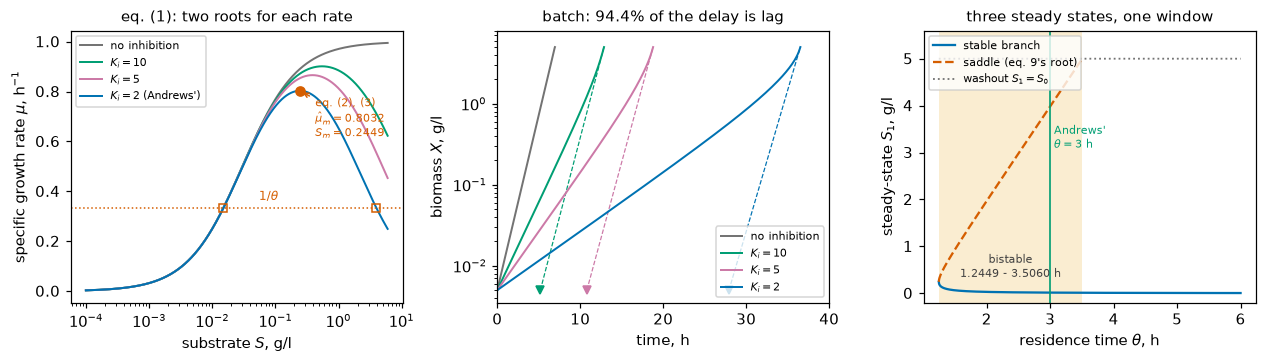
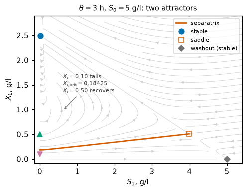
# --------------------------------------------------------------- agreement.json
METRICS = {
    # ---- the inhibition function, eqs. (1)-(3), (6), (11)
    "mu_hat_m_eq2_per_h": MU_HAT_M,
    "S_m_eq3_g_per_l": S_M,
    "eq2_vs_rootfound_max_rel": abs(MU_HAT_M/MU_HAT_M_ROOT - 1),
    "eq3_vs_rootfound_argmax_rel": abs(S_M/S_M_ROOT - 1),
    "theta_washout_h": THETA_W,
    "half_rate_low_root_g_per_l": HALF_LO,
    "half_rate_high_root_g_per_l": HALF_HI,
    "Ks_definition_rel_error": KS_DEF_ERR,
    "Ki_definition_rel_error": KI_DEF_ERR,
    "Ki_min_for_half_rate_defs_g_per_l": KI_MIN_FOR_DEF,
    "rm_as_maximum_overstatement_rel": RM_OVERSTATEMENT,
    # ---- batch: the closed form and Andrews' two stated times
    "batch_time_direct_h": T_DIRECT,
    "batch_time_direct_vs_printed36_rel": REL_36,
    "batch_closedform_vs_lsoda_rel": CF_VS_IVP,
    "batch_time_seeded_h": T_SEED,
    "batch_time_seeded_vs_printed12p5_rel": REL_12P5,
    "seed_readings_raw_spread_rel": SEED_READINGS_SPREAD,
    "seed_reset_vs_increment_rel": SEED_RESET_VS_INC,
    "seed_speedup_factor": SPEEDUP,
    # ---- the batch claim
    "lag_hours_at_Ki2": ROWS[-1]["lag"],
    "lag_share_of_delay_Ki2": LAG_FRAC_2,
    "lag_share_of_delay_Ki5": FRAC[5.0]["lag"],
    "lag_share_of_delay_Ki10": FRAC[10.0]["lag"],
    "lag_share_of_delay_at_Xf1": LAG_SHARE_AT_XF1,
    "peak_growth_rate_drop_rel": MUMAX_DROP,
    "batch_realised_mean_growth_drop_rel": MEAN_MU_DROP,
    "batch_time_ratio_vs_no_inhibition": T_F_RATIO,
    "branch_switch_Ki_g_per_l": KI_SWITCH,
    # ---- the continuous claim
    "steady_S_lower_g_per_l": S_LO,
    "steady_S_upper_g_per_l": S_HI,
    "steady_X_lower_g_per_l": X_LO,
    "steady_X_upper_g_per_l": X_HI,
    "eq9_printed_vs_rootfound_upper_rel": EQ9_VS_ROOT,
    "saddle_positive_eigenvalue_per_h": LAM_SADDLE,
    "washout_eigenvalue_haldane_per_h": LAM_WASHOUT,
    "washout_eigenvalue_monod_per_h": LAM_WASHOUT_MONOD,
    "lower_node_fast_eigenvalue_per_h": LAM_LOWER,
    "theta_transcritical_h": THETA_TRANS,
    "theta_transcritical_two_routes_rel": TRANS_VS_ROOT,
    "monod_vs_haldane_S_shift_rel": S_SHIFT,
    "monod_vs_haldane_X_shift_rel": X_SHIFT,
    "monod_theta_c_h": THETA_C_MONOD,
    # ---- Andrews' six stated outcomes and the thresholds he omits
    "all_six_stated_outcomes_ok": float(ALL_SIX_OK),
    "fig8_direction_ok": float(FIG8_OK),
    "critical_inoculum_g_per_l": X_CRIT,
    "critical_inoculum_two_routes_rel": X_CRIT_TWO_ROUTES,
    "critical_inoculum_S1_init_sensitivity_rel": X_CRIT_SPREAD,
    "critical_step_S0_g_per_l": S0_STEP_CRIT,
    "critical_step_two_routes_rel": STEP_TWO_ROUTES,
    "critical_ramp_duration_h": RAMP_CRIT,
    "andrews_step_margin_rel": STEP_MARGIN,
    "andrews_ramp_margin_rel": RAMP_MARGIN,
    # ---- pymrm
    "pymrm_march_time_step_order": MARCH_ORDER,
    "pymrm_march_richardson_abs_err": MARCH_RICH_ERR,
    "pfr_outlet_grid_order": PFR_ORDER,
    "pfr_last_cell_read_order": PFR_CENTRE_ORDER,
    "pfr_boundary_over_last_cell_err_ratio_ncell800": PFR_BOUNDARY_OVER_CENTRE,
    "pfr_richardson_abs_err": PFR_RICH_ERR,
    "pfr_outlet_X_at_tau3_ncell800_g_per_l": float(pfr_val[-1][1]),
    "pfr_outlet_X_at_tau6_richardson_g_per_l": PFR_X_TAU6,
    "feed_seed_removing_hysteresis_g_per_l": X0_FOLD_CRIT_DOUBLE,
    "feed_seed_fold_two_routes_rel": FOLD_A_FINEST_REL,
    "feed_seed_fold_S_g_per_l": _S_fold,
}

# ---- coverage: GENERATED from the break table's measured moves -------------
# Each break row returned a dict keyed BY METRIC NAME whose values are those
# metrics recomputed under the defect.  Nothing below is a hand-written claim:
# a row covers a metric if, and only if, its recomputed value differs from the
# reported one by more than MOVE_TOL.
COVERAGE, UNKNOWN_KEYS = {}, []
for _label, _got, _note in BREAKS:
    if not isinstance(_got, dict):
        continue
    for _k, _v in _got.items():
        if _k.startswith("_"):
            continue                       # a diagnostic, not a coverage claim
        if _k not in METRICS:
            UNKNOWN_KEYS.append((_label, _k))
            continue
        _base = METRICS[_k]
        # symmetric, so that a metric whose reported value is exactly 0.0 - the
        # transcritical transcription check - still gets a finite move
        _rel = abs(float(_v) - _base)/max(abs(_base), abs(float(_v)), 1e-300)
        if _rel > MOVE_TOL:
            COVERAGE.setdefault(_k, []).append((_label, _rel))
assert not UNKNOWN_KEYS, f"break rows recompute names that are not metrics: {UNKNOWN_KEYS}"

# ---- and the rows must COMPUTE what they return ---------------------------
# A row that returns a TYPED CONSTANT for a metric records a relative move of
# exactly 1.0 whatever the reported value is, so its coverage links cannot fail:
# a hand-written coverage claim wearing the generator's clothes.  This page
# shipped that defect - five literal 0.0s in the lag row, the sole cover of four
# metrics - and the guard below is what makes it unshippable rather than a thing
# each reviewer has to notice again.  It is static and mechanical: it parses each
# row's OWN SOURCE, plus one level of the notebook-defined helpers that row
# names, and rejects any `agreement.json` key bound to a numeric literal, or to a
# local name that is only ever assigned one, in a dict literal, a `dict(...)`
# call or a `d["key"] = ...` assignment.  What it cannot do is say whether the
# expression is the RIGHT one - that is what the measured moves above are for.
import ast
import inspect
import textwrap


def _is_number(node):
    if isinstance(node, ast.Constant):
        return isinstance(node.value, (int, float)) and not isinstance(node.value, bool)
    return (isinstance(node, ast.UnaryOp) and isinstance(node.op, (ast.UAdd, ast.USub))
            and _is_number(node.operand))


def _key_bindings(src):
    """every ("key", value-expression) pair bound anywhere in `src`"""
    tree, out = ast.parse(textwrap.dedent(src)), []
    for n in ast.walk(tree):
        if isinstance(n, ast.Dict):
            out += [(k.value, v) for k, v in zip(n.keys, n.values)
                    if isinstance(k, ast.Constant) and isinstance(k.value, str)]
        elif isinstance(n, ast.Call) and getattr(n.func, "id", "") == "dict":
            out += [(kw.arg, kw.value) for kw in n.keywords if kw.arg]
        elif isinstance(n, ast.Assign):
            for t in n.targets:
                if (isinstance(t, ast.Subscript) and isinstance(t.slice, ast.Constant)
                        and isinstance(t.slice.value, str)):
                    out.append((t.slice.value, n.value))
    return out


def _sources(fn):
    """the row's source, plus that of the notebook functions it names"""
    src = textwrap.dedent(inspect.getsource(fn))
    seen = [src]
    for n in ast.walk(ast.parse(src)):
        if isinstance(n, ast.Name):
            obj = globals().get(n.id)
            if (inspect.isfunction(obj) and getattr(obj, "__module__", "") == "__main__"
                    and obj is not fn):
                try:
                    seen.append(textwrap.dedent(inspect.getsource(obj)))
                except (OSError, TypeError):            # not recoverable: say so
                    seen.append(f"# UNREADABLE SOURCE: {n.id}")
    return seen


def literal_metrics(fn):
    """metrics this row returns as a CONSTANT instead of computing"""
    bad = []
    for src in _sources(fn):
        frozen = {t.id for n in ast.walk(ast.parse(src)) if isinstance(n, ast.Assign)
                  for t in n.targets if isinstance(t, ast.Name) and _is_number(n.value)}
        bad += [k for k, v in _key_bindings(src) if k in METRICS
                and (_is_number(v) or (isinstance(v, ast.Name) and v.id in frozen))]
    return sorted(set(bad))


def _lag_alt_v0():
    """THE NEGATIVE CONTROL: the lag row exactly as this page used to ship it -
    five literals, nothing recomputed, and the only cover of four metrics."""
    return {"lag_hours_at_Ki2": 0.0, "lag_share_of_delay_Ki2": 0.0,
            "lag_share_of_delay_Ki5": 0.0, "lag_share_of_delay_Ki10": 0.0,
            "lag_share_of_delay_at_Xf1": 0.0,
            "_expo_h": np.log(5.0/X_INIT)/float(mu(S_INIT))}


CAUGHT = literal_metrics(_lag_alt_v0)
LITERAL_ROWS = {lbl: bad for lbl, fn in BREAK_FNS for bad in [literal_metrics(fn)] if bad}
print(f"ROWS MUST COMPUTE WHAT THEY RETURN, and it is parsed rather than trusted:"
      f"\n  {len(BREAK_FNS)} rows read; {len(LITERAL_ROWS)} return a metric as a typed"
      f" constant.")
print(f"  the guard's teeth, MEASURED on the row this page used to ship:"
      f" {len(CAUGHT)} of its\n  keys are literal metrics - {CAUGHT}"
      f"\n  (its `_expo_h` is a diagnostic and is correctly not among them).")
assert set(CAUGHT) == {"lag_hours_at_Ki2", "lag_share_of_delay_Ki2",
                       "lag_share_of_delay_Ki5", "lag_share_of_delay_Ki10",
                       "lag_share_of_delay_at_Xf1"}, (
    "the literal guard no longer catches the row it was written for")
assert not LITERAL_ROWS, (
    "break rows returning a metric as a typed constant, so their coverage links"
    f" cannot fail: {LITERAL_ROWS}")

# A metric that no row moves must be named here, individually, with the reason.
STRUCTURAL = {}
uncovered = sorted(set(METRICS) - set(COVERAGE) - set(STRUCTURAL))
print(f"COVERAGE MAP, GENERATED FROM {len(BREAKS)} DEFECT INJECTIONS"
      f" ({len(METRICS)} metrics, move threshold {MOVE_TOL:g} relative):")
for _k in sorted(METRICS):
    if _k in COVERAGE:
        _rows = sorted(COVERAGE[_k], key=lambda r: -r[1])
        print(f"  {_k:44s} {len(_rows)} row(s); strongest {_rows[0][1]:.3e}"
              f"  <- {_rows[0][0]}")
    elif _k in STRUCTURAL:
        print(f"  {_k:44s} STRUCTURAL - {STRUCTURAL[_k]}")
    else:
        print(f"  {_k:44s} UNCOVERED")
assert not uncovered, f"metrics no break row moves and none named structural: {uncovered}"
_moving_rows = {lbl for lbl, got, _ in BREAKS if isinstance(got, dict)
                and any(k in COVERAGE and any(r[0] == lbl for r in COVERAGE[k])
                        for k in got)}
N_BREAK_ROWS, N_MOVING_ROWS = len(BREAKS), len(_moving_rows)
N_COVERAGE_LINKS = sum(len(v) for v in COVERAGE.values())
print(f"\nevery one of the {len(METRICS)} metrics is moved by at least one row;"
      f" {N_MOVING_ROWS} of the\n{N_BREAK_ROWS} rows move a reported metric and"
      f" the map holds {N_COVERAGE_LINKS} measured row-metric links.")

# COVERED IS NOT THE SAME AS COVERED FAR ENOUGH TO MATTER.  check_agreement.py
# compares at 5 %, so a metric whose strongest mover shifts it by less than that
# is one no defect on this page could surface as a regression.  One metric was in
# exactly that position (the S_1(0) sensitivity, moved 0.23 % by its only cover),
# which is why the truncated-sample row exists.  The weakest cover is reported
# here and required to clear CI's comparison tolerance.
CI_REL_TOL = 0.05
WEAKEST_COVER, WEAKEST_METRIC = min((max(r[1] for r in v), k)
                                    for k, v in COVERAGE.items())
print(f"weakest cover on the page: {WEAKEST_COVER:.4%} on {WEAKEST_METRIC}"
      f" - above the {CI_REL_TOL:.0%} at which\ncheck_agreement compares, so every"
      f" metric here is one a defect could surface as a regression.")
assert WEAKEST_COVER > CI_REL_TOL, (
    f"{WEAKEST_METRIC} is moved only {WEAKEST_COVER:.3e} by its strongest row,"
    f" below CI's {CI_REL_TOL} comparison tolerance")
assert N_MOVING_ROWS == N_BREAK_ROWS, (
    "a break row moves no metric: "
    f"{sorted({lbl for lbl, _, _ in BREAKS} - _moving_rows)}")

# quantities PROVED exactly zero: printed, deliberately NOT reported.
EXACT_ZEROS = {
    "sympy eq.(1) - eq.(6)": EQ1_EQ6_RESID,
    "sympy eq.(2) residual": EQ2_RESID,
    "sympy eq.(3) residual": EQ3_RESID,
    "sympy partial-fraction residual": PF_RESID,
    "sympy antiderivative residual": ANTIDERIV_RESID,
    "sympy Andrews eq.(1) - Froment eq.(1.5.2-4)": FROMENT_RESID,
    "sympy Andrews eq.(1) - Rawlings (K_1 = 1/K_i)": RAWLINGS_RESID,
    "eq.(11) - 1/eq.(2)": EQ11_MINUS_INV_EQ2,
    "Monod theta_c mu(S_f) - 1": MONOD_CRIT_IDENTITY,
    "S + X/Y balance, plug-flow cells": PFR_BALANCE_CELLS,
}
print("\nPROVED EXACTLY ZERO - printed, NOT reported (CI compares above 1e-12 at 5 %,"
      "\nand a symbolic zero is a proof, not a measurement):")
for k, v in EXACT_ZEROS.items():
    print(f"  {k:52s} = {v}")
assert not (set(EXACT_ZEROS) & set(METRICS)), "an exact zero leaked into METRICS"
assert float(EQ11_MINUS_INV_EQ2) == 0.0
assert PFR_BALANCE_CELLS < 1e-12

# Four reported residuals are TRANSCRIPTION CHECKS, not independent
# computations: they are zero by algebra whenever the equations are copied
# correctly, so the only thing that can move them is a mis-transcription - and
# the break table mis-transcribes each one to show it does.
TRANSCRIPTION_CHECKS = {
    "eq2_vs_rootfound_max_rel":
        "eq. (2) against the root-found maximum of eq. (6): the same extremum by"
        " two expressions, equal by algebra",
    "eq3_vs_rootfound_argmax_rel":
        "eq. (3) against the Brent root of the analytic dmu/dS: equal by algebra",
    "eq9_printed_vs_rootfound_upper_rel":
        "eq. (9) as printed against the Brent root of mu(S) = 1/theta: the same"
        " quadratic solved two ways",
    "theta_transcritical_two_routes_rel":
        "1/mu(S_0) against a Brent root of eq. (9) at S_+ = S_0: the same"
        " equation rearranged, so it agrees to 0.0 exactly",
}
assert set(TRANSCRIPTION_CHECKS) <= set(METRICS)
print(f"\n{len(TRANSCRIPTION_CHECKS)} of the {len(METRICS)} metrics are"
      f" TRANSCRIPTION CHECKS rather than second computations -\nzero by algebra"
      f" when the copying is right, and each has a break row that mis-transcribes"
      f"\nexactly one term of the equation it checks:")
for k, why in TRANSCRIPTION_CHECKS.items():
    print(f"  {k:38s} = {METRICS[k]:.3e}   {why}")

# Metrics that sit below CI's ABS_FLOOR are OUTSIDE the regression suite while
# both sides stay under it.  Each one is named here with an ABOVE-FLOOR
# COMPANION that carries the same physics and is compared.
ABS_FLOOR = 1e-12
BELOW_FLOOR_COMPANION = {
    "eq2_vs_rootfound_max_rel": "mu_hat_m_eq2_per_h",
    "eq3_vs_rootfound_argmax_rel": "S_m_eq3_g_per_l",
    "eq9_printed_vs_rootfound_upper_rel": "steady_S_upper_g_per_l",
    "theta_transcritical_two_routes_rel": "theta_transcritical_h",
    "critical_step_two_routes_rel": "critical_step_S0_g_per_l",
    "critical_inoculum_two_routes_rel": "critical_inoculum_g_per_l",
    "feed_seed_fold_two_routes_rel": "feed_seed_removing_hysteresis_g_per_l",
}
below = {k: v for k, v in METRICS.items() if abs(v) < ABS_FLOOR}
unnamed = set(below) - set(BELOW_FLOOR_COMPANION)
assert not unnamed, f"metrics below ABS_FLOOR with no companion named: {unnamed}"
assert set(BELOW_FLOOR_COMPANION) <= set(METRICS)
for k, comp in BELOW_FLOOR_COMPANION.items():
    assert abs(METRICS[comp]) > ABS_FLOOR, f"companion {comp} is itself below floor"
N_BELOW_FLOOR = len(below)
print(f"\nbelow CI's ABS_FLOOR = {ABS_FLOOR:g}, so outside the regression suite"
      f" ({N_BELOW_FLOOR} of {len(METRICS)}):")
for k in BELOW_FLOOR_COMPANION:
    mark = "BELOW" if k in below else "above"
    print(f"  {mark}  {k:38s} = {METRICS[k]:.3e}"
          f"   companion {BELOW_FLOOR_COMPANION[k]}"
          f" = {METRICS[BELOW_FLOOR_COMPANION[k]]:.6g}")

# ---- the second computations, counted and ranged by the code ---------------
SECOND_ROUTES = {
    "batch time to 5 g/l, closed form vs LSODA": CF_VS_IVP,
    "upper steady state, eq. (9) vs Brent [transcription]": EQ9_VS_ROOT,
    "transcritical theta, 1/mu(S_0) vs Brent [transcription]": TRANS_VS_ROOT,
    "critical inoculum, bisection vs stable manifold": X_CRIT_TWO_ROUTES,
    "critical step, bisection vs separatrix side test": STEP_TWO_ROUTES,
    "X_0 fold, root count vs double root": FOLD_A_FINEST_REL,
}
N_SECOND_ROUTES = len(SECOND_ROUTES)
N_INDEPENDENT_ROUTES = N_SECOND_ROUTES - len(
    [k for k in SECOND_ROUTES if "transcription" in k])
SECOND_ROUTE_MAX = max(SECOND_ROUTES.values())
SECOND_ROUTE_MIN = min(SECOND_ROUTES.values())
print(f"\n{N_SECOND_ROUTES} quantities are computed twice"
      f" ({N_INDEPENDENT_ROUTES} by genuinely independent routes, the other"
      f" {N_SECOND_ROUTES - N_INDEPENDENT_ROUTES}\nby a second transcription of"
      f" the same algebra), agreeing between {SECOND_ROUTE_MIN:.1e} and"
      f" {SECOND_ROUTE_MAX:.1e}:")
for k, v in SECOND_ROUTES.items():
    print(f"  {v:.3e}   {k}")

print()
report_agreement(PAGE, METRICS)
ROWS MUST COMPUTE WHAT THEY RETURN, and it is parsed rather than trusted:
24 rows read; 0 return a metric as a typed constant.
the guard's teeth, MEASURED on the row this page used to ship: 5 of its
keys are literal metrics - ['lag_hours_at_Ki2', 'lag_share_of_delay_Ki10', 'lag_share_of_delay_Ki2', 'lag_share_of_delay_Ki5', 'lag_share_of_delay_at_Xf1']
(its `_expo_h` is a diagnostic and is correctly not among them).
COVERAGE MAP, GENERATED FROM 24 DEFECT INJECTIONS (63 metrics, move threshold 1e-06 relative):
Ki_definition_rel_error 2 row(s); strongest 1.000e+00 <- K_i -> inf (Monod)
Ki_min_for_half_rate_defs_g_per_l 1 row(s); strongest 5.000e-01 <- K_s 0.03 -> 0.015
Ks_definition_rel_error 2 row(s); strongest 9.320e-01 <- K_i -> inf (Monod)
S_m_eq3_g_per_l 3 row(s); strongest 1.000e+00 <- K_i -> inf (Monod)
all_six_stated_outcomes_ok 2 row(s); strongest 1.000e+00 <- theta 3 -> 4 h (above 1/mu(S_0))
andrews_ramp_margin_rel 1 row(s); strongest 1.370e+00 <- muhat 1.0 -> 0.9
andrews_step_margin_rel 2 row(s); strongest 1.703e+00 <- S_0 5 -> 7 g/l (still bistable)
batch_closedform_vs_lsoda_rel 1 row(s); strongest 1.000e+00 <- closed form with the (S_f - S_i)/K_i term dropped
batch_realised_mean_growth_drop_rel 1 row(s); strongest 1.000e+00 <- K_i -> inf (Monod)
batch_time_direct_h 4 row(s); strongest 8.098e-01 <- K_i -> inf (Monod)
batch_time_direct_vs_printed36_rel 4 row(s); strongest 1.018e+00 <- K_i -> inf (Monod)
batch_time_ratio_vs_no_inhibition 1 row(s); strongest 8.098e-01 <- K_i -> inf (Monod)
batch_time_seeded_h 4 row(s); strongest 4.218e-01 <- K_i -> inf (Monod)
batch_time_seeded_vs_printed12p5_rel 4 row(s); strongest 1.103e+00 <- muhat 1.0 -> 0.9
branch_switch_Ki_g_per_l 1 row(s); strongest 5.000e-01 <- K_s 0.03 -> 0.015
critical_inoculum_S1_init_sensitivity_rel 2 row(s); strongest 9.219e-01 <- S_1(0) sensitivity over a truncated sample
critical_inoculum_g_per_l 3 row(s); strongest 6.659e-01 <- S_0 5 -> 7 g/l (still bistable)
critical_inoculum_two_routes_rel 2 row(s); strongest 1.000e+00 <- outcome classified at t = 50 h instead of on an event
critical_ramp_duration_h 1 row(s); strongest 4.737e-01 <- muhat 1.0 -> 0.9
critical_step_S0_g_per_l 2 row(s); strongest 2.309e-01 <- S_0 5 -> 7 g/l (still bistable)
critical_step_two_routes_rel 1 row(s); strongest 1.000e+00 <- separatrix route B queried at the wrong substrate
eq2_vs_rootfound_max_rel 1 row(s); strongest 1.000e+00 <- eq. (2) transcribed without the 2, eq. (3) without the square root
eq3_vs_rootfound_argmax_rel 1 row(s); strongest 1.000e+00 <- eq. (2) transcribed without the 2, eq. (3) without the square root
eq9_printed_vs_rootfound_upper_rel 1 row(s); strongest 1.000e+00 <- eq. (9) transcribed with 4 K_s K_i as 4 K_s
feed_seed_fold_S_g_per_l 2 row(s); strongest 1.821e-01 <- S_0 5 -> 7 g/l (still bistable)
feed_seed_fold_two_routes_rel 1 row(s); strongest 1.000e+00 <- the X_0 fold reported from the root COUNT at ngrid 1501
feed_seed_removing_hysteresis_g_per_l 3 row(s); strongest 8.867e-01 <- S_0 5 -> 7 g/l (still bistable)
fig8_direction_ok 2 row(s); strongest 1.000e+00 <- theta 3 -> 4 h (above 1/mu(S_0))
half_rate_high_root_g_per_l 2 row(s); strongest 1.000e+00 <- K_i -> inf (Monod)
half_rate_low_root_g_per_l 2 row(s); strongest 5.039e-01 <- K_s 0.03 -> 0.015
lag_hours_at_Ki2 2 row(s); strongest 1.000e+00 <- K_i -> inf (Monod)
lag_share_of_delay_Ki10 1 row(s); strongest 1.000e+00 <- lag tangent at t=0, not at the peak
lag_share_of_delay_Ki2 1 row(s); strongest 1.000e+00 <- lag tangent at t=0, not at the peak
lag_share_of_delay_Ki5 1 row(s); strongest 1.000e+00 <- lag tangent at t=0, not at the peak
lag_share_of_delay_at_Xf1 1 row(s); strongest 1.000e+00 <- lag tangent at t=0, not at the peak
lower_node_fast_eigenvalue_per_h 6 row(s); strongest 9.954e-01 <- operate at eq.(9)'s printed root
monod_theta_c_h 3 row(s); strongest 1.000e-01 <- muhat 1.0 -> 0.9
monod_vs_haldane_S_shift_rel 5 row(s); strongest 1.000e+00 <- K_i -> inf (Monod)
monod_vs_haldane_X_shift_rel 5 row(s); strongest 1.000e+00 <- K_i -> inf (Monod)
mu_hat_m_eq2_per_h 4 row(s); strongest 1.968e-01 <- K_i -> inf (Monod)
peak_growth_rate_drop_rel 2 row(s); strongest 1.015e+00 <- K_i -> inf (Monod)
pfr_boundary_over_last_cell_err_ratio_ncell800 2 row(s); strongest 2.439e-01 <- construct_div nu=1 (cylindrical)
pfr_last_cell_read_order 2 row(s); strongest 1.000e+00 <- construct_div nu=1 (cylindrical)
pfr_outlet_X_at_tau3_ncell800_g_per_l 3 row(s); strongest 1.000e+00 <- inlet bc zero-gradient not Dirichlet
pfr_outlet_X_at_tau6_richardson_g_per_l 1 row(s); strongest 1.000e+00 <- construct_div nu=1 (cylindrical)
pfr_outlet_grid_order 3 row(s); strongest 1.000e+00 <- construct_div nu=1 (cylindrical)
pfr_richardson_abs_err 3 row(s); strongest 1.000e+00 <- construct_div nu=1 (cylindrical)
pymrm_march_richardson_abs_err 1 row(s); strongest 1.000e+00 <- marcher: -c/theta dropped from the constant operator
pymrm_march_time_step_order 1 row(s); strongest 1.000e+00 <- marcher: -c/theta dropped from the constant operator
rm_as_maximum_overstatement_rel 3 row(s); strongest 1.000e+00 <- K_i -> inf (Monod)
saddle_positive_eigenvalue_per_h 3 row(s); strongest 6.633e-01 <- S_0 5 -> 7 g/l (still bistable)
seed_readings_raw_spread_rel 1 row(s); strongest 9.242e-01 <- K_i -> inf (Monod)
seed_reset_vs_increment_rel 1 row(s); strongest 1.168e+00 <- K_i -> inf (Monod)
seed_speedup_factor 3 row(s); strongest 6.710e-01 <- K_i -> inf (Monod)
steady_S_lower_g_per_l 5 row(s); strongest 9.962e-01 <- operate at eq.(9)'s printed root
steady_S_upper_g_per_l 2 row(s); strongest 1.512e-01 <- muhat 1.0 -> 0.9
steady_X_lower_g_per_l 7 row(s); strongest 7.964e-01 <- operate at eq.(9)'s printed root
steady_X_upper_g_per_l 4 row(s); strongest 6.633e-01 <- S_0 5 -> 7 g/l (still bistable)
theta_transcritical_h 5 row(s); strongest 7.131e-01 <- K_i -> inf (Monod)
theta_transcritical_two_routes_rel 1 row(s); strongest 1.000e+00 <- eq. (9) transcribed with 4 K_s K_i as 4 K_s
theta_washout_h 3 row(s); strongest 1.968e-01 <- K_i -> inf (Monod)
washout_eigenvalue_haldane_per_h 6 row(s); strongest 1.739e+00 <- S_0 5 -> 3 g/l (below the bistable range)
washout_eigenvalue_monod_per_h 4 row(s); strongest 1.505e-01 <- muhat 1.0 -> 0.9
every one of the 63 metrics is moved by at least one row; 24 of the
24 rows move a reported metric and the map holds 154 measured row-metric links.
weakest cover on the page: 10.0000% on monod_theta_c_h - above the 5% at which
check_agreement compares, so every metric here is one a defect could surface as a regression.
PROVED EXACTLY ZERO - printed, NOT reported (CI compares above 1e-12 at 5 %,
and a symbolic zero is a proof, not a measurement):
sympy eq.(1) - eq.(6) = 0
sympy eq.(2) residual = 0
sympy eq.(3) residual = 0
sympy partial-fraction residual = 0
sympy antiderivative residual = 0
sympy Andrews eq.(1) - Froment eq.(1.5.2-4) = 0
sympy Andrews eq.(1) - Rawlings (K_1 = 1/K_i) = 0
eq.(11) - 1/eq.(2) = 0.0
Monod theta_c mu(S_f) - 1 = 1.1102230246251565e-16
S + X/Y balance, plug-flow cells = 6.661338147750939e-16
4 of the 63 metrics are TRANSCRIPTION CHECKS rather than second computations -
zero by algebra when the copying is right, and each has a break row that mis-transcribes
exactly one term of the equation it checks:
eq2_vs_rootfound_max_rel = 2.220e-16 eq. (2) against the root-found maximum of eq. (6): the same extremum by two expressions, equal by algebra
eq3_vs_rootfound_argmax_rel = 2.220e-16 eq. (3) against the Brent root of the analytic dmu/dS: equal by algebra
eq9_printed_vs_rootfound_upper_rel = 1.110e-16 eq. (9) as printed against the Brent root of mu(S) = 1/theta: the same quadratic solved two ways
theta_transcritical_two_routes_rel = 0.000e+00 1/mu(S_0) against a Brent root of eq. (9) at S_+ = S_0: the same equation rearranged, so it agrees to 0.0 exactly
below CI's ABS_FLOOR = 1e-12, so outside the regression suite (5 of 63):
BELOW eq2_vs_rootfound_max_rel = 2.220e-16 companion mu_hat_m_eq2_per_h = 0.803246
BELOW eq3_vs_rootfound_argmax_rel = 2.220e-16 companion S_m_eq3_g_per_l = 0.244949
BELOW eq9_printed_vs_rootfound_upper_rel = 1.110e-16 companion steady_S_upper_g_per_l = 3.98494
BELOW theta_transcritical_two_routes_rel = 0.000e+00 companion theta_transcritical_h = 3.506
BELOW critical_step_two_routes_rel = 8.060e-14 companion critical_step_S0_g_per_l = 17.2876
above critical_inoculum_two_routes_rel = 2.351e-12 companion critical_inoculum_g_per_l = 0.184247
above feed_seed_fold_two_routes_rel = 1.183e-09 companion feed_seed_removing_hysteresis_g_per_l = 0.0213935
6 quantities are computed twice (4 by genuinely independent routes, the other 2
by a second transcription of the same algebra), agreeing between 0.0e+00 and 1.2e-09:
6.682e-12 batch time to 5 g/l, closed form vs LSODA
1.110e-16 upper steady state, eq. (9) vs Brent [transcription]
0.000e+00 transcritical theta, 1/mu(S_0) vs Brent [transcription]
2.351e-12 critical inoculum, bisection vs stable manifold
8.060e-14 critical step, bisection vs separatrix side test
1.183e-09 X_0 fold, root count vs double root
Agreement metrics for J4.2-andrews-substrate-inhibition:
mu_hat_m_eq2_per_h = 0.80325
S_m_eq3_g_per_l = 0.24495
eq2_vs_rootfound_max_rel = 2.2204e-16
eq3_vs_rootfound_argmax_rel = 2.2204e-16
theta_washout_h = 1.2449
half_rate_low_root_g_per_l = 0.030464
half_rate_high_root_g_per_l = 1.9695
Ks_definition_rel_error = 0.015468
Ki_definition_rel_error = -0.015232
Ki_min_for_half_rate_defs_g_per_l = 0.12
rm_as_maximum_overstatement_rel = 0.24495
batch_time_direct_h = 36.527
batch_time_direct_vs_printed36_rel = 0.014652
batch_closedform_vs_lsoda_rel = 6.682e-12
batch_time_seeded_h = 12.372
batch_time_seeded_vs_printed12p5_rel = -0.010272
seed_readings_raw_spread_rel = 0.11544
seed_reset_vs_increment_rel = -0.00041854
seed_speedup_factor = 2.9525
lag_hours_at_Ki2 = 27.922
lag_share_of_delay_Ki2 = 0.94401
lag_share_of_delay_Ki5 = 0.91249
lag_share_of_delay_Ki10 = 0.87779
lag_share_of_delay_at_Xf1 = 1.094
peak_growth_rate_drop_rel = -0.19434
batch_realised_mean_growth_drop_rel = -0.80976
batch_time_ratio_vs_no_inhibition = 5.2564
branch_switch_Ki_g_per_l = 3333.3
steady_S_lower_g_per_l = 0.015057
steady_S_upper_g_per_l = 3.9849
steady_X_lower_g_per_l = 2.4925
steady_X_upper_g_per_l = 0.50753
eq9_printed_vs_rootfound_upper_rel = 1.1102e-16
saddle_positive_eigenvalue_per_h = 0.056179
washout_eigenvalue_haldane_per_h = -0.048108
washout_eigenvalue_monod_per_h = 0.6607
lower_node_fast_eigenvalue_per_h = -73.019
theta_transcritical_h = 3.506
theta_transcritical_two_routes_rel = 0
monod_vs_haldane_S_shift_rel = 0.0037784
monod_vs_haldane_X_shift_rel = -1.1369e-05
monod_theta_c_h = 1.006
all_six_stated_outcomes_ok = 1
fig8_direction_ok = 1
critical_inoculum_g_per_l = 0.18425
critical_inoculum_two_routes_rel = 2.3506e-12
critical_inoculum_S1_init_sensitivity_rel = 0.05212
critical_step_S0_g_per_l = 17.288
critical_step_two_routes_rel = 8.0602e-14
critical_ramp_duration_h = 0.87207
andrews_step_margin_rel = 0.1569
andrews_ramp_margin_rel = 0.1467
pymrm_march_time_step_order = 1.0021
pymrm_march_richardson_abs_err = 1.7021e-07
pfr_outlet_grid_order = 1.0011
pfr_last_cell_read_order = 1.0013
pfr_boundary_over_last_cell_err_ratio_ncell800 = 1.3226
pfr_richardson_abs_err = 4.2543e-07
pfr_outlet_X_at_tau3_ncell800_g_per_l = 0.23891
pfr_outlet_X_at_tau6_richardson_g_per_l = 0.60765
feed_seed_removing_hysteresis_g_per_l = 0.021393
feed_seed_fold_two_routes_rel = 1.1833e-09
feed_seed_fold_S_g_per_l = 4.4926{'page': 'J4.2-andrews-substrate-inhibition',
'metrics': {'mu_hat_m_eq2_per_h': 0.8032457720443428,
'S_m_eq3_g_per_l': 0.2449489742783178,
'eq2_vs_rootfound_max_rel': 2.220446049250313e-16,
'eq3_vs_rootfound_argmax_rel': 2.220446049250313e-16,
'theta_washout_h': 1.2449489742783177,
'half_rate_low_root_g_per_l': 0.030464028516734243,
'half_rate_high_root_g_per_l': 1.9695359714832659,
'Ks_definition_rel_error': 0.0154676172244748,
'Ki_definition_rel_error': -0.015232014258367066,
'Ki_min_for_half_rate_defs_g_per_l': 0.12,
'rm_as_maximum_overstatement_rel': 0.24494897427831774,
'batch_time_direct_h': 36.52747557683508,
'batch_time_direct_vs_printed36_rel': 0.014652099356530002,
'batch_closedform_vs_lsoda_rel': 6.681988296008967e-12,
'batch_time_seeded_h': 12.371597482794177,
'batch_time_seeded_vs_printed12p5_rel': -0.010272201376465801,
'seed_readings_raw_spread_rel': 0.11544189992147746,
'seed_reset_vs_increment_rel': -0.0004185386770062527,
'seed_speedup_factor': 2.9525269980401267,
'lag_hours_at_Ki2': 27.922318494599278,
'lag_share_of_delay_Ki2': 0.9440131506118717,
'lag_share_of_delay_Ki5': 0.9124871582573425,
'lag_share_of_delay_Ki10': 0.8777879980628407,
'lag_share_of_delay_at_Xf1': 1.0940027701847395,
'peak_growth_rate_drop_rel': -0.19434449063149173,
'batch_realised_mean_growth_drop_rel': -0.8097552514689615,
'batch_time_ratio_vs_no_inhibition': 5.256386879119819,
'branch_switch_Ki_g_per_l': 3333.3333333333335,
'steady_S_lower_g_per_l': 0.015056675872079211,
'steady_S_upper_g_per_l': 3.9849433241279213,
'steady_X_lower_g_per_l': 2.49247166206396,
'steady_X_upper_g_per_l': 0.5075283379360394,
'eq9_printed_vs_rootfound_upper_rel': 1.1102230246251565e-16,
'saddle_positive_eigenvalue_per_h': 0.056178966354689996,
'washout_eigenvalue_haldane_per_h': -0.048108005324206116,
'washout_eigenvalue_monod_per_h': 0.6607024519549369,
'lower_node_fast_eigenvalue_per_h': -73.01914192931764,
'theta_transcritical_h': 3.5060000000000002,
'theta_transcritical_two_routes_rel': 0.0,
'monod_vs_haldane_S_shift_rel': 0.00377839147194745,
'monod_vs_haldane_X_shift_rel': -1.1369282262771176e-05,
'monod_theta_c_h': 1.006,
'all_six_stated_outcomes_ok': 1.0,
'fig8_direction_ok': 1.0,
'critical_inoculum_g_per_l': 0.18424664213673553,
'critical_inoculum_two_routes_rel': 2.3505641877363814e-12,
'critical_inoculum_S1_init_sensitivity_rel': 0.05211954741897018,
'critical_step_S0_g_per_l': 17.287597871124817,
'critical_step_two_routes_rel': 8.060219158778636e-14,
'critical_ramp_duration_h': 0.8720667988003954,
'andrews_step_margin_rel': 0.15689872873579858,
'andrews_ramp_margin_rel': 0.14670114878308405,
'pymrm_march_time_step_order': 1.0021309950485744,
'pymrm_march_richardson_abs_err': 1.702079659661626e-07,
'pfr_outlet_grid_order': 1.0011321846858463,
'pfr_last_cell_read_order': 1.001305959559354,
'pfr_boundary_over_last_cell_err_ratio_ncell800': 1.322621457072709,
'pfr_richardson_abs_err': 4.254326150925653e-07,
'pfr_outlet_X_at_tau3_ncell800_g_per_l': 0.23890743618872498,
'pfr_outlet_X_at_tau6_richardson_g_per_l': 0.6076462145033377,
'feed_seed_removing_hysteresis_g_per_l': 0.021393476490798143,
'feed_seed_fold_two_routes_rel': 1.1833438673392038e-09,
'feed_seed_fold_S_g_per_l': 4.492568064568628}}# ---------------------------------------------------------------- prose sweep
# Every number written in the markdown of this notebook, in meta.yaml, in
# README.md and in models_entry.yaml is checked here against the live
# computation. The notebook FAILS TO EXECUTE if any of them drifts.
CLAIMS = [
("mu_hat_m", 0.803246, MU_HAT_M, 5e-7),
("S_m", 0.244949, S_M, 5e-7),
("theta_w", 1.244949, THETA_W, 5e-7),
("theta_transcritical", 3.506000, THETA_TRANS, 5e-7),
("half-rate low root", 0.0304640, HALF_LO, 5e-8),
("half-rate high root", 1.969536, HALF_HI, 5e-7),
("K_s definition error", 0.015468, KS_DEF_ERR, 5e-7),
("K_i definition error", -0.015232, KI_DEF_ERR, 5e-7),
("K_i >= 4 K_s", 0.12, KI_MIN_FOR_DEF, 1e-12),
("t_direct", 36.527476, T_DIRECT, 5e-7),
("t_direct vs printed 36", 0.014652, REL_36, 5e-7),
("t_seed increment (reported)", 12.371597, T_SEED, 5e-7),
("t_seed vs printed 12.5", -0.010272, REL_12P5, 5e-7),
("t_seed reset", 12.366419, T_SEED_RESET, 5e-7),
("t_seed reset vs 12.5", -0.010686, REL_12P5_RESET, 5e-7),
("t_seed ladder", 13.794022, T_SEED_LADDER, 5e-7),
("t_seed ladder vs 12.5", 0.103522, REL_12P5_LADDER, 5e-7),
("raw spread of the three readings", 0.115442, SEED_READINGS_SPREAD, 5e-7),
("reset vs increment", -0.000419, SEED_RESET_VS_INC, 5e-7),
("speedup", 2.9525, SPEEDUP, 5e-5),
("cycles", 6, N_CYCLES, 0),
("first cycle", 9.770815, CYCLE_T[0], 5e-7),
("remaining cycles", 2.600783, sum(CYCLE_T[1:]), 5e-7),
("t_f no inhibition", 6.949160, NO_INHIB["t_f"], 5e-7),
("t_f at K_i=2", 36.527476, ROWS[-1]["t_f"], 5e-7),
("t_f ratio", 5.256387, T_F_RATIO, 5e-7),
("delta t_f at K_i=2", 29.578315, DT_F_2, 5e-7),
("lag hours at K_i=2", 27.922318, ROWS[-1]["lag"], 5e-7),
("lag share K_i=2", 0.944013, LAG_FRAC_2, 5e-7),
("expo share K_i=2", 0.056505, FRAC[2.0]["expo"], 5e-7),
("tail share K_i=2", -0.000518, FRAC[2.0]["tail"], 5e-7),
("lag share K_i=5", 0.912487, FRAC[5.0]["lag"], 5e-7),
("lag share K_i=10", 0.877788, FRAC[10.0]["lag"], 5e-7),
("lag share at X_f = 1 g/l", 1.094003, LAG_SHARE_AT_XF1, 5e-7),
("lag share at X_f = 0.5 g/l", 1.238027, SHARE_VS_XF[0.5]["lag"], 5e-7),
("batch asymptote Y a", 5.005, YIELD*(S_INIT + X_INIT/YIELD), 1e-12),
("peak mu no inhibition", 0.997009, NO_INHIB["mu_max"], 5e-7),
("peak mu at K_i=2", 0.803246, ROWS[-1]["mu_max"], 5e-7),
("peak mu drop", -0.194344, MUMAX_DROP, 5e-7),
("t_peak at K_i=2", 36.492522, ROWS[-1]["t_peak"], 5e-7),
("t_peak as a fraction of t_f", 0.999043, T_PEAK_FRACTION, 5e-7),
("expo term at K_i=2", 8.599803, ROWS[-1]["expo"], 5e-7),
("time above half the peak rate", 0.638869, T_ABOVE_HALF, 5e-7),
("fraction above half the peak", 0.017490, FRAC_ABOVE_HALF, 5e-7),
("realised mean mu, no inhibition", 0.994042, MEAN_MU_NOINH, 5e-7),
("realised mean mu at K_i=2", 0.189111, MEAN_MU_KI2, 5e-7),
("realised mean mu drop", -0.809755, MEAN_MU_DROP, 5e-7),
("X at t = lag", 0.573354, X_AT_LAG, 5e-7),
("fold rise during the lag", 114.6707, LAG_FOLD_RISE, 5e-5),
("half-rate low root, K_i=1.0", 0.030958, HALF_TABLE[1]["low"], 5e-7),
("half-rate high root, K_i=1.0", 0.969042, HALF_TABLE[1]["high"], 5e-7),
("K_s definition error, K_i=1.0", 0.031947, HALF_TABLE[1]["ks_err"], 5e-7),
("K_i definition error, K_i=1.0", -0.030958, HALF_TABLE[1]["ki_err"], 5e-7),
("half-rate low root, K_i=0.5", 0.032055, HALF_TABLE[2]["low"], 5e-7),
("half-rate high root, K_i=0.5", 0.467945, HALF_TABLE[2]["high"], 5e-7),
("K_s definition error, K_i=0.5", 0.068502, KS_DEF_ERR_FIG1, 5e-7),
("K_i definition error, K_i=0.5", -0.064110, KI_DEF_ERR_FIG1, 5e-7),
("S lower", 0.0150567, S_LO, 5e-8),
("S upper", 3.984943, S_HI, 5e-7),
("X lower", 2.492472, X_LO, 5e-7),
("X upper", 0.507528, X_HI, 5e-7),
("eq.(9) root over the lower root", 264.66, S1_EQ9/S_LO, 5e-3),
("saddle eigenvalue", 0.0561790, LAM_SADDLE, 5e-8),
("washout eig Haldane", -0.0481080, LAM_WASHOUT, 5e-8),
("washout eig Monod", 0.660702, LAM_WASHOUT_MONOD, 5e-7),
("lower node fast eig", -73.019142, LAM_LOWER, 5e-5),
("S shift Monod->Haldane", 0.003778, S_SHIFT, 5e-6),
("X shift Monod->Haldane", -0.000011369, X_SHIFT, 5e-9),
("r_m overstatement", 0.244949, RM_OVERSTATEMENT, 5e-7),
("X_crit", 0.1842466, X_CRIT, 5e-8),
("X_crit two routes", 0.0, X_CRIT_TWO_ROUTES, 2e-11),
("X_crit lowest over S_1(0)", 0.1840000, min(SENS.values()), 5e-8),
("X_crit highest over S_1(0)", 0.1935900, max(SENS.values()), 5e-8),
("X_crit spread, [0, 0.2]", 0.052120, X_CRIT_SPREAD, 5e-6),
("X_crit spread, [0, 0.05]", 0.004071, X_CRIT_SPREAD_NARROW, 5e-6),
("X_i=0.10 below crit", -0.457, 0.10/X_CRIT - 1, 5e-4),
("X_i=0.50 above crit", 1.714, 0.50/X_CRIT - 1, 5e-4),
("critical step", 17.28760, S0_STEP_CRIT, 5e-6),
("critical step two routes", 0.0, STEP_TWO_ROUTES, 2e-12),
("step margin", 0.157, STEP_MARGIN, 5e-4),
("critical ramp", 0.8720668, RAMP_CRIT, 5e-8),
("ramp margin", 0.1467, RAMP_MARGIN, 5e-5),
("Monod theta_c", 1.006, THETA_C_MONOD, 5e-4),
("X_0 killing the fold", 0.0213935, X0_FOLD_CRIT_DOUBLE, 5e-8),
("X_0 fold as % of X_1", 0.008583, X0_FOLD_CRIT_DOUBLE/X_LO, 5e-7),
("fold route A, ngrid 1501", 0.0049, abs(FOLD_A_REFINE[1501]
/X0_FOLD_CRIT_DOUBLE - 1), 5e-5),
("fold route A, ngrid 6001", 0.0000053, abs(FOLD_A_REFINE[6001]
/X0_FOLD_CRIT_DOUBLE - 1), 5e-8),
("fold route A, ngrid 96001", 0.0000000012, FOLD_A_FINEST_REL, 5e-11),
("X_crit two routes (table)", 0.0, X_CRIT_TWO_ROUTES, 2.5e-12),
("step two routes (table)", 0.0, STEP_TWO_ROUTES, 8.2e-14),
("closed form vs LSODA", 0.0, CF_VS_IVP, 1e-11),
("LSODA batch time", 36.527476, T_DIRECT_IVP, 5e-7),
("plug-flow boundary read order", 1.0011, PFR_ORDER, 5e-5),
("plug-flow last-cell read order", 1.0013, PFR_CENTRE_ORDER, 5e-5),
("boundary over last-cell error", 1.3226, PFR_BOUNDARY_OVER_CENTRE, 5e-5),
("boundary over last-cell, ncell 100", 1.3215, PFR_B["err"][0]/PFR_C["err"][0], 5e-5),
("marcher time-step order", 1.0021, MARCH_ORDER, 5e-5),
("PFR outlet X at tau 3, ncell 800", 0.2389074, float(pfr_val[-1][1]), 5e-8),
("PFR outlet X at tau 6, Richardson", 0.6076462, PFR_X_TAU6, 5e-8),
("PFR outlet X at tau 6, ncell 1200", 0.6086420, PFR_X_TAU6_GRID, 5e-8),
("PFR tau 6 grid value vs converged", 0.001637, PFR_TAU6_GRID_ERR, 5e-6),
]
bad = [(n, w, g) for n, w, g, t in CLAIMS if abs(float(g) - w) > t]
assert not bad, "PROSE DRIFT:\n" + "\n".join(
f" {n}: page says {w!r}, live value {float(g)!r}" for n, w, g in bad)
print(f"{len(CLAIMS)} prose/metadata values checked against the live"
f" computation: all agree.")
# ---- mechanical sweep of the metadata FILES ------------------------------
# Every number written with FIVE OR MORE DECIMAL PLACES in meta.yaml,
# README.md, models_entry.yaml and the data sidecar must match some live value
# to HALF AN ULP OF ITS OWN PRINTED DIGITS. Five decimals rather than four is
# deliberate: it excludes the DOI (10.1002/...) without an exception list.
# The sweep then MEASURES ITS OWN TEETH by corrupting the last printed digit of
# every token it found and reporting how many of those corruptions it rejects.
import re
LIVE = set()
for _v in METRICS.values():
LIVE.add(float(_v))
for _v in (list(FRAC.values())):
LIVE.update(float(x) for x in _v.values())
for _r in ROWS:
LIVE.update(float(_r[k]) for k in ("mu_max", "S_m", "t_peak", "lag", "expo",
"tail", "t_f"))
LIVE.update([float(x) for x in CYCLE_T])
LIVE.update([sum(CYCLE_T[1:]), T_SEED_RESET, REL_12P5_RESET, T_SEED_LADDER,
REL_12P5_LADDER, SEED_READINGS_SPREAD, SEED_RESET_VS_INC,
X0_FOLD_CRIT, X0_FOLD_CRIT_DOUBLE, X0_FOLD_CRIT_DOUBLE/X_LO,
_S_fold, S1_EQ9, S1_EQ9_MINUS, S_MONOD, X_MONOD, D_C_MONOD,
KI_SWITCH, MU_HAT_M_ROOT, S_M_ROOT, HALF_LO_BRENT, HALF_HI_BRENT,
THETA_TRANS_ROOT, X_CRIT_MANIFOLD, S0_STEP_CRIT_SEP, PFR_X_MAX,
0.10/X_CRIT - 1, 0.50/X_CRIT - 1, T_DIRECT_IVP,
T_PEAK_FRACTION, MEAN_MU_KI2, MEAN_MU_NOINH, MEAN_MU_DROP,
X_AT_LAG, LAG_FOLD_RISE, T_ABOVE_HALF, FRAC_ABOVE_HALF,
X_CRIT_SPREAD_NARROW, PFR_X_TAU6_GRID, PFR_TAU6_GRID_ERR,
PFR_TAU6_RICH_ERR, float(REF_TAU6[1]), PFR_CENTRE_ORDER,
PFR_BOUNDARY_OVER_CENTRE, YIELD*(S_INIT + X_INIT/YIELD)])
for _v in SHARE_VS_XF.values():
LIVE.update(float(x) for x in _v.values())
for _r in HALF_TABLE:
LIVE.update([float(_r[k]) for k in ("low", "high", "ks_err", "ki_err")])
LIVE.update([float(x) for x in PFR_C["err"]] + [float(x) for x in PFR_C["orders"]])
LIVE.update([float(v) for v in FOLD_A_REFINE.values()])
LIVE.update([float(v) for v in SENS.values()])
LIVE.update([float(x) for x in march_err] + [float(x) for x in pfr_err])
LIVE.update([float(x) for x in MARCH_ORDERS] + [float(x) for x in PFR_ORDERS])
LIVE.update([float(x) for x in PFR_SWEEP.ravel()])
LIVE.update([float(x) for x in REF_MARCH] + [float(x) for x in REF_PFR])
LIVE.update([float(x) for w in EIG.values() for x in w])
LIVE.update([abs(x) for x in list(LIVE)]) # signs are written as words
LIVE.update([100.0*x for x in list(LIVE)]) # percentages
LIVE = {x for x in LIVE if np.isfinite(x)}
TOKEN = re.compile(r"(?<![\w.])(\d+\.\d{5,})(?![\d])")
FILES = ["meta.yaml", "README.md", "data/andrews1968-printed-model.meta.yaml",
"../models_entry.yaml"]
# THE TOKEN COUNT DEPENDS ON THE SHAPE THE PAGE IS IN, so both counts are pinned
# here and whichever shape is executing is asserted. `integrate_case.py` copies
# `page/` only and splices `models_entry.yaml` into the repository's
# `models.yaml`, so the fourth file is swept HERE, in the queue tree, before the
# splice, and is absent - and counted as absent - in the published page. On
# Colab none of the files is present. Quoting one count in the metadata while
# the shipped page printed the other is exactly the drift this sweep exists to
# catch, so the numbers in `README.md` and `meta.yaml` name both shapes.
SWEEP_TOKENS_BY_SHAPE = {4: 93, 3: 60}
# live values that are worth naming when a corruption lands on one: the metrics,
# plus the second routes and references that sit close to a reported value.
NAMED_LIVE = dict(METRICS)
NAMED_LIVE.update({
"the LSODA batch reference for the tau = 6 h outlet": float(REF_TAU6[1]),
"the tau = 6 h outlet on the ncell 1200 grid": PFR_X_TAU6_GRID,
"the batch time to 5 g/l by LSODA": T_DIRECT_IVP,
"the critical inoculum by the stable manifold": X_CRIT_MANIFOLD,
"the critical step by the separatrix side test": S0_STEP_CRIT_SEP,
"the X_0 fold by the root count": X0_FOLD_CRIT,
})
def _half_ulp(tok):
return 0.5*10**(-len(tok.split(".")[1]))
def _matches(tok):
v, half_ulp = float(tok), _half_ulp(tok)
return any(abs(v - c) <= half_ulp*(1 + 1e-9) for c in LIVE)
def _lands_on(tok):
"""the NAMED live value a token matches, when there is one"""
v, half = float(tok), _half_ulp(tok)*(1 + 1e-9)
hits = sorted((abs(c - v), n) for n, c in NAMED_LIVE.items() if abs(c - v) <= half)
return hits[0][1] if hits else "an unnamed live value"
tokens, unmatched, rejected, corrupted = [], [], 0, 0
for fn in FILES:
fp = Path(fn)
if not fp.is_file():
print(f" (skipped, not present next to the notebook: {fn})")
continue
text = fp.read_text(encoding="utf-8")
for t in TOKEN.findall(text):
tokens.append((fn, t))
if not _matches(t):
unmatched.append((fn, t))
# teeth: corrupt the last printed digit and require rejection
last = int(t[-1])
bad = t[:-1] + str((last + 5) % 10)
corrupted += 1
if not _matches(bad):
rejected += 1
found = len(tokens)
n_files = len([f for f in FILES if Path(f).is_file()])
assert not unmatched, f"metadata numbers with no live counterpart: {unmatched}"
assert SWEEP_TOKENS_BY_SHAPE.get(n_files, found) == found, (
f"the sweep found {found} tokens in the {n_files}-file shape, not the"
f" {SWEEP_TOKENS_BY_SHAPE.get(n_files)} pinned for it")
print(f"mechanical sweep of {n_files} of the {len(FILES)} metadata files:"
f" {found} numbers written to 5+ decimals, all {found} match a live"
f" value to half an ulp of their own printed digits.")
print(f" the count is shape-dependent and BOTH shapes are pinned:"
f" {SWEEP_TOKENS_BY_SHAPE[len(FILES)]} tokens across the {len(FILES)} files"
f" in the queue tree, {SWEEP_TOKENS_BY_SHAPE[len(FILES) - 1]} in the"
f" published page,\n where ../models_entry.yaml has been spliced into"
f" models.yaml; the {n_files}-file shape is the one executing here and it"
f" is the count asserted.")
print(f" sweep teeth, measured not claimed: {rejected}/{corrupted}"
f" ({rejected/max(corrupted, 1):.1%}) of last-digit corruptions rejected.")
# The claim above is about the LAST digit. Hardened, on the spot: corrupt EVERY
# digit position of every token, by +1 and by +5, and report what survives -
# because "100 % of last-digit corruptions rejected" is a weaker statement than
# it sounds, and the survivors are worth naming rather than rounding away.
hard, survivors = 0, []
for fn, t in tokens:
for i, ch in enumerate(t):
if not ch.isdigit():
continue
for step in (1, 5):
bad = t[:i] + str((int(ch) + step) % 10) + t[i + 1:]
if float(bad) == float(t):
continue
hard += 1
if _matches(bad):
survivors.append((fn, t, bad))
survivors = sorted(set(survivors))
print(f" HARDENED, every digit position by +1 and by +5:"
f" {hard - len(survivors)}/{hard}"
f" ({(hard - len(survivors))/max(hard, 1):.2%}) rejected,"
f" {len(survivors)} survivor(s):")
for fn, t, bad in survivors:
print(f" {fn:12s} {t} -> {bad}, which lands on {_lands_on(bad)}"
f" ({abs(float(bad) - float(t)):.1e} away)")
# counted as UNORDERED pairs: naming the near neighbour in README.md and
# meta.yaml puts both halves of the substitution in the swept text, and each
# then corrupts into the other. It is one blind spot, not two.
SURVIVOR_PAIRS = sorted({tuple(sorted((t, bad))) for _, t, bad in survivors})
print(f" -> {len(SURVIVOR_PAIRS)} distinct substitution(s) the sweep cannot"
f" see: {SURVIVOR_PAIRS}")
assert len(SURVIVOR_PAIRS) <= 1, (
f"the sweep now has more than one blind substitution: {SURVIVOR_PAIRS}")
# structural claims, asserted rather than asserted-by-eye
assert ALL_SIX_OK, "one of Andrews' six stated outcomes did not reproduce"
assert LAM_SADDLE > 0 and LAM_WASHOUT < 0 and LAM_WASHOUT_MONOD > 0
assert THETA_W < THETA < THETA_TRANS, "Andrews' theta is outside the window"
assert len(steady_states()) == 2 and len(steady_states(4.0, S_FEED, K_I)) == 1
assert PFR_MONOTONE
assert abs(NO_INHIB["lag"]) < 1e-15, "Monod lag is not identically zero"
assert 0.10 < X_CRIT < 0.50, "Andrews' two inocula do not bracket the threshold"
assert S0_STEP_CRIT < 20.0 and RAMP_CRIT < 1.0
assert 0.9 < MARCH_ORDER < 1.15 and 0.9 < PFR_ORDER < 1.15
print("structural assertions: all pass.")101 prose/metadata values checked against the live computation: all agree.
(skipped, not present next to the notebook: ../models_entry.yaml)
mechanical sweep of 3 of the 4 metadata files: 60 numbers written to 5+ decimals, all 60 match a live value to half an ulp of their own printed digits.
the count is shape-dependent and BOTH shapes are pinned: 93 tokens across the 4 files in the queue tree, 60 in the published page,
where ../models_entry.yaml has been spliced into models.yaml; the 3-file shape is the one executing here and it is the count asserted.
sweep teeth, measured not claimed: 60/60 (100.0%) of last-digit corruptions rejected.
HARDENED, every digit position by +1 and by +5: 934/936 (99.79%) rejected, 2 survivor(s):
README.md 0.6076462 -> 0.6076472, which lands on the LSODA batch reference for the tau = 6 h outlet (1.0e-06 away)
meta.yaml 0.6076462 -> 0.6076472, which lands on the LSODA batch reference for the tau = 6 h outlet (1.0e-06 away)
-> 1 distinct substitution(s) the sweep cannot see: [('0.6076462', '0.6076472')]
structural assertions: all pass.Reuse
Read \(K_s\) and \(K_i\) as the constants of eq. (1), not as the half-rate concentrations they are named for. They coincide only as \(K_s/K_i \to 0\), and how far out they are depends on the constants: +1.5468 % and -1.5232 % at the \(K_i = 2.0\) g/l of Andrews’ chemostat figures, but +6.8502 % and -6.4110 % at the \(K_i = 0.50\) g/l of his own Fig. 1. Quote the error at your \(K_i\), not at the mildest one. The naming has no meaning at all unless \(K_i \ge 4K_s\). If you are fitting the function, fit \(\hat\mu\), \(K_s\), \(K_i\); if you are reporting it, report \(\hat\mu_m\) and \(S_m\) from eqs. (2)-(3) as well, because \(\hat\mu\) alone is not a rate anything ever achieves.
Do not carry a Monod textbook’s definition of \(r_m\) across to the inhibition form. Froment defines \(r_m\) as “the maximum specific rate of biomass growth” for eq. (1.5.2-1) and then reuses the symbol in eq. (1.5.2-4), where the maximum is \(r_m/(1 + 2\sqrt{K_S/K_i})\) - 24.5 % lower at Andrews’ constants.
Use eq. (6)’s form, \(\hat\mu S/(S^2/K_i + S + K_s)\), not eq. (1)’s. They are the same function, but eq. (1) is \(0/0\)-shaped at \(S = 0\) and every batch and startup calculation goes there. Andrews rewrote it for exactly this reason.
A chemostat on an inhibitory substrate has two washout conditions, and the printed one is not the one that usually bites. Andrews’ eq. (11), \(\theta_w = \hat\mu_m^{-1}\), is the fold, and it has no \(S_0\) in it. The other - washout is stable whenever \(\mu(S_0) < 1/\theta\) - depends on the feed, and it is the one that produces bistability. Check both. Under Monod only the second survives, and it is exactly the \(D_c = \mu_m S_f/(K_S + S_f)\) that J4.1 loads from Rawlings & Ekerdt.
A steady state that barely moves can still change character completely. Inhibition shifts this operating point by 0.38 % in substrate and 0.0011 % in biomass, and turns a globally attracting state into one with a basin boundary at 0.1842466 g/l of inoculum. Never conclude from “the inhibition term is negligible at the operating point” that it is negligible.
Root-find the thresholds; do not sweep for them. Every threshold on this page is a Brent root on an event-terminated integration, and two of them are computed a second time from the saddle’s stable manifold. A swept crossing would have given the same first three digits and hidden the fact that Andrews’ 1 hr ramp clears the critical ramp by only 14.67 %.
Seed the feed if you can. A feed biomass of 0.0213935 g/l - 0.8583 % of the operating biomass - removes the hysteresis entirely, because washout stops being a steady state at all. This is this page’s extension, not Andrews’, and it is cheaper than any of the three stabilising modifications his Discussion lists.
Plug flow has none of this. The same kinetics in a plug-flow fermenter give an outlet biomass that increases strictly with residence time for any positive seed: no fold, no saddle, no washout. That is the infinite-stage limit of Andrews’ “multistage operation with separate substrate supply to each reactor”, and it confirms his prediction in that limit only.
And the batch lesson, which is the cheap one. Inhibition on a batch culture shows up as lag, not as a slower exponential phase - 94.40 % lag at Andrews’ constants and at his own 5 g/l target. If you are diagnosing a slow fermentation, measure the tangent slope at its steepest point before you conclude the organism is slow: here that slope falls only 19.4344 % while the run takes 5.2564 times as long.
But do not report the peak slope as the growth rate. On this trajectory the peak is touched at 99.90 % of the elapsed time and the culture is above half of it for 1.7490 % of the run; the rate a fermenter actually realises, \(\ln(X_f/X_i)/t_f\), falls 80.98 %, four times the drop in the peak. The same caution applies to the lag share itself: \(\lambda\) is independent of the target and \(\Delta t_f\) is not, so “94 % of the delay is lag” is a statement about a target biomass, and at 1 g/l rather than 5 g/l the same arithmetic returns 109.4003 %. Quote the target with the share, or do not quote the share.