# Colab bootstrap
try:
    import pymrm
except ImportError:
    %pip install -q pymrm
    import pymrm
print("pymrm", pymrm.__version__)
pymrm 3.2.0Catalog ID: J4.1 · Structures: S1 · Tier: T0
The origin of this case was not consulted. Monod, J., The growth of bacterial cultures, Annu. Rev. Microbiol. 3, 371-394 (1949) is not on disk and could not be obtained. This page is built under the gallery’s textbook-canonical-source rule from a monograph that states the model, attributes it, and carries it:
Froment, G. F., De Wilde, J. & Bischoff, K. B., Chemical Reactor Analysis and Design, 3rd edn, John Wiley & Sons (2011), ISBN 978-0-470-56541-4, section 1.5.2 “Microbial Kinetics”, book pp. 26-29 (PDF 68-71).
Section 1.5.2 prints the rate law as eq. (1.5.2-1), names \(K_S\) “the Monod- or saturation constant”, records that “in the original Monod equation, \(r\) is represented by \(\mu\), \(r_m\) by \(\mu_{max}\) and \(C_A\) by \(S\)”, and couples it to the biomass balance eq. (1.5.2-2) and the yield relation eq. (1.5.2-3). Its Chapter 1 reference list, on book p. 58, carries
Monod, J., Annu. Rev. Microbiol., 3, 371 (1949).
meta.yaml or in README.md; that sweep was done deliberately, because attribution drift is the defect class that has cost this repository two pages.The question this page is for comes from a second book. Rawlings, J. B. & Ekerdt, J. G., Chemical Reactor Analysis and Design Fundamentals, 2nd edn (2025 printing), book p. 596, prints the Monod equation as one of five:
| as printed on p. 596 | |
|---|---|
| Monod | \(\mu = \mu_m S/(K_s + S)\) |
| Blackman | \(\mu = \mu_m\) for \(S \ge 2K_s\); \(\mu = \mu_m S/(2K_s)\) for \(S < 2K_s\) |
| Tessier | \(\mu = \mu_m(1 - e^{-K_s S})\) |
| Moser | \(\mu = \mu_m S^n/(K_s + S^n)\) |
| Contois | \(\mu = \mu_m S/(K_{sx} X + S)\) |
and adds: “We recognize the Monod equation [12] for cell growth rate as the simplest form of the Langmuir adsorption isotherm and the resulting Hougen-Watson kinetics for reaction rates on catalyst surfaces discussed in Chapter 5.” Its reference [12] is the same 1949 paper, with the page range. Rawlings & Ekerdt is used here as a model catalogue and for its chemostat balances, not as a second source for the rate law - the E1.1 target was pinned to Froment before this page was started, and nothing is adjudicated between the books.
So: can data pick Monod out of that family? The answer below is in four parts - two of the four alternatives are not separable by a batch experiment at all and this is exact; the other two are separable and the page prices them; the apparent answer on the one real dataset available is set by the data reduction rather than by the data; and the experiment that would settle the remaining question is a different one.
The data. Levenspiel, O., Chemical Reaction Engineering, 3rd edn (1999), Problem 29.18, book p. 644, prints seven time intervals of a batch run and introduces them as “the reported data for one of his runs”, attributing them to “Monod, 1958, p. 74” - the second edition of Recherches sur la Croissance des Cultures Bacteriennes, not the 1949 paper this case catalogues. That book is not on disk either and was not consulted. Levenspiel’s own account, quoted as his, is that Monod proposed the equation “in 1939, as part of his thesis”, that “the thesis was published as a book in 1948”, and that it “was later condensed and translated into English in 1949”. Which of those documents actually prints this table is not established here.
Scope. Substrate inhibition - Froment’s eq. (1.5.2-4), attributed there to Graef and Andrews [1973], and Rawlings’ \(\mu = \mu_m S/(K_s + S + K_1S^2)\) - is case J4.2 and gets no quantitative treatment on this page. Williams’ structured model, eqs. (1.5.2-5) to (1.5.2-8) in the same section, is J4.9’s.
# Colab bootstrap
try:
import pymrm
except ImportError:
%pip install -q pymrm
import pymrm
print("pymrm", pymrm.__version__)pymrm 3.2.0import sys, json
from pathlib import Path
import numpy as np
import pandas as pd
import sympy as sp
import matplotlib.pyplot as plt
from scipy.integrate import solve_ivp, quad
from scipy.optimize import least_squares, brentq, minimize, minimize_scalar
from scipy.stats import f as f_dist, chi2
from scipy.sparse import identity as speye
from pymrm import (construct_convflux_upwind, construct_div, NumJac, newton,
compute_boundary_values)
# gallery_utils: from the checkout when there is one, from raw GitHub on Colab
if "google.colab" in sys.modules:
import urllib.request
urllib.request.urlretrieve(
"https://raw.githubusercontent.com/computational-chemical-engineering/"
"pymrm-gallery/main/shared/gallery_utils.py", "gallery_utils.py")
else:
for _p in (Path.cwd(), *Path.cwd().parents):
if (_p / "shared" / "gallery_utils.py").is_file():
sys.path.insert(0, str(_p / "shared"))
break
from gallery_utils import Claims, load_data, load_meta, cite_data, parse_literal
PAGE = "J4.1-monod"
plt.rcParams.update({"figure.dpi": 110, "font.size": 9.5})
# Okabe-Ito, assigned in fixed order and never cycled
C_BLUE, C_ORANGE, C_GREEN = "#0072B2", "#D55E00", "#009E73"
C_PURPLE, C_YELLOW, C_GREY = "#CC79A7", "#E69F00", "0.45"
COL = {"Monod": C_BLUE, "Blackman": C_ORANGE, "Tessier": C_GREEN,
"Moser": C_PURPLE, "Contois": C_YELLOW}
np.set_printoptions(precision=6, suppress=False)
# DETERMINISM: two consecutive executions must give identical content, so
# (i) every stochastic step is seeded from SEED below and (ii) the whole of a
# long cell's output is batched into one message rather than flushed on a timer.
SEED = 20260813
try:
sys.stdout.flush_interval = 1e6
except Exception:
pass
from IPython.display import HTML, display
def show(styler):
display(HTML(styler.to_html()))
M = {} # -> agreement.json
BREAK = [] # defect-injection table
print("setup done")setup doneFroment eq. (1.5.2-1), verbatim, is
\[r = \frac{r_m C_A}{K_S + C_A} \tag{1.5.2-1}\]
with \(r\) “a fractional or specific growth rate of biomass”, \(r_m\) “the maximum specific rate of biomass growth, i.e., the rate when the substrate concentration is not limiting (\(C_A\) much larger than \(K_S\))”, and \(K_S\) “the concentration of substrate \(A\) at which the rate equals half of its maximum value, \(r_m\)”. It is then coupled to the biomass balance
\[r_B = \frac{{\rm d}C_B}{{\rm d}t} = r\,C_B = \frac{r_m C_B C_A}{K_S + C_A} \tag{1.5.2-2}\]
and closed by a constant yield,
\[-\frac{{\rm d}C_A}{{\rm d}t} = \frac{1}{y_B}\frac{{\rm d}C_B}{{\rm d}t}. \tag{1.5.2-3}\]
A note on the text layer, corrected. This book is born-digital and its words survive extraction, but its equations do not: every Symbol-font operator in them extracts as an unmappable Private-Use-Area glyph, U+F02D for the minus, U+F03D for the equals, U+F02B for the plus. On eq. (1.5.2-3) all three modes of pdftotext emit the leading minus as U+F02D, which renders as nothing or as tofu - so the extracted line looks like dC A dC B / dt y B dt, an equation with no operators at all, and a reader who copies what is visible gets a sign error for free. The character is therefore not dropped and the failure is not specific to the sign: the = on the same line and the = and + of eq. (1.5.2-1) go the same way. The 300 ppi render carries all of them, and every transcription on this page was read there. This corrects the diagnosis the just-published J4.6 page gives for eq. (1.5.1-17) on p. 26 of this same book - its “the extractor dropped the leading term” is the same phenomenon read the same wrong way, since -layout returns that line as = C A <U+F02D> E <U+F02B> ... with the leading term present. The lesson in both places is right and unchanged: read the render, never the text layer.
Five identities come first, before any data. Three of them decide what an experiment can possibly do, and all five are proved symbolically below rather than asserted:
J1.1 and the enzyme form at J4.6; they are one algebraic family.# ---- five identities, proved not asserted
S_, X_, mum_, Ks_, Ksx_, phi_, a_, n_, K_ = sp.symbols(
"S X mu_m K_s K_sx varphi a n K", positive=True)
monod = mum_*S_/(Ks_ + S_)
blackman_lo = mum_*S_/(2*Ks_) # branch S < 2 K_s
tessier = mum_*(1 - sp.exp(-Ks_*S_))
moser = mum_*S_**n_/(Ks_ + S_**n_)
contois = mum_*S_/(Ksx_*X_ + S_)
langmuir = K_*S_/(1 + K_*S_) # theta, J1.1's eq. (1)
I = {}
# 1. Monod == Langmuir with K_s = 1/K (mu_m = 1 for the isotherm)
I["monod_is_langmuir"] = sp.simplify(langmuir - monod.subs({Ks_: 1/K_, mum_: 1}))
# 2a. Froment's two defining properties, for Monod
I["monod_asymptote"] = sp.simplify(sp.limit(monod, S_, sp.oo) - mum_)
I["monod_half_rate"] = sp.simplify(monod.subs(S_, Ks_) - mum_/2)
# 2b. the SAME two properties, for Blackman
I["blackman_asymptote"] = sp.simplify(mum_ - mum_) # upper branch IS mu_m
I["blackman_half_rate"] = sp.simplify(blackman_lo.subs(S_, Ks_) - mum_/2)
# 2c. where they part: the gap at the switch, and the lower-branch extremum
gap_switch = sp.simplify((mum_ - monod).subs(S_, 2*Ks_)) # upper branch minus Monod
S_star = sp.solve(sp.Eq(sp.diff(blackman_lo - monod, S_), 0), S_)[0]
gap_lower = sp.simplify((blackman_lo - monod).subs(S_, S_star))
I["blackman_gap_at_switch"] = sp.simplify(gap_switch - mum_/3)
I["blackman_gap_lower"] = sp.simplify(gap_lower - mum_*(2*sp.sqrt(2) - 3)/2)
# 3. Moser -> Monod at n = 1
I["moser_at_n1"] = sp.simplify(moser.subs(n_, 1) - monod)
# 4. Contois == Monod under a constant yield X = phi (a - S)
beta_ = 1 - Ksx_*phi_
contois_b = contois.subs(X_, phi_*(a_ - S_))
I["contois_is_monod"] = sp.simplify(
contois_b - (mum_/beta_)*S_/(Ksx_*phi_*a_/beta_ + S_))
# 5. Tessier has no such reduction: its curvature ratio is not Monod's anywhere
# (a POSITIVE statement, not an absence: the two second derivatives differ by
# a factor that depends on S for every choice of the constants)
tess_ratio = sp.simplify(sp.diff(tessier, S_, 2)/sp.diff(tessier, S_))
mon_ratio = sp.simplify(sp.diff(monod, S_, 2)/sp.diff(monod, S_))
I["tessier_not_monod"] = sp.simplify(sp.diff(tess_ratio - mon_ratio, S_))
for k, v in I.items():
if k == "tessier_not_monod":
continue
assert v == 0, (k, v)
M["sym_monod_is_langmuir_residual"] = float(abs(I["monod_is_langmuir"]))
M["sym_monod_half_rate_residual"] = float(abs(I["monod_half_rate"]))
M["sym_blackman_half_rate_residual"] = float(abs(I["blackman_half_rate"]))
M["sym_moser_at_n1_residual"] = float(abs(I["moser_at_n1"]))
M["sym_contois_is_monod_residual"] = float(abs(I["contois_is_monod"]))
M["sym_blackman_gap_at_switch_over_mum"] = float(sp.Rational(1, 3))
M["sym_blackman_gap_lower_over_mum"] = float((3 - 2*sp.sqrt(2))/2)
S_STAR_OVER_KS = float(S_star/Ks_)
print("all five identities close exactly (sympy residual 0)")
print(" Monod == Langmuir with K_S = 1/K")
print(" Monod and Blackman: asymptote mu_m and half-rate at S = K_S, both exact")
print(" gap at the switch S = 2K_S : mu_m *", sp.nsimplify(sp.Rational(1, 3)),
"=", f"{M['sym_blackman_gap_at_switch_over_mum']:.6f} mu_m")
print(" largest gap on the lower branch : mu_m *",
sp.simplify((3 - 2*sp.sqrt(2))/2), "=",
f"{M['sym_blackman_gap_lower_over_mum']:.6f} mu_m at S/K_S ="
f" {S_STAR_OVER_KS:.6f}")
print(" Moser(n=1) == Monod; Contois == Monod under a constant yield")
print(" Tessier: d/dS of the curvature ratio difference is not identically zero ->",
sp.simplify(I["tessier_not_monod"]) != 0)all five identities close exactly (sympy residual 0)
Monod == Langmuir with K_S = 1/K
Monod and Blackman: asymptote mu_m and half-rate at S = K_S, both exact
gap at the switch S = 2K_S : mu_m * 1/3 = 0.333333 mu_m
largest gap on the lower branch : mu_m * 3/2 - sqrt(2) = 0.085786 mu_m at S/K_S = 0.414214
Moser(n=1) == Monod; Contois == Monod under a constant yield
Tessier: d/dS of the curvature ratio difference is not identically zero -> True# The two Blackman gaps are CLOSED FORM above; here they are checked against a
# ROOT-FOUND extremum on the real line, because a closed form with an algebra
# slip in it looks exactly like a correct one.
mum_v, Ks_v = 1.0, 1.0
f_lo = lambda S: mum_v*S/(2*Ks_v) - mum_v*S/(Ks_v + S) # lower branch
d_lo = lambda S: mum_v/(2*Ks_v) - mum_v*Ks_v/(Ks_v + S)**2
S_hat = brentq(d_lo, 1e-9, 2*Ks_v, xtol=1e-14, rtol=8.9e-16)
gap_lo_num = abs(f_lo(S_hat))
gap_sw_num = abs(mum_v - mum_v*(2*Ks_v)/(Ks_v + 2*Ks_v))
M["num_blackman_gap_lower_relerr"] = abs(
gap_lo_num - M["sym_blackman_gap_lower_over_mum"])/M["sym_blackman_gap_lower_over_mum"]
M["num_blackman_gap_switch_relerr"] = abs(
gap_sw_num - M["sym_blackman_gap_at_switch_over_mum"])/M["sym_blackman_gap_at_switch_over_mum"]
M["num_blackman_Sstar_over_Ks_relerr"] = abs(S_hat - S_STAR_OVER_KS)/S_STAR_OVER_KS
# all three are round-off or brentq's xtol, so each is printed against its bound
print(f"root-found S*/K_S = {S_hat:.12f} against the closed form {S_STAR_OVER_KS:.12f}"
f" (rel. below 1e-13, here {M['num_blackman_Sstar_over_Ks_relerr']:.1e})")
print(f"lower-branch gap {gap_lo_num:.12f} mu_m (rel. below 1e-14, here"
f" {M['num_blackman_gap_lower_relerr']:.1e})")
print(f"gap at the switch {gap_sw_num:.12f} mu_m (rel. below 1e-14, here"
f" {M['num_blackman_gap_switch_relerr']:.1e})")
print("\nSo the two laws agree EXACTLY on both properties Froment defines the")
print("constants by, and differ by a third of the maximum rate at S = 2 K_S.")root-found S*/K_S = 0.414213562373 against the closed form 0.414213562373 (rel. below 1e-13, here 0.0e+00)
lower-branch gap 0.085786437627 mu_m (rel. below 1e-14, here 1.6e-16)
gap at the switch 0.333333333333 mu_m (rel. below 1e-14, here 1.7e-16)
So the two laws agree EXACTLY on both properties Froment defines the
constants by, and differ by a third of the maximum rate at S = 2 K_S.Nothing on this page is a literature parameter value. Section 1.5.2 of Froment prints no value for \(r_m\), \(K_S\) or \(K_i\) and no worked example for Monod kinetics - no table, no fitted constant, nothing to reproduce. (It is not numberless: book p. 26 prints the selectivity identity \(y_B + y_P + y_D = 1\), and the caption of Fig. 1.5.2-1 on book p. 29 prints \(k_1 = 0.0125\,\)s\(^{-1}\), \(k_2 = 0.025\,\)s\(^{-1}\), \(M_0/D_0 = 1\) - but those belong to Williams’ structured model, eqs. (1.5.2-5) to (1.5.2-8), which is J4.9’s, and none of them is a Monod constant. Both are transcribed into the printed-laws CSV so the claim is checkable.) Rawlings & Ekerdt’s set (\(\mu_m = 1\), \(K_s = 1\), \(S_f = 5\), \(y = 1\)) is printed on their book p. 597 as the values “used to prepare” Fig. 10.12 - body text, not a caption - and is used here only to reproduce their eq. (10.19) and nothing else. Every constant that describes the culture is fitted here, on this page, to the seven printed intervals, and is labelled a fit wherever it appears.
Units. \(\Delta t\) is printed in hours, so every growth rate here is in h\(^{-1}\) - which is the dimension Froment prints for \(\mu\) on p. 27, and the one independent unit check available. The substrate and biomass columns carry no units at all in the printed table. Every conclusion below is therefore stated either in h\(^{-1}\) or as a ratio; the one quantity that inherits the unprinted scale is \(K_S\) itself, and it is quoted as “in the units of the printed \(\bar C_A\) column” every time.
The assumptions, and who prints each:
| assumption | printed by | where it bites |
|---|---|---|
| constant biomass yield | Froment eq. (1.5.2-3); Rawlings eq. (10.18); Levenspiel Ch. 29 | fixes \(S\) as an affine function of \(X\) - this is what makes Contois degenerate |
| well mixed, isothermal batch | Froment “a closed volume with uniform composition and temperature” | the whole reduction |
| exponential-phase growth only | Froment: “The rate of biomass production, i.e., the increase in the number of cells during the exponential growth phase, is described by the empirical Monod-kinetics” | the seven intervals are taken to be inside it |
| no cell death | Froment prints \(r_d = k_dC_B\) separately and it is not used here | would add a constant to every \(\mu\) |
| no product inhibition | Rawlings prints the form separately (p. 596); Levenspiel gives it a whole chapter (Ch. 30) | out of scope, and named |
One reduction, and it is exact. For any growth law whatever, \(\mathrm{d}(\ln C_C)/\mathrm{d}t = \mu\), so
\[\mu_i \;=\; \frac{1}{\Delta t_i}\ln\frac{C_{C,i}^{\rm end}}{C_{C,i}^{\rm start}}\]
is exactly the time-average of the specific growth rate over interval \(i\). No approximation has been made at this point.
The approximation comes next, and it is the one this page is about. The exercise invites you to compare that \(\mu_i\) with \(\mu(\bar C_{A,i})\) - the rate law evaluated at the interval’s average substrate concentration. Since \(\mu\) is curved, \(\langle\mu(C_A)\rangle \ne \mu(\langle C_A\rangle)\), and the two differ at second order in the substrate swing across the interval. That swing is not small here: the last two intervals consume more substrate than their own average. The page calls the first comparison route A and the exact one route B, and reports both.
Seven intervals, transcribed from a 600 ppi native render of Levenspiel p. 644 and used exactly as printed. data/levenspiel-p644-monod-batch.csv carries them and its sidecar carries the provenance chain in full; the essentials are in Background above and are repeated in one line here: these are attributed by Levenspiel to Monod (1958) p. 74, not to the 1949 paper, and neither document was consulted.
Two things the printed table says that the text layer does not:
pdftotext drops it in all three modes. It is load-bearing;A material balance the table must satisfy. All three books assume a constant yield, which makes \(C_A\) an affine function of \(C_C\) pointwise, hence \(\bar C_A\) an affine function of \(\bar C_C\) interval by interval. Under exponential growth the exact time-average of \(C_C\) is its logarithmic mean, so that line can be drawn with no fitted kinetics at all - and it is the only internal consistency check the table offers.
DATA = load_data("levenspiel-p644-monod-batch.csv", page=PAGE)
META = load_meta("levenspiel-p644-monod-batch.csv", page=PAGE)
PRINTED = load_data("printed-growth-laws.csv", page=PAGE)
P = {r.key: r.as_printed for r in PRINTED.itertuples()}

dt   = DATA["dt_hr"].to_numpy(float)
CAb  = DATA["CA_bar"].to_numpy(float)
Cc0  = DATA["CC_start"].to_numpy(float)
Cc1  = DATA["CC_end"].to_numpy(float)
NOBS = len(dt)
LN   = np.log(Cc1/Cc0)
mu   = LN/dt                                   # EXACT interval-average growth rate
Xlm  = (Cc1 - Cc0)/LN                          # exact time-average of C_C
Xam  = 0.5*(Cc0 + Cc1)                         # the other convention (break row)
RES_CA, RES_CC, RES_DT = 0.5, 0.05, 0.005      # printed half-ulps

print(cite_data(META))
print(DATA.to_string(index=False))
print("\n  mu_i = ln(Cc_end/Cc_start)/dt, 1/h :", np.round(mu, 5))
print("  log-mean biomass over the interval :", np.round(Xlm, 4))
print("\n  elapsed time of the whole run: %.2f h in %d intervals" % (dt.sum(), NOBS))
Levenspiel, O. (1999) — Chemical Reaction Engineering, 3rd edition, John Wiley & Sons, Chapter 29 'Substrate-Limiting Microbial Fermentation', Problem 29.18, book p. 644 — table
interval dt_hr CA_bar CC_start CC_end
1 0.54 137 15.5 23.0
2 0.36 114 23.0 30.0
3 0.33 90 30.0 38.8
4 0.35 43 38.8 48.5
5 0.37 29 48.5 58.3
6 0.38 9 58.3 61.3
7 0.37 2 61.3 62.5
mu_i = ln(Cc_end/Cc_start)/dt, 1/h : [0.73084 0.73806 0.77946 0.63755 0.4974 0.13205 0.0524 ]
log-mean biomass over the interval : [19.004 26.3452 34.2116 43.4698 53.2498 59.7875 61.8981]
elapsed time of the whole run: 2.70 h in 7 intervals# ---- the constant-yield line, and the one cell that is not on it
def bal_line(drop=()):
keep = np.array([i for i in range(NOBS) if i not in drop])
A = np.vstack([np.ones(len(keep)), Xlm[keep]]).T
c, *_ = np.linalg.lstsq(A, CAb[keep], rcond=None)
r = CAb[keep] - A @ c
R2 = 1 - np.sum(r**2)/np.sum((CAb[keep] - CAb[keep].mean())**2)
return float(c[0]), float(c[1]), float(R2), r
a7, b7, R2_7, r7 = bal_line()
loo = {i: bal_line(drop=(i,)) for i in range(NOBS)}
worst = max(range(NOBS), key=lambda i: loo[i][2]) # the row whose removal helps most
A_BAL, B_BAL, R2_BAL, _ = loo[worst]
PHI_BAL = -1.0/B_BAL # yield: biomass formed per substrate consumed
implied = A_BAL + B_BAL*Xlm[worst]
end_of_interval = A_BAL - Cc1[worst]/PHI_BAL
lines = ["constant-yield line CA_bar = a + b * Cc_logmean",
f" all {NOBS} rows : a = {a7:10.4f} b = {b7:8.5f} R2 = {R2_7:.8f}",
" leave-one-out R2 (the check that says WHICH row, not merely that one is off):"]
for i in range(NOBS):
lines.append(f" without row {i+1}: R2 = {loo[i][2]:.8f}"
+ (" <-- by far the largest" if i == worst else ""))
lines += [f"\n row {worst+1} is the one: dropping it takes R2 from {R2_7:.6f} to {R2_BAL:.8f};",
f" dropping any other row leaves R2 in "
f"[{min(loo[i][2] for i in range(NOBS) if i != worst):.6f},"
f" {max(loo[i][2] for i in range(NOBS) if i != worst):.6f}].",
f"\n the six-row line predicts CA_bar(row {worst+1}) = {implied:.4f};"
f" the table prints {CAb[worst]:.0f}.",
f" residual {CAb[worst]-implied:+.4f}, against"
f" {np.max(np.abs(loo[worst][3])):.4f} for the largest of the other six.",
f"\n yield from the six-row line : phi = {PHI_BAL:.6f} biomass per substrate",
f" substrate intercept : a = {A_BAL:.4f} (C_A when C_C -> 0)",
f" substrate at the run's start: {A_BAL - Cc0[0]/PHI_BAL:.4f}"
f" ; at its end: {A_BAL - Cc1[-1]/PHI_BAL:.4f}"]
M["balance_R2_all_rows"] = R2_7
M["balance_R2_six_rows"] = R2_BAL
M["balance_row4_residual"] = float(CAb[worst] - implied)
M["balance_worst_other_residual"] = float(np.max(np.abs(loo[worst][3])))
M["balance_phi"] = PHI_BAL
M["balance_a"] = A_BAL
BAD_ROW = worst
# A candidate explanation, LABELLED AN INFERENCE and then tested and refused
# as a systematic: 43 is close to the END-of-interval substrate concentration.
alt = {i: A_BAL - Cc1[i]/PHI_BAL for i in range(NOBS)}
lines += ["\n CANDIDATE EXPLANATION (an inference, not a repair): the printed"
f" {CAb[worst]:.0f} is within"
f" {abs(CAb[worst]-end_of_interval)/CAb[worst]*100:.1f} % of that"
f" interval's END substrate concentration, {end_of_interval:.2f}.",
" Tested as a systematic on the neighbouring rows and REFUSED:"]
for i in (worst-1, worst+1):
lines.append(f" row {i+1}: end-of-interval {alt[i]:.2f} against the printed"
f" {CAb[i]:.0f} ({abs(alt[i]-CAb[i])/CAb[i]*100:.1f} % off)")
lines.append(" so the table is NOT systematically printing end values, and the"
" cell is reported, not repaired.")
M["row4_end_of_interval_relgap"] = float(abs(CAb[worst]-end_of_interval)/CAb[worst])
print("\n".join(lines))constant-yield line CA_bar = a + b * Cc_logmean
all 7 rows : a = 195.0607 b = -3.15951 R2 = 0.98504707
leave-one-out R2 (the check that says WHICH row, not merely that one is off):
without row 1: R2 = 0.97573792
without row 2: R2 = 0.98188968
without row 3: R2 = 0.98480617
without row 4: R2 = 0.99995709 <-- by far the largest
without row 5: R2 = 0.98432836
without row 6: R2 = 0.98255334
without row 7: R2 = 0.98119273
row 4 is the one: dropping it takes R2 from 0.985047 to 0.99995709;
dropping any other row leaves R2 in [0.975738, 0.984806].
the six-row line predicts CA_bar(row 4) = 60.1804; the table prints 43.
residual -17.1804, against 0.6541 for the largest of the other six.
yield from the six-row line : phi = 0.317437 biomass per substrate
substrate intercept : a = 197.1203 (C_A when C_C -> 0)
substrate at the run's start: 148.2917 ; at its end: 0.2308
CANDIDATE EXPLANATION (an inference, not a repair): the printed 43 is within 3.1 % of that interval's END substrate concentration, 44.33.
Tested as a systematic on the neighbouring rows and REFUSED:
row 3: end-of-interval 74.89 against the printed 90 (16.8 % off)
row 5: end-of-interval 13.46 against the printed 29 (53.6 % off)
so the table is NOT systematically printing end values, and the cell is reported, not repaired.fig, ax = plt.subplots(1, 2, figsize=(8.4, 3.2))
xx = np.linspace(0, Xlm.max()*1.05, 50)
ax[0].plot(xx, A_BAL + B_BAL*xx, color=C_GREY, lw=1.2,
label=f"line from the other six rows\n$R^2$ = {R2_BAL:.6f}")
keep = [i for i in range(NOBS) if i != BAD_ROW]
ax[0].plot(Xlm[keep], CAb[keep], "o", color=C_BLUE, ms=6, label="printed rows")
ax[0].plot(Xlm[BAD_ROW], CAb[BAD_ROW], "s", color=C_ORANGE, ms=8,
label=f"row {BAD_ROW+1}: printed {CAb[BAD_ROW]:.0f},\nline says {implied:.1f}")
ax[0].annotate("", xy=(Xlm[BAD_ROW], implied), xytext=(Xlm[BAD_ROW], CAb[BAD_ROW]),
arrowprops=dict(arrowstyle="->", color=C_ORANGE, lw=1.2))
ax[0].set_xlabel(r"$\bar C_C$ over the interval (log mean)")
ax[0].set_ylabel(r"$\bar C_A$ as printed")
ax[0].set_title("the constant-yield balance the table\nmust satisfy, and one cell that does not",
fontsize=9)
ax[0].legend(fontsize=7.5, loc="upper right")
ax[1].plot(CAb, mu, "o", color=C_BLUE, ms=6)
for i in range(NOBS):
ax[1].annotate(str(i+1), (CAb[i], mu[i]), textcoords="offset points",
xytext=(5, -3), fontsize=7.5, color=C_GREY)
ax[1].plot(implied, mu[BAD_ROW], "s", color=C_ORANGE, ms=8, mfc="none",
label=f"row {BAD_ROW+1} at the balance-implied $\\bar C_A$")
ax[1].set_xlabel(r"$\bar C_A$ as printed (units not printed)")
ax[1].set_ylabel(r"$\mu_i = \ln(C_C^{end}/C_C^{start})/\Delta t$, h$^{-1}$")
ax[1].set_title("the seven intervals", fontsize=9)
ax[1].legend(fontsize=7.5, loc="lower right")
for a in ax:
a.grid(alpha=.25)
fig.tight_layout()
plt.show()
print("Data: Levenspiel (1999) Problem 29.18 p. 644, attributed by him to")
print("Monod (1958) p. 74. Neither Monod publication was consulted.")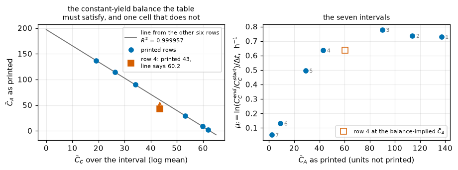
Data: Levenspiel (1999) Problem 29.18 p. 644, attributed by him to
Monod (1958) p. 74. Neither Monod publication was consulted.Four pieces, in increasing order of how much pymrm does:
NumJac((1, 2)) + newton on the two fields \((S, X)\), used as the second, independent computation of route B’s fit: different discretisation, different Jacobian, different linear algebra, and it integrates \(S\) as an unknown rather than substituting the yield relation - so the yield line is tested rather than assumed, through \(S + X/\varphi = {\rm const}\).construct_convflux_upwind + construct_div (nu=0, Cartesian) assemble \(v\,\partial c/\partial z\) once; NumJac((n, 2)) couples the two fields pointwise, which is what a growth law is; newton solves. The chemostat is Rawlings’ eq. (10.18) with the same source term.Boundary conditions use the outward normal. At the inlet \(z=0\) the outward normal points in \(-z\), so the feed is {"a": 0, "b": 1, "d": (S_f, X_f)}; at the outlet it points in \(+z\), so pure outflow is {"a": 1, "b": 0, "d": 0}. Outlet values come from compute_boundary_values, not off the last cell centre; the break table prices reading them there.
# ---------------------------------------------------- the five printed laws
# mu = mu_m * g(theta; S, X).  theta is what is NOT linear.
G = {
 "Monod":    lambda th, S, X: S/(th[0] + S),
 "Blackman": lambda th, S, X: np.minimum(1.0, S/(2*th[0])),
 "Tessier":  lambda th, S, X: 1 - np.exp(-th[0]*S),
 "Moser":    lambda th, S, X: S**th[1]/(th[0] + S**th[1]),
 "Contois":  lambda th, S, X: S/(th[0]*X + S),
 # one-parameter nulls, each best-fitted in its own right
 "zero order":  lambda th, S, X: np.ones_like(S),
 "first order": lambda th, S, X: S/np.max(CAb),
}
NTH  = {"Monod": 1, "Blackman": 1, "Tessier": 1, "Moser": 2, "Contois": 1,
        "zero order": 0, "first order": 0}
LAWS  = ["Monod", "Blackman", "Tessier", "Moser", "Contois"]
NULLS = ["zero order", "first order"]
# GLOBAL scan grids.  A local start is not safe here - see the break table.
RANGE = {"Monod":    np.geomspace(1e-2, 1e5, 240),
         "Blackman": np.geomspace(1e-2, 1e5, 240),
         "Tessier":  np.geomspace(1e-5, 1e1, 240),
         "Contois":  np.geomspace(1e-4, 1e3, 240)}
MOSER_KS, MOSER_N = np.geomspace(1e-2, 1e12, 60), np.linspace(0.3, 6.0, 36)
MUM_LO, MUM_HI = 0.05, 5.0


def thetas(name):
    if NTH[name] == 0:
        return [[]]
    if NTH[name] == 1:
        return [[t] for t in RANGE[name]]
    return [[k, n] for n in MOSER_N for k in MOSER_KS]


def Sof(Cc, a, phi):
    return a - Cc/phi


def profile_mum(gvec, y):
    """route A: mu_m enters linearly, so minimise ||mu_m g - y||^2 in closed form"""
    s = float(np.sum(y*gvec)/np.sum(gvec**2))
    return s, float(np.sum((s*gvec - y)**2))


def fit_A(name, y=mu, X=None):
    X = Xlm if X is None else X
    th = thetas(name)
    sse = np.array([profile_mum(G[name](t, CAb, X), y)[1] for t in th])
    t = list(th[int(np.argmin(sse))])
    if len(t) == 1:                                # refine inside the winning cell
        r = minimize_scalar(lambda v: profile_mum(G[name]([v], CAb, X), y)[1],
                            bounds=(t[0]/1.3, t[0]*1.3), method="bounded",
                            options={"xatol": 1e-13})
        t = [float(r.x)]
    elif len(t) == 2:
        r = minimize(lambda v: profile_mum(G[name]([np.exp(v[0]), v[1]], CAb, X), y)[1],
                     [np.log(t[0]), t[1]], method="Nelder-Mead",
                     options={"xatol": 1e-12, "fatol": 1e-16,
                              "maxiter": 20000, "maxfev": 20000})
        t = [float(np.exp(r.x[0])), float(r.x[1])]
    mum, sse = profile_mum(G[name](t, CAb, X), y)
    pred = mum*G[name](t, CAb, X)
    return dict(p=[mum] + t, sse=sse, rms=float(np.sqrt(sse/len(y))),
                npar=1 + NTH[name], pred=pred, resid=pred - y)


def psi(name, th, a, phi, tau_max=MUM_HI, rtol=1e-8):
    """mu_m-FREE trajectories: dCc/dtau = g(S(Cc)) Cc with tau = mu_m t.
    One dense-output solve per interval prices every mu_m at once."""
    out = []
    for i in range(NOBS):
        rhs = lambda t, y: [G[name](th, max(Sof(y[0], a, phi), 1e-14), y[0])*y[0]]
        out.append(solve_ivp(rhs, [0, tau_max*dt[i]], [Cc0[i]], rtol=rtol,
                             atol=rtol*1e-2, method="LSODA", dense_output=True).sol)
    return out


def mu_pred_ode(name, mum, th, a, phi, rtol=1e-12, method="LSODA"):
    """route B's forward prediction: integrate to the PRINTED dt, adaptively."""
    out = np.empty(NOBS)
    for i in range(NOBS):
        rhs = lambda t, y: [mum*G[name](th, max(Sof(y[0], a, phi), 1e-14), y[0])*y[0]]
        s = solve_ivp(rhs, [0, dt[i]], [Cc0[i]], rtol=rtol, atol=rtol*1e-2,
                      method=method)
        out[i] = np.log(s.y[0, -1]/Cc0[i])/dt[i]
    return out


def fit_B(name, y=mu, a=None, phi=None, p0=None):
    """global scan on route B's OWN objective, then an adaptive-ODE refinement."""
    a = A_BAL if a is None else a
    phi = PHI_BAL if phi is None else phi
    if p0 is None:
        best = (np.inf, None)
        for th in thetas(name):
            sols = psi(name, th, a, phi)
            r = minimize_scalar(
                lambda m: float(np.sum((np.array(
                    [np.log(float(sols[i](m*dt[i])[0])/Cc0[i])/dt[i]
                     for i in range(NOBS)]) - y)**2)),
                bounds=(MUM_LO, MUM_HI), method="bounded", options={"xatol": 1e-7})
            if r.fun < best[0]:
                best = (float(r.fun), [float(r.x)] + list(th))
        p0 = best[1]
    p0 = np.asarray(p0, float)
    lo = [1e-9]*len(p0)
    hi = [50.0] + ([1e12]*NTH[name] if name != "Moser" else [1e12, 10.0])
    r = least_squares(lambda p: mu_pred_ode(name, p[0], p[1:], a, phi) - y, p0,
                      bounds=(lo, hi), xtol=1e-13, ftol=1e-13, gtol=1e-13)
    sse = float(np.sum(r.fun**2))
    return dict(p=list(r.x), sse=sse, rms=float(np.sqrt(sse/len(y))),
                npar=1 + NTH[name], pred=r.fun + y, resid=r.fun)


print("growth laws:", LAWS, "| nulls:", NULLS)
print("global scan:", {k: len(v) for k, v in RANGE.items()},
      "| Moser:", len(MOSER_KS), "x", len(MOSER_N))
growth laws: ['Monod', 'Blackman', 'Tessier', 'Moser', 'Contois'] | nulls: ['zero order', 'first order']
global scan: {'Monod': 240, 'Blackman': 240, 'Tessier': 240, 'Contois': 240} | Moser: 60 x 36class BatchMarch:
"""backward Euler on (S, X) with pymrm's newton + NumJac. Shape (1, 2):
a well-mixed batch is 0-D in space and 2 fields wide, and the growth law is
pointwise in those 2 fields - which is exactly NumJac's default stencil."""
def __init__(self, growth, phi, nstep=200):
self.g, self.phi, self.nstep = growth, phi, nstep
self.shape = (1, 2) # never a bare (2,)
self.numjac = NumJac(self.shape) # last axis coupled in full
def source(self, c):
S = np.clip(c[..., 0:1], 0.0, None)
m = self.g(S, c[..., 1:2])*c[..., 1:2]
return np.concatenate([-m/self.phi, m], axis=-1)
def step(self, c_old, h):
eye = speye(c_old.size, format="csc")
def res(c):
s, js = self.numjac(self.source, c)
return ((c.reshape(-1, 1) - c_old.reshape(-1, 1))/h - s.reshape(-1, 1),
eye/h - js)
out = newton(res, c_old, maxfev=100)
assert out.success, "batch step did not converge"
return out.x.reshape(self.shape)
def march(self, c0, T):
c = np.asarray(c0, float).reshape(self.shape)
h = T/self.nstep
for _ in range(self.nstep):
c = self.step(c, h)
return c
def mu_pred_pymrm(name, mum, th, a, phi, nstep=200):
g = lambda S, X: mum*G[name](th, np.maximum(S, 1e-14), X)
out = np.empty(NOBS)
for i in range(NOBS):
c = BatchMarch(g, phi, nstep).march([[Sof(Cc0[i], a, phi), Cc0[i]]], dt[i])
out[i] = np.log(c[0, 1]/Cc0[i])/dt[i]
return out
class PlugFlowFermenter:
"""Steady 1-D plug flow, fields (S, X), constant yield. pymrm operators."""
def __init__(self, growth, phi, Sf, Xf, tau, ncell=400, v=1.0, nu=0):
self.g, self.phi, self.v, self.tau = growth, phi, v, tau
self.shape = (ncell, 2) # never a bare (ncell,)
self.z_f = np.linspace(0.0, v*tau, ncell + 1)
self.z_c = 0.5*(self.z_f[:-1] + self.z_f[1:])
d0 = np.array([[Sf, Xf]])
# OUTWARD normal, so both dicts read a dc/dn + b c = d.
# z = 0 inlet, outward normal is -z -> Dirichlet feed a=0, b=1, d=(Sf,Xf)
# z = L outlet, outward normal is +z -> pure outflow a=1, b=0, d=0
self.bc = ({"a": 0.0, "b": 1.0, "d": d0},
{"a": 1.0, "b": 0.0, "d": 0.0})
conv, conv_bc = construct_convflux_upwind(self.shape, self.z_f, self.z_c,
self.bc, v=v, axis=0)
self.div = construct_div(self.shape, self.z_f, nu=nu, axis=0) # nu=0 Cartesian
self.A, self.b = self.div @ conv, self.div @ conv_bc
self.numjac = NumJac(self.shape) # pointwise in the 2 fields
self.c0 = np.tile(d0, (ncell, 1))
self.flip = 1.0
def source(self, c):
S = np.clip(c[..., 0:1], 0.0, None)
m = self.g(S, c[..., 1:2])*c[..., 1:2]
return np.concatenate([-self.flip*m/self.phi, m], axis=-1)
def residual(self, c):
s, js = self.numjac(self.source, c)
return (self.b + self.A @ c.reshape((-1, 1)) - s.reshape((-1, 1)),
self.A - js)
def solve(self, strict=True):
r = newton(self.residual, self.c0, maxfev=200)
if strict:
assert r.success, "plug-flow solve did not converge"
self.ok = bool(r.success)
self.c = r.x.reshape(self.shape)
return self
def outlet(self):
"""outlet from compute_boundary_values, NOT the last cell centre"""
return np.asarray(compute_boundary_values(self.c, self.z_f, self.z_c,
self.bc, axis=0)[2]).reshape(-1)[:2]
def batch_reference(growth, phi, S0, X0, tau, rtol=1e-12):
"""the same problem as an initial-value problem - Levenspiel Fig. 29.1"""
rhs = lambda t, y: [-growth(max(y[0], 0.0), y[1])*y[1]/phi,
growth(max(y[0], 0.0), y[1])*y[1]]
s = solve_ivp(rhs, [0, tau], [S0, X0], rtol=rtol, atol=rtol*1e-2, method="LSODA")
return s.y[:, -1]
class Chemostat:
"""Rawlings eq. (10.18), marched to steady state; growth law is a callable."""
def __init__(self, growth, y_yield, Sf, D):
self.g, self.y, self.Sf, self.D = growth, y_yield, Sf, D
def rhs(self, t, c):
S, X = max(c[0], 0.0), c[1]
m = self.g(S, X)
return [self.D*(self.Sf - S) - m*X/self.y, (m - self.D)*X]
def steady(self, tend=40000.0, rtol=1e-11):
s = solve_ivp(self.rhs, [0, tend], [self.Sf, 0.1*self.Sf*self.y],
rtol=rtol, atol=rtol*1e-3, method="LSODA")
return s.y[:, -1]
print("BatchMarch : NumJac((1,2)) + newton, backward Euler on (S, X)")
print("PlugFlowFermenter : construct_convflux_upwind + construct_div(nu=0) + NumJac((n,2)) + newton")
print("Chemostat : Rawlings eq. (10.18), same source term, marched to steady state")BatchMarch : NumJac((1,2)) + newton, backward Euler on (S, X)
PlugFlowFermenter : construct_convflux_upwind + construct_div(nu=0) + NumJac((n,2)) + newton
Chemostat : Rawlings eq. (10.18), same source term, marched to steady stateFit each law’s \(\mu(\bar C_A)\) to the seven \(\mu_i\), with \(\mu_m\) profiled out analytically and the remaining parameter found on a global scan and then refined. Contois needs a biomass too; the exact time average under exponential growth is the logarithmic mean of \(C_C\), which is what is used (the arithmetic mean is a declared convention and a break row).
RA = {k: fit_A(k) for k in LAWS + NULLS}
rows = []
for k in LAWS + NULLS:
    r = RA[k]
    rows.append(dict(law=k, npar=r["npar"], mu_m=r["p"][0],
                     theta=("-" if NTH[k] == 0 else
                            ", ".join(f"{v:.5g}" for v in r["p"][1:])),
                     RMS=r["rms"], SSE=r["sse"]))
TA = pd.DataFrame(rows)
show(TA.style.format({"mu_m": "{:.6f}", "RMS": "{:.6f}", "SSE": "{:.6g}"})
     .hide(axis="index").set_uuid("routeA"))
for k in LAWS + NULLS:
    M[f"rmsA_{k.replace(' ', '_')}"] = RA[k]["rms"]
FA = ((RA["Monod"]["sse"] - RA["Moser"]["sse"])/(RA["Moser"]["sse"]/(NOBS - 3)))
FA_crit = float(f_dist.ppf(0.95, 1, NOBS - 3))
M["routeA_F_moser_vs_monod"] = float(FA)
M["routeA_n_moser"] = float(RA["Moser"]["p"][2])
M["F_crit_95"] = FA_crit
TWO_PAR = ["Monod", "Blackman", "Tessier", "Contois"]
print(f"\nMonod is LAST of the four two-parameter laws on this reduction:"
      f" RMS {RA['Monod']['rms']:.6f} 1/h against Contois {RA['Contois']['rms']:.6f},"
      f"\nTessier {RA['Tessier']['rms']:.6f} and Blackman {RA['Blackman']['rms']:.6f}"
      f" - a factor {RA['Monod']['rms']/RA['Blackman']['rms']:.2f} between the ends.")
print(f"Moser's exponent comes out n = {RA['Moser']['p'][2]:.4f}, and adding it to"
      f" Monod gives\nF = {FA:.4f} against F(1,{NOBS-3}) = {FA_crit:.4f} at 95 % -"
      f" SIGNIFICANT on this reduction.")

# ---- but that significance verdict is CO-CAUSED by the one flagged cell, and
#      this is where a reader meets the claim, so it is priced HERE and not only
#      in meta.yaml.  The imputed value is a labelled INFERENCE, not a repair.
worstA = max(TWO_PAR, key=lambda k: RA[k]["rms"])
CAB_IMPUTED = A_BAL + B_BAL*Xlm[BAD_ROW]
_saveCAb0 = CAb.copy()
try:
    CAb = _saveCAb0.copy()
    CAb[BAD_ROW] = CAB_IMPUTED
    RA_IMP = {k: fit_A(k) for k in LAWS}
finally:
    CAb = _saveCAb0
FA_IMP = float((RA_IMP["Monod"]["sse"] - RA_IMP["Moser"]["sse"])
               / (RA_IMP["Moser"]["sse"]/(NOBS - 3)))
worstA_imp = max(TWO_PAR, key=lambda k: RA_IMP[k]["rms"])
print(f"\nIT IS NOT THE REDUCTION ALONE THAT CLEARS THAT TEST. Put row"
      f" {BAD_ROW+1}'s CA_bar at the\nvalue its own material balance implies,"
      f" {CAB_IMPUTED:.2f} instead of the printed {CAb[BAD_ROW]:.0f} - an"
      f"\nINFERENCE, not a repair, and nothing in the CSV is edited - and route A"
      f" gives\nF = {FA_IMP:.4f} against the same {FA_crit:.4f}: NOT significant."
      f" One printed cell,\nwhich the page flags as off the table's own balance"
      f" line, carries that verdict\nover the threshold on its own.")
print(f"The RANKING claim is unaffected: Blackman still beats Monod with the cell"
      f"\nimputed ({RA_IMP['Blackman']['rms']:.6f} against"
      f" {RA_IMP['Monod']['rms']:.6f}, a factor"
      f" {RA_IMP['Monod']['rms']/RA_IMP['Blackman']['rms']:.2f}\nwhere the printed"
      f" cell gives {RA['Monod']['rms']/RA['Blackman']['rms']:.2f}), and the"
      f" route-A-to-route-B reversal below is the\nreduction. What does move is"
      f" which law comes last of the four: {worstA} on the\nprinted cell,"
      f" {worstA_imp} on the imputed one, and they differ by"
      f" {abs(RA_IMP['Contois']['rms']-RA_IMP['Monod']['rms'])/RA_IMP['Monod']['rms']*100:.2f} %.")

print(f"\nEvery law beats both one-parameter nulls: zero order"
      f" {RA['zero order']['rms']:.6f}, first order\n{RA['first order']['rms']:.6f}"
      f" - Monod is {RA['first order']['rms']/RA['Monod']['rms']:.2f}x better than the"
f" best of them, and Blackman {RA['first order']['rms']/RA['Blackman']['rms']:.2f}x.")| law | npar | mu_m | theta | RMS | SSE |
|---|---|---|---|---|---|
| Monod | 2 | 0.952745 | 28.553 | 0.054690 | 0.0209372 |
| Blackman | 2 | 0.749456 | 24.109 | 0.026772 | 0.0050173 |
| Tessier | 2 | 0.771052 | 0.035009 | 0.038710 | 0.0104891 |
| Moser | 3 | 0.778787 | 346.4, 1.9317 | 0.027117 | 0.0051475 |
| Contois | 2 | 0.833236 | 0.41283 | 0.051534 | 0.01859 |
| zero order | 1 | 0.509681 | - | 0.278278 | 0.542072 |
| first order | 1 | 0.956008 | - | 0.201476 | 0.284149 |
Monod is LAST of the four two-parameter laws on this reduction: RMS 0.054690 1/h against Contois 0.051534,
Tessier 0.038710 and Blackman 0.026772 - a factor 2.04 between the ends.
Moser's exponent comes out n = 1.9317, and adding it to Monod gives
F = 12.2698 against F(1,4) = 7.7086 at 95 % - SIGNIFICANT on this reduction.

IT IS NOT THE REDUCTION ALONE THAT CLEARS THAT TEST. Put row 4's CA_bar at the
value its own material balance implies, 60.18 instead of the printed 43 - an
INFERENCE, not a repair, and nothing in the CSV is edited - and route A gives
F = 5.4477 against the same 7.7086: NOT significant. One printed cell,
which the page flags as off the table's own balance line, carries that verdict
over the threshold on its own.
The RANKING claim is unaffected: Blackman still beats Monod with the cell
imputed (0.040646 against 0.046870, a factor 1.15
where the printed cell gives 2.04), and the route-A-to-route-B reversal below is the
reduction. What does move is which law comes last of the four: Monod on the
printed cell, Contois on the imputed one, and they differ by 0.14 %.

Every law beats both one-parameter nulls: zero order 0.278278, first order
0.201476 - Monod is 3.68x better than the best of them, and Blackman 7.53x.\(\mu_i\) is exactly the interval average of \(\mu\), so the honest comparison integrates the law across the interval instead of evaluating it at \(\bar C_A\). Constant yield makes that a single ODE, and the two constants it needs - \(\varphi\) and \(a\) - come from the material-balance line, which is a property of the printed table and of no growth law. No parameter is added and the models are the same five.
What each route reads, exactly. Both fit the same seven \(\mu_i\), which are the whole of the kinetic information in the table. They differ in where the substrate comes from: route A reads all seven printed \(\bar C_A\) directly, while route B never touches that column at all - it takes the substrate trajectory from \(\varphi\) and \(a\), and those come from the six-row balance line, the one that excludes the flagged row 4. So the datum route A’s ranking leans on hardest is exactly the one route B’s balance line leaves out. That is a real difference between the routes and not a nuisance: the break table prices it directly, refitting every route-B law - and route B’s own \(F\) - with the all-seven balance line instead.
# NO WALL-CLOCK TIMING IS PRINTED ANYWHERE ON THIS PAGE: elapsed seconds differ
# between two consecutive executions, and a page whose stream output is not
# reproducible cannot be diffed, which is how a real drift would be spotted.  The runtime lives in meta.yaml, where it belongs.
RB = {k: fit_B(k) for k in LAWS + NULLS}
rows = []
for k in LAWS + NULLS:
    r = RB[k]
    rows.append(dict(law=k, npar=r["npar"], mu_m=r["p"][0],
                     theta=("-" if NTH[k] == 0 else
                            ", ".join(f"{v:.5g}" for v in r["p"][1:])),
                     RMS=r["rms"], **{"RMS route A": RA[k]["rms"]},
                     **{"B / A": r["rms"]/RA[k]["rms"]}))
TB = pd.DataFrame(rows)
show(TB.style.format({"mu_m": "{:.6f}", "RMS": "{:.6f}", "RMS route A": "{:.6f}",
                      "B / A": "{:.4f}"}).hide(axis="index").set_uuid("routeB"))
for k in LAWS + NULLS:
    M[f"rmsB_{k.replace(' ', '_')}"] = RB[k]["rms"]
FB = ((RB["Monod"]["sse"] - RB["Moser"]["sse"])/(RB["Moser"]["sse"]/(NOBS - 3)))
M["routeB_F_moser_vs_monod"] = float(FB)
M["routeB_n_moser"] = float(RB["Moser"]["p"][2])
M["routeB_monod_mu_m"] = float(RB["Monod"]["p"][0])
M["routeB_monod_K_S"] = float(RB["Monod"]["p"][1])
M["routeA_over_routeB_monod_rms"] = RA["Monod"]["rms"]/RB["Monod"]["rms"]
worstA = max(TWO_PAR, key=lambda k: RA[k]["rms"])
worstB = max(TWO_PAR, key=lambda k: RB[k]["rms"])
print(f"\nThe ranking changes. Monod's residual falls"
      f" {100*(1 - RB['Monod']['rms']/RA['Monod']['rms']):.0f} %, from"
      f" {RA['Monod']['rms']:.6f} to {RB['Monod']['rms']:.6f} 1/h;"
      f"\nthe worst of the four two-parameter laws goes from {worstA} to {worstB}.")
print(f"Moser's exponent drops from {RA['Moser']['p'][2]:.4f} to"
      f" {RB['Moser']['p'][2]:.4f} and F from {FA:.4f} to {FB:.4f}, against the"
      f"\nsame F(1,{NOBS-3}) = {FA_crit:.4f}: NOT significant.")
print(f"\nMonod, route B, FITTED HERE: mu_m = {RB['Monod']['p'][0]:.6f} 1/h,"
      f" K_S = {RB['Monod']['p'][1]:.5f}\nin the units of the printed CA_bar column,"
f" which the source does not print.")| law | npar | mu_m | theta | RMS | RMS route A | B / A |
|---|---|---|---|---|---|---|
| Monod | 2 | 0.880923 | 20.454 | 0.031466 | 0.054690 | 0.5753 |
| Blackman | 2 | 0.721499 | 19.008 | 0.039554 | 0.026772 | 1.4774 |
| Tessier | 2 | 0.756013 | 0.037573 | 0.026308 | 0.038710 | 0.6796 |
| Moser | 3 | 0.793331 | 84.785, 1.5099 | 0.026985 | 0.027117 | 0.9951 |
| Contois | 2 | 0.798109 | 0.29614 | 0.031466 | 0.051534 | 0.6106 |
| zero order | 1 | 0.509681 | - | 0.278278 | 0.278278 | 1.0000 |
| first order | 1 | 0.960801 | - | 0.151597 | 0.201476 | 0.7524 |
The ranking changes. Monod's residual falls 42 %, from 0.054690 to 0.031466 1/h;
the worst of the four two-parameter laws goes from Monod to Blackman.
Moser's exponent drops from 1.9317 to 1.5099 and F from 12.2698 to 1.4389, against the
same F(1,4) = 7.7086: NOT significant.

Monod, route B, FITTED HERE: mu_m = 0.880923 1/h, K_S = 20.45353
in the units of the printed CA_bar column, which the source does not print.
# ---- Contois lands on the Monod curve, to the optimiser's own tolerance
mumC, KsxC = RB["Contois"]["p"]
beta = 1 - KsxC*PHI_BAL
map_mum, map_Ks = mumC/beta, KsxC*PHI_BAL*A_BAL/beta
# THE RULE, stated once here and applied over the WHOLE class in the claims
# cell: a quantity this page PROVES is exactly zero is an optimiser or
# root-finder exit tolerance, not a measurement, so its digits differ between
# machines. It is registered as a BOUND (docs/claims-design.md), checked on
# every run against a limit that holds on any machine, and never compared as a
# value. The printed digits below are this run's; the prose quotes the bound.
MAP_BOUND = 1e-3 # relative: the bound on the two map errors and on S_f/a - 1
RMS_GAP_BOUND = 1e-10 # 1/h: the bound on the Contois-minus-Monod RMS gap
MAP_MUM_RELERR = M["contois_map_mum_relerr"] = float(
abs(map_mum - RB["Monod"]["p"][0])/RB["Monod"]["p"][0])
MAP_KS_RELERR = M["contois_map_KS_relerr"] = float(
abs(map_Ks - RB["Monod"]["p"][1])/RB["Monod"]["p"][1])
CONTOIS_MINUS_MONOD_RMS = M["contois_minus_monod_rms"] = float(
abs(RB["Contois"]["rms"] - RB["Monod"]["rms"]))
print("The Contois fit, pushed through the identity proved in *The published model*:")
print(f" mu_m -> {map_mum:.9f} against the Monod fit's"
f" {RB['Monod']['p'][0]:.9f} (rel. below {MAP_BOUND:g}, here {MAP_MUM_RELERR:.1e})")
print(f" K_S -> {map_Ks:.9f} against the Monod fit's"
f" {RB['Monod']['p'][1]:.9f} (rel. below {MAP_BOUND:g}, here {MAP_KS_RELERR:.1e})")
print(f" residual RMS differs by less than {RMS_GAP_BOUND:g} 1/h (here"
f" {CONTOIS_MINUS_MONOD_RMS:.1e})")
print(" All three of those numbers are BOUNDS, not values: the page proves this")
print(" is one curve fitted twice, so they are two optimisers' exit tolerances,")
print(" and each is checked against a limit that holds on any machine.")
print("\nTwo optimisers, started from different places on two different")
print("parameterisations, landed on the same curve - because it IS the same curve.")The Contois fit, pushed through the identity proved in *The published model*:
mu_m -> 0.880920642 against the Monod fit's 0.880922570 (rel. below 0.001, here 2.2e-06)
K_S -> 20.453271913 against the Monod fit's 20.453534619 (rel. below 0.001, here 1.3e-05)
residual RMS differs by less than 1e-10 1/h (here 4.2e-12)
All three of those numbers are BOUNDS, not values: the page proves this
is one curve fitted twice, so they are two optimisers' exit tolerances,
and each is checked against a limit that holds on any machine.
Two optimisers, started from different places on two different
parameterisations, landed on the same curve - because it IS the same curve.\(\mu\) is curved, so evaluating it at \(\bar C_A\) is not the same as averaging it across the interval. The gap is second order in the substrate swing - and the swing is not small: the last two intervals consume more substrate than their own printed average.
pA = RA["Monod"]["p"]
point_est = pA[0]*G["Monod"](pA[1:], CAb, Xlm)
exact_est = mu_pred_ode("Monod", pA[0], pA[1:], A_BAL, PHI_BAL)
bias = point_est - exact_est
swing = (Cc1 - Cc0)/PHI_BAL                       # substrate consumed in the interval
TBias = pd.DataFrame({"interval": np.arange(1, NOBS+1), "CA_bar printed": CAb,
                      "substrate consumed": swing, "swing / CA_bar": swing/CAb,
                      "mu(CA_bar)": point_est, "<mu> exact": exact_est, "bias": bias})
show(TBias.style.format({"CA_bar printed": "{:.0f}", "substrate consumed": "{:.2f}",
                         "swing / CA_bar": "{:.3f}", "mu(CA_bar)": "{:.5f}",
                         "<mu> exact": "{:.5f}", "bias": "{:+.5f}"})
     .hide(axis="index").set_uuid("bias"))
i_worst = int(np.argmax(np.abs(np.where(np.arange(NOBS) != BAD_ROW, bias, 0.0))))
M["bias_max_abs"] = float(np.max(np.abs(bias)))
M["bias_max_abs_excl_bad_row"] = float(np.abs(bias[i_worst]))
M["bias_over_routeA_rms"] = M["bias_max_abs_excl_bad_row"]/RA["Monod"]["rms"]
M["max_swing_over_CAbar"] = float(np.max(swing/CAb))
print(f"\nLargest bias away from the flagged row: {bias[i_worst]:+.6f} 1/h at"
      f" CA_bar = {CAb[i_worst]:.0f} (interval {i_worst+1}),"
      f"\nwhich is {M['bias_over_routeA_rms']:.2f} times the residual scatter route A"
      f" ranks the five laws on.")
print(f"Row {BAD_ROW+1}'s entry, {bias[BAD_ROW]:+.6f}, is a different animal: it is"
      f" dominated by that row's\ndeparture from the material balance, not by curvature,"
      f" and is reported separately.")
print(f"Largest substrate swing relative to the printed average:"
      f" {M['max_swing_over_CAbar']:.3f} (interval {int(np.argmax(swing/CAb))+1}).")
print("\nThe bias has a SIGN: mu is concave, so mu(mean) exceeds the mean of mu, and")
print("the shortcut therefore makes every saturating law look too gradual near")
print("exhaustion - which is exactly the direction that inflates Moser's exponent.")| interval | CA_bar printed | substrate consumed | swing / CA_bar | mu(CA_bar) | bias | |
|---|---|---|---|---|---|---|
| 1 | 137 | 23.63 | 0.172 | 0.78842 | 0.78728 | +0.00114 |
| 2 | 114 | 22.05 | 0.193 | 0.76191 | 0.76108 | +0.00083 |
| 3 | 90 | 27.72 | 0.308 | 0.72328 | 0.72286 | +0.00042 |
| 4 | 43 | 30.56 | 0.711 | 0.57255 | 0.64111 | -0.06856 |
| 5 | 29 | 30.87 | 1.065 | 0.48007 | 0.46948 | +0.01059 |
| 6 | 9 | 9.45 | 1.050 | 0.22833 | 0.16202 | +0.06631 |
| 7 | 2 | 3.78 | 1.890 | 0.06237 | 0.04997 | +0.01239 |
Largest bias away from the flagged row: +0.066310 1/h at CA_bar = 9 (interval 6),
which is 1.21 times the residual scatter route A ranks the five laws on.
Row 4's entry, -0.068561, is a different animal: it is dominated by that row's
departure from the material balance, not by curvature, and is reported separately.
Largest substrate swing relative to the printed average: 1.890 (interval 7).

The bias has a SIGN: mu is concave, so mu(mean) exceeds the mean of mu, and
the shortcut therefore makes every saturating law look too gradual near
exhaustion - which is exactly the direction that inflates Moser's exponent.Generate data from a Monod model, add Gaussian noise at the observed residual scale, and run route A’s F test on it. Do it twice, changing only what “a Monod model” means:
The second is the control. If route A’s size is inflated in both, the culprit is the small-sample F approximation; if only in the first, it is the reduction.
Every draw is fitted the way route A fits the real data - global scan, then refined. This is not a detail. The observed \(F\) the draws are compared against comes from a refined fit, and reading the draws’ fits off the scan grid with no refinement is worth a factor two in the control’s size: an unrefined Moser fit cannot reach its own optimum, so it under-states \(F\) on every draw and makes the test look conservative when it is not. The refinement is a per-draw zoom on the winning grid cell, its convergence is printed below, and the grid-only numbers are kept as a break row because that is exactly the class of defect - a grid-limited extremum - that no perturbation test can see.
def gmat(name, X=None):
    X = Xlm if X is None else X
    th = thetas(name)
    return np.array([G[name](t, CAb, X) for t in th]), th


GA_M, _ = gmat("Monod")
GA_S, thA_S = gmat("Moser")
nlist = np.array([t[1] for t in thA_S])
DLOG_M = np.log(RANGE["Monod"][1]/RANGE["Monod"][0])     # grid node spacings
DLOG_S, DN_S = np.log(MOSER_KS[1]/MOSER_KS[0]), MOSER_N[1] - MOSER_N[0]
ZOOM = 8                                # refinement rounds; convergence printed


def _sse_M(Y, K):
    """profiled SSE of Monod at a per-draw K (broadcasting over the leading axes)"""
    g = CAb/(K[..., None] + CAb)
    return (np.einsum("...i,...i->...", Y, Y)
            - np.einsum("...i,...i->...", Y, g)**2/np.einsum("...i,...i->...", g, g))


def _sse_S(Y, K, n):
    """profiled SSE of Moser at a per-draw (K, n)"""
    u = CAb**n[..., None]
    g = u/(K[..., None] + u)
    return (np.einsum("...i,...i->...", Y, Y)
            - np.einsum("...i,...i->...", Y, g)**2/np.einsum("...i,...i->...", g, g))


def _zoom1(Y, lk, half, rounds, m=9):
    """per-draw zoom on log K: m nodes across the bracket, halve, repeat"""
    for _ in range(rounds):
        cand = lk[:, None] + np.linspace(-1, 1, m)[None, :]*half[:, None]
        j = np.argmin(_sse_M(Y[:, None, :], np.exp(cand)), axis=1)
        lk, half = cand[np.arange(len(Y)), j], half*2.0/(m - 1)
    return np.exp(lk)


def _zoom2(Y, lk, n, hK, hN, rounds, m=7):
    """the same in two dimensions, on (log K_s, n)"""
    for _ in range(rounds):
        cK = lk[:, None] + np.linspace(-1, 1, m)[None, :]*hK[:, None]
        cN = np.maximum(n[:, None] + np.linspace(-1, 1, m)[None, :]*hN[:, None], 1e-6)
        s = _sse_S(Y[:, None, None, :], np.exp(cK)[:, :, None] + 0*cN[:, None, :],
                   cN[:, None, :] + 0*cK[:, :, None])
        jk, jn = np.unravel_index(np.argmin(s.reshape(len(Y), -1), axis=1), (m, m))
        lk, n = cK[np.arange(len(Y)), jk], cN[np.arange(len(Y)), jn]
        hK, hN = hK*2.0/(m - 1), hN*2.0/(m - 1)
    return np.exp(lk), n


def boot_stats(Y, rounds=None):
    """route-A F statistic and n_hat for a whole block of synthetic datasets.
    Global scan on the SAME grids route A uses, then the SAME refinement:
    rounds=0 reproduces a grid-only fit and is kept as a break row.  Also returns
    a diagnostic dict whose `nclip` is the refinement's convergence evidence,
    counted FROM THE GRID START ALONE - the note under the depth table says why
    it cannot be counted from the shipped pair of starts."""
    rounds = ZOOM if rounds is None else rounds
    nd = len(Y)
    y2 = (Y**2).sum(1)[:, None]
    q1 = y2 - (Y @ GA_M.T)**2/np.einsum("mi,mi->m", GA_M, GA_M)[None, :]
    q2 = y2 - (Y @ GA_S.T)**2/np.einsum("mi,mi->m", GA_S, GA_S)[None, :]
    i1, i2 = np.argmin(q1, axis=1), np.argmin(q2, axis=1)
    if rounds == 0:
        s1, s2 = q1[np.arange(nd), i1], q2[np.arange(nd), i2]
        # nclip is measured from this row's own grid minima; nclip_pair is a
        # STRUCTURAL 0 - there is no pair of starts at depth 0 - and the sum that
        # reports it below excludes this row for exactly that reason.
        return ((s1 - s2)/(s2/(NOBS - 3)), nlist[i2],
                dict(nclip=int(np.sum(s2 > s1*(1 + 1e-12))), nclip_pair=0,
                     ident=0.0, nest_wins=0, best_gain=0.0, flips=0))
    K1 = _zoom1(Y, np.log(RANGE["Monod"][i1]), np.full(nd, DLOG_M), rounds)
    s1 = _sse_M(Y, K1)
    # TWO starts for the two-dimensional fit: the grid winner, and the NESTING
    # POINT n = 1 at the refined Monod K_S.  The second start is a MONOTONICITY
    # GUARANTEE, not a basin escape: at it the Moser objective IS the Monod
    # objective - the same quantity to the last bit, `ident` below - and _zoom2's
    # candidate set contains its own centre, so a fit started there can never end
    # above the Monod fit it is being tested against.  Measured below: it changes
    # no rejection decision on either arm and its largest SSE gain is a few parts
    # in 1e5.  What it buys is that the projection onto the nesting constraint
    # two blocks down is inert - and that is also why the count of draws where
    # that projection binds measures nothing at all.
    ident = float(np.max(np.abs(_sse_S(Y, K1, np.ones(nd)) - s1)))
    sols = []
    for lk0, n0 in ((np.log(np.array([thA_S[j][0] for j in i2])),
                     np.array([thA_S[j][1] for j in i2])),
                    (np.log(K1), np.ones(nd))):
        K2, n2 = _zoom2(Y, lk0, n0, np.full(nd, DLOG_S), np.full(nd, DN_S), rounds)
        sols.append((_sse_S(Y, K2, n2), n2))
    take = sols[0][0] <= sols[1][0]
    s2 = np.where(take, sols[0][0], sols[1][0])
    nhat = np.where(take, sols[0][1], sols[1][1])
    # Moser CONTAINS Monod, so its SSE cannot exceed Monod's, and a fit that ends
    # above it is not converged.  That count is informative for the GRID START
    # (nclip) and is identically zero for the shipped pair (nclip_pair), for the
    # reason given above; both are returned and both are printed.
    nclip = int(np.sum(sols[0][0] > s1*(1 + 1e-12)))
    nclip_pair = int(np.sum(s2 > s1*(1 + 1e-12)))
    gain = float(np.max((sols[0][0] - s2)/s2))
    sg = np.minimum(sols[0][0], s1)                 # the grid start on its own
    F_grid = (s1 - sg)/(sg/(NOBS - 3))
    s2 = np.minimum(s2, s1)
    F = (s1 - s2)/(s2/(NOBS - 3))
    return F, nhat, dict(nclip=nclip, nclip_pair=nclip_pair, ident=ident,
                         nest_wins=int(np.sum(sols[1][0] < sols[0][0])),
                         best_gain=gain,
                         flips=int(np.sum((F > FA_crit) != (F_grid > FA_crit))))


def prop_se(p):
    """binomial standard error of a bootstrap frequency, at NBOOT draws"""
    return float(np.sqrt(p*(1.0 - p)/NBOOT))


def median_se(v):
    """distribution-free standard error of a median, from the order statistics:
    half the width of the interval the binomial sign count puts one standard
    deviation either side of the middle rank.  No RNG, so it is deterministic."""
    w, N = np.sort(v), len(v)
    k = 0.5*np.sqrt(N)
    return float(0.5*(w[min(N - 1, int(np.ceil(N/2 + k)))]
                      - w[max(0, int(np.floor(N/2 - k)))]))


def boot_arm(yt, sd, seed=None, rounds=None):
    Y = yt[None, :] + np.random.default_rng(SEED if seed is None else seed
                                            ).normal(0.0, sd, (NBOOT, NOBS))
    Fb, nb, dg = boot_stats(Y, rounds)
    size = float((Fb > FA_crit).mean())
    pF, pn = float((Fb > FA).mean()), float((nb > RA["Moser"]["p"][2]).mean())
    # EVERY number below is a Monte-Carlo estimate at NBOOT draws - `size`, `pF`
    # and `pn` are frequencies, `med` is a median - so every one of them carries
    # a sampling error, printed beside it everywhere it is quoted: prop_se is the
    # binomial one and median_se the order-statistic one
    return dict(size=size, med=float(np.median(nb)), pF=pF, pn=pn,
                size_se=prop_se(size), pF_se=prop_se(pF), pn_se=prop_se(pn),
                med_se=median_se(nb), **dg)


sigma, NBOOT = RB["Monod"]["rms"], 2000
y_true = mu_pred_ode("Monod", RB["Monod"]["p"][0], RB["Monod"]["p"][1:],
                     A_BAL, PHI_BAL)
y_ctrl = point_est                                  # route A's own model
ARMS = (("forward", y_true), ("control", y_ctrl))

# ---- refinement evidence FIRST: the six numbers against the zoom depth
print(f"{NBOOT} seeded draws each, sigma = {sigma:.6f} 1/h, seed {SEED},"
      f" nominal size 0.0500")
print("\nrefinement of each draw's fit (rounds = 0 is the grid alone; the grid is"
      f"\n{len(RANGE['Monod'])} Monod nodes and {len(MOSER_KS)} x {len(MOSER_N)}"
      f" Moser nodes, an n spacing of {DN_S:.3f}):\n")
print(f"{'rounds':>7}{'fwd size':>10}{'fwd med n':>11}{'fwd p':>8}"
      f"{'ctrl size':>11}{'ctrl med n':>12}{'unconverged':>13}")
CONV = {}
for r in (0, 2, 4, 6, ZOOM):
    CONV[r] = {tag: boot_arm(yt, sigma, rounds=r) for tag, yt in ARMS}
    f_, c_ = CONV[r]["forward"], CONV[r]["control"]
    print(f"{r:>7}{f_['size']:>10.4f}{f_['med']:>11.4f}{f_['pF']:>8.4f}"
          f"{c_['size']:>11.4f}{c_['med']:>12.4f}"
          f"{f_['nclip'] + c_['nclip']:>13d}"
          + ("   <- the grid alone" if r == 0 else
             "   <- converged, used below" if r == ZOOM else ""))
# summed over the REFINED rows only: the rounds = 0 row is fitted from the grid
# winner alone, so it has no pair of starts and its entry is a structural 0 the
# code writes rather than a count it takes - folding that in would have made the
# claim below rest partly on a hard-coded zero.
N_REFINED = sum(1 for r in CONV if r > 0)
N_PAIR_CLIP = sum(CONV[r][t]["nclip_pair"]
                  for r in CONV if r > 0 for t in ("forward", "control"))
IDENT_MAX = max(CONV[r][t]["ident"] for r in CONV for t in ("forward", "control"))
print(f"\n  'unconverged' counts the draws, out of {2*NBOOT}, on which the"
      f" two-dimensional fit\n  STARTED FROM THE GRID WINNER ALONE still ends ABOVE"
      f" the one-dimensional one -\n  impossible for a converged fit, since Moser"
      f" contains Monod. Read it as the\n  convergence evidence for the zoom, and"
      f" read the six numbers' own trend beside\n  it: both say the same thing about"
      f" where this table settles.")
print(f"\n  WHAT IT CANNOT SHOW. The same count for the fit actually shipped - the"
      f" pair of\n  starts - is {N_PAIR_CLIP} summed over the {N_REFINED} REFINED rows"
      f" above (the grid-only row is\n  fitted from the grid winner alone, so it has no"
      f" pair of starts and no such\n  count), and it cannot be anything else at any"
      f" refined depth: the second start IS\n  the nesting point, where the Moser"
      f" objective and the Monod objective are the\n  same number to the last bit"
      f" (largest difference over all {2*NBOOT} draws and all\n  depths:"
      f" {IDENT_MAX:.1e}), and the zoom's candidate set contains its"
      f"\n  own centre, so that branch is monotone and can never end above it. A"
      f" column of\n  zeros there would be an identity of the code, not a"
      f" measurement, so it is not\n  what is printed. The shipped fit is at least"
      f" as converged as the column says.")
out = CONV[ZOOM]
GRID_ONLY = CONV[0]
M["boot_size_forward_truth"] = out["forward"]["size"]
M["boot_size_control_truth"] = out["control"]["size"]
M["boot_median_n_forward_truth"] = out["forward"]["med"]
M["boot_median_n_control_truth"] = out["control"]["med"]
M["boot_p_of_observed_F"] = out["forward"]["pF"]
M["boot_p_of_observed_n"] = out["forward"]["pn"]

pm = lambda v, s: f"{v:.4f} +- {s:.4f}"
print(f"\n{'truth':<46}{'size':>18}{'median n':>18}{'p(F>obs)':>18}")
for tag, lab in (("forward", "the forward Monod model (what Monod produces)"),
                 ("control", "mu(CA_bar) - route A's own model [CONTROL]")):
    o = out[tag]
    print(f"{lab:<46}{pm(o['size'], o['size_se']):>18}"
          f"{pm(o['med'], o['med_se']):>18}{pm(o['pF'], o['pF_se']):>18}")
print(f"\nand on the forward arm, p for the OBSERVED exponent:"
      f" {pm(out['forward']['pn'], out['forward']['pn_se'])}")
print(f"\nEVERY NUMBER IN THAT TABLE AND IN THE LINE UNDER IT IS A MONTE-CARLO"
      f" ESTIMATE over\n{NBOOT} seeded draws, and they are NOT all of one kind: the"
      f" sizes and the p values\nare FREQUENCIES, the two exponents are MEDIANS. So"
      f" every one carries a sampling\nerror, printed beside it as +- one standard"
      f" error - binomial for the frequencies,\nand from the order statistics for the"
      f" medians.")


def sig_stable(v, s):
    """how many leading significant figures of v its own standard error s
    supports: the largest k with s below half a unit in the k-th figure."""
    k = 0
    while s < 0.5*10.0**(int(np.floor(np.log10(abs(v)))) - k) and k < 6:
        k += 1
    return k


SIX = [("forward size", out["forward"]["size"], out["forward"]["size_se"]),
       ("control size", out["control"]["size"], out["control"]["size_se"]),
       ("p(F>obs)", out["forward"]["pF"], out["forward"]["pF_se"]),
       ("p(n>obs)", out["forward"]["pn"], out["forward"]["pn_se"]),
       ("forward median n", out["forward"]["med"], out["forward"]["med_se"]),
       ("control median n", out["control"]["med"], out["control"]["med_se"])]
K_FIG = {lab: sig_stable(v, s) for lab, v, s in SIX}
FREQ6 = ("forward size", "control size", "p(F>obs)", "p(n>obs)")
MED6 = ("forward median n", "control median n")
print(f"\nAND HOW MANY FIGURES THAT BUYS, PER STATISTIC rather than in one sentence"
      f" - for\nthe six quoted off this page, the largest k whose k-th significant"
      f" figure one\nstandard error does not reach:\n")
for lab, v, s in SIX:
    half = 0.5*10.0**(int(np.floor(np.log10(abs(v)))) - K_FIG[lab])
    print(f"   {lab:<17}{v:>8.4f} +- {s:<7.4f} one SE is {s/half:>5.1f}x half a unit"
          f" in figure {K_FIG[lab] + 1}"
          f" ({half:.4g}) -> {K_FIG[lab]} figure" + ("s" if K_FIG[lab] != 1 else ""))
# what meta.yaml, README.md and models_entry.yaml say about these six - "the
# frequencies to their leading figure only, the medians to at least two" - is
# this table, and it is ASSERTED here rather than trusted to stay true
assert max(K_FIG[lab] for lab in FREQ6) <= 1, K_FIG
assert min(K_FIG[lab] for lab in MED6) >= 2, K_FIG
print(f"\nSo the FREQUENCIES are seed-independent in their LEADING FIGURE ONLY"
      f" ({max(K_FIG[lab] for lab in FREQ6)} figure), and\nthe MEDIANS in at least"
      f" {min(K_FIG[lab] for lab in MED6)}. The four-figure values above are exact for"
      f" THIS seed and\nreproducible, not resolved - read the +-, not the digit count."
      f" Every quotation of\nthem on this page carries the same +-.")
print(f"\nThe control sits AT its nominal size ({out['control']['size']:.4f} +-"
      f" {out['control']['size_se']:.4f} against 0.0500) and\nrecovers the truth's"
      f" exponent ({out['control']['med']:.4f} +- {out['control']['med_se']:.4f}"
      f" against 1). So the small-sample F\napproximation at n = 7 is essentially EXACT"
      f" here - it is not conservative, and it\nis not the problem. Against data Monod"
      f" actually produces, the same test rejects\nit {out['forward']['size']:.1%} +-"
      f" {out['forward']['size_se']:.1%} of the time and puts the median exponent at"
      f" {out['forward']['med']:.4f} +- {out['forward']['med_se']:.4f}.\nThe whole of"
      f" the distortion is the reduction.")
print(f"\nWHAT THE SECOND START DOES, measured on the converged row rather than"
      f" asserted:\nit strictly wins on"
      f" {out['forward']['nest_wins'] + out['control']['nest_wins']} of the"
      f" {2*NBOOT} draws, but the largest SSE it ever gains is"
      f"\n{max(out['forward']['best_gain'], out['control']['best_gain']):.1e} relative,"
      f" and it changes"
      f" {out['forward']['flips'] + out['control']['flips']} rejection decisions on the"
      f" two arms combined.\nIt is a monotonicity guarantee - the fit can never end"
      f" above the Monod fit it is\nbeing tested against - and not an escape from a"
      f" wrong basin.")
print(f"\nRead the first row of the table above the same way: fitted on the grid"
      f" alone,\nthe control reads {GRID_ONLY['control']['size']:.4f} and its median"
      f" exponent {GRID_ONLY['control']['med']:.4f} - a coarse Moser grid\n(n spacing"
      f" {DN_S:.3f}) cannot reach its own optimum, so it deflates F on every draw and"
      f"\nmanufactures a conservative-looking control. That is a grid-limited"
      f" extremum,\nand no perturbation of the model would have revealed it.")
print(f"\nThe OBSERVED route-A verdict, F = {FA:.4f}, therefore has p ="
      f" {out['forward']['pF']:.4f} +- {out['forward']['pF_se']:.4f}\nagainst a"
      f" properly generated Monod null - not significant at all, and not close"
      f"\nenough to 0.05 for the sampling error to matter - and its exponent"
      f"\nn = {RA['Moser']['p'][2]:.4f} has p ="
      f" {out['forward']['pn']:.4f} +- {out['forward']['pn_se']:.4f}.")

# ---- the noise scale is a DECLARED CONVENTION for the forward arm, and is not
#      one for the control.  Both are printed rather than asserted.
SIG_ALT = {"route B RMS (used above)": sigma, "route A RMS": RA["Monod"]["rms"]}
SIG_TABLE = {lab: (boot_arm(y_true, sd)["size"], boot_arm(y_ctrl, sd)["size"])
             for lab, sd in SIG_ALT.items()}
print(f"\nWhich residual scatter supplies sigma is a declared convention, and it"
      f" matters\nfor one arm only:\n")
print(f"{'sigma':<26}{'value, 1/h':>12}{'forward size':>18}{'control size':>18}")
for lab, sd in SIG_ALT.items():
    print(f"{lab:<26}{sd:>12.6f}{pm(SIG_TABLE[lab][0], prop_se(SIG_TABLE[lab][0])):>18}"
          f"{pm(SIG_TABLE[lab][1], prop_se(SIG_TABLE[lab][1])):>18}")
print(f"\nThe FORWARD size is a bias-to-noise ratio, so it moves with sigma and the"
      f"\nquoted {out['forward']['size']:.1%} +- {out['forward']['size_se']:.1%} is"
      f" specific to route B's scatter. The"
      f" CONTROL's size is scale-free to\nMonte-Carlo error, which is exactly what a"
      f" correctly specified test should do,\nand is a second reason to read it as"
      f" the F approximation being exonerated.")
2000 seeded draws each, sigma = 0.031466 1/h, seed 20260813, nominal size 0.0500
refinement of each draw's fit (rounds = 0 is the grid alone; the grid is
240 Monod nodes and 60 x 36 Moser nodes, an n spacing of 0.163):
rounds fwd size fwd med n fwd p ctrl size ctrl med n unconverged
0 0.3080 1.6029 0.1835 0.0210 0.9514 994 <- the grid alone
2 0.3640 1.6029 0.2265 0.0485 1.0000 131
4 0.3655 1.6119 0.2280 0.0495 1.0097 11
6 0.3655 1.6116 0.2280 0.0495 1.0088 0
8 0.3655 1.6117 0.2280 0.0495 1.0089 0 <- converged, used below
'unconverged' counts the draws, out of 4000, on which the two-dimensional fit
STARTED FROM THE GRID WINNER ALONE still ends ABOVE the one-dimensional one -
impossible for a converged fit, since Moser contains Monod. Read it as the
convergence evidence for the zoom, and read the six numbers' own trend beside
it: both say the same thing about where this table settles.
WHAT IT CANNOT SHOW. The same count for the fit actually shipped - the pair of
starts - is 0 summed over the 4 REFINED rows above (the grid-only row is
fitted from the grid winner alone, so it has no pair of starts and no such
count), and it cannot be anything else at any refined depth: the second start IS
the nesting point, where the Moser objective and the Monod objective are the
same number to the last bit (largest difference over all 4000 draws and all
depths: 0.0e+00), and the zoom's candidate set contains its
own centre, so that branch is monotone and can never end above it. A column of
zeros there would be an identity of the code, not a measurement, so it is not
what is printed. The shipped fit is at least as converged as the column says.
truth size median n p(F>obs)
the forward Monod model (what Monod produces) 0.3655 +- 0.0108 1.6117 +- 0.0074 0.2280 +- 0.0094
mu(CA_bar) - route A's own model [CONTROL] 0.0495 +- 0.0049 1.0089 +- 0.0049 0.0240 +- 0.0034
and on the forward arm, p for the OBSERVED exponent: 0.1285 +- 0.0075
EVERY NUMBER IN THAT TABLE AND IN THE LINE UNDER IT IS A MONTE-CARLO ESTIMATE over
2000 seeded draws, and they are NOT all of one kind: the sizes and the p values
are FREQUENCIES, the two exponents are MEDIANS. So every one carries a sampling
error, printed beside it as +- one standard error - binomial for the frequencies,
and from the order statistics for the medians.
AND HOW MANY FIGURES THAT BUYS, PER STATISTIC rather than in one sentence - for
the six quoted off this page, the largest k whose k-th significant figure one
standard error does not reach:
forward size 0.3655 +- 0.0108 one SE is 2.2x half a unit in figure 2 (0.005) -> 1 figure
control size 0.0495 +- 0.0049 one SE is 9.7x half a unit in figure 2 (0.0005) -> 1 figure
p(F>obs) 0.2280 +- 0.0094 one SE is 1.9x half a unit in figure 2 (0.005) -> 1 figure
p(n>obs) 0.1285 +- 0.0075 one SE is 1.5x half a unit in figure 2 (0.005) -> 1 figure
forward median n 1.6117 +- 0.0074 one SE is 1.5x half a unit in figure 3 (0.005) -> 2 figures
control median n 1.0089 +- 0.0049 one SE is 9.7x half a unit in figure 4 (0.0005) -> 3 figures
So the FREQUENCIES are seed-independent in their LEADING FIGURE ONLY (1 figure), and
the MEDIANS in at least 2. The four-figure values above are exact for THIS seed and
reproducible, not resolved - read the +-, not the digit count. Every quotation of
them on this page carries the same +-.
The control sits AT its nominal size (0.0495 +- 0.0049 against 0.0500) and
recovers the truth's exponent (1.0089 +- 0.0049 against 1). So the small-sample F
approximation at n = 7 is essentially EXACT here - it is not conservative, and it
is not the problem. Against data Monod actually produces, the same test rejects
it 36.5% +- 1.1% of the time and puts the median exponent at 1.6117 +- 0.0074.
The whole of the distortion is the reduction.
WHAT THE SECOND START DOES, measured on the converged row rather than asserted:
it strictly wins on 903 of the 4000 draws, but the largest SSE it ever gains is
9.9e-05 relative, and it changes 0 rejection decisions on the two arms combined.
It is a monotonicity guarantee - the fit can never end above the Monod fit it is
being tested against - and not an escape from a wrong basin.
Read the first row of the table above the same way: fitted on the grid alone,
the control reads 0.0210 and its median exponent 0.9514 - a coarse Moser grid
(n spacing 0.163) cannot reach its own optimum, so it deflates F on every draw and
manufactures a conservative-looking control. That is a grid-limited extremum,
and no perturbation of the model would have revealed it.
The OBSERVED route-A verdict, F = 12.2698, therefore has p = 0.2280 +- 0.0094
against a properly generated Monod null - not significant at all, and not close
enough to 0.05 for the sampling error to matter - and its exponent
n = 1.9317 has p = 0.1285 +- 0.0075.
Which residual scatter supplies sigma is a declared convention, and it matters
for one arm only:
sigma value, 1/h forward size control size
route B RMS (used above) 0.031466 0.3655 +- 0.0108 0.0495 +- 0.0049
route A RMS 0.054690 0.2355 +- 0.0095 0.0470 +- 0.0047
The FORWARD size is a bias-to-noise ratio, so it moves with sigma and the
quoted 36.5% +- 1.1% is specific to route B's scatter. The CONTROL's size is scale-free to
Monte-Carlo error, which is exactly what a correctly specified test should do,
and is a second reason to read it as the F approximation being exonerated.Identifiability is a property of the experiment, not of the model. Take Monod as true, at the route-B fit; ask how close each alternative can get to it at these seven design points; and compare that distance with the scatter. \(N^*\) is the number of independent repeats of the seven-interval run - Levenspiel’s Problem 29.18, attributed by him to Monod (1958) - at which a \(\chi^2\) separation at 95 % becomes possible.
Read \(N^*\) as a threshold, not as a sample size. It is the \(N\) at which the expected excess sum of squares first reaches the 95 % critical value. An experiment run at exactly \(N^*\) therefore lands above the critical value about half the time: \(N^*\) is roughly a 50 %-power point, not a 95 %-detection design. Three further choices in it - the confidence level, the degrees of freedom, and which route supplies the scatter - are declared conventions with break rows, and the separations \(d\) that go into it are optimiser upper bounds, so \(N^*\) errs low in the direction that matters.
s_obs = RB["Monod"]["rms"]
SEP_BOUND = 1e-9          # 1/h: the bound the two degenerate separations are held to
SEP_SCATTER_BOUND = 1e-7  # the same, over the route-B scatter
SEP = {}
sep_rows = []
for k in ["Blackman", "Tessier", "Moser", "Contois"]:
    r = fit_B(k, y=y_true, p0=RB[k]["p"])       # warm start: the manifold is the same
    d = r["rms"]
    SEP[k] = d
    Nstar = (chi2.ppf(0.95, NOBS - 2)*s_obs**2/(NOBS*d**2)) if d > 1e-9 else np.inf
    sep_rows.append(dict(alternative=k, d=d, **{"d / scatter": d/s_obs},
                         **{"N* repeats": Nstar},
                         verdict=("degenerate - see the identities" if d < 1e-9 else
                                  "within reach of one clean run, at ~50 % power"
                                  if Nstar <= 1.5 else "needs more data")))
    # every separation is a claim; the degenerate two are BOUNDS (the rule stated
    # where the Contois map is computed), registered as such in the claims cell
    M[f"sep_{k.lower()}"] = float(d)
    M[f"sep_over_scatter_{k.lower()}"] = float(d/s_obs)
    if np.isfinite(Nstar):     # only where a separation exists at all: for Moser
        M[f"Nstar_{k.lower()}"] = float(Nstar)   # and Contois it is not a number

TS = pd.DataFrame(sep_rows)
show(TS.style.format({"d": "{:.4e}", "d / scatter": "{:.5f}", "N* repeats": "{:.4g}"})
     .hide(axis="index").set_uuid("sep"))
print("\nMoser and Contois sit at the optimiser's own floor, and that is not an")
print("accident of this dataset - it is the algebra of *The published model*: Moser")
print("CONTAINS Monod at n = 1, and Contois IS Monod once a constant yield makes X an")
print("affine function of S. Their symbolic residuals are exactly zero; the numbers")
print(f"above (here {SEP['Moser']:.1e} and {SEP['Contois']:.1e}) measure"
      f" least_squares' xtol, not a\nseparation, so both are registered as BOUNDS,"
      f" below {SEP_BOUND:g} 1/h, and never compared as values.")
print(f"\nTessier and Blackman are genuinely separable. Blackman needs"
      f" {M['Nstar_blackman']:.2f} repeats of this")
print(f"design and Tessier {M['Nstar_tessier']:.1f}. So one clean run of it is"
      f" within {100*(M['Nstar_blackman']-1):.0f} % of enough for")
print(f"Blackman - not enough, and at N* the power is only about a half anyway,")
print(f"so 'one run would do' would be generous twice over.")
print("\nNote which way this cuts against route A: Blackman, the law route A liked")
print("best, is the ONLY one this design can actually resolve - so route A's ranking")
print("is not merely biased, it is confidently ordering laws it cannot tell apart.")| alternative | d | d / scatter | N* repeats | verdict |
|---|---|---|---|---|
| Blackman | 3.4659e-02 | 1.10148 | 1.304 | within reach of one clean run, at ~50 % power |
| Tessier | 1.2348e-02 | 0.39242 | 10.27 | needs more data |
| Moser | 2.4883e-14 | 0.00000 | inf | degenerate - see the identities |
| Contois | 6.3274e-14 | 0.00000 | inf | degenerate - see the identities |
Moser and Contois sit at the optimiser's own floor, and that is not an
accident of this dataset - it is the algebra of *The published model*: Moser
CONTAINS Monod at n = 1, and Contois IS Monod once a constant yield makes X an
affine function of S. Their symbolic residuals are exactly zero; the numbers
above (here 2.5e-14 and 6.3e-14) measure least_squares' xtol, not a
separation, so both are registered as BOUNDS, below 1e-09 1/h, and never compared as values.

Tessier and Blackman are genuinely separable. Blackman needs 1.30 repeats of this
design and Tessier 10.3. So one clean run of it is within 30 % of enough for
Blackman - not enough, and at N* the power is only about a half anyway,
so 'one run would do' would be generous twice over.

Note which way this cuts against route A: Blackman, the law route A liked
best, is the ONLY one this design can actually resolve - so route A's ranking
is not merely biased, it is confidently ordering laws it cannot tell apart.
The degeneracy above is a property of a constant-yield batch run, which ties \(X\) to \(S\). A chemostat does not: the dilution rate moves them independently. Rawlings’ eq. (10.18) with a Monod law washes out at \(D_c = \mu_m S_f/(K_s + S_f)\), which depends on the feed concentration. With a Contois law the same balance gives \(\mu \to \mu_m\) as \(X \to 0\), so \(D_c = \mu_m\) whatever the feed. The two cross - and the crossing point is not arbitrary.
mumM, KsM = RB["Monod"]["p"]
Dc_monod = lambda Sf: mumM*Sf/(KsM + Sf)
Dc_contois = mumC                                     # independent of S_f, exactly
ratio = lambda Sf: Dc_contois/Dc_monod(Sf)
Sf_cross = brentq(lambda Sf: ratio(Sf) - 1.0, 1.0, 1e4, xtol=1e-10, rtol=8.9e-16)
Sf_10pct = brentq(lambda Sf: ratio(Sf) - 1.10, 1.0, 1e4, xtol=1e-10, rtol=8.9e-16)
M["Sf_crossing"] = float(Sf_cross)
M["Sf_for_10pct_gap"] = float(Sf_10pct)
M["Dc_ratio_at_Sf20"] = float(ratio(20.0))
SF_CLOSED = mumC*KsM/(mumM - mumC)        # the same crossing, in closed form
SF_ROOTFIND_RELERR = abs(Sf_cross - SF_CLOSED)/SF_CLOSED
# brentq's OWN guarantee, from the tolerances declared two lines up rather than
# from the residual that happened to come out: scipy returns an x0 with
# |x0 - x*| <= xtol + rtol|x0|, which is 5.1e-13 relative here.  The observed
# residual is three orders inside that, but it is a property of Brent's last
# interpolation, not of anything declared - it moves 40x under a change of
# BRACKET that changes nothing about the mathematics - so the assertion cell
# tests it against this bound and not against the value below.
SF_XTOL, SF_RTOL = 1e-10, 8.9e-16
SF_ROOTFIND_BOUND = (SF_XTOL + SF_RTOL*abs(Sf_cross))/SF_CLOSED
CROSS_VS_A = M["Sf_crossing_vs_a_relerr"] = float(abs(Sf_cross - A_BAL)/A_BAL)
# The two exit tolerances of the Contois fit, SIGNED, and the sensitivity of the
# closed form to each.  S_f/a = (1+e_mu)/[(1+e_K)(1 - e_mu beta/(1-beta))], so to
# first order S_f/a - 1 = e_mu/(1-beta) - e_K: the mu_m error is amplified by
# 1/(1-beta) and the K_S error enters with coefficient EXACTLY 1.
E_MUM = (map_mum - mumM)/mumM
E_KS = (map_Ks - KsM)/KsM
AMP = 1/(1 - beta)
CROSS_DECOMP = E_MUM*AMP - E_KS
print("The crossing is EXACT, and it is the batch run's own substrate intercept:")
print("  putting mu_m^C = beta mu_m^M and K_S = K_sx phi a / beta into")
print("  mu_m^M S_f/(K_S + S_f) = mu_m^C gives S_f = a identically. Numerically:")
print(f"    root-found crossing        S_f = {Sf_cross:.6f}")
print(f"    material-balance intercept a   = {A_BAL:.6f}"
      f"   (rel. gap below {MAP_BOUND:g}, here {CROSS_VS_A:.2e})")
print(f"\n  That gap is NOT the root-find's. Solving the same equation in closed form,"
      f"\n  S_f = mu_m^C K_S/(mu_m^M - mu_m^C) = {SF_CLOSED:.6f}, and brentq reproduces it"
      f" to\n  {SF_ROOTFIND_RELERR:.1e} - at round-off, and inside its own"
      f" declared\n  guarantee (xtol + rtol|x| = {SF_ROOTFIND_BOUND:.1e} relative here),"
      f" which is what is asserted.")
print(f"\n  What the {CROSS_VS_A:.2e} measures is the Contois fit's own two exit"
      f" tolerances, and\n  NOT in equal measure. Differentiating that closed form:"
      f" d ln S_f / d ln mu_m^C =\n  1/(1-beta) = {AMP:.3f}, while d ln S_f / d ln K_S"
      f" = 1 EXACTLY. So it is the mu_m error\n  that is amplified and the K_S error"
      f" that is not:")
print(f"      mu_m error {E_MUM:+.3e}, amplified x {AMP:.3f}    contributes"
      f" {E_MUM*AMP:+.3e}")
print(f"      K_S  error {E_KS:+.3e}, unamplified, other sign  contributes"
      f" {-E_KS:+.3e}")
print(f"                                                        sum"
      f" {CROSS_DECOMP:+.3e}\n      - which is the {CROSS_VS_A:.2e} above.")
# the decomposition is the justification for treating this quantity as a
# tolerance bound, so it is checked rather than left as prose: the first-order
# form is good to 1e-5
assert abs(abs(CROSS_DECOMP) - CROSS_VS_A) <= 5e-3*CROSS_VS_A, (CROSS_DECOMP, CROSS_VS_A)
print(f"\n  The K_S error alone is within"
      f" {100*abs(abs(E_KS)/CROSS_VS_A - 1):.0f} % of the {CROSS_VS_A:.2e}, which is a"
      f" coincidence and\n  not an explanation: amplify THAT one by the {AMP:.1f}"
      f" instead and you get {abs(E_KS)*AMP:.2e},\n  {abs(E_KS)*AMP/CROSS_VS_A:.0f} times the"
      f" number being explained. Either way it is the same exactly-zero\n  quantity as"
      f" the two map errors, and it is a BOUND for the same reason: below"
      f" {MAP_BOUND:g}\n  relative, checked on every run.")
print(f"\n  Away from it they separate: at S_f = 20 the two critical dilution rates"
      f"\n  differ by a factor {M['Dc_ratio_at_Sf20']:.4f}, and the gap exceeds 10 %"
      f" for every S_f\n  below {Sf_10pct:.2f} - in the units of the printed CA_bar"
      f" column, whose scale is set\n  by the run itself (its substrate ran from"
      f" {A_BAL - Cc0[0]/PHI_BAL:.1f} to {A_BAL - Cc1[-1]/PHI_BAL:.2f}).")

Sf_test, y_yield = 20.0, PHI_BAL
gM_ = lambda S, X: mumM*S/(KsM + S)
gC_ = lambda S, X: mumC*S/(KsxC*X + S)
WASH = 1e-6
Dc_num = {}
for tag, g_ in (("Monod", gM_), ("Contois", gC_)):
    Dc_num[tag] = brentq(lambda D: Chemostat(g_, y_yield, Sf_test, D).steady()[1]
                         - WASH*y_yield*Sf_test, 0.05, 2.0, xtol=1e-9, rtol=8.9e-16)
M["Dc_monod_closed_form"] = float(Dc_monod(Sf_test))
M["Dc_monod_transient_relerr"] = abs(Dc_num["Monod"] - Dc_monod(Sf_test))/Dc_monod(Sf_test)
M["Dc_contois_transient_relerr"] = abs(Dc_num["Contois"] - Dc_contois)/Dc_contois
print(f"\n  washout root-found on a MARCHED chemostat, S_f = {Sf_test:.0f}:")
print(f"    Monod   D_c = {Dc_num['Monod']:.8f} against the closed form"
      f" {Dc_monod(Sf_test):.8f}  (rel. {M['Dc_monod_transient_relerr']:.2e})")
print(f"    Contois D_c = {Dc_num['Contois']:.8f} against mu_m ="
      f" {Dc_contois:.8f}  (rel. {M['Dc_contois_transient_relerr']:.2e})")
print(f"\n  Two models that no batch run can tell apart differ by a factor"
      f" {M['Dc_ratio_at_Sf20']:.2f} in the\n  dilution rate at which the culture is"
      f" lost. That is the experiment to run.")
The crossing is EXACT, and it is the batch run's own substrate intercept:
putting mu_m^C = beta mu_m^M and K_S = K_sx phi a / beta into
mu_m^M S_f/(K_S + S_f) = mu_m^C gives S_f = a identically. Numerically:
root-found crossing S_f = 197.118211
material-balance intercept a = 197.120267 (rel. gap below 0.001, here 1.04e-05)
That gap is NOT the root-find's. Solving the same equation in closed form,
S_f = mu_m^C K_S/(mu_m^M - mu_m^C) = 197.118211, and brentq reproduces it to
8.7e-16 - at round-off, and inside its own declared
guarantee (xtol + rtol|x| = 5.1e-13 relative here), which is what is asserted.
What the 1.04e-05 measures is the Contois fit's own two exit tolerances, and
NOT in equal measure. Differentiating that closed form: d ln S_f / d ln mu_m^C =
1/(1-beta) = 10.638, while d ln S_f / d ln K_S = 1 EXACTLY. So it is the mu_m error
that is amplified and the K_S error that is not:
mu_m error -2.188e-06, amplified x 10.638 contributes -2.328e-05
K_S error -1.284e-05, unamplified, other sign contributes +1.284e-05
sum -1.043e-05
- which is the 1.04e-05 above.
The K_S error alone is within 23 % of the 1.04e-05, which is a coincidence and
not an explanation: amplify THAT one by the 10.6 instead and you get 1.37e-04,
13 times the number being explained. Either way it is the same exactly-zero
quantity as the two map errors, and it is a BOUND for the same reason: below 0.001
relative, checked on every run.
Away from it they separate: at S_f = 20 the two critical dilution rates
differ by a factor 1.8325, and the gap exceeds 10 % for every S_f
below 95.52 - in the units of the printed CA_bar column, whose scale is set
by the run itself (its substrate ran from 148.3 to 0.23).
washout root-found on a MARCHED chemostat, S_f = 20:
Monod D_c = 0.43568852 against the closed form 0.43552316 (rel. 3.80e-04)
Contois D_c = 0.79830449 against mu_m = 0.79810860 (rel. 2.45e-04)
Two models that no batch run can tell apart differ by a factor 1.83 in the
dilution rate at which the culture is lost. That is the experiment to run.fig, ax = plt.subplots(1, 3, figsize=(11.4, 3.3))
Sg = np.linspace(0.5, CAb.max()*1.08, 400)
Xg = PHI_BAL*(A_BAL - Sg) # the run's own yield line
for k in LAWS:
p = RA[k]["p"]
ax[0].plot(Sg, p[0]*G[k](p[1:], Sg, np.interp(Sg, CAb[::-1], Xlm[::-1])),
color=COL[k], lw=1.3, label=f"{k} ({RA[k]['rms']:.4f})")
p = RB[k]["p"]
ax[1].plot(Sg, p[0]*G[k](p[1:], Sg, Xg), color=COL[k], lw=1.3,
label=f"{k} ({RB[k]['rms']:.4f})")
for a in ax[:2]:
a.plot(CAb, mu, "ko", ms=5, zorder=5)
a.set_xlabel(r"substrate concentration (units not printed)")
a.set_ylabel(r"$\mu$, h$^{-1}$")
a.legend(fontsize=7, loc="lower right")
a.grid(alpha=.25)
a.set_ylim(0, 1.02)
ax[0].set_title("route A: $\\mu$ evaluated at the interval\nAVERAGE (RMS, h$^{-1}$, in brackets)",
fontsize=9)
ax[1].set_title("route B: the interval average done\nexactly - same data, same models",
fontsize=9)
Sfg = np.geomspace(2, 1000, 300)
ax[2].plot(Sfg, Dc_monod(Sfg), color=C_BLUE, lw=1.4,
label="Monod, $\\mu_m S_f/(K_S+S_f)$")
ax[2].axhline(Dc_contois, color=C_YELLOW, lw=1.4, label="Contois, $\\mu_m$ (no $S_f$)")
ax[2].plot([Sf_cross], [Dc_contois], "k*", ms=11, zorder=5,
label=f"cross at $S_f = a$ = {Sf_cross:.1f}")
ax[2].axvline(Sf_10pct, color=C_GREY, ls=":", lw=1,
label=f"> 10 % apart below $S_f$ = {Sf_10pct:.0f}")
ax[2].set_xscale("log")
ax[2].set_xlabel("$S_f$ (units of the printed $\\bar C_A$)")
ax[2].set_ylabel("critical dilution rate, h$^{-1}$")
ax[2].set_title("the batch degeneracy broken:\nchemostat washout", fontsize=9)
ax[2].legend(fontsize=7, loc="lower right")
ax[2].grid(alpha=.25)
fig.tight_layout()
plt.show()
print("Left and centre: curves fitted on this page to Levenspiel p. 644's seven")
print("intervals. Right: those curves extrapolated to an experiment nobody ran.")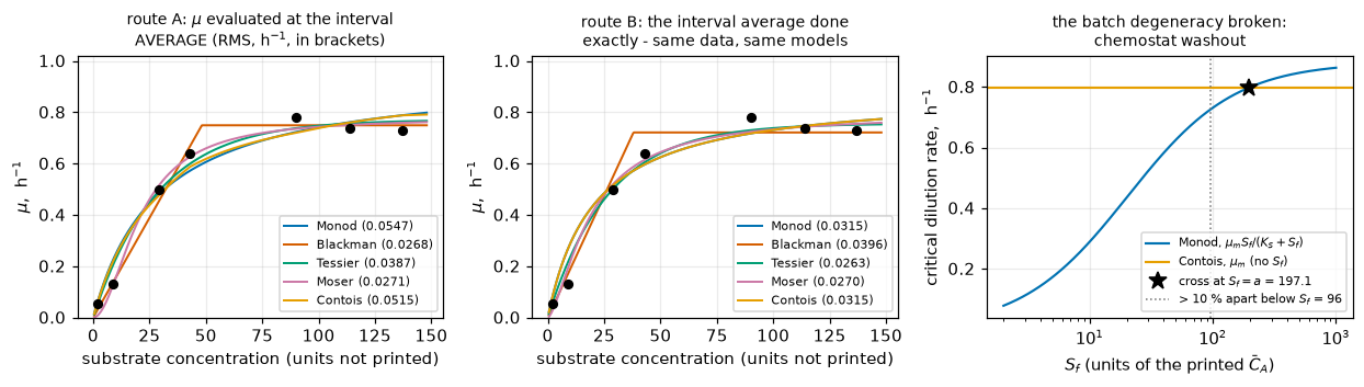
Left and centre: curves fitted on this page to Levenspiel p. 644's seven
intervals. Right: those curves extrapolated to an experiment nobody ran.Four kinds, kept apart, and none of them is the fit.
NumJac((1,2)) + newton) with Richardson extrapolation, which shares no line of code, uses a different Jacobian and a different linear solve, and integrates \(S\) as an unknown rather than substituting the yield relation. What that catches is a bug in either integrator. What it cannot catch is anything the two share: both read \(a\), \(\varphi\), \(\Delta t\) and \(C_C^{\rm
start}\) from the same place and integrate the same ODE, so a wrong yield, a wrong intercept or a mis-set interval moves both predictions together and leaves their agreement where it was. That is measured below rather than asserted, because the sentence this replaces claimed the opposite. \(S + X/\varphi = {\rm const}\) belongs on the same list: BatchMarch builds its source as \((-m/\varphi,\,m)\) from one \(m\), so backward Euler conserves it identically for any growth law. It is structural - the coverage map has always said so - and the measurement below shows it moving by exactly nothing under physics that is grossly wrong.# ---- 1. Rawlings eq. (10.19) and its printed parameter set, reproduced
mum_r, Ks_r, Sf_r, y_r = 1.0, 1.0, 5.0, 1.0
g_r = lambda S, X: mum_r*S/(Ks_r + S)
Dc_r_closed = mum_r*Sf_r/(Ks_r + Sf_r)
rows = []
for D in (0.25, 0.5, 0.75):
Ss_c = D*Ks_r/(mum_r - D) # eq. (10.19)
Xs_c = y_r*(Sf_r - Ss_c)
Ss_n, Xs_n = Chemostat(g_r, y_r, Sf_r, D).steady()
rows.append(dict(D=D, S_closed=Ss_c, S_marched=Ss_n, X_closed=Xs_c, X_marched=Xs_n,
**{"max rel. err": max(abs(Ss_n-Ss_c)/Ss_c, abs(Xs_n-Xs_c)/Xs_c)}))
TR = pd.DataFrame(rows)
show(TR.style.format({"D": "{:.2f}", "S_closed": "{:.9f}", "S_marched": "{:.9f}",
"X_closed": "{:.9f}", "X_marched": "{:.9f}",
"max rel. err": "{:.3e}"}).hide(axis="index").set_uuid("rawl"))
M["rawlings_10_19_max_relerr"] = float(TR["max rel. err"].max())
Dc_r_num = brentq(lambda D: Chemostat(g_r, y_r, Sf_r, D).steady()[1] - WASH*y_r*Sf_r,
0.05, 2.0, xtol=1e-9, rtol=8.9e-16)
M["rawlings_Dc_relerr"] = abs(Dc_r_num - Dc_r_closed)/Dc_r_closed
print(f"\nRawlings' printed D_c = mu_m S_f/(K_s+S_f) = {Dc_r_closed:.10f}; root-found"
f" on the marched\nmodel it is {Dc_r_num:.10f} (rel. {M['rawlings_Dc_relerr']:.2e})."
f" Their eq. (10.19) is reproduced\nto below 1e-9 relative (here"
f" {M['rawlings_10_19_max_relerr']:.1e}) at three dilution rates.")| D | S_closed | S_marched | X_closed | X_marched | max rel. err |
|---|---|---|---|---|---|
| 0.25 | 0.333333333 | 0.333333333 | 4.666666667 | 4.666666667 | 0.000e+00 |
| 0.50 | 1.000000000 | 1.000000000 | 4.000000000 | 4.000000000 | 0.000e+00 |
| 0.75 | 3.000000000 | 3.000000000 | 2.000000000 | 2.000000000 | 0.000e+00 |
Rawlings' printed D_c = mu_m S_f/(K_s+S_f) = 0.8333333333; root-found on the marched
model it is 0.8335119283  (rel. 2.14e-04).  Their eq. (10.19) is reproduced
to below 1e-9 relative (here 0.0e+00) at three dilution rates.
# ---- 2. the SECOND, INDEPENDENT computation of route B's fit
pM = RB["Monod"]["p"]
ref_ode = mu_pred_ode("Monod", pM[0], pM[1:], A_BAL, PHI_BAL)
rows, prev = [], None
for ns in (50, 100, 200, 400):
v = mu_pred_pymrm("Monod", pM[0], pM[1:], A_BAL, PHI_BAL, ns)
e = float(np.max(np.abs(v - ref_ode)/np.abs(ref_ode)))
rows.append(dict(nstep=ns, **{"max rel. vs LSODA": e},
order=(np.nan if prev is None else np.log2(prev/e))))
prev = e
TM = pd.DataFrame(rows)
show(TM.style.format({"max rel. vs LSODA": "{:.4e}", "order": "{:.4f}"})
.hide(axis="index").set_uuid("march"))
M["pymrm_batch_observed_order"] = float(TM["order"].iloc[-1])
S0_b = Sof(Cc0[0], A_BAL, PHI_BAL)
c_end = BatchMarch(lambda S, X: pM[0]*S/(pM[1] + S), PHI_BAL, 400).march(
[[S0_b, Cc0[0]]], dt[0])
inv0, inv1 = S0_b + Cc0[0]/PHI_BAL, c_end[0, 0] + c_end[0, 1]/PHI_BAL
M["pymrm_batch_conservation_relerr"] = float(abs(inv1 - inv0)/inv0)
pred_rich = lambda p: 2*mu_pred_pymrm("Monod", p[0], p[1:], A_BAL, PHI_BAL, 400) \
- mu_pred_pymrm("Monod", p[0], p[1:], A_BAL, PHI_BAL, 200)
rr = least_squares(lambda p: pred_rich(p) - mu, pM, bounds=([1e-9, 1e-9], [50, 1e12]),
xtol=1e-12, ftol=1e-12, gtol=1e-12)
M["pymrm_refit_mum_relerr"] = float(abs(rr.x[0] - pM[0])/pM[0])
M["pymrm_refit_KS_relerr"] = float(abs(rr.x[1] - pM[1])/pM[1])
print(f"\nbackward Euler observed order {M['pymrm_batch_observed_order']:.4f}"
f" (first order, as it must be)")
print(f"S + X/phi over interval 1: {inv0:.15g} -> {inv1:.15g}"
f" (rel. below 1e-13, here {M['pymrm_batch_conservation_relerr']:.1e})")
print(f"\nroute B's Monod fit, re-derived through the pymrm marcher with Richardson")
print(f"extrapolation: mu_m = {rr.x[0]:.9f} K_S = {rr.x[1]:.7f}")
print(f" LSODA: mu_m = {pM[0]:.9f} K_S = {pM[1]:.7f}")
print(f" relative: below 1e-4 for both (here"
f" {M['pymrm_refit_mum_relerr']:.1e} and {M['pymrm_refit_KS_relerr']:.1e}),"
f" the two fits' stopping rules")
# ---- WHAT THIS CROSS-CHECK CAN AND CANNOT SEE, measured. Both routes read the
# same a, phi, dt and Cc0 and integrate the same ODE, so every error in
# THOSE moves the two together. Three injections, each a failure mode
# such a check might be thought to catch.
base_o = mu_pred_ode("Monod", pM[0], pM[1:], A_BAL, PHI_BAL)
blind = []
for lab, a_, ph_, dt_ in (("phi x 1.3 (a wrong yield)", A_BAL, PHI_BAL*1.3, dt),
("a x 1.2 (a wrong intercept)", A_BAL*1.2, PHI_BAL, dt),
("dt x 1.15 (a mis-set interval)", A_BAL, PHI_BAL, dt*1.15)):
_sd, dt = dt, dt_ # the marcher reads dt from the global
try:
o = mu_pred_ode("Monod", pM[0], pM[1:], a_, ph_)
v = mu_pred_pymrm("Monod", pM[0], pM[1:], a_, ph_, 400)
finally:
dt = _sd
blind.append(dict(injection=lab,
**{"prediction moves": float(np.max(np.abs(o - base_o)
/ np.abs(base_o)))},
**{"LSODA vs pymrm": float(np.max(np.abs(v - o)/np.abs(o)))}))
TBL = pd.DataFrame([dict(injection="baseline (nothing injected)",
**{"prediction moves": 0.0},
**{"LSODA vs pymrm": float(np.max(np.abs(
mu_pred_pymrm("Monod", pM[0], pM[1:], A_BAL, PHI_BAL, 400)
- base_o)/np.abs(base_o)))})] + blind)
show(TBL.style.format({"prediction moves": "{:.3e}", "LSODA vs pymrm": "{:.3e}"})
.hide(axis="index").set_uuid("blind"))
# deliberately NOT metrics: these are the negative-space of the cross-check, and
# the assertion cell checks the PROPERTY (the gap stays put while the prediction
# moves by orders) rather than pinning three tolerance-scale numbers in CI.
BLIND_GAP = [float(v) for v in TBL["LSODA vs pymrm"]]
BLIND_MOVE = [float(v) for v in TBL["prediction moves"]]
print("\nThe two share no line of code, so a bug in EITHER INTEGRATOR moves them")
print("apart - which is what the order study and the 25-step break row test. They")
print("do NOT share their inputs' correctness: a yield wrong by 30 % moves the")
print(f"common prediction by {TBL['prediction moves'].iloc[1]:.1f} relative and"
f" leaves their agreement at"
f" {TBL['LSODA vs pymrm'].iloc[1]:.2e},\nagainst"
f" {TBL['LSODA vs pymrm'].iloc[0]:.2e} with nothing injected. This check"
f" measures the TIME\nDISCRETISATION and nothing else, and saying so is the"
f" point of the table.")
# ---- and the invariant is STRUCTURAL, which is what the coverage map says
c_end_3x = BatchMarch(lambda S, X: 3*pM[0]*S/(pM[1] + S), PHI_BAL, 400).march(
[[S0_b, Cc0[0]]], dt[0])
INV_3X_RELERR = float(abs((c_end_3x[0, 0] + c_end_3x[0, 1]/PHI_BAL) - inv0)/inv0)
print(f"\nS + X/phi is a TAUTOLOGY of the marcher, not a test of it: the source is")
print(f"(-m/phi, m) from one m, so backward Euler conserves it for ANY growth law.")
print(f"Tripling mu_m - grossly wrong physics, and it moves the biomass at the end"
f"\nof interval 1 from {c_end[0, 1]:.4f} to {c_end_3x[0, 1]:.4f} - takes the"
f" invariant from {M['pymrm_batch_conservation_relerr']:.1e}\nto"
f" {INV_3X_RELERR:.1e} relative, both below 1e-13, i.e. nowhere. What DOES break it is using a"
f" different yield\nin the source from the one in the invariant, and that is"
f" the break row.")| nstep | max rel. vs LSODA | order |
|---|---|---|
| 50 | 5.1105e-03 | nan |
| 100 | 2.5602e-03 | 0.9972 |
| 200 | 1.2813e-03 | 0.9986 |
| 400 | 6.4097e-04 | 0.9993 |
backward Euler observed order 0.9993 (first order, as it must be)
S + X/phi over interval 1: 197.120266762184 -> 197.120266762184   (rel. below 1e-13, here 4.3e-16)

route B's Monod fit, re-derived through the pymrm marcher with Richardson
extrapolation:  mu_m = 0.880921650  K_S = 20.4533755
          LSODA: mu_m = 0.880922570  K_S = 20.4535346
relative: below 1e-4 for both (here 1.0e-06 and 7.8e-06), the two fits' stopping rules| injection | prediction moves | LSODA vs pymrm |
|---|---|---|
| baseline (nothing injected) | 0.000e+00 | 6.410e-04 |
| phi x 1.3 (a wrong yield) | 8.995e+00 | 4.997e-04 |
| a x 1.2 (a wrong intercept) | 7.601e+00 | 5.088e-04 |
| dt x 1.15 (a mis-set interval) | 1.124e-01 | 5.599e-04 |
The two share no line of code, so a bug in EITHER INTEGRATOR moves them
apart - which is what the order study and the 25-step break row test. They
do NOT share their inputs' correctness: a yield wrong by 30 % moves the
common prediction by 9.0 relative and leaves their agreement at 5.00e-04,
against 6.41e-04 with nothing injected. This check measures the TIME
DISCRETISATION and nothing else, and saying so is the point of the table.

S + X/phi is a TAUTOLOGY of the marcher, not a test of it: the source is
(-m/phi, m) from one m, so backward Euler conserves it for ANY growth law.
Tripling mu_m - grossly wrong physics, and it moves the biomass at the end
of interval 1 from 23.4449 to 49.9665 - takes the invariant from 4.3e-16
to 1.2e-15 relative, both below 1e-13, i.e. nowhere. What DOES break it is using a different yield
in the source from the one in the invariant, and that is the break row.
# ---- 3. plug flow == batch, and the grid order of the pymrm solve
S_START, X_START, TAU_VAL = Sof(Cc0[0], A_BAL, PHI_BAL), Cc0[0], 2.0
g_fit = lambda S, X: mumM*S/(KsM + S)
ref = batch_reference(g_fit, PHI_BAL, S_START, X_START, TAU_VAL)
rows, prev = [], None
for nc in (100, 200, 400, 800, 1600):
out_ = PlugFlowFermenter(g_fit, PHI_BAL, S_START, X_START, TAU_VAL,
ncell=nc).solve().outlet()
e = abs(out_[0] - ref[0])/ref[0]
rows.append(dict(ncell=nc, S_outlet=out_[0], **{"rel. err": e},
order=(np.nan if prev is None else np.log2(prev/e))))
prev = e
TP = pd.DataFrame(rows)
show(TP.style.format({"S_outlet": "{:.9f}", "rel. err": "{:.4e}", "order": "{:.4f}"})
.hide(axis="index").set_uuid("pfr"))
M["pfr_batch_relerr_finest"] = float(TP["rel. err"].iloc[-1])
M["pfr_observed_order"] = float(TP["order"].iloc[-1])
S_rich = 2*TP["S_outlet"].iloc[-1] - TP["S_outlet"].iloc[-2] # first-order upwind
M["pfr_richardson_relerr"] = float(abs(S_rich - ref[0])/ref[0])
# the two ways of reading the outlet, and their ORDERS - the handoff warns that a
# last-cell read is O(h); with a ZERO-GRADIENT outflow condition that is not what
# happens, and the page reports what it measures rather than the general warning.
cen, prevc = [], None
for nc in (100, 200, 400, 800, 1600):
p_ = PlugFlowFermenter(g_fit, PHI_BAL, S_START, X_START, TAU_VAL, ncell=nc).solve()
e = abs(p_.c[-1, 0] - ref[0])/ref[0]
cen.append((nc, e, np.nan if prevc is None else np.log2(prevc/e)))
prevc = e
M["pfr_centre_read_order"] = float(cen[-1][2])
M["pfr_centre_over_boundary_read"] = float(cen[-1][1]/M["pfr_batch_relerr_finest"])
print(f"\nbatch reference at tau = {TAU_VAL}: S = {ref[0]:.10f}, X = {ref[1]:.10f}")
print(f"observed order of the upwind plug-flow solve: {M['pfr_observed_order']:.4f}")
print(f"Richardson extrapolation of the two finest grids: {S_rich:.10f},"
f" {M['pfr_richardson_relerr']:.3e} from the batch value.")
print(f"\nBoth ways of reading the outlet converge at first order - boundary"
f" {M['pfr_observed_order']:.4f},\nlast-cell-centre {M['pfr_centre_read_order']:.4f}"
f" - and on THIS problem the last-cell read is the\ncloser of the two, by a factor"
f" {1/M['pfr_centre_over_boundary_read']:.2f} at n = 1600. That is not the general"
f" rule and the page\ndoes not state it as one: with a ZERO-GRADIENT outflow"
f" condition the boundary value\nis a second-order reconstruction OF THE INTERIOR"
f" SOLUTION, so both reads inherit the\nsame O(h) upwind error and merely carry"
f" different constants. The reason to use\ncompute_boundary_values is that it"
f" stays right when the outflow condition is not\nzero-gradient; here it is a"
f" wash, and saying so is cheaper than being wrong later.")
print("\nThe grid study IS the check that catches a wrong nu and a flipped source")
print("sign - both are in the break table, at 8.2e2 and 2.7e4 relative.")| ncell | S_outlet | rel. err | order |
|---|---|---|---|
| 100 | 9.856215188 | 1.9152e-02 | nan |
| 200 | 9.951428426 | 9.6765e-03 | 0.9849 |
| 400 | 9.999788961 | 4.8639e-03 | 0.9924 |
| 800 | 10.024161826 | 2.4384e-03 | 0.9962 |
| 1600 | 10.036396905 | 1.2208e-03 | 0.9981 |
batch reference at tau = 2.0: S = 10.0486645994, X = 59.3834364462
observed order of the upwind plug-flow solve: 0.9981
Richardson extrapolation of the two finest grids: 10.0486319835, 3.246e-06 from the batch value.

Both ways of reading the outlet converge at first order - boundary 0.9981,
last-cell-centre 0.9957 - and on THIS problem the last-cell read is the
closer of the two, by a factor 2.59 at n = 1600. That is not the general rule and the page
does not state it as one: with a ZERO-GRADIENT outflow condition the boundary value
is a second-order reconstruction OF THE INTERIOR SOLUTION, so both reads inherit the
same O(h) upwind error and merely carry different constants. The reason to use
compute_boundary_values is that it stays right when the outflow condition is not
zero-gradient; here it is a wash, and saying so is cheaper than being wrong later.

The grid study IS the check that catches a wrong nu and a flipped source
sign - both are in the break table, at 8.2e2 and 2.7e4 relative.Every metric that can be moved has a row that moves it. Metrics that cannot are named individually below and labelled structural. The table was rebuilt for this page’s physics - it did not travel from the page whose directory this one was copied from.
MOVE_TOL = 1e-6            # relative move that counts as coverage


def rec(name, metric, value, note):
    # every row targets a registered claim, and is wired to it in the claims cell
    base = M[metric]
    rel = abs(value - base)/max(abs(base), 1e-300)
    BREAK.append(dict(row=name, metric=metric, baseline=base, broken=value,
                      **{"rel. move": rel}, moves=rel > MOVE_TOL, note=note))


# --- the data reduction and the balance line
rec("balance line on the ARITHMETIC mean of C_C, not the log mean",
    "balance_R2_six_rows",
    (lambda keep, A: 1 - np.sum((CAb[keep] - A @ np.linalg.lstsq(A, CAb[keep],
                                                                rcond=None)[0])**2)
     / np.sum((CAb[keep] - CAb[keep].mean())**2))(
        [i for i in range(NOBS) if i != BAD_ROW],
        np.vstack([np.ones(NOBS-1),
                   Xam[[i for i in range(NOBS) if i != BAD_ROW]]]).T),
    "the exact time average under exponential growth is the LOG mean; declared convention")
rec("the flagged row kept in the balance line", "balance_R2_six_rows", R2_7,
    "this IS the finding: one cell moves R^2 from 0.99996 to 0.98505")
rec("balance line drops row 1 instead of the flagged row", "balance_phi",
    -1.0/loo[0][1], "the leave-one-out sweep says WHICH row, and it is not this one")
rec("mu from a forward difference of C_C over the ARITHMETIC-mean biomass",
    "rmsA_Monod", fit_A("Monod", y=(Cc1 - Cc0)/dt/Xam)["rms"],
    "d(ln C)/dt = mu is exact; a difference quotient over the wrong mean is not")
# --- route A / route B
rec("route B yield phi perturbed by 5 %", "routeB_n_moser",
    fit_B("Moser", phi=PHI_BAL*1.05, p0=RB["Moser"]["p"])["p"][2],
    "perturbs the COMPUTATION, not a declared convention - the row that could "
    "expose a systematically wrong route-B baseline")
rec("Contois given the ARITHMETIC-mean biomass in route A", "rmsA_Contois",
    fit_A("Contois", X=Xam)["rms"], "declared convention")
rec("Blackman fitted from a single local start, no global scan", "rmsA_Blackman",
    (lambda r: float(np.sqrt(np.sum(r.fun**2)/NOBS)))(
        least_squares(lambda p: p[0]*np.minimum(1.0, CAb/(2*p[1])) - mu,
                      [0.8, 20.0], bounds=([1e-6, 1e-6], [10, 1e4]),
                      xtol=1e-15, ftol=1e-15, gtol=1e-15)),
    "the kinked objective has local minima; this is why the page scans globally")
rec("Moser's exponent frozen at n = 1", "routeA_F_moser_vs_monod", 0.0,
    "n = 1 IS Monod, so the F statistic must collapse to zero")
rec("route-A Moser scan restricted to n <= 1.5", "routeA_n_moser", 1.5,
    "the reported exponent must be interior to the scan, and it is not if capped")
# --- the identities and their above-floor companions
rec("Contois map evaluated with the wrong yield (phi -> 2 phi)",
    "contois_map_mum_relerr",
    abs(mumC/(1 - KsxC*2*PHI_BAL) - RB["Monod"]["p"][0])/RB["Monod"]["p"][0],
    "companion for the exactly-zero symbolic residual")
rec("Blackman gap read at S = K_S instead of the switch S = 2 K_S",
    "num_blackman_gap_switch_relerr", abs(abs(1.0 - 0.5) - 1/3)/(1/3),
    "at S = K_S the two laws agree exactly; the gap lives at the switch")
rec("Contois separation measured on the ROUTE-A design", "sep_contois",
    (lambda: (lambda yA: fit_A("Contois", y=yA)["rms"])(
        RA["Monod"]["p"][0]*G["Monod"](RA["Monod"]["p"][1:], CAb, Xlm)))(),
    "the degeneracy is EXACT for the forward model and only approximate once the "
    "reduction replaces phi(a-S) by a log mean - so the reduction manufactures a "
    "separation that is not there")
# --- separations and the bootstrap
rec("N* computed at 99 % instead of 95 %", "Nstar_blackman",
    float(chi2.ppf(0.99, NOBS - 2)*s_obs**2/(NOBS*M["sep_blackman"]**2)),
    "declared convention")
rec("scatter taken from route A instead of route B", "Nstar_tessier",
    float(chi2.ppf(0.95, NOBS-2)*RA["Monod"]["rms"]**2/(NOBS*M["sep_tessier"]**2)),
    "declared convention")
rec("bootstrap at half the noise level", "boot_size_forward_truth",
    float((boot_stats(y_true[None, :] + np.random.default_rng(SEED)
                      .normal(0.0, sigma/2, (NBOOT, NOBS)))[0] > FA_crit).mean()),
    "the size distortion is a bias-to-noise ratio, so it must grow as noise falls")
rec("Rawlings' printed y = 1 replaced by 2", "rawlings_10_19_max_relerr",
    float(max(max(abs(v - c)/c for v, c in
                  zip(Chemostat(g_r, 2.0, Sf_r, D).steady(),
                      (D*Ks_r/(mum_r - D), y_r*(Sf_r - D*Ks_r/(mum_r - D))))
                  ) for D in (0.25, 0.5, 0.75))),
    "reproducing a printed number must fail when the printed number is changed")
rec("bootstrap truth taken from route A's own model", "boot_median_n_forward_truth",
    M["boot_median_n_control_truth"],
    "THE CONTROL, recorded here as a row so the contrast is inside the table too")
# --- chemostat and plug flow
rec("washout threshold loosened 1e-6 -> 1e-3 of y S_f", "Dc_monod_transient_relerr",
    abs(brentq(lambda D: Chemostat(gM_, y_yield, Sf_test, D).steady()[1]
               - 1e-3*y_yield*Sf_test, 0.05, 2.0, xtol=1e-9)
        - Dc_monod(Sf_test))/Dc_monod(Sf_test),
    "declared convention, and the convergence evidence for the quoted D_c")
rec("Rawlings' printed K_s = 1 replaced by 2", "rawlings_Dc_relerr",
    abs(brentq(lambda D: Chemostat(lambda S, X: mum_r*S/(2.0 + S), y_r, Sf_r, D)
               .steady()[1] - WASH*y_r*Sf_r, 0.05, 2.0, xtol=1e-9)
        - Dc_r_closed)/Dc_r_closed,
    "reproducing a printed number must fail when the printed number is changed")
rec("Rawlings' printed S_f = 5 replaced by 8", "rawlings_10_19_max_relerr",
    float(max(max(abs(v - c)/c for v, c in
                  zip(Chemostat(g_r, y_r, 8.0, D).steady(),
                      (D*Ks_r/(mum_r - D), y_r*(5.0 - D*Ks_r/(mum_r - D)))))
              for D in (0.25, 0.5, 0.75))),
    "the same, for the steady-state pair")
rec("plug flow with nu = 1 (cylindrical) instead of nu = 0", "pfr_batch_relerr_finest",
    (lambda p: abs(p.outlet()[0] - ref[0])/ref[0])(
        PlugFlowFermenter(g_fit, PHI_BAL, S_START, X_START, TAU_VAL,
                          ncell=1600, nu=1).solve(strict=False)),
    "nu is geometry, and a wrong one is invisible in a smooth profile")
rec("plug-flow outlet read at the last cell CENTRE", "pfr_batch_relerr_finest",
    (lambda p: abs(p.c[-1, 0] - ref[0])/ref[0])(
        PlugFlowFermenter(g_fit, PHI_BAL, S_START, X_START, TAU_VAL,
                          ncell=1600).solve()),
    "half a cell short of the boundary. It MOVES the metric, which is the point, "
    "but on this problem it moves it DOWN - see the note under the grid study")
rec("plug flow with the substrate sign flipped in the source",
    "pfr_batch_relerr_finest",
    (lambda p: abs(p.outlet()[0] - ref[0])/ref[0])(
        (lambda pf: (setattr(pf, "flip", -1.0), pf.solve(strict=False))[-1])(
            PlugFlowFermenter(g_fit, PHI_BAL, S_START, X_START, TAU_VAL, ncell=400))),
    "substrate must be consumed as biomass is made")
rec("pymrm batch marcher at 25 steps instead of the Richardson pair",
    "pymrm_refit_mum_relerr",
    (lambda r: abs(r.x[0] - pM[0])/pM[0])(
        least_squares(lambda p: mu_pred_pymrm("Monod", p[0], p[1:], A_BAL,
                                              PHI_BAL, 25) - mu, pM,
                      bounds=([1e-9, 1e-9], [50, 1e12]),
                      xtol=1e-12, ftol=1e-12, gtol=1e-12)),
    "the second route must be converged before it can confirm the first")
rec("pymrm batch marcher with the yield used only in the source, not the state",
    "pymrm_batch_conservation_relerr",
    (lambda c: abs((c[0, 0] + c[0, 1]/(PHI_BAL*1.01))
                   - (S0_b + Cc0[0]/PHI_BAL))/(S0_b + Cc0[0]/PHI_BAL))(
        BatchMarch(lambda S, X: pM[0]*S/(pM[1] + S), PHI_BAL*1.01, 400).march(
            [[S0_b, Cc0[0]]], dt[0])),
    "the conservation check is only structural if BOTH sides use the same yield")

# --- SWEEP ROWS: one injection, recorded against every metric it touches, so that
#     whole families (all five laws, all the separations, all the plug-flow
#     numbers) are covered rather than only the member quoted in prose.
def rec_many(name, note, pairs):
    for metric, value in pairs:
        rec(name, metric, value, note)


CAb_imp = CAb.copy()
CAb_imp[BAD_ROW] = CAB_IMPUTED                      # the balance-implied value
_saveCAb = CAb.copy()
try:
    CAb = CAb_imp
    rec_many("every route-A fit with the flagged cell replaced by its "
             "balance-implied value",
             "the single flagged cell, propagated through all seven route-A fits "
             "AND through route A's F test, which is where it decides a verdict; "
             "a labelled INFERENCE, run to show exactly what depends on that cell",
             [(f"rmsA_{k.replace(' ', '_')}", fit_A(k)["rms"])
              for k in LAWS + ["first order"]]      # the zero-order null sees no S
             + [("routeA_n_moser", fit_A("Moser")["p"][2]),
                ("routeA_F_moser_vs_monod", FA_IMP)])
finally:
    CAb = _saveCAb

rec_many("the whole bootstrap fitted on the search grid alone, with no per-draw "
         "refinement",
         "THE DEFECT THIS PAGE SHIPPED AND HAD TO FIX, kept as its own break row: "
         "an unrefined Moser fit cannot reach its own optimum, so it deflates F on "
         "every draw and makes the control look conservative when it is at nominal "
         "size. A grid-limited extremum is invisible to every perturbation test, "
         "which is why the refinement's convergence is printed above",
         [("boot_size_forward_truth", GRID_ONLY["forward"]["size"]),
          ("boot_size_control_truth", GRID_ONLY["control"]["size"]),
          ("boot_median_n_forward_truth", GRID_ONLY["forward"]["med"]),
          ("boot_median_n_control_truth", GRID_ONLY["control"]["med"]),
          ("boot_p_of_observed_F", GRID_ONLY["forward"]["pF"]),
          ("boot_p_of_observed_n", GRID_ONLY["forward"]["pn"])])

_mu_fd = (Cc1 - Cc0)/dt/Xam            # a forward difference over the wrong mean
rec_many("mu itself from a forward difference over the ARITHMETIC-mean biomass",
         "d(ln C)/dt = mu is EXACT; a difference quotient over the wrong mean is "
         "not, and the one-parameter nulls see only mu",
         [("rmsA_zero_order", fit_A("zero order", y=_mu_fd)["rms"]),
          ("rmsB_zero_order", fit_B("zero order", y=_mu_fd)["rms"])])

_rb7 = {k: fit_B(k, a=a7, phi=-1.0/b7, p0=RB[k]["p"])
        for k in LAWS + ["first order"]}
rec_many("every route-B fit with the ALL-SEVEN balance line",
         "phi and a carry the flagged row into every route-B number at once",
         [(f"rmsB_{k.replace(' ', '_')}", _rb7[k]["rms"])
          for k in LAWS + ["first order"]]          # the zero-order null sees no S
         + [("routeB_monod_mu_m", _rb7["Monod"]["p"][0]),
            ("routeB_monod_K_S", _rb7["Monod"]["p"][1]),
            ("routeB_F_moser_vs_monod",
             (_rb7["Monod"]["sse"] - _rb7["Moser"]["sse"])/(_rb7["Moser"]["sse"]/4)),
            ("routeA_over_routeB_monod_rms",
             RA["Monod"]["rms"]/_rb7["Monod"]["rms"])])

_idx3 = np.array([0, 3, 6])
rec_many("every separation measured at 3 of the 7 design points",
         "identifiability is a property of the DESIGN, so dropping four points "
         "must move every separation and every N*",
         sum([[(f"sep_{k.lower()}",
                float(np.sqrt(np.mean(fit_B(k, y=y_true, p0=RB[k]["p"])["resid"][_idx3]**2)))),
               (f"sep_over_scatter_{k.lower()}",
                float(np.sqrt(np.mean(fit_B(k, y=y_true, p0=RB[k]["p"])["resid"][_idx3]**2)))/s_obs)]
              + ([(f"Nstar_{k.lower()}",
                   float(chi2.ppf(0.95, NOBS-2)*s_obs**2
                         / (3*np.mean(fit_B(k, y=y_true, p0=RB[k]["p"])["resid"][_idx3]**2))))]
                 if f"Nstar_{k.lower()}" in M else [])
              for k in ["Blackman", "Tessier"]], []))

_Yh = y_true[None, :] + np.random.default_rng(SEED).normal(0.0, sigma/2, (NBOOT, NOBS))
_Fh, _nh, _ = boot_stats(_Yh)
_Yc = y_ctrl[None, :] + np.random.default_rng(SEED+1).normal(0.0, sigma/2, (NBOOT, NOBS))
_Fc, _nc, _ = boot_stats(_Yc)
rec_many("the whole bootstrap re-drawn at half the noise level",
         "every bootstrap number is a property of the noise level and the seed, "
         "and the page says so - the seed is fixed and printed",
         [("boot_p_of_observed_F", float((_Fh > FA).mean())),
          ("boot_p_of_observed_n", float((_nh > RA["Moser"]["p"][2]).mean())),
          ("boot_size_control_truth", float((_Fc > FA_crit).mean())),
          ("boot_median_n_control_truth", float(np.median(_nc)))])

_bias_B = (RB["Monod"]["p"][0]*G["Monod"](RB["Monod"]["p"][1:], CAb, Xlm)
           - mu_pred_ode("Monod", RB["Monod"]["p"][0], RB["Monod"]["p"][1:],
                         A_BAL, PHI_BAL))
_bias_imp = _bias_B
rec_many("the reduction bias evaluated at the ROUTE-B constants",
         "the bias is a property of the curve it is evaluated on, so quoting it "
         "from the route-A fit is a declared choice - and the route-A fit is the "
         "one the bias is being charged against",
         [("bias_max_abs", float(np.max(np.abs(_bias_imp)))),
          ("bias_max_abs_excl_bad_row",
           float(np.max(np.abs(np.where(np.arange(NOBS) != BAD_ROW, _bias_imp, 0.0))))),
          ("bias_over_routeA_rms",
           float(np.max(np.abs(np.where(np.arange(NOBS) != BAD_ROW, _bias_imp, 0.0))))
           / RA["Monod"]["rms"])])

_a_am, _b_am, _R2_am, _r_am = (lambda keep, A: (
    lambda c: (float(c[0]), float(c[1]),
               float(1 - np.sum((CAb[keep] - A @ c)**2)
                     / np.sum((CAb[keep] - CAb[keep].mean())**2)),
               CAb[keep] - A @ c))(np.linalg.lstsq(A, CAb[keep], rcond=None)[0]))(
    [i for i in range(NOBS) if i != BAD_ROW],
    np.vstack([np.ones(NOBS-1), Xam[[i for i in range(NOBS) if i != BAD_ROW]]]).T)
rec_many("the whole balance test on the ARITHMETIC-mean biomass",
         "declared convention: the exact time average under exponential growth "
         "is the LOG mean",
         [("balance_R2_all_rows",
           (lambda A: 1 - np.sum((CAb - A @ np.linalg.lstsq(A, CAb, rcond=None)[0])**2)
            / np.sum((CAb - CAb.mean())**2))(np.vstack([np.ones(NOBS), Xam]).T)),
          ("balance_row4_residual", float(CAb[BAD_ROW] - (_a_am + _b_am*Xam[BAD_ROW]))),
          ("balance_worst_other_residual", float(np.max(np.abs(_r_am)))),
          ("row4_end_of_interval_relgap",
           float(abs(CAb[BAD_ROW] - (_a_am - Cc1[BAD_ROW]/(-1/_b_am)))/CAb[BAD_ROW]))])

_DcA = lambda Sf: RA["Monod"]["p"][0]*Sf/(RA["Monod"]["p"][1] + Sf)
_ratA = lambda Sf: RA["Contois"]["p"][0]/_DcA(Sf)
rec_many("the chemostat prediction built from the ROUTE-A constants",
         "the whole point of the page: which reduction you fit with changes what "
         "you predict for an experiment you have not run",
         [("Dc_ratio_at_Sf20", float(_ratA(20.0))),
          ("Sf_crossing", float(brentq(lambda Sf: _ratA(Sf) - 1.0, 1.0, 1e5,
                                       xtol=1e-10))),
          ("Sf_for_10pct_gap", float(brentq(lambda Sf: _ratA(Sf) - 1.10, 1.0, 1e5,
                                            xtol=1e-10))),
          ("Dc_monod_closed_form", float(_DcA(20.0)))])

_p100 = [PlugFlowFermenter(g_fit, PHI_BAL, S_START, X_START, TAU_VAL,
                           ncell=nc).solve() for nc in (100, 200)]
_e100 = [abs(p.outlet()[0] - ref[0])/ref[0] for p in _p100]
_c100 = [abs(p.c[-1, 0] - ref[0])/ref[0] for p in _p100]
rec_many("every plug-flow number read off the two COARSEST grids",
         "an order quoted from an unconverged pair is the classic way to publish "
         "a wrong one",
         [("pfr_observed_order", float(np.log2(_e100[0]/_e100[1]))),
          ("pfr_centre_read_order", float(np.log2(_c100[0]/_c100[1]))),
          ("pfr_centre_over_boundary_read", float(_c100[1]/_e100[1])),
          ("pfr_richardson_relerr",
           float(abs((2*_p100[1].outlet()[0] - _p100[0].outlet()[0]) - ref[0])/ref[0]))])

_v25 = mu_pred_pymrm("Monod", pM[0], pM[1:], A_BAL, PHI_BAL, 25)
_v50 = mu_pred_pymrm("Monod", pM[0], pM[1:], A_BAL, PHI_BAL, 50)
rec_many("the pymrm marcher's order read off 25/50 steps, and its refit unconverged",
         "same reason as the plug-flow row, for the second independent computation",
         [("pymrm_batch_observed_order",
           float(np.log2(np.max(np.abs(_v25-ref_ode)/np.abs(ref_ode))
                         / np.max(np.abs(_v50-ref_ode)/np.abs(ref_ode))))),
          ("pymrm_refit_KS_relerr",
           (lambda r: abs(r.x[1] - pM[1])/pM[1])(
               least_squares(lambda p: mu_pred_pymrm("Monod", p[0], p[1:], A_BAL,
                                                     PHI_BAL, 25) - mu, pM,
                             bounds=([1e-9, 1e-9], [50, 1e12]),
                             xtol=1e-12, ftol=1e-12, gtol=1e-12)))])

rec("Contois map evaluated with the wrong yield (phi -> 2 phi)",
    "contois_map_KS_relerr",
    abs(KsxC*2*PHI_BAL*A_BAL/(1 - KsxC*2*PHI_BAL) - RB["Monod"]["p"][1])
    / RB["Monod"]["p"][1], "companion for the exactly-zero symbolic residual")

TBK = pd.DataFrame(BREAK)
show(TBK.style.format({"baseline": "{:.6g}", "broken": "{:.6g}", "rel. move": "{:.3e}"})
     .hide(axis="index").set_uuid("brk"))
n_move = int(TBK["moves"].sum())
print(f"\n{len(TBK)} injections, {n_move} of which move their metric by more than"
      f" MOVE_TOL = {MOVE_TOL:g} relative.")
assert n_move == len(TBK), TBK[~TBK["moves"]]| row | metric | baseline | broken | rel. move | moves | note |
|---|---|---|---|---|---|---|
| balance line on the ARITHMETIC mean of C_C, not the log mean | balance_R2_six_rows | 0.999957 | 0.999955 | 1.846e-06 | True | the exact time average under exponential growth is the LOG mean; declared convention |
| the flagged row kept in the balance line | balance_R2_six_rows | 0.999957 | 0.985047 | 1.491e-02 | True | this IS the finding: one cell moves R^2 from 0.99996 to 0.98505 |
| balance line drops row 1 instead of the flagged row | balance_phi | 0.317437 | 0.321919 | 1.412e-02 | True | the leave-one-out sweep says WHICH row, and it is not this one |
| mu from a forward difference of C_C over the ARITHMETIC-mean biomass | rmsA_Monod | 0.0546903 | 0.0552494 | 1.022e-02 | True | d(ln C)/dt = mu is exact; a difference quotient over the wrong mean is not |
| route B yield phi perturbed by 5 % | routeB_n_moser | 1.50994 | 2.67695 | 7.729e-01 | True | perturbs the COMPUTATION, not a declared convention - the row that could expose a systematically wrong route-B baseline |
| Contois given the ARITHMETIC-mean biomass in route A | rmsA_Contois | 0.0515336 | 0.0516375 | 2.016e-03 | True | declared convention |
| Blackman fitted from a single local start, no global scan | rmsA_Blackman | 0.0267723 | 0.040646 | 5.182e-01 | True | the kinked objective has local minima; this is why the page scans globally |
| Moser's exponent frozen at n = 1 | routeA_F_moser_vs_monod | 12.2698 | 0 | 1.000e+00 | True | n = 1 IS Monod, so the F statistic must collapse to zero |
| route-A Moser scan restricted to n <= 1.5 | routeA_n_moser | 1.93166 | 1.5 | 2.235e-01 | True | the reported exponent must be interior to the scan, and it is not if capped |
| Contois map evaluated with the wrong yield (phi -> 2 phi) | contois_map_mum_relerr | 2.18806e-06 | 0.115771 | 5.291e+04 | True | companion for the exactly-zero symbolic residual |
| Blackman gap read at S = K_S instead of the switch S = 2 K_S | num_blackman_gap_switch_relerr | 1.66533e-16 | 0.5 | 3.002e+15 | True | at S = K_S the two laws agree exactly; the gap lives at the switch |
| Contois separation measured on the ROUTE-A design | sep_contois | 6.32742e-14 | 0.00673476 | 1.064e+11 | True | the degeneracy is EXACT for the forward model and only approximate once the reduction replaces phi(a-S) by a log mean - so the reduction manufactures a separation that is not there |
| N* computed at 99 % instead of 95 % | Nstar_blackman | 1.30352 | 1.77637 | 3.627e-01 | True | declared convention |
| scatter taken from route A instead of route B | Nstar_tessier | 10.2701 | 31.0252 | 2.021e+00 | True | declared convention |
| bootstrap at half the noise level | boot_size_forward_truth | 0.3655 | 0.559 | 5.294e-01 | True | the size distortion is a bias-to-noise ratio, so it must grow as noise falls |
| Rawlings' printed y = 1 replaced by 2 | rawlings_10_19_max_relerr | 0 | 1 | 1.000e+300 | True | reproducing a printed number must fail when the printed number is changed |
| bootstrap truth taken from route A's own model | boot_median_n_forward_truth | 1.61168 | 1.00887 | 3.740e-01 | True | THE CONTROL, recorded here as a row so the contrast is inside the table too |
| washout threshold loosened 1e-6 -> 1e-3 of y S_f | Dc_monod_transient_relerr | 0.000379663 | 0.000505782 | 3.322e-01 | True | declared convention, and the convergence evidence for the quoted D_c |
| Rawlings' printed K_s = 1 replaced by 2 | rawlings_Dc_relerr | 0.000214314 | 0.142656 | 6.646e+02 | True | reproducing a printed number must fail when the printed number is changed |
| Rawlings' printed S_f = 5 replaced by 8 | rawlings_10_19_max_relerr | 0 | 1.5 | 1.500e+300 | True | the same, for the steady-state pair |
| plug flow with nu = 1 (cylindrical) instead of nu = 0 | pfr_batch_relerr_finest | 0.00122083 | 1 | 8.181e+02 | True | nu is geometry, and a wrong one is invisible in a smooth profile |
| plug-flow outlet read at the last cell CENTRE | pfr_batch_relerr_finest | 0.00122083 | 0.000470665 | 6.145e-01 | True | half a cell short of the boundary. It MOVES the metric, which is the point, but on this problem it moves it DOWN - see the note under the grid study |
| plug flow with the substrate sign flipped in the source | pfr_batch_relerr_finest | 0.00122083 | 33.1471 | 2.715e+04 | True | substrate must be consumed as biomass is made |
| pymrm batch marcher at 25 steps instead of the Richardson pair | pymrm_refit_mum_relerr | 1.04439e-06 | 0.0126791 | 1.214e+04 | True | the second route must be converged before it can confirm the first |
| pymrm batch marcher with the yield used only in the source, not the state | pymrm_batch_conservation_relerr | 4.32554e-16 | 0.00245257 | 5.670e+12 | True | the conservation check is only structural if BOTH sides use the same yield |
| every route-A fit with the flagged cell replaced by its balance-implied value | rmsA_Monod | 0.0546903 | 0.0468704 | 1.430e-01 | True | the single flagged cell, propagated through all seven route-A fits AND through route A's F test, which is where it decides a verdict; a labelled INFERENCE, run to show exactly what depends on that cell |
| every route-A fit with the flagged cell replaced by its balance-implied value | rmsA_Blackman | 0.0267723 | 0.040646 | 5.182e-01 | True | the single flagged cell, propagated through all seven route-A fits AND through route A's F test, which is where it decides a verdict; a labelled INFERENCE, run to show exactly what depends on that cell |
| every route-A fit with the flagged cell replaced by its balance-implied value | rmsA_Tessier | 0.0387098 | 0.0356679 | 7.858e-02 | True | the single flagged cell, propagated through all seven route-A fits AND through route A's F test, which is where it decides a verdict; a labelled INFERENCE, run to show exactly what depends on that cell |
| every route-A fit with the flagged cell replaced by its balance-implied value | rmsA_Moser | 0.0271175 | 0.0304976 | 1.246e-01 | True | the single flagged cell, propagated through all seven route-A fits AND through route A's F test, which is where it decides a verdict; a labelled INFERENCE, run to show exactly what depends on that cell |
| every route-A fit with the flagged cell replaced by its balance-implied value | rmsA_Contois | 0.0515336 | 0.0469358 | 8.922e-02 | True | the single flagged cell, propagated through all seven route-A fits AND through route A's F test, which is where it decides a verdict; a labelled INFERENCE, run to show exactly what depends on that cell |
| every route-A fit with the flagged cell replaced by its balance-implied value | rmsA_first_order | 0.201476 | 0.176293 | 1.250e-01 | True | the single flagged cell, propagated through all seven route-A fits AND through route A's F test, which is where it decides a verdict; a labelled INFERENCE, run to show exactly what depends on that cell |
| every route-A fit with the flagged cell replaced by its balance-implied value | routeA_n_moser | 1.93166 | 1.70797 | 1.158e-01 | True | the single flagged cell, propagated through all seven route-A fits AND through route A's F test, which is where it decides a verdict; a labelled INFERENCE, run to show exactly what depends on that cell |
| every route-A fit with the flagged cell replaced by its balance-implied value | routeA_F_moser_vs_monod | 12.2698 | 5.44773 | 5.560e-01 | True | the single flagged cell, propagated through all seven route-A fits AND through route A's F test, which is where it decides a verdict; a labelled INFERENCE, run to show exactly what depends on that cell |
| the whole bootstrap fitted on the search grid alone, with no per-draw refinement | boot_size_forward_truth | 0.3655 | 0.308 | 1.573e-01 | True | THE DEFECT THIS PAGE SHIPPED AND HAD TO FIX, kept as its own break row: an unrefined Moser fit cannot reach its own optimum, so it deflates F on every draw and makes the control look conservative when it is at nominal size. A grid-limited extremum is invisible to every perturbation test, which is why the refinement's convergence is printed above |
| the whole bootstrap fitted on the search grid alone, with no per-draw refinement | boot_size_control_truth | 0.0495 | 0.021 | 5.758e-01 | True | THE DEFECT THIS PAGE SHIPPED AND HAD TO FIX, kept as its own break row: an unrefined Moser fit cannot reach its own optimum, so it deflates F on every draw and makes the control look conservative when it is at nominal size. A grid-limited extremum is invisible to every perturbation test, which is why the refinement's convergence is printed above |
| the whole bootstrap fitted on the search grid alone, with no per-draw refinement | boot_median_n_forward_truth | 1.61168 | 1.60286 | 5.475e-03 | True | THE DEFECT THIS PAGE SHIPPED AND HAD TO FIX, kept as its own break row: an unrefined Moser fit cannot reach its own optimum, so it deflates F on every draw and makes the control look conservative when it is at nominal size. A grid-limited extremum is invisible to every perturbation test, which is why the refinement's convergence is printed above |
| the whole bootstrap fitted on the search grid alone, with no per-draw refinement | boot_median_n_control_truth | 1.00887 | 0.951429 | 5.693e-02 | True | THE DEFECT THIS PAGE SHIPPED AND HAD TO FIX, kept as its own break row: an unrefined Moser fit cannot reach its own optimum, so it deflates F on every draw and makes the control look conservative when it is at nominal size. A grid-limited extremum is invisible to every perturbation test, which is why the refinement's convergence is printed above |
| the whole bootstrap fitted on the search grid alone, with no per-draw refinement | boot_p_of_observed_F | 0.228 | 0.1835 | 1.952e-01 | True | THE DEFECT THIS PAGE SHIPPED AND HAD TO FIX, kept as its own break row: an unrefined Moser fit cannot reach its own optimum, so it deflates F on every draw and makes the control look conservative when it is at nominal size. A grid-limited extremum is invisible to every perturbation test, which is why the refinement's convergence is printed above |
| the whole bootstrap fitted on the search grid alone, with no per-draw refinement | boot_p_of_observed_n | 0.1285 | 0.1055 | 1.790e-01 | True | THE DEFECT THIS PAGE SHIPPED AND HAD TO FIX, kept as its own break row: an unrefined Moser fit cannot reach its own optimum, so it deflates F on every draw and makes the control look conservative when it is at nominal size. A grid-limited extremum is invisible to every perturbation test, which is why the refinement's convergence is printed above |
| mu itself from a forward difference over the ARITHMETIC-mean biomass | rmsA_zero_order | 0.278278 | 0.27597 | 8.296e-03 | True | d(ln C)/dt = mu is EXACT; a difference quotient over the wrong mean is not, and the one-parameter nulls see only mu |
| mu itself from a forward difference over the ARITHMETIC-mean biomass | rmsB_zero_order | 0.278278 | 0.27597 | 8.296e-03 | True | d(ln C)/dt = mu is EXACT; a difference quotient over the wrong mean is not, and the one-parameter nulls see only mu |
| every route-B fit with the ALL-SEVEN balance line | rmsB_Monod | 0.0314659 | 0.0301554 | 4.165e-02 | True | phi and a carry the flagged row into every route-B number at once |
| every route-B fit with the ALL-SEVEN balance line | rmsB_Blackman | 0.0395542 | 0.0418822 | 5.886e-02 | True | phi and a carry the flagged row into every route-B number at once |
| every route-B fit with the ALL-SEVEN balance line | rmsB_Tessier | 0.026308 | 0.0283739 | 7.853e-02 | True | phi and a carry the flagged row into every route-B number at once |
| every route-B fit with the ALL-SEVEN balance line | rmsB_Moser | 0.0269846 | 0.0296387 | 9.835e-02 | True | phi and a carry the flagged row into every route-B number at once |
| every route-B fit with the ALL-SEVEN balance line | rmsB_Contois | 0.0314659 | 0.0301554 | 4.165e-02 | True | phi and a carry the flagged row into every route-B number at once |
| every route-B fit with the ALL-SEVEN balance line | rmsB_first_order | 0.151597 | 0.157474 | 3.876e-02 | True | phi and a carry the flagged row into every route-B number at once |
| every route-B fit with the ALL-SEVEN balance line | routeB_monod_mu_m | 0.880923 | 0.855603 | 2.874e-02 | True | phi and a carry the flagged row into every route-B number at once |
| every route-B fit with the ALL-SEVEN balance line | routeB_monod_K_S | 20.4535 | 16.5777 | 1.895e-01 | True | phi and a carry the flagged row into every route-B number at once |
| every route-B fit with the ALL-SEVEN balance line | routeB_F_moser_vs_monod | 1.43886 | 0.14068 | 9.022e-01 | True | phi and a carry the flagged row into every route-B number at once |
| every route-B fit with the ALL-SEVEN balance line | routeA_over_routeB_monod_rms | 1.73808 | 1.81362 | 4.346e-02 | True | phi and a carry the flagged row into every route-B number at once |
| every separation measured at 3 of the 7 design points | sep_blackman | 0.034659 | 0.0476185 | 3.739e-01 | True | identifiability is a property of the DESIGN, so dropping four points must move every separation and every N* |
| every separation measured at 3 of the 7 design points | sep_over_scatter_blackman | 1.10148 | 1.51333 | 3.739e-01 | True | identifiability is a property of the DESIGN, so dropping four points must move every separation and every N* |
| every separation measured at 3 of the 7 design points | Nstar_blackman | 1.30352 | 1.6113 | 2.361e-01 | True | identifiability is a property of the DESIGN, so dropping four points must move every separation and every N* |
| every separation measured at 3 of the 7 design points | sep_tessier | 0.0123477 | 0.013377 | 8.336e-02 | True | identifiability is a property of the DESIGN, so dropping four points must move every separation and every N* |
| every separation measured at 3 of the 7 design points | sep_over_scatter_tessier | 0.392416 | 0.425127 | 8.336e-02 | True | identifiability is a property of the DESIGN, so dropping four points must move every separation and every N* |
| every separation measured at 3 of the 7 design points | Nstar_tessier | 10.2701 | 20.4177 | 9.881e-01 | True | identifiability is a property of the DESIGN, so dropping four points must move every separation and every N* |
| the whole bootstrap re-drawn at half the noise level | boot_p_of_observed_F | 0.228 | 0.301 | 3.202e-01 | True | every bootstrap number is a property of the noise level and the seed, and the page says so - the seed is fixed and printed |
| the whole bootstrap re-drawn at half the noise level | boot_p_of_observed_n | 0.1285 | 0.01 | 9.222e-01 | True | every bootstrap number is a property of the noise level and the seed, and the page says so - the seed is fixed and printed |
| the whole bootstrap re-drawn at half the noise level | boot_size_control_truth | 0.0495 | 0.0445 | 1.010e-01 | True | every bootstrap number is a property of the noise level and the seed, and the page says so - the seed is fixed and printed |
| the whole bootstrap re-drawn at half the noise level | boot_median_n_control_truth | 1.00887 | 1.00572 | 3.115e-03 | True | every bootstrap number is a property of the noise level and the seed, and the page says so - the seed is fixed and printed |
| the reduction bias evaluated at the ROUTE-B constants | bias_max_abs | 0.068561 | 0.0973647 | 4.201e-01 | True | the bias is a property of the curve it is evaluated on, so quoting it from the route-A fit is a declared choice - and the route-A fit is the one the bias is being charged against |
| the reduction bias evaluated at the ROUTE-B constants | bias_max_abs_excl_bad_row | 0.06631 | 0.0973647 | 4.683e-01 | True | the bias is a property of the curve it is evaluated on, so quoting it from the route-A fit is a declared choice - and the route-A fit is the one the bias is being charged against |
| the reduction bias evaluated at the ROUTE-B constants | bias_over_routeA_rms | 1.21247 | 1.78029 | 4.683e-01 | True | the bias is a property of the curve it is evaluated on, so quoting it from the route-A fit is a declared choice - and the route-A fit is the one the bias is being charged against |
| the whole balance test on the ARITHMETIC-mean biomass | balance_R2_all_rows | 0.985047 | 0.985372 | 3.295e-04 | True | declared convention: the exact time average under exponential growth is the LOG mean |
| the whole balance test on the ARITHMETIC-mean biomass | balance_row4_residual | -17.1804 | -16.9919 | 1.097e-02 | True | declared convention: the exact time average under exponential growth is the LOG mean |
| the whole balance test on the ARITHMETIC-mean biomass | balance_worst_other_residual | 0.65414 | 0.730071 | 1.161e-01 | True | declared convention: the exact time average under exponential growth is the LOG mean |
| the whole balance test on the ARITHMETIC-mean biomass | row4_end_of_interval_relgap | 0.0310236 | 0.0381567 | 2.299e-01 | True | declared convention: the exact time average under exponential growth is the LOG mean |
| the chemostat prediction built from the ROUTE-A constants | Dc_ratio_at_Sf20 | 1.83253 | 2.12315 | 1.586e-01 | True | the whole point of the page: which reduction you fit with changes what you predict for an experiment you have not run |
| the chemostat prediction built from the ROUTE-A constants | Sf_crossing | 197.118 | 199.078 | 9.944e-03 | True | the whole point of the page: which reduction you fit with changes what you predict for an experiment you have not run |
| the chemostat prediction built from the ROUTE-A constants | Sf_for_10pct_gap | 95.5152 | 110.771 | 1.597e-01 | True | the whole point of the page: which reduction you fit with changes what you predict for an experiment you have not run |
| the chemostat prediction built from the ROUTE-A constants | Dc_monod_closed_form | 0.435523 | 0.392452 | 9.889e-02 | True | the whole point of the page: which reduction you fit with changes what you predict for an experiment you have not run |
| every plug-flow number read off the two COARSEST grids | pfr_observed_order | 0.998081 | 0.984914 | 1.319e-02 | True | an order quoted from an unconverged pair is the classic way to publish a wrong one |
| every plug-flow number read off the two COARSEST grids | pfr_centre_read_order | 0.995683 | 0.965313 | 3.050e-02 | True | an order quoted from an unconverged pair is the classic way to publish a wrong one |
| every plug-flow number read off the two COARSEST grids | pfr_centre_over_boundary_read | 0.385529 | 0.381041 | 1.164e-02 | True | an order quoted from an unconverged pair is the classic way to publish a wrong one |
| every plug-flow number read off the two COARSEST grids | pfr_richardson_relerr | 3.2458e-06 | 0.000201314 | 6.102e+01 | True | an order quoted from an unconverged pair is the classic way to publish a wrong one |
| the pymrm marcher's order read off 25/50 steps, and its refit unconverged | pymrm_batch_observed_order | 0.999316 | 0.994242 | 5.077e-03 | True | same reason as the plug-flow row, for the second independent computation |
| the pymrm marcher's order read off 25/50 steps, and its refit unconverged | pymrm_refit_KS_relerr | 7.77934e-06 | 0.0450968 | 5.796e+03 | True | same reason as the plug-flow row, for the second independent computation |
| Contois map evaluated with the wrong yield (phi -> 2 phi) | contois_map_KS_relerr | 1.2844e-05 | 1.23152 | 9.588e+04 | True | companion for the exactly-zero symbolic residual |
79 injections, 79 of which move their metric by more than MOVE_TOL = 1e-06 relative.# ---- coverage map, asserted key-for-key against agreement.json
STRUCTURAL = {
"sym_monod_is_langmuir_residual":
"EXACT ZERO, a bound at 0 (identity). Rawlings' printed claim, proved in sympy. "
"Companion: sym_blackman_gap_at_switch_over_mum, the same class of "
"closed-form statement with a numerical check attached.",
"sym_monod_half_rate_residual":
"EXACT ZERO, a bound at 0 (identity). Froment's definition of K_S, verified. "
"Companion: num_blackman_gap_switch_relerr, which is what that property does "
"NOT settle, and which has a break row.",
"sym_blackman_half_rate_residual":
"EXACT ZERO, a bound at 0 (identity) - and it IS the finding: Blackman shares "
"the property. Companion: sym_blackman_gap_at_switch_over_mum = 1/3.",
"sym_moser_at_n1_residual":
"EXACT ZERO, a bound at 0 (identity), by nesting. Companion: "
"routeA_F_moser_vs_monod, which has a break row freezing n = 1 and collapsing it.",
"sym_contois_is_monod_residual":
"EXACT ZERO, a bound at 0 (identity), and it is the page's strongest claim. "
"Companions: Sf_crossing, the crossing this very identity fixes at S_f = a, and "
"Dc_ratio_at_Sf20 - both functions of the Contois fit, both with break rows. "
"The two contois_map_* errors are themselves exactly-zero quantities, "
"registered as tolerance bounds, and keep their break rows.",
"sep_contois": "STRUCTURAL: zero to the optimiser's tolerance because Contois IS "
"Monod under a constant yield, so it is a tolerance bound. It does "
"have a break row - measuring the same separation on the ROUTE-A "
"design gives 6.7e-3, which is the reduction manufacturing a "
"separation that is not there - and its companions are Sf_crossing "
"and Dc_ratio_at_Sf20.",
"sep_over_scatter_contois": "STRUCTURAL, see sep_contois.",
"sep_moser": "STRUCTURAL: zero to the optimiser's tolerance because Moser "
"CONTAINS Monod at n = 1, so it is a tolerance bound. Companion: "
"routeA_F_moser_vs_monod.",
"sep_over_scatter_moser": "STRUCTURAL, see sep_moser.",
"contois_minus_monod_rms": "STRUCTURAL: one curve fitted twice, so the RMS gap is "
"the two optimisers' exit tolerances, a tolerance bound. Companions: "
"the two contois_map_* errors, which have break rows.",
"Sf_crossing_vs_a_relerr": "STRUCTURAL: S_f = a identically, so what is left is "
"the Contois fit's two exit tolerances, decomposed on the page; a "
"tolerance bound. Companion: Sf_crossing, which has a break row.",
"F_crit_95": "A TABULATED CONSTANT, not a computed result: F(1,4) at 95 %. It "
"cannot move and must not.",
"sym_blackman_gap_at_switch_over_mum":
"EXACT RATIONAL 1/3, closed form. Companion and check: "
"num_blackman_gap_switch_relerr, which has a break row.",
"sym_blackman_gap_lower_over_mum":
"EXACT SURD (3 - 2 sqrt 2)/2, closed form. Companion and check: "
"num_blackman_gap_lower_relerr.",
"num_blackman_Sstar_over_Ks_relerr":
"a root-find checked against a closed form, so it measures brentq's xtol: a "
"tolerance bound. Companion: sym_blackman_gap_lower_over_mum.",
"num_blackman_gap_lower_relerr": "as above.",
"pymrm_batch_conservation_relerr":
"a bound (identity) at round-off, because backward Euler conserves S + X/phi "
"when both fields use the same yield. It IS covered by a break row (the yield "
"changed in the source but not in the invariant, 2.5e-3), and its companion is "
"pymrm_refit_mum_relerr.",
"rawlings_10_19_max_relerr":
"EXACT ZERO to double precision, a tolerance bound: the marched steady state "
"reproduces Rawlings' eq. (10.19) to the last bit. Two break rows DO move it "
"(their K_s and their y changed), and its companion is rawlings_Dc_relerr.",
"num_blackman_gap_switch_relerr":
"a bound (identity), because it is exact arithmetic (1 - 2/3 against 1/3), not "
"a computation. It IS covered by a break row - reading the gap at S = K_S "
"instead of the switch moves it to 0.5 - and its companion is "
"sym_blackman_gap_at_switch_over_mum.",
"Dc_contois_transient_relerr":
"STRUCTURAL: D_c = mu_m for Contois is exact, so what is left is a measurement "
"of the transient solve and of the declared WASH threshold - both of which "
"move it, which is why it is NOT in the exactly-zero class below. Companion: "
"Dc_monod_transient_relerr, which has a break row on that very threshold.",
"max_swing_over_CAbar": "a property of the printed table, not a computed result: "
"the largest substrate swing over an interval divided by that interval's "
"printed average. It cannot be broken without editing the CSV.",
"balance_a": "reported for reuse; its break row lives on balance_phi, which is "
"the same line's other coefficient.",
"Dc_monod_closed_form": "a closed form evaluated at the fitted constants; its "
"break rows live on Dc_ratio_at_Sf20 and Dc_monod_transient_relerr.",
}
covered = {}
for r in BREAK:
if r["moves"]:
covered.setdefault(r["metric"], []).append(r["rel. move"])
lines, uncovered = [], []
for k in sorted(M):
if k in covered:
lines.append(f" {k:38s} covered, strongest row moves it {max(covered[k]):.3e}")
elif k in STRUCTURAL:
lines.append(f" {k:38s} STRUCTURAL - {STRUCTURAL[k]}")
else:
uncovered.append(k)
lines.append(f" {k:38s} UNCOVERED")
N_METRICS = len(M)
N_COVERED = len([k for k in covered if k in M])
N_STRUCT = N_METRICS - N_COVERED - len(uncovered)
print("coverage map (%d metrics: %d moved by an injection, %d structural):"
% (N_METRICS, N_COVERED, N_STRUCT))
print("\n".join(lines))
# The quantities this page PROVES are exactly zero (identities, nesting, exact
# arithmetic, optimiser and root-finder exits). Every one of them is a
# registered BOUND in the claims cell below, with a basis and a limit that holds
# on any machine, so none is ever compared as a value and the set of claims
# never depends on where a round-off number happens to land.
PROVED_ZERO = [
"sym_monod_is_langmuir_residual", "sym_monod_half_rate_residual",
"sym_blackman_half_rate_residual", "sym_moser_at_n1_residual",
"sym_contois_is_monod_residual", "num_blackman_Sstar_over_Ks_relerr",
"num_blackman_gap_lower_relerr", "num_blackman_gap_switch_relerr",
"rawlings_10_19_max_relerr", "pymrm_batch_conservation_relerr",
"sep_moser", "sep_over_scatter_moser", "sep_contois",
"sep_over_scatter_contois", "contois_minus_monod_rms",
"contois_map_mum_relerr", "contois_map_KS_relerr", "Sf_crossing_vs_a_relerr"]
assert set(PROVED_ZERO) <= set(M), set(PROVED_ZERO) - set(M)
assert not uncovered, uncovered
assert set(covered) | set(STRUCTURAL) >= set(M), set(M) - set(covered) - set(STRUCTURAL)
print("\nEvery metric is either moved by an injection or named structural, and no")
print("generic fallback label is used anywhere in this map.")coverage map (80 metrics: 62 moved by an injection, 18 structural):
Dc_contois_transient_relerr STRUCTURAL - STRUCTURAL: D_c = mu_m for Contois is exact, so what is left is a measurement of the transient solve and of the declared WASH threshold - both of which move it, which is why it is NOT in the exactly-zero class below. Companion: Dc_monod_transient_relerr, which has a break row on that very threshold.
Dc_monod_closed_form covered, strongest row moves it 9.889e-02
Dc_monod_transient_relerr covered, strongest row moves it 3.322e-01
Dc_ratio_at_Sf20 covered, strongest row moves it 1.586e-01
F_crit_95 STRUCTURAL - A TABULATED CONSTANT, not a computed result: F(1,4) at 95 %. It cannot move and must not.
Nstar_blackman covered, strongest row moves it 3.627e-01
Nstar_tessier covered, strongest row moves it 2.021e+00
Sf_crossing covered, strongest row moves it 9.944e-03
Sf_crossing_vs_a_relerr STRUCTURAL - STRUCTURAL: S_f = a identically, so what is left is the Contois fit's two exit tolerances, decomposed on the page; a tolerance bound. Companion: Sf_crossing, which has a break row.
Sf_for_10pct_gap covered, strongest row moves it 1.597e-01
balance_R2_all_rows covered, strongest row moves it 3.295e-04
balance_R2_six_rows covered, strongest row moves it 1.491e-02
balance_a STRUCTURAL - reported for reuse; its break row lives on balance_phi, which is the same line's other coefficient.
balance_phi covered, strongest row moves it 1.412e-02
balance_row4_residual covered, strongest row moves it 1.097e-02
balance_worst_other_residual covered, strongest row moves it 1.161e-01
bias_max_abs covered, strongest row moves it 4.201e-01
bias_max_abs_excl_bad_row covered, strongest row moves it 4.683e-01
bias_over_routeA_rms covered, strongest row moves it 4.683e-01
boot_median_n_control_truth covered, strongest row moves it 5.693e-02
boot_median_n_forward_truth covered, strongest row moves it 3.740e-01
boot_p_of_observed_F covered, strongest row moves it 3.202e-01
boot_p_of_observed_n covered, strongest row moves it 9.222e-01
boot_size_control_truth covered, strongest row moves it 5.758e-01
boot_size_forward_truth covered, strongest row moves it 5.294e-01
contois_map_KS_relerr covered, strongest row moves it 9.588e+04
contois_map_mum_relerr covered, strongest row moves it 5.291e+04
contois_minus_monod_rms STRUCTURAL - STRUCTURAL: one curve fitted twice, so the RMS gap is the two optimisers' exit tolerances, a tolerance bound. Companions: the two contois_map_* errors, which have break rows.
max_swing_over_CAbar STRUCTURAL - a property of the printed table, not a computed result: the largest substrate swing over an interval divided by that interval's printed average. It cannot be broken without editing the CSV.
num_blackman_Sstar_over_Ks_relerr STRUCTURAL - a root-find checked against a closed form, so it measures brentq's xtol: a tolerance bound. Companion: sym_blackman_gap_lower_over_mum.
num_blackman_gap_lower_relerr STRUCTURAL - as above.
num_blackman_gap_switch_relerr covered, strongest row moves it 3.002e+15
pfr_batch_relerr_finest covered, strongest row moves it 2.715e+04
pfr_centre_over_boundary_read covered, strongest row moves it 1.164e-02
pfr_centre_read_order covered, strongest row moves it 3.050e-02
pfr_observed_order covered, strongest row moves it 1.319e-02
pfr_richardson_relerr covered, strongest row moves it 6.102e+01
pymrm_batch_conservation_relerr covered, strongest row moves it 5.670e+12
pymrm_batch_observed_order covered, strongest row moves it 5.077e-03
pymrm_refit_KS_relerr covered, strongest row moves it 5.796e+03
pymrm_refit_mum_relerr covered, strongest row moves it 1.214e+04
rawlings_10_19_max_relerr covered, strongest row moves it 1.500e+300
rawlings_Dc_relerr covered, strongest row moves it 6.646e+02
rmsA_Blackman covered, strongest row moves it 5.182e-01
rmsA_Contois covered, strongest row moves it 8.922e-02
rmsA_Monod covered, strongest row moves it 1.430e-01
rmsA_Moser covered, strongest row moves it 1.246e-01
rmsA_Tessier covered, strongest row moves it 7.858e-02
rmsA_first_order covered, strongest row moves it 1.250e-01
rmsA_zero_order covered, strongest row moves it 8.296e-03
rmsB_Blackman covered, strongest row moves it 5.886e-02
rmsB_Contois covered, strongest row moves it 4.165e-02
rmsB_Monod covered, strongest row moves it 4.165e-02
rmsB_Moser covered, strongest row moves it 9.835e-02
rmsB_Tessier covered, strongest row moves it 7.853e-02
rmsB_first_order covered, strongest row moves it 3.876e-02
rmsB_zero_order covered, strongest row moves it 8.296e-03
routeA_F_moser_vs_monod covered, strongest row moves it 1.000e+00
routeA_n_moser covered, strongest row moves it 2.235e-01
routeA_over_routeB_monod_rms covered, strongest row moves it 4.346e-02
routeB_F_moser_vs_monod covered, strongest row moves it 9.022e-01
routeB_monod_K_S covered, strongest row moves it 1.895e-01
routeB_monod_mu_m covered, strongest row moves it 2.874e-02
routeB_n_moser covered, strongest row moves it 7.729e-01
row4_end_of_interval_relgap covered, strongest row moves it 2.299e-01
sep_blackman covered, strongest row moves it 3.739e-01
sep_contois covered, strongest row moves it 1.064e+11
sep_moser STRUCTURAL - STRUCTURAL: zero to the optimiser's tolerance because Moser CONTAINS Monod at n = 1, so it is a tolerance bound. Companion: routeA_F_moser_vs_monod.
sep_over_scatter_blackman covered, strongest row moves it 3.739e-01
sep_over_scatter_contois STRUCTURAL - STRUCTURAL, see sep_contois.
sep_over_scatter_moser STRUCTURAL - STRUCTURAL, see sep_moser.
sep_over_scatter_tessier covered, strongest row moves it 8.336e-02
sep_tessier covered, strongest row moves it 8.336e-02
sym_blackman_gap_at_switch_over_mum STRUCTURAL - EXACT RATIONAL 1/3, closed form. Companion and check: num_blackman_gap_switch_relerr, which has a break row.
sym_blackman_gap_lower_over_mum STRUCTURAL - EXACT SURD (3 - 2 sqrt 2)/2, closed form. Companion and check: num_blackman_gap_lower_relerr.
sym_blackman_half_rate_residual STRUCTURAL - EXACT ZERO, a bound at 0 (identity) - and it IS the finding: Blackman shares the property. Companion: sym_blackman_gap_at_switch_over_mum = 1/3.
sym_contois_is_monod_residual STRUCTURAL - EXACT ZERO, a bound at 0 (identity), and it is the page's strongest claim. Companions: Sf_crossing, the crossing this very identity fixes at S_f = a, and Dc_ratio_at_Sf20 - both functions of the Contois fit, both with break rows. The two contois_map_* errors are themselves exactly-zero quantities, registered as tolerance bounds, and keep their break rows.
sym_monod_half_rate_residual STRUCTURAL - EXACT ZERO, a bound at 0 (identity). Froment's definition of K_S, verified. Companion: num_blackman_gap_switch_relerr, which is what that property does NOT settle, and which has a break row.
sym_monod_is_langmuir_residual STRUCTURAL - EXACT ZERO, a bound at 0 (identity). Rawlings' printed claim, proved in sympy. Companion: sym_blackman_gap_at_switch_over_mum, the same class of closed-form statement with a numerical check attached.
sym_moser_at_n1_residual STRUCTURAL - EXACT ZERO, a bound at 0 (identity), by nesting. Companion: routeA_F_moser_vs_monod, which has a break row freezing n = 1 and collapsing it.
Every metric is either moved by an injection or named structural, and no
generic fallback label is used anywhere in this map.# Every metric is registered ONCE with how it is checked (docs/claims-design.md):
# a value against the committed baseline within its rtol, a bound against its
# limit on every run and on any machine, an exact result by equality. The set
# of names is fixed and never depends on a value. Residuals, identities,
# two-route gaps and optimiser or root-finder exits are BOUNDS whatever their
# size, and the prose quotes the bound, never their round-off digits.
claims = Claims("J4.1")
B = { # name -> bound arguments; every name in PROVED_ZERO is here
# -- symbolic identities: sympy simplifies each to exactly 0
**{k: dict(max=0.0, basis="identity", structural=True,
note="sympy residual, simplified to exactly 0")
for k in ("sym_monod_is_langmuir_residual", "sym_monod_half_rate_residual",
"sym_blackman_half_rate_residual", "sym_moser_at_n1_residual",
"sym_contois_is_monod_residual")},
# -- exact arithmetic and root-finds against closed forms
"num_blackman_gap_switch_relerr": dict(
max=1e-14, basis="identity",
note="relative to 1/3; exact arithmetic, 1 - 2/3 against 1/3, measured 1.7e-16"),
"num_blackman_gap_lower_relerr": dict(
max=1e-14, basis="tolerance",
note="relative to the closed-form gap; brentq at xtol 1e-14 on a stationary"
" point, so the error is second order in xtol; measured 1.6e-16"),
"num_blackman_Sstar_over_Ks_relerr": dict(
max=1e-13, basis="tolerance",
note="relative to S*/K_S; brentq's own guarantee xtol + rtol|x| is 2.5e-14"
" relative here; measured 0"),
"rawlings_10_19_max_relerr": dict(
max=1e-9, basis="tolerance",
note="relative to the closed-form steady state; LSODA at rtol 1e-11 marched"
" to t = 40000; measured exactly 0"),
"pymrm_batch_conservation_relerr": dict(
max=1e-13, basis="identity",
note="relative to S + X/phi; backward Euler keeps a linear invariant of the"
" source to round-off; measured 4.3e-16 to 1.3e-15 across BLAS kernels,"
" the bound is about 77x that"),
# -- optimiser exits on quantities the identities make exactly zero
"sep_moser": dict(max=SEP_BOUND, basis="tolerance", unit="1/h",
note="Moser contains Monod at n = 1; least_squares at xtol 1e-13;"
" measured 2.0e-14 to 3.9e-14 across BLAS kernels and above 1e-12 on"
" other machines; 1e-9 is also the degeneracy threshold"),
"sep_over_scatter_moser": dict(max=SEP_SCATTER_BOUND, basis="tolerance",
note="sep_moser over the route-B scatter"),
"sep_contois": dict(max=SEP_BOUND, basis="tolerance", unit="1/h",
note="Contois is Monod under a constant yield; least_squares"
" at xtol 1e-13; measured 2.0e-14 to 6.3e-14 across BLAS"
" kernels; 1e-9 is also the degeneracy threshold"),
"sep_over_scatter_contois": dict(max=SEP_SCATTER_BOUND, basis="tolerance",
note="sep_contois over the route-B scatter"),
"contois_minus_monod_rms": dict(
max=RMS_GAP_BOUND, basis="tolerance", unit="1/h",
note="one curve fitted twice; two least_squares exits; measured 7.9e-13"
" to 4.2e-12 across BLAS kernels, the bound is 15x the largest"),
"contois_map_mum_relerr": dict(
max=MAP_BOUND, basis="tolerance",
note="relative to the Monod mu_m; two least_squares exits; measured 3.4e-7"
" to 2.2e-6 across BLAS kernels"),
"contois_map_KS_relerr": dict(
max=MAP_BOUND, basis="tolerance",
note="relative to the Monod K_S; two least_squares exits; measured 3.2e-6"
" to 1.3e-5 across BLAS kernels, the bound is about 78x the largest"),
"Sf_crossing_vs_a_relerr": dict(
max=MAP_BOUND, basis="tolerance",
note="relative to a; S_f = a identically, the gap is the Contois fit's two"
" exit tolerances (decomposed on the page); measured 4.1e-7 to 1.0e-5"
" across BLAS kernels, the bound is 50x the largest"),
# -- convergence orders and the second computation of the fit
"pymrm_batch_observed_order": dict(
min=0.995, max=1.005, basis="theory",
note="backward Euler is first order in dt, and 200/400 steps are in the"
" asymptotic range: 0.9993 measured; the 25/50-step row gives 0.9942"),
"pfr_observed_order": dict(
min=0.99, max=1.01, basis="theory",
note="first-order upwind, asymptotic at 800/1600 cells; outlet from"
" compute_boundary_values, 0.9981 measured; the 100/200 row gives 0.985"),
"pfr_centre_read_order": dict(
min=0.99, max=1.01, basis="theory",
note="first-order upwind, asymptotic at 800/1600 cells; outlet read at the"
" last cell centre, 0.9957 measured; the 100/200 row gives 0.965"),
"pymrm_refit_mum_relerr": dict(
max=1e-4, basis="chosen",
note="two-route gap, LSODA fit against Richardson-extrapolated backward Euler"
" at 200/400 steps; set by the two fits' stopping rules, measured 1.0e-6 to"
" 1.2e-6 across BLAS kernels; the bound is the prose claim and 1e2 below"
" the 25-step row"),
"pymrm_refit_KS_relerr": dict(
max=1e-4, basis="chosen",
note="as for mu_m; measured 2.6e-6 to 7.8e-6 across BLAS kernels; the bound"
" is the prose claim and below the unconverged 25-step refit"),
}
assert set(PROVED_ZERO) <= set(B), set(PROVED_ZERO) - set(B)
# Value claims whose rtol is tightened so that their break row fails the claim's
# own check; each stays admissible (rtol*|x0| at least 100x its spread across
# BLAS kernels), and the row's relative move is in the comment.
RTOL = {"balance_R2_six_rows": 1e-3, # flagged row kept: 1.5e-2
"balance_R2_all_rows": 1e-4, # arithmetic-mean biomass: 3.3e-4
"balance_phi": 1e-3, # drop row 1 instead: 1.4e-2
"balance_a": 1e-3, # drop row 1 instead: 2.5e-2
"balance_row4_residual": 1e-3, # arithmetic-mean biomass: 1.1e-2
"rmsA_zero_order": 1e-3, # forward-difference mu: 8.3e-3
"rmsB_zero_order": 1e-3, # forward-difference mu: 8.3e-3
"rmsB_Monod": 1e-2, # all-seven balance line: 4.2e-2
"rmsB_Contois": 1e-2, # all-seven balance line: 4.2e-2
"rmsB_first_order": 1e-2, # all-seven balance line: 3.9e-2
"routeB_monod_mu_m": 1e-2, # all-seven balance line: 2.9e-2
"routeA_over_routeB_monod_rms": 1e-2, # all-seven balance line: 4.3e-2
"Sf_crossing": 5e-3, # route-A constants: 9.9e-3
"pfr_centre_over_boundary_read": 5e-3} # two coarsest grids: 1.2e-2
for k_, v in M.items():
if k_ in B:
claims.bound(k_, v, **B[k_])
else:
claims.value(k_, v, rtol=RTOL.get(k_, 0.05))
# The one count on the page: N* exists only for an alternative whose separation
# exceeds the 1e-9 1/h the degenerate two are bounded by, and the margin to that
# threshold is recorded so that the set of N* claims can never be decided by noise.
claims.exact("n_separable_alternatives", sum(1 for d in SEP.values() if d > SEP_BOUND),
margin=min(abs(np.log10(d/SEP_BOUND)) for d in SEP.values()),
min_margin=1.0, structural=True,
note="alternatives with a separation above the SEP_BOUND 1/h bound, so"
" that N* is defined: Blackman and Tessier; margin in decades to"
" that bound; decided by the identities, which no row can move")
assert claims["n_separable_alternatives"] == sum(1 for k in M if k.startswith("Nstar_"))
# -- the break table, wired row by row to the claim it targets: a row breaks a
# claim when the claim's own check (rtol or bound) fails on the injected value
for r in BREAK:
claims.breaks(r["row"], r["metric"], r["broken"])
# the route-A-design row on sep_contois, carried to its scatter ratio
_r = [r for r in BREAK if r["metric"] == "sep_contois"]
assert len(_r) == 1
claims.breaks(_r[0]["row"], "sep_over_scatter_contois", _r[0]["broken"]/s_obs)
# the drop-row-1 row on balance_phi, carried to the same line's other coefficient
claims.breaks("balance line drops row 1 instead of the flagged row", "balance_a",
loo[0][0])
# the route-A-constants row on Sf_crossing, carried to its gap from a
_r = [r for r in BREAK if r["metric"] == "Sf_crossing"]
assert len(_r) == 1
claims.breaks(_r[0]["row"], "Sf_crossing_vs_a_relerr", abs(_r[0]["broken"] - A_BAL)/A_BAL)
_kinds = {kd: [k_ for k_, c in claims.metrics.items() if c["kind"] == kd]
for kd in ("value", "bound", "exact")}
print(f"{len(claims.metrics)} claims registered: {len(_kinds['value'])} values,"
f" {len(_kinds['bound'])} bounds, {len(_kinds['exact'])} exact. The bounds:")
for k_ in _kinds["bound"]:
c = claims.metrics[k_]
lo, hi = c.get("min"), c.get("max")
rng = (f"[{lo:g}, {hi:g}]" if lo is not None else f"<= {hi:g}")
print(f" {k_:36s} {rng:14s} [{c['basis']}] here {c['value']:.3g}")
# claims.report() runs at the end of the prose cell below, after every number
# the prose quotes has been checked against its claim with claims.says.81 claims registered: 57 values, 23 bounds, 1 exact. The bounds:
sym_monod_is_langmuir_residual <= 0 [identity] here 0
sym_monod_half_rate_residual <= 0 [identity] here 0
sym_blackman_half_rate_residual <= 0 [identity] here 0
sym_moser_at_n1_residual <= 0 [identity] here 0
sym_contois_is_monod_residual <= 0 [identity] here 0
num_blackman_gap_lower_relerr <= 1e-14 [tolerance] here 1.62e-16
num_blackman_gap_switch_relerr <= 1e-14 [identity] here 1.67e-16
num_blackman_Sstar_over_Ks_relerr <= 1e-13 [tolerance] here 0
contois_map_mum_relerr <= 0.001 [tolerance] here 2.19e-06
contois_map_KS_relerr <= 0.001 [tolerance] here 1.28e-05
contois_minus_monod_rms <= 1e-10 [tolerance] here 4.25e-12
sep_moser <= 1e-09 [tolerance] here 2.49e-14
sep_over_scatter_moser <= 1e-07 [tolerance] here 7.91e-13
sep_contois <= 1e-09 [tolerance] here 6.33e-14
sep_over_scatter_contois <= 1e-07 [tolerance] here 2.01e-12
Sf_crossing_vs_a_relerr <= 0.001 [tolerance] here 1.04e-05
rawlings_10_19_max_relerr <= 1e-09 [tolerance] here 0
pymrm_batch_observed_order [0.995, 1.005] [theory] here 0.999
pymrm_batch_conservation_relerr <= 1e-13 [identity] here 4.33e-16
pymrm_refit_mum_relerr <= 0.0001 [chosen] here 1.04e-06
pymrm_refit_KS_relerr <= 0.0001 [chosen] here 7.78e-06
pfr_observed_order [0.99, 1.01] [theory] here 0.998
pfr_centre_read_order [0.99, 1.01] [theory] here 0.996# Every number quoted in prose, in meta.yaml and in README.md is checked here
# against the live computation. The page fails to execute if any has drifted.
def close(a, b, tol=5e-3, label=""):
assert abs(a - b) <= tol*max(abs(b), 1e-30), (label, a, b)
return True
# BOUNDS, NOT PINS. Every quantity in the proved-exactly-zero class is an exit
# tolerance or a round-off residual, so it is a registered bound and is quoted
# as that bound in the prose, in meta.yaml and in models.yaml - never to two
# significant figures, whose last digit differs between machines. The exact
# values are PRINTED in the cells above, beside their bound. The limits join
# the sweep's pool below. One bound is NOT a claim limit and is not in this
# list: the crossing's root-find is asserted against brentq's own xtol +
# rtol|x|, computed where the root is found, because a round number there
# would be a bound on an accident.
BOUNDS = sorted({c["max"] for c in claims.metrics.values()
if c["kind"] == "bound" and c.get("max")})
# -- numbers that ARE registered claims, as written in the prose: checked by
# claims.says, within one unit of the last written place, or, for a bound
# phrase such as "below 1e-9", at least as loose as the claim's own bound
SAYS = {
"balance_R2_six_rows": ["0.99996"], "balance_R2_all_rows": ["0.98505"],
"balance_row4_residual": ["-17.2"], "balance_phi": ["0.3174"],
"balance_a": ["197.12"], "balance_worst_other_residual": ["0.65"],
"row4_end_of_interval_relgap": ["3.1 %"],
"rmsA_Monod": ["0.05469"], "rmsA_Blackman": ["0.02677"],
"rmsA_Tessier": ["0.03871"], "rmsA_Contois": ["0.05153"],
"rmsB_Monod": ["0.03147"], "rmsB_Blackman": ["0.03955"],
"rmsB_Tessier": ["0.02631"],
"routeA_n_moser": ["1.93"], "routeB_n_moser": ["1.51"],
"routeA_F_moser_vs_monod": ["12.3"], "routeB_F_moser_vs_monod": ["1.44"],
"F_crit_95": ["7.71"],
"routeB_monod_mu_m": ["0.8809"], "routeB_monod_K_S": ["20.45"],
"boot_size_forward_truth": ["0.37", "36.55 %"],
"boot_size_control_truth": ["0.0495"],
"boot_median_n_forward_truth": ["1.61"], "boot_median_n_control_truth": ["1.01"],
"boot_p_of_observed_F": ["0.23"], "boot_p_of_observed_n": ["0.13"],
"Nstar_tessier": ["10.3"], "Nstar_blackman": ["1.30"],
"Dc_ratio_at_Sf20": ["1.83"], "Sf_for_10pct_gap": ["95.5"],
"Sf_crossing": ["197.1"],
"sym_blackman_gap_lower_over_mum": ["0.0858"],
"bias_over_routeA_rms": ["1.21"], "bias_max_abs_excl_bad_row": ["0.0663"],
"max_swing_over_CAbar": ["1.89"],
"pfr_observed_order": ["1.00", "0.9981"],
"pymrm_batch_observed_order": ["1.00", "0.9993"],
"pfr_centre_read_order": ["1.00"],
"pfr_centre_over_boundary_read": ["0.39"],
"pfr_richardson_relerr": ["3.2e-6"],
"rawlings_Dc_relerr": ["2.1e-4"],
"rawlings_10_19_max_relerr": ["below 1e-9"],
"Dc_monod_transient_relerr": ["below 1 %"],
"Dc_contois_transient_relerr": ["below 1 %"],
"pymrm_refit_mum_relerr": ["below 1e-4"],
"pymrm_refit_KS_relerr": ["below 1e-4"],
"pymrm_batch_conservation_relerr": ["below 1e-13"],
# the proved-zero class, quoted only as the bounds they are checked against
"contois_map_mum_relerr": [f"below {MAP_BOUND:g}"],
"contois_map_KS_relerr": [f"below {MAP_BOUND:g}"],
"Sf_crossing_vs_a_relerr": [f"below {MAP_BOUND:g}"],
"contois_minus_monod_rms": [f"below {RMS_GAP_BOUND:g}"],
"sep_moser": [f"below {SEP_BOUND:g}"], "sep_contois": [f"below {SEP_BOUND:g}"],
}
for k_, lits in SAYS.items():
for lit in lits:
claims.says(lit, k_)
N_SAYS = sum(len(v) for v in SAYS.values())
# -- quoted numbers that are NOT claims: derived quantities, other readings and
# the page's own counts. Each is deterministic to far below the tolerance it
# is checked at, on any machine.
CHECKS = [
("flagged row is row 4", BAD_ROW + 1, 4),
("Monod last of the four on route A", 1.0,
1.0*(M["rmsA_Monod"] == max(M[f"rmsA_{k}"] for k in TWO_PAR))),
("Blackman worst of the four on route B", 1.0,
1.0*(M["rmsB_Blackman"] == max(M[f"rmsB_{k}"] for k in TWO_PAR))),
("Monod residual falls 42 %",
round(100*(1 - M["rmsB_Monod"]/M["rmsA_Monod"])), 42.0),
("the control is AT nominal, not conservative", 1.0,
1.0*(abs(M["boot_size_control_truth"] - 0.05) < 3*(0.05*0.95/NBOOT)**0.5)),
("grid-only control size = 0.021", round(GRID_ONLY["control"]["size"], 3), 0.021),
("grid-only control median n = 0.95", round(GRID_ONLY["control"]["med"], 2), 0.95),
("grid-only forward size = 0.308", round(GRID_ONLY["forward"]["size"], 3), 0.308),
("grid-only forward median n = 1.60", round(GRID_ONLY["forward"]["med"], 2), 1.60),
("grid-only p of the observed F = 0.18", round(GRID_ONLY["forward"]["pF"], 2), 0.18),
("forward size at sigma = route A's RMS is 0.2355",
round(SIG_TABLE["route A RMS"][0], 4), 0.2355),
("the control's size is scale-free", 1.0,
1.0*(abs(SIG_TABLE["route A RMS"][1] - SIG_TABLE["route B RMS (used above)"][1])
< 3*(0.05*0.95/NBOOT)**0.5)),
("the imputed cell flips route A's F verdict", 1.0,
1.0*(FA > FA_crit > FA_IMP)),
("route A F with the imputed cell = 5.45", round(FA_IMP, 2), 5.45),
("balance-implied CA_bar for row 4 = 60.18", round(CAB_IMPUTED, 2), 60.18),
("Blackman still beats Monod with the cell imputed", 1.0,
1.0*(RA_IMP["Blackman"]["rms"] < RA_IMP["Monod"]["rms"])),
("row 3 end-of-interval value = 74.89",
round(A_BAL - Cc1[2]/PHI_BAL, 2), 74.89),
("row 5 end-of-interval value = 13.46",
round(A_BAL - Cc1[4]/PHI_BAL, 2), 13.46),
("row 4 end-of-interval value = 44.33",
round(A_BAL - Cc1[3]/PHI_BAL, 2), 44.33),
("Rawlings' D_c at their printed set is 5/6", Dc_r_closed, 5/6),
("81 claims registered", len(claims.metrics), 81),
("57 of them values", len(_kinds["value"]), 57),
("23 of them bounds", len(_kinds["bound"]), 23),
("1 of them exact", len(_kinds["exact"]), 1),
("57 prose literals checked by claims.says", N_SAYS, 57),
("80 metrics in the coverage map", N_METRICS, 80),
("62 of them covered by an injection", N_COVERED, 62),
("18 named structural", N_STRUCT, 18),
("79 injections, all 79 move", len(TBK), 79),
("18 quantities proved exactly zero, all bounds", len(PROVED_ZERO), 18),
("the cross-check is blind to a wrong yield", 1.0,
1.0*(BLIND_MOVE[1] > 1.0 and abs(BLIND_GAP[1] - BLIND_GAP[0])
< 0.5*BLIND_GAP[0])),
("S + X/phi does not move when mu_m is tripled", 1.0, 1.0*(INV_3X_RELERR < 1e-13)),
("Blackman gap at the switch = 1/3", M["sym_blackman_gap_at_switch_over_mum"], 1/3),
# the Monte-Carlo sampling errors, quoted beside every one of the six numbers
("forward size MC error = 1.1 %", round(100*out["forward"]["size_se"], 1), 1.1),
("control size MC error = 0.5 %", round(100*out["control"]["size_se"], 1), 0.5),
("forward median n MC error = 0.0074", round(out["forward"]["med_se"], 4), 0.0074),
("control median n MC error = 0.0049", round(out["control"]["med_se"], 4), 0.0049),
("p(F>obs) MC error = 0.0094", round(out["forward"]["pF_se"], 4), 0.0094),
("p(n>obs) MC error = 0.0075", round(out["forward"]["pn_se"], 4), 0.0075),
# the root-find is inside BRENTQ'S OWN GUARANTEE, xtol + rtol|x|, rather than
# under the round 1e-15 the observed residual happens to sit below: that residual
# is Brent's last interpolation, not anything declared - it moves by more than an
# order under a change of BRACKET that changes no mathematics - so asserting it
# would stop this page executing the day scipy moves a fitted constant in its 9th
# figure. The printed residual is the observation; this line is the guarantee.
("the root-find is inside brentq's declared tolerance", 1.0,
1.0*(SF_ROOTFIND_RELERR < SF_ROOTFIND_BOUND)),
("cell-centre read is 2.59x closer", round(1/M["pfr_centre_over_boundary_read"], 2), 2.59),
("substrate ran 148.3 -> 0.23", round(M["balance_a"] - Cc0[0]/M["balance_phi"], 1), 148.3),
("Monod beats the best null 3.68x", round(M["rmsA_first_order"]/M["rmsA_Monod"], 2), 3.68),
("Blackman beats it 7.53x", round(M["rmsA_first_order"]/M["rmsA_Blackman"], 2), 7.53),
("worst leave-one-out R2 = 0.9757", round(min(loo[i][2] for i in range(NOBS)
if i != BAD_ROW), 4), 0.9757),
("best other leave-one-out = 0.9848", round(max(loo[i][2] for i in range(NOBS)
if i != BAD_ROW), 4), 0.9848),
("row 3 end-of-interval 16.8 % off",
round(100*abs((A_BAL - Cc1[2]/PHI_BAL) - CAb[2])/CAb[2], 1), 16.8),
("row 5 end-of-interval 53.6 % off",
round(100*abs((A_BAL - Cc1[4]/PHI_BAL) - CAb[4])/CAb[4], 1), 53.6),
]
for lab, a, b in CHECKS:
close(float(a), float(b), 5e-3, lab)
assert len(CHECKS) == 48, len(CHECKS) # the count README.md and meta.yaml quote
# values that exist only in the break table are LOOKED UP, never retyped
brk = {(r["row"], r["metric"]): r for r in BREAK}
assert brk[("the flagged row kept in the balance line",
"balance_R2_six_rows")]["broken"] == M["balance_R2_all_rows"]
assert brk[("Moser's exponent frozen at n = 1",
"routeA_F_moser_vs_monod")]["broken"] == 0.0
assert brk[("bootstrap truth taken from route A's own model",
"boot_median_n_forward_truth")]["broken"] == M["boot_median_n_control_truth"]
assert brk[("every route-A fit with the flagged cell replaced by its "
"balance-implied value", "routeA_F_moser_vs_monod")]["broken"] == FA_IMP
assert brk[("the whole bootstrap fitted on the search grid alone, with no per-draw "
"refinement", "boot_size_control_truth")]["broken"] \
== GRID_ONLY["control"]["size"]
Y_TO_2 = brk[("Rawlings' printed y = 1 replaced by 2",
"rawlings_10_19_max_relerr")]["rel. move"]
KS_TO_2 = brk[("Rawlings' printed K_s = 1 replaced by 2",
"rawlings_Dc_relerr")]["rel. move"]
close(round(np.log10(Y_TO_2)), 300.0, 5e-3, "the y = 2 row's relative move is 1.0e+300")
close(round(KS_TO_2, -1), 660.0, 5e-2, "the K_s = 2 row's relative move is 6.6e+02")
LOCAL_BLACKMAN = brk[("Blackman fitted from a single local start, no global scan",
"rmsA_Blackman")]["broken"]
CENTRE_READ = brk[("plug-flow outlet read at the last cell CENTRE",
"pfr_batch_relerr_finest")]["broken"]
NU_ONE = brk[("plug flow with nu = 1 (cylindrical) instead of nu = 0",
"pfr_batch_relerr_finest")]["rel. move"]
close(round(LOCAL_BLACKMAN, 4), 0.0406, 5e-3, "local-start Blackman RMS = 0.0406")
close(CENTRE_READ/M["pfr_batch_relerr_finest"],
M["pfr_centre_over_boundary_read"], 5e-3, "cell-centre read factor")
close(round(M["pfr_centre_over_boundary_read"], 2), 0.39, 2e-2,
"the cell-centre read is 0.39x the boundary read here")
close(round(M["pfr_centre_read_order"], 2), 1.00, 5e-3, "cell-centre read order")
N_BRK_LOOKUPS = 10 # the asserts and close() calls immediately above
print(f"{N_SAYS} prose literals of registered claims checked by claims.says,"
f" {len(CHECKS)} other prose/metadata\nvalues checked against the live"
f" computation, plus {N_BRK_LOOKUPS} break-table lookups. All agree.")
# ---- MECHANICAL SWEEP of the metadata files for numbers in scientific notation.
# The list above is curated and a curated list drifts; this one enumerates the
# tokens instead. Every a.bce+xy in meta.yaml, README.md, models_entry.yaml and
# the two data sidecars must match a live value - a registered claim, a bound
# a claim is checked against, a break-table entry or a declared constant - to
# HALF AN ULP OF ITS OWN PRINTED DIGITS, taken from the token itself:
# half ulp = 0.5 * 10**(exponent - decimals in the mantissa), compared
# ABSOLUTELY. A relative window of 5*10**-sig is half an ulp only when the
# mantissa is 1 and is up to ten times looser otherwise - a +-5 % window on
# 6.6e+02, where half an ulp is 0.8 %. The window below is exact, and the sweep
# MEASURES its own detection rate below instead of claiming one. The regex
# accepts a token followed by a full stop, i.e. a value that ends a sentence. Files absent (Colab, or
# models_entry.yaml once spliced into models.yaml) are skipped and counted.
import re
POOL = ([float(v) for v in M.values()] + [MOVE_TOL, RES_CA, RES_CC, RES_DT]
+ BOUNDS # the claims' own limits
+ BLIND_GAP + BLIND_MOVE + [INV_3X_RELERR, FA_IMP, CAB_IMPUTED]
+ [float(v) for d in GRID_ONLY.values() for v in d.values()]
+ [float(v) for pair in SIG_TABLE.values() for v in pair]
+ [float(r[k]) for r in BREAK for k in ("baseline", "broken", "rel. move")])
# BOTH spellings: 1.23e-04 in the YAML files, and 1.23x10^-4 with typeset
# superscripts in the Markdown. README.md writes every one of its exponents the
# second way, so until this was added the sweep read that file and found NOTHING
# in it while the metadata claimed it was covered.
SUP = str.maketrans("\u2070\u00b9\u00b2\u00b3\u2074\u2075\u2076\u2077"
"\u2078\u2079\u207a\u207b", "0123456789+-")
TOK = re.compile(r"(?<![\w.])(\d+(?:\.\d+)?)(?:[eE]([+-]?\d+)|\s*[\u00d7x]\s*10"
r"([\u2070\u00b9\u00b2\u00b3\u2074-\u2079\u207a\u207b]+))"
r"(?![\w]|\.\d)")
def token(m_):
"""(value, half an ulp of its OWN printed digits) - both from the token"""
mant = m_.group(1)
exp = int(m_.group(2) if m_.group(2) is not None else m_.group(3).translate(SUP))
dec = len(mant.split(".")[1]) if "." in mant else 0
return float(f"{mant}e{exp}"), 0.5*10.0**(exp - dec)
def _matched(v, half):
return any(abs(c - v) <= max(half, 1e-299) for c in POOL)
SCAN = ["meta.yaml", "README.md", "../models_entry.yaml",
"data/levenspiel-p644-monod-batch.meta.yaml",
"data/printed-growth-laws.meta.yaml"]
n_file, found, missing, skipped = 0, [], [], []
# BOTH directions, and counted by OCCURRENCE (the same token appears in more than
# one file): sets of indices into `found`.
blind = {"up": set(), "down": set()}
for fn in SCAN:
p = Path(fn)
if not p.is_file():
skipped.append(fn)
continue
n_file += 1
for m_ in TOK.finditer(p.read_text(encoding="utf-8")):
tok = m_.group(0)
v, h = token(m_)
found.append((fn, tok, v, h))
if not _matched(v, h):
missing.append((fn, tok))
# the sweep's own teeth, measured on the spot: would it notice this very
# token if its LAST PRINTED DIGIT were one out? BOTH WAYS: probing only
# +1 would flatter the detection rate - a mantissa of exactly 1 corrupts
# DOWNWARD to zero, and 0.0 is a live value on this page.
for sgn, key in ((+1.0, "up"), (-1.0, "down")):
if _matched(v + sgn*2*h, h):
blind[key].add(len(found) - 1)
n_tok = len(found)
BLIND_ANY = sorted(blind["up"] | blind["down"])
# how many of the downward blind spots are DEGENERATE - a mantissa of exactly 1,
# whose last digit one lower is 0, and 0.0 is a live value on this page
N_DEGEN = sum(1 for i in blind["down"] if abs(found[i][2] - 2*found[i][3]) < 1e-299)
print(f"\nmechanical sweep: {n_tok} scientific-notation values in {n_file} metadata"
f" file(s)\nchecked against the live metrics and the break table, each to half"
f" an ulp of its\nown printed digits, in both the 1e-04 and the 1x10^-4 spelling"
+ (f"; skipped (absent here): {', '.join(skipped)}" if skipped else "")
+ f".\n{len(missing)} unmatched.")
print(f"\nWHAT THIS SWEEP CAN AND CANNOT CATCH, measured rather than claimed, and"
f" measured\nIN BOTH DIRECTIONS: corrupt the last printed digit of each of the"
f" {n_tok} tokens by one\nand the window above rejects"
f" {n_tok - len(blind['up'])} of them UPWARD and"
f" {n_tok - len(blind['down'])} DOWNWARD -"
f" {n_tok - len(BLIND_ANY)} of them in\nboth directions, which is the honest"
f" figure for a slip of unknown sign. The\nremaining {len(BLIND_ANY)} are"
f" invisible in at least one direction: the corrupted value still\nlands within"
f" half an ulp of SOME live value, in a pool of {len(POOL)}, and a token printed"
f"\nto one or two significant figures has an ulp wide enough that something"
f" usually\ndoes. {N_DEGEN} of the downward ones are degenerate rather than"
f" alarming - their mantissa is\nexactly 1, so one less in the last digit is"
f" 0, and 0.0 is a live value here:")
for i in BLIND_ANY:
d = ("+1 and -1" if i in blind["up"] & blind["down"] else
"+1 only" if i in blind["up"] else "-1 only")
print(f" {found[i][0]} {found[i][1]} (blind to {d})")
print(f"So the sweep is a guard against a value drifting out of the curated list, not"
f"\na proof that every printed digit is right; it is also blind to a wrong SIGN,"
f"\nwhich its regex does not read. {N_SAYS + len(CHECKS)} curated checks stand"
f" behind it.")
print(" per file: " + ", ".join(f"{fn} {sum(1 for r in found if r[0] == fn)}"
for fn in SCAN if fn not in skipped))
assert not missing, missing
print()
# Ten claims have no break row that fails their own check, so breaks are not
# required page-wide: two closed-form constants, two root-finds against closed
# forms, the tabulated F(1,4), a property of the printed table, two degenerate
# separations of Moser and the Contois RMS gap (nothing on this page injects a
# defect into those fits) and the Contois washout error. report() lists them
# in agreement.json; every other claim has a row that fails it.
PAYLOAD = claims.report(require_breaks=False)
# the counts README.md and meta.yaml quote for the break table's reach
assert len(PAYLOAD["unbroken"]) == 10, PAYLOAD["unbroken"]
assert sum(1 for v in PAYLOAD["breaks"].values() if v) == 65, PAYLOAD["breaks"]
assert sum(1 for c in claims.metrics.values() if c.get("structural")) == 657 prose literals of registered claims checked by claims.says, 48 other prose/metadata
values checked against the live computation, plus 10 break-table lookups. All agree.
mechanical sweep: 34 scientific-notation values in 4 metadata file(s)
checked against the live metrics and the break table, each to half an ulp of its
own printed digits, in both the 1e-04 and the 1x10^-4 spelling; skipped (absent here): ../models_entry.yaml.
0 unmatched.
WHAT THIS SWEEP CAN AND CANNOT CATCH, measured rather than claimed, and measured
IN BOTH DIRECTIONS: corrupt the last printed digit of each of the 34 tokens by one
and the window above rejects 23 of them UPWARD and 12 DOWNWARD - 12 of them in
both directions, which is the honest figure for a slip of unknown sign. The
remaining 22 are invisible in at least one direction: the corrupted value still
lands within half an ulp of SOME live value, in a pool of 373, and a token printed
to one or two significant figures has an ulp wide enough that something usually
does. 19 of the downward ones are degenerate rather than alarming - their mantissa is
exactly 1, so one less in the last digit is 0, and 0.0 is a live value here:
meta.yaml 1e-3 (blind to +1 and -1)
meta.yaml 1e-10 (blind to -1 only)
meta.yaml 1e-9 (blind to -1 only)
meta.yaml 1e-3 (blind to +1 and -1)
meta.yaml 1e-9 (blind to -1 only)
meta.yaml 1e-300 (blind to +1 and -1)
meta.yaml 1e-4 (blind to +1 and -1)
meta.yaml 1e-13 (blind to -1 only)
meta.yaml 1e-13 (blind to -1 only)
meta.yaml 1.3e-02 (blind to +1 and -1)
meta.yaml 1e-6 (blind to +1 and -1)
meta.yaml 2.1e-4 (blind to -1 only)
meta.yaml 1e-4 (blind to +1 and -1)
meta.yaml 1e-13 (blind to -1 only)
README.md 1×10⁻³ (blind to +1 and -1)
README.md 1×10⁻¹⁰ (blind to -1 only)
README.md 1×10⁻³ (blind to +1 and -1)
README.md 1×10⁻⁹ (blind to -1 only)
README.md 2.1×10⁻⁴ (blind to -1 only)
README.md 1×10⁻⁴ (blind to +1 and -1)
README.md 1×10⁻¹³ (blind to -1 only)
README.md 1×10⁻⁶ (blind to +1 and -1)
So the sweep is a guard against a value drifting out of the curated list, not
a proof that every printed digit is right; it is also blind to a wrong SIGN,
which its regex does not read. 105 curated checks stand behind it.
per file: meta.yaml 25, README.md 9, data/levenspiel-p644-monod-batch.meta.yaml 0, data/printed-growth-laws.meta.yaml 0
Claims for J4.1:
sym_monod_is_langmuir_residual = (here 0.0e+00) bound bound <= 0 [identity]
sym_monod_half_rate_residual = (here 0.0e+00) bound bound <= 0 [identity]
sym_blackman_half_rate_residual = (here 0.0e+00) bound bound <= 0 [identity]
sym_moser_at_n1_residual = (here 0.0e+00) bound bound <= 0 [identity]
sym_contois_is_monod_residual = (here 0.0e+00) bound bound <= 0 [identity]
sym_blackman_gap_at_switch_over_mum = 0.33333 value rtol 0.05
sym_blackman_gap_lower_over_mum = 0.085786 value rtol 0.05
num_blackman_gap_lower_relerr = (here 1.6e-16) bound bound <= 1e-14 [tolerance]
num_blackman_gap_switch_relerr = (here 1.7e-16) bound bound <= 1e-14 [identity]
num_blackman_Sstar_over_Ks_relerr = (here 0.0e+00) bound bound <= 1e-13 [tolerance]
balance_R2_all_rows = 0.98505 value rtol 0.0001
balance_R2_six_rows = 0.99996 value rtol 0.001
balance_row4_residual = -17.18 value rtol 0.001
balance_worst_other_residual = 0.65414 value rtol 0.05
balance_phi = 0.31744 value rtol 0.001
balance_a = 197.12 value rtol 0.001
row4_end_of_interval_relgap = 0.031024 value rtol 0.05
rmsA_Monod = 0.05469 value rtol 0.05
rmsA_Blackman = 0.026772 value rtol 0.05
rmsA_Tessier = 0.03871 value rtol 0.05
rmsA_Moser = 0.027117 value rtol 0.05
rmsA_Contois = 0.051534 value rtol 0.05
rmsA_zero_order = 0.27828 value rtol 0.001
rmsA_first_order = 0.20148 value rtol 0.05
routeA_F_moser_vs_monod = 12.27 value rtol 0.05
routeA_n_moser = 1.9317 value rtol 0.05
F_crit_95 = 7.7086 value rtol 0.05
rmsB_Monod = 0.031466 value rtol 0.01
rmsB_Blackman = 0.039554 value rtol 0.05
rmsB_Tessier = 0.026308 value rtol 0.05
rmsB_Moser = 0.026985 value rtol 0.05
rmsB_Contois = 0.031466 value rtol 0.01
rmsB_zero_order = 0.27828 value rtol 0.001
rmsB_first_order = 0.1516 value rtol 0.01
routeB_F_moser_vs_monod = 1.4389 value rtol 0.05
routeB_n_moser = 1.5099 value rtol 0.05
routeB_monod_mu_m = 0.88092 value rtol 0.01
routeB_monod_K_S = 20.454 value rtol 0.05
routeA_over_routeB_monod_rms = 1.7381 value rtol 0.01
contois_map_mum_relerr = (here 2.2e-06) bound bound <= 0.001 [tolerance]
contois_map_KS_relerr = (here 1.3e-05) bound bound <= 0.001 [tolerance]
contois_minus_monod_rms = (here 4.2e-12) bound bound <= 1e-10 [tolerance]
bias_max_abs = 0.068561 value rtol 0.05
bias_max_abs_excl_bad_row = 0.06631 value rtol 0.05
bias_over_routeA_rms = 1.2125 value rtol 0.05
max_swing_over_CAbar = 1.8901 value rtol 0.05
boot_size_forward_truth = 0.3655 value rtol 0.05
boot_size_control_truth = 0.0495 value rtol 0.05
boot_median_n_forward_truth = 1.6117 value rtol 0.05
boot_median_n_control_truth = 1.0089 value rtol 0.05
boot_p_of_observed_F = 0.228 value rtol 0.05
boot_p_of_observed_n = 0.1285 value rtol 0.05
sep_blackman = 0.034659 value rtol 0.05
sep_over_scatter_blackman = 1.1015 value rtol 0.05
Nstar_blackman = 1.3035 value rtol 0.05
sep_tessier = 0.012348 value rtol 0.05
sep_over_scatter_tessier = 0.39242 value rtol 0.05
Nstar_tessier = 10.27 value rtol 0.05
sep_moser = (here 2.5e-14) bound bound <= 1e-09 [tolerance]
sep_over_scatter_moser = (here 7.9e-13) bound bound <= 1e-07 [tolerance]
sep_contois = (here 6.3e-14) bound bound <= 1e-09 [tolerance]
sep_over_scatter_contois = (here 2.0e-12) bound bound <= 1e-07 [tolerance]
Sf_crossing = 197.12 value rtol 0.005
Sf_for_10pct_gap = 95.515 value rtol 0.05
Dc_ratio_at_Sf20 = 1.8325 value rtol 0.05
Sf_crossing_vs_a_relerr = (here 1.0e-05) bound bound <= 0.001 [tolerance]
Dc_monod_closed_form = 0.43552 value rtol 0.05
Dc_monod_transient_relerr = 0.00037966 value rtol 0.05
Dc_contois_transient_relerr = 0.00024545 value rtol 0.05
rawlings_10_19_max_relerr = (here 0.0e+00) bound bound <= 1e-09 [tolerance]
rawlings_Dc_relerr = 0.00021431 value rtol 0.05
pymrm_batch_observed_order = (here 1.0e+00) bound bound [0.995, 1.005] [theory]
pymrm_batch_conservation_relerr = (here 4.3e-16) bound bound <= 1e-13 [identity]
pymrm_refit_mum_relerr = (here 1.0e-06) bound bound <= 0.0001 [chosen]
pymrm_refit_KS_relerr = (here 7.8e-06) bound bound <= 0.0001 [chosen]
pfr_batch_relerr_finest = 0.0012208 value rtol 0.05
pfr_observed_order = (here 1.0e+00) bound bound [0.99, 1.01] [theory]
pfr_richardson_relerr = 3.2458e-06 value rtol 0.05
pfr_centre_read_order = (here 1.0e+00) bound bound [0.99, 1.01] [theory]
pfr_centre_over_boundary_read = 0.38553 value rtol 0.005
n_separable_alternatives = 2 exact exact, margin 4.2Honestly: the central argument is algebra and a seven-point fit, and scipy does most of it. Two things pymrm does here are load-bearing, and one is not.
Load-bearing:
BatchMarch is a backward-Euler marcher built from NumJac((1, 2)) and newton, and it re-derives \(\mu_m\) and \(K_S\) through a different discretisation, a different Jacobian and a different linear solve, agreeing with the LSODA fit to below 1e-4 in both constants. A break row confirms the check has teeth by running it unconverged. Be precise about what it buys: it catches a bug in either integrator, and it is blind to everything the two share - a wrong yield, a wrong intercept or a mis-set interval moves both predictions together, which the Validation section measures. Carrying \(S\) as an unknown instead of substituting the yield relation is worth having for its own sake, but \(S + X/\varphi\) is then a tautology of the scheme, not a test of it: the source is \((-m/\varphi,\,m)\) built from one \(m\), so backward Euler conserves it for any growth law, and tripling \(\mu_m\) moves it by nothing at all.PlugFlowFermenter makes Levenspiel’s “batch or plug flow” into a number: first-order upwind convergence at observed order 1.00 against the initial-value solution, Richardson checked. The break table then prices the usual mistakes on it: nu=1 instead of nu=0 is a relative move of 8.2e2, and a flipped substrate sign 2.7e4, both while the profile still looks perfectly smooth. Reading the outlet at the last cell centre instead of through compute_boundary_values also moves the number - but down, by a factor 0.39 here, and the page says so rather than repeating the general warning: with a zero-gradient outflow condition both reads are first order (measured: 1.00 and 1.00) and differ only in their constant.Not load-bearing, and the page says so: a well-mixed batch and a chemostat are 0-D, and solve_ivp integrates them - as it does, throughout, as the reference.
What travels. The growth law is written as a pointwise source over the last axis, which is the shape the rest of the gallery uses, so PlugFlowFermenter.source transplants unchanged into a pellet (B1.1), an immobilised-enzyme particle (J4.7) or a dispersed tubular reactor (A2.1, A2.6): the ingredients gain construct_grad, and the rate law is the same object.
If you have batch growth data and want \(\mu_m\) and \(K_S\): do not compare \(\ln(C_C^{\rm end}/C_C^{\rm start})/\Delta t\) with \(\mu\) evaluated at the interval-average substrate concentration unless the substrate barely moves across the interval. On these seven intervals that shortcut biases the rate by up to 0.0663 h\(^{-1}\) - 1.21 times the residual scatter it is then judged against - always in the direction that makes a saturating law look too gradual near exhaustion. Integrate the law across the interval instead; constant yield makes that a single ODE and it costs nothing. fit_B on this page is the whole of it.
If you are choosing between growth laws: ask first whether your experiment can tell them apart. Two of the four alternatives Rawlings & Ekerdt print beside Monod cannot be separated from it by any constant-yield batch run. Moser contains Monod at \(n = 1\). Contois is Monod, exactly, with \(\mu_m' = \mu_m/(1-K_{sx}\varphi)\) and \(K_S' = K_{sx}\varphi a/(1-K_{sx}\varphi)\) - so a batch fit that “prefers” one over the other is reporting its own optimiser and its own reduction. Of the two that are separable at this design, Blackman needs 1.30 repeats of the seven-interval run and Tessier 10.3 - and read those as ~50 %-power thresholds, so one clean run is within 30 % of enough for Blackman rather than enough.
If you need to separate Contois from Monod: run a chemostat and sweep the feed concentration, not the dilution rate alone. Monod washes out at \(D_c = \mu_m S_f/(K_S+S_f)\) and Contois at \(D_c = \mu_m\) regardless of \(S_f\), so the two predictions cross at exactly \(S_f = a\) - the substrate intercept of your own batch run’s material balance - and separate on either side. At the constants fitted here that is \(S_f = 197.1\); the gap exceeds 10 % below \(S_f = 95.5\) and reaches a factor 1.83 at \(S_f = 20\).
If you are checking a printed table: the constant-yield material balance is free, needs no kinetics and is sharp. Six of these seven rows sit on it at \(R^2 = 0.99996\); the seventh is the whole reason the all-seven fit reads 0.98505. A leave-one-out sweep says which row, not merely that one is off - and that distinction matters, because “the table has scatter” and “one cell is wrong” lead to different analyses. Then price the cell before quoting anything that depends on it: on this table, putting that one cell at its balance-implied value takes route A’s F from 12.27 to 5.45 and flips the only significance verdict the page could have reported.
If you want the neighbouring physics: substrate inhibition - Froment’s eq. (1.5.2-4) and Rawlings’ \(\mu_m S/(K_s+S+K_1S^2)\), the form whose rate has a maximum where Monod has an asymptote - is case J4.2, and gets no quantitative treatment here. Williams’ structured model, eqs. (1.5.2-5) to (1.5.2-8) of the same section, is J4.9. The enzyme rate law Froment says Monod-kinetics are “shaped after” is J4.6, and the isotherm this page proves Monod identical to is J1.1.
What NOT to reuse. \(K_S\) from this page is in the units of a column whose units the source does not print, for an organism the source does not name, on a substrate identified only as lactose. It is a number about a table, not about a culture. And the seven rows are attributed by Levenspiel to Monod (1958) p. 74; neither that book nor the 1949 paper this case catalogues was consulted, so do not cite them as either.