# Bootstrap: the pymrm this page was checked with, and the gallery files it was
# published with. Works in a checkout, in CI and on a fresh Colab VM.
GALLERY_REF = "gallery-2026.11.10.3"  # replaced by the release tag at publication
PYMRM = ">=3.3.0,<4"  # equals meta.yaml pymrm_min_version, up to the next major
PAGE = "J1.5-ldf-breakthrough"  # equals the page directory

import os, sys, urllib.request
from pathlib import Path
_shared = next((p / "shared" for p in (Path.cwd(), *Path.cwd().parents)
                if (p / "shared" / "gallery_bootstrap.py").is_file()), None)
if _shared is None:
    _shared = (Path(os.environ.get("XDG_CACHE_HOME") or Path.home() / ".cache")
               / "pymrm-gallery" / GALLERY_REF)
    _shared.mkdir(parents=True, exist_ok=True)
    urllib.request.urlretrieve(
        "https://raw.githubusercontent.com/computational-chemical-engineering/"
        f"pymrm-gallery/{GALLERY_REF}/shared/gallery_bootstrap.py",
        _shared / "gallery_bootstrap.py")
sys.path.insert(0, str(_shared))
sys.modules.pop("gallery_bootstrap", None)
from gallery_bootstrap import setup
setup(PAGE, PYMRM, GALLERY_REF); # the semicolon stops the cell echoing the pathThe linear driving force: where Glueckauf’s 15 comes from, and when it fails
sec:J
struct:S3
struct:S4
tier:T0
data:tier6
phase:gas-solid
One number stands in for a whole diffusion equation in most adsorption models. Solving the sphere it approximates shows exactly what the shortcut costs, and when.
The linear driving force: where Glueckauf’s 15 comes from, and when it fails
Catalog ID: J1.5 · Structures: S3 (1-D BVP), S4 (1-D transient PDE) · Tier: T0
Almost every adsorption, ion-exchange and chromatography model replaces diffusion inside the particle with a single first-order relaxation. The constant in it is \(15D/r^2\), and the 15 has been carried forward since 1955 largely without being re-examined.
# Imports. The page's model.py is put on sys.path by setup().
import numpy as np
import matplotlib.pyplot as plt
import pymrm
from scipy.special import jn_zeros
from pymrm.checks import observed_orders
from gallery_utils import Claims
from model import (Particle, crank_profile, crank_series, crank_tail, crank_uptake,
                   k_effective, k_effective_crossing, ldf_constant, ldf_crossing,
                   ldf_error_extremes, ldf_uptake)

plt.rcParams.update({"figure.dpi": 110, "axes.grid": True, "grid.alpha": 0.3})
claims = Claims(PAGE.split("-")[0])
BREAK = []   # (injected defect, claim, clean value, broken value, caught)
EPS = np.finfo(float).eps


def order_of(a, b, c, ratio=2.0):
    """Observed order from three values on a ladder, assuming ``ratio`` between rungs."""
    return float(np.log(abs(a - b) / abs(b - c)) / np.log(ratio))


def brk(row, metric, broken):
    """One injected defect: ``broken`` is what claim ``metric`` becomes with it."""
    caught = claims.breaks(row, metric, broken)
    BREAK.append((row, metric, claims[metric], broken, caught))
Background
Model a packed adsorption column honestly and you have a problem inside a problem: a bed equation in the axial coordinate, and inside every particle a diffusion equation in the radial one. Solving the inner problem at every axial node and every time step is expensive, and in 1955 it was impossible.
Glueckauf’s shortcut is to keep only the particle’s mean loading \(\bar q\) and let it relax towards the surface value:
\[ \frac{\mathrm{d}\bar q}{\mathrm{d}t} = k\,(q^{*} - \bar q). \]
The whole radial profile collapses into one number. The question the paper answers is what \(k\) should be, and his answer, \(k = 15D/r^2\), is the reason this is called the linear driving force approximation and why the 15 turns up in essentially every subsequent adsorption model.
The paper is careful about the limits: Glueckauf compares four candidate expressions and concludes that the LDF is “fully adequate” for linear or moderately curved isotherms held near equilibrium, and not adequate for steep fronts or nearly irreversible exchange. This page reproduces the underlying comparison and puts numbers on it.
The published model
The real problem. Diffusion into a sphere of radius \(r\) with a step change of surface concentration to \(q^{*}\) at \(t = 0\):
\[ \frac{\partial q}{\partial t} = \frac{D}{r'^{2}}\frac{\partial}{\partial r'} \!\left(r'^{2}\frac{\partial q}{\partial r'}\right), \qquad \left.\frac{\partial q}{\partial r'}\right|_{0} = 0, \qquad q(r,t) = q^{*} . \]
Its exact solution for the volume-mean loading is a classical series:
\[ \frac{\bar q}{q^{*}} = 1 - \frac{6}{\pi^{2}}\sum_{n=1}^{\infty}\frac{1}{n^{2}} \exp\!\left(-n^{2}\pi^{2}\,\tau\right),\qquad \tau = \frac{Dt}{r^{2}} . \]
Glueckauf’s approximation (his Eq. 24), written with \(E = D/r^{2}\):
\[ \frac{\mathrm{d}\bar q}{\mathrm{d}(Et)} = 15\,(q^{*} - \bar q) \qquad\Longrightarrow\qquad \frac{\bar q}{q^{*}} = 1 - \mathrm{e}^{-15\tau}. \]
Where 15 comes from. Assume the profile inside the particle is parabolic, \(q = a + b(r'/r)^2\). Then \(q^{*} - \bar q = \tfrac{2}{5}b\) while the surface flux gives \(\mathrm{d}\bar q/\mathrm{d}t = 6Db/r^{2}\), and eliminating \(b\) leaves exactly \(15D/r^{2}\). In a geometry with index \(\nu\) (\(\nu = 2\) sphere, \(1\) long cylinder, \(0\) slab) the same argument gives \((\nu+1)(\nu+3)\): 15, 8 and 3.
But no constant can be right everywhere, and that is structural rather than a matter of picking better. At short times the solute has only penetrated a thin shell, uptake grows as \(\sqrt{\tau}\), and no exponential can match a square root: the implied coefficient diverges. At long times the exact solution decays into its slowest eigenmode, \(\exp(-\pi^{2}\tau)\), so the coefficient tends to \(\pi^{2} \approx 9.87\). Glueckauf’s 15 is the parabolic-profile value, and the Results section measures where it sits between those two limits and what “parabolic” does and does not mean there.
Parameters and assumptions
Assumptions: a spherical particle; constant diffusivity; a step change in surface concentration held constant thereafter; no external film resistance; a linear isotherm, so the surface value is fixed rather than coupled to a bulk that is itself changing.
Everything is dimensionless. Lengths are in particle radii and time is \(\tau = Dt/r^{2}\), so there are no parameters left at all: the comparison between the exact solution and the LDF is universal, which is why one number can be argued about for seventy years.
What serves as data. The sources here are analytical: the series solution is exact, and \(15D/r^2\) is a published approximation to it. This page is provenance tier 6, like B1.1 and F3.1. Glueckauf’s own Tables 3-5 tabulate his numerical comparison, but this 1955 scan loses decimal points wholesale (it renders 0.8647 as 8647 and 0.0279 as *0279), so they are not transcribed here. Nothing is lost by that: the exact series is a stronger reference than his tabulated approximation to it.
Numerical parameters (chosen, then measured in Validation): 200 uniform cells in \(r'/r\), a backward-Euler step of \(2\times10^{-5}\) in \(\tau\), and the ten times \(\tau = 0.001\) to \(0.5\) at which the comparison is tabulated.
TAUS = np.array([0.001, 0.002, 0.005, 0.01, 0.02, 0.05, 0.1, 0.2, 0.3, 0.5])
N_R, DT = 200, 2e-5          # cells; backward-Euler step, in tau = D t / r^2
The data
None to load: the reference is the analytic series above. It is summed to a measured tail bound rather than a fixed number of terms (Validation 1), and the check that matters is that the pymrm solution of the PDE converges onto it.
PyMRM implementation
The particle is a sphere, so nu=2 in construct_div: that single argument is the whole of the spherical geometry. The state has shape (n_r, 1) (space first, one field), the operator \((1/r'^2)\,\partial_{r'}(r'^2\,\partial_{r'})\) and its boundary vector are assembled once from construct_grad and construct_div, and each boundary condition carries its physical equation in the code (outward normal).
The problem is linear with constant coefficients, so a backward-Euler step is one linear solve with the constant matrix \(I/\Delta\tau + J\), factorised once per step length (scipy.sparse.linalg.splu). A Newton iteration would converge in a single step, so pymrm.newton would add an iteration and nothing else; the linear solve is the right tool here.
The volume-mean loading is what the LDF tracks, so the weights matter: they are the exact cell volumes, differences of \(r'^3\), which sum to one exactly (the midpoint rule \(3r_c'^2\,\Delta r'\) does not, and Validation 4 uses that as a defect). The surface flux is read with compute_boundary_values, which gives the face value the operators transport, not a difference from the last cell centre.
p = Particle(n_r=N_R)
print(f"state shape {p.shape}, operator {p.jac.shape} with {p.jac.nnz} nonzeros (tridiagonal)")
print("boundary conditions as imposed:")
print(pymrm.describe_bc(p.bc, p.r_f))
WSUM = p.w.sum() - 1.0
print(f"\ncell-volume weights: |sum - 1| below 1e-14 (here {abs(WSUM):.1e})")
claims.bound("weights_sum_gap", abs(WSUM), max=1e-14, basis="identity",
             note="telescoping sum of r^3 differences")
brk("midpoint weights 3 r_c^2 dr (Particle(weights='midpoint'))", "weights_sum_gap",
    abs(Particle(n_r=N_R, weights="midpoint").w.sum() - 1.0))

PROD = p.march(TAUS, DT)
SER = crank_series(TAUS)
EX = 1.0 - SER["deficit"]
print(f"\nthe series needs {SER['n_terms']} terms at tau = {TAUS[0]} for a relative tail "
      f"bound below 1e-15 (here {SER['tail']:.1e}) on each sum")
rel = np.abs(PROD["mean"] / EX - 1.0)
print(f"\n{'tau':>7}{'series':>10}{'pymrm':>10}{'rel err':>11}{'LDF 15':>10}{'LDF err':>10}")
for t, e, n_, l in zip(TAUS, EX, PROD["mean"], ldf_uptake(TAUS)):
    print(f"{t:>7.3f}{e:>10.5f}{n_:>10.5f}{abs(n_ - e) / e:>11.2e}{l:>10.5f}"
          f"{(l - e) / e * 100:>9.1f}%")
state shape (200, 1), operator (200, 200) with 598 nonzeros (tridiagonal)
boundary conditions as imposed:
lower (x=0, outward normal -x): -1*dc/dx + 0*c = 0 [Neumann]
upper (x=1, outward normal +x): 0*dc/dx + 1*c = 1 [Dirichlet]
cell-volume weights: |sum - 1| below 1e-14 (here 0.0e+00)
the series needs 57 terms at tau = 0.001 for a relative tail bound below 1e-15 (here 6.6e-16) on each sum
tau series pymrm rel err LDF 15 LDF err
0.001 0.10405 0.10377 2.64e-03 0.01489 -85.7%
0.002 0.14539 0.14519 1.36e-03 0.02955 -79.7%
0.005 0.22437 0.22424 5.68e-04 0.07226 -67.8%
0.010 0.30851 0.30842 2.99e-04 0.13929 -54.9%
0.020 0.41873 0.41866 1.60e-04 0.25918 -38.1%
0.050 0.60694 0.60690 7.30e-05 0.52763 -13.1%
0.100 0.77048 0.77045 4.18e-05 0.77687 0.8%
0.200 0.91550 0.91548 2.23e-05 0.95021 3.8%
0.300 0.96852 0.96851 1.17e-05 0.98889 2.1%
0.500 0.99563 0.99563 2.66e-06 0.99945 0.4%Results
The LDF against the sphere
The left panel is the comparison Glueckauf’s Fig. 2 makes qualitatively. The right panel is why it matters: the LDF is built on a parabolic profile, and the dashed curve is the parabola that has the same mean loading as the profile at the instant the LDF’s coefficient is exactly 15.
TAU15 = k_effective_crossing(15.0)          # the one tau at which k_eff = 15
Q15 = float(crank_uptake(TAU15)[0])
n15 = crank_series(TAU15)["n_terms"]
rho = np.linspace(0.0, 1.0, 2001)
q15 = crank_profile(rho, TAU15, n15)
b15 = 2.5 * (1.0 - Q15)                      # q = 1 - b (1 - rho^2) has mean 1 - 2b/5
parab15 = 1.0 - b15 * (1.0 - rho**2)
DEV15 = float(np.max(np.abs(q15 - parab15)))
pym15 = p.exact_in_time([TAU15])["profiles"][:, 0]
print(f"k_eff = 15 at tau = {TAU15:.4f}, where the particle is {Q15 * 100:.1f} % loaded")
print(f"the profile there (pymrm and series agree to {np.max(np.abs(pym15 - crank_profile(p.r_c, TAU15, n15))):.1e})"
      f" has centre loading {q15[0]:.1e}")
print(f"the parabola with the same mean and surface value has centre {parab15[0]:.3f}; "
      f"largest gap between the two {DEV15:.3f}")

tau_fine = np.logspace(-4, 0.1, 260)
n_fine = crank_series(tau_fine[0])["n_terms"]
ex_fine = crank_uptake(tau_fine, n_terms=n_fine)
fig, axes = plt.subplots(1, 2, figsize=(11.6, 4.2))
axes[0].semilogx(tau_fine, ex_fine, color="k", lw=2.0, label="exact series")
axes[0].semilogx(tau_fine, ldf_uptake(tau_fine), color="tab:red", lw=1.7, ls="--",
                 label=r"Glueckauf LDF, $k=15$")
axes[0].semilogx(tau_fine, ldf_uptake(tau_fine, np.pi**2), color="tab:blue", lw=1.4, ls=":",
                 label=r"LDF with $k=\pi^2$ (slowest mode)")
axes[0].plot(TAUS, PROD["mean"], "o", ms=5, mfc="none", color="tab:green", mew=1.4,
             label="pymrm, sphere")
axes[0].set(xlabel=r"$\tau = Dt/r^2$", ylabel=r"$\bar q/q^*$", ylim=(0, 1.05),
            title="uptake into a sphere")
axes[0].legend(fontsize=8, loc="upper left")
prof_taus = (0.002, 0.01, 0.05, 0.2)
for tau, col in zip(prof_taus, plt.cm.viridis(np.linspace(0.15, 0.85, 4))):
    axes[1].plot(p.r_c, PROD["profiles"][:, int(np.argmin(np.abs(TAUS - tau)))], color=col,
                 lw=1.8, label=fr"$\tau$={tau}")
axes[1].plot(p.r_c, pym15, color="tab:red", lw=2.0, label=fr"$\tau$={TAU15:.4f} ($k_\mathrm{{eff}}=15$)")
axes[1].plot(rho, parab15, color="tab:red", ls="--", lw=1.3, label="parabola, same mean")
axes[1].set(xlabel=r"$r'/r$", ylabel=r"$q/q^*$", ylim=(-0.5, 1.05),
            title="the profile the LDF replaces by a parabola")
axes[1].legend(fontsize=8, loc="lower right")
fig.tight_layout()
plt.show()
k_eff = 15 at tau = 0.0217, where the particle is 43.3 % loaded
the profile there (pymrm and series agree to 2.8e-05) has centre loading 7.4e-05
the parabola with the same mean and surface value has centre -0.417; largest gap between the two 0.417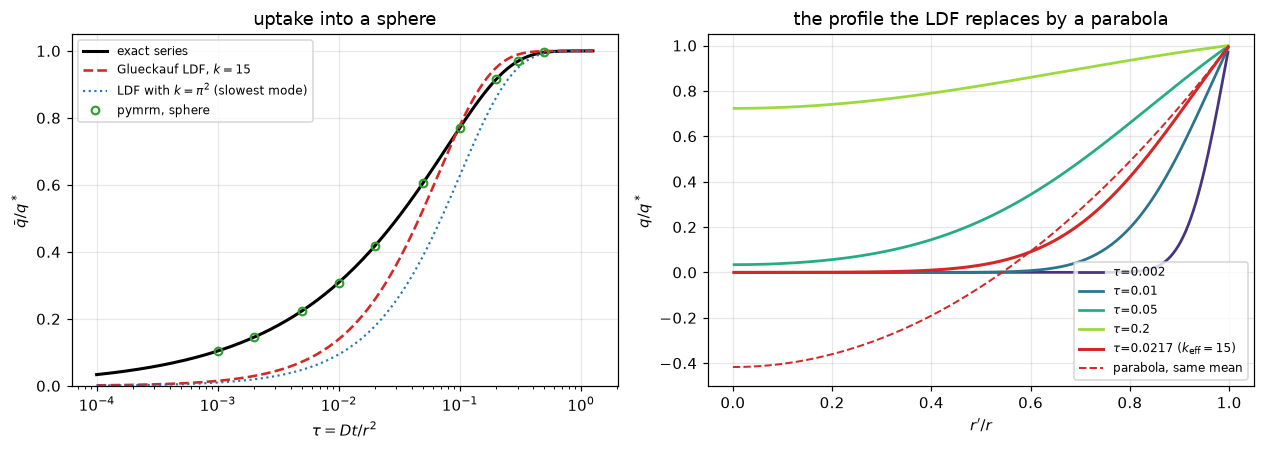
What “15 is exact at one instant” means. The coefficient the LDF would need, \(k_{\mathrm{eff}} = (\mathrm{d}\bar q/\mathrm{d}\tau)/(1 - \bar q)\), equals 15 when the surface gradient equals that of the parabola with the same mean. It does not mean the profile is parabolic: at that instant, \(\tau = 0.0217\) with the particle 43 % loaded, the parabola that carries the particle’s mean runs to a centre loading of \(-0.42\), while the real centre is still empty (largest gap 0.417, printed above). The scan below measures the gap between the profile and the parabola of the same mean, in units of the unfilled fraction \(1-\bar q\), at every time: the LDF’s assumption is closest to true in the middle of the uptake, where \(k_{\mathrm{eff}}\) is well below 15, and is no better met late in the uptake than at the instant of 15, because the profile settles into the first mode, not into a parabola.
ts = np.logspace(-3, 0, 121)
n_ts = crank_series(ts[0])["n_terms"]
q_ts = crank_uptake(ts, n_terms=n_ts)
# gap between the profile and the same-mean parabola, in units of the deficit 1 - qbar
dev_ts = np.array([np.max(np.abs(crank_profile(rho, t, n_ts)
                                 - (1.0 - 2.5 * (1.0 - q) * (1.0 - rho**2)))) / (1.0 - q)
                   for t, q in zip(ts, q_ts)])
i_min = int(np.argmin(dev_ts))
print("largest gap between the profile and the parabola with the same mean, over 1 - qbar:")
for t in (0.001, TAU15, 0.1, 1.0):
    j = int(np.argmin(np.abs(ts - t)))
    print(f"   tau = {ts[j]:.4f}   uptake {q_ts[j] * 100:5.1f} %   gap / (1 - qbar) {dev_ts[j]:.3f}")
print(f"on this scan the closest approach is at tau = {ts[i_min]:.3f} "
      f"(uptake {q_ts[i_min] * 100:.0f} %), gap / (1 - qbar) = {dev_ts[i_min]:.3f}, "
      f"where k_eff = {k_effective(ts[i_min], n_terms=n_ts)[0]:.1f}")
largest gap between the profile and the parabola with the same mean, over 1 - qbar:
tau = 0.0010 uptake 10.4 % gap / (1 - qbar) 1.384
tau = 0.0211 uptake 42.9 % gap / (1 - qbar) 0.750
tau = 0.1000 uptake 77.0 % gap / (1 - qbar) 0.581
tau = 1.0000 uptake 100.0 % gap / (1 - qbar) 0.790
on this scan the closest approach is at tau = 0.050 (uptake 61 %), gap / (1 - qbar) = 0.090, where k_eff = 11.6# The LDF error: its two extrema (zeros of its derivative) and its one crossing.
(t_lo, t_hi), (err_lo, err_hi) = ldf_error_extremes(15.0)
T_CROSS = ldf_crossing(15.0)
n_early = crank_series(1e-4)["n_terms"]
EARLY = float(1.0 - ldf_uptake(1e-4) / crank_uptake(1e-4, n_terms=n_early)[0])
print(f"under-prediction: largest {abs(err_lo):.4f} in qbar/q* at tau = {t_lo:.4f}")
print(f"the LDF crosses the exact curve at tau = {T_CROSS:.4f}")
print(f"over-prediction: largest {err_hi:.4f} at tau = {t_hi:.4f}")
print(f"at tau = 1e-4 the LDF is {EARLY * 100:.1f} % below the exact uptake, and the shortfall "
"tends to 100 % as tau -> 0 (15 tau against 6 sqrt(tau/pi))")
claims.value("ldf_worst_abs_err", abs(err_lo), unit="-")
claims.value("ldf_worst_abs_err_tau", t_lo, unit="-")
claims.value("ldf_crossing_tau", T_CROSS, unit="-")
claims.value("ldf_over_prediction_tau", t_hi, unit="-")
claims.value("ldf_over_prediction_max", err_hi, unit="-")
claims.value("ldf_max_rel_err_early", EARLY, unit="-",
note="relative shortfall at tau = 1e-4, the smallest tau of the scan")
claims.value("k_eff_equals_15_tau", TAU15, unit="-")
claims.value("uptake_at_k_eff_15", Q15, unit="-")
claims.value("profile_gap_at_k_eff_15", DEV15, unit="-")
_w = ldf_error_extremes(12.0)
_t12 = k_effective_crossing(12.0)
_n12 = crank_series(_t12)["n_terms"]
_q12 = float(crank_uptake(_t12)[0])
_dev12 = float(np.max(np.abs(crank_profile(rho, _t12, _n12) - (1.0 - 2.5 * (1.0 - _q12) * (1.0 - rho**2)))))
brk("LDF constant 12 instead of 15", "ldf_worst_abs_err", abs(_w[1][0]))
brk("LDF constant 12 instead of 15", "ldf_worst_abs_err_tau", _w[0][0])
brk("LDF constant 12 instead of 15", "ldf_over_prediction_max", _w[1][1])
brk("LDF constant 12 instead of 15", "ldf_crossing_tau", ldf_crossing(12.0))
brk("LDF constant 12 instead of 15", "ldf_over_prediction_tau", _w[0][1])
brk("LDF constant 60 instead of 15", "ldf_max_rel_err_early",
float(1.0 - ldf_uptake(1e-4, 60.0) / crank_uptake(1e-4, n_terms=n_early)[0]))
brk("coefficient 12 instead of 15 (k_effective_crossing(12))", "k_eff_equals_15_tau", _t12)
brk("coefficient 12 instead of 15 (k_effective_crossing(12))", "uptake_at_k_eff_15", _q12)
brk("coefficient 12 instead of 15 (k_effective_crossing(12))", "profile_gap_at_k_eff_15", _dev12)under-prediction: largest 0.1701 in qbar/q* at tau = 0.0118
the LDF crosses the exact curve at tau = 0.0940
over-prediction: largest 0.0358 at tau = 0.1776
at tau = 1e-4 the LDF is 95.5 % below the exact uptake, and the shortfall tends to 100 % as tau -> 0 (15 tau against 6 sqrt(tau/pi))So the LDF with Glueckauf’s 15 under-predicts uptake from an empty particle by at most \(0.170\) (in \(\bar q/q^*\)) at \(\tau = 0.0118\), crosses the exact curve at \(\tau = 0.094\), and over-predicts by at most \(0.036\) at \(\tau = 0.178\). At \(\tau = 0.0217\) (the instant at which 15 is the coefficient it would need) the particle is already 43 % loaded, and at \(\tau = 10^{-4}\) the LDF is 96 % below the exact uptake, a shortfall that tends to 100 % as \(\tau \to 0\), because 15\(\tau\) cannot follow \(6\sqrt{\tau/\pi}\).
The coefficient the LDF would need, instant by instant
Glueckauf argued from tabulated comparisons at a handful of points. With the exact solution in closed form the question can be put directly: at each instant, what coefficient would the LDF have to use to be right?
\[ k_{\mathrm{eff}}(\tau) = \frac{\mathrm{d}\bar q/\mathrm{d}\tau}{q^{*}-\bar q} \]
If any single constant were correct, this would be flat. Both the deficit and its rate come straight from the series, so nothing is differentiated numerically and nothing is formed as \(1 - (1 - \varepsilon)\), which loses all precision once the particle is nearly full. At short times a thin shell is penetrated, \(\bar q \approx 6\sqrt{\tau/\pi}\), so \(k_{\mathrm{eff}} \to 3/\sqrt{\pi\tau}\); at long times the first mode dominates, \(k_{\mathrm{eff}} = \pi^2\,[1 + \tfrac34 \mathrm{e}^{-3\pi^2\tau} + \dots]\).
tau_k = np.logspace(-4, 0.6, 400)
k_eff = k_effective(tau_k, n_terms=n_fine)
fig, ax = plt.subplots(figsize=(7.4, 4.4))
ax.loglog(tau_k, k_eff, color="tab:blue", lw=2.0, label=r"$k_{\mathrm{eff}}(\tau)$, exact")
ax.axhline(15.0, color="tab:red", lw=1.5, ls="--", label="Glueckauf 15 (parabolic profile)")
ax.axhline(np.pi**2, color="tab:green", lw=1.5, ls=":", label=r"$\pi^2$ = 9.87 (slowest eigenmode)")
early = tau_k < 3e-3
ax.loglog(tau_k[early], 3.0 / np.sqrt(np.pi * tau_k[early]), color="k", lw=1.1, ls="-.",
          label=r"thin shell, $3/\sqrt{\pi\tau}$")
ax.plot([TAU15], [15.0], "o", color="tab:red")
ax.set(xlabel=r"$\tau = Dt/r^2$", ylabel=r"$k_{\mathrm{eff}}\,r^2/D$", ylim=(5, 300),
       title="the coefficient the LDF would need, instant by instant")
ax.legend(fontsize=8)
fig.tight_layout()
plt.show()

T_THIN = 1e-6
n_thin = crank_series(T_THIN)["n_terms"]
THIN = float(k_effective(T_THIN, n_terms=n_thin)[0] * np.sqrt(np.pi * T_THIN) / 3.0)
T_LATE = 0.5
K_LATE = float(k_effective(T_LATE)[0])
GAP_LATE = K_LATE / np.pi**2 - 1.0
print(f"thin shell: k_eff sqrt(pi tau)/3 = {THIN:.4f} at tau = {T_THIN:g} ({n_thin} terms)")
print(f"late: k_eff(tau = {T_LATE}) = {K_LATE:.7f}, pi^2 = {np.pi**2:.7f}; "
      f"k_eff/pi^2 - 1 = {GAP_LATE:.3e} against the first correction "
      f"3/4 exp(-3 pi^2 tau) = {0.75 * np.exp(-3 * np.pi**2 * T_LATE):.3e}")
print(f"below tau = 1e-3 it exceeds {k_effective(1e-3)[0]:.0f} and is still climbing")
claims.bound("k_eff_thin_shell_ratio", THIN, min=1.0, max=1.01, basis="theory",
             note="k_eff sqrt(pi tau)/3 tends to 1 from above (qbar ~ 6 sqrt(tau/pi))")
claims.value("k_eff_gap_pi2", GAP_LATE, unit="-")
claims.value("long_time_decay_constant", K_LATE, rtol=1e-3, unit="-")
_n3 = 3
brk("series cut at three terms", "k_eff_thin_shell_ratio",
    float(k_effective(T_THIN, n_terms=_n3, rtol=np.inf)[0] * np.sqrt(np.pi * T_THIN) / 3.0))
brk("series cut at one term (only the slowest mode)", "k_eff_gap_pi2",
    float(k_effective(T_LATE, n_terms=1, rtol=np.inf)[0] / np.pi**2 - 1.0))
brk("decay constant read early, at tau = 0.05", "long_time_decay_constant",
    float(k_effective(0.05)[0]))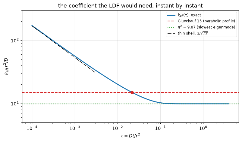
thin shell: k_eff sqrt(pi tau)/3 = 1.0016 at tau = 1e-06 (1807 terms)
late: k_eff(tau = 0.5) = 9.8696072, pi^2 = 9.8696044; k_eff/pi^2 - 1 = 2.790e-07 against the first correction 3/4 exp(-3 pi^2 tau) = 2.790e-07
below tau = 1e-3 it exceeds 56 and is still climbing
So Glueckauf’s 15 is the coefficient the particle needs at one instant, \(\tau = 0.0217\) with the particle 43 % loaded, and there it is a statement about the surface gradient, not about the profile. Before it the true coefficient is climbing without bound like \(3/\sqrt{\pi\tau}\), and after it the coefficient settles towards \(\pi^2 = 9.87\), which it reaches to within about \(3\times10^{-7}\) (relative) by \(\tau = 0.5\).
That is why the paper’s own conclusion is framed the way it is. Near equilibrium, with a linear or mildly curved isotherm, a particle never sees a step: it stays close to its surface value and lives in the region where 15 is a good constant, and the LDF is, in his words, fully adequate. Give it a steep front (a fresh particle meeting a step, his \(K_d > 3\) case) and the process happens entirely in the region the LDF cannot represent, where it under-predicts uptake by tens of percent.
Nothing here overturns the 15. It shows what the number is for, which is harder to see from the paper than it should be given how far the constant has travelled since, usually without its caveats.
Validation
Five checks: the reference series against itself and against the discretisation, the discretisation against its own refinement in space and in time, a flux balance, and the geometry argument. The break table at the end of the section lists every defect injected and what it did.
1. The series, summed to a measured tail bound
The terms \(t_n = \mathrm{e}^{-n^2\pi^2\tau}/n^2\) have ratios \(t_{m+1}/t_m\) that decrease with \(m\), so the tail after \(N\) terms is at most \(t_{N+1}/(1 - t_{N+2}/t_{N+1})\). The number of terms is the smallest for which that bound, relative to each sum, is below \(10^{-15}\) at the smallest \(\tau\) asked for. The independent check that the series itself is right is the discretised problem: solved exact in time (an eigendecomposition of the same operator, so the only error left is spatial) and extrapolated in \(n_r\).
for t in (1e-6, 1e-4, 1e-3, 0.5, 4.0):
    s = crank_series(t)
    print(f"tau = {t:<7g} {s['n_terms']:5d} terms, relative tail bound below 1e-15 (here {s['tail']:.1e})")
TAIL = max(crank_series(TAUS)["tail"], crank_series(1e-4)["tail"], crank_series(1e-6)["tail"])
claims.bound("series_tail_bound", TAIL, max=1e-15, basis="tolerance",
             note="relative tail bound of both sums at the requested rtol 1e-15")
brk("series cut at 20 terms", "series_tail_bound", float(crank_tail(TAUS, 20).max()))

NS_X = (100, 200, 400, 800)
SP = {n: Particle(n).exact_in_time(TAUS)["mean"] for n in NS_X}
OBS_X = [observed_orders(lambda n, j=j: SP[n][j], NS_X) for j in range(len(TAUS))]
LIMIT = np.array([o["extrapolated"] for o in OBS_X])
GAP_SERIES = float(np.max(np.abs(LIMIT / EX - 1.0)))
print(f"\nspatial limit of the discretisation (exact in time, extrapolated in n_r) against the series:"
      f"\n   worst relative gap over the ten times: below 1e-6 (here {GAP_SERIES:.1e})")
claims.bound("series_vs_pymrm_limit", GAP_SERIES, max=1e-6, basis="chosen",
             note="Richardson-extrapolated spatial limit against the series, ten times; "
                  "set an order of magnitude above the measured gap")
_bad = [observed_orders(lambda n, j=j: Particle(n, nu_div=1).exact_in_time(TAUS)["mean"][j],
                        (100, 200, 400))["extrapolated"] for j in range(len(TAUS))]
brk("geometry index 1 in construct_div for a sphere (nu_div=1)", "series_vs_pymrm_limit",
    float(np.max(np.abs(np.array(_bad) / EX - 1.0))))
tau = 1e-06 1807 terms, relative tail bound below 1e-15 (here 9.9e-16)
tau = 0.0001 181 terms, relative tail bound below 1e-15 (here 7.6e-16)
tau = 0.001 57 terms, relative tail bound below 1e-15 (here 6.6e-16)
tau = 0.5 2 terms, relative tail bound below 1e-15 (here 7.2e-18)
tau = 4 1 terms, relative tail bound below 1e-15 (here 3.7e-52)
spatial limit of the discretisation (exact in time, extrapolated in n_r) against the series:
worst relative gap over the ten times: below 1e-6 (here 2.0e-07)2. Refinement in space
The solution of the discretised problem is compared with itself on nested grids (pymrm.checks.observed_orders), which needs no reference, and the time is taken exact (the eigendecomposition route) so that the step does not enter. Every one of the ten times is checked separately. The finest difference must also be well above the round-off floor of the eigen route, \(\mathrm{cond}(V)\,\varepsilon\) with \(V\) the eigenvector matrix, or the order is fitted to noise.
print("   tau     orders (100,200,400,800)      finest triple")
ORD_X = []
for j, t in enumerate(TAUS):
    o = OBS_X[j]["orders"]
    ORD_X.append(o[-1])
    print(f"{t:>7.3f}   " + "  ".join(f"{x:5.3f}" for x in o) + f"      {o[-1]:5.3f}")
DEV_X = float(np.max(np.abs(np.array(ORD_X) - 2.0)))
COND_V = float(np.linalg.cond(Particle(800).spectrum()[1]))
FIN_X = float(np.min([abs(SP[800][j] - SP[400][j]) / SP[800][j] for j in range(len(TAUS))]) / (COND_V * EPS))
print(f"\nworst departure of the finest-triple order from 2: {DEV_X:.3f}, below 0.2")
print(f"smallest finest relative difference over round-off floor cond(V) eps (cond(V) = {COND_V:.0f}): above 1e3 (here {FIN_X:.1e})")
claims.bound("grid_order_worst_dev", DEV_X, max=0.2, basis="theory",
             note="|observed order - 2| at the finest triple, worst of ten times, midpoint "
                  "scheme with a Dirichlet face value")
claims.bound("grid_finest_over_roundoff", FIN_X, min=1e3, basis="theory",
             note="finest relative difference over cond(V) eps, smallest of ten times")
_m300 = Particle(300).exact_in_time(TAUS)["mean"]
_bad_ord = [order_of(SP[100][j], SP[200][j], _m300[j]) for j in range(len(TAUS))]
brk("ladder 100, 200, 300 read as a ratio of 2", "grid_order_worst_dev",
    float(np.max(np.abs(np.array(_bad_ord) - 2.0))))
_g4 = {n: Particle(n).exact_in_time([4.0])["mean"][0] for n in (400, 800)}
# the difference is zero or one ulp depending on the kernel: floor it at one ulp
brk("ladders read at tau = 4, mean 1 to round-off", "grid_finest_over_roundoff",
    max(abs(_g4[800] - _g4[400]), EPS) / _g4[800] / (COND_V * EPS))
tau orders (100,200,400,800) finest triple
0.001 1.945 1.909 1.909
0.002 1.873 1.919 1.919
0.005 1.897 1.946 1.946
0.010 1.928 1.964 1.964
0.020 1.954 1.977 1.977
0.050 1.977 1.988 1.988
0.100 1.987 1.993 1.993
0.200 1.992 1.996 1.996
0.300 1.993 1.997 1.997
0.500 1.995 1.997 1.997
worst departure of the finest-triple order from 2: 0.091, below 0.2
smallest finest relative difference over round-off floor cond(V) eps (cond(V) = 1351): above 1e3 (here 3.2e+05)3. Refinement in time
At fixed \(n_r = 200\) the backward-Euler march is refined from 10 to 80 steps per \(10^{-3}\) of \(\tau\) (the production step is 50), again by successive differences. The semi-discrete value (exact in time) is the limit the ladder should approach, so the share of the total error that is the step follows.
NS_T = (10, 20, 40, 80)
TM = {m: p.march(TAUS, 1e-3 / m)["mean"] for m in NS_T}
OBS_T = [observed_orders(lambda m, j=j: TM[m][j], NS_T) for j in range(len(TAUS))]
print("   tau     orders (10,20,40,80)       finest")
for j, t in enumerate(TAUS):
    o = OBS_T[j]
    print(f"{t:>7.3f}   " + "  ".join(f"{x:5.3f}" for x in o["orders"]) + f"      {o['orders'][-1]:5.3f}")
EXTRAP = max(abs(o["extrapolated"] / SP[200][j] - 1) for j, o in enumerate(OBS_T))
print(f"\nthe ladder's Richardson limit against the value exact in time: below 1e-5 (here {EXTRAP:.1e})")
DEV_T = float(max(abs(o["orders"][-1] - 1.0) for o in OBS_T))
FIN_T = float(np.min([abs(TM[80][j] - TM[40][j]) / TM[80][j] for j in range(len(TAUS))])
              / (int(0.5 / (1e-3 / 80)) * EPS))
print(f"\nworst departure of the finest-triple order from 1 (backward Euler): below 0.1 (here {DEV_T:.3f})")
print(f"smallest finest relative difference over round-off floor (n_steps eps): above 1e3 (here {FIN_T:.1e})")
claims.bound("time_order_worst_dev", DEV_T, max=0.1, basis="theory",
             note="|observed order - 1| at the finest triple, backward Euler, worst of ten times")
claims.bound("dt_finest_over_roundoff", FIN_T, min=1e3, basis="theory",
             note="finest relative difference over n_steps eps, smallest of ten times")
_tm30 = p.march(TAUS, 1e-3 / 30)["mean"]
_bad_t = [order_of(TM[10][j], TM[20][j], _tm30[j]) for j in range(len(TAUS))]
brk("ladder 10, 20, 30 read as a ratio of 2", "time_order_worst_dev",
    float(max(abs(o - 1.0) for o in _bad_t)))
_t4 = {m: p.march([4.0], 1e-3 / m)["mean"][0] for m in (40, 80)}
brk("ladders read at tau = 4, mean 1 to round-off", "dt_finest_over_roundoff",
    max(abs(_t4[80] - _t4[40]), EPS) / _t4[80] / (int(0.5 / (1e-3 / 80)) * EPS))

# Where the production error comes from, at the worst time.
J0 = 0
tot, spa = abs(PROD["mean"][J0] / EX[J0] - 1), abs(SP[200][J0] / EX[J0] - 1)
SHARE = abs(PROD["mean"][J0] / SP[200][J0] - 1) / tot
print(f"\nat tau = {TAUS[J0]}: total error {tot:.2e}, spatial part {spa:.2e}, "
      f"the step is {SHARE * 100:.0f} % of it")
claims.value("time_error_share_tau1e3", SHARE, unit="-")
claims.value("spatial_err_tau1e3", spa, unit="-")
brk("25 cells instead of 200 (spatial error comparable to the step's)", "time_error_share_tau1e3",
    abs(Particle(25).march(TAUS[:1], DT)["mean"][0] / Particle(25).exact_in_time(TAUS[:1])["mean"][0] - 1)
    / abs(Particle(25).march(TAUS[:1], DT)["mean"][0] / EX[0] - 1))
brk("25 cells instead of 200 (spatial error comparable to the step's)", "spatial_err_tau1e3",
    abs(Particle(25).exact_in_time(TAUS[:1])["mean"][0] / EX[0] - 1))

print("\n   n_r    rel err vs the series at tau = 0.05 (production step)   ratio")
_prev = None
for n in (25, 50, 100, 200, 400):
    _e = abs(Particle(n).march(TAUS[5:6], DT)["mean"][0] / EX[5] - 1)
    print(f"{n:>5}    {_e:.2e}" + ("" if _prev is None else f"{_prev / _e:>52.2f}"))
    _prev = _e

WORST = float(rel.max())
N400 = float(abs(Particle(400).march(TAUS[5:6], DT)["mean"][0] / EX[5] - 1))
print(f"\nproduction march (n_r = {N_R}, dt = {DT:g}) against the series: worst {WORST:.2e} "
      f"at tau = {TAUS[int(rel.argmax())]}; at tau = 0.05 on 400 cells: {N400:.2e}")
claims.value("solver_worst_rel_err", WORST, unit="-")
claims.value("solver_rel_err_n400", N400, unit="-")
_bd = Particle(N_R, nu_div=1).march(TAUS, DT)["mean"]
brk("geometry index 1 in construct_div for a sphere (nu_div=1)", "solver_worst_rel_err",
    float(np.max(np.abs(_bd / EX - 1.0))))
brk("geometry index 1 in construct_div for a sphere (nu_div=1)", "solver_rel_err_n400",
    float(abs(Particle(400, nu_div=1).march(TAUS[5:6], DT)["mean"][0] / EX[5] - 1)))
tau orders (10,20,40,80) finest
0.001 0.992 0.996 0.996
0.002 0.996 0.998 0.998
0.005 0.999 0.999 0.999
0.010 0.999 1.000 1.000
0.020 1.000 1.000 1.000
0.050 1.000 1.000 1.000
0.100 1.000 1.000 1.000
0.200 1.000 1.000 1.000
0.300 1.000 1.000 1.000
0.500 1.001 1.000 1.000
the ladder's Richardson limit against the value exact in time: below 1e-5 (here 5.4e-06)
worst departure of the finest-triple order from 1 (backward Euler): below 0.1 (here 0.004)
smallest finest relative difference over round-off floor (n_steps eps): above 1e3 (here 1.5e+05)
at tau = 0.001: total error 2.64e-03, spatial part 7.54e-05, the step is 97 % of it
n_r rel err vs the series at tau = 0.05 (production step) ratio
25 6.79e-04
50 2.25e-04 3.01
100 1.04e-04 2.16
200 7.30e-05 1.43
400 6.50e-05 1.12
production march (n_r = 200, dt = 2e-05) against the series: worst 2.64e-03 at tau = 0.001; at tau = 0.05 on 400 cells: 6.50e-05Refining \(n_r\) alone against the series stalls, because the backward-Euler step then dominates; at the worst time, 97 % of the error is the step. That is a property of the step, not of the grid, and the two ladders above separate them. The table shows the stall at \(\tau = 0.05\) (production step).
4. A flux balance
Because the weights are the cell volumes and the divergence is conservative, the increase of the mean over a step is exactly \((\nu+1)\,\Delta\tau\) times the surface flux that step: the mean-loading equation is the integral of the flux the operators transported. It holds for any backward-Euler step, so it checks the weights, the geometry index and the flux reading, not the physics.
def balance_gap(pt, tau_end=0.05, dt=DT):
    """Largest gap between the mean and the time integral of the surface flux."""
    res = pt.march(np.array([tau_end]), dt, keep=True)
    means = pt.mean(res["states"])
    cum = (pt.nu + 1) * dt * np.cumsum(pt.surface_flux(res["states"]))
    return float(np.max(np.abs(means - cum)))


BAL = balance_gap(p)
print(f"max |mean(tau) - (nu+1) integral of the surface flux| over 2500 steps: below 1e-12 (here {BAL:.1e})")
claims.bound("flux_balance_gap", BAL, max=1e-12, basis="identity",
             note="exact for backward Euler with cell-volume weights and the face flux")
brk("midpoint weights (Particle(weights='midpoint'))", "flux_balance_gap",
    balance_gap(Particle(N_R, weights="midpoint")))
brk("geometry index 1 in construct_div (nu_div=1)", "flux_balance_gap",
    balance_gap(Particle(N_R, nu_div=1)))
brk("flux from the last cell centre (Particle(flux_from='cell'))", "flux_balance_gap",
    balance_gap(Particle(N_R, flux_from="cell")))
max |mean(tau) - (nu+1) integral of the surface flux| over 2500 steps: below 1e-12 (here 1.9e-15)5. The geometry argument and the other particle shapes
The same class with nu=1 or nu=0 is a long cylinder or a slab. Their slowest mode decays at \(j_{0,1}^2 = 5.783\) and \((\pi/2)^2 = 2.467\) (the sphere’s is \(\pi^2\)), and the discrete operator’s lowest eigenvalue reproduces each at the second order of the scheme. The parabolic-profile constants follow from the argument in The published model, \((\nu+1)(\nu+3)\).
LAM_EXACT = {2: np.pi**2, 1: float(jn_zeros(0, 1)[0] ** 2), 0: (np.pi / 2) ** 2}
LAM_ERR = {}
print(f"{'nu':>3}{'shape':>10}{'lowest eigenvalue':>20}{'exact':>10}{'rel err':>11}{'parabolic constant':>20}")
for nu, name in ((2, "sphere"), (1, "cylinder"), (0, "slab")):
    lam1 = Particle(N_R, nu=nu).spectrum()[0][0]
    LAM_ERR[nu] = abs(lam1 / LAM_EXACT[nu] - 1)
    print(f"{nu:>3}{name:>10}{lam1:>20.5f}{LAM_EXACT[nu]:>10.5f}{LAM_ERR[nu]:>11.1e}{ldf_constant(nu):>20.0f}")
claims.value("lambda1_worst_rel_err", max(LAM_ERR.values()), unit="-")
claims.exact("ldf_constant_sphere", ldf_constant(2), note="(nu + 1)(nu + 3) at nu = 2")
claims.exact("ldf_constant_cylinder", ldf_constant(1))
claims.exact("ldf_constant_slab", ldf_constant(0))
for nu, name in ((2, "sphere"), (1, "cylinder"), (0, "slab")):
    _wrong = nu + 1 if nu < 2 else 1
    brk(f"geometry index {_wrong} in construct_div for the {name}", "lambda1_worst_rel_err",
        max(abs(Particle(N_R, nu=nu, nu_div=_wrong).spectrum()[0][0] / LAM_EXACT[nu] - 1),
            0.0))
    brk(f"parabola of geometry {_wrong} for the {name}", f"ldf_constant_{name}", ldf_constant(_wrong))
nu shape lowest eigenvalue exact rel err parabolic constant
2 sphere 9.86936 9.86960 2.5e-05 15
1 cylinder 5.78310 5.78319 1.4e-05 8
0 slab 2.46739 2.46740 5.1e-06 3The break table
print(f"{'injected defect':<66} {'claim':<28} {'clean':>11} {'broken':>11}  caught")
for row, metric, clean, broken, caught in BREAK:
    if claims.metrics[metric]["kind"] == "bound":
        shown, br = f"(here {clean:.3g})", f"{float(broken):.3g}"
    else:
        shown, br = f"{float(clean):11.5g}", f"{float(broken):11.5g}"
    print(f"{row[:66]:<66} {metric[:28]:<28} {shown:>11} {br:>11}  {'yes' if caught else 'NO'}")
_caught = {mt for _, mt, _, _, c in BREAK if c}
_open = sorted(k for k in claims.metrics if k not in _caught and not claims.metrics[k].get("structural"))
print(f"\n{len(BREAK)} rows; {len(_caught)} of {len(claims.metrics)} claims are failed by at least one row; "
      f"open: {', '.join(_open) or 'none'}")
print("rows that do not fail their claim: "
      + ("; ".join(f"{r} -> {mt}" for r, mt, _, _, c in BREAK if not c) or "none"))
injected defect claim clean broken caught
midpoint weights 3 r_c^2 dr (Particle(weights='midpoint')) weights_sum_gap (here 0) 6.25e-06 yes
LDF constant 12 instead of 15 ldf_worst_abs_err 0.1701 0.20591 yes
LDF constant 12 instead of 15 ldf_worst_abs_err_tau 0.011831 0.017776 yes
LDF constant 12 instead of 15 ldf_over_prediction_max 0.03581 0.0043508 yes
LDF constant 12 instead of 15 ldf_crossing_tau 0.094008 0.2335 yes
LDF constant 12 instead of 15 ldf_over_prediction_tau 0.17759 0.32533 yes
LDF constant 60 instead of 15 ldf_max_rel_err_early 0.95533 0.82171 yes
coefficient 12 instead of 15 (k_effective_crossing(12)) k_eff_equals_15_tau 0.021652 0.044192 yes
coefficient 12 instead of 15 (k_effective_crossing(12)) uptake_at_k_eff_15 0.43315 0.57904 yes
coefficient 12 instead of 15 (k_effective_crossing(12)) profile_gap_at_k_eff_15 0.4172 0.071142 yes
series cut at three terms k_eff_thin_shell_ratio (here 1) 0.0129 yes
series cut at one term (only the slowest mode) k_eff_gap_pi2 2.7899e-07 0 yes
decay constant read early, at tau = 0.05 long_time_decay_constant 9.8696 11.625 yes
series cut at 20 terms series_tail_bound (here 9.86e-16) 0.00444 yes
geometry index 1 in construct_div for a sphere (nu_div=1) series_vs_pymrm_limit (here 1.99e-07) 0.1 yes
ladder 100, 200, 300 read as a ratio of 2 grid_order_worst_dev (here 0.0908) 0.428 yes
ladders read at tau = 4, mean 1 to round-off grid_finest_over_roundoff (here 3.23e+05) 0.00074 yes
ladder 10, 20, 30 read as a ratio of 2 time_order_worst_dev (here 0.00357) 0.586 yes
ladders read at tau = 4, mean 1 to round-off dt_finest_over_roundoff (here 1.51e+05) 0.0774 yes
25 cells instead of 200 (spatial error comparable to the step's) time_error_share_tau1e3 0.97156 0.14213 yes
25 cells instead of 200 (spatial error comparable to the step's) spatial_err_tau1e3 7.5407e-05 0.023485 yes
geometry index 1 in construct_div for a sphere (nu_div=1) solver_worst_rel_err 0.0026443 0.10048 yes
geometry index 1 in construct_div for a sphere (nu_div=1) solver_rel_err_n400 6.5028e-05 0.083941 yes
midpoint weights (Particle(weights='midpoint')) flux_balance_gap (here 1.89e-15) 2.12e-06 yes
geometry index 1 in construct_div (nu_div=1) flux_balance_gap (here 1.89e-15) 0.122 yes
flux from the last cell centre (Particle(flux_from='cell')) flux_balance_gap (here 1.89e-15) 0.00336 yes
geometry index 1 in construct_div for the sphere lambda1_worst_rel_err 2.4667e-05 0.41405 yes
parabola of geometry 1 for the sphere ldf_constant_sphere 15 8 yes
geometry index 2 in construct_div for the cylinder lambda1_worst_rel_err 2.4667e-05 0.70656 yes
parabola of geometry 2 for the cylinder ldf_constant_cylinder 8 15 yes
geometry index 1 in construct_div for the slab lambda1_worst_rel_err 2.4667e-05 1.3438 yes
parabola of geometry 1 for the slab ldf_constant_slab 3 8 yes
32 rows; 28 of 28 claims are failed by at least one row; open: none
rows that do not fail their claim: noneWhat pymrm adds
Nothing to the answer. Everything this page concludes about the LDF (where 15 is exact, how it fails, the thin-shell and slowest-mode limits) comes from the closed-form series, which uses no pymrm; even the profiles have a series.
What the pymrm solve is for. It is the inner problem of a coupled column, which has no closed form once the isotherm is nonlinear or the diffusivity varies: when the surface value tracks a bulk the particle is depleting, the LDF is the usual shortcut and the sphere has to be solved. This page shows that the discretisation of that inner problem is consistent, with its measured errors: second order in space (within 0.2 of 2 at every tabulated time), first order in time, an exact flux balance, and a geometry index (nu) that is a one-argument change. It also shows the cost of the plain backward-Euler step: at \(\tau = 0.001\) it is 97 % of the error. The operators, the boundary conditions with their outward normal, the face-value flux and the checks (observed_orders, find_roots) are pymrm’s; the coupled column itself is not solved here.
Reuse
The particle is the reusable part. Particle is a bare transient diffusion solve; nu=1 is a cylinder and nu=0 a slab, with parabolic-profile constants 8 and 3 and slowest-mode constants 5.783 and 2.467 (Validation 5).
Coupling it to a column. In a real breakthrough calculation the surface value \(q^*\) is not fixed: it tracks a bulk concentration that the particle is itself depleting. That is the S8 nested coupling: replace the Dirichlet surface condition with a flux matched to the bed equation, exactly as D1.4 does for a catalyst pellet. This page is the inner problem of that pair, and the LDF is what lets it be skipped. The constant operators stay as they are; only the surface boundary value becomes an external unknown (shapes_d in construct_grad).
When you can use the shortcut. Near-equilibrium operation with a linear or mildly curved isotherm: yes, and the error in fractional uptake stays small (the figures above are for the harshest case, a step from an empty particle). Steep fronts, nearly irreversible exchange, or anything where the particle sees a step: solve the sphere.
Related pages. B1.1 (the steady version of the same particle), D1.4 (the nested coupling), J1.1, J1.6.
Cite the source, not this page: Glueckauf, E., Theory of chromatography. Part 10. Formulae for diffusion into spheres and their application to chromatography, Trans. Faraday Soc. 51 1540-1551 (1955), doi:10.1039/TF9555101540
# Numbers stated in the Markdown cells, each checked against its claim.
PROSE = [("0.0217", "k_eff_equals_15_tau"), ("43 %", "uptake_at_k_eff_15"),
         ("0.417", "profile_gap_at_k_eff_15"), ("0.170", "ldf_worst_abs_err"),
         ("0.0118", "ldf_worst_abs_err_tau"), ("0.094", "ldf_crossing_tau"),
         ("0.036", "ldf_over_prediction_max"), ("0.178", "ldf_over_prediction_max"),
         ("96 %", "ldf_max_rel_err_early"), ("9.87", "long_time_decay_constant"),
         ("3e-7", "k_eff_gap_pi2"), ("0.42", "profile_gap_at_k_eff_15"),
         ("97 %", "time_error_share_tau1e3")]
PROSE = [(lit, name) if name != "ldf_over_prediction_max" or lit != "0.178"
         else (lit, "ldf_over_prediction_tau") for lit, name in PROSE]
for _lit, _name in PROSE:
    claims.says(_lit, _name)
print(f"{len(PROSE)} prose literals checked against {len({n for _, n in PROSE})} claims")
13 prose literals checked against 12 claims# Claims: prints every registered number, writes agreement.json for CI, and
# raises when a claim fails its own check or has no break row.
claims.report(); # the semicolon keeps the notebook from echoing the payloadClaims for J1.5:
weights_sum_gap = (here 0.0e+00) bound bound <= 1e-14 [identity]
ldf_worst_abs_err = 0.1701 value rtol 0.05
ldf_worst_abs_err_tau = 0.011831 value rtol 0.05
ldf_crossing_tau = 0.094008 value rtol 0.05
ldf_over_prediction_tau = 0.17759 value rtol 0.05
ldf_over_prediction_max = 0.03581 value rtol 0.05
ldf_max_rel_err_early = 0.95533 value rtol 0.05
k_eff_equals_15_tau = 0.021652 value rtol 0.05
uptake_at_k_eff_15 = 0.43315 value rtol 0.05
profile_gap_at_k_eff_15 = 0.4172 value rtol 0.05
k_eff_thin_shell_ratio = (here 1.0e+00) bound bound [1, 1.01] [theory]
k_eff_gap_pi2 = 2.7899e-07 value rtol 0.05
long_time_decay_constant = 9.8696 value rtol 0.001
series_tail_bound = (here 9.9e-16) bound bound <= 1e-15 [tolerance]
series_vs_pymrm_limit = (here 2.0e-07) bound bound <= 1e-06 [chosen]
grid_order_worst_dev = (here 9.1e-02) bound bound <= 0.2 [theory]
grid_finest_over_roundoff = (here 3.2e+05) bound bound >= 1000 [theory]
time_order_worst_dev = (here 3.6e-03) bound bound <= 0.1 [theory]
dt_finest_over_roundoff = (here 1.5e+05) bound bound >= 1000 [theory]
time_error_share_tau1e3 = 0.97156 value rtol 0.05
spatial_err_tau1e3 = 7.5407e-05 value rtol 0.05
solver_worst_rel_err = 0.0026443 value rtol 0.05
solver_rel_err_n400 = 6.5028e-05 value rtol 0.05
flux_balance_gap = (here 1.9e-15) bound bound <= 1e-12 [identity]
lambda1_worst_rel_err = 2.4667e-05 value rtol 0.05
ldf_constant_sphere = 15 exact exact
ldf_constant_cylinder = 8 exact exact
ldf_constant_slab = 3 exact exact