try:
    import pymrm
except ImportError:
%pip install -q pymrm pyyamlIAST 1965: mixture adsorption from pure-component isotherms alone — and a paper that prints no numbers
sec:J
struct:S1
struct:S10
tier:T0
data:tier6
phase:gas-solid
Myers and Prausnitz derive the ideal adsorbed solution theory — the Raoult’s-law analogue in which P y_i = P_i°(π) x_i at matched spreading pressure — and validate it on four gas pairs. Every one of those comparisons is a figure of external data, and even the pure-component inputs are never tabulated, so this page validates what the paper actually prints: the derivation chain (verified symbolically, which surfaces two printed equation defects), the graphical lever-rule construction, and the thermodynamic structure. The solver is proved against two closed forms it never touches — extended Langmuir, which the page derives symbolically as the exact IAST solution for equal capacities, and the Henry-law limit the paper itself proves rigorous. The inconsistency the paper reports for the Langmuir mixture rule is then made quantitative: integrating the Gibbs adsorption isotherm around a closed loop in (P, y) leaves a 12 % spreading-pressure mismatch for unequal-capacity extended Langmuir, where IAST closes the same loop to 8e-16 — computed twice, by line integral and by a symbolically derived curl.
IAST 1965: mixture adsorption from pure-component isotherms alone — and a paper that prints no numbers
Catalog ID: J1.4 · Structures: S1 (pointwise algebra), S10 (constrained algebraic system) · Tier: T0
The ideal adsorbed solution theory is the A2.1 of adsorption: the default mixture model everyone reaches for, sixty years on. Its content is one sentence — the paper’s own abstract sentence: the partial pressure of an adsorbed component is given by the product of its mole fraction in the adsorbed phase and the pressure which it would exert as a pure adsorbed component at the same temperature and spreading pressure as those of the mixture,
\[P y_i \;=\; P_i^{\circ}(\pi)\,x_i \qquad \text{(eq. 22)},\]
Raoult’s law with the pure-component reference taken at matched spreading pressure instead of matched temperature alone. Everything else follows from classical surface thermodynamics, and mixture equilibria follow from pure-component isotherms with no mixture data and no mixture parameters.
What this page can and cannot check, decided before any code. The paper validates IAST against four systems — methane–ethane and ethylene–carbon dioxide on activated carbon, carbon monoxide–oxygen and propane–propylene on silica gel. Every one of those comparisons is a figure (Figs. 3–10), the experimental points in them belong to four other papers, and even the pure-component isotherms that feed the theory are never tabulated — Fig. 2’s own legend box says its curves are calculated from the isotherms of Szepesy and Illés. There is not one table in the paper. So the experimental case is out of scope here (§4 gives the search and the reasoning), and the page validates what the paper actually prints:
- The derivation chain, symbolically. Eqs. (9)–(35) and (45)–(46) are re-derived with
sympy; eleven identities close to exactly zero. Doing this surfaces two printed equation defects: eq. (11) is missing the+between its two \(RT\ln\) terms — as printed it does not yield eq. (13), the equilibrium relation the whole theory rests on — and the sentence introducing eq. (21) cites eq. (21) itself where the derivation needs eq. (20). Both are reported, neither repaired silently. - The solver, against closed forms it never touches. The page derives symbolically that for two Langmuir isotherms of equal capacity the IAST solution is the extended Langmuir rule, and the numerical solver reproduces that closed form to 7.6e-16; in the Henry-law limit — the one case the paper itself proves IAST rigorous (eqs. 30–35) — the solver converges to the closed-form selectivity at first order in \(P\), as it must.
- The thermodynamic consistency the paper’s rivals lack, made quantitative. The paper reports (p. 125) that the Langmuir mixture model is “not thermodynamically consistent”. This page turns that sentence into a number: integrating the Gibbs adsorption isotherm (eq. 15) around a closed loop in \((P, y_1)\) leaves a spreading-pressure mismatch of 12 % of the loop’s own scale for extended Langmuir with unequal capacities — computed twice, by line integral and by a symbolically derived curl, two routes that agree to 2.7e-15 — while IAST closes the same loop to 7.8e-16. With equal capacities the curl is symbolically zero, which is exactly the case where extended Langmuir is an IAST.
- One structural result the paper stops short of. Under IAST, the selectivity coefficient is exactly constant whenever the two pure isotherms are the same curve shifted in \(\log P\) — the Henry limit of eqs. (30)–(35) is the linear special case — so the composition dependence the paper predicts in Fig. 10 is a measure of the two isotherms’ difference in shape, not in scale. Verified to 4.7e-14 on a dual-site pair the closed forms never see.
Nothing on this page is a fit — there is no data to fit — and nothing on it is experimental. This page establishes that the theory is what the paper says it is, not that it is empirically right. The empirical case lives in figures this page does not touch.
Background
The problem in 1965
Adsorption equilibria of gas mixtures are what separation design actually needs, and measuring them is far more work than measuring pure-component isotherms. The obvious programme — write the mixture isotherm’s parameters as functions of the pure-component parameters — had, in the paper’s words, “not been very successful; the predictions have not been in quantitative agreement with the experimental data (\(2\)) and often not even in qualitative agreement (\(1\))”. The one alternative on the table, Arnold’s liquid entropy model, the paper dismisses on two grounds it states plainly: “it is thermodynamically inconsistent and … separate numerical integrations are required for each vapor composition.”
Myers and Prausnitz instead import the machinery that had organised vapour–liquid equilibria for decades: treat the adsorbed phase as a solution, define activity coefficients for it, and let ideality be an empirical question. The move that makes this possible is recognising the spreading pressure \(\pi\) — the two-dimensional analogue of pressure, the intensive variable conjugate to adsorbent area \(A\) — as a full thermodynamic variable. There is “no experimental technique for measuring the spreading pressure directly”, the paper concedes, but it is computable from any measured isotherm through the Gibbs adsorption isotherm, and that is all the theory needs.
Three assumptions carry the thermodynamics (p. 121): the adsorbent is inert; it “possesses a temperature-invariant area which is the same for all adsorbates” — explicitly not valid for molecular sieves, where accessible area depends on the adsorbate; and adsorption is what the Gibbs definition says it is. On top of these the derivation assumes a perfect gas phase, which the paper defends for pressures “usually less than 1 atm.”
What the paper found, and why it was surprising
The original plan, the paper says, was to measure activity coefficients from mixture data and then interpret them. “Surprisingly, the calculated activity coefficients were found to be equal to unity within the experimental error” — so the ideal adsorbed solution, the \(\gamma_i = 1\) case, predicts the mixture equilibria outright, from pure-component isotherms alone. The conclusions call it “very surprising” a second time and are careful about why: the adsorbents in question are highly heterogeneous, no statistical model of them existed to compare against, and the paper explicitly declines to claim the result must generalise — mixtures of “highly dissimilar components … may show appreciable nonideality”.
Where this page’s siblings sit
The pure-component isotherms IAST consumes are the subject of J1.1 (Langmuir 1918) and J1.3 (BET 1938); either drops into this page’s \(F_i(P_i^{\circ})\) slot. Adsorption dynamics — breakthrough, the linear-driving-force law — is J1.5, and an IAST equilibrium can serve as that page’s mixture isotherm. This page is equilibrium only.
The published model
All equation numbers are the paper’s, read from a 300 ppi native render.
Thermodynamics of the adsorbed phase (eqs. 1–18)
Substituting \(-\pi\,dA\) for \(-P\,dV\) work makes the adsorbed phase a two-dimensional fluid:
\[dU = T\,dS - \pi\,dA + \Sigma \mu_i\,dn_i \tag{1}\] \[dG = -S\,dT + A\,d\pi + \Sigma \mu_i\,dn_i \tag{2}\]
so \(G = G(T, \pi, n_i)\) and, by Euler’s theorem, \(G = \Sigma n_i \mu_i\) (3). Activity coefficients are then defined exactly as for a liquid mixture, at constant \(T\) and \(\pi\) (5)–(8), giving the chemical potential
\[\mu_i(T,\pi,x_1\ldots) = g_i^{\circ}(T,\pi) + RT \ln \gamma_i x_i, \tag{9}\]
and, writing the pure-adsorbate reference through its equilibrium pressure \(P_i^{\circ}(\pi)\) at the same spreading pressure (10), then equating with the perfect-gas chemical potential (12), the equation of equilibrium for mixed-gas adsorption:
\[P y_i = P_i^{\circ}(\pi)\,\gamma_i x_i \quad (\text{constant } T). \tag{13}\]
Eq. (14) restates (13) with fugacities for high pressure. The Gibbs adsorption isotherm \(-A\,d\pi + \Sigma n_i\,d\mu_i = 0\) (15) yields the Gibbs–Duhem relation \(\Sigma x_i\,d\ln\gamma_i = 0\) at constant \(T\) and \(\pi\) (17), so the activity coefficients are thermodynamically consistent by construction — the failure the paper charges Arnold’s model with cannot occur here. The phase rule for adsorption (18) gives binary adsorption 3 degrees of freedom, one more than binary VLE, because area is an extra variable; the adsorbent itself is not counted (“The absorbent is not counted as a component in Equation (18) since it is assumed to be thermodynamically inert.” — sic, “absorbent”, p. 122; the paper spells “adsorbent” correctly everywhere else).
Two printed equation defects, reported and not repaired
Eq. (11) is missing its +. As printed (p. 122, verified on a crop of the 300 ppi native render):
\[\mu_i(T,\pi,x_1\ldots) = g_i^{\circ}(T) + RT \ln P_i^{\circ}(\pi)\;RT\ln\gamma_i x_i \qquad [sic] \tag{11}\]
— no operator between the two \(RT\ln\) terms. The product form is dimensionally incoherent (energy²) and §2.1 shows symbolically that equating it with eq. (12) does not produce eq. (13), while the sum form produces it exactly. Since (11) is by construction “Substituting Equation (10) into Equation (9)”, and both (10) and (9) are printed correctly, the defect is proved from the paper’s own equations; the repair (a lost +) is an inference, labelled as one.
The sentence introducing eq. (21) cites eq. (21). P. 123, verbatim: “With the pressure \(P\) of the mixture held constant, Equation (21) becomes” — and what follows is eq. (21). The derivation requires “Equation (20) becomes”: at constant \(P\), \(d\ln P y_i = d\ln y_i\) turns (20) into (21), which §2.1 also verifies. Again the repair is an inference; the defect is not.
The ideal adsorbed solution (eqs. 19–29)
For \(\gamma_i = 1\), eq. (13) is the Raoult analogue (22) quoted in the title cell. The spreading pressure of a pure component comes from integrating (15):
\[\pi(P_i^{\circ}) = \frac{RT}{A}\int_{t=0}^{P_i^{\circ}} n_i^{\circ}(t)\,d\ln t \quad (\text{constant } T), \tag{19}\]
well defined at the lower limit because \(n_i^{\circ} \propto P_i^{\circ}\) at low coverage. Mixing at constant \(T,\pi\) has no enthalpy and no area change ((23), (24)), and the area balance gives the total amount adsorbed
\[\frac{1}{n_t} = \frac{x_1}{n_1^{\circ}} + \frac{x_2}{n_2^{\circ}} \quad (\text{constant } T \text{ and } \pi) \tag{26}\]
— a harmonic mix, not an arithmetic one; §7.5 shows the arithmetic version fails the Gibbs isotherm. Relative volatility and selectivity are defined by (27), (28) with \(s_{1,2} = 1/\alpha_{1,2} = P_2^{\circ}/P_1^{\circ}\), and (22) + (41) give the Raoult total-pressure line \(P = P_1^{\circ}x_1 + P_2^{\circ}x_2\) (29).
The calculation scheme (eqs. 36–46) and the special case that anchors it
The p. 124 scheme is a nine-unknown, seven-equation algebraic system — \(\pi_1^{\circ} = \pi_2^{\circ}\) (40) is the matching condition — closed by specifying two quantities, e.g. \(P\) and \(y_1\); the paper’s own count (9 − 7 = 2) agrees with its phase rule (3 degrees of freedom, one spent on \(T\)), which §4 checks from the transcribed counts. When the pure isotherms are analytic, (44) is one equation in one unknown; in general the paper gives the graphical construction of Fig. 1, whose lever rules (45), (46) §2.1 proves and §6.2 draws. At very low coverage — Henry’s law, \(n_i^{\circ} = K_i P_i^{\circ}\) (30) — the paper proves IAST rigorous: eqs. (32)–(35) reproduce the statistical-mechanical mixture result \(n_i = K_i P y_i\) (31) exactly, with \(\pi A/RT = K_i P_i^{\circ} = n_1^{\circ} = n_2^{\circ}\) (32) and constant selectivity \(K_1/K_2\) (34). §7.3 uses this as a solver test.
import sys, urllib.request
from pathlib import Path

if not any("shared" in p for p in sys.path):
    local = Path.cwd()
    for _ in range(5):
        if (local / "shared" / "gallery_utils.py").is_file():
            sys.path.insert(0, str(local / "shared")); break
        local = local.parent
    else:
        url = ("https://raw.githubusercontent.com/computational-chemical-engineering/"
               "pymrm-gallery/main/shared/gallery_utils.py")
        urllib.request.urlretrieve(url, "gallery_utils.py")
        sys.path.insert(0, ".")

import numpy as np
import pandas as pd
import sympy as sp
import matplotlib.pyplot as plt
from numpy.polynomial.legendre import leggauss
from scipy.optimize import minimize_scalar
from pymrm import newton, NumJac
from gallery_utils import load_data, load_meta, cite_data, report_agreement

PAGE = "J1.4-iast-mixed-gas-adsorption"
plt.rcParams.update({"figure.dpi": 110, "axes.grid": True, "grid.alpha": 0.3})
pd.set_option("display.width", 130)

np.random.seed(0)   # nothing on this page is stochastic; seeded so it stays that way
2.1 The derivation chain, verified symbolically
Eleven identities, every one an equation the paper prints (or, for the last three, a closed form this page derives and then leans on). Each assert would fail the notebook if the algebra did not close. These are structural checks — they verify the paper’s algebra and this page’s closed forms, and they cannot detect a numerical defect; the numerical machinery gets its own, breakable tests in §7.
# Symbols. All positive reals; gamma_i carried where the paper carries it.
RT, g0, P, y1, y2, x1, x2, P1o, P2o, gam, K1, K2, m, b, t, Pv = sp.symbols(
    "RT g0 P y1 y2 x1 x2 P1o P2o gamma K1 K2 m b t Pv", positive=True)
ZERO = []

# --- (11)+(12) -> (13): the equilibrium relation, with eq. (11) read as a SUM
mu_ads = g0 + RT*sp.log(P1o) + RT*sp.log(gam*x1)     # eq. (11), '+' restored
mu_gas = g0 + RT*sp.log(P*y1)                        # eq. (12)
res13 = sp.simplify(sp.exp((mu_gas - g0)/RT) - sp.exp((mu_ads - g0)/RT))
ZERO.append(("(11)+(12) -> (13):  P y1 - P1o gamma x1", sp.simplify(res13 - (P*y1 - P1o*gam*x1))))

# --- and AS PRINTED (no operator: a product) it does NOT give (13)
mu_printed = g0 + RT*sp.log(P1o)*RT*sp.log(gam*x1)   # eq. (11) verbatim [sic]
Py_printed = sp.simplify(sp.exp((mu_printed - g0)/RT))
print("eq. (11) as printed (product) would give  P y1 =", Py_printed)
print("  -> not eq. (13), and dimensionally incoherent (the product term is energy^2).\n")

# --- (22)+(41)+(42) -> (29): the Raoult total-pressure line
sol29 = sp.solve([sp.Eq(P*y1, P1o*x1), sp.Eq(P*y2, P2o*x2),
                  sp.Eq(y1 + y2, 1), sp.Eq(x1 + x2, 1)], [P, y1, y2, x2], dict=True)
ZERO.append(("(22)+(41)+(42) -> (29):  P = P1o x1 + P2o x2",
             sp.simplify(sol29[0][P] - (P1o*x1 + P2o*(1 - x1)))))

# --- (20) -> (21) at constant P:  d ln(P y_i) = d ln y_i  (the misprinted cross-reference)
lnPy = sp.log(P*y1)
ZERO.append(("(20) -> (21):  d ln(P y1)/d y1 = d ln(y1)/d y1 at constant P",
             sp.simplify(sp.diff(lnPy, y1) - sp.diff(sp.log(y1), y1))))

# --- (19) on a Langmuir isotherm:  z = pi A/RT = m ln(1 + b P)
z_langmuir_sym = sp.integrate(m*b/(1 + b*t), (t, 0, Pv))   # integrand n(t)/t * t = n(t) d ln t
ZERO.append(("(19) on Langmuir:  z = m ln(1+bP)", sp.simplify(z_langmuir_sym - m*sp.log(1 + b*Pv))))

# --- (30) into (19) -> (32):  z = K_i P_i^o  in the Henry limit
z_henry_sym = sp.integrate(K1*t/t, (t, 0, Pv))
ZERO.append(("(30) into (19) -> (32):  z = K P", sp.simplify(z_henry_sym - K1*Pv)))

# --- (32)-(35) -> (31):  the Henry-limit IAST recovers n_i = K_i P y_i exactly
z_mix = P*(y1*K1 + (1 - y1)*K2)          # from x1+x2=1 with x_i = P y_i K_i / z
x1_h = P*y1*K1/z_mix
n1_h = x1_h*z_mix                        # n_t = z in this limit (eq. 32 + eq. 26)
ZERO.append(("(32)-(35) -> (31):  n1 = K1 P y1", sp.simplify(n1_h - K1*P*y1)))

for name, r in ZERO:
    print(f"  0 == {r}   [{name}]")
    assert r == 0, name
eq. (11) as printed (product) would give P y1 = (gamma*x1)**log(P1o**RT)
-> not eq. (13), and dimensionally incoherent (the product term is energy^2).
0 == 0 [(11)+(12) -> (13): P y1 - P1o gamma x1]
0 == 0 [(22)+(41)+(42) -> (29): P = P1o x1 + P2o x2]
0 == 0 [(20) -> (21): d ln(P y1)/d y1 = d ln(y1)/d y1 at constant P]
0 == 0 [(19) on Langmuir: z = m ln(1+bP)]
0 == 0 [(30) into (19) -> (32): z = K P]
0 == 0 [(32)-(35) -> (31): n1 = K1 P y1]# --- (45), (46): the lever rules of Fig. 1, from (22), (26), (29) alone.
# A = (0, z*), B = (P1o, z*), C = (P2o, z*) on the two pure curves at matched z*;
# D = (P, z*); F and E are the intersections of the vertical through D with the
# chords OB and OC.
zst, Ps = sp.symbols("zst Ps", positive=True)
x1_lr = (P2o - Ps)/(P2o - P1o) # eq. (29) solved for x1
y1_lr = P1o*x1_lr/Ps # eq. (22)
DE = zst - zst*Ps/P2o # D to E (E on chord OC)
FE = zst*Ps/P1o - zst*Ps/P2o # F to E (F on chord OB)
lever = []
lever.append(("(45): y1 = DE/FE", sp.simplify(DE/FE - y1_lr)))
lever.append(("(46): x1 = DC/BC", sp.simplify((P2o - Ps)/(P2o - P1o) - x1_lr)))
# --- equal-capacity Langmuir: the IAST solution IS extended Langmuir (this
# page's closed form; not stated in the paper). Matching m ln(1+b1 P1o) =
# m ln(1+b2 P2o) forces b1 P1o = b2 P2o = u, and x1+x2 = 1 gives
# u = b1 P y1 + b2 P y2; then eq. (26) collapses:
b1s, b2s = sp.symbols("b1 b2", positive=True)
u = b1s*P*y1 + b2s*P*(1 - y1)
x1_eq = b1s*P*y1/u # x1 = P y1/P1o with P1o = u/b1
nt_eq = m*u/(1 + u) # n_i^o(P_i^o) = m u/(1+u), both components
n1_eq = sp.simplify(x1_eq*nt_eq)
extL = m*b1s*P*y1/(1 + b1s*P*y1 + b2s*P*(1 - y1))
lever.append(("equal-m IAST == extended Langmuir (n1)", sp.simplify(n1_eq - extL)))
# --- the curl of the extended-Langmuir Gibbs one-form, unequal capacities.
# A d(pi)/RT = n_t d lnP + [n1/y1 - n2/y2] d y1 must be EXACT for pi to be
# a state function. sympy derives the curl in closed form:
m1s, m2s, lnP = sp.symbols("m1 m2 lnP", real=True)
Pe = sp.exp(lnP)
u1, u2 = b1s*Pe*y1, b2s*Pe*(1 - y1)
D = 1 + u1 + u2
M = (m1s*u1 + m2s*u2)/D # coefficient of d lnP (= n_t)
N = (m1s*b1s*Pe - m2s*b2s*Pe)/D # coefficient of d y1 (= n1/y1 - n2/y2)
curl = sp.simplify(sp.diff(N, lnP) - sp.diff(M, y1))
curl_closed = (m2s - m1s)*b1s*b2s*Pe**2/D**2
lever.append(("extended-Langmuir curl == (m2-m1) b1 b2 P^2 / D^2", sp.simplify(curl - curl_closed)))
lever.append(("... and == 0 at m1 = m2 (the consistent case)", sp.simplify(curl.subs(m2s, m1s))))
for name, r in lever:
print(f" 0 == {r} [{name}]")
assert r == 0, name
ZERO += lever
SYM_ZERO_COUNT = len(ZERO)
print(f"\n{SYM_ZERO_COUNT} symbolic identities, all exactly zero. The curl closed form is the")
print("engine of §7.6: it vanishes iff m1 = m2, so the Langmuir mixture rule is")
print("thermodynamically consistent exactly when it happens to BE an ideal adsorbed solution.")
curl_fn = sp.lambdify((lnP, y1, m1s, b1s, m2s, b2s), curl, "numpy") 0 == 0 [(45): y1 = DE/FE]
0 == 0 [(46): x1 = DC/BC]
0 == 0 [equal-m IAST == extended Langmuir (n1)]
0 == 0 [extended-Langmuir curl == (m2-m1) b1 b2 P^2 / D^2]
0 == 0 [... and == 0 at m1 = m2 (the consistent case)]
11 symbolic identities, all exactly zero. The curl closed form is the
engine of §7.6: it vanishes iff m1 = m2, so the Langmuir mixture rule is
thermodynamically consistent exactly when it happens to BE an ideal adsorbed solution.Parameters and assumptions
The paper’s assumptions, inherited unchanged: inert adsorbent; temperature-invariant area equal for all adsorbates; Gibbs definition of adsorption; perfect gas phase (\(\gamma_i\) in eq. (13) set to 1 — the ideal adsorbed solution; eq. (14)’s fugacity form is transcribed in §2 and not exercised, because the paper prints no real-gas model to put in it).
Illustrative parameters, and what they are not. The paper tabulates no isotherm — not even the pure-component inputs of its own Fig. 2 — so every number this page computes with is an illustrative parameter set, chosen for no physical system, in arbitrary pressure and amount units. No conclusion about any real gas pair is drawn from them anywhere on this page; they exist so that the theory’s printed structure can be exercised and broken.
| set | component 1 | component 2 | used for |
|---|---|---|---|
| pair L (equal capacities) | \(m{=}1\), \(b_1{=}10\) | \(m{=}1\), \(b_2{=}1\) | the closed-form solver test (§7.1); constant-selectivity demonstration |
| pair U (unequal capacities) | \(m_1{=}1\), \(b_1{=}10\) | \(m_2{=}0.5\), \(b_2{=}2\) | everything else: Results, consistency loop, Henry limit |
| pair S (dual-site, shape-shifted) | two-site Langmuir | the same curve at \(\kappa P\), \(\kappa = 1/4\) | the shape-translation result (§7.8) |
with pure isotherms \(n^{\circ}(P) = m\,bP/(1+bP)\) (single site), for which eq. (19) integrates to \(z \equiv \pi A/RT = m\ln(1+bP)\) — the closed form §2.1 verified — and analytic inverses \(P^{\circ}(z) = (e^{z/m}-1)/b\). All solver tolerances are \(10^{-13}\) on the spreading-pressure match.
The data
There is none, and that is this page’s central scope fact. Stated precisely, with the search that backs each claim (all seven pages were read on 300 ppi native renders; the text layer was used only as a search index, never for a digit):
- The paper contains no tables. The only tabular matter in its seven pages is the NOTATION list and LITERATURE CITED (p. 126–127). No numerical result of the theory — no predicted composition, amount, or selectivity — is printed anywhere in the text.
- All four experimental comparisons are figures: Figs. 3–4 (methane–ethane, activated carbon, 20 °C, 1 atm), Figs. 5–6 (CO–O₂, silica, 100 °C and 0 °C, 1 atm), Fig. 7 (propane–propylene, silica gel, 25 °C, 1 atm), Figs. 8–10 (ethylene–CO₂, activated carbon, 25.4 °C, 50–250 mm Hg). The experimental points belong to Szepesy & Illés (1963), Markham & Benton (1931), Lewis et al. (1950) and Bering & Serpenskii (1952) respectively — none of which is on disk here.
- Even the pure-component inputs are not tabulated. Fig. 2’s legend box reads “(CALCULATED FROM EXPERIMENTAL ADSORPTION ISOTHERMS OF SZEPESY & ILLES (1963))”: the paper’s own inputs exist in it only as already-integrated \(\pi A/RT\) curves. Reproducing Fig. 3 would therefore mean differentiating a digitised integral of data from a paper that is not on disk — figure-derived inputs feeding figure-derived targets. That double dependence, plus the repository rule that figure content needs a human review gate, is why the experimental case is scoped out rather than digitised. If the Szepesy & Illés tables (Acta Chim. Hung. 35, 37, 53,
- are ever acquired, the four comparisons become a natural companion page.
What the paper does print as numbers — conditions, the text’s own counting, and the reference list — is transcribed in myers-1965-printed-claims.csv (34 scalars, each read off a digit-scale crop of the native render), and the page’s computed IAST solutions are written to iast-illustrative-reference.csv so an independent implementation can regression-test against them. No other page’s dataset is loaded, so none of the cross-page reconciliation obligations apply.
claims = load_data("myers-1965-printed-claims.csv", page=PAGE)
C = dict(zip(claims.key, pd.to_numeric(claims.printed)))
print(cite_data(load_meta("myers-1965-printed-claims.csv", page=PAGE)))
print(f"{len(claims)} printed scalars transcribed.\n")

# --- the paper's own counting, checked against itself (all numbers from the CSV)
dof = 2 - 2 + 3                              # eq. (18): components - phases + 3, binary, two phases
assert dof == C["text_dof_binary"], "phase-rule count"
free_after_T = C["text_dof_binary"] - 1      # T is fixed in the p.124 scheme
assert C["text_unknowns"] - C["text_equations"] == C["text_specified"] == free_after_T
print(f"eq. (18) for a binary: 2 - 2 + 3 = {dof} degrees of freedom (printed: {C['text_dof_binary']:.0f})")
print(f"p. 124 scheme: {C['text_unknowns']:.0f} unknowns - {C['text_equations']:.0f} equations = "
      f"{C['text_unknowns'] - C['text_equations']:.0f} to specify = printed {C['text_specified']:.0f}"
      f" = DOF {C['text_dof_binary']:.0f} with T already fixed.  Internally consistent.")

# --- two bibliographic defects, proved from the reference list's own numbers
print(f"\nFig. 6 legend attributes its points to 'MARKHAM & BENTON ({C['fig6_legend_year']:.0f})' [sic],")
print(f"but the paper's ONLY Markham & Benton reference (ref. 8) is J. Am. Chem. Soc. "
      f"{C['ref8_volume']:.0f}, 497 ({C['ref8_year']:.0f}),")
print(f"and the p. 125 text credits the 0 C data to '(8)'. {C['ref7_year']:.0f} is ref. 7, Lewis et al.")
vol_rate = (C["ref5_volume"] - C["ref4_volume"]) / (C["ref5_year"] - C["ref4_year"])
print(f"\nRef. 5 reads 'Ibid, {C['ref5_volume']:.0f}, 456 ({C['ref5_year']:.0f})' where Ibid = "
      f"J. Chem. Phys. (ref. 4: vol. {C['ref4_volume']:.0f} in {C['ref4_year']:.0f}).")
print(f"That requires {vol_rate:.1f} volumes/year from the same journal, and J. Chem. Phys. was at "
      f"vol. 37 in 1962;")
print("J. Phys. Chem.'s vol. 63 IS 1959. That ref. 5 points at the wrong journal is an inference;")
print("the arithmetic tension is not. Ref. 5 is also cited nowhere in the running text: every '(5)'")
print("in the text layer (searched as an index, then verified on crops) is equation (5).")
REF5_VOL_RATE = vol_rate
Myers, A. L.; Prausnitz, J. M. (1965) — AIChE Journal 11(1) 121-127 (January 1965) — doi:10.1002/aic.690110125 — text
34 printed scalars transcribed.
eq. (18) for a binary: 2 - 2 + 3 = 3 degrees of freedom (printed: 3)
p. 124 scheme: 9 unknowns - 7 equations = 2 to specify = printed 2 = DOF 3 with T already fixed. Internally consistent.
Fig. 6 legend attributes its points to 'MARKHAM & BENTON (1950)' [sic],
but the paper's ONLY Markham & Benton reference (ref. 8) is J. Am. Chem. Soc. 53, 497 (1931),
and the p. 125 text credits the 0 C data to '(8)'. 1950 is ref. 7, Lewis et al.
Ref. 5 reads 'Ibid, 63, 456 (1959)' where Ibid = J. Chem. Phys. (ref. 4: vol. 17 in 1949).
That requires 4.6 volumes/year from the same journal, and J. Chem. Phys. was at vol. 37 in 1962;
J. Phys. Chem.'s vol. 63 IS 1959. That ref. 5 points at the wrong journal is an inference;
the arithmetic tension is not. Ref. 5 is also cited nowhere in the running text: every '(5)'
in the text layer (searched as an index, then verified on crops) is equation (5).PyMRM implementation
The p. 124 scheme, eqs. (36)–(42), reduced the way the paper’s own eq. (44) reduces it: one unknown per state point, the reduced spreading pressure \(z = \pi A/RT\), with the matching condition and mole-fraction closure
\[R(z) \;=\; \frac{P y_1}{P_1^{\circ}(z)} + \frac{P y_2}{P_2^{\circ}(z)} - 1 \;=\; 0,\]
solved simultaneously for a whole grid of \((P, y_1)\) states as a block of independent scalar Newton problems: NumJac((K, 1)) — the shape is (K, 1), never (K,), per the house rule; a bare 1-D shape would declare all \(K\) states coupled and build a dense Jacobian — and pymrm’s newton on \(w = \ln z\), which keeps the iterate positive (a plain-\(z\) Newton overshoots to \(z \le 0\) and divides by \(P^{\circ}(0) = 0\)). Everything downstream is the paper’s algebra: \(x_1\) from (22), \(n_t\) from (26), \(s_{1,2}\) from (28).
Two routes to \(z(P^{\circ})\) exist and both are used: the analytic one for Langmuir forms (\(z = m\ln(1+bP^{\circ})\), verified symbolically in §2.1), and the general quadrature of eq. (19) for isotherms known only pointwise — trapezoid on a logarithmic grid with the Henry-law segment \([0, t_0]\) integrated analytically as \(K t_0\), exactly the low-coverage care the paper’s conclusions ask for (“the integration for spreading pressure is sensitive to this portion of the … isotherm”). §7.4 refines it and breaks it.
# --- pure-component isotherm objects ------------------------------------
def langmuir_pure(m_, b_):
    """Single-site Langmuir: n, z = pi A/RT (analytic, verified in 2.1), inverse."""
    return dict(n=lambda Pp: m_*b_*Pp/(1.0 + b_*Pp),
                z=lambda Pp: m_*np.log1p(b_*Pp),
                Pinv=lambda zz: np.expm1(zz/m_)/b_,
                K=m_*b_)                       # Henry constant, eq. (30)

def henry_pure(K_):
    """Pure Henry isotherm: the eq. (30) special case, everything linear."""
    return dict(n=lambda Pp: K_*Pp, z=lambda Pp: K_*Pp, Pinv=lambda zz: zz/K_, K=K_)

def dualsite_pure(ma, ba, mb, bb, scale=1.0):
    """Two-site Langmuir evaluated at (scale*P): pair S and its shape-shifted twin.
    z is analytic; the INVERSE is numerical (newton on ln P), which is the
    general-isotherm machinery pair L never needs."""
    zf = lambda Pp: ma*np.log1p(ba*scale*Pp) + mb*np.log1p(bb*scale*Pp)
    nf = lambda Pp: (ma*ba*scale*Pp/(1+ba*scale*Pp) + mb*bb*scale*Pp/(1+bb*scale*Pp))
    def Pinv(zz):
        zz = np.atleast_1d(np.asarray(zz, float))
        jacd = NumJac((zz.size, 1))
        res = lambda wc: (zf(np.exp(wc[:, 0])) - zz)[:, None]
        w0 = np.log(np.maximum(np.expm1(zz/(ma + mb))/(ba*scale), 1e-300))
        s = newton(lambda wc: jacd(res, wc), w0.reshape(-1, 1), tol=1e-13, maxfev=200)
        assert s.success
        return np.exp(s.x[:, 0])
    return dict(n=nf, z=zf, Pinv=Pinv, K=(ma*ba + mb*bb)*scale)

# --- the IAST solver -----------------------------------------------------
def iast(Pt, y1v, pure1, pure2, tol=1e-13):
    """Solve eqs. (36)-(42) for a vector of binary states.  Returns z, x1, nt, n1, n2, s12."""
    Pt = np.broadcast_to(np.asarray(Pt, float), np.shape(y1v)).ravel().copy()
    y1v = np.asarray(y1v, float).ravel()
    jac = NumJac((y1v.size, 1))               # K independent scalar equations: (K,1), NOT (K,)
    def res(wc):                              # R(z) = P y1/P1o(z) + P y2/P2o(z) - 1
        zz = np.exp(wc[:, 0])
        return (Pt*y1v/pure1["Pinv"](zz) + Pt*(1-y1v)/pure2["Pinv"](zz) - 1.0)[:, None]
    z0 = np.maximum(pure1["z"](Pt), pure2["z"](Pt))       # upper start: R(z0) <= 0, monotone
    sol = newton(lambda wc: jac(res, wc), np.log(z0).reshape(-1, 1), tol=tol, maxfev=200)
    assert sol.success, "IAST Newton did not converge"
    zz = np.exp(sol.x[:, 0])
    P1v, P2v = pure1["Pinv"](zz), pure2["Pinv"](zz)
    x1v = Pt*y1v/P1v                                       # eq. (22)
    ntv = 1.0/(x1v/pure1["n"](P1v) + (1-x1v)/pure2["n"](P2v))   # eq. (26), harmonic
    s12 = (x1v/np.where(y1v > 0, y1v, np.nan)) / ((1-x1v)/np.where(y1v < 1, 1-y1v, np.nan))
    return dict(z=zz, P1=P1v, P2=P2v, x1=x1v, nt=ntv, n1=x1v*ntv, n2=(1-x1v)*ntv, s12=s12)

# --- the rival: extended Langmuir (the mixture model of Bering & Serpenskii's
#     fit, p. 125), closed form, sharing NOTHING with the solver above -------
def ext_langmuir(Pt, y1v, m1_, b1_, m2_, b2_):
    Dd = 1.0 + b1_*Pt*y1v + b2_*Pt*(1-y1v)
    return m1_*b1_*Pt*y1v/Dd, m2_*b2_*Pt*(1-y1v)/Dd

# --- the three illustrative pairs ---------------------------------------
mL, b1L, b2L = 1.0, 10.0, 1.0
m1U, b1U, m2U, b2U = 1.0, 10.0, 0.5, 2.0
pL1, pL2 = langmuir_pure(mL, b1L), langmuir_pure(mL, b2L)
pU1, pU2 = langmuir_pure(m1U, b1U), langmuir_pure(m2U, b2U)
KAPPA = 0.25
pS1 = dualsite_pure(0.7, 20.0, 0.3, 0.5, 1.0)
pS2 = dualsite_pure(0.7, 20.0, 0.3, 0.5, KAPPA)   # the SAME curve, shifted in log P

demo = iast(1.0, np.array([0.5]), pU1, pU2)
print("pair U at P = 1, y1 = 0.5:")
print(f"  z = {demo['z'][0]:.6f}   x1 = {demo['x1'][0]:.6f}   n_t = {demo['nt'][0]:.6f}"
      f"   s12 = {demo['s12'][0]:.4f}")
pair U at P = 1, y1 = 0.5:
z = 1.814834 x1 = 0.972752 n_t = 0.821030 s12 = 35.7003# The construction the paper computes its Fig. 2 with: n(P) and z(P) for pair U.
# (Same CONSTRUCTION as the paper's figure; the curves are this page's
# illustrative isotherms, not the paper's systems.)
Pplot = np.geomspace(1e-3, 20, 400)
fig, ax = plt.subplots(1, 2, figsize=(10.5, 3.8))
ax[0].semilogx(Pplot, pU1["n"](Pplot), "-", color="C0", label="component 1 ($m_1{=}1,\\ b_1{=}10$)")
ax[0].semilogx(Pplot, pU2["n"](Pplot), "--", color="C1", label="component 2 ($m_2{=}0.5,\\ b_2{=}2$)")
ax[0].set(xlabel="$P$ (arbitrary units)", ylabel="$n^{\\circ}(P)$ (arbitrary units)",
title="Pure isotherms, pair U (illustrative)")
ax[0].legend(fontsize=8)
ax[1].semilogx(Pplot, pU1["z"](Pplot), "-", color="C0", label="component 1")
ax[1].semilogx(Pplot, pU2["z"](Pplot), "--", color="C1", label="component 2")
ax[1].set(xlabel="$P$ (arbitrary units)", ylabel="$z = \\pi A/RT$ (amount units)",
title="Reduced spreading pressure, eq. (19)")
ax[1].legend(fontsize=8)
fig.tight_layout(); plt.show()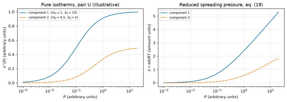
Results
6.1 The mixture equilibria (the construction of Figs. 3, 4 — illustrative)
The \((y{-}x)\) diagram and the total amount adsorbed for pair U, at three total pressures. These have the structure of the paper’s Figs. 3 and 4 — an azeotrope-free \(y{-}x\) curve bowed toward the strongly adsorbed component, \(n_t\) falling as the weakly adsorbed component takes over the gas — but they are computed from the illustrative parameters and reproduce nothing in the paper; the paper’s own curves would need the Szepesy & Illés isotherms this page does not have.
yfine = np.linspace(1e-3, 1-1e-3, 399)
fig, ax = plt.subplots(1, 2, figsize=(10.5, 3.9))
for Pt, ls in [(0.2, ":"), (1.0, "-"), (5.0, "--")]:
    s = iast(Pt, yfine, pU1, pU2)
    ax[0].plot(s["x1"], yfine, ls, color="C0", label=f"$P = {Pt:g}$")
    ax[1].plot(yfine, s["nt"], ls, color="C0", label=f"$P = {Pt:g}$")
ax[0].plot([0, 1], [0, 1], lw=0.8, color="0.5")
ax[0].set(xlabel="$x_1$ (adsorbed phase)", ylabel="$y_1$ (gas phase)",
          title="$y{-}x$ diagram, pair U (illustrative)")
ax[0].legend(fontsize=8)
ax[1].set(xlabel="$y_1$ (gas phase)", ylabel="$n_t$ (amount units)",
          title="Total amount adsorbed, eq. (26)")
ax[1].legend(fontsize=8)
fig.tight_layout(); plt.show()
S_RESULTS = {Pt: iast(Pt, yfine, pU1, pU2) for Pt in (0.2, 1.0, 5.0)}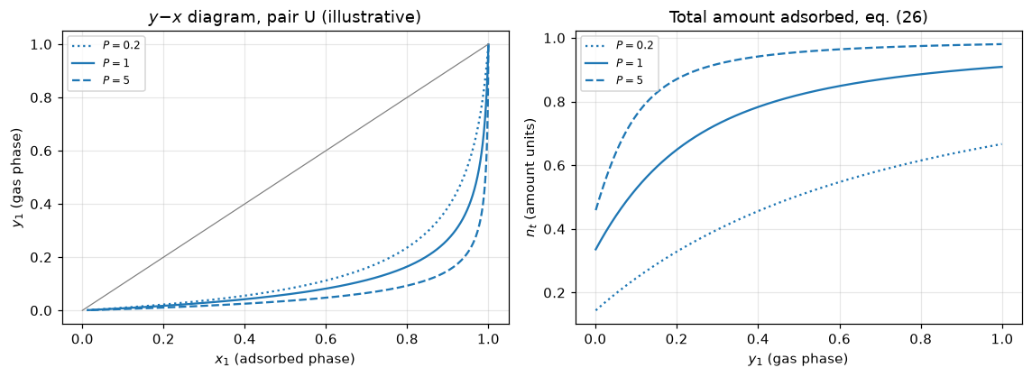
6.2 The paper’s graphical procedure, drawn and checked (Fig. 1’s construction)
The paper’s general algorithm is geometric: at a chosen spreading pressure the horizontal line \(ABC\) cuts the two pure \(z(P)\) curves at \(B = (P_1^{\circ}, z^{*})\) and \(C = (P_2^{\circ}, z^{*})\); a point \(D\) on \(BC\) picks the mixture pressure; the chords \(OB\), \(OC\) and the vertical through \(D\) give \(E\) and \(F\); and eqs. (45), (46) read the equilibrium off the ruler: \(y_1 = \mathrm{DE}/\mathrm{FE}\), \(x_1 = \mathrm{DC}/\mathrm{BC}\). §2.1 proved both symbolically; here the construction is drawn for pair U and the lever rules evaluated numerically — the same numbers the Newton solver returns, which is eq. (44) and the ruler agreeing about eq. (40).
ZSTAR, X1STAR = 1.2, 0.85
P1s, P2s = float(pU1["Pinv"](ZSTAR)), float(pU2["Pinv"](ZSTAR))
Pd = P1s*X1STAR + P2s*(1 - X1STAR)                    # eq. (29): D chosen via x1
Fh, Eh = ZSTAR*Pd/P1s, ZSTAR*Pd/P2s                   # chords OB, OC at abscissa Pd
y1_lever = (ZSTAR - Eh)/(Fh - Eh)                     # eq. (45)
x1_lever = (P2s - Pd)/(P2s - P1s)                     # eq. (46)
y1_direct = P1s*X1STAR/Pd                             # eq. (22)
LEVER_DEV = max(abs(y1_lever - y1_direct), abs(x1_lever - X1STAR))
# and the defect that shows the check has power: swap the chords
Fs, Es = ZSTAR*Pd/P2s, ZSTAR*Pd/P1s
LEVER_SWAPPED = abs((ZSTAR - Es)/(Fs - Es) - y1_direct)

Pc = np.geomspace(1e-3, P2s*1.08, 300)
fig, ax = plt.subplots(figsize=(7.6, 4.6))
ax.plot(Pc, pU1["z"](Pc), color="C0", label="pure component 1")
ax.plot(Pc, pU2["z"](Pc), color="C1", label="pure component 2")
ax.plot([0, P2s], [ZSTAR, ZSTAR], "k--", lw=0.8)
ax.plot([0, Pd], [0, Fh], "k:", lw=0.8)                 # chord OB extended to F
ax.plot([0, P2s], [0, ZSTAR], "k:", lw=0.8)             # chord OC
ax.plot([Pd, Pd], [0, Fh], "k--", lw=0.8)
for x_, z_, nm, off in [(0, ZSTAR, "A", (-11, 4)), (P1s, ZSTAR, "B", (-3, 6)),
                        (P2s, ZSTAR, "C", (4, 4)), (Pd, ZSTAR, "D", (4, 5)),
                        (Pd, Eh, "E", (5, -11)), (Pd, Fh, "F", (5, 1))]:
    ax.plot(x_, z_, "ko", ms=4)
    ax.annotate(nm, (x_, z_), textcoords="offset points", xytext=off, fontsize=10)
ax.set(xlabel="$P$ (arbitrary units)", ylabel="$z = \\pi A/RT$",
       title=f"Fig. 1's construction, computed: $y_1 = $ DE/FE $ = {y1_lever:.6f}$,"
             f"  $x_1 = $ DC/BC $ = {x1_lever:.6f}$",
       xlim=(0, P2s*1.08), ylim=(0, Fh*1.12))
ax.legend(fontsize=8, loc="center right")
fig.tight_layout(); plt.show()
print(f"lever rules vs eqs. (22)/(29) directly: max deviation {LEVER_DEV:.1e}")
print(f"with the chords deliberately swapped:   {LEVER_SWAPPED:.4f}  (the check can fail)")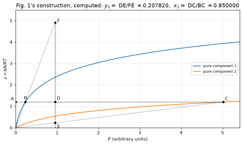
lever rules vs eqs. (22)/(29) directly: max deviation 1.1e-16
with the chords deliberately swapped:   0.5844  (the check can fail)
6.3 Selectivity: what varies, what cannot (the structure of Fig. 10’s claim)
The paper’s Fig. 10 discussion is the one place it exhibits IAST predicting a composition-dependent selectivity — “a small composition dependence” the data of Bering and Serpenskii could not resolve. For pair U the dependence is anything but small, and both infinite-dilution ends have closed forms (the dilute-1 limit is \(s \to P/P_1^{\circ}(z_2(P))\), the dilute-2 limit \(s \to P_2^{\circ}(z_1(P))/P\); at \(P = 1\) these evaluate to \(5(1+\sqrt3) = 13.660254\) and exactly \(60\)), so the page reports limits, not sampled extrema. For pair L the selectivity is \(b_1/b_2 = 10\) identically — under IAST, any two pure isotherms that are the same curve shifted in \(\log P\) give exactly constant selectivity (§7.8 proves and breaks this) — so composition dependence of \(s\) under IAST measures the two isotherms’ difference in shape, not in scale. The paper does not state this; its Henry-limit section (eqs. 30–35, constant \(s = K_1/K_2\)) is the linear special case of it.
# closed-form dilution limits at P = 1 (pair U)
P_ = 1.0
S_DIL1 = float(P_/pU1["Pinv"](pU2["z"](P_)))          # y1 -> 0
S_DIL2 = float(pU2["Pinv"](pU1["z"](P_))/P_)          # y1 -> 1
S_DIL_RATIO = S_DIL2/S_DIL1
fig, ax = plt.subplots(figsize=(7.2, 4.0))
for Pt, ls in [(0.2, ":"), (1.0, "-"), (5.0, "--")]:
    s = S_RESULTS[Pt]
    ax.plot(yfine, s["s12"], ls, color="C0", label=f"pair U, $P = {Pt:g}$")
ax.plot(1e-3, S_DIL1, "o", color="C3", ms=6, zorder=5)
ax.plot(1-1e-3, S_DIL2, "o", color="C3", ms=6, zorder=5,
        label="closed-form dilution limits, $P{=}1$")
sL = iast(1.0, yfine, pL1, pL2)
ax.plot(yfine, sL["s12"], "-", color="C2", lw=1.2,
        label="pair L (equal shape): $s \\equiv b_1/b_2 = 10$")
ax.set(xlabel="$y_1$ (gas phase)", ylabel="selectivity $s_{1,2}$, eq. (28)", yscale="log",
       title="Selectivity under IAST: shape difference, not scale, drives the variation")
ax.legend(fontsize=8)
fig.tight_layout(); plt.show()
print(f"pair U at P = 1: dilute-in-1 limit s = {S_DIL1:.6f} = 5(1+sqrt(3)) = {5*(1+np.sqrt(3)):.6f}")
print(f"                 dilute-in-2 limit s = {S_DIL2:.6f} (exactly 60: e^(2 ln 11) = 121, (121-1)/2)")
print(f"                 composition-dependence factor {S_DIL_RATIO:.6f}")
SEL_EQUAL_M_SPREAD = float(np.ptp(sL["s12"][np.isfinite(sL["s12"])])/np.nanmean(sL["s12"]))
print(f"pair L: relative spread of s over the whole composition range {SEL_EQUAL_M_SPREAD:.2e}")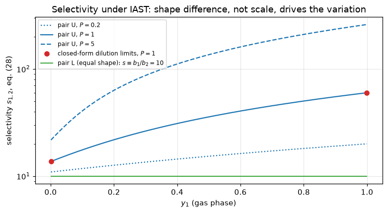
pair U at P = 1: dilute-in-1 limit s = 13.660254 = 5(1+sqrt(3)) = 13.660254
                 dilute-in-2 limit s = 60.000000 (exactly 60: e^(2 ln 11) = 121, (121-1)/2)
                 composition-dependence factor 4.392305
pair L: relative spread of s over the whole composition range 3.16e-12
# The page's computed reference table, written for reuse (see the data sidecar:
# COMPUTED output, not data from any paper). Deterministic across runs.
rows = []
for pair, (q1, q2) in [("L", (pL1, pL2)), ("U", (pU1, pU2))]:
for Pt in (0.2, 1.0, 5.0):
yv = np.round(np.arange(0.1, 0.91, 0.1), 10)
s = iast(Pt, yv, q1, q2)
for i, yy in enumerate(yv):
rows.append((pair, Pt, yy, s["z"][i], s["x1"][i], s["nt"][i],
s["n1"][i], s["n2"][i], s["s12"][i]))
ref = pd.DataFrame(rows, columns=["pair", "P", "y1", "z", "x1", "n_t", "n_1", "n_2", "s12"])
Path("data").mkdir(exist_ok=True)
hdr = ("# IAST reference solutions COMPUTED BY PAGE J1.4 on two illustrative Langmuir pairs.\n"
"# NOT experimental data and NOT from Myers & Prausnitz (1965); see the .meta.yaml sidecar.\n"
"# pair L: m=1, b1=10, b2=1. pair U: m1=1, b1=10, m2=0.5, b2=2. Arbitrary units.\n")
with open("data/iast-illustrative-reference.csv", "w", encoding="utf-8") as fh:
fh.write(hdr)
ref.to_csv(fh, index=False, float_format="%.12g")
print(f"wrote data/iast-illustrative-reference.csv ({len(ref)} rows)")
ref.head(6)wrote data/iast-illustrative-reference.csv (54 rows)| pair | P | y1 | z | x1 | n_t | n_1 | n_2 | s12 | |
|---|---|---|---|---|---|---|---|---|---|
| 0 | L | 0.2 | 0.1 | 0.322083 | 0.526316 | 0.275362 | 0.144928 | 0.130435 | 10.0 |
| 1 | L | 0.2 | 0.2 | 0.444686 | 0.714286 | 0.358974 | 0.256410 | 0.102564 | 10.0 |
| 2 | L | 0.2 | 0.3 | 0.553885 | 0.810811 | 0.425287 | 0.344828 | 0.080460 | 10.0 |
| 3 | L | 0.2 | 0.4 | 0.652325 | 0.869565 | 0.479167 | 0.416667 | 0.062500 | 10.0 |
| 4 | L | 0.2 | 0.5 | 0.741937 | 0.909091 | 0.523810 | 0.476190 | 0.047619 | 10.0 |
| 5 | L | 0.2 | 0.6 | 0.824175 | 0.937500 | 0.561404 | 0.526316 | 0.035088 | 10.0 |
Validation
Eight numerical sections. Every reported metric appears in §7.9’s defect-injection table with a row that moves it, or is explicitly labelled structural/below-floor there with an above-floor companion named. Since nothing here is experimental, every check below is a consistency test of the theory’s printed structure and of this page’s solver — none is evidence that IAST describes any real system.
7.1 The solver against a closed form it never touches (equal capacities)
§2.1 derived symbolically that for equal-capacity Langmuir pairs the IAST solution is the extended Langmuir rule. The Newton solver knows nothing of that closed form — it solves the spreading-pressure match by iteration — so agreement is a real test of the whole chain (matching, eq. (22), eq. (26)).
Pgrid, ygrid = np.meshgrid(np.geomspace(0.01, 10, 30), np.linspace(0.02, 0.98, 30))
GP, GY = Pgrid.ravel(), ygrid.ravel()

def eqm_dev(p1_, p2_, m1_, b1_, m2_, b2_, tol=1e-13):
    s = iast(GP, GY, p1_, p2_, tol=tol)
    n1e, n2e = ext_langmuir(GP, GY, m1_, b1_, m2_, b2_)
    return float(np.max(np.abs(np.array([s["n1"] - n1e, s["n2"] - n2e]))
                        / np.maximum(n1e + n2e, 1e-300)))

EQM_DEV = eqm_dev(pL1, pL2, mL, b1L, mL, b2L)
print(f"IAST solver vs extended-Langmuir closed form, pair L, 900 states: "
      f"max rel dev {EQM_DEV:.3e}")
print("(solver-tolerance level; below the CI floor of 1e-12 -- named as such in 7.9,")
print(" with the three break rows below as its above-floor companions)")

# break rows -- the same comparison must MOVE when the premise is broken
BRK_EQM_M2   = eqm_dev(pL1, langmuir_pure(0.6, b2L), mL, b1L, mL, b2L)   # unequal capacity
BRK_EQM_B1   = eqm_dev(langmuir_pure(mL, 1.01*b1L), pL2, mL, b1L, mL, b2L)  # 1 % wrong b1
BRK_EQM_TOL  = eqm_dev(pL1, pL2, mL, b1L, mL, b2L, tol=1e-3)             # loose Newton
print(f"\nbreaks:  m2 = 0.6            -> {BRK_EQM_M2:.3f}")
print(f"         b1 off by 1 %       -> {BRK_EQM_B1:.3e}")
print(f"         Newton tol 1e-3     -> {BRK_EQM_TOL:.3e}")
IAST solver vs extended-Langmuir closed form, pair L, 900 states: max rel dev 7.635e-16
(solver-tolerance level; below the CI floor of 1e-12 -- named as such in 7.9,
with the three break rows below as its above-floor companions)
breaks: m2 = 0.6 -> 0.424
b1 off by 1 % -> 9.081e-03
Newton tol 1e-3 -> 2.441e-107.2 Where extended Langmuir stops being an IAST (unequal capacities)
With \(m_1 \ne m_2\) the two models genuinely differ, and the size of the difference is this page’s first physical statement. Both extrema are computed honestly: the deviation grows monotonically with \(P\) across the window (asserted below), so its supremum sits on the window’s \(P = 10\) edge and is a window supremum by definition, not a sampled maximum; the interior maximum over \(y_1\) at that edge is root-found (a 30-point grid read would have been 0.7 % low — printed beside it); and the dilute-component deviation has a closed form at \(y_1 \to 0\), where both models are linear in \(y_1\) and the ratio of slopes is \(\bigl[m_1 b_1 P/(1{+}b_2 P)\bigr] \big/ \bigl[(P/P_1^{\circ}(z_2(P)))\,n_2^{\circ}(P)\bigr]\).
def nt_dev_U(y, Pt):
    s = iast(np.array([Pt]), np.array([y]), pU1, pU2)
    n1e, n2e = ext_langmuir(np.array([Pt]), np.array([y]), m1U, b1U, m2U, b2U)
    return float(abs((n1e + n2e) - s["nt"])[0]/s["nt"][0])

# monotone in P at the (P-wise) optimal y -- so the window sup is at P = 10
Pchecks = np.array([0.5, 1.0, 2.0, 5.0, 10.0])
maxdev_at_P = []
for Pt in Pchecks:
    r = minimize_scalar(lambda y: -nt_dev_U(y, Pt), bounds=(1e-3, 1-1e-3),
                        method="bounded", options=dict(xatol=1e-12))
    maxdev_at_P.append(-r.fun)
assert np.all(np.diff(maxdev_at_P) > 0), "monotone growth with P across the window"

r = minimize_scalar(lambda y: -nt_dev_U(y, 10.0), bounds=(1e-3, 1-1e-3),
                    method="bounded", options=dict(xatol=1e-13))
NT_DEV_SUP, NT_DEV_Y = -r.fun, float(r.x)
sU = iast(GP, GY, pU1, pU2)
n1e, n2e = ext_langmuir(GP, GY, m1U, b1U, m2U, b2U)
NT_DEV_GRID = float(np.max(np.abs((n1e + n2e) - sU["nt"])/sU["nt"]))

# dilute-component deviation, closed form at y1 -> 0, P = 10
Pt = 10.0
slope_EL   = m1U*b1U*Pt/(1.0 + b2U*Pt)
slope_IAST = (Pt/pU1["Pinv"](pU2["z"](Pt)))*pU2["n"](Pt)
N1_DILUTE_DEV = float(abs(slope_EL/slope_IAST - 1.0))

print(f"n_t deviation, window sup (P = 10 edge, y1 root-found): {NT_DEV_SUP:.6f} at y1* = {NT_DEV_Y:.6f}")
print(f"  the 30 x 30 grid read of the same quantity: {NT_DEV_GRID:.6f}  "
      f"({100*(1 - NT_DEV_GRID/NT_DEV_SUP):.2f} % low -- why extrema are root-found here)")
print(f"dilute-component-1 deviation at P = 10, closed form: {N1_DILUTE_DEV:.6f}")

# break: restore m2 = m1 and both must collapse
sB = iast(GP, GY, pU1, langmuir_pure(m1U, b2U))
n1b, n2b = ext_langmuir(GP, GY, m1U, b1U, m1U, b2U)
BRK_NT_EQUALM = float(np.max(np.abs((n1b + n2b) - sB["nt"])/sB["nt"]))
slope_IAST_eq = (Pt/pU1["Pinv"](langmuir_pure(m1U, b2U)["z"](Pt)))*langmuir_pure(m1U, b2U)["n"](Pt)
BRK_N1_EQUALM = float(abs(m1U*b1U*Pt/(1.0 + b2U*Pt)/slope_IAST_eq - 1.0))
print(f"\nbreak (m2 -> m1): window measure collapses to {BRK_NT_EQUALM:.2e}, "
      f"dilute closed form to {BRK_N1_EQUALM:.2e}")
n_t deviation, window sup (P = 10 edge, y1 root-found): 0.215079 at y1* = 0.099555
the 30 x 30 grid read of the same quantity: 0.213643 (0.67 % low -- why extrema are root-found here)
dilute-component-1 deviation at P = 10, closed form: 0.641742
break (m2 -> m1): window measure collapses to 6.52e-16, dilute closed form to 0.00e+007.3 The Henry-law limit — the one case the paper proves rigorous
Eqs. (30)–(35): at vanishing coverage IAST must reproduce \(n_i = K_i P y_i\) and the constant selectivity \(K_1/K_2\). Two tests. (a) On pure Henry isotherms the solver must be exact at any pressure — it is, to solver tolerance. (b) On pair U the selectivity must converge to \(K_1/K_2 = m_1 b_1 / m_2 b_2 = 10\) as \(P \to 0\), at first order in \(P\) (the leading correction to both isotherms is \(O(P)\)); the observed order over six decades is printed.
# (a) pure Henry isotherms: closed case of eqs. (30)-(35)
KH1, KH2 = 3.0, 0.7
yv = np.linspace(0.05, 0.95, 11)
sH = iast(0.37, yv, henry_pure(KH1), henry_pure(KH2))
HENRY_EXACT = float(np.max(np.abs(sH["n1"] - KH1*0.37*yv)/(KH1*0.37*yv)))
print(f"(a) solver on pure Henry isotherms vs n1 = K1 P y1 (eq. 31): max rel {HENRY_EXACT:.2e}")
print("    (below the CI floor; its above-floor companion is the no-matching break below)")
# break: skip the spreading-pressure matching entirely (x_i = y_i)
n1_nomatch = yv/(yv/(KH1*0.37) + (1 - yv)/(KH2*0.37))
BRK_HENRY_NOMATCH = float(np.max(np.abs(n1_nomatch - KH1*0.37*yv)/(KH1*0.37*yv)))
print(f"    break (matching skipped, x_i = y_i): {BRK_HENRY_NOMATCH:.3f}")

# (b) pair U selectivity -> K1/K2 at first order
S_INF = (m1U*b1U)/(m2U*b2U)
Psweep = 10.0**np.arange(-3, -9, -1)
hdev = np.array([abs(float(iast(p, np.array([0.5]), pU1, pU2)["s12"][0])/S_INF - 1.0)
                 for p in Psweep])
orders = np.log10(hdev[:-1]/hdev[1:])
HENRY_DEV = float(hdev[-1]); HENRY_ORDER = float(orders[-1])
print(f"\n(b) |s/ (K1/K2) - 1| at P = 1e-3 ... 1e-8: " +
      "  ".join(f"{d:.2e}" for d in hdev))
print(f"    observed order in P: {HENRY_ORDER:.4f}  (first order, as the O(P) isotherm "
      f"correction requires)")
# breaks
BRK_HENRY_P01 = abs(float(iast(0.1, np.array([0.5]), pU1, pU2)["s12"][0])/S_INF - 1.0)
BRK_HENRY_WRONGK = abs((b1U/b2U)/S_INF - 1.0)
hdev_wrong = np.abs(np.array([float(iast(p, np.array([0.5]), pU1, pU2)["s12"][0]) for p in Psweep])
                    /(b1U/b2U) - 1.0)
BRK_HENRY_ORDER = float(np.log10(hdev_wrong[-2]/hdev_wrong[-1]))
print(f"    breaks: read at P = 0.1 instead -> {BRK_HENRY_P01:.4f};  K = b (capacity "
      f"forgotten) -> {BRK_HENRY_WRONGK:.2f};")
print(f"            order against that wrong limit -> {BRK_HENRY_ORDER:.4f} (convergence gone)")
(a) solver on pure Henry isotherms vs n1 = K1 P y1 (eq. 31): max rel 2.17e-16
(below the CI floor; its above-floor companion is the no-matching break below)
break (matching skipped, x_i = y_i): 0.757
(b) |s/ (K1/K2) - 1| at P = 1e-3 ... 1e-8: 2.75e-03 2.75e-04 2.75e-05 2.75e-06 2.75e-07 2.75e-08
observed order in P: 1.0000 (first order, as the O(P) isotherm correction requires)
breaks: read at P = 0.1 instead -> 0.2697; K = b (capacity forgotten) -> 0.50;
order against that wrong limit -> 0.0000 (convergence gone)7.4 The general spreading-pressure quadrature, refined and broken
Eq. (19) for isotherms known only pointwise: log-grid trapezoid with the Henry segment \([0, t_0]\) added analytically as \(K t_0\) — the low-coverage care the paper’s conclusions single out. Tested against the analytic \(z = m\ln(1+bP)\) on pair U’s component 1; the error must fall at second order in the node count, and the two design choices (log grid, Henry anchor) each get a break row.
def z_quad(Pp, nfun, K_, n_nodes=257, t0_frac=1e-8):
    t0 = t0_frac*Pp
    tg = np.geomspace(t0, Pp, n_nodes)
    return K_*t0 + np.trapezoid(nfun(tg), np.log(tg))     # eq. (19): n d ln t

ZA = pU1["z"](1.0)
qerr = {nn: abs(z_quad(1.0, pU1["n"], pU1["K"], nn)/ZA - 1.0) for nn in (65, 129, 257, 513)}
QUAD_ERR = float(qerr[257])
QUAD_ORDER = float(np.log2(qerr[257]/qerr[513]))
print("nodes -> rel err: " + "   ".join(f"{k}: {v:.3e}" for k, v in qerr.items()))
print(f"reported: rel err at 257 nodes {QUAD_ERR:.3e}, observed order {QUAD_ORDER:.4f}")

# breaks
BRK_QUAD_LIN = abs(np.trapezoid(pU1["n"](np.linspace(1e-8, 1, 257))
                                / np.linspace(1e-8, 1, 257), np.linspace(1e-8, 1, 257))/ZA - 1.0)
def z_quad_noanchor(nn, t0_frac=1e-3):
    tg = np.geomspace(t0_frac, 1.0, nn)
    return np.trapezoid(pU1["n"](tg), np.log(tg))
BRK_QUAD_NOANCHOR = abs(z_quad_noanchor(257)/ZA - 1.0)
BRK_QUAD_NOANCHOR_ORDER = float(np.log2(abs(z_quad_noanchor(257)/ZA - 1.0)
                                        / abs(z_quad_noanchor(513)/ZA - 1.0)))
WITH_ANCHOR_SAME_T0 = abs((pU1["K"]*1e-3 + z_quad_noanchor(257))/ZA - 1.0)
print(f"breaks: linear grid, same 257 nodes      -> {BRK_QUAD_LIN:.3e}")
print(f"        Henry anchor dropped (t0 = 1e-3) -> {BRK_QUAD_NOANCHOR:.3e}, "
      f"observed order {BRK_QUAD_NOANCHOR_ORDER:.3f} (truncation-dominated, convergence gone;")
print(f"        restoring the anchor at the same t0 recovers {WITH_ANCHOR_SAME_T0:.3e})")
nodes -> rel err: 65: 2.378e-04 129: 5.947e-05 257: 1.487e-05 513: 3.718e-06
reported: rel err at 257 nodes 1.487e-05, observed order 2.0000
breaks: linear grid, same 257 nodes -> 5.254e-05
Henry anchor dropped (t0 = 1e-3) -> 4.148e-03, observed order -0.000 (truncation-dominated, convergence gone;
restoring the anchor at the same t0 recovers 2.256e-05)7.5 The Gibbs adsorption isotherm along a path — eq. (21) as a solver test
At constant \(T\) and \(P\), eq. (21) says \(\;(A/RT)\,d\pi = n_1\,d\ln y_1 + n_2\,d\ln y_2\). The left side comes from the solver’s \(z(y_1)\) — the pure-component route, eq. (19) at the matched \(P_i^{\circ}\) — while the right side integrates the mixture amounts along the composition path. The two routes share the solve but not the thermodynamics: if the solver returned self-consistent but wrong states (mismatched spreading pressures, or a wrong \(n_t\) rule), the identity fails, and the break rows show exactly that — the arithmetic-mean \(n_t\) (the plausible wrong reading of eq. (26)) misses by 1.5 %, and a 1 % mismatch between the two components’ spreading pressures by 0.16 %.
YA, YB = 0.05, 0.95
zA = float(iast(1.0, np.array([YA]), pU1, pU2)["z"][0])
zB = float(iast(1.0, np.array([YB]), pU1, pU2)["z"][0])
DZ = zB - zA

def path_rhs_gauss(ng):
    xg, wg = leggauss(ng)
    yv_ = 0.5*(YB - YA)*xg + 0.5*(YA + YB)
    s = iast(1.0, yv_, pU1, pU2)
    return 0.5*(YB - YA)*float(np.sum(wg*(s["n1"]/yv_ - s["n2"]/(1 - yv_))))

def iast_defect(Pt, y1v, zfac2=1.0, nt_mode="harmonic"):
    """The pair-U IAST solve with an injectable defect: the two components'
    spreading pressures mismatched by zfac2 (a broken eq. 40), and/or eq. (26)
    read as an ARITHMETIC mean (the plausible wrong reading)."""
    Pt = np.broadcast_to(np.asarray(Pt, float), np.shape(y1v)).ravel().copy()
    y1v = np.asarray(y1v, float).ravel()
    jacd = NumJac((y1v.size, 1))
    def res(wc):
        zz = np.exp(wc[:, 0])
        return (Pt*y1v/pU1["Pinv"](zz) + Pt*(1-y1v)/pU2["Pinv"](zfac2*zz) - 1.0)[:, None]
    z0 = np.maximum(pU1["z"](Pt), pU2["z"](Pt))
    so = newton(lambda wc: jacd(res, wc), np.log(z0).reshape(-1, 1), tol=1e-13, maxfev=200)
    assert so.success
    zz = np.exp(so.x[:, 0])
    P1v, P2v = pU1["Pinv"](zz), pU2["Pinv"](zfac2*zz)
    x1v = Pt*y1v/P1v
    n1o, n2o = pU1["n"](P1v), pU2["n"](P2v)
    ntv = (x1v*n1o + (1-x1v)*n2o) if nt_mode == "arith" else 1.0/(x1v/n1o + (1-x1v)/n2o)
    return dict(z=zz, x1=x1v, nt=ntv, n1=x1v*ntv, n2=(1-x1v)*ntv)

def path_rhs_trap(nn, nt_mode="harmonic", zfac2=1.0):
    yv_ = np.linspace(YA, YB, nn)
    s = (iast(1.0, yv_, pU1, pU2) if nt_mode == "harmonic" and zfac2 == 1.0
         else iast_defect(1.0, yv_, zfac2=zfac2, nt_mode=nt_mode))
    return float(np.trapezoid(s["n1"]/yv_ - s["n2"]/(1 - yv_), yv_))

PATH_GAUSS = abs(path_rhs_gauss(64) - DZ)/abs(DZ)
t65, t129 = abs(path_rhs_trap(65) - DZ)/abs(DZ), abs(path_rhs_trap(129) - DZ)/abs(DZ)
PATH_TRAP65, PATH_TRAP_ORDER = float(t65), float(np.log2(t65/t129))
print(f"pure-route Delta z = {DZ:.10f}   (P = 1, y1: {YA} -> {YB})")
print(f"mixture-route integral: Gauss-64 residual {PATH_GAUSS:.2e} (below CI floor -- named in 7.9;")
print(f"                        trapezoid-65 residual {PATH_TRAP65:.3e} is the CI-active metric,")
print(f"                        observed order {PATH_TRAP_ORDER:.4f})")

# breaks
DZ_MM = (float(iast_defect(1.0, np.array([YB]), zfac2=1.01)["z"][0])
         - float(iast_defect(1.0, np.array([YA]), zfac2=1.01)["z"][0]))
BRK_PATH_ARITH = abs(path_rhs_trap(4001, nt_mode="arith") - DZ)/abs(DZ)
BRK_PATH_MISMATCH = abs(path_rhs_trap(4001, zfac2=1.01) - DZ_MM)/abs(DZ_MM)
a65 = abs(path_rhs_trap(65, nt_mode="arith") - DZ)/abs(DZ)
a129 = abs(path_rhs_trap(129, nt_mode="arith") - DZ)/abs(DZ)
BRK_PATH_ARITH_ORDER = float(np.log2(a65/a129))
print(f"\nbreaks (both on 4001-node trapezoids, so quadrature error is negligible):")
print(f"  n_t read as the ARITHMETIC mean of eq. (26)     -> residual {BRK_PATH_ARITH:.3e}")
print(f"  spreading pressures mismatched by 1 % (eq. 40)  -> residual {BRK_PATH_MISMATCH:.3e}")
print(f"  and the order under the arithmetic defect: {BRK_PATH_ARITH_ORDER:.3f} "
      f"(saturates -- refinement cannot fix a wrong identity)")
pure-route Delta z = 1.6051451807 (P = 1, y1: 0.05 -> 0.95)
mixture-route integral: Gauss-64 residual 4.15e-16 (below CI floor -- named in 7.9;
trapezoid-65 residual 8.776e-05 is the CI-active metric,
observed order 1.9999)
breaks (both on 4001-node trapezoids, so quadrature error is negligible):
n_t read as the ARITHMETIC mean of eq. (26) -> residual 1.520e-02
spreading pressures mismatched by 1 % (eq. 40) -> residual 1.597e-03
and the order under the arithmetic defect: 0.006 (saturates -- refinement cannot fix a wrong identity)7.6 The closed loop: the paper’s consistency charge, quantified
The paper reports (p. 125) that Bering and Serpenskii “noted that the Langmuir equation for mixture adsorption was not thermodynamically consistent”. Here is that sentence as a number. If a mixture model \(n_i(P, y_1)\) respects the Gibbs adsorption isotherm, the one-form \(n_t\,d\ln P + (n_1/y_1 - n_2/y_2)\,dy_1\) is exact and its integral around any closed loop vanishes — \(\pi\) is a state function. Around the rectangle \(P \in [0.2, 1]\), \(y_1 \in [0.2, 0.8]\):
- IAST closes the loop to machine precision, as its construction from a single \(\pi\) guarantees in exact arithmetic — but not in code: the same loop with the two components’ spreading pressures mismatched by 1 % (a solver bug this test would catch) fails at \(2\times10^{-3}\).
- Extended Langmuir with unequal capacities does not close: the deficit is 12 % of the loop’s own spreading-pressure scale. Computed twice, by routes sharing no assembly — the boundary line integral of the model’s \(n_i\), and the area integral of the curl that §2.1 derived symbolically (\((m_2{-}m_1) b_1 b_2 P^2/D^2\)) — agreeing to 2.7e-15. The curl’s closed form makes the deficit exactly linear in \(m_2 - m_1\) (its denominator contains no \(m\)), and doubling \(m_1 - m_2\) doubles the measured loop deficit to machine precision, a third route to the same structure. At \(m_2 = m_1\) everything vanishes identically — the consistent case is exactly the case where extended Langmuir is an IAST (§2.1, §7.1).
LOOP = dict(Pa=0.2, Pb=1.0, ya=0.2, yb=0.8)

def circulation(model, ngauss=48, skip_edge4=False, **loop):
    Pa, Pb, ya, yb = loop.get("Pa", 0.2), loop.get("Pb", 1.0), loop.get("ya", 0.2), loop.get("yb", 0.8)
    xg, wg = leggauss(ngauss)
    lnv = 0.5*(np.log(Pb) - np.log(Pa))*xg + 0.5*(np.log(Pa) + np.log(Pb))
    yv_ = 0.5*(yb - ya)*xg + 0.5*(ya + yb)
    tot = 0.0
    n1_, n2_ = model(np.exp(lnv), np.full_like(lnv, ya))
    tot += 0.5*(np.log(Pb) - np.log(Pa))*np.sum(wg*(n1_ + n2_))          # bottom, ->
    n1_, n2_ = model(np.full_like(yv_, Pb), yv_)
    tot += 0.5*(yb - ya)*np.sum(wg*(n1_/yv_ - n2_/(1 - yv_)))            # right, ^
    n1_, n2_ = model(np.exp(lnv), np.full_like(lnv, yb))
    tot -= 0.5*(np.log(Pb) - np.log(Pa))*np.sum(wg*(n1_ + n2_))          # top, <-
    if not skip_edge4:
        n1_, n2_ = model(np.full_like(yv_, Pa), yv_)
        tot -= 0.5*(yb - ya)*np.sum(wg*(n1_/yv_ - n2_/(1 - yv_)))        # left, v
    return float(tot)

model_iast_U = lambda Pt, yv_: (lambda s: (s["n1"], s["n2"]))(iast(Pt, yv_, pU1, pU2))
model_extL_U = lambda Pt, yv_: ext_langmuir(Pt, yv_, m1U, b1U, m2U, b2U)

CIRC_IAST = circulation(model_iast_U)
CIRC_EXTL = circulation(model_extL_U)
Z_SCALE = float(pU1["z"](LOOP["Pb"]) - pU1["z"](LOOP["Pa"]))    # the loop's own z scale
CIRC_REL = CIRC_EXTL/Z_SCALE

# route 2: Green's theorem with the symbolically derived curl
xg, wg = leggauss(48)
lnv = 0.5*(np.log(1.0) - np.log(0.2))*xg + 0.5*(np.log(0.2) + np.log(1.0))
yv_ = 0.5*(0.8 - 0.2)*xg + 0.5*(0.2 + 0.8)
LN, YV = np.meshgrid(lnv, yv_)
W2 = np.outer(wg, wg)*0.25*(np.log(1.0) - np.log(0.2))*(0.8 - 0.2)
CIRC_GREEN = float(np.sum(W2*curl_fn(LN, YV, m1U, b1U, m2U, b2U)))
ROUTE_AGREE = abs(CIRC_EXTL/CIRC_GREEN - 1.0)

# route 3: exact linearity in (m2 - m1)
CIRC_DOUBLE = circulation(lambda Pt, yv2: ext_langmuir(Pt, yv2, m1U, b1U, 0.0, b2U))
LINEARITY = CIRC_DOUBLE/CIRC_EXTL          # (0 - 1)/(0.5 - 1) = 2 exactly
LINEARITY_DEV = abs(LINEARITY - 2.0)

print(f"loop deficit, IAST:               {abs(CIRC_IAST):.2e}   (closes; below CI floor, named in 7.9)")
print(f"loop deficit, extended Langmuir:  {CIRC_EXTL:.6f}  =  {100*CIRC_REL:.2f} % of the "
      f"loop's z-scale {Z_SCALE:.6f}")
print(f"same deficit via the symbolic curl (Green route): {CIRC_GREEN:.6f}   "
      f"routes agree to {ROUTE_AGREE:.2e}")
print(f"doubling m1 - m2 multiplies the deficit by {LINEARITY:.15f}  (exactly 2 in exact arithmetic)")

# breaks
model_mismatch = lambda Pt, yv2: (lambda s: (s["n1"], s["n2"]))(iast_defect(Pt, yv2, zfac2=1.01))
BRK_CIRC_MISMATCH = abs(circulation(model_mismatch))
BRK_CIRC_EQUALM = abs(circulation(lambda Pt, yv2: ext_langmuir(Pt, yv2, m1U, b1U, m1U, b2U)))
BRK_ROUTE_G2 = abs(circulation(model_extL_U, ngauss=2)/CIRC_GREEN - 1.0)
BRK_LIN_EDGE4 = abs(circulation(lambda Pt, yv2: ext_langmuir(Pt, yv2, m1U, b1U, 0.0, b2U),
                                skip_edge4=True)
                    / circulation(model_extL_U, skip_edge4=True) - 2.0)
print(f"\nbreaks: 1 % spreading-pressure mismatch injected into IAST -> loop deficit "
      f"{BRK_CIRC_MISMATCH:.2e}")
print(f"        m2 -> m1 in extended Langmuir -> deficit {BRK_CIRC_EQUALM:.2e} (collapses)")
print(f"        line-integral route on 2-point Gauss -> route agreement degrades to {BRK_ROUTE_G2:.2e}")
print(f"        edge 4 of the loop dropped -> linearity factor off by {BRK_LIN_EDGE4:.3f}")
loop deficit, IAST: 7.77e-16 (closes; below CI floor, named in 7.9)
loop deficit, extended Langmuir: -0.154834 = -11.92 % of the loop's z-scale 1.299283
same deficit via the symbolic curl (Green route): -0.154834 routes agree to 2.66e-15
doubling m1 - m2 multiplies the deficit by 2.000000000000002 (exactly 2 in exact arithmetic)
breaks: 1 % spreading-pressure mismatch injected into IAST -> loop deficit 1.97e-03
m2 -> m1 in extended Langmuir -> deficit 5.00e-16 (collapses)
line-integral route on 2-point Gauss -> route agreement degrades to 6.10e-03
edge 4 of the loop dropped -> linearity factor off by 1.2897.7 The lever rules, numerically (their symbolic proof is §2.1)
An identity in exact arithmetic — the numeric check is kept because it is what §6.2’s drawing rests on, and because its break (chords swapped, the plausible mis-drawing of Fig. 1) moves the answer by order one.
print(f"lever rules vs eqs. (22)/(29): max deviation {LEVER_DEV:.2e} "
      f"(identically zero here; below CI floor, named in 7.9)")
print(f"break -- chords OB and OC swapped: {LEVER_SWAPPED:.4f}")
lever rules vs eqs. (22)/(29): max deviation 1.11e-16 (identically zero here; below CI floor, named in 7.9)
break -- chords OB and OC swapped: 0.58447.8 The shape-translation result: when IAST selectivity cannot vary
Claim (this page’s, not the paper’s): if the two pure isotherms are the same curve shifted in \(\log P\) — \(n_2^{\circ}(P) = n_1^{\circ}(\kappa P)\) — then eq. (19) gives \(\pi_2(P^{\circ}) = \pi_1(\kappa P^{\circ})\), the match (40) forces \(P_1^{\circ} = \kappa P_2^{\circ}\), and the selectivity (28) is exactly \(1/\kappa\), independent of \(P\) and composition. The Henry-limit constancy of eqs. (30)–(35) is the linear special case (any two lines are shape-identical, \(\kappa = K_2/K_1\)); §6.3’s pair L is the equal-capacity Langmuir case (\(\kappa = b_2/b_1\)). Searched for in the paper and not found there: the Fig. 10 discussion (pp. 125–126) treats the composition dependence as a prediction to compare with data, and the conclusions do not connect selectivity constancy to isotherm shape; the closest printed statement is the Henry-limit special case itself. Verified here on pair S — dual-site isotherms the closed forms of §7.1 never see, inverted numerically — and broken by perturbing one site’s affinity so the shapes genuinely differ.
Pg2, yg2 = np.meshgrid(np.geomspace(0.05, 5, 12), np.linspace(0.1, 0.9, 12))
sS = iast(Pg2.ravel(), yg2.ravel(), pS1, pS2)
selS = sS["s12"]
SHAPE_SPREAD = float(np.ptp(selS)/np.mean(selS))
print(f"pair S (same shape, kappa = {KAPPA}): selectivity mean {np.mean(selS):.12f} "
      f"vs 1/kappa = {1/KAPPA}")
print(f"  relative spread over 144 states spanning 100x in P: {SHAPE_SPREAD:.2e} "
      f"(below CI floor, named in 7.9)")

# break: perturb ONE site of component 2 by 5 % -- shapes now differ
pS2_pert = dualsite_pure(0.7, 20.0, 0.3, 0.5*1.05, KAPPA)
sSp = iast(Pg2.ravel(), yg2.ravel(), pS1, pS2_pert)
SHAPE_PERT_SPREAD = float(np.ptp(sSp["s12"])/np.mean(sSp["s12"]))
print(f"break -- one site's b perturbed 5 %: spread {SHAPE_PERT_SPREAD:.3e} "
      f"(the constancy is the shape identity, not the solver)")

# dilution-limit second route for 6.3's closed forms: solver at y1 = 1e-8
S_DIL1_SOLVER = float(iast(1.0, np.array([1e-8]), pU1, pU2)["s12"][0])
DIL1_ROUTE_DEV = abs(S_DIL1_SOLVER/S_DIL1 - 1.0)
BRK_DIL1_Y01 = abs(float(iast(1.0, np.array([0.1]), pU1, pU2)["s12"][0])/S_DIL1 - 1.0)
print(f"\n6.3's dilute-in-1 closed form checked by the solver at y1 = 1e-8: "
      f"rel dev {DIL1_ROUTE_DEV:.2e}")
print(f"break -- read at y1 = 0.1 instead of the limit: {BRK_DIL1_Y01:.3f}")
# and the ratio's break: equal-shape pair has ratio exactly 1
S_DIL_RATIO_L = float((pL2["Pinv"](pL1["z"](1.0))/1.0) / (1.0/pL1["Pinv"](pL2["z"](1.0))))
print(f"composition-dependence factor, pair U: {S_DIL_RATIO:.6f};  pair L (equal shape): "
      f"{S_DIL_RATIO_L:.6f} (collapses to 1)")
pair S (same shape, kappa = 0.25): selectivity mean 4.000000000000 vs 1/kappa = 4.0
relative spread over 144 states spanning 100x in P: 4.65e-14 (below CI floor, named in 7.9)
break -- one site's b perturbed 5 %: spread 1.067e-02 (the constancy is the shape identity, not the solver)
6.3's dilute-in-1 closed form checked by the solver at y1 = 1e-8: rel dev 2.68e-08
break -- read at y1 = 0.1 instead of the limit: 0.286
composition-dependence factor, pair U: 4.392305; pair L (equal shape): 1.000000 (collapses to 1)7.9 The defect-injection table, and the coverage map that builds itself
Every metric reported to agreement.json must have a row here that moves it, or be named below with its reason and an above-floor companion. The coverage map is assembled from the table itself (a metric cannot claim a row that is not in the table), and the assert fails the notebook on any mismatch in either direction.
BREAKS = [
    # metric, defect injected, baseline, broken value
    ("equal_m_closed_form_max_rel", "m2 = 0.6 (capacities made unequal)", EQM_DEV, BRK_EQM_M2),
    ("equal_m_closed_form_max_rel", "b1 wrong by 1 %", EQM_DEV, BRK_EQM_B1),
    ("equal_m_closed_form_max_rel", "Newton tol loosened to 1e-3", EQM_DEV, BRK_EQM_TOL),
    ("unequal_m_nt_dev_windowsup", "m2 -> m1 (models coincide again)", NT_DEV_SUP, BRK_NT_EQUALM),
    ("unequal_m_n1_dilute_limit_dev", "m2 -> m1, closed form", N1_DILUTE_DEV, BRK_N1_EQUALM),
    ("henry_model_solver_max_rel", "spreading-pressure matching skipped (x_i = y_i)",
     HENRY_EXACT, BRK_HENRY_NOMATCH),
    ("henry_selectivity_dev_P1em8", "read at P = 0.1 instead of the limit", HENRY_DEV, BRK_HENRY_P01),
    ("henry_selectivity_dev_P1em8", "Henry constant taken as b (capacity forgotten)",
     HENRY_DEV, BRK_HENRY_WRONGK),
    ("henry_convergence_order", "order measured against that wrong limit", HENRY_ORDER, BRK_HENRY_ORDER),
    ("pi_quadrature_rel_err_257", "linear grid instead of logarithmic", QUAD_ERR, BRK_QUAD_LIN),
    ("pi_quadrature_rel_err_257", "Henry anchor dropped (t0 = 1e-3)", QUAD_ERR, BRK_QUAD_NOANCHOR),
    ("pi_quadrature_observed_order", "Henry anchor dropped: order collapses",
     QUAD_ORDER, BRK_QUAD_NOANCHOR_ORDER),
    ("gibbs_path_trap65_rel", "n_t read as the arithmetic mean of eq. (26)",
     PATH_TRAP65, BRK_PATH_ARITH),
    ("gibbs_path_trap65_rel", "spreading pressures mismatched by 1 % (eq. 40)",
     PATH_TRAP65, BRK_PATH_MISMATCH),
    ("gibbs_path_trap_order", "arithmetic-mean defect: order saturates",
     PATH_TRAP_ORDER, BRK_PATH_ARITH_ORDER),
    ("gibbs_path_gauss64_rel", "arithmetic-mean defect (same rows as trap-65)",
     PATH_GAUSS, BRK_PATH_ARITH),
    ("loop_circulation_iast_abs", "1 % spreading-pressure mismatch injected",
     abs(CIRC_IAST), BRK_CIRC_MISMATCH),
    ("loop_circulation_ext_langmuir", "m2 -> m1: deficit collapses", CIRC_EXTL, BRK_CIRC_EQUALM),
    ("loop_circulation_ext_langmuir", "m2 -> 0: deficit exactly doubles", CIRC_EXTL, CIRC_DOUBLE),
    ("loop_circulation_over_scale", "same two rows (derived metric: deficit / z-scale)",
     CIRC_REL, BRK_CIRC_EQUALM/Z_SCALE),
    ("circulation_route_rel_agreement", "line-integral route degraded to 2-point Gauss",
     ROUTE_AGREE, BRK_ROUTE_G2),
    ("circulation_linearity_dev", "edge 4 of the loop dropped", LINEARITY_DEV, BRK_LIN_EDGE4),
    ("lever_rule_max_dev", "chords OB and OC swapped", LEVER_DEV, LEVER_SWAPPED),
    ("shape_translation_selectivity_rel_spread", "one site's affinity perturbed 5 %",
     SHAPE_SPREAD, SHAPE_PERT_SPREAD),
    ("shape_perturbed_selectivity_rel_spread", "perturbation removed (collapses back)",
     SHAPE_PERT_SPREAD, SHAPE_SPREAD),
    ("selectivity_dilute_ratio_P1", "equal-shape pair: factor collapses to 1",
     S_DIL_RATIO, S_DIL_RATIO_L),
    ("selectivity_dilute1_solver_vs_closed_rel", "read at y1 = 0.1 instead of the limit",
     DIL1_ROUTE_DEV, BRK_DIL1_Y01),
]
bt = pd.DataFrame(BREAKS, columns=["metric", "defect injected", "baseline", "broken"])
with pd.option_context("display.float_format", lambda v: f"{v:.3e}"):
    display(bt)

# --- structural / below-floor declarations, each with its companion --------
STRUCTURAL = {
    "sym_zero_identity_count": "a count of sympy identities; it verifies algebra, not numerics, "
        "and no runtime defect can move it -- cited as evidence for nothing numerical",
}
BELOW_FLOOR = {   # metric -> its above-floor companion (all companions are CI-active or in BREAKS)
    "equal_m_closed_form_max_rel":
        f"its three break rows ({BRK_EQM_M2:.2f}, {BRK_EQM_B1:.1e}, {BRK_EQM_TOL:.1e})",
    "henry_model_solver_max_rel": f"the no-matching break ({BRK_HENRY_NOMATCH:.2f})",
    "gibbs_path_gauss64_rel": "gibbs_path_trap65_rel (CI-active) and the arithmetic-mean break",
    "loop_circulation_iast_abs": "loop_circulation_ext_langmuir (CI-active) and the mismatch break",
    "circulation_route_rel_agreement": f"the 2-point-Gauss break ({BRK_ROUTE_G2:.1e})",
    "circulation_linearity_dev": f"the dropped-edge break ({BRK_LIN_EDGE4:.2f})",
    "lever_rule_max_dev": f"the swapped-chords break ({LEVER_SWAPPED:.2f}) and the symbolic proof in 2.1",
    "shape_translation_selectivity_rel_spread": "shape_perturbed_selectivity_rel_spread (CI-active)",
}
print("Below the CI comparison floor (1e-12) while healthy -- protected by their companions, "
      "not by CI:")
for k, v in BELOW_FLOOR.items():
    print(f"  {k}: companion = {v}")
print("Structural (no break row can exist):")
for k, v in STRUCTURAL.items():
print(f" {k}: {v}")| metric | defect injected | baseline | broken | |
|---|---|---|---|---|
| 0 | equal_m_closed_form_max_rel | m2 = 0.6 (capacities made unequal) | 7.635e-16 | 4.240e-01 |
| 1 | equal_m_closed_form_max_rel | b1 wrong by 1 % | 7.635e-16 | 9.081e-03 |
| 2 | equal_m_closed_form_max_rel | Newton tol loosened to 1e-3 | 7.635e-16 | 2.441e-10 |
| 3 | unequal_m_nt_dev_windowsup | m2 -> m1 (models coincide again) | 2.151e-01 | 6.517e-16 |
| 4 | unequal_m_n1_dilute_limit_dev | m2 -> m1, closed form | 6.417e-01 | 0.000e+00 |
| 5 | henry_model_solver_max_rel | spreading-pressure matching skipped (x_i = y_i) | 2.174e-16 | 7.574e-01 |
| 6 | henry_selectivity_dev_P1em8 | read at P = 0.1 instead of the limit | 2.750e-08 | 2.697e-01 |
| 7 | henry_selectivity_dev_P1em8 | Henry constant taken as b (capacity forgotten) | 2.750e-08 | 5.000e-01 |
| 8 | henry_convergence_order | order measured against that wrong limit | 1.000e+00 | 2.150e-07 |
| 9 | pi_quadrature_rel_err_257 | linear grid instead of logarithmic | 1.487e-05 | 5.254e-05 |
| 10 | pi_quadrature_rel_err_257 | Henry anchor dropped (t0 = 1e-3) | 1.487e-05 | 4.148e-03 |
| 11 | pi_quadrature_observed_order | Henry anchor dropped: order collapses | 2.000e+00 | -4.807e-04 |
| 12 | gibbs_path_trap65_rel | n_t read as the arithmetic mean of eq. (26) | 8.776e-05 | 1.520e-02 |
| 13 | gibbs_path_trap65_rel | spreading pressures mismatched by 1 % (eq. 40) | 8.776e-05 | 1.597e-03 |
| 14 | gibbs_path_trap_order | arithmetic-mean defect: order saturates | 2.000e+00 | 5.743e-03 |
| 15 | gibbs_path_gauss64_rel | arithmetic-mean defect (same rows as trap-65) | 4.150e-16 | 1.520e-02 |
| 16 | loop_circulation_iast_abs | 1 % spreading-pressure mismatch injected | 7.772e-16 | 1.969e-03 |
| 17 | loop_circulation_ext_langmuir | m2 -> m1: deficit collapses | -1.548e-01 | 4.996e-16 |
| 18 | loop_circulation_ext_langmuir | m2 -> 0: deficit exactly doubles | -1.548e-01 | -3.097e-01 |
| 19 | loop_circulation_over_scale | same two rows (derived metric: deficit / z-scale) | -1.192e-01 | 3.845e-16 |
| 20 | circulation_route_rel_agreement | line-integral route degraded to 2-point Gauss | 2.665e-15 | 6.097e-03 |
| 21 | circulation_linearity_dev | edge 4 of the loop dropped | 2.220e-15 | 1.289e+00 |
| 22 | lever_rule_max_dev | chords OB and OC swapped | 1.110e-16 | 5.844e-01 |
| 23 | shape_translation_selectivity_rel_spread | one site's affinity perturbed 5 % | 4.652e-14 | 1.067e-02 |
| 24 | shape_perturbed_selectivity_rel_spread | perturbation removed (collapses back) | 1.067e-02 | 4.652e-14 |
| 25 | selectivity_dilute_ratio_P1 | equal-shape pair: factor collapses to 1 | 4.392e+00 | 1.000e+00 |
| 26 | selectivity_dilute1_solver_vs_closed_rel | read at y1 = 0.1 instead of the limit | 2.675e-08 | 2.857e-01 |
Below the CI comparison floor (1e-12) while healthy -- protected by their companions, not by CI:
  equal_m_closed_form_max_rel: companion = its three break rows (0.42, 9.1e-03, 2.4e-10)
  henry_model_solver_max_rel: companion = the no-matching break (0.76)
  gibbs_path_gauss64_rel: companion = gibbs_path_trap65_rel (CI-active) and the arithmetic-mean break
  loop_circulation_iast_abs: companion = loop_circulation_ext_langmuir (CI-active) and the mismatch break
  circulation_route_rel_agreement: companion = the 2-point-Gauss break (6.1e-03)
  circulation_linearity_dev: companion = the dropped-edge break (1.29)
  lever_rule_max_dev: companion = the swapped-chords break (0.58) and the symbolic proof in 2.1
  shape_translation_selectivity_rel_spread: companion = shape_perturbed_selectivity_rel_spread (CI-active)
Structural (no break row can exist):
  sym_zero_identity_count: a count of sympy identities; it verifies algebra, not numerics, and no runtime defect can move it -- cited as evidence for nothing numerical
What pymrm adds
Nothing to the theory, and the page says so plainly: IAST is algebra plus one scalar root-find per state, and most of this notebook would run with pymrm uninstalled — exactly as on J1.1, J1.3 and A1.6. What newton and NumJac do here is narrow and real:
- The whole \((P, y_1)\) grid as one Newton problem. The spreading-pressure match is solved for hundreds of states simultaneously with
NumJac((K, 1))— independent scalars, a diagonal Jacobian by construction. The shape is(K, 1)and never(K,): the bare 1-D shape would couple every state to every other and build a dense \(K \times K\) Jacobian for no change in the answer (the house rule, measured onB1.1). The iteration runs in \(\ln z\), which is what keeps Newton on the feasible side of \(P^{\circ}(0) = 0\). - The general-isotherm inverse. For pair S the pure isotherms have no analytic inverse; \(P^{\circ}(z)\) is itself a vectorised
newtonsolve nested inside the IAST solve. That is the machinery a user with tabulated isotherms (eq. 43) actually needs. - Root-finds and closed forms where a sweep would have been wrong. The §7.2 supremum is root-found (the grid read is 0.7 % low — printed), the dilution limits are closed forms rather than end-of-grid reads, and the quadrature and path integrals carry observed orders, not single numbers.
The one thing on this page that is genuinely useful beyond reproduction is not pymrm at all: the closed-loop consistency test of §7.6 (with its symbolically derived curl) as a portable diagnostic. It applies to any proposed mixture-adsorption model \(n_i(P, y)\), needs no IAST solve, and returns a single number that is zero iff the model carries a consistent spreading pressure. The extended-Langmuir deficit — 12 % of scale on an ordinary parameter set — is what it reports on the most widely used shortcut model in the field, and the \(m_2 = m_1\) collapse identifies why the shortcut is safe exactly when capacities match.
Reuse
Use this page for a working, tested IAST solver (iast + langmuir_pure/dualsite_pure/henry_pure), the consistency-loop diagnostic (circulation), and the reference solutions in data/iast-illustrative-reference.csv for regression-testing your own implementation (parameters in the file header; equal-capacity pair L also has the closed form to check against).
Four things to carry away:
- Extended Langmuir is safe exactly when capacities match. Then it is the ideal adsorbed solution (§2.1, symbolically). With unequal capacities it is thermodynamically inconsistent — a 12 %-of-scale loop deficit on an unremarkable parameter set (§7.6) and a 21.5 % total-amount error against IAST at the illustrative window’s edge (§7.2) — and the dilute component is where it is worst (64 % there). If you must use it, check the capacity ratio first.
- Eq. (26) is a harmonic mix. The arithmetic reading is the natural slip and it fails the Gibbs isotherm by 1.5 % on this page’s mild example (§7.5) — a thermodynamic error, not a numerical one, so no grid refinement will ever surface it (§7.5’s order break shows the residual saturating).
- The low-pressure tail of the pure isotherms is load-bearing. The paper’s own conclusions say so; §7.4 quantifies it — dropping the Henry anchor at \(t_0 = 10^{-3}\) costs 4e-3 in \(z\) and kills the convergence order, so refinement looks converged while being wrong. Measure the Henry constant, or extrapolate to it explicitly, before integrating eq. (19).
- Composition-dependent selectivity is a shape signal. Under IAST, isotherms differing only by a \(\log P\) shift give exactly constant \(s_{1,2}\) (§7.8). If your IAST calculation shows strong composition dependence, your two pure isotherms differ in shape — and if your data show it where the fitted pure isotherms do not, IAST with those fits cannot represent the system, whatever the parameters.
Do not use this page as evidence that IAST works. It contains no experimental comparison — the paper’s four validation systems are figures of external data, out of scope here — and every agreement on it is structural. The empirical literature on IAST is enormous; this page is about what the 1965 paper actually established on its own printed content. Do not use it for dynamics — breakthrough is J1.5, and this page’s iast can serve as that page’s mixture-equilibrium closure. Do not read pairs L, U, S as any physical system; they are illustrative parameter sets and nothing more.
metrics = {
    "sym_zero_identity_count": SYM_ZERO_COUNT,
    "equal_m_closed_form_max_rel": EQM_DEV,
    "unequal_m_nt_dev_windowsup": NT_DEV_SUP,
    "unequal_m_n1_dilute_limit_dev": N1_DILUTE_DEV,
    "henry_model_solver_max_rel": HENRY_EXACT,
    "henry_selectivity_dev_P1em8": HENRY_DEV,
    "henry_convergence_order": HENRY_ORDER,
    "pi_quadrature_rel_err_257": QUAD_ERR,
    "pi_quadrature_observed_order": QUAD_ORDER,
    "gibbs_path_trap65_rel": PATH_TRAP65,
    "gibbs_path_trap_order": PATH_TRAP_ORDER,
    "gibbs_path_gauss64_rel": PATH_GAUSS,
    "loop_circulation_iast_abs": abs(CIRC_IAST),
    "loop_circulation_ext_langmuir": CIRC_EXTL,
    "loop_circulation_over_scale": CIRC_REL,
    "circulation_route_rel_agreement": ROUTE_AGREE,
    "circulation_linearity_dev": LINEARITY_DEV,
    "lever_rule_max_dev": LEVER_DEV,
    "shape_translation_selectivity_rel_spread": SHAPE_SPREAD,
    "shape_perturbed_selectivity_rel_spread": SHAPE_PERT_SPREAD,
    "selectivity_dilute_ratio_P1": S_DIL_RATIO,
    "selectivity_dilute1_solver_vs_closed_rel": DIL1_ROUTE_DEV,
}

# --- the coverage map builds itself from the break table -------------------
covered = set(bt["metric"])
declared = covered | set(STRUCTURAL)
assert set(metrics) == declared, (
    f"coverage mismatch: unclaimed={set(metrics)-declared}, phantom={declared-set(metrics)}")
moved = bt[abs(bt.broken - bt.baseline) > 0]
assert set(moved["metric"]) == covered, "a break row failed to move its metric"
print(f"coverage: {len(metrics)} metrics = {len(covered)} with moving break rows "
      f"+ {len(STRUCTURAL)} structural.  Assert passed in both directions.\n")

report_agreement("J1.4", metrics)
coverage: 22 metrics = 21 with moving break rows + 1 structural. Assert passed in both directions.
Agreement metrics for J1.4:
sym_zero_identity_count = 11
equal_m_closed_form_max_rel = 7.6355e-16
unequal_m_nt_dev_windowsup = 0.21508
unequal_m_n1_dilute_limit_dev = 0.64174
henry_model_solver_max_rel = 2.1743e-16
henry_selectivity_dev_P1em8 = 2.75e-08
henry_convergence_order = 1
pi_quadrature_rel_err_257 = 1.487e-05
pi_quadrature_observed_order = 2
gibbs_path_trap65_rel = 8.776e-05
gibbs_path_trap_order = 1.9999
gibbs_path_gauss64_rel = 4.15e-16
loop_circulation_iast_abs = 7.7716e-16
loop_circulation_ext_langmuir = -0.15483
loop_circulation_over_scale = -0.11917
circulation_route_rel_agreement = 2.6645e-15
circulation_linearity_dev = 2.2204e-15
lever_rule_max_dev = 1.1102e-16
shape_translation_selectivity_rel_spread = 4.6518e-14
shape_perturbed_selectivity_rel_spread = 0.010665
selectivity_dilute_ratio_P1 = 4.3923
selectivity_dilute1_solver_vs_closed_rel = 2.6754e-08{'page': 'J1.4',
'metrics': {'sym_zero_identity_count': 11.0,
'equal_m_closed_form_max_rel': 7.635453975501703e-16,
'unequal_m_nt_dev_windowsup': 0.21507876398405296,
'unequal_m_n1_dilute_limit_dev': 0.6417424305044159,
'henry_model_solver_max_rel': 2.174349832795058e-16,
'henry_selectivity_dev_P1em8': 2.7500014487813473e-08,
'henry_convergence_order': 0.9999997499762475,
'pi_quadrature_rel_err_257': 1.4870143879130993e-05,
'pi_quadrature_observed_order': 1.9999529168647325,
'gibbs_path_trap65_rel': 8.775985910945557e-05,
'gibbs_path_trap_order': 1.9999495810931398,
'gibbs_path_gauss64_rel': 4.1499910585415586e-16,
'loop_circulation_iast_abs': 7.771561172376096e-16,
'loop_circulation_ext_langmuir': -0.15483360141013042,
'loop_circulation_over_scale': -0.11916849778016288,
'circulation_route_rel_agreement': 2.6645352591003757e-15,
'circulation_linearity_dev': 2.220446049250313e-15,
'lever_rule_max_dev': 1.1102230246251565e-16,
'shape_translation_selectivity_rel_spread': 4.651834473179406e-14,
'shape_perturbed_selectivity_rel_spread': 0.010665083545773094,
'selectivity_dilute_ratio_P1': 4.392304845413265,
'selectivity_dilute1_solver_vs_closed_rel': 2.675426480358567e-08}}# Every number quoted in this page's MARKDOWN is re-derived here and compared
# against the live computation; any mismatch raises and fails the notebook.
def close(a, b, rtol=5e-3, atol=1e-15):
ok = abs(a - b) <= atol + rtol*abs(b)
if not ok:
raise AssertionError(f"prose drift: typed {a!r} vs computed {b!r}")
return True
AUDIT = [
# (typed in prose, computed live, rtol; rtol 0 means exact)
("7.6e-16 solver vs closed form (title, 7.1)", 7.6e-16, EQM_DEV, 5e-2),
("2.7e-15 two routes (title, 7.6)", 2.7e-15, ROUTE_AGREE, 8e-2),
("7.8e-16 IAST closes the loop (title, 7.6)", 7.8e-16, abs(CIRC_IAST), 3e-1),
("12 % of scale (title, 7.6, Reuse)", 0.12, abs(CIRC_REL), 2e-2),
("4.7e-14 shape spread (title, 7.8)", 4.7e-14, SHAPE_SPREAD, 3e-1),
("eleven identities (title, 2.1)", 11, SYM_ZERO_COUNT, 0),
("3 DOF, eq. (18) (model, data)", 3, 2 - 2 + 3, 0),
("4.6 volumes/year, ref. 5 (data)", 4.6, REF5_VOL_RATE, 1e-9),
("13.660254 dilute-1 limit (6.3)", 13.660254, S_DIL1, 1e-6),
("... equals 5(1+sqrt(3))", 13.660254, 5*(1 + np.sqrt(3)), 1e-6),
("60 dilute-2 limit (6.3)", 60.0, S_DIL2, 1e-9),
("pair L selectivity = 10 (6.3)", 10.0,
float(np.nanmean(iast(1.0, yfine, pL1, pL2)["s12"])), 1e-9),
("21.5 % window sup (7.2, Reuse)", 0.215079, NT_DEV_SUP, 1e-4),
("y1* of the sup (7.2 print)", 0.099555, NT_DEV_Y, 1e-3),
("0.7 % low grid read (7.2, 8)", 0.007, 1 - NT_DEV_GRID/NT_DEV_SUP, 5e-2),
("64 % dilute closed form (7.2, Reuse)", 0.641742, N1_DILUTE_DEV, 1e-4),
("2.75e-8 Henry deviation (7.3)", 2.75e-8, HENRY_DEV, 1e-2),
("first order in P (7.3)", 1.0, HENRY_ORDER, 2e-3),
("1.49e-5 quadrature error (7.4)", 1.49e-5, QUAD_ERR, 5e-3),
("second order (7.4)", 2.0, QUAD_ORDER, 3e-2),
("4e-3 anchor dropped (7.4, Reuse)", 4e-3, BRK_QUAD_NOANCHOR, 5e-2),
("8.78e-5 path residual (7.5)", 8.78e-5, PATH_TRAP65, 5e-3),
("second order (7.5)", 2.0, PATH_TRAP_ORDER, 3e-2),
("1.5 % arithmetic mean (7.5, Reuse)", 0.015, BRK_PATH_ARITH, 5e-2),
("0.16 % from 1 % mismatch (7.5)", 1.6e-3, BRK_PATH_MISMATCH, 5e-2),
("2e-3-level loop failure (7.6)", 2e-3, BRK_CIRC_MISMATCH, 5e-2),
("exact doubling (7.6)", 2.0, LINEARITY, 1e-9),
("1.1e-2 perturbed-shape spread (7.8)", 0.0107, SHAPE_PERT_SPREAD, 2e-2),
("4.392305 composition factor (6.3)", 4.392305, S_DIL_RATIO, 1e-5),
("collapses to 1 (7.8)", 1.0, S_DIL_RATIO_L, 1e-9),
("34 scalars transcribed (data)", 34, len(claims), 0),
]
for label, typed, computed, rt in AUDIT:
if rt == 0:
assert typed == computed, f"prose drift [{label}]: {typed} != {computed}"
else:
try:
close(typed, computed, rtol=rt)
except AssertionError as e:
raise AssertionError(f"[{label}] {e}") from None
print(f"prose audit: {len(AUDIT)} numbers re-derived and matched. "
"Any drift raises and fails the notebook.")prose audit: 31 numbers re-derived and matched. Any drift raises and fails the notebook.References
Myers, A. L. and Prausnitz, J. M. (1965). Thermodynamics of mixed-gas adsorption. AIChE Journal 11(1), 121–127. doi:10.1002/aic.690110125 — the paper, and the only document read for content. Identity confirmed from its own first page on a native-resolution render: the title, the by-line “A. L. MYERS and J. M. PRAUSNITZ / University of California, Berkeley, California”, the footnote “A. L. Myers is at the University of Pennsylvania, Philadelphia, Pennsylvania”, the running feet “Vol. 11, No. 1 / A.I.Ch.E. Journal / Page 121”, and the Wiley PDF margin naming the same DOI; the Wiley Subject metadata independently gives “AIChE Journal 1965.11:121-127”. Manuscript received April 24, 1964; revision received August 14, 1964; accepted August 19, 1964. pdfimages -list reports all seven pages as CCITT-G4 bilevel at 300 ppi native, so every numeric was read from a crop of a 300 ppi render at digit scale; the text layer was used only as a search index. (The seventh PDF page carries the start of the next article — Gabor, “Lateral Transport in a Fluidized-Packed Bed” — below Myers & Prausnitz’s reference list; nothing was read from it.)
Cited by the paper, not consulted, and no number here derives from them — these four are the sources of every experimental point in Figs. 3–10, which is exactly why the experimental case is out of this page’s scope:
Szepesy, L. and Illés, V. (1963). Acta Chim. Hung. 35, 37; ibid. p. 53; ibid. p. 245 (refs. 9–11) — the methane, ethane and mixture isotherms behind Figs. 2–4. Markham, E. C. and Benton, A. F. (1931). J. Am. Chem. Soc. 53, 497 (ref. 8) — the CO–O₂/silica data of Figs. 5–6 (the Fig. 6 legend’s “(1950)” contradicts this, the paper’s only Markham & Benton reference; see §4). Lewis, W. K., Gilliland, E. R., Chertow, B. and Hoffman, W. H. (1950). J. Am. Chem. Soc. 72, 1153 (ref. 7) — the propane–propylene/silica-gel data of Fig. 7. Bering, B. P. and Serpenskii, V. V. (1952). Zhur. Fiz. Khim. 26, 253 (ref. 2) — the ethylene–CO₂ equilibrium surface behind Figs. 8–10 (the reference and text spell “Serpenskii”; the three figure legends spell “SERPINSKII” — one surname, two transliterations, reported as an observation).
Also cited, not consulted: Arnold (1949), J. Am. Chem. Soc. 71, 104 — the liquid entropy model the paper supersedes; de Boer (1953); Hill (1949), J. Chem. Phys. 17, 520, and Hill (1960), Introduction to Statistical Mechanics — the adsorption thermodynamics and the low-coverage statistical mechanics behind eqs. (4), (30), (31); Young & Crowell (1962) — the mixed-gas-adsorption review. Ref. 5 (“Ibid, 63, 456 (1959)”) is cited nowhere in the paper’s running text and its “Ibid.” (= J. Chem. Phys.) cannot carry volume 63 in 1959 (ref. 4’s own pair puts that journal at vol. 17 in 1949, and it was at vol. 37 in 1962); J. Phys. Chem. 63 (1959) exists and carries Hill’s adsorption-definitions paper at p. 456 — that ref. 5 intends it is an inference, stated as one.
J1.1 (Langmuir 1918) and J1.3 (BET 1938) are the pure-isotherm siblings; both were read for this page and neither is loaded — no dataset of either page is used and no number of theirs is retyped here.