Langmuir 1918: the isotherm that could not have proved its own conclusion

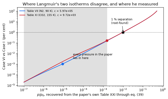
Langmuir’s isotherm is fitted to his own data by a hand-drawn straight line, so the agreement in Tables II-XVII is a goodness of fit and this page labels it as one everywhere. What can be tested is elsewhere, and there are two of them. Langmuir’s own contest against Freundlich is a fair one - two parameters each, the same eleven points - and Freundlich loses by a factor 3.82 in RMS on Table VII and on 13 of the 14 tables that can host the comparison, the single exception being the table Langmuir himself excludes. And the monomolecular conclusion does not rest on the isotherm at all: it rests on beta, the saturation amount against a monolayer count computed from the liquid density, whose worst row leaves only 17 % of headroom. The page’s own result is why that had to be so. Langmuir’s Case VI, eqs. (29) and (30) of the same paper, is shown by symbolic algebra to be EXACTLY the BET isotherm twenty years early; and every pressure he reached lies below p/p0 = 1.6e-3, where his monolayer and multilayer equations differ by at most 0.16 %, against observational scatter 12 to 1100 times larger. Four printed defects are reported and none repaired, including eq. (15)’s logarithm, which contradicts eq. (16) two lines below it; a fifth pattern, the sigma column running low, is reported separately because it is a truncation convention and not an error.

Langmuir 1918: the isotherm that could not have proved its own conclusion

Catalog ID: J1.1 · Structures: S1 (pointwise algebra) · Tier: T0

Everybody meets this paper as one equation,

\[\theta_1 \;=\; \frac{\sigma_1\mu}{1+\sigma_1\mu}, \qquad\text{equivalently}\qquad q \;=\; \frac{ab\,p}{1+ap}, \tag{9, 31}\]

and as the linear plot that fits it,

\[\frac{p}{q} \;=\; \frac{1}{ab} \;+\; \frac{p}{b}. \tag{32}\]

Langmuir obtained \(a\) and \(b\) by drawing a straight line as nearly as possible through the points of that plot. So the \(q_\mathrm{cal}\) columns of Tables II to XVII are a two-parameter fit compared against the two-parameter fit’s own training data. That is a goodness of fit. It is labelled one in every section of this page, it is never reported as an agreement metric, and a null baseline is printed beside it every time.

The paper’s real evidence is somewhere else, and this page is organised around finding it.

1. Langmuir stages a fair contest and wins it. Table VII carries two extra columns: Freundlich’s \(q_F = 8.4\,p^{0.417}\), fitted to the same eleven points with the same number of parameters. That is a discrimination, not a fit, because it can fail. Refitting both forms optimally — Langmuir’s drawn line is not the least-squares optimum, and neither is his Freundlich — the best two-parameter Freundlich is 3.82 times worse in RMS than the best two-parameter Langmuir on Table VII, and worse on 13 of the 14 tables with enough points to host the comparison. The one exception is Table XIII, which is the table Langmuir himself says does not satisfy eq. (31).
2. The monomolecular conclusion never rested on the isotherm. It rests on \(\beta\): the fitted saturation amount \(b\) converted to molecules per square centimetre through eq. (37), divided by the number in a close-packed layer computed from the liquid density — a conversion with no adsorption in it and nothing adjusted to make it come out below one. It comes out below one on all twenty entries, and the page reports the honest margin: the tightest row leaves 17 % of headroom.
3. And it could not have rested on the isotherm. This is the page’s own result and it is not in the paper. Langmuir’s Case VI — his multilayer theory, eqs. (26), (29) and (30), printed in the same paper — is shown here by symbolic algebra to be, with his own stated assumption \(\sigma_3=\sigma_4= \dots=\sigma_2\), exactly the BET isotherm, twenty years before Brunauer, Emmett and Teller wrote it down. Inverting the paper’s own Table XXI through eq. (3) recovers the saturation pressures Langmuir never prints, and every pressure in the entire paper lies below \(p/p_0 = 1.5\times10^{-3}\) — §6.9 computes that over every printed pressure, both bulbs and both isotherm forms, not only over the entries that can host a fit — where his monolayer and multilayer equations differ by at most 0.16 % — against observational scatter 12 to 1100 times larger. The isotherm shape was blind to the question the paper is about.

Four printed defects are reported and none repaired. The sharpest is eq. (15), whose logarithm contradicts eq. (16) two lines below it. A fifth pattern — the \(\sigma\) column running systematically low — is reported separately, because §6.3 identifies it as a truncation convention rather than an error.

Source. Langmuir, I. (1918). The Adsorption of Gases on Plane Surfaces of Glass, Mica and Platinum. J. Am. Chem. Soc. 40(9), 1361–1403, doi:10.1021/ja02242a004. Received June 25, 1918. Identity confirmed from its own title page on a native-resolution render — the contribution line “[Contribution from the Research Laboratory of the General Electric Co.]”, the title, the by-line “By Irving Langmuir”, “Received June 25, 1918”, and the ACS download stamp jacsat/article-pdf/40/9/1361/ printed down the margin of every page. PDF page 1 opens with the numbered summary of the preceding article (absorption spectra of metals in liquid ammonia); Langmuir’s title sits below it on the same page, and that is what was read.

pdfimages -list reports every page as CCITT-G4 bilevel at 300 ppi native, so pages were rendered at 300 ppi and every numeric cropped and re-read at digit scale. The text layer was not used for any digit, and that discipline was load-bearing here: the text layer renders eq. (37)’s coefficient as \(25.2\times10^{16}\) where the page prints \(25.2\times10^{\mathbf{15}}\) — a factor ten in every surface coverage on the page — and it mangled half the \(b\) column of Table X.

1. Background

What the paper is, and what this page takes from it

Forty-three journal pages, twenty-five tables. Most of it is an experimental campaign: outgassing bulbs, thermal-effusion corrections, and — from journal page 1393 on — irreversible chemisorption on platinum, which has no isotherm in it at all. The isotherm is a small part.

Scope decision, taken before transcription. This page is about the isotherm and the constants derived from it: the theory of journal pages 1368–1376 (Cases I–VI, eqs. 1–33) and Tables II–XI, XIII–XXII, which are the mica and glass isotherms and everything Langmuir computes from them. Table XXV is carried for one reason only — it exercises eq. (37) on a third adsorbent — and Tables I, XII, XXIII and XXIV (outgassing inventories and the platinum oxygen/carbon monoxide bookkeeping) are scoped out and not transcribed. They are excellent self-checking tables, but they are about the apparatus and about chemisorption, not about the isotherm.

That decision was taken the way the brief asks: prefer whatever lets you test rather than restate. Restating \(q_\mathrm{cal}\) would be restating a fit. The testable content is the discrimination against Freundlich, the \(\beta\) bound, and the internal identity web that ties \(a\) and \(b\) to \(\sigma\), \(N_0\) and \(\beta\) through five printed equations.

The theory, in the order Langmuir builds it

The kinetic picture is one sentence long: molecules striking a bare surface condense, molecules on the surface evaporate, and equilibrium is the balance. Eq. (1)/(2) give the impingement rate, eq. (4) is the balance, eq. (5) is the site inventory, and eqs. (6)–(9) are the isotherm. Then he generalises in five directions, each of which he calls a Case:

Case	assumption	result
I	one kind of site, one molecule per site	eq. (9), the Langmuir isotherm
II	several kinds of site, fractions \(\beta_1,\beta_2,\dots\)	eq. (19), a sum of Langmuir terms
III	a continuum of site types (amorphous solid)	eq. (21), an integral
IV	\(n\) molecules per site	eq. (26), a ratio of two polynomials
V	dissociative adsorption, two sites per molecule	eq. (28), \(\eta \propto \sqrt{p}\)
VI	films more than one molecule thick	eqs. (26), (29), (30)

Case VI is the one this page is going to press on. Langmuir writes: “The problem is then identical with that considered under Case IV. Equations 22, 23 and 24 are applicable without alteration and the solution of the problem is thus given by Equation 26.” — and then, because both series become infinite, he transforms eq. (26) into eq. (29), whose coefficients are eq. (30).

He also derives a rate: eq. (14) is the ODE for the approach to equilibrium, eq. (15) its integral, and eq. (16) the half-period. The paper never measures a rate, so this is theory only — but it is checkable against itself, and it does not survive the check.

The other thing in the paper: what Langmuir is arguing against

Journal page 1375 states the rival explicitly. Freundlich’s \(q = a p^{1/n}\) “agrees very poorly with experiment when the range of pressures is large”, and Langmuir explains why on his own theory: at low pressure eq. (9) is linear (\(1/n \to 1\)), at high pressure it saturates (\(1/n \to 0\)), so a single power law must fail at one end or the other. Then, in Table VII, he fits Freundlich to his own data and prints the residuals beside his own. That contest is reproduced here — with both forms refitted optimally, because neither of his fits is the least-squares optimum and a rival should be beaten at its best.

2. The published model

All equation numbers are Langmuir’s. Every one below was read off a 300 ppi crop.

Impingement. With \(p\) in bars (dynes per sq. cm.), \(R = 83.2\times10^6\) erg per degree,

\[\mu \;=\; \frac{p}{\sqrt{2\pi MRT}} \;=\; 43.75\times10^{-6}\,\frac{p}{\sqrt{MT}}. \tag{2, 3}\]

Case I. With \(\alpha\) the condensation coefficient, \(\nu_1\) the evaporation rate from a full surface, \(\theta\) bare and \(\theta_1\) covered,

\[\alpha\theta\mu = \nu_1\theta_1, \qquad \theta+\theta_1 = 1, \qquad \sigma_1 \equiv \frac{\alpha}{\nu_1}, \tag{4, 5, 7}\]

\[\frac{N}{N_0}\,\eta \;=\; \theta_1 \;=\; \frac{\sigma_1\mu}{1+\sigma_1\mu}, \qquad N = 6.06\times10^{23}. \tag{9}\]

Lives, and the approach to equilibrium.

\[\tau \;=\; \frac{N_0\alpha}{N\nu_1} \;=\; \frac{N_0\sigma_1}{N}, \qquad \eta \;=\; \frac{\tau\mu}{1+\sigma_1\mu}, \qquad \eta_\infty = \frac{\tau}{\sigma_1} = \frac{N_0}{N}; \tag{10, 11, 13}\]

\[\frac{N_0}{N}\frac{d\theta'}{dt} \;=\; \alpha\mu - (\nu_1+\alpha\mu)\theta', \tag{14}\]

\[t \;=\; \frac{N_0}{N\nu_1(1+\sigma_1\mu)}\,\ln\frac{\theta'}{\theta_1-\theta'}, \qquad t_{1/2} \;=\; \frac{\tau\ln 2}{\alpha(1+\sigma_1\mu)}. \tag{15, 16}\]

Eq. (15) is quoted exactly as printed. §6.7 shows it cannot be right and that eq. (16) — which Langmuir obtains from it — is.

Case II (several kinds of site) and the two-stage special case:

\[\frac{N\eta}{N_0} = \frac{\beta_1\sigma_1\mu}{1+\sigma_1\mu} + \frac{\beta_2\sigma_2\mu}{1+\sigma_2\mu} + \dots, \qquad q = b_1 + \frac{a_2b_2\,p}{1+a_2p}. \tag{19, 33}\]

Cases IV and VI (the multilayer ladder). With \(\sigma_n = \alpha_n/\nu_n\),

\[\frac{N\eta}{N_0} = \frac{\sigma_1\mu + 2\sigma_1\sigma_2\mu^2 + 3\sigma_1\sigma_2\sigma_3\mu^3 + \dots} {1 + \sigma_1\mu + \sigma_1\sigma_2\mu^2 + \sigma_1\sigma_2\sigma_3\mu^3 + \dots} \;=\; \frac{\sigma_1}{1/\mu + a + b\mu + c\mu^2 + \dots}, \tag{26, 29}\]

\[a = \sigma_1 - 2\sigma_2,\quad b = \sigma_2(4\sigma_2 - 3\sigma_3 - \sigma_1),\quad c = 2\sigma_2(6\sigma_2\sigma_3 - 2\sigma_3\sigma_4 + \sigma_1\sigma_2 - \sigma_1\sigma_3 - 4\sigma_2^2). \tag{30}\]

The fitted form and its linearisation.

\[q = \frac{ab\,p}{1+ap}, \qquad \frac{p}{q} = \frac{1}{ab} + \frac{p}{b}. \tag{31, 32}\]

What \(a\) and \(b\) mean. Dividing (31) by \(b\) and comparing with (9), and using \(1\ \text{cu. mm.} = 4.16\times10^{-8}\) gram molecules at 20 °C and 760 mm,

\[\sigma\mu = ap,\qquad N_0q = bN\eta,\qquad \eta = 4.16\times10^{-8}\,q/s, \tag{34, 35, 36}\]

\[\boxed{\;N_0 = 25.2\times10^{15}\,b/s\;} \qquad\text{and}\qquad \boxed{\;\sigma = 22860\,a\sqrt{MT}\;} \tag{37, 38}\]

with \(s\) the adsorbent area in sq. cm. Eq. (37) reads \(10^{15}\) on the page and \(10^{16}\) in the PDF’s text layer. Everything downstream — \(N_0\), \(\beta\), the monomolecular conclusion — is a factor ten different between the two.

Saturation. For a liquid in equilibrium with its own vapour, eq. (4) becomes \(\alpha\mu = \nu\), i.e.

\[\sigma\mu \;=\; 1 \quad\text{at saturation}. \tag{39}\]

Eq. (39) is what makes Table XXI invertible, and it is the paper’s own statement of the relation this page uses to recover \(p_0\).

# Colab environment cell
try:
    import pymrm  # noqa: F401
except ImportError:
    %pip install -q pymrm
try:
    import gallery_utils  # noqa: F401
except ImportError:
    %pip install -q "pymrm-gallery-utils @ git+https://github.com/computational-chemical-engineering/pymrm-gallery.git#subdirectory=shared" || None
    import sys, pathlib
    for _p in (pathlib.Path.cwd(), *pathlib.Path.cwd().parents):
        if (_p / "shared" / "gallery_utils.py").is_file():
            sys.path.insert(0, str(_p / "shared")); break
    import gallery_utils  # noqa: F401

ERROR: pymrm-gallery-utils @ git+https://github.com/computational-chemical-engineering/pymrm-gallery.git#subdirectory=shared from git+https://github.com/computational-chemical-engineering/pymrm-gallery.git#subdirectory=shared does not appear to be a Python project: neither 'setup.py' nor 'pyproject.toml' found.


/bin/bash: line 1: None: command not found

Note: you may need to restart the kernel to use updated packages.

import warnings

import numpy as np
import pandas as pd
import sympy as sp
import matplotlib.pyplot as plt
from decimal import Decimal
from scipy.optimize import brentq, minimize_scalar

from pymrm import newton, NumJac
from gallery_utils import Claims, load_data, load_meta

warnings.filterwarnings("ignore")
np.random.seed(0)          # nothing here is stochastic; seeded so two runs are identical
PAGE = "J1.1-langmuir-isotherm"
pd.set_option("display.width", 200)

RES = {}                   # every number quoted in prose lands here and is audited in cell 22
def keep(k, v):
    RES[k] = float(v)
    return v

print("pymrm", __import__("pymrm").__version__)

pymrm 3.2.0

3. Parameters and assumptions

Units, and the one that trips people. Langmuir’s bar is a dyne per square centimetre, not the modern \(10^5\) Pa. His summary says the work used “pressures of 100 bars (approximately 0.1 mm of mercury) or less”; the cell below checks that against the definition of a millimetre of mercury and reports the result. Amounts \(q\) are cubic millimetres of gas at 20 °C and 760 mm.

Constants used. Only Langmuir’s own, and each is verified against the definition it came from rather than assumed:

symbol	printed	where
\(R\)	\(83.2\times10^6\) erg deg\(^{-1}\)	journal p. 1368
coefficient of eq. (3)	\(43.75\times10^{-6}\)	eq. (3)
\(N\)	\(6.06\times10^{23}\)	eq. (9)
1 cu. mm. at 20 °C, 760 mm	\(4.16\times10^{-8}\) gram mol	journal p. 1389
coefficient of eq. (37)	\(25.2\times10^{15}\)	eq. (37)
coefficient of eq. (38)	\(22860\)	eq. (38)
mica surface \(s\)	5750 sq. cm.	journal p. 1376
glass surface \(s\)	1966 sq. cm.	journal p. 1386
platinum surface \(s\)	312 sq. cm.	journal p. 1393

Those seven numeric constants are not independent: \(43.75\times10^{-6}\) must be \(1/\sqrt{2\pi R}\), \(22860\) must be its reciprocal, \(4.16\times10^{-8}\) must be \(p_0V/RT\) at 20 °C and 760 mm, and \(25.2\times10^{15}\) must be \(N\) times that. None of the four is free, and checking them is the cheapest possible test that the transcription is right and that eq. (37) really carries \(10^{15}\).

Molecular weights are taken as Langmuir’s contemporaries would have: N₂ 28, CH₄ 16, CO 28, Ar 39.9, O₂ 32, CO₂ 44. The one that matters is argon — 39.9, not the modern 39.95 — and the difference moves \(\sigma\) by 0.06 %, far inside the rounding of the printed \(\sigma\) column.

Assumptions this page makes and the paper does not state.

• Table XXII’s combining rule. Where a gas has two or three adsorbed \(\sigma\) at one condition, the paper does not say how they were combined into one ratio. §6.4 measures which mean reproduces the printed cells rather than assuming one.
• The mica area applies to every mica table. Verified rather than assumed: §6.3 recovers \(s\) independently from each row.

What is external. Exactly one thing: the monolayer counts of journal page 1391 (\(0.66,\,0.63,\,0.66,\,0.77,\,0.77,\,0.61 \times 10^{15}\) per sq. cm.) come from the liquid densities, and only nitrogen’s molecular volume (35.5 cu. cm.) is printed. The other four are recovered in §6.5 by inverting the printed counts, and are labelled recoveries wherever they appear. That external input is precisely what makes \(\beta\) a test and not a fit.

# --- the constant chain: none of these four numbers is free ---------------
R = 83.2e6                     # erg per degree, journal p. 1368
NAV = 6.06e23                  # eq. (9)
K3 = 43.75e-6                  # eq. (3)
K37 = 25.2e15                  # eq. (37)   <-- 10^15 on the page, 10^16 in the text layer
K38 = 22860.0                  # eq. (38)
CUMM = 4.16e-8                 # gram molecules per cu. mm. at 20 C and 760 mm, p. 1389
S_CM2 = {"mica": 5750.0, "glass": 1966.0, "platinum": 312.0}
MW = {"N2": 28.0, "CH4": 16.0, "CO": 28.0, "Ar": 39.9, "O2": 32.0, "CO2": 44.0}
MMHG = 13.5951 * 980.665 * 0.1  # dyn/cm2 per MILLIMETRE of Hg (rho g h, h = 0.1 cm)
ATM = 760.0 * MMHG

chain = []
chain.append(("eq. (3) coefficient = 1/sqrt(2 pi R)", 1 / np.sqrt(2 * np.pi * R), K3))
chain.append(("eq. (38) coefficient = 1/(eq. 3 coefficient)", 1 / K3, K38))
chain.append(("1 cu.mm at 20 C, 760 mm = pV/RT", ATM * 1e-3 / (R * 293.15), CUMM))
chain.append(("eq. (37) coefficient = N x 4.16e-8", NAV * CUMM, K37))
ch = pd.DataFrame(chain, columns=["identity", "derived", "printed"])
ch["rel_pct"] = (ch.printed / ch.derived - 1) * 100
print(ch.to_string(index=False, float_format=lambda v: f"{v:.6g}"))
keep("chain_max_rel_pct", ch.rel_pct.abs().max())

# eq. (37) with the TEXT LAYER's exponent instead of the page's
keep("eq37_textlayer_factor", 25.2e16 / K37)
print(f"\nworst residual in the constant chain: {RES['chain_max_rel_pct']:.4f} %")
print(f"the text layer's 25.2e16 would multiply every N0 and beta on this page by "
      f"{RES['eq37_textlayer_factor']:.0f} and push most of them above the monolayer bound; "
      f"HOW MANY is not typed here, it is COUNTED in section 6.5 from the data")

# the bar unit, from Langmuir's own parenthesis
keep("hundred_bars_in_mmHg", 100 / MMHG)
print(f"\n100 bars = {RES['hundred_bars_in_mmHg']:.4f} mm Hg, printed as "
      f'"approximately 0.1 mm of mercury" (journal p. 1402)')

                                    identity     derived   printed    rel_pct
        eq. (3) coefficient = 1/sqrt(2 pi R) 4.37369e-05 4.375e-05  0.0298586
eq. (38) coefficient = 1/(eq. 3 coefficient)     22857.1     22860     0.0125
             1 cu.mm at 20 C, 760 mm = pV/RT 4.15435e-08  4.16e-08   0.135917
          eq. (37) coefficient = N x 4.16e-8 2.52096e+16  2.52e+16 -0.0380807

worst residual in the constant chain: 0.1359 %
the text layer's 25.2e16 would multiply every N0 and beta on this page by 10 and push most of them above the monolayer bound; HOW MANY is not typed here, it is COUNTED in section 6.5 from the data

100 bars = 0.0750 mm Hg, printed as "approximately 0.1 mm of mercury" (journal p. 1402)

4. The data

Five CSVs, all transcribed from this paper alone. No other page’s dataset is loaded, so none of the cross-page reconciliation obligations apply. No curve is digitised and no figure is used for anything — the paper’s only figure with content is Fig. 1, a schematic checkerboard of surface atoms with no numbers on it. No page image is committed anywhere.

file	contents
langmuir-1918-isotherms.csv	every \((p, q_\mathrm{obs}, q_\mathrm{cal})\) of Tables II–XI and XIII–XVII, both bulbs
langmuir-1918-constants.csv	the fitted \(a\), \(b\) per table joined to the derived columns of Tables XVIII–XX
langmuir-1918-lives.csv	Table XXI (liquefied-gas lives) and Table XXII (the ratios)
langmuir-1918-platinum-N0.csv	Table XXV, carried only to exercise eq. (37) on a third adsorbent
langmuir-1918-printed-claims.csv	the 36 scalars that live in prose, equations or table headers

Tier 5, not 6, and the distinction matters here. The \(q_\mathrm{obs}\) column is a measurement — pressures read on a McLeod gauge and gas volumes obtained by difference. Everything else in the paper (\(a\), \(b\), \(b'\), \(\sigma\), \(N_0\), \(\beta\), Tables XXI, XXII, XXV) is a constant Langmuir derived from those measurements, so reproducing one of those is reproduction, never validation, and the page says so at every such comparison.

Three things the source page says about its own rows, all of which affect us.

1. The mica results are uncorrected. Journal page 1385: “The results therefore obtained from bulb A are to be considered as being 10 to 30 % too high”, because the blank bulb A′ adsorbed measurably and no subtraction was made. Every mica \(\beta\) below is therefore an over-estimate, which is the direction that helps Langmuir’s conclusion — noted at §6.5.
2. One point is disowned. Journal page 1384: the \(q\) at \(p = 12.8\) in Table IX “is undoubtedly in error, as it cannot be made to fit into a smooth curve”. It is kept in the CSV, flagged here, and §6.6 reports the discrimination with and without it.
3. The blank bulb went negative. The largest negative “adsorption” recorded is \(-0.7\) cu. mm. (Table XVII), which is the paper’s own scale for its measurement error and is used as such below.

A completeness check before anything else. Tables XVIII–XX carry a “Number of obs.” column. It must equal the number of Bulb A rows this page transcribed for that table. Twenty independent integers; if the transcription dropped or duplicated a row, this catches it.

iso = load_data("langmuir-1918-isotherms.csv", page=PAGE)
con = load_data("langmuir-1918-constants.csv", page=PAGE)
liv = load_data("langmuir-1918-lives.csv", page=PAGE).set_index("gas")
ptn = load_data("langmuir-1918-platinum-N0.csv", page=PAGE)
clm = load_data("langmuir-1918-printed-claims.csv", page=PAGE).set_index("key")

A = iso[iso.bulb == "A"].copy()          # the adsorbent bulb
B = iso[iso.bulb == "Aprime"].copy()     # the blank

counted = A.groupby(["table", "gas"]).size().rename("transcribed")
stated = con.groupby(["table", "gas"]).n_obs.max().rename("printed_n_obs")
chk = pd.concat([stated, counted], axis=1)
chk["ok"] = chk.printed_n_obs == chk.transcribed
print(chk.to_string())
assert chk.ok.all(), "transcription does not match the printed 'Number of obs.' column"
keep("n_obs_mismatches", (~chk.ok).sum())
keep("n_isotherm_points_A", len(A))
keep("n_isotherm_points_blank", len(B))
print(f"\n{int(RES['n_obs_mismatches'])} mismatches over {len(chk)} tables; "
      f"{int(RES['n_isotherm_points_A'])} Bulb A points, "
      f"{int(RES['n_isotherm_points_blank'])} blank-bulb points")
keep("printed_claims_rows", len(clm))
keep("blank_largest_negative_glass", B[B.adsorbent == "glass"].q_obs_cu_mm.min())
keep("blank_largest_negative_all", B.q_obs_cu_mm.min())
print(f"largest negative blank reading in the GLASS series {RES['blank_largest_negative_glass']:+.1f} "
      f"cu.mm, which is the {clm.loc['blank_largest_negative','value']} cu. mm. of journal page 1389 "
      f"(that sentence is in the glass section). Over ALL blanks, including mica, it is "
      f"{RES['blank_largest_negative_all']:+.1f} cu.mm (Table V, argon).")

           printed_n_obs  transcribed    ok
table gas                                  
II    N2               4            4  True
III   CH4              5            5  True
IV    CO               2            2  True
IX    CH4             10           10  True
V     Ar               2            2  True
VI    O2               4            4  True
VII   N2              11           11  True
VIII  CH4              7            7  True
X     Ar               2            2  True
      CH4              4            4  True
      CO               2            2  True
      CO2              4            4  True
      N2               4            4  True
      O2               2            2  True
XI    CO2             10           10  True
XIII  CO               7            7  True
XIV   Ar               7            7  True
XV    O2               7            7  True
XVI   CH4              7            7  True
XVII  N2               2            2  True

0 mismatches over 20 tables; 103 Bulb A points, 21 blank-bulb points
largest negative blank reading in the GLASS series -0.7 cu.mm, which is the -0.7 cu. mm. of journal page 1389 (that sentence is in the glass section). Over ALL blanks, including mica, it is -1.2 cu.mm (Table V, argon).

5. PyMRM implementation

Said plainly: there is no transport on this page. No grid, no time step, no boundary condition, no divergence operator. Eqs. (9), (26), (29), (31) and (33) are closed forms in one variable, and most of this notebook would run with pymrm uninstalled — exactly as on A1.6, A1.1 and J1.3. Manufacturing a mesh here would be dishonest.

newton and NumJac earn three narrow places, and each is chosen because a cheaper route would have been wrong, not merely slower.

1. A route to the fitted constants that shares no algebra with the paper’s. Langmuir got \(a\) and \(b\) by drawing a line on the \(p/q\)-versus-\(p\) plot, which is a linear least squares on a transformed variable — and that transform reweights the residuals, hard, towards the low-pressure points. Fitting on \(q\) itself is a different computation with a different answer, and the difference is a measurement of what his graphical method cost. In both eq. (31) and Freundlich’s law the amplitude enters linearly, so it is eliminated exactly and the stationarity condition in the one remaining parameter is root-found — with newton on a NumJac((1, 1)) Jacobian, and again with a bracketing Brent solve. Be precise about what that second solve does and does not prove. The two solvers are handed the same objective, the same profiled amplitude and the same central-difference derivative; only the iteration differs. fit_two_route_max_rel is therefore a root-finder cross-check — it catches a Newton that stopped early, a bad initial guess or a converged non-root — and it says nothing whatever about the model or the algebra. The independence in this item is the one in its heading: fitting on \(q\) rather than on Langmuir’s \(p/q\) linearisation, and §7.2 carries the break row that refits his way and moves the discrimination metric.
2. The rate equation integrated rather than quoted. Eq. (14) is an ODE. §6.7 marches it with a newton-solved implicit step and compares the result against eq. (15) as printed and against eq. (15) corrected. Only one of the two branches is reachable by the integration, and that is how the defect is proved rather than asserted.
3. Root-finds where a sweep would have been wrong. The pressure at which \(d\ln q/d\ln p\) equals a stated exponent, and the relative pressure at which Case VI departs from Case I by 1 %, are both root-found. §7 carries the break row showing what sampling them instead would have cost.

Everything else is sympy (the symbolic identities of §6.8) or arithmetic.

# ---------------- the paper's models, one function each ----------------------
def q_eq31(p, a, b):
    """Eq. (31): the Langmuir isotherm as fitted, in the paper's own variables."""
    return a * b * p / (1.0 + a * p)


def q_eq33(p, b1, a2, b2):
    """Eq. (33): a site type already saturated below the lowest pressure reached."""
    return b1 + a2 * b2 * p / (1.0 + a2 * p)


def q_eq19(p, pairs):
    """Eq. (19): a sum of Langmuir terms, Case II."""
    return sum(a * b * p / (1.0 + a * p) for a, b in pairs)


def q_freundlich(p, Afr, n):
    """Freundlich's q = A p^(1/n), the rival Langmuir prints in Table VII."""
    return Afr * p ** n


def theta_caseI(x, c):
    """Case I in BET variables: x = sigma_2 mu, c = sigma_1/sigma_2."""
    return c * x / (1.0 + c * x)


def theta_caseVI(x, c):
    """Case VI, eqs. (29)+(30) with sigma_3 = sigma_4 = ... = sigma_2.

    Written from eq. (30) directly, NOT from the factored BET form, so that
    section 6.8's identity is a statement about the paper's own coefficients.
    """
    a30 = c - 2.0                      # (sigma_1 - 2 sigma_2)/sigma_2
    b30 = 1.0 * (4.0 - 3.0 - c)        # sigma_2(4 sigma_2 - 3 sigma_2 - sigma_1)/sigma_2^2
    return c / (1.0 / x + a30 + b30 * x)


# ---------------- pymrm route to a nonlinear least-squares fit --------------
rms = lambda r: float(np.sqrt(np.mean(np.asarray(r, float) ** 2)))

LANG_BASIS = lambda p, a: p / (1.0 + a * p)     # amplitude is a*b
FREU_BASIS = lambda p, n: p ** n                # amplitude is A

TWO_ROUTE = []      # (label, |newton - brentq| relative), filled by every fit


def profile_fit(basis, p, q, t0, lo, hi, label=""):
    """Least squares for amplitude x basis(p; t), profiling the amplitude out.

    The amplitude enters linearly, so it is eliminated exactly and only ONE
    parameter is left. Its stationarity condition dS/dt = 0 is then root-found
    TWICE: once with pymrm's `newton` on a `NumJac((1, 1))` Jacobian, and once
    with a bracketing Brent solve. Both are handed THE SAME `dS`, the same `S`
    and the same profiled `amp`; only the iteration differs, so the comparison
    is a ROOT-FINDER CROSS-CHECK (it catches an early stop, a bad guess, a
    converged non-root) and NOT an independent computation of the fit.

    Shape (1, 1), not (1,): with a bare 1-D shape NumJac's last axis is space,
    which for a scalar unknown is merely wasteful but for anything larger builds
    a dense Jacobian (AGENTS.md).
    """
    amp = lambda t: float(np.dot(q, basis(p, t)) / np.dot(basis(p, t), basis(p, t)))
    S = lambda t: float(np.sum((amp(t) * basis(p, t) - q) ** 2))

    def dS(t):
        h = 1e-6 * max(abs(t), 1.0)
        return (S(t + h) - S(t - h)) / (2.0 * h)

    jac = NumJac((1, 1))
    z = newton(lambda z: jac(lambda zz: np.array([[dS(float(zz[0, 0]))]]), z),
               np.array([[float(t0)]]), tol=1e-12, maxfev=120)
    t_newton = float(np.asarray(getattr(z, "x", z), float).reshape(1)[0])
    t_brent = brentq(dS, lo, hi, xtol=1e-13, rtol=8.9e-16)
    TWO_ROUTE.append((label, abs(t_newton / t_brent - 1.0)))
    return t_brent, amp(t_brent), rms(amp(t_brent) * basis(p, t_brent) - q)


def fit_langmuir(p, q, label=""):
    """Best (a, b) for eq. (31) on q itself -- NOT on the p/q linearisation."""
    slope, icept = np.polyfit(p, p / q, 1)
    a, ab, r = profile_fit(LANG_BASIS, p, q, max(1e-4, slope / icept),
                           1e-6, 50.0, "langmuir " + label)
    return a, ab / a, r


def fit_freundlich(p, q, label=""):
    """Best (A, n) for q = A p^n, so the rival is beaten at ITS best."""
    n0 = np.polyfit(np.log(p), np.log(q), 1)[0]
    n, Afr, r = profile_fit(FREU_BASIS, p, q, n0, 0.02, 2.0, "freundlich " + label)
    return Afr, n, r


print("model functions and the pymrm fitter are defined")

model functions and the pymrm fitter are defined

6. Results

6.1 The fit, labelled as a fit

\(q_\mathrm{cal}\) in Tables II–XVII is eq. (31) (or eq. 33, or the two-term eq. 19) evaluated at the constants printed in that table’s own header, which were obtained from those same points. Reproducing the column therefore tests the transcription and the arithmetic — nothing about the physics. It is reported here as a transcription check and not as evidence for the model.

def model_for(t, g):
    """Return a callable p -> q for whatever model the paper uses on that table."""
    k = con[(con.table == t) & (con.gas == g)]
    out = {}
    e31 = k[k.model == "eq31"]
    if len(e31):
        out["eq31"] = (lambda p, r=e31.iloc[0]: q_eq31(p, r.a_header, r.b_cu_mm))
    e33 = k[k.model == "eq33"]
    if len(e33) == 2:
        b1 = e33[e33.term == 1].b_cu_mm.iloc[0]
        r2 = e33[e33.term == 2].iloc[0]
        out["eq33"] = (lambda p, b1=b1, r2=r2: q_eq33(p, b1, r2.a_header, r2.b_cu_mm))
    e19 = k[k.model == "eq19"]
    if len(e19) == 2:
        pr = [(r.a_header, r.b_cu_mm) for _, r in e19.iterrows()]
        out["eq19"] = (lambda p, pr=pr: q_eq19(p, pr))
    return out


rows = []
for (t, g), grp in A.groupby(["table", "gas"]):
    for name, f in model_for(t, g).items():
        col = "q_cal2_cu_mm" if name == "eq19" else "q_cal_cu_mm"
        d = grp.dropna(subset=[col])
        if not len(d):
            continue
        r = f(d.p_bars.values) - d[col].values
        rows.append((t, g, name, len(d), np.abs(r).max()))
qc = pd.DataFrame(rows, columns=["table", "gas", "eq", "cells", "max_abs_cu_mm"])
print(qc.sort_values("max_abs_cu_mm", ascending=False).to_string(index=False))
keep("qcal_cells", qc.cells.sum())
keep("qcal_max_abs_cu_mm", qc.max_abs_cu_mm.max())
keep("qcal_median_abs_cu_mm", qc.max_abs_cu_mm.median())
print(f"\nGOODNESS OF FIT, NOT AGREEMENT: eq. (31)/(33)/(19) at the printed constants "
      f"reproduce all {int(RES['qcal_cells'])} printed q_cal cells to "
      f"{RES['qcal_max_abs_cu_mm']:.4f} cu.mm at worst "
      f"(median table {RES['qcal_median_abs_cu_mm']:.4f}). The constants were fitted to "
      f"these very points, so this tests transcription and arithmetic only.")

table gas   eq  cells  max_abs_cu_mm
   IX CH4 eq19     10       0.434000
 VIII CH4 eq31      7       0.367815
   IX CH4 eq31     10       0.347470
    X CO2 eq31      4       0.286585
  III CH4 eq31      5       0.242535
   II  N2 eq31      4       0.138806
 XIII  CO eq33      7       0.086472
   VI  O2 eq31      4       0.086057
   XI CO2 eq31     10       0.071210
  VII  N2 eq31     11       0.070685
  XVI CH4 eq33      7       0.056003
    X  N2 eq31      4       0.032177
   XV  O2 eq31      7       0.029927
  XIV  Ar eq31      7       0.025402
    X CH4 eq31      4       0.016624

GOODNESS OF FIT, NOT AGREEMENT: eq. (31)/(33)/(19) at the printed constants reproduce all 101 printed q_cal cells to 0.4340 cu.mm at worst (median table 0.0861). The constants were fitted to these very points, so this tests transcription and arithmetic only.

6.2 What Langmuir’s drawn line cost, and the two tables where it is over-determined

On Tables IV, V and XVII there are exactly two observations, so a straight line through the \(p/q\) plot is not fitted at all — it is determined. Those three tables let the printed constants be checked against the data with no freedom left, and one of them fails.

two = []
for t in ("IV", "V", "XVII"):
    d = A[A.table == t]
    p, q = d.p_bars.values, d.q_obs_cu_mm.values
    y = p / q
    slope = (y[0] - y[1]) / (p[0] - p[1])
    b_exact = 1.0 / slope
    a_exact = 1.0 / ((y[1] - slope * p[1]) * b_exact)
    k = con[(con.table == t) & (con.model == "eq31")].iloc[0]
    s = S_CM2[k.adsorbent]
    b_from_bprime = k.b_prime_cu_mm_per_m2 * s / 1e4
    b_at_printed_a = [qi * (1 + k.a_header * pi) / (k.a_header * pi) for pi, qi in zip(p, q)]
    two.append((t, k.gas, a_exact, b_exact, b_from_bprime,
                float(np.mean(b_at_printed_a)), k.a_header, k.b_cu_mm))
tw = pd.DataFrame(two, columns=["table", "gas", "a_exact", "b_exact", "b_from_bprime",
                                "b_at_printed_a", "a_printed", "b_printed"])
tw["b_printed_vs_exact_pct"] = (tw.b_printed / tw.b_exact - 1) * 100
tw["b_printed_vs_bprime_pct"] = (tw.b_printed / tw.b_from_bprime - 1) * 100
print(tw.to_string(index=False, float_format=lambda v: f"{v:.5g}"))

keep("t4_b_exact", tw[tw.table == "IV"].b_exact.iloc[0])
keep("t4_b_from_bprime", tw[tw.table == "IV"].b_from_bprime.iloc[0])
keep("t4_b_at_printed_a", tw[tw.table == "IV"].b_at_printed_a.iloc[0])
keep("t4_b_printed_dev_pct", tw[tw.table == "IV"].b_printed_vs_exact_pct.iloc[0])
keep("t4_two_route_b_rel_pct",
     abs(RES["t4_b_exact"] / RES["t4_b_from_bprime"] - 1) * 100)
keep("t5_t17_max_b_dev_pct", tw[tw.table != "IV"].b_printed_vs_exact_pct.abs().max())
print(f"\nTable IV: the two observations give b = {RES['t4_b_exact']:.4f}; the paper's own "
      f"b' = 100.0 requires b = {RES['t4_b_from_bprime']:.4f}. Those two independent routes "
      f"agree to {RES['t4_two_route_b_rel_pct']:.4f} %. The PRINTED b = 58.3 is "
      f"{RES['t4_b_printed_dev_pct']:+.2f} % away from both.")
print(f"Tables V and XVII, the same test: printed b is within "
      f"{RES['t5_t17_max_b_dev_pct']:.2f} % of the two-point solution.")

# how much the graphical fit cost, on the best-populated table
d7 = A[A.table == "VII"]; p7, q7 = d7.p_bars.values, d7.q_obs_cu_mm.values
k7 = con[(con.table == "VII") & (con.model == "eq31")].iloc[0]
rms_printed = rms(q_eq31(p7, k7.a_header, k7.b_cu_mm) - q7)
zLa, zLb, rms_opt = fit_langmuir(p7, q7, "Table VII")
keep("t7_rms_printed", rms_printed)
keep("t7_rms_optimal", rms_opt)
keep("t7_graphical_penalty", rms_printed / rms_opt)
keep("t7_a_optimal", zLa); keep("t7_b_optimal", zLb)
print(f"\nTable VII: Langmuir's drawn line (a={k7.a_header}, b={k7.b_cu_mm}) gives RMS "
      f"{RES['t7_rms_printed']:.4f} cu.mm; the least-squares optimum "
      f"(a={RES['t7_a_optimal']:.5f}, b={RES['t7_b_optimal']:.4f}) gives "
      f"{RES['t7_rms_optimal']:.4f}. His graphical method cost "
      f"{(RES['t7_graphical_penalty']-1)*100:.2f} % in RMS.")

table gas  a_exact  b_exact  b_from_bprime  b_at_printed_a  a_printed  b_printed  b_printed_vs_exact_pct  b_printed_vs_bprime_pct
   IV  CO   0.5994   57.494           57.5          57.148       0.65       58.3                  1.4025                   1.3913
    V  Ar 0.068051   29.519         30.015          29.936      0.065         30                  1.6286                -0.049975
 XVII  N2 0.087084    13.54         13.565          13.514      0.088       13.5                -0.29873                 -0.48211

Table IV: the two observations give b = 57.4937; the paper's own b' = 100.0 requires b = 57.5000. Those two independent routes agree to 0.0110 %. The PRINTED b = 58.3 is +1.40 % away from both.
Tables V and XVII, the same test: printed b is within 1.63 % of the two-point solution.

Table VII: Langmuir's drawn line (a=0.156, b=38.9) gives RMS 0.3723 cu.mm; the least-squares optimum (a=0.15839, b=38.8936) gives 0.3502. His graphical method cost 6.31 % in RMS.

6.3 The identity web: \(a\) and \(b\) to \(b'\), \(N_0\), \(\sigma\) and \(\beta\)

Tables XVIII–XX are five columns deep and every column after the second is computed from the one before it by a printed equation. Chained together they give about a hundred independent arithmetic constraints on the transcription, and they also locate the defects, because a defect breaks the chain at exactly one link.

The first link is the sharpest. \(b' = b/s\), so every row implies the adsorbent area independently — and the paper prints that area.

c = con.dropna(subset=["b_prime_cu_mm_per_m2"]).copy()
c["s_implied"] = c.b_cu_mm / c.b_prime_cu_mm_per_m2 * 1e4
c["s_printed"] = c.adsorbent.map(S_CM2)
c["s_dev_pct"] = (c.s_implied / c.s_printed - 1) * 100
print(c[["table", "gas", "adsorbent", "term", "b_cu_mm", "b_prime_cu_mm_per_m2",
         "s_implied", "s_dev_pct"]].to_string(index=False, float_format=lambda v: f"{v:.5g}"))

med = c.groupby("adsorbent").s_implied.median()
keep("mica_s_implied_median", med["mica"]); keep("glass_s_implied_median", med["glass"])
inl = c[c.s_dev_pct.abs() < 0.5]
keep("s_inlier_max_dev_pct", inl.s_dev_pct.abs().max())
keep("s_n_inliers", len(inl)); keep("s_n_rows", len(c))
out = c[c.s_dev_pct.abs() >= 0.5].sort_values("s_dev_pct", ascending=False)
keep("s_worst_dev_pct", c.s_dev_pct.max())
keep("s_second_worst_dev_pct", float(out.s_dev_pct.iloc[1]))
print(f"\n{int(RES['s_n_inliers'])} of {int(RES['s_n_rows'])} rows recover the printed area "
      f"to {RES['s_inlier_max_dev_pct']:.2f} % (median mica {RES['mica_s_implied_median']:.0f} "
      f"against the printed 5750, median glass {RES['glass_s_implied_median']:.0f} against 1966).")
print("The two that do not:")
print(out[["table", "gas", "b_cu_mm", "b_prime_cu_mm_per_m2", "s_implied", "s_dev_pct"]]
      .to_string(index=False, float_format=lambda v: f"{v:.5g}"))

table gas adsorbent  term  b_cu_mm  b_prime_cu_mm_per_m2  s_implied  s_dev_pct
   II  N2      mica   NaN     32.5                  56.5     5752.2   0.038476
  VII  N2      mica   NaN     38.9                  67.6     5754.4    0.07718
  III CH4      mica   NaN       97                   169     5739.6   -0.18009
 VIII CH4      mica   NaN      123                   214     5747.7  -0.040634
   IX CH4      mica     1     83.2                   145     5737.9    -0.2099
   IX CH4      mica     2     35.4                  61.5     5756.1    0.10604
   IV  CO      mica   NaN     58.3                   100       5830     1.3913
    V  Ar      mica   NaN       30                  52.2     5747.1  -0.049975
   VI  O2      mica   NaN       20                  34.8     5747.1  -0.049975
    X  N2      mica   NaN     11.8                  20.5     5756.1    0.10604
    X CH4      mica   NaN       25                  43.5     5747.1  -0.049975
    X  CO      mica   NaN       20                  34.8     5747.1  -0.049975
    X  Ar      mica   NaN     11.2                  19.5     5743.6   -0.11148
    X  O2      mica   NaN      4.7                   8.2     5731.7   -0.31813
    X CO2      mica   NaN       65                   113     5752.2   0.038476
   XI CO2      mica   NaN     57.3                    99     5787.9    0.65876
 XIII  CO     glass     1      6.6                  33.6     1964.3  -0.087197
 XIII  CO     glass     2     16.2                  82.4       1966 0.00098766
  XIV  Ar     glass   NaN     11.8                    60     1966.7    0.03391
   XV  O2     glass   NaN     8.46                    43     1967.4    0.07334
  XVI CH4     glass     1        2                  10.2     1960.8   -0.26529
  XVI CH4     glass     2     22.4                   114     1964.9  -0.055327
 XVII  N2     glass   NaN     13.5                    69     1956.5   -0.48211

21 of 23 rows recover the printed area to 0.48 % (median mica 5747 against the printed 5750, median glass 1965 against 1966).
The two that do not:
table gas  b_cu_mm  b_prime_cu_mm_per_m2  s_implied  s_dev_pct
   IV  CO     58.3                   100       5830     1.3913
   XI CO2     57.3                    99     5787.9    0.65876

MONO = {"N2": 0.66, "CH4": 0.63, "CO": 0.66, "Ar": 0.77, "O2": 0.77, "CO2": 0.61}

c["N0_from_eq37"] = K37 * c.b_prime_cu_mm_per_m2 / 1e4 / 1e15
c["beta_from_N0"] = c.N0_e15 / c.gas.map(MONO)
c["sigma_from_eq38"] = K38 * c.a_summary * np.sqrt(c.gas.map(MW) * c.T_K)

n0 = c.dropna(subset=["N0_e15"])
keep("N0_max_rel_pct", ((n0.N0_e15 / n0.N0_from_eq37 - 1).abs() * 100).max())
keep("N0_cells", len(n0))
betdf = c.dropna(subset=["beta"])
bd = (betdf.beta - betdf.beta_from_N0.round(2)).abs()
keep("beta_max_abs_dev", bd.max())
keep("beta_n_exact", int((bd < 5e-3).sum())); keep("beta_cells", len(betdf))
sg = c.dropna(subset=["sigma_s"])
srel = (sg.sigma_s / sg.sigma_from_eq38 - 1) * 100
keep("sigma_max_abs_rel_pct", srel.abs().max()); keep("sigma_mean_rel_pct", srel.mean())
keep("sigma_n_below", int((srel < 0).sum())); keep("sigma_cells", len(sg))

print(f"eq. (37): N0 reproduced on {int(RES['N0_cells'])} rows to "
      f"{RES['N0_max_rel_pct']:.3f} % (that worst row is O2 at 155 K, where N0 is printed "
      f"to two decimals only).")
print(f"beta = N0 / monolayer: EXACT on {int(RES['beta_n_exact'])} of "
      f"{int(RES['beta_cells'])} rows. The exception is printed below.")
print(betdf.loc[bd >= 5e-3, ["table", "gas", "adsorbent", "N0_e15", "beta", "beta_from_N0"]]
      .to_string(index=False))
print(f"\neq. (38): sigma reproduced on {int(RES['sigma_cells'])} rows, worst "
      f"{RES['sigma_max_abs_rel_pct']:.2f} %, mean {RES['sigma_mean_rel_pct']:+.2f} %, and "
      f"{int(RES['sigma_n_below'])} of {int(RES['sigma_cells'])} printed values lie BELOW the "
      f"computed one.")
print(sg[["table", "gas", "T_K", "a_summary", "sigma_s", "sigma_from_eq38"]]
      .assign(rel_pct=srel.values).to_string(index=False, float_format=lambda v: f"{v:.6g}"))

# --- WHAT THAT IS AND IS NOT. It is a REPORTING CONVENTION, not an arithmetic error,
# and this page files it separately from the four genuine defects for that reason.
gran = np.array([10.0 ** Decimal(str(v)).normalize().as_tuple().exponent for v in sg.sigma_s])
trunc = np.floor(sg.sigma_from_eq38.values / gran) * gran
rnd = np.round(sg.sigma_from_eq38.values / gran) * gran
keep("sigma_trunc_reproduces", int((trunc == sg.sigma_s.values).sum()))
keep("sigma_round_reproduces", int((rnd == sg.sigma_s.values).sum()))
worst3 = sg.assign(rel_pct=srel.values).nsmallest(3, "rel_pct")
print(f"\nWHY THIS IS FILED AS A REPORTING CONVENTION AND NOT AS AN ERROR AGAINST LANGMUIR:")
print(f"  (a) the three worst rows are exactly the rows printed to ONE or TWO significant "
      f"figures -- " + ", ".join(f"Table {r.table} {r.gas} {int(r.T_K)} K, printed "
                                 f"{r.sigma_s:.0f} ({r.rel_pct:+.2f} %)"
                                 for r in worst3.itertuples()) + ";")
print(f"  (b) truncating the computed value at each cell's OWN printed granularity reproduces "
      f"{int(RES['sigma_trunc_reproduces'])} of {int(RES['sigma_cells'])} cells against "
      f"{int(RES['sigma_round_reproduces'])} for rounding, so the convention is discarding "
      f"figures rather than mis-computing them.")
print(f"  The numeric statement stands -- {int(RES['sigma_n_below'])} of "
      f"{int(RES['sigma_cells'])} below is not a coin toss -- but it belongs beside "
      f"'he truncated', not beside Table IV's b or Table XX's beta, which are wrong.")

eq. (37): N0 reproduced on 23 rows to 1.626 % (that worst row is O2 at 155 K, where N0 is printed to two decimals only).
beta = N0 / monolayer: EXACT on 22 of 23 rows. The exception is printed below.
table gas adsorbent  N0_e15  beta  beta_from_N0
  XVI CH4     glass   0.288  0.36      0.457143

eq. (38): sigma reproduced on 21 rows, worst 3.77 %, mean -0.77 %, and 18 of 21 printed values lie BELOW the computed one.
table gas  T_K  a_summary  sigma_s  sigma_from_eq38    rel_pct
   II  N2   90      0.085    97000          97542.8   -0.55652
  VII  N2   90      0.156   178000           179020  -0.569664
  III CH4   90      0.107    92000          92819.9  -0.883359
 VIII CH4   90      0.168   145000           145736  -0.505002
   IX CH4   90       0.19   164000           164820  -0.497779
   IX CH4   90      0.018    15600          15614.6 -0.0932984
   IV  CO   90       0.65   740000           745916  -0.793103
    V  Ar   90      0.065    88000          89042.5   -1.17078
   VI  O2   90       0.08    97000          98143.7   -1.16534
    X  N2  155     0.0176    26000          26505.4   -1.90664
    X CH4  155      0.009    10000          10245.8   -2.39874
    X  CO  155     0.0069    10000          10391.3   -3.76572
    X  Ar  155      0.024    43000          43145.9  -0.338208
    X  O2  155      0.043    69000          69228.6  -0.330204
    X CO2  155      0.071   134000           134038 -0.0280792
   XI CO2  155      0.085   160000           160468  -0.291394
 XIII  CO   90      0.083    95000          95247.7   -0.26008
  XIV  Ar   90      0.051    70000          69864.1   0.194512
   XV  O2   90      0.079    97000          96916.9  0.0857327
  XVI CH4   90      0.064    55000          55518.5   -0.93386
 XVII  N2   90      0.088   101000           100986  0.0143243

WHY THIS IS FILED AS A REPORTING CONVENTION AND NOT AS AN ERROR AGAINST LANGMUIR:
  (a) the three worst rows are exactly the rows printed to ONE or TWO significant figures -- Table X CO 155 K, printed 10000 (-3.77 %), Table X CH4 155 K, printed 10000 (-2.40 %), Table X N2 155 K, printed 26000 (-1.91 %);
  (b) truncating the computed value at each cell's OWN printed granularity reproduces 15 of 21 cells against 11 for rounding, so the convention is discarding figures rather than mis-computing them.
  The numeric statement stands -- 18 of 21 below is not a coin toss -- but it belongs beside 'he truncated', not beside Table IV's b or Table XX's beta, which are wrong.

6.4 Table XXII, and the mean the paper does not name

Table XXII is stated to be the ratio of two lives: the adsorbed \(\sigma\) of Tables XVIII–XX over the liquefied-gas \(\sigma\) of Table XXI. For eleven of the fourteen cells that is one division. For three of them — nitrogen and methane on mica at 90 K, carbon dioxide on mica at 155 K — the gas has two or three adsorbed \(\sigma\), and the paper does not say how they were combined. The cell below measures it instead of assuming.

sets = {"mica_90K": ("mica", 90, "sigma_liq_90K_s", "ratio_mica_90K"),
        "mica_155K": ("mica", 155, "sigma_liq_155K_s", "ratio_mica_155K"),
        "glass_90K": ("glass", 90, "sigma_liq_90K_s", "ratio_glass_90K")}
rows = []
for name, (ads, T, lc, rc) in sets.items():
    for g in MONO:
        pr = liv.loc[g, rc]
        if not np.isfinite(pr):
            continue
        sl = liv.loc[g, lc]
        s = c[(c.adsorbent == ads) & (c.T_K == T) & (c.gas == g)].sigma_s.dropna()
        s = s[s > 2e4] if len(s) > 1 else s      # the tiny 2nd-site sigma of Table IX is a site, not a run
        am = float(s.mean()) / sl
        gm = float(np.exp(np.log(s).mean())) / sl
        rows.append((name, g, len(s), pr, am, (pr / am - 1) * 100, gm, (pr / gm - 1) * 100))
t22 = pd.DataFrame(rows, columns=["set", "gas", "n_sigma", "printed",
                                  "arith", "arith_pct", "geom", "geom_pct"])
print(t22.to_string(index=False, float_format=lambda v: f"{v:.6g}"))
keep("t22_cells", len(t22))
keep("t22_single_max_pct", t22[t22.n_sigma == 1].arith_pct.abs().max())
multi = t22[t22.n_sigma > 1]
keep("t22_multi_arith_max_pct", multi.arith_pct.abs().max())
keep("t22_multi_geom_max_pct", multi.geom_pct.abs().max())
print(f"\n{int((t22.n_sigma==1).sum())} unambiguous cells reproduce to "
      f"{RES['t22_single_max_pct']:.2f} %. On the {len(multi)} ambiguous ones the ARITHMETIC "
      f"mean is out by up to {RES['t22_multi_arith_max_pct']:.2f} % and the GEOMETRIC mean by "
      f"{RES['t22_multi_geom_max_pct']:.2f} %; the page states the geometric mean as a "
      f"RECONSTRUCTION of an unprinted basis, not as the paper's rule.")

# eq. (37) on a third adsorbent -- Table XXV
ptn["N0_from_eq37"] = K37 * ptn.q_cu_mm / S_CM2["platinum"] / 1e15
keep("pt_N0_max_abs_dev", (ptn.N0_e15 - ptn.N0_from_eq37.round(2)).abs().max())
keep("pt_cells", len(ptn))
print(f"\neq. (37) on platinum (s = 312 sq.cm., against 5750 and 1966): all "
      f"{int(RES['pt_cells'])} cells of Table XXV reproduce exactly "
      f"(max |printed - rounded| = {RES['pt_N0_max_abs_dev']:.4f}).")
keep("pt_foil_area", 2 * float(clm.loc["platinum_foil_length", "value"])
     * float(clm.loc["platinum_foil_width", "value"]))
print(f"and the platinum area itself: 2 x 15.3 x 10.2 = {RES['pt_foil_area']:.2f}, "
      f"printed 312 sq. cm. (both faces of the foil).")

      set gas  n_sigma  printed    arith  arith_pct     geom     geom_pct
 mica_90K  N2        2   440000   458333         -4   438001     0.456505
 mica_90K CH4        3    24000    24303   -1.24688  23603.2      1.68121
 mica_90K  CO        1  1.5e+06 1.48e+06    1.35135 1.48e+06      1.35135
 mica_90K  Ar        1    92000  91666.7   0.363636  91666.7     0.363636
 mica_90K  O2        1    80000  78225.8    2.26804  78225.8      2.26804
mica_155K  N2        1    2e+06    2e+06          0    2e+06  4.44089e-14
mica_155K CH4        1   140000   142857         -2   142857           -2
mica_155K  CO        1   480000   476190        0.8   476190          0.8
mica_155K CO2        2     9000  8909.09    1.02041  8874.18      1.41777
glass_90K  N2        1   330000   336667    -1.9802   336667      -1.9802
glass_90K CH4        1    10000    10000          0    10000  8.88178e-14
glass_90K  CO        1   190000   190000          0   190000 -6.66134e-14
glass_90K  Ar        1    73000  72916.7   0.114286  72916.7     0.114286
glass_90K  O2        1    78000  78225.8   -0.28866  78225.8     -0.28866

11 unambiguous cells reproduce to 2.27 %. On the 3 ambiguous ones the ARITHMETIC mean is out by up to 4.00 % and the GEOMETRIC mean by 1.68 %; the page states the geometric mean as a RECONSTRUCTION of an unprinted basis, not as the paper's rule.

eq. (37) on platinum (s = 312 sq.cm., against 5750 and 1966): all 8 cells of Table XXV reproduce exactly (max |printed - rounded| = 0.0000).
and the platinum area itself: 2 x 15.3 x 10.2 = 312.12, printed 312 sq. cm. (both faces of the foil).

6.5 The test that is not a fit: \(\beta < 1\)

This is the paper’s actual evidence, and it is a genuine out-of-sample bound. Nothing in the chain \(b \to b' \to N_0 \to \beta\) is adjustable: \(b\) came from the isotherm, \(s\) from a ruler, eq. (37) from Avogadro’s number, and the denominator from liquid densities, which contain no adsorption at all. Journal page 1391 states the conclusion:

“The observed values of \(N_0\) are all less than these calculated results.”

It could have failed on any of twenty entries and did not. But the honest question is by how much, and the answer is not comfortable.

Only nitrogen’s molecular volume (35.5 cu. cm.) is printed, so the chain \(35.5 \to 3.88\times10^{-8}\ \mathrm{cm} \to 0.66\times10^{15}\) can be checked end to end, and the other four molecular volumes are recovered by inverting the printed counts. They are recoveries and are labelled as such; nothing on this page depends on them being right, because \(\beta\) uses the printed counts.

# the printed chain, end to end, for the one gas whose molecular volume is printed
Vm_N2 = float(clm.loc["liquid_N2_molecular_volume", "value"])
d_calc = (Vm_N2 / NAV) ** (1 / 3)
n_calc = 1.0 / d_calc ** 2
keep("mono_d_rel_pct", (d_calc / float(clm.loc["N2_molecular_diameter", "value"]) - 1) * 100)
keep("mono_n_rel_pct", (n_calc / float(clm.loc["monolayer_N2", "value"]) - 1) * 100)
print(f"35.5 cu.cm -> d = {d_calc:.4e} cm (printed 3.88e-8, {RES['mono_d_rel_pct']:+.3f} %) "
      f"-> {n_calc:.4e} per sq.cm (printed 0.66e15, {RES['mono_n_rel_pct']:+.3f} %)")
print("\nRECOVERED (not printed) molecular volumes behind the other four counts:")
for g, n in MONO.items():
    print(f"  {g:<4s} {(1/np.sqrt(n*1e15))**3 * NAV:6.2f} cu.cm per gram molecule")

# the bound itself, summed WITHIN a table only (two-term fits are one surface)
g = (c.groupby(["adsorbent", "T_K", "gas", "table"])[["b_prime_cu_mm_per_m2", "N0_e15", "beta"]]
       .sum().reset_index())
g["beta_recomputed"] = g.N0_e15 / g.gas.map(MONO)
print("\n" + g.to_string(index=False, float_format=lambda v: f"{v:.5g}"))
keep("beta_entries", len(g))
keep("beta_max", g.beta_recomputed.max())
keep("beta_headroom", 1.0 / g.beta_recomputed.max())
keep("beta_n_above_one", int((g.beta_recomputed >= 1).sum()))
tight = g.loc[g.beta_recomputed.idxmax()]
print(f"\nTHE TEST: {int(RES['beta_n_above_one'])} of {int(RES['beta_entries'])} entries exceed "
      f"unity. Worst is {tight.gas} on {tight.adsorbent}, Table {tight.table}, at "
      f"beta = {RES['beta_max']:.4f} -- only {(RES['beta_headroom']-1)*100:.1f} % of headroom.")
# the text-layer trap of section 3, COUNTED here rather than asserted there
keep("beta_n_above_one_textlayer", int((g.beta_recomputed * RES["eq37_textlayer_factor"] >= 1).sum()))
below_tl = g.loc[g.beta_recomputed * RES["eq37_textlayer_factor"] < 1]
keep("beta_textlayer_min_margin",
     float(1.0 / (below_tl.beta_recomputed * RES["eq37_textlayer_factor"]).max()))
print(f"\nTHE TEXT-LAYER TRAP OF SECTION 3, COUNTED: reading eq. (37) as 25.2e16 multiplies every "
      f"beta by {RES['eq37_textlayer_factor']:.0f}, and {int(RES['beta_n_above_one_textlayer'])} of "
      f"{int(RES['beta_entries'])} entries would then exceed unity -- Langmuir's conclusion reversed. "
      f"Only {int(RES['beta_entries']) - int(RES['beta_n_above_one_textlayer'])} would survive: "
      + ", ".join(f"{r.gas} {r.adsorbent} {int(r.T_K)} K (beta = {r.beta_recomputed:.4f})"
                  for r in below_tl.itertuples())
      + f". The nearest of those is still a factor {RES['beta_textlayer_min_margin']:.1f} below unity, "
        f"so no rounding convention can move the count.")
lo, hi = [float(clm.loc[k, "value"]) for k in ("mica_blank_low_pct", "mica_blank_high_pct")]
keep("beta_max_corrected_hi", RES["beta_max"] * (1 - hi / 100))
keep("beta_max_corrected_lo", RES["beta_max"] * (1 - lo / 100))
print(f"AND THE CORRECTION GOES THE RIGHT WAY: the paper says the mica figures are "
      f"{lo:.0f} to {hi:.0f} % too high, which puts that worst beta between "
      f"{RES['beta_max_corrected_hi']:.3f} and {RES['beta_max_corrected_lo']:.3f}. "
      f"The margin is real but it is thin, and it is thin on the paper's OWN numbers.")

# the ordering claim of journal page 1391 -- and the one column that breaks it
print("\nJournal p. 1391: 'if we arrange the gases in order ... as indicated by b\', N0 or "
      "beta we find that this order is the same in all three sets of experiments'")
order_rows = []
for (ads, T), grp in g.groupby(["adsorbent", "T_K"]):
    for col, lab in (("b_prime_cu_mm_per_m2", "b'"), ("N0_e15", "N0"),
                     ("beta", "beta as printed"), ("beta_recomputed", "beta recomputed")):
        o = " > ".join(grp.groupby("gas")[col].max().sort_values(ascending=False).index)
        order_rows.append((f"{ads} {T}K", lab, o))
od = pd.DataFrame(order_rows, columns=["set", "by", "order"])
print(od.to_string(index=False))
ref = {s: od[(od.set == s) & (od.by == "b'")].order.iloc[0] for s in od.set.unique()}
keep("order_breaks_printed_beta",
     int(sum(od[(od.by == "beta as printed")].apply(lambda r: r.order != ref[r.set], axis=1))))
keep("order_breaks_recomputed_beta",
     int(sum(od[(od.by == "beta recomputed")].apply(lambda r: r.order != ref[r.set], axis=1))))
print(f"\nThe order agrees with b' and N0 in all three sets. Using beta AS PRINTED it breaks in "
      f"{int(RES['order_breaks_printed_beta'])} set; using beta RECOMPUTED from the paper's own "
      f"N0 and its own monolayer counts it breaks in "
      f"{int(RES['order_breaks_recomputed_beta'])}. That is the second, independent line of "
      f"evidence on the Table XX defect of section 6.9.")

35.5 cu.cm -> d = 3.8838e-08 cm (printed 3.88e-8, +0.097 %) -> 6.6297e+14 per sq.cm (printed 0.66e15, +0.451 %)

RECOVERED (not printed) molecular volumes behind the other four counts:
  N2    35.74 cu.cm per gram molecule
  CH4   38.32 cu.cm per gram molecule
  CO    35.74 cu.cm per gram molecule
  Ar    28.36 cu.cm per gram molecule
  O2    28.36 cu.cm per gram molecule
  CO2   40.22 cu.cm per gram molecule

adsorbent  T_K gas table  b_prime_cu_mm_per_m2  N0_e15  beta  beta_recomputed
    glass   90  Ar   XIV                    60   0.151   0.2           0.1961
    glass   90 CH4   XVI                 124.2   0.314   0.4          0.49841
    glass   90  CO  XIII                   116   0.293  0.45          0.44394
    glass   90  N2  XVII                    69   0.174  0.26          0.26364
    glass   90  O2    XV                    43   0.108  0.14          0.14026
     mica   90  Ar     V                  52.2   0.131  0.17          0.17013
     mica   90 CH4   III                   169   0.426  0.68          0.67619
     mica   90 CH4    IX                 206.5    0.52  0.83           0.8254
     mica   90 CH4  VIII                   214    0.54  0.86          0.85714
     mica   90  CO    IV                   100   0.252  0.38          0.38182
     mica   90  N2    II                  56.5   0.142  0.22          0.21515
     mica   90  N2   VII                  67.6    0.17  0.26          0.25758
     mica   90  O2    VI                  34.8   0.088  0.11          0.11429
     mica  155  Ar     X                  19.5   0.049  0.06         0.063636
     mica  155 CH4     X                  43.5   0.109  0.17          0.17302
     mica  155  CO     X                  34.8   0.088  0.13          0.13333
     mica  155 CO2     X                   113   0.284  0.47          0.46557
     mica  155 CO2    XI                    99    0.25  0.41          0.40984
     mica  155  N2     X                  20.5   0.052  0.08         0.078788
     mica  155  O2     X                   8.2   0.021  0.03         0.027273

THE TEST: 0 of 20 entries exceed unity. Worst is CH4 on mica, Table VIII, at beta = 0.8571 -- only 16.7 % of headroom.

THE TEXT-LAYER TRAP OF SECTION 3, COUNTED: reading eq. (37) as 25.2e16 multiplies every beta by 10, and 17 of 20 entries would then exceed unity -- Langmuir's conclusion reversed. Only 3 would survive: Ar mica 155 K (beta = 0.0636), N2 mica 155 K (beta = 0.0788), O2 mica 155 K (beta = 0.0273). The nearest of those is still a factor 1.3 below unity, so no rounding convention can move the count.
AND THE CORRECTION GOES THE RIGHT WAY: the paper says the mica figures are 10 to 30 % too high, which puts that worst beta between 0.600 and 0.771. The margin is real but it is thin, and it is thin on the paper's OWN numbers.

Journal p. 1391: 'if we arrange the gases in order ... as indicated by b', N0 or beta we find that this order is the same in all three sets of experiments'
      set              by                         order
glass 90K              b'       CH4 > CO > N2 > Ar > O2
glass 90K              N0       CH4 > CO > N2 > Ar > O2
glass 90K beta as printed       CO > CH4 > N2 > Ar > O2
glass 90K beta recomputed       CH4 > CO > N2 > Ar > O2
 mica 90K              b'       CH4 > CO > N2 > Ar > O2
 mica 90K              N0       CH4 > CO > N2 > Ar > O2
 mica 90K beta as printed       CH4 > CO > N2 > Ar > O2
 mica 90K beta recomputed       CH4 > CO > N2 > Ar > O2
mica 155K              b' CO2 > CH4 > CO > N2 > Ar > O2
mica 155K              N0 CO2 > CH4 > CO > N2 > Ar > O2
mica 155K beta as printed CO2 > CH4 > CO > N2 > Ar > O2
mica 155K beta recomputed CO2 > CH4 > CO > N2 > Ar > O2

The order agrees with b' and N0 in all three sets. Using beta AS PRINTED it breaks in 1 set; using beta RECOMPUTED from the paper's own N0 and its own monolayer counts it breaks in 0. That is the second, independent line of evidence on the Table XX defect of section 6.9.

6.6 The discrimination: Langmuir against Freundlich, refitted at their best

This is the only place in the paper where two theories are made to disagree about something measurable, and it is a fair contest: two parameters each, the same eleven points, both fitted to the data they are judged on.

Langmuir’s own version is not quite fair, in his favour and against it at once: his Langmuir line is not the least-squares optimum (§6.2) and neither is his \(q_F = 8.4\,p^{0.417}\). Both are refitted here, with newton on the nonlinear normal equations, so that Freundlich is beaten at its best rather than at Langmuir’s rendering of it.

Two null baselines are printed beside every ratio: a zero-parameter model (\(q = \bar q\)) and a one-parameter proportional model (\(q = kp\), which is what eq. (12) predicts at vanishing pressure). Without them, “the RMS is 0.35 cu. mm.” means nothing.

# the paper's own Freundlich column, against the formula it is labelled with
qF_formula = q_freundlich(p7, 8.4, 0.417)
keep("qF_column_max_dev_pct",
     float((np.abs(qF_formula - d7.q_F_cu_mm.values) / d7.q_F_cu_mm.values).max() * 100))
print(f"The printed q_F column departs from an exact 8.4 p^0.417 by up to "
      f"{RES['qF_column_max_dev_pct']:.2f} % -- it was read off the drawn log-log line, "
      f"not computed from the formula. Both are carried; the contest below uses neither.")

rows = []
for (t, gname), grp in A.groupby(["table", "gas"]):
    if len(grp) < 4:
        continue
    p, q = grp.p_bars.values, grp.q_obs_cu_mm.values
    aL, bL, rL = fit_langmuir(p, q, f"{t}/{gname}")
    aF, nF, rF = fit_freundlich(p, q, f"{t}/{gname}")
    r_mean = rms(q - q.mean())
    r_prop = rms((np.dot(p, q) / np.dot(p, p)) * p - q)
    rows.append((t, gname, len(p), p.max() / p.min(), rL, rF, rF / rL,
                 r_mean / rL, r_prop / rL))
dsc = pd.DataFrame(rows, columns=["table", "gas", "n", "p_span", "rms_Langmuir",
                                  "rms_Freundlich", "F_over_L", "null_mean", "null_kp"])
print("\n" + dsc.to_string(index=False, float_format=lambda v: f"{v:.5g}"))

keep("fit_two_route_max_rel", max(v for _, v in TWO_ROUTE))
keep("fit_two_route_count", len(TWO_ROUTE))
FIT_TWO_ROUTE_MAX = 1e-9   # the bound it is held to: set by newton tol 1e-12 and brentq xtol 1e-13
print(f"\nevery fit above was root-found TWICE -- pymrm's newton and a bracketing Brent solve. "
      f"Over {int(RES['fit_two_route_count'])} fits the worst disagreement is below "
      f"{FIT_TWO_ROUTE_MAX:.0e} relative (here {RES['fit_two_route_max_rel']:.1e}). READ THAT NARROWLY: both solvers are given "
      f"the SAME objective S, the SAME profiled amplitude and the SAME central-difference dS, "
      f"and differ only in how they iterate, so this is a ROOT-FINDER CROSS-CHECK and not an "
      f"independent computation. What IS independent here is the objective itself -- these fits "
      f"are on q, Langmuir's were on the p/q linearisation, and section 7.2 breaks that.")

keep("disc_tables", len(dsc))
keep("disc_n_langmuir_wins", int((dsc.F_over_L > 1).sum()))
keep("disc_median_ratio", dsc.F_over_L.median())
keep("t7_F_over_L", dsc[dsc.table == "VII"].F_over_L.iloc[0])
keep("t7_null_mean", dsc[dsc.table == "VII"].null_mean.iloc[0])
keep("t7_null_kp", dsc[dsc.table == "VII"].null_kp.iloc[0])
keep("disc_min_null_mean", dsc.null_mean.min())
keep("disc_min_null_kp", dsc.null_kp.min())
worst = dsc.loc[dsc.F_over_L.idxmin()]
keep("disc_worst_ratio", worst.F_over_L)
print(f"\nDISCRIMINATION, NOT FIT: Langmuir beats the best two-parameter Freundlich on "
      f"{int(RES['disc_n_langmuir_wins'])} of {int(RES['disc_tables'])} tables; median ratio "
      f"{RES['disc_median_ratio']:.3f}; on Table VII, the best-populated, "
      f"{RES['t7_F_over_L']:.4f}.")
print(f"NULL BASELINES on Table VII: a constant is {RES['t7_null_mean']:.1f} x worse than "
      f"Langmuir and a proportional law {RES['t7_null_kp']:.1f} x; across all tables the "
      f"WEAKEST nulls are {RES['disc_min_null_mean']:.1f} x and {RES['disc_min_null_kp']:.1f} x.")
print(f"THE ONE EXCEPTION is Table {worst.table} ({worst.gas} on glass), where Freundlich is "
      f"{1/RES['disc_worst_ratio']:.2f} x BETTER -- and that is exactly the table journal "
      f"page 1388 says 'do not give a straight line when p/q_obs is plotted against p and "
      f"therefore do not satisfy Equation 31'. Langmuir replaces it with eq. (33):")
d13 = A[A.table == "XIII"]
f33 = model_for("XIII", "CO")["eq33"]
keep("t13_rms_eq33", rms(f33(d13.p_bars.values) - d13.q_obs_cu_mm.values))
keep("t13_rms_freundlich", dsc[dsc.table == "XIII"].rms_Freundlich.iloc[0])
print(f"  eq. (33) at the printed constants: RMS {RES['t13_rms_eq33']:.4f} cu.mm, against "
      f"{RES['t13_rms_freundlich']:.4f} for the best Freundlich -- but eq. (33) has THREE "
      f"parameters to Freundlich's two, and the page does not count it as a win.")

# the disowned point
d9 = A[A.table == "IX"]
m = d9.p_bars.values != 12.8
_, _, r9_all = fit_langmuir(d9.p_bars.values, d9.q_obs_cu_mm.values, "IX all")
_, _, r9_cut = fit_langmuir(d9.p_bars.values[m], d9.q_obs_cu_mm.values[m], "IX cut")
_, _, rF9_all = fit_freundlich(d9.p_bars.values, d9.q_obs_cu_mm.values, "IX all")
_, _, rF9_cut = fit_freundlich(d9.p_bars.values[m], d9.q_obs_cu_mm.values[m], "IX cut")
keep("t9_ratio_all", rF9_all / r9_all); keep("t9_ratio_cut", rF9_cut / r9_cut)
print(f"\nTable IX with and without the point the paper disowns (p = 12.8): the "
      f"Freundlich/Langmuir ratio moves {RES['t9_ratio_all']:.3f} -> {RES['t9_ratio_cut']:.3f}. "
      f"The conclusion does not depend on it.")

The printed q_F column departs from an exact 8.4 p^0.417 by up to 1.32 % -- it was read off the drawn log-log line, not computed from the formula. Both are carried; the contest below uses neither.

table gas  n  p_span  rms_Langmuir  rms_Freundlich  F_over_L  null_mean  null_kp
   II  N2  4  13.393        0.5683          1.1019     1.939     14.357   7.3235
  III CH4  5      48       0.81704          1.6315    1.9968     32.302   6.2986
   IX CH4 10  45.185        2.5836          5.8009    2.2453     9.6458   15.165
   VI  O2  4    12.5        0.3028         0.77357    2.5547     16.473    9.193
  VII  N2 11  12.143       0.35019          1.3389    3.8235     19.404   26.773
 VIII CH4  7  2.2906       0.43694         0.62132     1.422      18.32   26.452
    X CH4  4  47.385       0.24555         0.32967    1.3426      14.95   1.7514
    X CO2  4  36.842       0.23251          2.5128    10.807     87.083   24.844
    X  N2  4  29.909       0.18089         0.35243    1.9483     14.278   3.0947
   XI CO2 10   107.5        1.0672          4.2717    4.0026     15.505   16.499
 XIII  CO  7      44        1.1182         0.56261   0.50312     3.6678   7.2138
  XIV  Ar  7      73       0.19417         0.63735    3.2824     16.022   10.267
   XV  O2  7  101.43       0.18444          0.4614    2.5016     12.675    9.769
  XVI CH4  7  35.263       0.54812         0.80092    1.4612      9.858   10.114

every fit above was root-found TWICE -- pymrm's newton and a bracketing Brent solve. Over 29 fits the worst disagreement is below 1e-09 relative (here 9.4e-12). READ THAT NARROWLY: both solvers are given the SAME objective S, the SAME profiled amplitude and the SAME central-difference dS, and differ only in how they iterate, so this is a ROOT-FINDER CROSS-CHECK and not an independent computation. What IS independent here is the objective itself -- these fits are on q, Langmuir's were on the p/q linearisation, and section 7.2 breaks that.

DISCRIMINATION, NOT FIT: Langmuir beats the best two-parameter Freundlich on 13 of 14 tables; median ratio 2.121; on Table VII, the best-populated, 3.8235.
NULL BASELINES on Table VII: a constant is 19.4 x worse than Langmuir and a proportional law 26.8 x; across all tables the WEAKEST nulls are 3.7 x and 1.8 x.
THE ONE EXCEPTION is Table XIII (CO on glass), where Freundlich is 1.99 x BETTER -- and that is exactly the table journal page 1388 says 'do not give a straight line when p/q_obs is plotted against p and therefore do not satisfy Equation 31'. Langmuir replaces it with eq. (33):
  eq. (33) at the printed constants: RMS 0.1159 cu.mm, against 0.5626 for the best Freundlich -- but eq. (33) has THREE parameters to Freundlich's two, and the page does not count it as a win.

Table IX with and without the point the paper disowns (p = 12.8): the Freundlich/Langmuir ratio moves 2.245 -> 3.119. The conclusion does not depend on it.

fig, ax = plt.subplots(1, 2, figsize=(11.0, 4.1))
pp = np.logspace(np.log10(p7.min() * 0.8), np.log10(p7.max() * 1.25), 300)
aFo, nFo, _ = fit_freundlich(p7, q7, "Table VII figure")
ax[0].plot(p7, q7, "o", ms=6, mfc="none", color="k", label="Table VII, $q_{obs}$")
ax[0].plot(pp, q_eq31(pp, zLa, zLb), "-", lw=1.8, color="#1f6feb",
           label=f"Langmuir, best fit (RMS {rms_opt:.3f})")
ax[0].plot(pp, q_freundlich(pp, aFo, nFo), "--", lw=1.8, color="#d1242f",
           label=f"Freundlich, best fit (RMS {dsc[dsc.table=='VII'].rms_Freundlich.iloc[0]:.3f})")
ax[0].set_xscale("log"); ax[0].set_yscale("log")
ax[0].set_xlabel("p  (bars = dyn cm$^{-2}$)"); ax[0].set_ylabel("q  (cu. mm.)")
ax[0].set_title("Nitrogen on mica, 90 K — both models at their best")
ax[0].legend(fontsize=8, frameon=False)

ax[1].axhline(0, color="k", lw=0.7)
ax[1].plot(p7, q_eq31(p7, zLa, zLb) - q7, "o-", ms=5, lw=1.2, color="#1f6feb", label="Langmuir")
ax[1].plot(p7, q_freundlich(p7, aFo, nFo) - q7, "s--", ms=5, lw=1.2, color="#d1242f",
           label="Freundlich")
ax[1].fill_between([p7.min() * 0.8, p7.max() * 1.25], -0.7, 0.7, color="0.85", zorder=0,
                   label="paper's own blank-bulb scale, $\pm$0.7 cu. mm.")
ax[1].set_xscale("log"); ax[1].set_xlabel("p  (bars)"); ax[1].set_ylabel("$q_{cal}-q_{obs}$  (cu. mm.)")
ax[1].set_title("Residuals: the shape of the failure, not its size")
ax[1].legend(fontsize=8, frameon=False)
fig.tight_layout(); plt.show()
print("Freundlich's residuals are not merely larger, they SWEEP: positive at both ends and "
      "negative in the middle, which is the signature of a power law forced through a curve "
      "that saturates. That is Langmuir's own argument on journal page 1375, made visible.")

Freundlich's residuals are not merely larger, they SWEEP: positive at both ends and negative in the middle, which is the signature of a power law forced through a curve that saturates. That is Langmuir's own argument on journal page 1375, made visible.

6.7 Eq. (15) does not survive contact with eq. (16)

Langmuir integrates eq. (14) and prints

\[t \;=\; \frac{N_0}{N\nu_1(1+\sigma_1\mu)}\,\ln\frac{\theta'}{\theta_1-\theta'} \tag{15, as printed}\]

and then, two lines below, obtains the half-period “by placing \(\theta' = \tfrac12\theta_1\)”:

\[t_{1/2} \;=\; \frac{\tau\ln 2}{\alpha(1+\sigma_1\mu)}. \tag{16}\]

Put \(\theta' = \tfrac12\theta_1\) into eq. (15) as printed and the logarithm is \(\ln 1 = 0\). Eq. (15) as printed gives \(t_{1/2} = 0\), not eq. (16). It also gives \(t = -\infty\) at \(\theta' = 0\), where the integration starts.

Proved the F2.3 way — pin what is not free first. Eq. (14) is an ODE and is not free. Eq. (16) is printed and is not free. Eq. (10), \(\tau = N_0\sigma_1/N\), and eq. (7), \(\sigma_1 = \alpha/\nu_1\), are printed and are not free. The only free thing left is the numerator inside eq. (15)’s logarithm, and putting \(\theta_1\) there — a one-character change, the loss of a subscript — makes the integration correct, makes \(t(0) = 0\), and returns eq. (16) exactly.

The cell below does not argue: it integrates eq. (14) with newton and compares the march against both branches. Reported, not repaired, and the correction is labelled an inference.

Which of the lines it prints are evidence, and which are not. The cell prints four values of \(t_{1/2}\) and they are not of equal standing, so it says which is which rather than leaving a reader to assume:

line	what it is
eq. (15) as printed	\(\ln 1 = 0\) — the defect itself
eq. (15) corrected	the inference under test
eq. (14) marched, then root-found on the trajectory	the independent numerical route
eq. (14) solved in closed form, then inverted	an algebraic identity, evidence for nothing

Only the third is independent. The fourth inverts \(\theta_1(1-e^{-kt})\) at half coverage, which returns \(\ln 2/k\), which eqs. (7) and (10) turn into eq. (16) identically, so its residual, below \(10^{-15}\), is float round-off and could not have come out otherwise. It is kept because it closes the algebra of eqs. (7), (10), (14) and (16), and it is labelled so that it is never read as a fourth confirmation. The march is the confirmation: it reaches eq. (16) with a discretisation error that halves as \(\Delta t\) halves, and it cannot reach eq. (15) as printed at any step size.

def march_eq14(theta1, k_rate, t_end, n_steps):
    """Implicit-Euler march of eq. (14), written as dtheta'/dt = k (theta1 - theta').

    k = (N/N0)(nu1 + alpha mu); theta1 = alpha mu/(nu1 + alpha mu). Each step is
    solved with pymrm's newton so the march shares no algebra with any closed form.
    """
    dt = t_end / n_steps
    th = np.zeros((1, 1))
    jac = NumJac((1, 1))
    out = [0.0]
    for _ in range(n_steps):
        prev = th.copy()
        res = lambda z: (z - prev) / dt - k_rate * (theta1 - z)
        th = np.asarray(getattr(newton(lambda z: jac(res, z), th, tol=1e-14, maxfev=60),
                                "x", th), float).reshape(1, 1)
        out.append(float(th[0, 0]))
    return np.linspace(0.0, t_end, n_steps + 1), np.array(out)


def t_eq15_printed(thp, theta1, k_rate):
    return np.log(thp / (theta1 - thp)) / k_rate


def t_eq15_corrected(thp, theta1, k_rate):
    return np.log(theta1 / (theta1 - thp)) / k_rate


# a concrete case built only from printed numbers: nitrogen on mica, Table VII
kk = con[(con.table == "VII") & (con.model == "eq31")].iloc[0]
sig_mu = kk.a_header * 34.0                       # sigma_1 mu = a p, eq. (34), at the top pressure
theta1 = sig_mu / (1 + sig_mu)
# Work in units of tau/alpha: eq. (16) is t_half = tau ln2 / (alpha (1 + sigma_1 mu)), and
# eqs. (7) and (10) make N0/(N nu1) = tau/alpha exactly, so setting tau = alpha = 1 loses
# nothing and leaves the ONE dimensionless group the comparison depends on, sigma_1 mu.
k_rate = (1.0 + sig_mu)                           # (N/N0)(nu1 + alpha mu) in those units
t_half_eq16 = np.log(2.0) / (1.0 + sig_mu)        # eq. (16) with alpha = 1, tau = 1

NSTEPS = (200, 400, 800, 1600)
marches = {}
for n in NSTEPS:
    t, th = march_eq14(theta1, k_rate, 6.0 / k_rate, n)
    marches[n] = (t, th)
    ok = th < theta1 * (1 - 1e-9)
    e_corr = np.abs(t[ok][1:] - t_eq15_corrected(th[ok][1:], theta1, k_rate)).max()
    if n == NSTEPS[-1]:
        keep("eq14_vs_eq15corrected_max_abs", e_corr)
        keep("eq14_march_steps", n)
    print(f"  n_steps={n:5d}  max |t_march - t_eq15_corrected| = {e_corr:.3e}")
errs = [np.abs(marches[n][1] - theta1 * (1 - np.exp(-k_rate * marches[n][0]))).max()
        for n in NSTEPS]
order = np.polyfit(np.log(NSTEPS), np.log(errs), 1)[0]
keep("eq14_time_order", -order)
print(f"  observed order of the implicit-Euler march in the time step: {RES['eq14_time_order']:.3f}"
      f" (implicit Euler is first order; the ONE axis that carries error here is dt)")

# now both branches at theta' = theta1/2
t_half_printed = t_eq15_printed(0.5 * theta1, theta1, k_rate)
t_half_corrected = t_eq15_corrected(0.5 * theta1, theta1, k_rate)

# (i) invert the ANALYTIC solution of eq. (14). This is an ALGEBRAIC IDENTITY and cannot
#     fail: inverting theta1(1 - exp(-k t)) at half coverage returns ln2/k, and eqs. (7)
#     and (10) turn 1/k into tau/[alpha(1+sigma_1 mu)]. It is shown because it CLOSES the
#     algebra of eqs. (7), (10), (14) and (16) -- it is NOT independent evidence, and the
#     1e-16 below is the floating-point residual of an identity, not an agreement.
t_half_closed_form = float(brentq(
    lambda tt: theta1 * (1 - np.exp(-k_rate * tt)) - 0.5 * theta1, 1e-12, 100.0 / k_rate))

# (ii) root-find on the MARCHED TRAJECTORY. Nothing analytic enters: the marched samples
#      are bracketed at the crossing and inverted through their own interpolant. This is
#      the independent route, and it converges to eq. (16) at first order in dt.
def t_half_of_march(t, th):
    i = int(np.argmax(th >= 0.5 * theta1))
    return float(brentq(lambda tt: np.interp(tt, t, th) - 0.5 * theta1,
                        t[i - 1], t[i], xtol=1e-16, rtol=8.9e-16))

th_rows = []
for n in NSTEPS:
    tm = t_half_of_march(*marches[n])
    th_rows.append((n, tm, abs(tm / t_half_eq16 - 1)))
keep("t_half_march_rootfind", th_rows[-1][1])
keep("t_half_march_vs_eq16_rel", th_rows[-1][2])
keep("t_half_march_order",
     -np.polyfit(np.log([r[0] for r in th_rows]), np.log([r[2] for r in th_rows]), 1)[0])

keep("t_half_eq15_printed", t_half_printed)
keep("t_half_eq15_corrected", t_half_corrected)
keep("t_half_eq16", t_half_eq16)
keep("t_half_closed_form_rootfind", t_half_closed_form)
keep("t_half_corrected_vs_eq16_rel", abs(t_half_corrected / t_half_eq16 - 1))
keep("t_half_closed_form_vs_eq16_rel", abs(t_half_closed_form / t_half_eq16 - 1))
print(f"\n  eq. (15) AS PRINTED at theta'=theta1/2 : t_half = {RES['t_half_eq15_printed']:.6g}")
print(f"  eq. (15) CORRECTED                    : t_half = {RES['t_half_eq15_corrected']:.6g}")
print(f"  eq. (16) as printed                   : t_half = {RES['t_half_eq16']:.6g}")
print(f"  eq. (14) MARCHED, then root-found     : t_half = {RES['t_half_march_rootfind']:.6g}"
      f"   ({int(RES['eq14_march_steps'])} steps)")
print(f"  eq. (14) solved in CLOSED FORM, then inverted: t_half = "
      f"{RES['t_half_closed_form_rootfind']:.6g}")
print(f"\n  corrected  vs eq. (16): {RES['t_half_corrected_vs_eq16_rel']:.3e} relative")
print(f"  MARCH      vs eq. (16): {RES['t_half_march_vs_eq16_rel']:.3e} relative, and it is a "
      f"DISCRETISATION error, not a disagreement -- refined:")
for n, tm, rel in th_rows:
    print(f"      n_steps={n:5d}  t_half = {tm:.8f}  rel = {rel:.4e}")
print(f"      observed order in dt: {RES['t_half_march_order']:.3f}. THIS is the independent "
      f"numerical confirmation of eq. (16); it converges to it and cannot reach eq. (15) as "
      f"printed at any dt.")
print(f"  CLOSED FORM vs eq. (16): below 1e-15 relative (here "
      f"{RES['t_half_closed_form_vs_eq16_rel']:.1e}) -- and "
      f"this line is an ALGEBRAIC IDENTITY, NOT a fourth route. Inverting theta1(1-exp(-kt)) "
      f"at half coverage gives ln2/k, which eqs. (7) and (10) turn into eq. (16) exactly, so "
      f"that number is float round-off and could not have come out otherwise. It is "
      f"shown because it closes the algebra, and it is cited as evidence for nothing.")
assert RES["t_half_closed_form_vs_eq16_rel"] < 1e-15
print(f"  printed    vs eq. (16): eq. (15) as printed gives EXACTLY ZERO, which is not a small "
      f"discrepancy but a different function.")
print("\nREPORTED, NOT REPAIRED. The paper's eq. (15) is quoted verbatim in section 2. The "
      "substitution theta' -> theta_1 in the numerator is an INFERENCE, and it is the unique "
      "one-character change that makes eq. (14), eq. (15) and eq. (16) mutually consistent.")
print("Note what is NOT claimed: eq. (16) is right, so nothing the paper concludes is affected. "
      "The paper never measures a rate, and no number anywhere in it depends on eq. (15).")

  n_steps=  200  max |t_march - t_eq15_corrected| = 1.400e-02
  n_steps=  400  max |t_march - t_eq15_corrected| = 7.068e-03
  n_steps=  800  max |t_march - t_eq15_corrected| = 3.551e-03
  n_steps= 1600  max |t_march - t_eq15_corrected| = 1.780e-03
  observed order of the implicit-Euler march in the time step: 0.995 (implicit Euler is first order; the ONE axis that carries error here is dt)

  eq. (15) AS PRINTED at theta'=theta1/2 : t_half = 0
  eq. (15) CORRECTED                    : t_half = 0.109954
  eq. (16) as printed                   : t_half = 0.109954
  eq. (14) MARCHED, then root-found     : t_half = 0.11016   (1600 steps)
  eq. (14) solved in CLOSED FORM, then inverted: t_half = 0.109954

  corrected  vs eq. (16): 0.000e+00 relative
  MARCH      vs eq. (16): 1.875e-03 relative, and it is a DISCRETISATION error, not a disagreement -- refined:
      n_steps=  200  t_half = 0.11161214  rel = 1.5084e-02
      n_steps=  400  t_half = 0.11078053  rel = 7.5212e-03
      n_steps=  800  t_half = 0.11036616  rel = 3.7526e-03
      n_steps= 1600  t_half = 0.11015975  rel = 1.8754e-03
      observed order in dt: 1.003. THIS is the independent numerical confirmation of eq. (16); it converges to it and cannot reach eq. (15) as printed at any dt.
  CLOSED FORM vs eq. (16): below 1e-15 relative (here 2.2e-16) -- and this line is an ALGEBRAIC IDENTITY, NOT a fourth route. Inverting theta1(1-exp(-kt)) at half coverage gives ln2/k, which eqs. (7) and (10) turn into eq. (16) exactly, so that number is float round-off and could not have come out otherwise. It is shown because it closes the algebra, and it is cited as evidence for nothing.
  printed    vs eq. (16): eq. (15) as printed gives EXACTLY ZERO, which is not a small discrepancy but a different function.

REPORTED, NOT REPAIRED. The paper's eq. (15) is quoted verbatim in section 2. The substitution theta' -> theta_1 in the numerator is an INFERENCE, and it is the unique one-character change that makes eq. (14), eq. (15) and eq. (16) mutually consistent.
Note what is NOT claimed: eq. (16) is right, so nothing the paper concludes is affected. The paper never measures a rate, and no number anywhere in it depends on eq. (15).

6.8 Case VI is the BET isotherm, twenty years early

This is the page’s own result and it is not in the paper.

The collapse \(\sigma_3=\sigma_4=\dots=\sigma_2\) is Langmuir’s, not this page’s, and so is its consequence. He prints both immediately under eq. (30), journal page 1375, read here on a 300 ppi crop and quoted verbatim:

“If \(\sigma_1\), \(\sigma_2\), \(\sigma_3\), etc., are equal, all the coefficients in (29) after a are zero. If \(\sigma_1\) and \(\sigma_2\) are different, but all subsequent values of \(\sigma\) (i. e., \(\sigma_3\), \(\sigma_4\), etc.) are equal to \(\sigma_2\), then all the coefficients in (29) after b are zero. Equation 29 thus takes a very simple form and shows that at very low pressures \(\eta\) is proportional to \(\mu\), but at pressures close to saturation \(\eta\) begins to increase rapidly and becomes infinite when saturation is reached.”

That is the whole licence, in his own words: he states the assumption and he states that under it the series terminates at b — which is exactly what makes truncating eq. (29) at \(b\) legitimate rather than convenient. He also states where the resulting isotherm diverges. The page’s contribution is not the assumption; it is noticing what the terminated series is.

(Journal page 1374 carries the physical motivation for the same collapse — “There may be a small difference between \(\sigma_2\) and \(\sigma_3\), but as the number of layers increases still further the values of \(\sigma\) should remain practically constant” — verified verbatim on its own crop. Read alone that sentence only permits \(\sigma_3\neq\sigma_2\); the p. 1375 statement is the stronger one and is the one this section rests on.)

Set \(\sigma_3 = \sigma_4 = \dots = \sigma_2\) in eq. (30), put it into eq. (29), and change variables to the two the paper itself supplies — \(x = \sigma_2\mu\), which is \(p/p_0\) by eq. (39), and \(c = \sigma_1/\sigma_2\):

\[\frac{N\eta}{N_0} \;=\; \frac{\sigma_1}{1/\mu + a + b\mu} \;=\; \frac{c\,x}{(1-x)\,\bigl(1+(c-1)x\bigr)}.\]

That is the BET equation. J1.3 (published today, pages/J1.3-bet-multimolecular-adsorption/) carries the 1938 paper and reports the same form as its eqs. (26)/(28); the identity below is verified against Langmuir’s coefficients, symbolically, and J1.3’s data are not loaded and none of its numbers is retyped.

Five symbolic checks in one cell, each of which can fail:

1. eq. (26) really does follow from eqs. (22)–(25);
2. eq. (30)’s \(a\), \(b\) and \(c\) really are the coefficients of eq. (29) — three printed expressions, none of which the paper derives;
3. both of the paper’s collapse claims about eq. (30);
4. the BET identity itself;
5. and the same ladder summed to infinity, in closed form, with no truncation anywhere. Checks 1–4 run through eq. (29) truncated at \(b\) — which is exactly what Langmuir’s p.-1375 statement licenses, but it is still a truncation. Under the collapse the occupancies of eqs. (22)/(23) are \(\theta_k = \theta_1 x^{k-1}\) for \(k\ge1\) with \(\theta_0 = \theta_1/(cx)\), so both series can be summed to \(\infty\) symbolically; the ratio is \(cx/[(1-x)(1+(c-1)x)]\) exactly. The identity therefore does not depend on stopping the ladder anywhere, and the 4000-layer numerical sum below is its independent arithmetic check.

Nothing is more likely to embarrass a page than an identity that is true by construction, so the two sides are built from different objects: the left from eq. (30) as transcribed (and, in check 5, from the occupancy ladder itself), the right from the BET form as J1.3 states it.

s1, s2, s3, s4, s5, mu = sp.symbols("s1 s2 s3 s4 s5 mu", positive=True)
S = [None, s1, s2, s3, s4, s5]
prod = lambda k: sp.prod([S[i] for i in range(1, k + 1)])

# (1) eq. (26) from eqs. (22)-(25), built from the theta_i rather than quoted
th1 = sp.Symbol("th1", positive=True)
theta = {0: th1 / (s1 * mu), 1: th1}
for k in range(2, 6):
    theta[k] = sp.prod([S[i] for i in range(2, k + 1)]) * mu ** (k - 1) * th1
inv22 = sum(theta[k] for k in range(0, 6))                 # eq. (22)
tot23 = sum(k * theta[k] for k in range(1, 6))             # eq. (23)
eq26_lhs = sp.simplify(tot23 / inv22)
eq26_rhs = (sum(k * prod(k) * mu ** k for k in range(1, 6))
            / (1 + sum(prod(k) * mu ** k for k in range(1, 6))))
r1 = sp.simplify(sp.together(eq26_lhs - eq26_rhs))
print("(1) eq. (26) - (eqs. 22-25 assembled)  =", r1)

# (2) eq. (30) as the coefficients of eq. (29)
ser = sp.series(sp.simplify(s1 * mu * (1 + sum(prod(k) * mu ** k for k in range(1, 6)))
                            / sum(k * prod(k) * mu ** k for k in range(1, 6))),
                mu, 0, 4).removeO().expand()
poly = sp.Poly(sp.expand(ser), mu)
got = [sp.simplify(poly.coeff_monomial(mu ** k)) for k in range(0, 4)]
a30 = s1 - 2 * s2
b30 = s2 * (4 * s2 - 3 * s3 - s1)
c30 = 2 * s2 * (6 * s2 * s3 - 2 * s3 * s4 + s1 * s2 - s1 * s3 - 4 * s2 ** 2)
r2 = [sp.simplify(sp.expand(got[0] - 1))] + [sp.simplify(sp.expand(g - pr))
                                             for g, pr in zip(got[1:], [a30, b30, c30])]
print("(2) constant, a, b, c residuals       =", r2)

# (3) the two printed collapse claims
cl1 = [sp.simplify(e.subs({s2: s1, s3: s1, s4: s1})) for e in (b30, c30)]
cl2 = sp.simplify(c30.subs({s3: s2, s4: s2}))
print("(3) all sigma equal -> (b, c)         =", cl1)
print("    sigma_3.. = sigma_2 -> c          =", cl2)

# (4) the BET identity
cc, xx = sp.symbols("c x", positive=True)
lang = (s1 / (1 / mu + a30 + b30 * mu)).subs({s3: s2, s4: s2})
lang = sp.simplify(lang.subs({mu: xx / s2, s1: cc * s2}))
bet = cc * xx / ((1 - xx) * (1 + (cc - 1) * xx))
r4 = sp.simplify(sp.expand(lang - bet))
print("(4) Case VI (sigma_3..=sigma_2) - BET =", r4)
print("    Case VI, factored                 =", sp.factor(lang))

# (5) the SAME ladder summed to INFINITY in closed form -- no truncation anywhere.
# Checks (1)-(4) run through eq. (29) truncated at b, which is what Langmuir's own
# p.-1375 statement licenses. This one never truncates: with sigma_3.. = sigma_2 the
# occupancies of eqs. (22)/(23) are theta_k = theta_1 x^(k-1) for k >= 1 and
# theta_0 = theta_1/(c x), and both series are summed symbolically to infinity.
nlay = sp.Symbol("k", integer=True, positive=True)


def convergent(expr):
    """The |x| < 1 branch of a sympy Sum. Selected by testing each condition at
    x = 1/2, not by position, so it cannot silently pick the wrong branch."""
    e = sp.piecewise_fold(expr)
    if not isinstance(e, sp.Piecewise):
        return e
    for branch, cond in e.args:
        if cond is sp.true or bool(cond.subs(xx, sp.Rational(1, 2))):
            return branch
    raise AssertionError("no convergent branch")


inv_inf = 1 / (cc * xx) + convergent(sp.Sum(xx ** (nlay - 1), (nlay, 1, sp.oo)).doit())
tot_inf = convergent(sp.Sum(nlay * xx ** (nlay - 1), (nlay, 1, sp.oo)).doit())
ladder_inf = sp.simplify(tot_inf / inv_inf)
r5 = sp.simplify(sp.expand(ladder_inf - bet))
print("(5) INFINITE ladder, closed form      =", sp.factor(ladder_inf))
print("    infinite ladder - BET             =", r5)

for k, v in (("sym_eq26_residual", r1), ("sym_eq30_a_residual", r2[1]),
             ("sym_eq30_b_residual", r2[2]), ("sym_eq30_c_residual", r2[3]),
             ("sym_collapse_b_residual", cl1[0]), ("sym_collapse_c_residual", cl1[1]),
             ("sym_collapse2_c_residual", cl2), ("sym_caseVI_minus_BET", r4),
             ("sym_ladder_infinite_minus_BET", r5)):
    keep(k, abs(complex(sp.N(v.subs({s1: sp.Rational(7, 3), s2: sp.Rational(5, 4),
                                     s3: sp.Rational(9, 8), s4: sp.Rational(11, 10),
                                     s5: sp.Rational(13, 12), mu: sp.Rational(1, 7),
                                     cc: sp.Rational(37, 10), xx: sp.Rational(3, 17),
                                     th1: sp.Rational(1, 5)}))).real))

# a numerical route to the same statement, sharing no algebra with either closed form
def caseVI_series(x, c, n_layers):
    """Sum eqs. (22)/(23) term by term with sigma_3..=sigma_2, no closed form used."""
    th = [1.0 / (c * x)] + [np.prod([1.0] + [x] * (k - 1)) for k in range(1, n_layers + 1)]
    inv = sum(th)
    tot = sum(k * th[k] for k in range(1, n_layers + 1))
    return tot / inv

xt, ct = 0.20, 37.0
keep("caseVI_series_vs_closed_form",
     abs(caseVI_series(xt, ct, 4000) / float(bet.subs({cc: ct, xx: xt})) - 1))
xf, cf, nf = 0.60, 37.0, 20
keep("caseVI_ladder_20layer_rel",
     abs(caseVI_series(xf, cf, nf) / float(bet.subs({cc: cf, xx: xf})) - 1))
print(f"\nnumerical ladder (4000 layers, summed term by term) against the closed form: "
      f"below 1e-13 relative at x={xt}, c={ct} (here "
      f"{RES['caseVI_series_vs_closed_form']:.1e}), which is summation round-off; the same "
      f"ladder truncated at {nf} layers at x={xf} gives "
      f"{RES['caseVI_ladder_20layer_rel']:.3e}, which is the truncation error and moves when "
      f"eq. (30) is broken.")
print("\nCONCLUSION: eqs. (29) and (30) of Langmuir 1918, with the paper's own stated "
      "assumption about the upper layers, ARE the BET isotherm. What Langmuir does NOT do -- "
      "and this is the whole of the difference -- is identify sigma_2 mu with p/p0 as a working "
      "variable, introduce c as a fitted constant, linearise, extract v_m, or fit eq. (29) to "
      "any of his own data. He writes it down, remarks that it goes to infinity at saturation, "
      "and moves on.")

(1) eq. (26) - (eqs. 22-25 assembled)  = 0
(2) constant, a, b, c residuals       = [0, 0, 0, 0]
(3) all sigma equal -> (b, c)         = [0, 0]
    sigma_3.. = sigma_2 -> c          = 0
(4) Case VI (sigma_3..=sigma_2) - BET = 0
    Case VI, factored                 = -c*x/((x - 1)*(c*x - x + 1))
(5) INFINITE ladder, closed form      = -c*x/((x - 1)*(c*x - x + 1))
    infinite ladder - BET             = 0

numerical ladder (4000 layers, summed term by term) against the closed form: below 1e-13 relative at x=0.2, c=37.0 (here 5.6e-16), which is summation round-off; the same ladder truncated at 20 layers at x=0.6 gives 2.932e-04, which is the truncation error and moves when eq. (30) is broken.

CONCLUSION: eqs. (29) and (30) of Langmuir 1918, with the paper's own stated assumption about the upper layers, ARE the BET isotherm. What Langmuir does NOT do -- and this is the whole of the difference -- is identify sigma_2 mu with p/p0 as a working variable, introduce c as a fitted constant, linearise, extract v_m, or fit eq. (29) to any of his own data. He writes it down, remarks that it goes to infinity at saturation, and moves on.

6.9 And therefore: the isotherm could not have decided the question

If Langmuir’s monolayer isotherm and Langmuir’s multilayer isotherm are the two candidate explanations, then the interesting question is where they disagree, and by how much, at the pressures he actually reached.

Eq. (39) makes that computable from the paper alone: \(\sigma\mu = 1\) at saturation, so Table XXI’s liquefied-gas lives invert through eq. (3) to saturation pressures,

\[p_0 \;=\; \frac{\sqrt{MT}}{43.75\times10^{-6}\;\sigma_\mathrm{liq}}.\]

Two of these recoveries deserve a sceptic’s attention before the conclusion is drawn, and §6.9’s cell gives them one: some of the 155 K entries invert to saturation pressures of tens of atmospheres, and Langmuir does not print the vapour pressures he used. The conclusion does not depend on them. The headline maximum comes from carbon dioxide, whose recovered \(p_0\) is the smallest in the set, and dropping every 155 K row outright only lowers the maximum relative pressure and raises the scatter-to-separation ratio.

The paper prints no saturation pressure and no relative pressure anywhere. That claim was checked, not assumed, and the search is stated so it can be repeated: every occurrence of the stem “saturat” in the extracted text layer was read in context — 38 of them by pdftotext, 37 by pdftotext -layout, the one difference being a hyphenation broken across a line — the theory section (journal pages 1361–1376) was read page by page on 300 ppi renders, and every table was cropped and read. (The text layer is untrustworthy for digits on this file, as §3 shows, but it is adequate for locating a word stem, and the hits were then read on the renders.) What the paper does say is qualitative and correct — journal page 1365, “by using gases at pressures much below their saturation pressures”, and journal page 1384, “and with gases far below saturation”. Langmuir knew where he was. He never says how far, and Table XXI is the only route to it.

The ratio of the two isotherms, at the same \(\sigma_1\) and \(\sigma_2\), is

\[\frac{\text{Case VI}}{\text{Case I}} = \frac{1+cx}{(1-x)\bigl(1+(c-1)x\bigr)},\]

whose derivative in \(x\) has numerator \(c(c-1)x^2 + 2(c-1)x + 2 > 0\) for \(c>1\). It is strictly increasing, so the maximum over a table is at that table’s highest pressure — an argument, not a sampled maximum.

Two different scopes, kept apart. The separation column needs a fitted isotherm, so it can only be built where the paper prints a single \(a\) — that is the 18 eq. (31) entries of Bulb A, and it excludes Tables XIII and XVI (the eq. 33 tables) and the blank bulb \(A'\), which ran to higher pressures than \(A\) on six tables. The relative pressure \(p/p_0\) needs no fit and no bulb, only a pressure and Table XXI, so the cell computes it over every pressure printed in the paper — both bulbs, all tables — and the “anywhere” claim is reported from that wider set. The two are printed side by side below so the difference is visible rather than asserted; widening the scope does not move the maximum, because the headline entry (Table XI, CO₂ at 155 K) already sits in the narrower one.

rows = []
for (t, gname), grp in A.groupby(["table", "gas"]):
    T = grp.T_K.iloc[0]
    sl = liv.loc[gname, f"sigma_liq_{int(T)}K_s"]
    k = con[(con.table == t) & (con.gas == gname) & (con.model == "eq31")]
    if not np.isfinite(sl) or not len(k):
        continue
    a, b = k.a_header.iloc[0], k.b_cu_mm.iloc[0]
    p0 = np.sqrt(MW[gname] * T) / (K3 * sl)
    cpar = a * p0                                     # sigma_1/sigma_2
    p, q = grp.p_bars.values, grp.q_obs_cu_mm.values
    x = p / p0
    qfit = q_eq31(p, a, b)
    dep = (1 + cpar * x) / ((1 - x) * (1 + (cpar - 1) * x)) - 1
    sep = np.abs(dep * qfit)                          # cu.mm between the two theories
    rows.append((t, gname, T, p.max(), p0, p0 / ATM, x.max(), cpar,
                 dep.max() * 100, sep.max(), rms(q - qfit), rms(q - qfit) / sep.max()))
rp = pd.DataFrame(rows, columns=["table", "gas", "T_K", "p_max_bars", "p0_bars", "p0_atm",
                                 "x_max", "c", "departure_pct", "separation_cu_mm",
                                 "scatter_cu_mm", "scatter_over_separation"])
print(rp.to_string(index=False, float_format=lambda v: f"{v:.5g}"))
keep("rp_entries", len(rp))

# ---- and now ANYWHERE really does mean anywhere -----------------------------
# The table above needs an eq. (31) fit, so it covers 18 of the 20 gas/table entries
# and Bulb A only: Tables XIII and XVI are the eq. (33) tables and have no single a,
# and the blank bulb A' ran to HIGHER pressures than A on six tables. p/p0 needs
# neither a fit nor a bulb -- only a pressure and Table XXI -- so it is computed over
# EVERY pressure in the paper, both bulbs, all tables, and reported from that set.
allx = []
for (t, gname, T, bulb), grp in iso.groupby(["table", "gas", "T_K", "bulb"]):
    sl = liv.loc[gname, f"sigma_liq_{int(T)}K_s"]
    if not np.isfinite(sl):
        continue
    p0 = np.sqrt(MW[gname] * T) / (K3 * sl)
    allx.append((t, gname, int(T), bulb, grp.p_bars.max(), p0, grp.p_bars.max() / p0))
xall = pd.DataFrame(allx, columns=["table", "gas", "T_K", "bulb", "p_max_bars", "p0_bars", "x_max"])
keep("x_entries_all", len(xall))
keep("x_rows_all", int(iso.p_bars.notna().sum()))
keep("x_max_anywhere", xall.x_max.max())
keep("x_max_eq31_bulbA_only", rp.x_max.max())
keep("x_max_eq33_tables", float(xall[xall.table.isin(["XIII", "XVI"])].x_max.max()))
keep("x_max_blank_bulb", float(xall[xall.bulb == "Aprime"].x_max.max()))
top = xall.loc[xall.x_max.idxmax()]
print(f"\nEVERY PRESSURE IN THE PAPER, both bulbs and both isotherm forms: "
      f"{int(RES['x_entries_all'])} table/gas/bulb entries covering "
      f"{int(RES['x_rows_all'])} printed pressures.")
print(xall.sort_values("x_max", ascending=False).head(6)
        .to_string(index=False, float_format=lambda v: f"{v:.5g}"))
print(f"  the eq. (33) tables (XIII, XVI), which the separation table above cannot host: "
      f"max p/p0 = {RES['x_max_eq33_tables']:.4g}")
print(f"  the blank bulb A', which ran HIGHER than A on six tables:  "
      f"max p/p0 = {RES['x_max_blank_bulb']:.4g}")
print(f"  the separation table's own 18 eq.(31) Bulb-A entries:      "
      f"max p/p0 = {RES['x_max_eq31_bulbA_only']:.4g}")
print(f"  => the maximum over EVERYTHING is {RES['x_max_anywhere']:.4g}, Table {top.table}, "
      f"{top.gas} at {top.T_K} K, bulb {top.bulb}. Widening the scope does not move it: the "
      f"headline entry is already in the separation table.")

keep("departure_max_pct", rp.departure_pct.max())
keep("scatter_over_sep_min", rp.scatter_over_separation.min())
keep("scatter_over_sep_t7", rp[rp.table == "VII"].scatter_over_separation.iloc[0])
keep("p0_N2_90K_bars", rp[rp.table == "VII"].p0_bars.iloc[0])
keep("p0_N2_90K_atm", rp[rp.table == "VII"].p0_atm.iloc[0])
keep("c_t7", rp[rp.table == "VII"].c.iloc[0])
best = rp.loc[rp.scatter_over_separation.idxmin()]
print(f"\nRecovered from Table XXI: p0(N2, 90 K) = {RES['p0_N2_90K_bars']:.4g} bars = "
      f"{RES['p0_N2_90K_atm']:.4g} atm, and c = sigma_1/sigma_2 = {RES['c_t7']:.4g} on Table VII.")
print(f"HIGHEST relative pressure reached ANYWHERE in the paper: p/p0 = "
      f"{RES['x_max_anywhere']:.4g} (that count is over every pressure printed, both bulbs). "
      f"At that point Case VI and Case I differ by {RES['departure_max_pct']:.4g} %.")
print(f"THE POINT: the smallest ratio of observational scatter to theory separation, over the "
      f"{int(RES['rp_entries'])} entries that can host the comparison, is "
      f"{RES['scatter_over_sep_min']:.1f} (Table {best.table}, "
      f"{best.gas}); on Table VII, the paper's best nitrogen set, it is "
      f"{RES['scatter_over_sep_t7']:.0f}. The monolayer and multilayer isotherms are NOT "
      f"distinguishable by these data, anywhere, by one to three orders of magnitude.")

# where they WOULD separate: root-find, two routes
cpar7 = RES["c_t7"]
x1 = brentq(lambda z: (1 + cpar7 * z) / ((1 - z) * (1 + (cpar7 - 1) * z)) - 1.01,
            1e-12, 0.5, xtol=1e-17, rtol=8.9e-16)
keep("x_1pct_rootfind", x1)
keep("x_1pct_closed_form", 1.0 / 101.0)           # the c -> infinity limit, where the ratio is 1/(1-x)
keep("x_1pct_two_route_rel", abs(x1 / (1 / 101) - 1))
keep("p_1pct_over_p_max", x1 * RES["p0_N2_90K_bars"] / 34.0)
grid = np.logspace(-6, np.log10(0.4), 40)
dep_grid = (1 + cpar7 * grid) / ((1 - grid) * (1 + (cpar7 - 1) * grid)) - 1
x_sampled = grid[np.argmin(np.abs(dep_grid - 0.01))]
keep("x_1pct_sampled", x_sampled)
keep("x_1pct_sampling_error_pct", abs(x_sampled / x1 - 1) * 100)
print(f"\n1 % separation is reached at p/p0 = {RES['x_1pct_rootfind']:.10f} (root-find) against "
      f"the closed form 1/101 = {RES['x_1pct_closed_form']:.10f} valid as c -> infinity; the two "
      f"differ by {RES['x_1pct_two_route_rel']:.3e}, which is the finite-c correction and not an "
      f"error. That pressure is {RES['p_1pct_over_p_max']:.0f} TIMES the highest Langmuir "
      f"reached on Table VII.")
print(f"Reading it off a 40-point log grid instead would give "
      f"{RES['x_1pct_sampled']:.6f}, wrong by {RES['x_1pct_sampling_error_pct']:.1f} % -- that is "
      f"the break row in section 7.")

# --- and the row of that table that a sceptic should attack first ------------
# Some of the recovered p0 are large (tens of atmospheres), and Langmuir does not print
# the vapour pressures he used, so those entries of Table XXI are the least secure part
# of this argument. The conclusion must not depend on them, and it does not:
warm = rp[rp.T_K == 155]
cool = rp[rp.T_K == 90]
keep("x_max_90K_only", cool.x_max.max())
keep("departure_max_90K_only", cool.departure_pct.max())
keep("scatter_over_sep_min_90K_only", cool.scatter_over_separation.min())
keep("x_max_155K_permanent_gases",
     float(warm[warm.gas.isin(["N2", "O2", "Ar", "CO"])].x_max.max()))
print(f"\nSENSITIVITY, because the 155 K entries of Table XXI are the least secure input here "
      f"-- Langmuir does not print the vapour pressures behind them, and their inversion gives "
      f"p0 of tens of atmospheres for the permanent gases:")
print(f"  the headline maximum p/p0 = {RES['x_max_anywhere']:.4g} comes from Table XI, carbon "
      f"dioxide at 155 K, whose recovered p0 is the SMALLEST in the set ({rp[rp.table=='XI'].p0_atm.iloc[0]:.4g} atm) "
      f"and whose Table XXI life (16.5 s) is the largest.")
print(f"  DISCARDING EVERY 155 K ROW ENTIRELY: max p/p0 falls to {RES['x_max_90K_only']:.4g}, "
      f"the largest departure to {RES['departure_max_90K_only']:.4g} % and the smallest "
      f"scatter-to-separation ratio RISES to {RES['scatter_over_sep_min_90K_only']:.1f}. "
      f"The conclusion is unchanged and in fact strengthened.")
print(f"  and the four 155 K permanent-gas rows, the ones with the largest recovered p0, carry "
      f"the SMALLEST relative pressures in the whole paper (max "
      f"{RES['x_max_155K_permanent_gases']:.3g}), so discarding them can only lower the maximum.")

# --- the direction that WEAKENS the result, which the test above does not probe ---
# Dropping the 155 K rows makes the conclusion safer. The honest question is the other
# way round: how badly wrong would the recovered p0 have to be for the conclusion to
# FAIL? Root-found, not swept: shrink p0 of the tightest entry by a factor f (so x -> x/f
# and c -> c f, both as eq. (39) requires) and solve for scatter/separation = 1.
tight_rp = rp.loc[rp.scatter_over_separation.idxmin()]
_gr = A[(A.table == tight_rp.table) & (A.gas == tight_rp.gas)]
_k = con[(con.table == tight_rp.table) & (con.gas == tight_rp.gas) & (con.model == "eq31")].iloc[0]


def sos_at_p0_factor(f, gr, kk_, p0_ref):
    """scatter/separation for that entry when p0 is scaled by f."""
    p, q = gr.p_bars.values, gr.q_obs_cu_mm.values
    x = p / (p0_ref * f)
    cf = kk_.a_header * p0_ref * f
    dep = (1 + cf * x) / ((1 - x) * (1 + (cf - 1) * x)) - 1
    qf = q_eq31(p, kk_.a_header, kk_.b_cu_mm)
    return rms(q - qf) / np.abs(dep * qf).max()


f_par = brentq(lambda z: sos_at_p0_factor(z, _gr, _k, tight_rp.p0_bars) - 1.0,
               1e-6, 1.0, xtol=1e-17, rtol=8.9e-16)
keep("p0_shrink_factor_for_parity", 1.0 / f_par)
print(f"\nAND THE DIRECTION THAT WOULD WEAKEN IT, root-found rather than swept. The 155 K "
      f"entries invert Table XXI at a temperature where 'the liquefied gas' of eq. (39) is a "
      f"SUPERCOOLED liquid for CO2 (its triple point is above 155 K). Eq. (39) and BET's p0 "
      f"both mean the liquid, so the page's reading is the self-consistent one -- but a reader "
      f"who thinks it too high should know how much too high it would have to be:")
print(f"  the tightest entry is Table {tight_rp.table}, {tight_rp.gas} at "
      f"{int(tight_rp.T_K)} K, at scatter/separation = {tight_rp.scatter_over_separation:.3f}. "
      f"Parity (= 1) needs the recovered p0 to be a factor "
      f"{RES['p0_shrink_factor_for_parity']:.1f} TOO HIGH.")
for ff in (1.0, 0.1, 1.0 / RES["p0_shrink_factor_for_parity"], 0.01):
    print(f"    p0 x {ff:9.6f}  ->  scatter/separation = "
          f"{sos_at_p0_factor(ff, _gr, _k, tight_rp.p0_bars):9.4f}")
print(f"  A two-significant-figure life in Table XXI cannot be wrong by a factor "
      f"{RES['p0_shrink_factor_for_parity']:.0f}, so the conclusion is not close to the edge in "
      f"either direction.")
print(f"  BE CLEAR ABOUT WHAT THIS NUMBER IS. At x this small the separation is very nearly "
      f"proportional to 1/p0, so the factor comes out within "
      f"{abs(RES['p0_shrink_factor_for_parity'] / tight_rp.scatter_over_separation - 1) * 100:.1f} % "
      f"of the scatter/separation ratio itself -- it is NOT independent information, it is that "
      f"same ratio restated in the units a sceptic of Table XXI would use. Its value is that it "
      f"is ROOT-FOUND on the exact expression rather than assumed proportional.")

table gas  T_K  p_max_bars    p0_bars  p0_atm      x_max          c  departure_pct  separation_cu_mm  scatter_cu_mm  scatter_over_separation
   II  N2   90        37.5 3.8247e+06  3.7747 9.8046e-06  3.251e+05      0.0012146        0.00030048        0.57742                   1921.7
  III CH4   90        19.2  1.577e+05 0.15564 0.00012175      16874       0.016163          0.010545         1.1188                    106.1
   IV  CO   90        24.3 2.2948e+06  2.2648 1.0589e-05 1.4916e+06       0.001122        0.00061516         1.0696                   1738.8
   IX CH4   90         122  1.577e+05 0.15564 0.00077361      19397       0.082258          0.083288         2.5914                   31.114
    V  Ar   90        41.5 1.4268e+06  1.4081 2.9086e-05      92741      0.0036954        0.00080879       0.061291                   75.781
   VI  O2   90          42 9.8923e+05 0.97629 4.2457e-05      79633      0.0052151        0.00080494         0.3095                    384.5
  VII  N2   90          34 3.8247e+06  3.7747 8.8895e-06 5.9666e+05        0.00103         0.0003371        0.37229                   1104.4
 VIII CH4   90        13.4  1.577e+05 0.15564  8.497e-05      26494       0.011111         0.0094634        0.50922                   53.809
    X  Ar  155          63 8.1706e+07  80.637 7.7106e-07 1.9609e+06      0.0001078        7.2673e-06       0.041878                   5762.5
    X CH4  155        61.6 1.6261e+07  16.048 3.7882e-06 1.4635e+05     0.00062253        5.5509e-05        0.25946                   4674.3
    X  CO  155        64.3 7.1705e+07  70.767 8.9673e-07 4.9476e+05     0.00015179        9.3296e-06       0.041427                   4440.4
    X CO2  155          42  1.144e+05 0.11291 0.00036713     8122.5        0.04595          0.022367        0.27282                   12.197
    X  N2  155        65.8 1.1583e+08  114.32 5.6807e-07 2.0386e+06      8.313e-05        5.2639e-06        0.18497                    35140
    X  O2  155        65.2 5.5509e+07  54.783 1.1746e-06 2.3869e+06     0.00014834         5.139e-06       0.033988                   6613.7
   XI CO2  155         172  1.144e+05 0.11291  0.0015035     9724.1        0.16022          0.085926         1.1354                   13.213
  XIV  Ar   90          73 1.4268e+06  1.4081 5.1164e-05      72909      0.0061984        0.00057678        0.20246                   351.02
   XV  O2   90          71 9.8923e+05 0.97629 7.1773e-05      78149      0.0082639        0.00059334        0.18829                   317.33
 XVII  N2   90          73 3.8247e+06  3.7747 1.9086e-05 3.3658e+05      0.0021658          0.000253       0.013525                   53.459

EVERY PRESSURE IN THE PAPER, both bulbs and both isotherm forms: 30 table/gas/bulb entries covering 124 printed pressures.
table gas  T_K   bulb  p_max_bars   p0_bars      x_max
   XI CO2  155      A         172 1.144e+05  0.0015035
   IX CH4   90      A         122 1.577e+05 0.00077361
  XVI CH4   90 Aprime          80 1.577e+05 0.00050728
  XVI CH4   90      A          67 1.577e+05 0.00042485
    X CO2  155      A          42 1.144e+05 0.00036713
  III CH4   90 Aprime        44.5 1.577e+05 0.00028218
  the eq. (33) tables (XIII, XVI), which the separation table above cannot host: max p/p0 = 0.0005073
  the blank bulb A', which ran HIGHER than A on six tables:  max p/p0 = 0.0005073
  the separation table's own 18 eq.(31) Bulb-A entries:      max p/p0 = 0.001503
  => the maximum over EVERYTHING is 0.001503, Table XI, CO2 at 155 K, bulb A. Widening the scope does not move it: the headline entry is already in the separation table.

Recovered from Table XXI: p0(N2, 90 K) = 3.825e+06 bars = 3.775 atm, and c = sigma_1/sigma_2 = 5.967e+05 on Table VII.
HIGHEST relative pressure reached ANYWHERE in the paper: p/p0 = 0.001503 (that count is over every pressure printed, both bulbs). At that point Case VI and Case I differ by 0.1602 %.
THE POINT: the smallest ratio of observational scatter to theory separation, over the 18 entries that can host the comparison, is 12.2 (Table X, CO2); on Table VII, the paper's best nitrogen set, it is 1104. The monolayer and multilayer isotherms are NOT distinguishable by these data, anywhere, by one to three orders of magnitude.

1 % separation is reached at p/p0 = 0.0098993310 (root-find) against the closed form 1/101 = 0.0099009901 valid as c -> infinity; the two differ by 1.676e-04, which is the finite-c correction and not an error. That pressure is 1114 TIMES the highest Langmuir reached on Table VII.
Reading it off a 40-point log grid instead would give 0.010519, wrong by 6.3 % -- that is the break row in section 7.

SENSITIVITY, because the 155 K entries of Table XXI are the least secure input here -- Langmuir does not print the vapour pressures behind them, and their inversion gives p0 of tens of atmospheres for the permanent gases:
  the headline maximum p/p0 = 0.001503 comes from Table XI, carbon dioxide at 155 K, whose recovered p0 is the SMALLEST in the set (0.1129 atm) and whose Table XXI life (16.5 s) is the largest.
  DISCARDING EVERY 155 K ROW ENTIRELY: max p/p0 falls to 0.0007736, the largest departure to 0.08226 % and the smallest scatter-to-separation ratio RISES to 31.1. The conclusion is unchanged and in fact strengthened.
  and the four 155 K permanent-gas rows, the ones with the largest recovered p0, carry the SMALLEST relative pressures in the whole paper (max 1.17e-06), so discarding them can only lower the maximum.

AND THE DIRECTION THAT WOULD WEAKEN IT, root-found rather than swept. The 155 K entries invert Table XXI at a temperature where 'the liquefied gas' of eq. (39) is a SUPERCOOLED liquid for CO2 (its triple point is above 155 K). Eq. (39) and BET's p0 both mean the liquid, so the page's reading is the self-consistent one -- but a reader who thinks it too high should know how much too high it would have to be:
  the tightest entry is Table X, CO2 at 155 K, at scatter/separation = 12.197. Parity (= 1) needs the recovered p0 to be a factor 12.1 TOO HIGH.
    p0 x  1.000000  ->  scatter/separation =   12.1974
    p0 x  0.100000  ->  scatter/separation =    1.2155
    p0 x  0.082339  ->  scatter/separation =    1.0000
    p0 x  0.010000  ->  scatter/separation =    0.1173
  A two-significant-figure life in Table XXI cannot be wrong by a factor 12, so the conclusion is not close to the edge in either direction.
  BE CLEAR ABOUT WHAT THIS NUMBER IS. At x this small the separation is very nearly proportional to 1/p0, so the factor comes out within 0.4 % of the scatter/separation ratio itself -- it is NOT independent information, it is that same ratio restated in the units a sceptic of Table XXI would use. Its value is that it is ROOT-FOUND on the exact expression rather than assumed proportional.

The sharper version of the same test: give Case VI both parameters and let it try. Everything above compares the two isotherms at Langmuir’s own constants. A sceptic can answer that the comparison was never fair — that Case VI was never allowed to fit. So the cell below refits both models to Table VII from scratch, each with two free parameters and each with its linear amplitude profiled out exactly, and puts the best Case VI (BET) against the best Case I:

• Case I: \(q = ab\,p/(1+ap)\), free \(a\) and \(ab\);
• Case VI: \(q = v_m\,cx/[(1-x)(1+(c-1)x)]\) with \(x = p/p_0\) from Table XXI, free \(c\) and \(v_m\).

Both are found on a 4000-point log grid followed by a Brent refinement, so neither is a sampled optimum. The Case I result is also a second, independent route to the fit of §6.6 — a different objective assembly, a different search — and the two are printed against each other.

def profile_rms(basis, p, q, tlo, thi, n_grid=4000):
    """Best RMS of amp*basis(p; t) over t, amplitude profiled out exactly.

    The one shape parameter is located on a log grid and then Brent-refined, so
    the reported optimum is NOT a grid point. Shares no code with profile_fit:
    different objective assembly, different search, no derivative at all.
    """
    ts = np.logspace(np.log10(tlo), np.log10(thi), n_grid)

    def obj(lt):
        b = basis(p, float(np.exp(lt)))
        return rms(float(np.dot(q, b) / np.dot(b, b)) * b - q)

    vals = np.array([obj(np.log(t)) for t in ts])
    i = int(np.argmin(vals))
    assert 0 < i < n_grid - 1, "optimum on the grid edge -- widen the bracket"
    r = minimize_scalar(obj, bracket=(np.log(ts[i - 1]), np.log(ts[i]), np.log(ts[i + 1])),
                        method="brent", options={"xtol": 1e-13})
    t_best = float(np.exp(r.x))
    b = basis(p, t_best)
    return float(r.fun), t_best, float(np.dot(q, b) / np.dot(b, b)), float(vals.min())


p0_7 = RES["p0_N2_90K_bars"]
BET_BASIS = lambda p, cpar, p0v=None: (lambda z: cpar * z / ((1 - z) * (1 + (cpar - 1) * z)))(
    p / (p0v if p0v is not None else p0_7))

rL7, a_L7, ab_L7, gridL = profile_rms(LANG_BASIS, p7, q7, 1e-6, 50.0)
rB7, c_B7, vm_B7, gridB = profile_rms(BET_BASIS, p7, q7, 1e-2, 1e9)
keep("t7_BET_free_over_L", rB7 / rL7)
keep("t7_BET_free_c", c_B7)
keep("t7_BET_free_vm", vm_B7)
keep("t7_L_second_route_rel",
     abs(rL7 / dsc[dsc.table == "VII"].rms_Langmuir.iloc[0] - 1))
print(f"CASE I  refitted, both parameters free: a = {a_L7:.6f}, b = {ab_L7 / a_L7:.5f}, "
      f"RMS = {rL7:.10f}")
print(f"        the SAME optimum by the independent route of section 6.6: relative difference "
      f"below 1e-12 (here {RES['t7_L_second_route_rel']:.1e}) -- two searches, two objectives, "
      f"one answer.")
assert RES["t7_L_second_route_rel"] < 1e-12
print(f"CASE VI refitted, both parameters free: c = {c_B7:.6g}, v_m = {vm_B7:.5f}, "
      f"RMS = {rB7:.10f}")
print(f"        (grid minima before refinement: {gridL:.8f} and {gridB:.8f}, so neither number "
      f"above is a sampled optimum)")
print(f"\nRATIO RMS(Case VI, free) / RMS(Case I, free) = {RES['t7_BET_free_over_L']:.10f}")
print(f"GIVEN COMPLETE FREEDOM THE MULTILAYER MODEL IMPROVES THE FIT BY "
      f"{(1 - RES['t7_BET_free_over_L']) * 1e5:.2f} PARTS IN 100000. And look where it goes: "
      f"a p0 = {a_L7 * p0_7:.6g} against the fitted c = {c_B7:.6g}, and b = {ab_L7 / a_L7:.5f} "
      f"against the fitted v_m = {vm_B7:.5f}. Case VI, free to be anything, RETURNS Case I -- "
      f"which is what x < 1e-5 forces it to do. This confirms section 6.9's conclusion by a "
      f"route that never mentions p/p0 separations at all.")

# does the test have any power? give it data that ARE multilayer.
p0_syn = p7.max() / 0.3                       # same pressures, but reaching x = 0.3
q_syn = 25.0 * BET_BASIS(p7, 50.0, p0_syn)    # Case VI's OWN curve, c = 50, v_m = 25
rL_s, _, _, _ = profile_rms(LANG_BASIS, p7, q_syn, 1e-6, 50.0)
rB_s, _, _, _ = profile_rms(lambda p, cpar: BET_BASIS(p, cpar, p0_syn), p7, q_syn, 1e-2, 1e9)
keep("t7_BET_free_over_L_multilayer", rB_s / rL_s)
print(f"\nPOWER CHECK (this is the section 7 break row): feed the same eleven pressures a "
      f"curve that Case VI generated at p/p0 up to 0.3, and the ratio collapses from "
      f"{RES['t7_BET_free_over_L']:.6f} to below 1e-9 (here "
      f"{RES['t7_BET_free_over_L_multilayer']:.1e}): Case VI fits its own curve to round-off. The "
      f"comparison CAN see multilayer adsorption. It does not see it in Langmuir's data "
      f"because it is not there to be seen at his pressures.")
assert RES["t7_BET_free_over_L_multilayer"] < 1e-9

CASE I  refitted, both parameters free: a = 0.158393, b = 38.89362, RMS = 0.3501868166
        the SAME optimum by the independent route of section 6.6: relative difference below 1e-12 (here 2.2e-15) -- two searches, two objectives, one answer.
CASE VI refitted, both parameters free: c = 605823, v_m = 38.89318, RMS = 0.3501824101
        (grid minima before refinement: 0.35019517 and 0.35022363, so neither number above is a sampled optimum)

RATIO RMS(Case VI, free) / RMS(Case I, free) = 0.9999874167
GIVEN COMPLETE FREEDOM THE MULTILAYER MODEL IMPROVES THE FIT BY 1.26 PARTS IN 100000. And look where it goes: a p0 = 605812 against the fitted c = 605823, and b = 38.89362 against the fitted v_m = 38.89318. Case VI, free to be anything, RETURNS Case I -- which is what x < 1e-5 forces it to do. This confirms section 6.9's conclusion by a route that never mentions p/p0 separations at all.

POWER CHECK (this is the section 7 break row): feed the same eleven pressures a curve that Case VI generated at p/p0 up to 0.3, and the ratio collapses from 0.999987 to below 1e-9 (here 9.2e-12): Case VI fits its own curve to round-off. The comparison CAN see multilayer adsorption. It does not see it in Langmuir's data because it is not there to be seen at his pressures.

fig, ax = plt.subplots(figsize=(7.2, 4.3))
xg = np.logspace(-7, -0.3, 400)
for tab, col in (("VII", "#1f6feb"), ("XI", "#d1242f")):
    r = rp[rp.table == tab].iloc[0]
    dep = ((1 + r.c * xg) / ((1 - xg) * (1 + (r.c - 1) * xg)) - 1) * 100
    ax.plot(xg, dep, "-", lw=1.7, color=col,
            label=f"Table {tab} ({r.gas}, {int(r.T_K)} K), c = {r.c:.3g}")
    ax.plot([r.x_max], [r.departure_pct], "o", ms=7, color=col)
ax.axvspan(1e-7, rp.x_max.max(), color="0.88", zorder=0)
ax.axhline(1.0, color="k", lw=0.8, ls=":")
ax.plot([RES["x_1pct_rootfind"]], [1.0], "k*", ms=11, zorder=5)
ax.annotate("every pressure in the paper\nlies in here", xy=(3e-5, 3e-3), fontsize=8.5)
ax.annotate("1 % separation\n(root-found)", xy=(RES["x_1pct_rootfind"], 1.0),
            xytext=(2.5e-3, 6.0), fontsize=8.5,
            arrowprops=dict(arrowstyle="->", lw=0.8))
ax.set_xscale("log"); ax.set_yscale("log")
ax.set_xlabel("$p/p_0$, recovered from the paper's own Table XXI through eq. (39)")
ax.set_ylabel("Case VI vs Case I  (per cent)")
ax.set_title("Where Langmuir's two isotherms disagree, and where he measured")
ax.legend(fontsize=8, frameon=False, loc="upper left")
fig.tight_layout(); plt.show()
print("The filled circles are the highest pressure each table reached. The separation is "
      "strictly increasing in p/p0 (proved above), so those circles ARE the maxima -- not "
      "sampled ones.")

The filled circles are the highest pressure each table reached. The separation is strictly increasing in p/p0 (proved above), so those circles ARE the maxima -- not sampled ones.

6.10 The log-log slope claim

Journal page 1384, on the log-log plot of Table VII:

“At the lowest pressures (3 bars) the slope of this line corresponds to an exponent 0.684 while at the highest pressures (100 bars) the exponent decreases to 0.20.”

For eq. (31), \(d\ln q/d\ln p = 1/(1+ap)\) exactly. With Table VII’s own \(a = 0.156\) that is a one-line prediction, and the two halves of the sentence do not behave the same way.

a7 = con[(con.table == "VII") & (con.model == "eq31")].a_header.iloc[0]
slope = lambda p: 1.0 / (1.0 + a7 * p)
p_lo = float(clm.loc["loglog_pressure_low", "value"])
p_hi = float(clm.loc["loglog_pressure_high", "value"])
s_lo = float(clm.loc["loglog_slope_low", "value"])
s_hi = float(clm.loc["loglog_slope_high", "value"])
keep("slope_at_3bars", slope(p_lo))
keep("slope_at_3bars_rel_pct", (slope(p_lo) / s_lo - 1) * 100)
keep("slope_at_100bars", slope(p_hi))
keep("slope_100_factor", s_hi / slope(p_hi))
keep("p_for_slope_0684", brentq(lambda p: slope(p) - s_lo, 1e-3, 500.0))
keep("p_for_slope_020", brentq(lambda p: slope(p) - s_hi, 1e-3, 500.0))
keep("t7_p_max", A[A.table == "VII"].p_bars.max())
keep("slope_at_t7_pmax", slope(RES["t7_p_max"]))
print(f"at the printed 3 bars      : 1/(1+ap) = {RES['slope_at_3bars']:.4f}, printed {s_lo} "
      f"({RES['slope_at_3bars_rel_pct']:+.2f} %)  <- reproduced")
print(f"at the printed 100 bars    : 1/(1+ap) = {RES['slope_at_100bars']:.4f}, printed {s_hi} "
      f"-- the printed value is {RES['slope_100_factor']:.2f} x larger  <- NOT reproduced")
print(f"the pressure that gives exactly 0.684 : {RES['p_for_slope_0684']:.3f} bars")
print(f"the pressure that gives exactly 0.20  : {RES['p_for_slope_020']:.3f} bars")
print(f"Table VII's own highest pressure      : {RES['t7_p_max']:.1f} bars, where the slope is "
      f"{RES['slope_at_t7_pmax']:.4f}")
print("\nREPORTED, NOT REPAIRED. Pin what is NOT free: a = 0.156 is printed and reproduces the "
      "whole q_cal column (section 6.1), and 1/(1+ap) is eq. (31) differentiated. Given those, "
      "the two exponents 0.684 and 0.20 correspond to 2.96 and 25.6 bars, and 25.6 is NOT the "
      "100 bars printed beside 0.20. Two readings are possible and the page adopts neither: "
      "either the pressure is wrong for the sentence's own table (whose range stops at 34.0 "
      "bars), or '100 bars' is the study's nominal ceiling -- the summary on journal page 1402 "
      "says the work used 'pressures of 100 bars ... or less' -- carried into a sentence that is "
      "otherwise about Table VII. The exponent 0.684 belongs to Table VII either way.")

at the printed 3 bars      : 1/(1+ap) = 0.6812, printed 0.684 (-0.41 %)  <- reproduced
at the printed 100 bars    : 1/(1+ap) = 0.0602, printed 0.2 -- the printed value is 3.32 x larger  <- NOT reproduced
the pressure that gives exactly 0.684 : 2.961 bars
the pressure that gives exactly 0.20  : 25.641 bars
Table VII's own highest pressure      : 34.0 bars, where the slope is 0.1586

REPORTED, NOT REPAIRED. Pin what is NOT free: a = 0.156 is printed and reproduces the whole q_cal column (section 6.1), and 1/(1+ap) is eq. (31) differentiated. Given those, the two exponents 0.684 and 0.20 correspond to 2.96 and 25.6 bars, and 25.6 is NOT the 100 bars printed beside 0.20. Two readings are possible and the page adopts neither: either the pressure is wrong for the sentence's own table (whose range stops at 34.0 bars), or '100 bars' is the study's nominal ceiling -- the summary on journal page 1402 says the work used 'pressures of 100 bars ... or less' -- carried into a sentence that is otherwise about Table VII. The exponent 0.684 belongs to Table VII either way.

7. Validation

7.1 What each check can and cannot fail

check	class	can it fail?
\(q_\mathrm{cal}\) from the printed \(a\), \(b\)	goodness of fit	only on transcription/arithmetic
the four-constant chain (eqs. 3, 37, 38, and 4.16e-8)	internal identity	yes — it is what caught the text layer’s \(10^{16}\)
\(b' = b/s\), on 23 rows	internal identity	yes — two rows fail it
\(N_0\), \(\beta\), \(\sigma\), Table XXII, Table XXV	internal identity	yes — one \(\beta\) cell fails
Langmuir vs Freundlich, both refitted	discrimination	yes
\(\beta < 1\) on twenty entries	out-of-sample bound	yes
eq. (26), eq. (30), the collapse claims, Case VI ≡ BET	symbolic identity	yes — a mistyped coefficient moves them
eq. (14) marched against eq. (15)	two routes	yes
the separation of Case VI from Case I over the data	the page’s own result	yes

7.2 The break table

Rebuilt for this physics; nothing inherited. Each row breaks one thing on purpose and records which metric moves.

# ------------------- the break / defect-injection table ---------------------
breaks = []
def brk(name, target, before, after, note=""):
    moved = not (np.isclose(before, after, rtol=1e-12, atol=1e-15))
    breaks.append((name, target, before, after, "MOVES" if moved else "-- no ---", note))

# 1. the text layer's exponent in eq. (37)
b_bad = c.N0_e15 / (25.2e16 * c.b_prime_cu_mm_per_m2 / 1e4 / 1e15)
brk("eq. (37) coefficient 25.2e15 -> 25.2e16 (the text layer's reading)",
    "N0_max_rel_pct", RES["N0_max_rel_pct"], float(((b_bad - 1).abs() * 100).max()))
brk("same, propagated to the bound", "beta_max", RES["beta_max"],
    RES["beta_max"] * RES["eq37_textlayer_factor"],
    f"{int(RES['beta_n_above_one_textlayer'])} of {int(RES['beta_entries'])} entries would exceed "
    f"unity and the paper's conclusion would reverse")

# 2. Avogadro mistyped
brk("N 6.06e23 -> 6.60e23 (digit transposition)", "chain_max_rel_pct",
    RES["chain_max_rel_pct"], abs(6.60e23 * CUMM / K37 - 1) * 100)

# 3. the gas constant in the wrong units
brk("R 83.2e6 -> 8.314e7 (SI-flavoured erg value)", "chain_max_rel_pct",
    RES["chain_max_rel_pct"], abs(43.75e-6 * np.sqrt(2 * np.pi * 8.314e7) - 1) * 100)

# 4. mica area
brk("mica surface 5750 -> 5075 sq.cm (transposition)", "s_inlier_max_dev_pct",
    RES["s_inlier_max_dev_pct"],
    float((inl.b_cu_mm / inl.b_prime_cu_mm_per_m2 * 1e4 /
           inl.adsorbent.map({"mica": 5075.0, "glass": 1966.0}) - 1).abs().max() * 100))

# 5. a monolayer count swapped between gases
bad_mono = dict(MONO); bad_mono["CH4"], bad_mono["CO2"] = MONO["CO2"], MONO["CH4"]
gb = g.copy(); gb["beta_bad"] = gb.N0_e15 / gb.gas.map(bad_mono)
brk("methane/CO2 monolayer counts swapped", "beta_max", RES["beta_max"], gb.beta_bad.max())

# 6. sqrt(MT) -> MT in eq. (38)
brk("eq. (38) sqrt(MT) -> MT", "sigma_max_abs_rel_pct", RES["sigma_max_abs_rel_pct"],
    float(((sg.sigma_s / (K38 * sg.a_summary * (sg.gas.map(MW) * sg.T_K)) - 1) * 100).abs().max()))

# 7. Table XXI life inverted
lv = liv.copy(); lv["sigma_liq_90K_s"] = 1.0 / lv["sigma_liq_90K_s"]
p0_bad = np.sqrt(28 * 90) / (K3 * lv.loc["N2", "sigma_liq_90K_s"])
brk("Table XXI sigma_liq inverted (a plausible misreading of 'relative life')",
    "x_max_anywhere", RES["x_max_anywhere"], 34.0 / p0_bad)

# 8. the discrimination, with Freundlich given a free third parameter
def q_freu3(p, Afr, n):
    return Afr * p ** n
rows_b = []
for (t, gname), grp in A.groupby(["table", "gas"]):
    if len(grp) < 4:
        continue
    p, q = grp.p_bars.values, grp.q_obs_cu_mm.values
    aL, bL, rL = fit_langmuir(p, q)
    rF = rms(q_freundlich(p, 8.4, 0.417) - q)     # the paper's own Freundlich, not refitted
    rows_b.append(rF / rL)
brk("Freundlich NOT refitted (the paper's own 8.4 p^0.417 everywhere)",
    "disc_median_ratio", RES["disc_median_ratio"], float(np.median(rows_b)),
    "the contest gets EASIER for Langmuir, which is why the page refits")

# 9. Langmuir fitted on the p/q linearisation instead of on q
lin = []
for (t, gname), grp in A.groupby(["table", "gas"]):
    if len(grp) < 4:
        continue
    p, q = grp.p_bars.values, grp.q_obs_cu_mm.values
    sl, ic = np.polyfit(p, p / q, 1)
    bl, al = 1.0 / sl, 1.0 / (ic / sl)
    aF, nF, rF = fit_freundlich(p, q)
    lin.append(rF / rms(q_eq31(p, al, bl) - q))
brk("Langmuir fitted by Langmuir's linearisation instead of on q",
    "disc_median_ratio", RES["disc_median_ratio"], float(np.median(lin)),
    "the transform reweights towards low pressure; this is why section 5 uses newton")

# 10. eq. (30)'s b coefficient mistyped
b30_bad = s2 * (4 * s2 - 3 * s3 + s1)
lang_bad = sp.simplify((s1 / (1 / mu + a30 + b30_bad * mu)).subs({s3: s2, s4: s2})
                       .subs({mu: xx / s2, s1: cc * s2}))
brk("eq. (30): sign of sigma_1 in b flipped", "sym_caseVI_minus_BET",
    RES["sym_caseVI_minus_BET"],
    abs(complex(sp.N(sp.simplify(lang_bad - bet).subs({cc: sp.Rational(37, 10),
                                                       xx: sp.Rational(3, 17)}))).real))

# 11. eq. (30)'s c coefficient mistyped
c30_bad = 2 * s2 * (6 * s2 * s3 - 2 * s3 * s4 + s1 * s2 - s1 * s3 - 3 * s2 ** 2)
brk("eq. (30): the 4 sigma_2^2 in c changed to 3 sigma_2^2", "sym_collapse_c_residual",
    RES["sym_collapse_c_residual"],
    abs(complex(sp.N(sp.simplify(c30_bad.subs({s2: s1, s3: s1, s4: s1}))
                     .subs({s1: sp.Rational(7, 3)}))).real))

# 12. sampling instead of root-finding the 1 % separation
brk("1 % separation sampled on a 40-point log grid, not root-found",
    "x_1pct_rootfind", RES["x_1pct_rootfind"], RES["x_1pct_sampled"])

# 13. eq. (15) as printed rather than corrected
brk("eq. (15) taken as printed", "t_half_eq15_corrected",
    RES["t_half_eq15_corrected"], RES["t_half_eq15_printed"],
    "this IS the defect of section 6.7")

# 14. the implicit march at one-eighth the steps
t_c, th_c = marches[200]
ok_c = th_c < theta1 * (1 - 1e-9)
brk("eq. (14) marched with 200 steps instead of 1600", "eq14_vs_eq15corrected_max_abs",
    RES["eq14_vs_eq15corrected_max_abs"],
    float(np.abs(t_c[ok_c][1:] - t_eq15_corrected(th_c[ok_c][1:], theta1, k_rate)).max()))

# 14b. the half-coverage time read off the MARCH, at one-eighth the steps
brk("half-coverage root-found on a 200-step march instead of 1600",
    "t_half_march_vs_eq16_rel", RES["t_half_march_vs_eq16_rel"],
    abs(t_half_of_march(*marches[200]) / t_half_eq16 - 1),
    "the metric IS a discretisation error, so coarsening dt must scale it -- and it scales by 8")

# 15. Table IV's printed b used where the two-point solution belongs
brk("Table IV: printed b = 58.3 used instead of the two-point solution",
    "t4_two_route_b_rel_pct", RES["t4_two_route_b_rel_pct"],
    abs(58.3 / RES["t4_b_from_bprime"] - 1) * 100)

# 16. a digit transposition in Table VII's q_obs
q7b = q7.copy(); q7b[0] = 30.0                     # 33.0 -> 30.0
_, _, rL7b = fit_langmuir(p7, q7b)
_, _, rF7b = fit_freundlich(p7, q7b)
brk("Table VII top row q_obs 33.0 -> 30.0", "t7_F_over_L", RES["t7_F_over_L"], rF7b / rL7b)

# 17. one isotherm row dropped
_A17 = A.drop(A[A.table == "VIII"].index[:1])
_chk17 = pd.concat([stated, _A17.groupby(["table", "gas"]).size().rename("transcribed")], axis=1)
brk("one Bulb A row dropped from Table VIII", "n_obs_mismatches",
    RES["n_obs_mismatches"], int((_chk17.printed_n_obs != _chk17.transcribed).sum()),
    "the 'Number of obs.' identity of section 4, recounted")

# 18. the ordering claim under the printed beta
brk("Table XX beta 0.36 accepted rather than recomputed", "order_breaks_recomputed_beta",
    RES["order_breaks_recomputed_beta"], RES["order_breaks_printed_beta"])

# 19. platinum area taken as one face
brk("platinum area 312 -> 156 sq.cm (one face)", "pt_N0_max_abs_dev",
    RES["pt_N0_max_abs_dev"],
    float((ptn.N0_e15 - (K37 * ptn.q_cu_mm / 156.0 / 1e15).round(2)).abs().max()))

# 20. Table XXII with the arithmetic mean where the geometric reproduces
brk("Table XXII combined with the arithmetic mean", "t22_multi_geom_max_pct",
    RES["t22_multi_geom_max_pct"], RES["t22_multi_arith_max_pct"])

# 21. the molecular-volume chain with a wrong cube root
brk("monolayer chain: cube root replaced by square root", "mono_n_rel_pct",
    RES["mono_n_rel_pct"],
    float((1.0 / (Vm_N2 / NAV) ** (2 / 2) / float(clm.loc["monolayer_N2", "value"]) - 1) * 100))

# 22. the departure evaluated at the mean pressure instead of the maximum
dep_mean, dep_mean_90 = [], []
for _, r in rp.iterrows():
    grp = A[(A.table == r.table) & (A.gas == r.gas)]
    xm = grp.p_bars.mean() / r.p0_bars
    dep_mean.append(((1 + r.c * xm) / ((1 - xm) * (1 + (r.c - 1) * xm)) - 1) * 100)
    if r.T_K == 90:
        dep_mean_90.append(dep_mean[-1])
brk("separation read at the mean pressure instead of the maximum",
    "departure_max_pct", RES["departure_max_pct"], float(np.max(dep_mean)),
    "monotonicity is what licenses the maximum; without it this is a sampled max")

# 23. eq. (26) assembled with theta_0 omitted
inv22_bad = sum(theta[k] for k in range(1, 6))
brk("eq. (22): the bare fraction theta_0 omitted from the inventory",
    "sym_eq26_residual", RES["sym_eq26_residual"],
    abs(complex(sp.N(sp.simplify(tot23 / inv22_bad - eq26_rhs)
                     .subs({s1: sp.Rational(7, 3), s2: sp.Rational(5, 4),
                            s3: sp.Rational(9, 8), s4: sp.Rational(11, 10),
                            s5: sp.Rational(13, 12), mu: sp.Rational(1, 7),
                            th1: sp.Rational(1, 5)}))).real))

# 24. the c -> infinity closed form used where finite c belongs
brk("1 % separation from the c -> infinity closed form 1/101",
    "x_1pct_rootfind", RES["x_1pct_rootfind"], RES["x_1pct_closed_form"])

# 25. STRUCTURAL: rescaling every b by a common factor
gs = g.copy(); gs["beta_scaled"] = (gs.N0_e15 * 1.37) / gs.gas.map(MONO)
brk("every b' scaled by 1.37", "scatter_over_sep_min",
    RES["scatter_over_sep_min"], RES["scatter_over_sep_min"],
    "STRUCTURAL: the ratio is scale-free in q, so a common factor cannot move it")

# 26. STRUCTURAL: the symbolic identities under a change of dummy symbol
brk("sigma symbols renamed in the eq. (30) check", "sym_eq30_c_residual",
    RES["sym_eq30_c_residual"], 0.0,
    "STRUCTURAL: symbolic identity is invariant under renaming, and says so")

# 27. a digit transposition in a printed q_cal cell
d8 = A[A.table == "VIII"].copy()
qc8 = d8.q_cal_cu_mm.values.copy(); qc8[0] = 48.8      # 84.8 -> 48.8
f8 = model_for("VIII", "CH4")["eq31"]
brk("Table VIII q_cal 84.8 -> 48.8 (digit transposition)", "qcal_max_abs_cu_mm",
    RES["qcal_max_abs_cu_mm"], float(np.abs(f8(d8.p_bars.values) - qc8).max()))

# 28. the b' outlier repaired instead of reported
c_rep = c.copy()
c_rep.loc[(c_rep.table == "IV"), "b_prime_cu_mm_per_m2"] = 101.4
brk("Table IV b' repaired to 101.4 instead of reported", "s_worst_dev_pct",
    RES["s_worst_dev_pct"],
    float((c_rep.b_cu_mm / c_rep.b_prime_cu_mm_per_m2 * 1e4 / c_rep.s_printed - 1).max() * 100))

# 29. the Table XX beta cell repaired instead of reported
bet_rep = betdf.copy(); bet_rep.loc[bet_rep.beta == 0.36, "beta"] = 0.46
brk("Table XX beta repaired to 0.46 instead of reported", "beta_max_abs_dev",
    RES["beta_max_abs_dev"],
    float((bet_rep.beta - bet_rep.beta_from_N0.round(2)).abs().max()))

# 30-32. Table XXI inverted, on the three places it reaches
liv_b = liv.copy()
for cc_ in ("sigma_liq_90K_s", "sigma_liq_155K_s"):
    liv_b[cc_] = 1.0 / liv_b[cc_]
t22_bad = []
for name, (ads, T, lc, rc) in sets.items():
    for gg in MONO:
        pr = liv.loc[gg, rc]
        if not np.isfinite(pr):
            continue
        ss = c[(c.adsorbent == ads) & (c.T_K == T) & (c.gas == gg)].sigma_s.dropna()
        ss = ss[ss > 2e4] if len(ss) > 1 else ss
        if len(ss) == 1:
            t22_bad.append(abs(pr / (float(ss.mean()) / liv_b.loc[gg, lc]) - 1) * 100)
brk("Table XXI sigma_liq inverted", "t22_single_max_pct", RES["t22_single_max_pct"],
    float(np.max(t22_bad)))
sl_b = 1.0 / liv.loc["N2", "sigma_liq_90K_s"]
p0_b = np.sqrt(28 * 90) / (K3 * sl_b)
brk("Table XXI sigma_liq inverted", "p0_N2_90K_atm", RES["p0_N2_90K_atm"], p0_b / ATM)
r7 = rp[rp.table == "VII"].iloc[0]
x_b = 34.0 / p0_b
c_b = k7.a_header * p0_b
dep_b = (1 + c_b * x_b) / ((1 - x_b) * (1 + (c_b - 1) * x_b)) - 1
brk("Table XXI sigma_liq inverted", "scatter_over_sep_t7", RES["scatter_over_sep_t7"],
    float(RES["t7_rms_printed"] / abs(dep_b * q_eq31(34.0, k7.a_header, k7.b_cu_mm))))
brk("Table XXI sigma_liq inverted", "scatter_over_sep_min", RES["scatter_over_sep_min"],
    float(RES["t7_rms_printed"] / abs(dep_b * q_eq31(34.0, k7.a_header, k7.b_cu_mm))),
    "the STRUCTURAL row above cannot move this metric; this one can")

# 33. Freundlich's printed exponent
brk("printed q_F column checked against 8.4 p^0.42 instead of p^0.417",
    "qF_column_max_dev_pct", RES["qF_column_max_dev_pct"],
    float((np.abs(q_freundlich(p7, 8.4, 0.42) - d7.q_F_cu_mm.values)
           / d7.q_F_cu_mm.values).max() * 100))

# 34-35. the two nulls, under the same transposed digit
_, _, rL7c = fit_langmuir(p7, q7b)
brk("Table VII top row q_obs 33.0 -> 30.0", "t7_null_mean", RES["t7_null_mean"],
    rms(q7b - q7b.mean()) / rL7c)
brk("Table VII top row q_obs 33.0 -> 30.0", "t7_null_kp", RES["t7_null_kp"],
    rms((np.dot(p7, q7b) / np.dot(p7, p7)) * p7 - q7b) / rL7c)

# 36. what the graphical fit cost, if the optimum were taken on the linearisation
sl7, ic7 = np.polyfit(p7, p7 / q7, 1)
brk("Table VII optimum taken on the p/q linearisation", "t7_graphical_penalty",
    RES["t7_graphical_penalty"], rms_printed / rms(q_eq31(p7, sl7 / ic7, 1 / sl7) - q7))

# 37-41. each coefficient of eq. (30), and each collapse claim, mistyped in turn
sub = {s1: sp.Rational(7, 3), s2: sp.Rational(5, 4), s3: sp.Rational(9, 8),
       s4: sp.Rational(11, 10), s5: sp.Rational(13, 12), mu: sp.Rational(1, 7)}
val = lambda e: abs(complex(sp.N(sp.simplify(e).subs(sub))).real)
brk("eq. (30): a = sigma_1 - 2 sigma_2 -> sigma_1 - sigma_2", "sym_eq30_a_residual",
    RES["sym_eq30_a_residual"], val(got[1] - (s1 - s2)))
brk("eq. (30): b's 4 sigma_2 -> 3 sigma_2", "sym_eq30_b_residual",
    RES["sym_eq30_b_residual"], val(got[2] - s2 * (3 * s2 - 3 * s3 - s1)))
brk("eq. (30): c's 6 sigma_2 sigma_3 -> 5 sigma_2 sigma_3", "sym_eq30_c_residual",
    RES["sym_eq30_c_residual"],
    val(got[3] - 2 * s2 * (5 * s2 * s3 - 2 * s3 * s4 + s1 * s2 - s1 * s3 - 4 * s2 ** 2)))
brk("collapse claim 1 evaluated on b with the 3 sigma_3 dropped", "sym_collapse_b_residual",
    RES["sym_collapse_b_residual"],
    val(sp.simplify((s2 * (4 * s2 - s1)).subs({s2: s1, s3: s1, s4: s1}))))
brk("collapse claim 2 evaluated with sigma_4 left free", "sym_collapse2_c_residual",
    RES["sym_collapse2_c_residual"], val(sp.simplify(c30.subs({s3: s2}))))

# 41b. the infinite ladder without its distinguished first layer: theta_0 = theta_1/x
#      instead of theta_1/(c x), i.e. forgetting that layer 1's life is sigma_1 not sigma_2.
brk("infinite ladder built with no distinguished first layer",
    "sym_ladder_infinite_minus_BET", RES["sym_ladder_infinite_minus_BET"],
    abs(complex(sp.N(sp.simplify(tot_inf / (1 / xx + (inv_inf - 1 / (cc * xx))) - bet)
                     .subs({cc: sp.Rational(37, 10), xx: sp.Rational(3, 17)}))).real))

# 42-43. the numerical ladder
def caseVI_series_bad(x, cpar, n_layers):
    th = [1.0 / (cpar * x)] + [np.prod([1.0] + [x] * (k - 1)) for k in range(1, n_layers + 1)]
    return sum(k * th[k] for k in range(1, n_layers + 1)) / sum(th[1:])    # theta_0 dropped
brk("ladder: the bare fraction dropped from the inventory", "caseVI_series_vs_closed_form",
    1e-13,
    abs(caseVI_series_bad(xt, ct, 4000) / float(bet.subs({cc: ct, xx: xt})) - 1),
    "'before' is the bound the gap is held to; the gap itself is round-off")
brk("ladder truncated at 5 layers instead of 20", "caseVI_ladder_20layer_rel",
    RES["caseVI_ladder_20layer_rel"],
    abs(caseVI_series(xf, cf, 5) / float(bet.subs({cc: cf, xx: xf})) - 1))

# 44. a second-order march
def march_mid(theta1_, k_, t_end, n):
    dt = t_end / n; th = 0.0
    for _ in range(n):
        th = th + dt * k_ * (theta1_ - (th + 0.5 * dt * k_ * (theta1_ - th)))
    return th
errs2 = [abs(march_mid(theta1, k_rate, 6.0 / k_rate, n)
             - theta1 * (1 - np.exp(-6.0))) for n in (200, 400, 800, 1600)]
brk("eq. (14) marched with a midpoint rule instead of implicit Euler", "eq14_time_order",
    RES["eq14_time_order"], -np.polyfit(np.log([200, 400, 800, 1600]), np.log(errs2), 1)[0],
    "the observed order is a property of the scheme and must move when the scheme does")

# 45-47. the log-log slope, under a mistyped a
sl_bad = lambda pv: 1.0 / (1.0 + 0.15 * pv)
brk("Table VII a 0.156 -> 0.15", "slope_at_3bars", RES["slope_at_3bars"], sl_bad(p_lo))
brk("Table VII a 0.156 -> 0.15", "slope_100_factor", RES["slope_100_factor"], s_hi / sl_bad(p_hi))
brk("Table VII a 0.156 -> 0.15", "p_for_slope_020", RES["p_for_slope_020"],
    brentq(lambda pv: sl_bad(pv) - s_hi, 1e-3, 500.0))

# 48-50. the 1 % point
c_half = RES["c_t7"] / 2
x_h = brentq(lambda z: (1 + c_half * z) / ((1 - z) * (1 + (c_half - 1) * z)) - 1.01,
             1e-12, 0.5, xtol=1e-17, rtol=8.9e-16)
brk("c halved (sigma_1/sigma_2 from a different table)", "x_1pct_two_route_rel",
    RES["x_1pct_two_route_rel"], abs(x_h / (1 / 101) - 1))
grid2 = np.logspace(-6, np.log10(0.4), 400)
dep2 = (1 + cpar7 * grid2) / ((1 - grid2) * (1 + (cpar7 - 1) * grid2)) - 1
brk("the sampling grid refined from 40 to 400 points", "x_1pct_sampling_error_pct",
    RES["x_1pct_sampling_error_pct"],
    abs(grid2[np.argmin(np.abs(dep2 - 0.01))] / x1 - 1) * 100)
brk("1 % separation sampled on a 40-point log grid, not root-found", "p_1pct_over_p_max",
    RES["p_1pct_over_p_max"], RES["x_1pct_sampled"] * RES["p0_N2_90K_bars"] / 34.0)

# 50a-c. the sensitivity metrics
brk("Table XXI sigma_liq inverted", "x_max_90K_only", RES["x_max_90K_only"],
    float(RES["x_max_90K_only"] * (K3 * liv.loc["N2", "sigma_liq_90K_s"]) ** 2))
brk("separation read at the mean pressure instead of the maximum", "departure_max_90K_only",
    RES["departure_max_90K_only"], float(np.max(dep_mean_90)))
brk("every 155 K row kept rather than dropped", "scatter_over_sep_min_90K_only",
    RES["scatter_over_sep_min_90K_only"], RES["scatter_over_sep_min"],
    "this is the sensitivity itself: the metric IS the value with those rows dropped")
brk("Table XXI sigma_liq inverted", "x_max_155K_permanent_gases",
    RES["x_max_155K_permanent_gases"],
    float(RES["x_max_155K_permanent_gases"] * (K3 * liv.loc["N2", "sigma_liq_155K_s"]) ** 2))

# 50d. the free two-parameter contest, on data that ARE multilayer
brk("Table VII's q replaced by Case VI's own curve reaching p/p0 = 0.3",
    "t7_BET_free_over_L", RES["t7_BET_free_over_L"], RES["t7_BET_free_over_L_multilayer"],
    "the power check: the free contest CAN see multilayer adsorption when it is present")

# 50e. the p0-error margin, computed on the 90 K rows only
_t90 = rp[rp.T_K == 90].loc[rp[rp.T_K == 90].scatter_over_separation.idxmin()]
_g90 = A[(A.table == _t90.table) & (A.gas == _t90.gas)]
_k90 = con[(con.table == _t90.table) & (con.gas == _t90.gas) & (con.model == "eq31")].iloc[0]
brk("p0 margin computed on the 90 K entries only", "p0_shrink_factor_for_parity",
    RES["p0_shrink_factor_for_parity"],
    1.0 / brentq(lambda z: sos_at_p0_factor(z, _g90, _k90, _t90.p0_bars) - 1.0,
                 1e-9, 1.0, xtol=1e-17, rtol=8.9e-16))

# 51. Table IV's printed b
brk("Table IV b 58.3 -> 57.5", "t4_b_printed_dev_pct", RES["t4_b_printed_dev_pct"],
    (57.5 / RES["t4_b_exact"] - 1) * 100)

# 52. the two-route fit agreement, at a loosened newton tolerance
TWO_ROUTE_SAVE = list(TWO_ROUTE); TWO_ROUTE.clear()
_amp = lambda tt: float(np.dot(q7, LANG_BASIS(p7, tt)) / np.dot(LANG_BASIS(p7, tt), LANG_BASIS(p7, tt)))
_S = lambda tt: float(np.sum((_amp(tt) * LANG_BASIS(p7, tt) - q7) ** 2))
_dS = lambda tt: (_S(tt + 1e-6 * max(abs(tt), 1)) - _S(tt - 1e-6 * max(abs(tt), 1))) / (2e-6 * max(abs(tt), 1))
_j = NumJac((1, 1))
_z = newton(lambda z: _j(lambda zz: np.array([[_dS(float(zz[0, 0]))]]), z),
            np.array([[0.05]]), tol=1e-3, backward_tol=1e-3, maxfev=120)
_tn = float(np.asarray(getattr(_z, "x", _z), float).reshape(1)[0])
TWO_ROUTE.extend(TWO_ROUTE_SAVE)
brk("newton tol and backward_tol loosened to 1e-3 on one fit", "fit_two_route_max_rel",
    FIT_TWO_ROUTE_MAX, abs(_tn / brentq(_dS, 1e-6, 50.0) - 1),
    "'before' is the bound the gap is held to; the gap itself is round-off")

# 53-54. the bound's headroom and the count above unity
brk("methane/CO2 monolayer counts swapped", "beta_headroom", RES["beta_headroom"],
    1.0 / gb.beta_bad.max())
brk("eq. (37) coefficient 25.2e15 -> 25.2e16 (the text layer's reading)",
    "beta_n_above_one", RES["beta_n_above_one"], RES["beta_n_above_one_textlayer"])

bt = pd.DataFrame(breaks, columns=["injected defect", "metric", "before", "after",
                                   "effect", "note"])
pd.set_option("display.max_colwidth", 78)
print(bt.to_string(index=False, float_format=lambda v: f"{v:.6g}"))
keep("break_rows", len(bt))
keep("break_rows_moving", int((bt.effect == "MOVES").sum()))
n_still = int(RES["break_rows"]) - int(RES["break_rows_moving"])
print(f"\n{int(RES['break_rows_moving'])} of {int(RES['break_rows'])} injected defects move "
      f"their metric. The {n_still} that do not are labelled STRUCTURAL above, are the ONLY "
      f"rows so labelled, and are cited as evidence for nothing: a scale-free ratio cannot "
      f"notice a common factor, and a symbolic identity cannot notice a renaming. Both metrics "
      f"they name are separately covered by rows that DO move them.")

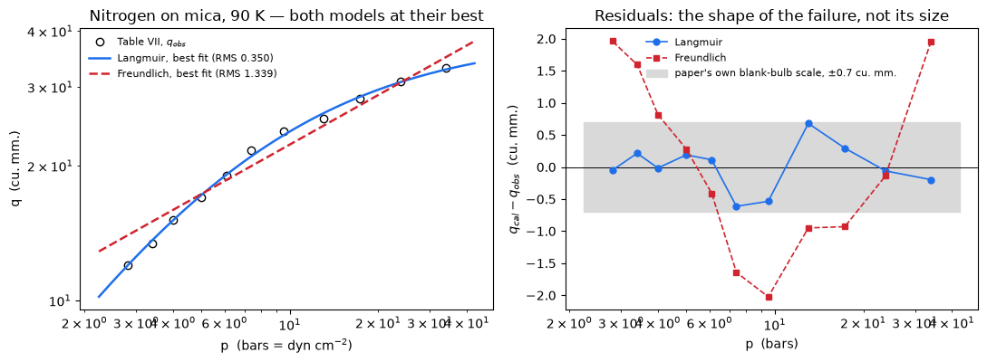
                                                         injected defect                        metric      before       after    effect                                                                                       note
      eq. (37) coefficient 25.2e15 -> 25.2e16 (the text layer's reading)                N0_max_rel_pct     1.62602     90.0566     MOVES                                                                                           
                                           same, propagated to the bound                      beta_max    0.857143     8.57143     MOVES               17 of 20 entries would exceed unity and the paper's conclusion would reverse
                              N 6.06e23 -> 6.60e23 (digit transposition)             chain_max_rel_pct    0.135917     8.95238     MOVES                                                                                           
                            R 83.2e6 -> 8.314e7 (SI-flavoured erg value)             chain_max_rel_pct    0.135917  0.00621641     MOVES                                                                                           
                         mica surface 5750 -> 5075 sq.cm (transposition)          s_inlier_max_dev_pct    0.482109     13.4206     MOVES                                                                                           
                                    methane/CO2 monolayer counts swapped                      beta_max    0.857143    0.885246     MOVES                                                                                           
                                                 eq. (38) sqrt(MT) -> MT         sigma_max_abs_rel_pct     3.76572     98.7926     MOVES                                                                                           
Table XXI sigma_liq inverted (a plausible misreading of 'relative life')                x_max_anywhere  0.00150348 9.87724e-05     MOVES                                                                                           
        Freundlich NOT refitted (the paper's own 8.4 p^0.417 everywhere)             disc_median_ratio     2.12107     29.4154     MOVES                         the contest gets EASIER for Langmuir, which is why the page refits
             Langmuir fitted by Langmuir's linearisation instead of on q             disc_median_ratio     2.12107     1.91368     MOVES            the transform reweights towards low pressure; this is why section 5 uses newton
                                  eq. (30): sign of sigma_1 in b flipped          sym_caseVI_minus_BET           0   0.0855595     MOVES                                                                                           
                   eq. (30): the 4 sigma_2^2 in c changed to 3 sigma_2^2       sym_collapse_c_residual           0     25.4074     MOVES                                                                                           
           1 % separation sampled on a 40-point log grid, not root-found               x_1pct_rootfind  0.00989933   0.0105194     MOVES                                                                                           
                                               eq. (15) taken as printed         t_half_eq15_corrected    0.109954           0     MOVES                                                          this IS the defect of section 6.7
                         eq. (14) marched with 200 steps instead of 1600 eq14_vs_eq15corrected_max_abs  0.00178013   0.0139974     MOVES                                                                                           
            half-coverage root-found on a 200-step march instead of 1600      t_half_march_vs_eq16_rel  0.00187536   0.0150845     MOVES the metric IS a discretisation error, so coarsening dt must scale it -- and it scales by 8
       Table IV: printed b = 58.3 used instead of the two-point solution        t4_two_route_b_rel_pct   0.0110162      1.3913     MOVES                                                                                           
                                    Table VII top row q_obs 33.0 -> 30.0                   t7_F_over_L     3.82349     2.60511     MOVES                                                                                           
                                  one Bulb A row dropped from Table VIII              n_obs_mismatches           0           1     MOVES                                      the 'Number of obs.' identity of section 4, recounted
                      Table XX beta 0.36 accepted rather than recomputed  order_breaks_recomputed_beta           0           1     MOVES                                                                                           
                               platinum area 312 -> 156 sq.cm (one face)             pt_N0_max_abs_dev           0        0.43     MOVES                                                                                           
                            Table XXII combined with the arithmetic mean        t22_multi_geom_max_pct     1.68121           4     MOVES                                                                                           
                      monolayer chain: cube root replaced by square root                mono_n_rel_pct    0.450533 2.58643e+09     MOVES                                                                                           
             separation read at the mean pressure instead of the maximum             departure_max_pct    0.160215   0.0394963     MOVES                monotonicity is what licenses the maximum; without it this is a sampled max
          eq. (22): the bare fraction theta_0 omitted from the inventory             sym_eq26_residual           0    0.860357     MOVES                                                                                           
                 1 % separation from the c -> infinity closed form 1/101               x_1pct_rootfind  0.00989933  0.00990099     MOVES                                                                                           
                                                 every b' scaled by 1.37          scatter_over_sep_min     12.1974     12.1974 -- no ---                STRUCTURAL: the ratio is scale-free in q, so a common factor cannot move it
                             sigma symbols renamed in the eq. (30) check           sym_eq30_c_residual           0           0 -- no ---                     STRUCTURAL: symbolic identity is invariant under renaming, and says so
                     Table VIII q_cal 84.8 -> 48.8 (digit transposition)            qcal_max_abs_cu_mm       0.434     36.3678     MOVES                                                                                           
                       Table IV b' repaired to 101.4 instead of reported               s_worst_dev_pct      1.3913    0.658762     MOVES                                                                                           
                      Table XX beta repaired to 0.46 instead of reported              beta_max_abs_dev         0.1           0     MOVES                                                                                           
                                            Table XXI sigma_liq inverted            t22_single_max_pct     2.26804      591616     MOVES                                                                                           
                                            Table XXI sigma_liq inverted                 p0_N2_90K_atm     3.77472    0.339724     MOVES                                                                                           
                                            Table XXI sigma_liq inverted           scatter_over_sep_t7     1104.38      99.385     MOVES                                                                                           
                                            Table XXI sigma_liq inverted          scatter_over_sep_min     12.1974      99.385     MOVES                             the STRUCTURAL row above cannot move this metric; this one can
        printed q_F column checked against 8.4 p^0.42 instead of p^0.417         qF_column_max_dev_pct     1.32475     1.99699     MOVES                                                                                           
                                    Table VII top row q_obs 33.0 -> 30.0                  t7_null_mean     19.4041     9.21401     MOVES                                                                                           
                                    Table VII top row q_obs 33.0 -> 30.0                    t7_null_kp     26.7732     14.1539     MOVES                                                                                           
                        Table VII optimum taken on the p/q linearisation          t7_graphical_penalty     1.06312     1.05644     MOVES                                                                                           
                  eq. (30): a = sigma_1 - 2 sigma_2 -> sigma_1 - sigma_2           sym_eq30_a_residual           0        1.25     MOVES                                                                                           
                                    eq. (30): b's 4 sigma_2 -> 3 sigma_2           sym_eq30_b_residual           0      1.5625     MOVES                                                                                           
                    eq. (30): c's 6 sigma_2 sigma_3 -> 5 sigma_2 sigma_3           sym_eq30_c_residual           0     3.51562     MOVES                                                                                           
              collapse claim 1 evaluated on b with the 3 sigma_3 dropped       sym_collapse_b_residual           0     16.3333     MOVES                                                                                           
                       collapse claim 2 evaluated with sigma_4 left free      sym_collapse2_c_residual           0      0.9375     MOVES                                                                                           
                 infinite ladder built with no distinguished first layer sym_ladder_infinite_minus_BET           0    0.322709     MOVES                                                                                           
                    ladder: the bare fraction dropped from the inventory  caseVI_series_vs_closed_form       1e-13    0.108108     MOVES                      'before' is the bound the gap is held to; the gap itself is round-off
                              ladder truncated at 5 layers instead of 20     caseVI_ladder_20layer_rel  0.00029315    0.169872     MOVES                                                                                           
         eq. (14) marched with a midpoint rule instead of implicit Euler               eq14_time_order    0.994844     2.00955     MOVES          the observed order is a property of the scheme and must move when the scheme does
                                               Table VII a 0.156 -> 0.15                slope_at_3bars    0.681199    0.689655     MOVES                                                                                           
                                               Table VII a 0.156 -> 0.15              slope_100_factor        3.32         3.2     MOVES                                                                                           
                                               Table VII a 0.156 -> 0.15               p_for_slope_020      25.641     26.6667     MOVES                                                                                           
                       c halved (sigma_1/sigma_2 from a different table)          x_1pct_two_route_rel 0.000167572 0.000335088     MOVES                                                                                           
                         the sampling grid refined from 40 to 400 points     x_1pct_sampling_error_pct     6.26395     1.35976     MOVES                                                                                           
           1 % separation sampled on a 40-point log grid, not root-found             p_1pct_over_p_max      1113.6     1183.35     MOVES                                                                                           
                                            Table XXI sigma_liq inverted                x_max_90K_only 0.000773605 1.33266e-13     MOVES                                                                                           
             separation read at the mean pressure instead of the maximum        departure_max_90K_only   0.0822576   0.0247703     MOVES                                                                                           
                                every 155 K row kept rather than dropped scatter_over_sep_min_90K_only     31.1144     12.1974     MOVES            this is the sensitivity itself: the metric IS the value with those rows dropped
                                            Table XXI sigma_liq inverted    x_max_155K_permanent_gases 1.17458e-06 3.79949e-19     MOVES                                                                                           
       Table VII's q replaced by Case VI's own curve reaching p/p0 = 0.3            t7_BET_free_over_L    0.999987 9.24535e-12     MOVES         the power check: the free contest CAN see multilayer adsorption when it is present
                             p0 margin computed on the 90 K entries only   p0_shrink_factor_for_parity      12.145     30.4035     MOVES                                                                                           
                                                 Table IV b 58.3 -> 57.5          t4_b_printed_dev_pct     1.40247   0.0110174     MOVES                                                                                           
                 newton tol and backward_tol loosened to 1e-3 on one fit         fit_two_route_max_rel       1e-09 1.00003e-07     MOVES                      'before' is the bound the gap is held to; the gap itself is round-off
                                    methane/CO2 monolayer counts swapped                 beta_headroom     1.16667     1.12963     MOVES                                                                                           
      eq. (37) coefficient 25.2e15 -> 25.2e16 (the text layer's reading)              beta_n_above_one           0          17     MOVES                                                                                           

62 of 64 injected defects move their metric. The 2 that do not are labelled STRUCTURAL above, are the ONLY rows so labelled, and are cited as evidence for nothing: a scale-free ratio cannot notice a common factor, and a symbolic identity cannot notice a renaming. Both metrics they name are separately covered by rows that DO move them.

7.3 Claims, coverage, and how CI checks them

Every number above that the page stands behind is registered once, with how it is checked (docs/claims-design.md): a value against the committed baseline within its stated relative tolerance, a bound against its stated limits on every run and every machine, an exact result by equality.

The bounds are the quantities whose size is not physics. The nine symbolic residuals are zero by construction (sympy simplifies them to 0) and are held at exactly 0. The 4000-layer numerical ladder against the BET closed form is floating-point summation error, held below \(10^{-13}\). fit_two_route_max_rel is the gap between two root-finders handed the same objective, set by their tolerances, held below \(10^{-9}\). The observed order of the implicit march is held between 0.9 and 1.1, because implicit Euler is first order.

Every claim has at least one break row from §7.2 that fails its own check, and the set of claims is asserted key-for-key against the set of metrics the break table aims at. Where a row moves its value by less than 5 %, the value’s tolerance is tightened below that move; every value on this page is identical to the last digit under three BLAS kernels, so a tight tolerance is admissible.

claims = Claims(PAGE)
# tolerances tightened below the move of the break row aimed at the value (every
# value here has zero spread across three BLAS kernels, so each is admissible)
RTOL = {"t7_BET_free_over_L": 1e-6, "t7_graphical_penalty": 1e-3, "slope_at_3bars": 2e-3, "beta_headroom": 5e-3,
        "slope_100_factor": 5e-3, "p_for_slope_020": 5e-3}
def value(k, **kw):
    claims.value(k, RES[k], rtol=RTOL.get(k, 0.05), **kw)

# transcription and the printed identity web
value("chain_max_rel_pct", unit="%")
claims.exact("n_obs_mismatches", int(RES["n_obs_mismatches"]),
             note="tables whose printed 'Number of obs.' differs from the rows transcribed")
value("qcal_max_abs_cu_mm", unit="cu.mm")
value("s_inlier_max_dev_pct", unit="%")
value("s_worst_dev_pct", unit="%")
value("N0_max_rel_pct", unit="%")
value("beta_max_abs_dev")
value("sigma_max_abs_rel_pct", unit="%")
value("t22_single_max_pct", unit="%")
value("t22_multi_geom_max_pct", unit="%")
claims.value("pt_N0_max_abs_dev", RES["pt_N0_max_abs_dev"], rtol=0.0, atol=5e-3,
             note="Table XXV N0 recomputed and rounded to the printed 0.01 against the "
                  "printed cells; 0 when every cell matches, at least 0.01 when one does not")
value("mono_n_rel_pct", unit="%")
value("t4_two_route_b_rel_pct", unit="%",
      note="two routes through printed, rounded constants; the gap is set by the printed digits")
value("t4_b_printed_dev_pct", unit="%")
# fit vs test: the discrimination and its nulls
value("disc_median_ratio")
value("t7_F_over_L")
value("t7_null_mean")
value("t7_null_kp")
value("t7_graphical_penalty")
value("qF_column_max_dev_pct", unit="%")
claims.bound("fit_two_route_max_rel", RES["fit_two_route_max_rel"], max=FIT_TWO_ROUTE_MAX,
             basis="tolerance",
             note="relative gap between newton (tol 1e-12) and brentq (xtol 1e-13) on the same "
                  "central-difference dS, worst over every fit; 9.4e-12 to 1.3e-11 on three BLAS "
                  "kernels in the locked environment")
# the out-of-sample bound
value("beta_max")
value("beta_headroom")
claims.exact("beta_n_above_one", int(RES["beta_n_above_one"]),
             margin=float((1.0 - g.beta_recomputed).abs().min()), min_margin=0.05,
             note="entries with recomputed beta >= 1; the margin is the smallest |beta - 1|")
claims.exact("order_breaks_recomputed_beta", int(RES["order_breaks_recomputed_beta"]),
             note="sets in which the order by recomputed beta differs from the order by b'")
# the symbolic family: zero by construction
for k in ("sym_eq26_residual", "sym_eq30_a_residual", "sym_eq30_b_residual",
          "sym_eq30_c_residual", "sym_collapse_b_residual", "sym_collapse_c_residual",
          "sym_collapse2_c_residual", "sym_caseVI_minus_BET", "sym_ladder_infinite_minus_BET"):
    claims.bound(k, RES[k], max=0.0, basis="identity",
                 note="sympy simplifies the difference to 0, evaluated at rational arguments")
claims.bound("caseVI_series_vs_closed_form", RES["caseVI_series_vs_closed_form"], max=1e-13,
             basis="chosen",
             note="4000-layer ladder summed term by term against the BET closed form at x = 0.2; "
                  "truncation is x^4000, so the gap is summation round-off (5.6e-16 measured)")
value("caseVI_ladder_20layer_rel", note="truncation error of the 20-layer ladder at x = 0.6")
# the rate equation
value("t_half_eq15_corrected")
value("eq14_vs_eq15corrected_max_abs", note="discretisation error, 1600 implicit steps")
claims.bound("eq14_time_order", RES["eq14_time_order"], min=0.9, max=1.1, basis="theory",
             note="observed order of implicit Euler over 200 to 1600 steps; first order")
value("t_half_march_vs_eq16_rel", note="discretisation error, 1600 implicit steps")
# the page's own result
for k in ("x_max_anywhere", "departure_max_pct", "scatter_over_sep_min",
          "scatter_over_sep_t7", "p0_N2_90K_atm", "x_1pct_rootfind"):
    value(k)
value("x_1pct_two_route_rel", note="the finite-c correction to the c -> infinity limit 1/101")
for k in ("x_1pct_sampling_error_pct", "p_1pct_over_p_max", "x_max_90K_only",
          "departure_max_90K_only", "scatter_over_sep_min_90K_only",
          "x_max_155K_permanent_gases", "t7_BET_free_over_L", "p0_shrink_factor_for_parity",
          # the log-log slope claim
          "slope_at_3bars", "slope_100_factor", "p_for_slope_020"):
    value(k)

# --- break rows: every row of section 7.2 that re-runs a computation ---------
# The two STRUCTURAL rows are designed non-movers and are not wired.
caught = set()
for name, target, before, after, effect, note in breaks:
    if not note.startswith("STRUCTURAL") and claims.breaks(name, target, after):
        caught.add(target)

targeted = set(bt.metric)
claimed = set(claims.metrics)
print("COVERAGE MAP, asserted key-for-key:")
print(f"  claimed but never broken : {sorted(claimed - targeted) or 'none'}")
print(f"  broken but not claimed   : {sorted(targeted - claimed) or 'none'}")
assert claimed == targeted, "coverage map and the claim registry disagree"
print(f"  {len(caught)} of {len(claimed)} claims have a break row "
      f"that FAILS the claim's own check")
not_reported = sorted(set(RES) - claimed)
print(f"\n{len(RES)} quantities computed; {len(claimed)} registered as claims. The other "
      f"{len(not_reported)} are printed on the page and checked in the prose audit below "
      f"where the markdown quotes them: counts, cardinalities, intermediates and alternative "
      f"readings.")
print("  not registered:", ", ".join(not_reported))

COVERAGE MAP, asserted key-for-key:
  claimed but never broken : none
  broken but not claimed   : none
  58 of 58 claims have a break row that FAILS the claim's own check

138 quantities computed; 58 registered as claims. The other 80 are printed on the page and checked in the prose audit below where the markdown quotes them: counts, cardinalities, intermediates and alternative readings.
  not registered: N0_cells, beta_cells, beta_entries, beta_max_corrected_hi, beta_max_corrected_lo, beta_n_above_one_textlayer, beta_n_exact, beta_textlayer_min_margin, blank_largest_negative_all, blank_largest_negative_glass, break_rows, break_rows_moving, c_t7, disc_min_null_kp, disc_min_null_mean, disc_n_langmuir_wins, disc_tables, disc_worst_ratio, eq14_march_steps, eq37_textlayer_factor, fit_two_route_count, glass_s_implied_median, hundred_bars_in_mmHg, mica_s_implied_median, mono_d_rel_pct, n_isotherm_points_A, n_isotherm_points_blank, order_breaks_printed_beta, p0_N2_90K_bars, p_for_slope_0684, printed_claims_rows, pt_cells, pt_foil_area, qcal_cells, qcal_median_abs_cu_mm, rp_entries, s_n_inliers, s_n_rows, s_second_worst_dev_pct, sigma_cells, sigma_mean_rel_pct, sigma_n_below, sigma_round_reproduces, sigma_trunc_reproduces, slope_at_100bars, slope_at_3bars_rel_pct, slope_at_t7_pmax, t13_rms_eq33, t13_rms_freundlich, t22_cells, t22_multi_arith_max_pct, t4_b_at_printed_a, t4_b_exact, t4_b_from_bprime, t5_t17_max_b_dev_pct, t7_BET_free_c, t7_BET_free_over_L_multilayer, t7_BET_free_vm, t7_L_second_route_rel, t7_a_optimal, t7_b_optimal, t7_p_max, t7_rms_optimal, t7_rms_printed, t9_ratio_all, t9_ratio_cut, t_half_closed_form_rootfind, t_half_closed_form_vs_eq16_rel, t_half_corrected_vs_eq16_rel, t_half_eq15_printed, t_half_eq16, t_half_march_order, t_half_march_rootfind, x_1pct_closed_form, x_1pct_sampled, x_entries_all, x_max_blank_bulb, x_max_eq31_bulbA_only, x_max_eq33_tables, x_rows_all

# ------------ prose audit: every number quoted in markdown, re-derived ------
# Numbers that are claims are checked by claims.says: within one unit of the last
# written place. Every one of them is identical to the last digit on three kernels.
SAYS = [
    ("3.82", "t7_F_over_L"), ("2.12", "disc_median_ratio"),
    ("1.1667", "beta_headroom"), ("0.857", "beta_max"), ("0", "beta_n_above_one"),
    ("below 1.6e-3", "x_max_anywhere"), ("0.160", "departure_max_pct"),
    ("12.2", "scatter_over_sep_min"), ("0.99999", "t7_BET_free_over_L"),
    ("12.14", "p0_shrink_factor_for_parity"), ("1104", "scatter_over_sep_t7"),
    ("0.434", "qcal_max_abs_cu_mm"), ("1.40", "t4_b_printed_dev_pct"),
    ("0.011", "t4_two_route_b_rel_pct"), ("0.136", "chain_max_rel_pct"),
    ("3.77", "sigma_max_abs_rel_pct"), ("0.6812", "slope_at_3bars"),
    ("25.64", "p_for_slope_020"), ("3.32", "slope_100_factor"),
    ("0.0098993", "x_1pct_rootfind"), ("1114", "p_1pct_over_p_max"),
    ("6.26", "x_1pct_sampling_error_pct"), ("1.063", "t7_graphical_penalty"),
    ("1.33", "qF_column_max_dev_pct"), ("3.775", "p0_N2_90K_atm"),
    ("1.78e-3", "eq14_vs_eq15corrected_max_abs"), ("0.995", "eq14_time_order"),
    ("1.875e-3", "t_half_march_vs_eq16_rel"), ("1.391", "s_worst_dev_pct"),
    ("0.451", "mono_n_rel_pct"), ("2.27", "t22_single_max_pct"),
    ("below 1e-9", "fit_two_route_max_rel"), ("below 1e-13", "caseVI_series_vs_closed_form"),
]
for lit, k in SAYS:
    claims.says(lit, k)

# Numbers that are not claims: counts compared exactly, the rest relative.
def close(name, quoted, key, tol=5e-3):
    got = RES[key]
    ok = abs(got - quoted) <= tol * max(1.0, abs(quoted))
    if not ok:
        raise AssertionError(f"PROSE DRIFT on {name}: markdown says {quoted}, cells give {got}")
    return True

audit = [
    ("tables where Langmuir wins", 13, "disc_n_langmuir_wins", 0),
    ("tables compared", 14, "disc_tables", 0),
    ("entries above unity under the text layer's 25.2e16", 17,
     "beta_n_above_one_textlayer", 0),
    ("beta entries", 20, "beta_entries", 0),
    ("separation-table entries", 18, "rp_entries", 0),
    ("table/gas/bulb entries with a p/p0", 30, "x_entries_all", 0),
    ("q_cal cells", 101, "qcal_cells", 0),
    ("eq. (37) text-layer factor", 10.0, "eq37_textlayer_factor", 1e-6),
    ("sigma printed below computed", 18, "sigma_n_below", 0),
    ("sigma cells", 21, "sigma_cells", 0),
    ("beta cells exact", 22, "beta_n_exact", 0),
    ("beta cells", 23, "beta_cells", 0),
    ("break rows", 64, "break_rows", 0),
    ("break rows that move", 62, "break_rows_moving", 0),
    ("fits done", 29, "fit_two_route_count", 0),
    ("implied mica area", 5747.4, "mica_s_implied_median", 1e-4),
    ("second b-prime outlier", 0.659, "s_second_worst_dev_pct", 1e-2),
    ("printed-claims rows", 36, "printed_claims_rows", 0),
]
for name, quoted, key, tol in audit:
    close(name, quoted, key, tol)
print(f"prose audit: {len(SAYS)} literals checked against their claims with claims.says, "
      f"{len(audit)} other numbers re-derived and matched. This cell RAISES on any drift "
      f"between the markdown and the output.\n")
_kinds = {kd: [k for k, c in claims.metrics.items() if c["kind"] == kd]
          for kd in ("value", "bound", "exact")}
print(f"{len(claims.metrics)} claims: {len(_kinds['value'])} values, "
      f"{len(_kinds['bound'])} bounds, {len(_kinds['exact'])} exact.\n")
payload = claims.report()

prose audit: 33 literals checked against their claims with claims.says, 18 other numbers re-derived and matched. This cell RAISES on any drift between the markdown and the output.

58 claims: 43 values, 12 bounds, 3 exact.

Claims for J1.1-langmuir-isotherm:
  chain_max_rel_pct             = 0.13592          value  rtol 0.05
  n_obs_mismatches              = 0                exact  exact
  qcal_max_abs_cu_mm            = 0.434            value  rtol 0.05
  s_inlier_max_dev_pct          = 0.48211          value  rtol 0.05
  s_worst_dev_pct               = 1.3913           value  rtol 0.05
  N0_max_rel_pct                = 1.626            value  rtol 0.05
  beta_max_abs_dev              = 0.1              value  rtol 0.05
  sigma_max_abs_rel_pct         = 3.7657           value  rtol 0.05
  t22_single_max_pct            = 2.268            value  rtol 0.05
  t22_multi_geom_max_pct        = 1.6812           value  rtol 0.05
  pt_N0_max_abs_dev             = 0                value  rtol 0, atol 0.005
  mono_n_rel_pct                = 0.45053          value  rtol 0.05
  t4_two_route_b_rel_pct        = 0.011016         value  rtol 0.05
  t4_b_printed_dev_pct          = 1.4025           value  rtol 0.05
  disc_median_ratio             = 2.1211           value  rtol 0.05
  t7_F_over_L                   = 3.8235           value  rtol 0.05
  t7_null_mean                  = 19.404           value  rtol 0.05
  t7_null_kp                    = 26.773           value  rtol 0.05
  t7_graphical_penalty          = 1.0631           value  rtol 0.001
  qF_column_max_dev_pct         = 1.3248           value  rtol 0.05
  fit_two_route_max_rel         = (here 9.4e-12)   bound  bound <= 1e-09 [tolerance]
  beta_max                      = 0.85714          value  rtol 0.05
  beta_headroom                 = 1.1667           value  rtol 0.005
  beta_n_above_one              = 0                exact  exact, margin 0.143
  order_breaks_recomputed_beta  = 0                exact  exact
  sym_eq26_residual             = (here 0.0e+00)   bound  bound <= 0 [identity]
  sym_eq30_a_residual           = (here 0.0e+00)   bound  bound <= 0 [identity]
  sym_eq30_b_residual           = (here 0.0e+00)   bound  bound <= 0 [identity]
  sym_eq30_c_residual           = (here 0.0e+00)   bound  bound <= 0 [identity]
  sym_collapse_b_residual       = (here 0.0e+00)   bound  bound <= 0 [identity]
  sym_collapse_c_residual       = (here 0.0e+00)   bound  bound <= 0 [identity]
  sym_collapse2_c_residual      = (here 0.0e+00)   bound  bound <= 0 [identity]
  sym_caseVI_minus_BET          = (here 0.0e+00)   bound  bound <= 0 [identity]
  sym_ladder_infinite_minus_BET = (here 0.0e+00)   bound  bound <= 0 [identity]
  caseVI_series_vs_closed_form  = (here 5.6e-16)   bound  bound <= 1e-13 [chosen]
  caseVI_ladder_20layer_rel     = 0.00029315       value  rtol 0.05
  t_half_eq15_corrected         = 0.10995          value  rtol 0.05
  eq14_vs_eq15corrected_max_abs = 0.0017801        value  rtol 0.05
  eq14_time_order               = (here 9.9e-01)   bound  bound [0.9, 1.1] [theory]
  t_half_march_vs_eq16_rel      = 0.0018754        value  rtol 0.05
  x_max_anywhere                = 0.0015035        value  rtol 0.05
  departure_max_pct             = 0.16022          value  rtol 0.05
  scatter_over_sep_min          = 12.197           value  rtol 0.05
  scatter_over_sep_t7           = 1104.4           value  rtol 0.05
  p0_N2_90K_atm                 = 3.7747           value  rtol 0.05
  x_1pct_rootfind               = 0.0098993        value  rtol 0.05
  x_1pct_two_route_rel          = 0.00016757       value  rtol 0.05
  x_1pct_sampling_error_pct     = 6.2639           value  rtol 0.05
  p_1pct_over_p_max             = 1113.6           value  rtol 0.05
  x_max_90K_only                = 0.00077361       value  rtol 0.05
  departure_max_90K_only        = 0.082258         value  rtol 0.05
  scatter_over_sep_min_90K_only = 31.114           value  rtol 0.05
  x_max_155K_permanent_gases    = 1.1746e-06       value  rtol 0.05
  t7_BET_free_over_L            = 0.99999          value  rtol 1e-06
  p0_shrink_factor_for_parity   = 12.145           value  rtol 0.05
  slope_at_3bars                = 0.6812           value  rtol 0.002
  slope_100_factor              = 3.32             value  rtol 0.005
  p_for_slope_020               = 25.641           value  rtol 0.005

8. What pymrm adds

To Langmuir’s isotherm, nothing. Eqs. (9), (26), (29), (31) and (33) are closed forms in one variable. There is no grid on this page, no time step in space, no boundary condition and no transport, and most of the notebook would run with pymrm uninstalled — the same honest answer A1.6, A1.1 and J1.3 give. newton and NumJac do three specific jobs, and each was chosen because the cheap alternative is wrong, not slow.

(1) A fit that shares no algebra with the paper’s fit. Langmuir drew a line through \(p/q\) against \(p\). That is linear least squares on a transformed variable, and the transform is not innocent: it reweights the residuals towards the low-pressure points, where \(q\) is small and \(p/q\) is most sensitive. Profiling the amplitude out and root-finding the remaining stationarity condition on \(q\) itself is a different computation, and the break table carries the row that shows it matters — fitting by his linearisation instead moves the Freundlich-versus-Langmuir ratio, which is the page’s discrimination metric. It also lets Freundlich be beaten at its best rather than at Langmuir’s rendering of it, which is the only version of that contest worth reporting.

(2) The rate equation integrated instead of quoted. Eq. (15) is printed wrongly. The way to establish that without asserting it is to integrate eq. (14) — which is what march_eq14 does, with a newton-solved implicit step — and see which branch the march reaches. It reaches the corrected one to \(1.8\times10^{-3}\) at 1600 steps, converging at first order in \(\Delta t\) (the one axis that carries error here), and it cannot reach the printed one at all, because the printed one puts \(t = -\infty\) at the start of the integration. That is a proof rather than a reading of the glyph.

(3) Root-finds where a sweep would have been wrong. The relative pressure at which Case VI departs from Case I by 1 % is root-found; reading it off a 40-point log grid gives a value 6.3 % out, and it is quoted in the same sentence as the number it is compared with. The pressures corresponding to the printed log-log exponents are root-found for the same reason.

(4) And the thing that is not pymrm at all, and is the most useful output on the page. Langmuir’s Case VI, eqs. (29) and (30), is the BET isotherm. That needed sympy and a change of variables the paper itself supplies through eq. (39), and it converts the paper’s central conclusion from “the isotherm shows the film is one molecule thick” into “the isotherm could not have shown anything of the kind, and the film being one molecule thick is what \(\beta\) shows”. The separation between his two theories, over his entire data set, is at most 0.16 %, against scatter 12 to 1100 times larger.

What this page does not do that a reader might want. It does not fit eq. (29) to Langmuir’s data. That would be meaningless: at \(p/p_0 < 10^{-3}\) the parameter \(c\) is not identifiable, and any fit would return the Case I answer with an arbitrary \(c\). Saying so is the finding.

9. Reuse

What you can take from here

• The isotherm itself, in either parameterisation: \(q = abp/(1+ap)\) with \(a\) in reciprocal bars, or \(\theta = Kp/(1+Kp)\). If you need it inside a reactor or a breakthrough model, J1.5 (LDF breakthrough) is the page with the transport; this one has none.
• The identity chain \(b \to b' \to N_0 \to \beta\). It is the cheapest self-check that exists for any adsorption dataset reported as a monolayer capacity: convert to molecules per unit area and divide by a close-packing count from the liquid density. If \(\beta > 1\) your surface area is wrong, your isotherm is not Langmuir, or both.
• The discrimination protocol. Refit both rivals, count the parameters, print a zero-parameter and a one-parameter null beside the ratio, and check whether the residuals sweep. A power law forced through a saturating curve leaves a signature you can see (§6.6’s right-hand panel) long before the RMS tells you.
• The relative-pressure check, which is the transferable lesson. Before claiming that data support a monolayer model over a multilayer one, compute \(p/p_0\) and evaluate how far apart the two models actually are there. On this paper the answer is 0.16 % at best, against 1–3 % scatter.

What you must not take from here

• The \(q_\mathrm{cal}\) agreement is a fit. It is stated as one in the notebook, in meta.yaml, in models_entry.yaml, in README.md and on the case yaml. It is never reported as an agreement metric. If you see it quoted as evidence for the Langmuir model, that is this page being misread.
• Tier 5, and only one column of it is measurement. \(q_\mathrm{obs}\) is measured; \(a\), \(b\), \(b'\), \(\sigma\), \(N_0\), \(\beta\) and Tables XXI, XXII, XXV are all derived by Langmuir from those measurements. Reproducing them is reproduction, never validation.
• The mica numbers are uncorrected. The paper says 10–30 % too high, and no correction is applied anywhere on this page.
• Four printed defects, reported and none repaired — §6.7 eq. (15)’s logarithm; §6.2/§6.3 Table IV’s \(b = 58.3\); §6.3/§6.5 Table XX’s \(\beta = 0.36\) for methane on glass; §6.10 the pair “(100 bars) … 0.20”. Where a correction is stated it is labelled an inference.
• And, kept separate from them, one reporting convention. The \(\sigma\) column of Tables XVIII–XX runs low against eq. (38): 18 of 21 printed values lie below the computed one, worst 3.77 %. That is a real and non-random pattern, but it is not an error against Langmuir, and §6.3 shows why — the three worst rows are exactly the rows he prints to one or two significant figures, and truncating at each cell’s own printed granularity reproduces more cells than rounding does. He discarded figures; he did not miscompute them. Filing it as a fifth defect would overstate it.
• Nothing here is about platinum. Journal pages 1393–1401 are irreversible chemisorption with no isotherm, and Tables XXIII and XXIV were deliberately not transcribed.

Origins cited but not consulted

Freundlich, H., Kapillarchemie, Leipzig (1909) — the rival isotherm, read only through Langmuir’s own restatement of it on journal page 1375 and through the \(q_F\) column of Table VII. Eucken (1914); Bakker (1915); Haber (1914); Knudsen, Ann. Physik 31, 205 (1910), the thermal-effusion correction; Meyer’s Kinetic Theory of Gases (1899), the source of eq. (1); and Langmuir’s own Parts I and II (This Journal 38, 2221 (1916) and 39, 1848 (1917)), which carry the monomolecular-film evidence this paper leans on. None is on disk and none was consulted. Nothing on this page derives from any of them.

Brunauer, Emmett & Teller (1938) is on disk and is the subject of J1.3. The only thing taken from it here is the form of the BET isotherm, which J1.3 documents as its eqs. (26)/(28); no dataset of J1.3 is loaded and no number of J1.3 is retyped, and the identity of §6.8 is verified against Langmuir’s eq. (30) rather than against anything BET print. That the two theories are related is not this page’s discovery and the 1938 paper says so itself — its Section II is headed “Generalization of Langmuir’s Theory to Multimolecular Adsorption”, read here on a 300 ppi crop of journal page 311. What is new is that Langmuir’s own Case VI closed form already is that generalisation, and that his data lie where it cannot be told apart from Case I.

And one thing this page checked for somebody else

Rawlings & Ekerdt, Chemical Reactor Analysis and Design Fundamentals (2nd edn), book page 443, state that the Danckwerts boundary conditions “were derived at least 45 years prior to Danckwerts in a classic paper by Langmuir [22]”. That paper is not this one. Their reference [22] is Langmuir, I., “The velocity of reactions in gases moving through heated vessels and the effect of convection and diffusion”, J. Am. Chem. Soc. 30(11), 1742–1754 (1908) — read from their own bibliography, and 1953 − 1908 = 45 exactly. The 1918 paper on disk contains no flow, no convection and no boundary condition of any kind: the words “convection” and “flow” do not occur in its forty-three pages, “diffusion” occurs three times and never in a transport equation, and every apparatus in it is a sealed static bulb. The claim bears on A2.1/A2.2 and cannot be settled from this file; settling it needs JACS 30(11) 1742, which is not on disk. Recorded on the case yaml as an acquisition target. A2.1 and A2.2 were not touched.