# Bootstrap: the pymrm this page was checked with, and the gallery files it was
# published with. Works in a checkout, in CI and on a fresh Colab VM.
GALLERY_REF = "gallery-2026.11.10.3"  # replaced by the release tag at publication
PYMRM = ">=3.3.0,<4"  # equals meta.yaml pymrm_min_version, up to the next major
PAGE = "G1.8-trickle-bed-partial-wetting"  # equals the page directory

import os, sys, urllib.request
from pathlib import Path
_shared = next((p / "shared" for p in (Path.cwd(), *Path.cwd().parents)
                if (p / "shared" / "gallery_bootstrap.py").is_file()), None)
if _shared is None:
    _shared = (Path(os.environ.get("XDG_CACHE_HOME") or Path.home() / ".cache")
               / "pymrm-gallery" / GALLERY_REF)
    _shared.mkdir(parents=True, exist_ok=True)
    urllib.request.urlretrieve(
        "https://raw.githubusercontent.com/computational-chemical-engineering/"
        f"pymrm-gallery/{GALLERY_REF}/shared/gallery_bootstrap.py",
        _shared / "gallery_bootstrap.py")
sys.path.insert(0, str(_shared))
sys.modules.pop("gallery_bootstrap", None)
from gallery_bootstrap import setup
setup(PAGE, PYMRM, GALLERY_REF); # the semicolon stops the cell echoing the pathTrickle-bed reactor with partial catalyst wetting
sec:G
struct:S8
tier:T1
data:tier6
phase:gas-liquid-solid
A partially wetted pellet fed from two sides at once, and a printed figure whose legend is off by one row: reconstructed, quantified, and shown both ways.
Trickle-bed reactor with partial catalyst wetting
Catalog ID: G1.8 · Structures: S8 (diffusion–reaction in a particle with mixed external resistances) · Tier: T1
In a trickle bed the liquid does not cover the packing. Part of every pellet is wetted and part is dry, and a volatile reactant can reach the dry part straight from the gas, bypassing the gas–liquid film and the liquid–solid film that stand between it and the wetted part. Partial wetting is then not a penalty at all: it is a shortcut, and Herskowitz & Smith’s Figure 6 measures how large a one.
This page reproduces that figure from the paper’s own equations, and in doing so reports two printed defects in the source: a cross-reference to the wrong table, and a legend whose rows are misaligned by one against the curves they label. The second one is why the figure looks unreproducible until it is fixed.
This is not experimental validation. Figure 6 contains no data: the four lines on it are the authors’ own computed model output. Reproducing them tests a transcription and a chain of algebra. The page is tier 6 and says so everywhere.
import numpy as np
import pandas as pd
import matplotlib.pyplot as plt
from scipy.sparse import eye_array
from scipy.sparse.linalg import splu
from scipy.special import i0e, i1e
from IPython.display import Markdown, display

from pymrm import newton
from gallery_utils import load_data, load_meta, cite_data, Claims
from model import (Closures, PAPER, eta_sphere, chi_table1, chi_collapsed,
                   reconstruct_L, alpha_gs_for, WettedSphere)

plt.rcParams.update({"figure.dpi": 110, "axes.grid": True, "grid.alpha": 0.3})
claims = Claims(PAGE.split("-")[0])


# Deviation convention, used EVERYWHERE on this page and nowhere reversed:
#     dev = (model - figure) / figure
def dev(model, figure):
    return (np.asarray(model, float) - np.asarray(figure, float)) / np.asarray(figure, float)


COL = ["#1f77b4", "#d62728", "#2ca02c", "#9467bd"]   # one colour per drawn curve
Background
Herskowitz & Smith (1983) is a review of trickle-bed reactors, and its partial-wetting section is the piece the gallery wants. The physical picture:
- The external surface of a catalyst pellet is split into a wetted fraction \(f_e\) (covered by flowing liquid) and a dry fraction \(1-f_e\) (covered at most by a stagnant film, and in contact with the gas).
- A limiting reactant that is non-volatile can only arrive through the liquid. Partial wetting then costs external area, and the effect on the overall effectiveness factor is modest; the paper says so explicitly for \(0.6 < f_e < 1\).
- A limiting reactant that is volatile can arrive at the dry surface directly from the gas. The gas-side external resistance is normally far smaller than the gas–liquid plus liquid–solid resistance in series, so the dry patch is the better supplied one. Partial wetting then raises the overall effectiveness factor, and the more strongly the more diffusion-limited the pellet is.
Figure 6 quantifies the second case in the limit where the gas-side resistance is negligible altogether. Its ordinate is
\[ \chi = \frac{\eta_o - \eta_o(f_e=1)}{\eta_o(f_e=1)} \tag{19} \]
the fractional gain in overall effectiveness factor relative to a fully wetted pellet, plotted against the Thiele modulus \(\phi\) for four liquid mass velocities \(L_m\). Everything on that figure is positive and rises with \(\phi\): at the right edge of the figure the top curve’s gain is more than tenfold.
That is the practical warning the section is built around. If you measure a rate in a trickle bed and vary the liquid flow to test for mass-transfer limitation, the two mechanisms move in opposite directions: lowering \(L_m\) dries more surface (helping a volatile reactant) while starving the wetted surface (hurting it). The paper’s own words: doing so “may lead to pitfalls.”
The gallery’s structural claim
S8 here is the classical pellet problem of B1.1 with a mixed external boundary condition: the same interior equation, two different Robin conditions on two parts of one surface. The paper handles that by superposition of two whole-surface problems (its Eq. 6, from Ramachandran & Smith 1979), which is an approximation, and the page is careful to say that nothing here tests it.
The published model
Read from a 600 dpi render of the paper (the PDF text layer mangles every equation on these pages). Page numbers are journal pages.
The particle problem (page 4). For an isothermal, irreversible, \(m\)-th order reaction in a porous particle,
\[ \nabla^2 C - \phi^2 C^m = 0, \qquad \phi = \frac{V_p}{S_x}\sqrt{\frac{\rho_p k_v C_L^{m-1}}{D_e}}, \qquad C = C_i/C_L \tag{3} \]
with \(\nabla\) non-dimensionalised on the characteristic length \(V_p/S_x\), for a sphere \(R/3\). The external surface is divided into a wetted part \(S_w\) and a “dry” part \(S_D\), carrying different Robin conditions:
\[ \frac{\partial C}{\partial n} = \alpha_{gLs}\,(C^*_L - C) \ \ \text{on } S_w, \qquad \frac{\partial C}{\partial n} = \alpha_{gs}\,(1 - C) \ \ \text{on } S_D \tag{4a, 4b} \]
with \(C^*_L = C_{L,b}/C_L\), and \(\alpha_{gLs}\) the gas–liquid and liquid–solid resistances in series (Eq. 4d). The overall effectiveness factor is the volume average of the local rate, \(\eta_o = V_p^{-1}\int_{V_p} C^m\,dV\) (Eq. 2a).
Table 1, sphere row (page 4). For \(m = 1\), superposing a fully wetted and a fully dry particle in the proportion \(f_e : 1-f_e\) (Eq. 6) gives a closed form:
\[ \eta_o = \frac{f_e C^*_L} {\dfrac{\phi^2}{\alpha_{gLs}} + \dfrac{3\phi^2}{3\phi\coth 3\phi - 1}} + \frac{1 - f_e} {\dfrac{\phi^2}{\alpha_{gs}} + \dfrac{3\phi^2}{3\phi\coth 3\phi - 1}} \tag{Table 1} \]
The two closures Figure 6 uses (page 8):
\[ f_e = 0.77\,L_m^{0.1} \tag{20} \]
\[ \frac{1}{\alpha_{gLs}} = \frac{1}{1.05\,L_m^{0.3}} + \frac{1}{6.91\,L_m^{0.6}} \tag{21} \]
Eq. 21 is stated to be Eq. 4d with the Goto & Smith (1975) and Specchia et al. (1978) correlations substituted at the operating conditions printed in the figure caption. The figure’s own two stated closing assumptions are \(\alpha_{gs} \to \infty\) (“very large”) and \(C^*_L = 1.0\).
Printed defect 1: the wrong table is cited
Page 8 reads: “The overall effectiveness factor is calculated from the approximate solution for a spherical particle given in Table 2.” Table 2 holds the pressure-drop constants \(\beta\) and \(\gamma\). The spherical solution is the third row of Table 1, page 4. Checked on 600 dpi renders of both pages and against the paper’s notation list. This is a typographic slip with no effect on any number; it is recorded because a reader following the citation finds nothing usable.
The chain collapses
With \(\alpha_{gs}\to\infty\) the dry term loses its external resistance and becomes the plain sphere effectiveness factor \(\eta_s(\phi) = (3\phi\coth 3\phi - 1)/(3\phi^2)\); with \(C^*_L = 1\) the wetted term is exactly \(\eta_o(f_e=1)\). So Table 1 reads \(\eta_o = f_e\,\eta_o(f_e{=}1) + (1-f_e)\,\eta_s\), and Eq. 19 collapses to
\[ \chi = (1 - f_e)\,\eta_s(\phi)\,\frac{\phi^2}{\alpha_{gLs}} \tag{collapse} \]
a product of one factor per assumption: how much surface is dry, how deep the pellet is, and how large the resistance the dry patch bypasses. This is used below as a reading aid and a root-finding target; it is an algebraic identity, not evidence, and the page labels it as such.
The paper’s algebra, transcribed
model.py holds one function per printed equation: Closures (Eqs. 20 and 21, with the printed constants as defaults), eta_sphere, eta_o_table1 and chi_table1 (Table 1’s sphere row and Eq. 19), and chi_collapsed. They contain no fitted quantity.
# --- check the transcription of Eq. 20 against the numbers printed IN the figure
L_LEGEND = np.array([0.50, 1.0, 2.0, 7.0])
FE_PRINTED = np.array([0.72, 0.77, 0.83, 0.94])
fe_eq20 = PAPER.f_e(L_LEGEND)

lines = ["Eq. 20 against the f_e column printed inside Figure 6",
         "  L_m    printed   Eq. 20    rounded   match"]
for L, p, c in zip(L_LEGEND, FE_PRINTED, fe_eq20):
    lines.append(f"  {L:<6.2f} {p:<9.2f} {c:<9.4f} {round(c, 2):<9.2f} "
                 f"{'OK' if abs(round(c, 2) - p) < 5e-3 else 'MISMATCH'}")

# and the collapse, as the identity it is
_phi = np.logspace(0, 1.7, 25)
IDENTITY = float(np.max(np.abs(chi_collapsed(_phi, 2.0) / chi_table1(_phi, 2.0) - 1.0)))
lines.append(f"\ncollapse vs full Table 1 chain (algebraic identity): "
             f"max rel diff (here {IDENTITY:.1e})")
print("\n".join(lines))
Eq. 20 against the f_e column printed inside Figure 6
L_m printed Eq. 20 rounded match
0.50 0.72 0.7184 0.72 OK
1.00 0.77 0.7700 0.77 OK
2.00 0.83 0.8253 0.83 OK
7.00 0.94 0.9354 0.94 OK
collapse vs full Table 1 chain (algebraic identity): max rel diff (here 1.3e-15)Parameters and assumptions
Everything numeric on this page traces to one of three places, and the page never mixes them:
| source | what it is | |
|---|---|---|
| \(f_e\), \(\alpha_{gLs}\) | Eqs. 20, 21, page 8 | printed closures, transcribed from a 600 dpi render |
| \(\eta_o\) | Table 1 sphere row, page 4 | printed closed form, transcribed the same way |
| \(\alpha_{gs}\to\infty\), \(C^*_L = 1\) | figure caption + page 8 text | stated assumptions |
| the four curve positions | digitised, data/ |
the only extracted quantity |
| \(L_m \approx 10\) for the fourth curve | reconstructed on this page | labelled reconstruction, see below |
The caption’s conditions (\(Sc_L = 100\), \(d_p = 1.5\times10^{-3}\) m, \(\varepsilon_p = 0.5\), \(\varepsilon_B = 0.4\), \(\tau = 2\), \(\mu_L = 8\times10^{-4}\) kg/(m·s)) are what produced the constants in Eq. 21. They do not enter this page again: Eq. 21 already contains them, and re-deriving it would mean transcribing two further correlations from papers not on disk. That is a deliberate limit and it is listed as a blind spot at the end.
Assumptions inherited, all of them the paper’s:
- First order, \(m = 1\): Table 1 exists only for \(m=1\).
- Isothermal. The paper separately argues \(T_s - T_f < 0.5\) K under the relevant conditions.
- Eq. 6 superposition: the partially wetted particle is a weighted average of two whole-surface particles. This is the paper’s approximation to a genuinely multi-dimensional boundary-value problem, and nothing on this page tests it.
- \(\alpha_{gs}\) literally infinite. Section “Validation” measures how much that matters: quite a lot.
The data
One dataset, and it is not measurements. Figure 6 carries four drawn lines and no markers whatsoever; the lines are the authors’ own model output. The CSV holds, per drawn curve, a straight line fitted to it in \((\log\phi, \log\chi)\): its slope, its position expressed as \(\chi\) at \(\phi = 10\), the traced \(\phi\) range, and the rms residual of the fit.
Three consequences the page holds to throughout:
- Tier 6, never “validated”. Reproducing a computed curve tests transcription and algebra. It cannot test the model against nature.
- Away from the fit’s own parametrisation there are no raw points. Any deviation quoted at a \(\phi\) other than through these four fitted lines is model against a fitted line, and is labelled that way.
- The reduction to a straight line is itself lossy, quantified in Results, where the model’s own best straight-line fit turns out to have an rms of the same order as the digitisation’s.
The maintainer reviewed Figure 6 in a private decision artifact on 2026-08-02 and endorsed the conclusion drawn from these four fits. What was reviewed was the reading (the figure alongside the reconstruction below), not a marker-by-marker audit, which Figure 6 does not admit. That review is what licenses the use of these rows; the numbers in the CSV are unchanged from the 2026-07-29 extraction.
The sidecar also records the abscissa calibrations behind the slope analysis of Results: the one this CSV was traced with, three other readings of the same four labelled \(\phi\) verticals, and the result of an independent re-digitisation made during the 2026-08-02 verification pass. They are read from the sidecar below, not recomputed: the figure image is not part of the gallery.
fig6 = load_data("herskowitz-smith-1983-fig6.csv", page=PAGE)
meta6 = load_meta("herskowitz-smith-1983-fig6.csv", page=PAGE)
print(cite_data(meta6))
print()
print(fig6.to_string(index=False))
print()
print("estimated error:", meta6["acquisition"]["estimated_error"])

CHI10 = fig6["chi_at_phi_10"].to_numpy()          # position of each drawn curve
SLOPE = fig6["slope_dlogchi_dlogphi"].to_numpy()  # its fitted log-log slope
PHI_LO = float(fig6["phi_min"].iloc[0])
PHI_HI = float(fig6["phi_max"].iloc[0])
RMS_FIT = fig6["fit_rms_decades"].to_numpy()
CHI_ERR_PCT = 100.0 * (10.0 ** RMS_FIT - 1.0)      # the fit rms, expressed in chi

CAL = meta6["abscissa_calibrations"]
CAL_CSV = float(meta6["acquisition"]["phi_px_per_decade"])   # this CSV's calibration
CAL_ALT = {k: float(v) for k, v in CAL["alternatives_px_per_decade"].items()}
INDEP = CAL["independent_retrace"]


def line_chi(phi, i, slope=SLOPE):
    """The i-th DIGITISED FITTED LINE evaluated at phi. Not raw pixels."""
    return CHI10[i] * (np.asarray(phi, float) / 10.0) ** slope[i]
Herskowitz, M.; Smith, J. M. (1983) — AIChE Journal 29(1) 1-18 — doi:10.1002/aic.690290102 — digitised from Figure 6, journal page 8 (= PDF page 8)
L_m_kg_m2_s f_e slope_dlogchi_dlogphi chi_at_phi_10 phi_min phi_max fit_rms_decades
0.5 0.72 1.1051 3.7515 1.07 45.5 0.0290
1.0 0.77 1.0976 1.4412 1.07 45.5 0.0282
2.0 0.83 1.1122 0.3543 1.07 45.5 0.0289
7.0 0.94 1.1311 0.1429 1.07 45.5 0.0235
estimated error: fit rms 0.023 to 0.029 decades, i.e. about 6 % in chiPyMRM implementation
The closed form above is an answer, not a model. The model is Eq. 3 with the Robin conditions 4a/4b, and that is what pymrm solves: one spherical finite-volume BVP per external condition, combined by the paper’s Eq. 6 (WettedSphere in model.py).
Two conventions carry all the risk here, and both are about the length scale:
- The paper’s \(\phi\) is built on \(V_p/S_x = R/3\), so on a grid \(u = r/R\) the interior equation is \(\nabla_u^2 C = (3\phi)^2 C^m\).
- The paper’s \(\partial C/\partial n\) in Eqs. 4a/4b is also per unit \(V_p/S_x\), so \(\partial C/\partial n = \tfrac13\,\partial C/\partial u\) and the Robin condition in grid units is \(\partial C/\partial u + 3\alpha C = 3\alpha C^*\).
Both factors of 3 are asserted, not printed, so both are broken on purpose in Validation to show the check notices.
House conventions followed:
- Outward normal. At \(u=0\) the outward normal points into the pellet, so symmetry is
{a:1, b:0, d:0}. At \(u=1\) the Robin condition \(\partial C/\partial n = \alpha(C^*-C)\) becomes \(a\,\partial C/\partial u + bC = d\) witha=1, b=3α, d=3αC*; the \(\alpha\to\infty\) limit is the Dirichlet{a:0, b:1, d:C*}. - Constant operators assembled once, cached per boundary condition, never inside Newton.
- Layout
(n_u, 1): spatial axis first, single field last, soNumJacbuilds the diagonal Jacobian of the pointwise source. nu=2inconstruct_divis the spherical geometry factor.- Newton with
tol=1e-10, above the round-off floor of the unknowns, andbounds=(0, None), because \(C^m\) is undefined below zero for a non-integer order.solveraises whennewtondoes not report convergence, so no number on this page comes from a failed solve. - Every solve is a direct Newton solve from a flat guess. At \(m = 1\) the problem is linear, and for \(m > 1\) the rate increases with \(C\), so the pellet problem has one solution: there is no branch for
pymrm.continuationto follow and no hard start forpymrm.pseudo_transientto relax, and neither is used.
sph = WettedSphere(n_u=800)
_y = sph.solve(10.0, float(PAPER.alpha_gLs(2.0)))
_r = sph.last_result
print(f"pymrm sphere, n_u = {sph.n_u}: eta = {sph.eta(_y):.8f}, newton status {_r.status} "
      f"(converged), backward error (here {_r.backward_error:.1e})")
pymrm sphere, n_u = 800: eta = 0.01028277, newton status 0 (converged), backward error (here 3.8e-12)The pymrm solve against Table 1
The finite-volume route and Table 1’s closed form share nothing (one discretises the BVP, the other is a formula), so this comparison can fail, and Validation shows exactly what makes it fail. It is the check that the two length scales and the sphere row are transcribed right.
A second check needs no closed form. Integrating Eq. 3 over the pellet turns the volume average of the rate into the flux through the surface, \(\eta = \phi^{-2}\,\partial C/\partial n\). The finite-volume divergence satisfies this exactly, provided the surface gradient is the one the operator transports: eta_surface reads it on the boundary face with compute_boundary_values (pitfall P8). Like the collapse identity of Validation, it checks only one thing: the discrete divergence theorem holds for whatever geometry (nu) and length scale (n_scale) the solver is given, so it cannot see a wrong geometry or a wrong factor of 3 (it holds to round-off under both). Only the comparison with Table 1 sees those; this identity guards the surface read.
PHI = np.logspace(np.log10(PHI_LO), np.log10(PHI_HI), 60)
L_CHECK = (0.5, 2.0, 7.0, 10.0)


def table1_devs(solver):
    """max |eta_FV / eta_Table1 - 1| over PHI: per Robin case, and for the Dirichlet one."""
    out = {}
    for L in L_CHECK:
        a = float(PAPER.alpha_gLs(L))
        num = np.array([solver.eta(solver.solve(p, a)) for p in PHI])
        out[L] = float(np.max(np.abs(num / (1.0 / (PHI ** 2 / a + 1.0 / eta_sphere(PHI))) - 1.0)))
    num = np.array([solver.eta(solver.solve(p, np.inf)) for p in PHI])
    out["dirichlet"] = float(np.max(np.abs(num / eta_sphere(PHI) - 1.0)))
    return out


def surface_identity(solver, surface="face"):
    """max |eta_surface / eta - 1| over PHI, Robin (L_m = 2) and Dirichlet."""
    gap = 0.0
    for alpha in (float(PAPER.alpha_gLs(2.0)), np.inf):
        for p in PHI:
            y = solver.solve(p, alpha)
            gap = max(gap, abs(solver.eta_surface(y, p, alpha, surface=surface) / solver.eta(y) - 1.0))
    return gap


DEVS = table1_devs(sph)
ETA_MAXDEV = max(DEVS.values())
SURF_GAP = surface_identity(sph)
lines = ["pymrm finite volume vs Table 1 sphere row, over the digitised phi window"]
for L in L_CHECK:
    lines.append(f"  Robin, a_gLs(L_m={L:<5}) = {float(PAPER.alpha_gLs(L)):5.3f}:  "
                 f"max |dev| = {DEVS[L]:.2e}")
lines.append(f"  Dirichlet (a_gs -> inf)          :  max |dev| = {DEVS['dirichlet']:.2e}")
lines.append(f"  worst anywhere                   :  {ETA_MAXDEV:.2e}")
lines.append(f"\neta from the surface flux vs the volume average, both conditions: "
             f"(here {SURF_GAP:.1e})")
print("\n".join(lines))
pymrm finite volume vs Table 1 sphere row, over the digitised phi window
Robin, a_gLs(L_m=0.5 ) = 0.718: max |dev| = 4.87e-06
Robin, a_gLs(L_m=2.0 ) = 1.151: max |dev| = 7.73e-06
Robin, a_gLs(L_m=7.0 ) = 1.735: max |dev| = 1.15e-05
Robin, a_gLs(L_m=10.0 ) = 1.947: max |dev| = 1.29e-05
Dirichlet (a_gs -> inf) : max |dev| = 3.11e-04
worst anywhere : 3.11e-04
eta from the surface flux vs the volume average, both conditions: (here 6.3e-13)Results
The figure does not reproduce as printed
Evaluate the chain at the legend’s four \(L_m\) values and compare with where the four drawn curves actually sit. The functions below hold everything the page derives from the four curve positions, with the closures, the length scale and the data as arguments, so that the defect-injection table of Validation can re-run them with one thing broken.
L_SHIFT = np.array([0.50, 2.0, 7.0, 10.0])       # 3 printed values reused + 1 reconstruction


def positions(closures=PAPER, length_ratio=3.0, chi10=None):
    """Everything the page derives from the four curve positions at phi = 10.

    Closed form only (no finite-volume solve), so it is cheap to re-run.
    """
    chi10 = CHI10 if chi10 is None else np.asarray(chi10, float)
    out = {"chi_print": chi_collapsed(10.0, L_LEGEND, closures, length_ratio)}
    out["d_printed"] = dev(out["chi_print"], chi10)
    # the L_m that puts each drawn curve where it sits (model.reconstruct_L: a direct
    # root on a bracket that ends where f_e = 1 and is widened until it brackets)
    out["L_rec"] = np.array([reconstruct_L(c, 10.0, closures, length_ratio) for c in chi10])

    # how tightly does chi pin L_m?  d log chi / d log L_m by a central difference
    def lchi(L):
        return np.log(chi_collapsed(10.0, L, closures, length_ratio))

    h = 1e-6
    out["sens"] = np.array([(lchi(L * (1 + h)) - lchi(L * (1 - h))) / (np.log1p(h) - np.log1p(-h))
                            for L in out["L_rec"]])
    out["L_tol_pct"] = CHI_ERR_PCT / np.abs(out["sens"])
    out["L_rec_reldiff_pct"] = (out["L_rec"] / L_SHIFT - 1.0) * 100.0

    # the gaps between adjacent curves, in decades, at phi = 10
    def gaps_for(Ls):
        c = chi_collapsed(10.0, np.asarray(Ls, float), closures, length_ratio)
        return np.log10(c[:-1] / c[1:])

    out["gaps_fig"] = np.log10(chi10[:-1] / chi10[1:])
    out["g_printed"], out["g_shifted"] = gaps_for(L_LEGEND), gaps_for(L_SHIFT)
    out["gap_miss_shift"] = float(np.max(np.abs(out["g_shifted"] - out["gaps_fig"])))
    out["gap_miss_print"] = float(np.max(np.abs(out["g_printed"] - out["gaps_fig"])))

    # separability: chi = g(L_m) h(phi), so the figure's gaps force d log g / d log L_m
    def g_of_L(L):
        return (1.0 - closures.f_e(L)) / closures.alpha_gLs(L)

    def forced(Ls):
        Ls = np.asarray(Ls, float)
        return -out["gaps_fig"] / np.log10(Ls[1:] / Ls[:-1])

    def model_dlogg(Ls):
        Ls = np.asarray(Ls, float)
        return np.diff(np.log10(g_of_L(Ls))) / np.diff(np.log10(Ls))

    out["forced_print"], out["forced_shift"] = forced(L_LEGEND), forced(L_SHIFT)
    out["model_print"], out["model_shift"] = model_dlogg(L_LEGEND), model_dlogg(L_SHIFT)
    out["dlogg_worst"] = float(np.max(np.abs(out["forced_shift"] / out["model_shift"] - 1.0)))
    return out


POS = positions()
d_printed, L_rec = POS["d_printed"], POS["L_rec"]

lines = ["Reading the legend as printed - chi at phi = 10, dev = (model - figure)/figure",
         "  L_m     f_e      a_gLs    model     figure    dev"]
for L, cm, cf, d in zip(L_LEGEND, POS["chi_print"], CHI10, d_printed):
    lines.append(f"  {L:<7.2f} {float(PAPER.f_e(L)):<8.3f} {float(PAPER.alpha_gLs(L)):<8.3f} "
                 f"{cm:<9.4f} {cf:<9.4f} {d*100:+8.1f} %")
print("\n".join(lines))
Reading the legend as printed - chi at phi = 10, dev = (model - figure)/figure
L_m f_e a_gLs model figure dev
0.50 0.718 0.718 3.7884 3.7515 +1.0 %
1.00 0.770 0.911 2.4392 1.4412 +69.2 %
2.00 0.825 1.151 1.4679 0.3543 +314.3 %
7.00 0.935 1.735 0.3598 0.1429 +151.8 %display(Markdown(rf"""
The top curve lands at **{d_printed[0]*100:+.1f} %** with nothing fitted: the
transcription, the axis calibration and the whole chain are right. The other
three are out by **{d_printed[1]*100:+.0f} %**, **{d_printed[2]*100:+.0f} %** and
**{d_printed[3]*100:+.0f} %**, and not even monotonically. That is not a model
that is slightly wrong; it is a model that is right for one curve out of four.
"""))The top curve lands at +1.0 % with nothing fitted: the transcription, the axis calibration and the whole chain are right. The other three are out by +69 %, +314 % and +152 %, and not even monotonically. That is not a model that is slightly wrong; it is a model that is right for one curve out of four.
What the curve spacing says
The gaps between adjacent curves, in decades, are the same measurement as the four positions above with one degree of freedom removed: a common multiplicative offset in \(\chi\). They are therefore not a second, independent witness, and this page does not offer them as one. What they do rule out is a specific rival: that the printed reading is right and the figure’s \(\chi\) axis is mis-calibrated by a constant factor. That is worth ruling out, because check 4 in Validation turns out to be weak against exactly that error class.
What the gaps need, and what they do not. A gap in decades is invariant to where the \(\chi\) axis starts and to the abscissa entirely, so it is visible without knowing where either axis begins. It is not calibration-free: it scales linearly with the ordinate’s decades-per-pixel, the calibration the sidecar records for the \(\chi\) axis. That one number is what the gaps rest on.
The figure’s gaps are also \(\phi\)-dependent, because the four fitted lines are not exactly parallel. The model’s gaps are not \(\phi\)-dependent at all, since the chain factorises. Every gap quoted below is evaluated at \(\phi = 10\), and the drift across the digitised window is printed alongside so a reader can see how much that choice matters.
def gaps_line(phi, slope=SLOPE):
    """The DRAWN lines' gaps at an arbitrary phi. They drift with phi because the
    four fitted slopes differ; the model's gaps do not drift at all."""
    c = np.array([line_chi(phi, i, slope) for i in range(4)])
    return np.log10(c[:-1] / c[1:])


def gap_drift(slope=SLOPE):
    """Largest change of a figure gap across the digitised window, in decades."""
    return float(np.max(np.abs(gaps_line(PHI_HI, slope) - gaps_line(PHI_LO, slope))))


gaps_fig, g_printed, g_shifted = POS["gaps_fig"], POS["g_printed"], POS["g_shifted"]
GAP_DRIFT = gap_drift()
GAP_MISS_SHIFT, GAP_MISS_PRINT = POS["gap_miss_shift"], POS["gap_miss_print"]
SLOPE_SPREAD_PCT = (SLOPE.max() - SLOPE.min()) / SLOPE.mean() * 100

lines = ["Gaps between adjacent curves, in decades, evaluated at phi = 10",
         "                        1->2    2->3    3->4",
         f"  figure                {gaps_fig[0]:6.3f}  {gaps_fig[1]:6.3f}  {gaps_fig[2]:6.3f}",
         f"  L_m = 0.5,1,2,7       {g_printed[0]:6.3f}  {g_printed[1]:6.3f}  {g_printed[2]:6.3f}"
         "   <- the legend",
         f"  L_m = 0.5,2,7,10      {g_shifted[0]:6.3f}  {g_shifted[1]:6.3f}  {g_shifted[2]:6.3f}"
         "   <- shifted by one row",
         "",
         f"  the figure's 2->3 gap, {gaps_fig[1]:.3f}, is the legend model's 3->4 gap, "
         f"{g_printed[2]:.3f}",
         "",
         f"The figure's gaps are phi-dependent (the fitted slopes differ by "
         f"{SLOPE_SPREAD_PCT:.1f} %):"]
for p in (PHI_LO, 2.0, 10.0, PHI_HI):
    gl = gaps_line(p)
    lines.append(f"  phi = {p:<5.4g}            {gl[0]:6.3f}  {gl[1]:6.3f}  {gl[2]:6.3f}")
lines.append(f"\n  drift over the whole window: at most {GAP_DRIFT:.3f} decades")
print("\n".join(lines))
Gaps between adjacent curves, in decades, evaluated at phi = 10
1->2 2->3 3->4
figure 0.415 0.609 0.394
L_m = 0.5,1,2,7 0.191 0.221 0.611 <- the legend
L_m = 0.5,2,7,10 0.412 0.611 0.374 <- shifted by one row
the figure's 2->3 gap, 0.609, is the legend model's 3->4 gap, 0.611
The figure's gaps are phi-dependent (the fitted slopes differ by 3.0 %):
phi = 1.07 0.408 0.624 0.413
phi = 2 0.410 0.620 0.408
phi = 10 0.415 0.609 0.394
phi = 45.5 0.420 0.600 0.382
drift over the whole window: at most 0.031 decadesdisplay(Markdown(rf"""
The legend's third gap, **{g_printed[2]:.3f}** decades, is the figure's
**second** gap, **{gaps_fig[1]:.3f}**, and the figure's other two,
{gaps_fig[0]:.3f} and {gaps_fig[2]:.3f}, appear nowhere in the printed model's
gap sequence. Only one of the three gaps is shared between the two readings, so
this is not a tidy displacement of a sequence; it is the pattern a legend column
offset by one row produces, seen from the outside, and it is visible without
knowing where either axis *starts*.
How much does it matter that the gaps are read at $\phi = 10$? Across the whole
digitised window the figure's gaps drift by up to **{GAP_DRIFT:.3f} decades**,
*larger* than the {GAP_MISS_SHIFT:.3f} decades by which the shifted reading
misses, so it is the drift, not the shifted reading's residual, that sets how
precisely these gaps can be quoted at all. But it is
{GAP_MISS_PRINT/GAP_DRIFT:.0f} times smaller than the {GAP_MISS_PRINT:.3f}
decades by which the printed reading misses. Where the gaps are evaluated
therefore cannot change which reading wins.
"""))The legend’s third gap, 0.611 decades, is the figure’s second gap, 0.609, and the figure’s other two, 0.415 and 0.394, appear nowhere in the printed model’s gap sequence. Only one of the three gaps is shared between the two readings, so this is not a tidy displacement of a sequence; it is the pattern a legend column offset by one row produces, seen from the outside, and it is visible without knowing where either axis starts.
How much does it matter that the gaps are read at \(\phi = 10\)? Across the whole digitised window the figure’s gaps drift by up to 0.031 decades, larger than the 0.020 decades by which the shifted reading misses, so it is the drift, not the shifted reading’s residual, that sets how precisely these gaps can be quoted at all. But it is 13 times smaller than the 0.389 decades by which the printed reading misses. Where the gaps are evaluated therefore cannot change which reading wins.
Printed defect 2: the legend is misaligned by one row
Solve, per drawn curve, for the \(L_m\) that would put it exactly where it sits. This is a one-dimensional root find on the collapsed chain at \(\phi = 10\). On \(0 < L_m < L_{m,1}\), where \(L_{m,1}\) is the liquid rate at which Eq. 20 reaches \(f_e = 1\), both \(1-f_e\) and \(1/\alpha_{gLs}\) are positive and fall with \(L_m\), so \(\chi\) falls monotonically from \(+\infty\) to \(0\) and a positive target has exactly one root. reconstruct_L therefore brackets it between \(L_{m,1}\) and a lower end that it widens tenfold until the bracket holds.
L_tol, sens = POS["L_tol_pct"], POS["sens"]
lines = [f"Bracket upper end, f_e = 1 at L_m = {PAPER.L_full_wetting():.2f}",
         "Reconstructing L_m from each drawn curve's position at phi = 10",
         "  curve  legend   reconstructed   shifted reading   diff     digitisation tol.  is it a test?"]
for i in range(4):
    is_test = "yes - vs a PRINTED value" if i < 3 else "no  - vs a rounded reconstruction"
    lines.append(f"  {i+1:<6} {L_LEGEND[i]:<8.2f} {L_rec[i]:<15.4f} {L_SHIFT[i]:<17.2f} "
                 f"{POS['L_rec_reldiff_pct'][i]:+6.1f} %  +/- {L_tol[i]:4.1f} %          {is_test}")
lines += ["",
          "  (tolerance = the fit's own rms residual, "
          f"{RMS_FIT.min():.3f}-{RMS_FIT.max():.3f} decades = "
          f"{CHI_ERR_PCT.min():.1f}-{CHI_ERR_PCT.max():.1f} % in chi,",
          "   propagated through d log chi / d log L_m = "
          f"{sens[0]:.2f}, {sens[1]:.2f}, {sens[2]:.2f}, {sens[3]:.2f})",
          "",
          "  Curve 4 carries no printed L_m, so its row compares the reconstruction with the",
          "  round number this page adopts for it. That is a rounding residual, not evidence."]
print("\n".join(lines))
Bracket upper end, f_e = 1 at L_m = 13.65
Reconstructing L_m from each drawn curve's position at phi = 10
curve legend reconstructed shifted reading diff digitisation tol. is it a test?
1 0.50 0.5082 0.50 +1.6 % +/- 11.4 % yes - vs a PRINTED value
2 1.00 2.0460 2.00 +2.3 % +/- 8.3 % yes - vs a PRINTED value
3 2.00 7.0609 7.00 +0.9 % +/- 3.8 % yes - vs a PRINTED value
4 7.00 10.1755 10.00 +1.8 % +/- 1.5 % no - vs a rounded reconstruction
(tolerance = the fit's own rms residual, 0.024-0.029 decades = 5.6-6.9 % in chi,
propagated through d log chi / d log L_m = -0.60, -0.81, -1.79, -3.68)
Curve 4 carries no printed L_m, so its row compares the reconstruction with the
round number this page adopts for it. That is a rounding residual, not evidence.within = np.abs(POS["L_rec_reldiff_pct"][:3]) < L_tol[:3]
display(Markdown(rf"""
**The reconstruction returns the paper's own printed numbers, in a different
order.** Curves 1–3 come back as
{L_rec[0]:.3f}, {L_rec[1]:.3f} and {L_rec[2]:.3f}: the legend's
0.50, 2.0 and 7.0 to within {abs(POS['L_rec_reldiff_pct'][0]):.1f} %,
{abs(POS['L_rec_reldiff_pct'][1]):.1f} % and
{abs(POS['L_rec_reldiff_pct'][2]):.1f} %, all inside what the digitisation itself
can resolve ({L_tol[0]:.0f} %, {L_tol[1]:.0f} %, {L_tol[2]:.0f} %).
{'All three' if within.all() else 'Only some'} of the testable curves land inside
their tolerance. Curve 4 has no printed value to be tested against, so its
{abs(POS['L_rec_reldiff_pct'][3]):.1f} % is the residual of rounding
{L_rec[3]:.2f} to 10 and carries no evidential weight either way.
So the legend's **second row, $L_m = 1.0$, belongs to no drawn curve**, and the
fourth drawn curve, at $L_m = {L_rec[3]:.2f}$, nearest round value **10**, has
no legend row. From its second row down, the legend block is offset by one
position against the curves it labels.
Two things this does **not** establish. It cannot say whether the slip is in the
legend (right curves, wrong labels) or in the plotting (right labels, curves
computed for the wrong $L_m$): both produce this figure exactly. And the value
**10** for the fourth curve is a *reconstruction*: the reconstruction says
{L_rec[3]:.2f}, and 10 is the nearest round number, which the paper's own text
uses as the practical bound ("operating at $L_m < 10$ kg/(m²)(s)"). It is
labelled as reconstructed wherever it appears, and it is the only number on this
page that is not printed somewhere in the paper.
"""))The reconstruction returns the paper’s own printed numbers, in a different order. Curves 1–3 come back as 0.508, 2.046 and 7.061: the legend’s 0.50, 2.0 and 7.0 to within 1.6 %, 2.3 % and 0.9 %, all inside what the digitisation itself can resolve (11 %, 8 %, 4 %). All three of the testable curves land inside their tolerance. Curve 4 has no printed value to be tested against, so its 1.8 % is the residual of rounding 10.18 to 10 and carries no evidential weight either way.
So the legend’s second row, \(L_m = 1.0\), belongs to no drawn curve, and the fourth drawn curve, at \(L_m = 10.18\), nearest round value 10, has no legend row. From its second row down, the legend block is offset by one position against the curves it labels.
Two things this does not establish. It cannot say whether the slip is in the legend (right curves, wrong labels) or in the plotting (right labels, curves computed for the wrong \(L_m\)): both produce this figure exactly. And the value 10 for the fourth curve is a reconstruction: the reconstruction says 10.18, and 10 is the nearest round number, which the paper’s own text uses as the practical bound (“operating at \(L_m < 10\) kg/(m²)(s)”). It is labelled as reconstructed wherever it appears, and it is the only number on this page that is not printed somewhere in the paper.
Both readings, side by side
In both panels the four thick pale lines are the drawn curves, identically placed left and right, because they are the figure. The thin lines are the pymrm solve, coloured to match the curve the reading assigns them to.
The thing to look at in the left panel is not that the thin lines are wrong, but where they land: the model at \(L_m = 2\) (green) sits almost exactly on the pale curve the legend calls \(L_m = 1\), and the model at \(L_m = 7\) (purple) on the one the legend calls \(L_m = 2\). Each model curve has found a drawn curve, just not its own. That displacement by one position is the whole finding, and the right panel is the same picture with it undone.
chi_num_shift = {L: np.array([sph.chi(p, L) for p in PHI]) for L in L_SHIFT}
chi_num_print = {L: np.array([sph.chi(p, L) for p in PHI]) for L in L_LEGEND}

fig, axes = plt.subplots(1, 2, figsize=(12.4, 5.0), sharey=True)
for ax, (title, curves, labels) in zip(
        axes,
        [("As printed: $L_m$ = 0.50, 1.0, 2.0, 7.0", chi_num_print, L_LEGEND),
         ("Shifted by one row: $L_m$ = 0.50, 2.0, 7.0, 10*", chi_num_shift, L_SHIFT)]):
    for i in range(4):
        ax.loglog(PHI, line_chi(PHI, i), color=COL[i], lw=3.2, alpha=0.30, solid_capstyle="round")
    for i, L in enumerate(labels):
        ax.loglog(PHI, curves[L], color=COL[i], lw=1.5,
                  label=rf"$L_m$ = {L:g}" + ("*" if L == 10.0 else ""))
    ax.set_xlabel(r"Thiele modulus  $\phi$")
    ax.set_title(title, fontsize=10)
    ax.legend(fontsize=8, loc="upper left")
axes[0].set_ylabel(r"$\chi = [\eta_o - \eta_o(f_e{=}1)]\,/\,\eta_o(f_e{=}1)$")
fig.suptitle("Herskowitz & Smith (1983) Figure 6 - thick pale lines are the four drawn curves,\n"
             "thin lines are the pymrm solve of Table 1's model.  * = reconstructed, not printed",
             fontsize=9)
fig.tight_layout()
plt.show()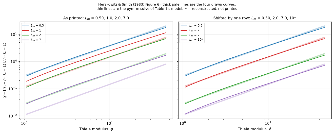
Deviations, both readings
The comparison away from \(\phi = 10\) is model against the fitted straight line, since the CSV holds no raw points. Convention throughout: \((\text{model} - \text{figure})/\text{figure}\).
PHI_TAB = np.array([2, 3, 5, 7, 10, 15, 20, 30], float)


def deviations(closures=PAPER, solver=sph, L_rec=L_rec, slope=SLOPE):
    """Finite-volume chi against the fitted drawn lines, both readings, PHI_TAB and phi = 10."""
    out = {}
    out["shift"] = np.array([dev([solver.chi(p, L, closures=closures) for p in PHI_TAB],
                                 line_chi(PHI_TAB, i, slope)) for i, L in enumerate(L_SHIFT)])
    out["print"] = np.array([dev([solver.chi(p, L, closures=closures) for p in PHI_TAB],
                                 line_chi(PHI_TAB, i, slope)) for i, L in enumerate(L_LEGEND)])
    out["d10_shift"] = dev([solver.chi(10.0, L, closures=closures) for L in L_SHIFT], CHI10)
    # how much of curve 4's excess is the rounding of its reconstructed L_m to 10?
    out["c4_exact"] = dev([solver.chi(p, L_rec[3], closures=closures) for p in PHI_TAB],
                          line_chi(PHI_TAB, 3, slope))
    out["shift_worst"] = float(np.max(np.abs(out["shift"])))
    out["shift_worst_123"] = float(np.max(np.abs(out["shift"][:3])))
    out["print_worst"] = float(np.max(np.abs(out["print"])))
    out["c4_exact_worst"] = float(np.max(np.abs(out["c4_exact"])))
    return out


DEV = deviations()
dev_shift, dev_print, d10_shift = DEV["shift"], DEV["print"], DEV["d10_shift"]
SHIFT_WORST, SHIFT_WORST_123, PRINT_WORST = DEV["shift_worst"], DEV["shift_worst_123"], DEV["print_worst"]
C4_EXACT_WORST = DEV["c4_exact_worst"]

lines = ["Deviation (%) against the fitted drawn lines - SHIFTED reading",
         "  phi   " + "".join(f"  L_m={L:<7g}" for L in L_SHIFT)]
for j, p in enumerate(PHI_TAB):
    lines.append(f"  {p:<5.0f} " + "".join(f"{dev_shift[i, j]*100:+10.1f}" for i in range(4)))
lines += ["", "Deviation (%) against the fitted drawn lines - AS PRINTED",
          "  phi   " + "".join(f"  L_m={L:<7g}" for L in L_LEGEND)]
for j, p in enumerate(PHI_TAB):
    lines.append(f"  {p:<5.0f} " + "".join(f"{dev_print[i, j]*100:+10.1f}" for i in range(4)))
lines += ["", f"curve 4 with the reconstructed L_m = {L_rec[3]:.2f} instead of the rounded 10:",
          "  phi   " + "".join(f"{p:8.0f}" for p in PHI_TAB),
          "  dev   " + "".join(f"{v*100:+8.1f}" for v in DEV["c4_exact"]),
          f"  worst {C4_EXACT_WORST*100:.1f} % against {np.max(np.abs(dev_shift[3]))*100:.1f} % "
          "at L_m = 10 exactly, i.e. most of curve 4's",
          "  excess is the rounding, not a failure of the shifted reading."]
print("\n".join(lines))
Deviation (%) against the fitted drawn lines - SHIFTED reading
phi L_m=0.5 L_m=2 L_m=7 L_m=10
2 +3.1 +2.7 +4.9 +13.3
3 +5.4 +5.3 +6.9 +14.6
5 +4.9 +5.2 +6.0 +12.5
7 +3.3 +3.9 +4.1 +9.9
10 +1.0 +1.9 +1.6 +6.4
15 -2.1 -1.0 -1.8 +2.1
20 -4.5 -3.2 -4.4 -1.1
30 -8.0 -6.4 -8.2 -5.7
Deviation (%) against the fitted drawn lines - AS PRINTED
phi L_m=0.5 L_m=1 L_m=2 L_m=7
2 +3.1 +70.7 +327.9 +168.1
3 +5.4 +75.0 +336.1 +171.1
5 +4.9 +74.8 +332.4 +166.2
7 +3.3 +72.7 +324.9 +159.9
10 +1.0 +69.2 +314.3 +151.8
15 -2.1 +64.5 +300.4 +141.5
20 -4.5 +60.9 +289.9 +133.9
30 -8.0 +55.5 +274.6 +123.0
curve 4 with the reconstructed L_m = 10.18 instead of the rounded 10:
phi 2 3 5 7 10 15 20 30
dev +6.5 +7.7 +5.7 +3.2 -0.0 -4.1 -7.1 -11.4
worst 11.4 % against 14.6 % at L_m = 10 exactly, i.e. most of curve 4's
excess is the rounding, not a failure of the shifted reading.display(Markdown(rf"""
At $\phi = 10$ the shifted reading gives
**{d10_shift[0]*100:+.1f} %, {d10_shift[1]*100:+.1f} %, {d10_shift[2]*100:+.1f} %**
and **{d10_shift[3]*100:+.1f} %**, against
{d_printed[0]*100:+.0f} %, {d_printed[1]*100:+.0f} %, {d_printed[2]*100:+.0f} %,
{d_printed[3]*100:+.0f} % as printed. Over $\phi$ = 2 to 30 the shifted reading
stays inside **{SHIFT_WORST_123*100:.0f} %** for the three curves that use only
printed $L_m$ values, and inside **{SHIFT_WORST*100:.0f} %** including the
reconstructed fourth at the round $L_m = 10$; as printed the worst is
**{PRINT_WORST*100:.0f} %**.
Curve 4 is the loose one for two reasons, and neither is the shifted reading.
About **{(1 - C4_EXACT_WORST/np.max(np.abs(dev_shift[3])))*100:.0f} %** of its
excess is the rounding of {L_rec[3]:.2f} to 10: at the
reconstructed value its worst deviation falls from
{np.max(np.abs(dev_shift[3]))*100:.1f} % to **{C4_EXACT_WORST*100:.1f} %**. The
rest is the slope residual of the next section: curve 4 is the steepest drawn
line ({SLOPE[3]:.3f}), so it is where the model's slope deficit shows most. The
page keeps the round 10 in the figure, because a fitted $L_m$ would make the
comparison circular, and reports both numbers.
"""))At \(\phi = 10\) the shifted reading gives +1.0 %, +1.9 %, +1.6 % and +6.4 %, against +1 %, +69 %, +314 %, +152 % as printed. Over \(\phi\) = 2 to 30 the shifted reading stays inside 8 % for the three curves that use only printed \(L_m\) values, and inside 15 % including the reconstructed fourth at the round \(L_m = 10\); as printed the worst is 336 %.
Curve 4 is the loose one for two reasons, and neither is the shifted reading. About 22 % of its excess is the rounding of 10.18 to 10: at the reconstructed value its worst deviation falls from 14.6 % to 11.4 %. The rest is the slope residual of the next section: curve 4 is the steepest drawn line (1.131), so it is where the model’s slope deficit shows most. The page keeps the round 10 in the figure, because a fitted \(L_m\) would make the comparison circular, and reports both numbers.
DIG = float(CHI_ERR_PCT.mean())          # the fits' own rms, expressed as % in chi

fig, axes = plt.subplots(1, 2, figsize=(12.4, 4.4), sharey=True)
for ax, (d, labels, title) in zip(axes, [
        (dev_print, L_LEGEND, "As printed"),
        (dev_shift, L_SHIFT, "Shifted by one row")]):
    for i, L in enumerate(labels):
        ax.semilogx(PHI_TAB, d[i] * 100, "o-", color=COL[i], ms=4, lw=1.3,
                    label=rf"$L_m$ = {L:g}" + ("*" if L == 10.0 else ""))
    ax.axhline(0, color="k", lw=1.0)
    ax.axhspan(-DIG, DIG, color="tab:green", alpha=0.10)
    ax.set_xlabel(r"$\phi$")
    ax.set_title(title, fontsize=10)
    ax.legend(fontsize=8)
axes[0].set_ylabel("deviation  (model - figure)/figure  [%]")
axes[0].set_yscale("symlog", linthresh=20)
axes[1].text(2.2, DIG + 2.0, f"digitisation rms, ~{DIG:.1f} % in chi",
             fontsize=8, color="tab:green")
fig.tight_layout()
plt.show()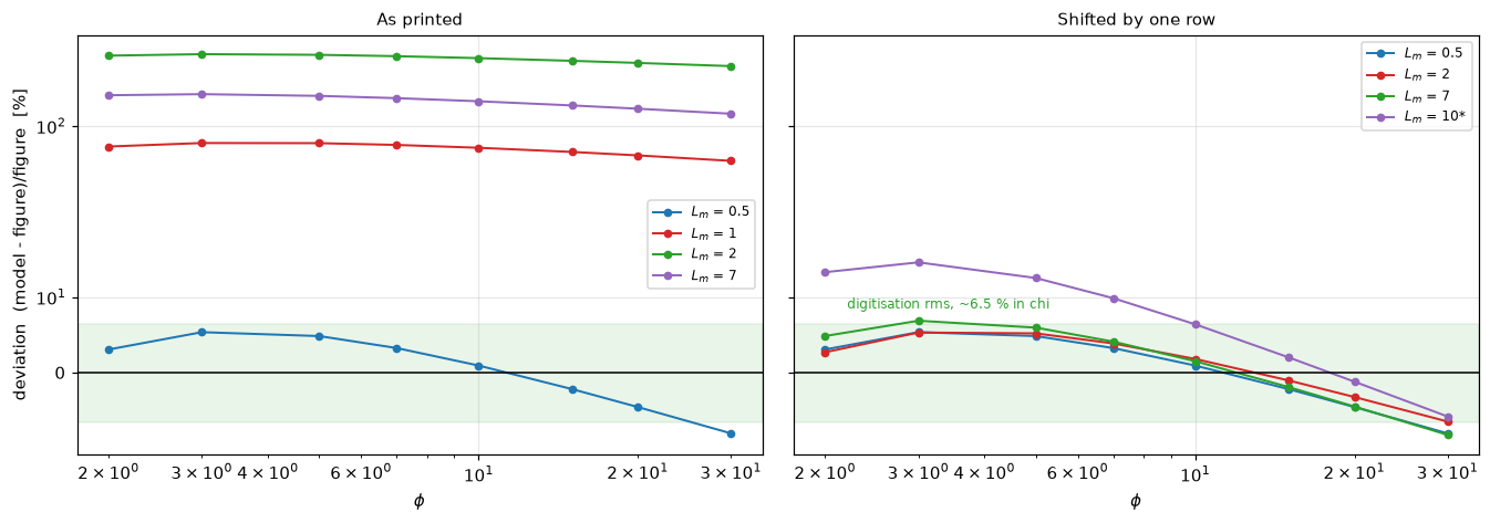
What the shift does not fix
The deviations under the shifted reading are not flat. They run positive at low \(\phi\) and negative at high \(\phi\), with the same shape on all four curves. That is a slope difference, and it survives the reassignment.
The dominant uncertainty on that difference is not the fit rms but the abscissa calibration. A log–log slope is (decades in \(\chi\))/(decades in \(\phi\)), so it scales linearly with the px per decade assumed on the \(\phi\) axis. The four labelled verticals (\(\phi\) = 1, 5, 10, 50) do not sit on a common logarithmic ruler (the \(\phi = 10\) gridline is off the line the other three define, as the sidecar records), so the CSV’s calibration is not the only defensible one. slope_stats rescales this CSV’s slopes to each recorded reading of the verticals.
DEC = np.log10(PHI_HI / PHI_LO)


def e2e(gap, dec=DEC):
    """A slope gap, accumulated over the digitised window, as a percentage in chi."""
    return (10.0 ** (gap * dec) - 1.0) * 100.0


def slope_stats(length_ratio=3.0, slope=SLOPE, phi_lo=PHI_LO, phi_hi=PHI_HI):
    """The model's straight-line fit over the window, and its gap to the drawn lines."""
    phis = np.logspace(np.log10(phi_lo), np.log10(phi_hi), 60)
    A = np.vstack([np.log10(phis), np.ones_like(phis)]).T
    lc = np.log10(chi_collapsed(phis, 2.0, length_ratio=length_ratio))
    (m_slope, m_int), *_ = np.linalg.lstsq(A, lc, rcond=None)
    out = {"model_slope": float(m_slope),
           "fit_rms": float(np.sqrt(np.mean((A @ [m_slope, m_int] - lc) ** 2))),
           # chi_collapsed(phi, L) = (1-f_e(L)) [eta_s(phi) phi^2] / a_gLs(L): the
           # phi-dependence is one factor, so the log-log SLOPE is the same for every L_m
           "slopes_all_L": [float(np.linalg.lstsq(A, np.log10(chi_collapsed(
               phis, L, length_ratio=length_ratio)), rcond=None)[0][0]) for L in L_SHIFT],
           "fig_mean": float(slope.mean()), "fig_min": float(slope.min()),
           "fig_max": float(slope.max())}
    out["gap"] = out["fig_mean"] - out["model_slope"]
    out["by_cal"] = {lab: out["fig_mean"] * cal / CAL_CSV - out["model_slope"]
                     for lab, cal in [("as digitised (this CSV)", CAL_CSV)] + list(CAL_ALT.items())}
    # the re-trace's refit gap is a derived number the sidecar records (it is the
    # re-fitted figure slope minus the model slope; the refit slope itself was not kept)
    out["gap_lo"] = float(min(min(out["by_cal"].values()), INDEP["derived_smallest_gap_on_refit"]))
    out["gap_hi"] = float(max(out["by_cal"].values()))
    out["dec"] = float(np.log10(phi_hi / phi_lo))
    return out


def local_slope(phi):
    d = 1e-6
    return float((np.log(chi_collapsed(phi * (1 + d), 2.0)) - np.log(chi_collapsed(phi * (1 - d), 2.0)))
                 / (np.log1p(d) - np.log1p(-d)))


SL = slope_stats()
model_slope, model_fit_rms = SL["model_slope"], SL["fit_rms"]
SLOPE_GAP, SLOPE_GAP_LO, SLOPE_GAP_HI = SL["gap"], SL["gap_lo"], SL["gap_hi"]
INDEP_GAP = INDEP["mean_slope"] - model_slope


def retrace_gap(slope=SLOPE):
    """|this CSV's mean slope rescaled to the re-trace's calibration - the re-trace's|."""
    return abs(slope.mean() * INDEP["px_per_decade"] / CAL_CSV - INDEP["mean_slope"])


RETRACE_GAP = retrace_gap()

lines = ["The model is not a straight line on these axes.",
         "  phi        1.07     2       5      10      20     45.5",
         "  local slope " + "".join(f"{local_slope(p):7.3f}" for p in (1.07, 2, 5, 10, 20, 45.5)),
         "",
         f"  best straight-line fit of the model over phi = {PHI_LO}-{PHI_HI}:",
         f"    slope {model_slope:.4f}   rms {model_fit_rms:.4f} decades",
         f"    (identical for all four L_m: {['%.4f' % s for s in SL['slopes_all_L']]})",
         "  the four digitised lines:",
         f"    slopes {['%.4f' % s for s in SLOPE]}   mean {SLOPE.mean():.4f}",
         f"    fit rms {['%.4f' % r for r in RMS_FIT]} decades",
         "",
         "Sensitivity of the slope gap to the abscissa calibration",
         "  px/decade  reading of the phi verticals    mean slope   gap      end-to-end"]
for lab, cal in [("as digitised (this CSV)", CAL_CSV)] + list(CAL_ALT.items()):
    g = SL["by_cal"][lab]
    lines.append(f"  {cal:8.1f}  {lab:<30} {g + model_slope:8.4f}  {g:+7.3f}  {e2e(g):+8.0f} %")
lines += ["",
          f"  independent re-trace, measured directly at {INDEP['px_per_decade']} px/decade: "
          f"mean slope {INDEP['mean_slope']:.4f}",
          f"  the same calibration applied to THIS CSV by rescaling:      "
          f"{SLOPE.mean()*INDEP['px_per_decade']/CAL_CSV:.4f}",
          "  -> the two digitisations differ by calibration alone, not by tracing.",
          f"  smallest gap the re-trace obtained by re-fitting (sidecar, derived): "
          f"{INDEP['derived_smallest_gap_on_refit']:+.3f}",
          "",
          f"  defensible range for the gap: {SLOPE_GAP_LO:+.3f} to {SLOPE_GAP_HI:+.3f}"
          f"  ({e2e(SLOPE_GAP_LO):+.0f} % to {e2e(SLOPE_GAP_HI):+.0f} % end to end)",
          "  The SIGN survives every one of them. The SIZE does not."]
print("\n".join(lines))
The model is not a straight line on these axes.
phi 1.07 2 5 10 20 45.5
local slope 1.420 1.200 1.071 1.034 1.017 1.007
best straight-line fit of the model over phi = 1.07-45.5:
slope 1.0767 rms 0.0189 decades
(identical for all four L_m: ['1.0767', '1.0767', '1.0767', '1.0767'])
the four digitised lines:
slopes ['1.1051', '1.0976', '1.1122', '1.1311'] mean 1.1115
fit rms ['0.0290', '0.0282', '0.0289', '0.0235'] decades
Sensitivity of the slope gap to the abscissa calibration
px/decade reading of the phi verticals mean slope gap end-to-end
421.9 as digitised (this CSV) 1.1115 +0.035 +14 %
418.6 4-point least squares 1.1028 +0.026 +10 %
417.8 3-point, phi = 10 dropped 1.1007 +0.024 +9 %
426.0 phi = 1 -> 10 baseline only 1.1223 +0.046 +19 %
independent re-trace, measured directly at 418.6 px/decade: mean slope 1.1028
the same calibration applied to THIS CSV by rescaling: 1.1028
-> the two digitisations differ by calibration alone, not by tracing.
smallest gap the re-trace obtained by re-fitting (sidecar, derived): +0.007
defensible range for the gap: +0.007 to +0.046 (+3 % to +19 % end to end)
The SIGN survives every one of them. The SIZE does not.end_to_end = e2e(SLOPE_GAP)
display(Markdown(rf"""
**The residual tilt, stated honestly.** The model's log–log slope is not a
single number: it falls from {local_slope(1.07):.2f} at
$\phi = {PHI_LO}$ to {local_slope(45.5):.2f} at $\phi = {PHI_HI}$, because
$\eta_s\phi^2 \to \phi$ only asymptotically. Its best straight-line fit over
the digitised window has slope **{model_slope:.3f}**. The four drawn curves,
reduced to straight lines by the same kind of fit, measure
**{SLOPE[0]:.3f}, {SLOPE[1]:.3f}, {SLOPE[2]:.3f}, {SLOPE[3]:.3f}**, mean
{SLOPE.mean():.3f}. The drawn lines are the steeper ones.
**The sign of the gap is solid; its size is not.** As digitised it is
{SLOPE_GAP:+.3f} in slope, {end_to_end:+.0f} % end to end over the
{DEC:.2f} decades of the window. But the dominant uncertainty is the
**abscissa calibration**, the weak axis of this figure. An
independent re-digitisation of the same figure, calibrating the abscissa
at {INDEP['px_per_decade']} px/decade, measures a mean slope of
**{INDEP['mean_slope']:.4f}**, a gap of **{INDEP_GAP:+.3f}**
({e2e(INDEP_GAP):+.0f} % end to end), and that is this CSV's
{SLOPE.mean():.4f} rescaled by the ratio of the two calibrations
({SLOPE.mean()*INDEP['px_per_decade']/CAL_CSV:.4f}). The two traces agree; only
their rulers differ. Across the defensible calibrations the gap runs from
**{SLOPE_GAP_LO:+.3f}** to **{SLOPE_GAP_HI:+.3f}**
({e2e(SLOPE_GAP_LO):+.0f} % to {e2e(SLOPE_GAP_HI):+.0f} % end to end). **The page
quotes the range, not a single number.**
**What does not defend it.** All four measured slopes lie above
{model_slope:.3f}, but that is *not* a scatter argument and this page does not
use it as one: all four were traced against **one** abscissa calibration, so a
common-mode error in that calibration moves all four together. Four numbers that
look like four samples are one measurement.
**It is unexplained, and it is not the legend misalignment.** The collapsed chain
factorises as $(1-f_e)\,\alpha_{{gLs}}^{{-1}}$ times $\eta_s(\phi)\phi^2$, so
$L_m$ moves a curve up and down and **cannot change its slope at all**: every
$L_m$ gives the identical {model_slope:.3f}. Reassigning curves therefore has
exactly zero effect on this residual, and it would be there under any reading.
A second, smaller caveat, quantified rather than assumed away: the model's own
best straight line leaves an rms of **{model_fit_rms:.3f} decades**, comparable
to the digitisation's {RMS_FIT.min():.3f}–{RMS_FIT.max():.3f}. So the reduction
of each drawn curve to a straight line discards curvature of the same size as the
model's, and the CSV cannot distinguish a straight line from this model's curve.
The discrepancy is reported as open, with its size as a range.
"""))The residual tilt, stated honestly. The model’s log–log slope is not a single number: it falls from 1.42 at \(\phi = 1.07\) to 1.01 at \(\phi = 45.5\), because \(\eta_s\phi^2 \to \phi\) only asymptotically. Its best straight-line fit over the digitised window has slope 1.077. The four drawn curves, reduced to straight lines by the same kind of fit, measure 1.105, 1.098, 1.112, 1.131, mean 1.111. The drawn lines are the steeper ones.
The sign of the gap is solid; its size is not. As digitised it is +0.035 in slope, +14 % end to end over the 1.63 decades of the window. But the dominant uncertainty is the abscissa calibration, the weak axis of this figure. An independent re-digitisation of the same figure, calibrating the abscissa at 418.6 px/decade, measures a mean slope of 1.1028, a gap of +0.026 (+10 % end to end), and that is this CSV’s 1.1115 rescaled by the ratio of the two calibrations (1.1028). The two traces agree; only their rulers differ. Across the defensible calibrations the gap runs from +0.007 to +0.046 (+3 % to +19 % end to end). The page quotes the range, not a single number.
What does not defend it. All four measured slopes lie above 1.077, but that is not a scatter argument and this page does not use it as one: all four were traced against one abscissa calibration, so a common-mode error in that calibration moves all four together. Four numbers that look like four samples are one measurement.
It is unexplained, and it is not the legend misalignment. The collapsed chain factorises as \((1-f_e)\,\alpha_{gLs}^{-1}\) times \(\eta_s(\phi)\phi^2\), so \(L_m\) moves a curve up and down and cannot change its slope at all: every \(L_m\) gives the identical 1.077. Reassigning curves therefore has exactly zero effect on this residual, and it would be there under any reading.
A second, smaller caveat, quantified rather than assumed away: the model’s own best straight line leaves an rms of 0.019 decades, comparable to the digitisation’s 0.024–0.029. So the reduction of each drawn curve to a straight line discards curvature of the same size as the model’s, and the CSV cannot distinguish a straight line from this model’s curve. The discrepancy is reported as open, with its size as a range.
Validation
Ranked before any code was written, highest available first. Every check below is followed by a deliberate break: a defect it is supposed to catch is injected and the number is measured again. A check whose number does not move is decoration, and this page names the ones that do not.
| # | check | what it is | can it fail? |
|---|---|---|---|
| 1 | Eq. 20 vs the \(f_e\) printed inside the figure | printed intermediate | yes |
| 2 | pymrm finite volume vs Table 1’s sphere row | independent routes | yes |
| 3 | grid convergence of the pymrm solve | discretisation | yes |
| 4 | the shift reconstruction | reconstruction vs printed values | yes |
| 5 | the collapse vs the full Table 1 chain | algebraic identity | no |
| 6 | \(\alpha_{gs}\to\infty\) sensitivity | assumption audit | n/a, a sweep |
1, 2 and 4, and what breaks them
def check_eq20(closures=PAPER):
    """max |Eq. 20 - printed f_e| over the four legend rows."""
    return float(np.max(np.abs(closures.f_e(L_LEGEND) - FE_PRINTED)))


def check_pymrm_vs_table1(n_u=800, nu=2, n_scale=3.0, L=2.0, phis=None):
    """max relative deviation of the finite-volume eta from Table 1's sphere row."""
    s = WettedSphere(n_u=n_u, nu=nu, n_scale=n_scale)
    a = float(PAPER.alpha_gLs(L))
    ps = PHI if phis is None else np.asarray(phis, float)
    num = np.array([s.eta(s.solve(p, a)) for p in ps])
    ana = 1.0 / (ps ** 2 / a + 1.0 / eta_sphere(ps))
    return float(np.max(np.abs(num / ana - 1.0)))


def check_reconstruction(closures=PAPER, chi_scale=1.0):
    """The three reconstructed L_m that the shift hypothesis predicts to be 0.5/2/7.

    Returns the max relative distance from those printed values. `chi_scale`
    corrupts the ORDINATE calibration instead of the algebra.
    """
    return float(max(abs(reconstruct_L(c, 10.0, closures) / t - 1.0)
                     for c, t in zip(CHI10[:3] * chi_scale, [0.5, 2.0, 7.0])))


BASE = {"eq20": check_eq20(), "pymrm": check_pymrm_vs_table1(), "recon": check_reconstruction()}
print("baselines:", {k: f"{v:.3e}" for k, v in BASE.items()})
baselines: {'eq20': '4.734e-03', 'pymrm': '7.727e-06', 'recon': '2.298e-02'}EQ20_DEFECTS = [("Eq. 20 exponent 0.1 -> 0.01", Closures(fe_expo=0.01), "mis-read superscript"),
("Eq. 20 exponent 0.1 -> 0.7", Closures(fe_expo=0.7), "mis-read superscript"),
("Eq. 20 coefficient 0.77 -> 0.87", Closures(fe_coef=0.87), "mis-read digit")]
EQ21_DEFECTS = [
("Eq. 21: 6.91 -> 6.31", Closures(c21=(1.05, 0.3, 6.31, 0.6)), "mis-read digit"),
("Eq. 21: 6.91 -> 6.71", Closures(c21=(1.05, 0.3, 6.71, 0.6)), "mis-read digit"),
("Eq. 21: 6.91 -> 7.91", Closures(c21=(1.05, 0.3, 7.91, 0.6)), "mis-read digit"),
("Eq. 21: 1.05 -> 1.95", Closures(c21=(1.95, 0.3, 6.91, 0.6)), "mis-read digit"),
("Eq. 21 exponent 0.6 -> 0.5", Closures(c21=(1.05, 0.3, 6.91, 0.5)), "mis-read superscript, 2nd term"),
("Eq. 21 exponent 0.6 -> 0.7", Closures(c21=(1.05, 0.3, 6.91, 0.7)), "mis-read superscript, 2nd term"),
("Eq. 21 exponents 0.3/0.6 -> 0.5/0.5", Closures(c21=(1.05, 0.5, 6.91, 0.5)), "mis-read superscripts")]
SOLVER_DEFECTS = [("nu = 0 (slab) not sphere", dict(nu=0), "wrong geometry"),
("nu = 1 (cylinder) not sphere", dict(nu=1), "wrong geometry"),
("Robin scale 3 -> 1 (n per R)", dict(n_scale=1.0), "length scale of dC/dn"),
("Robin scale 3 -> 9", dict(n_scale=9.0), "length scale of dC/dn"),
("n_u = 10", dict(n_u=10), "under-resolved grid"),
("n_u = 50", dict(n_u=50), "under-resolved grid")]
SCALE_DEFECTS = [("chi axis calibration x1.05", 1.05), ("chi axis calibration x0.95", 0.95)]
rows = [("(baseline)", BASE["eq20"], BASE["pymrm"], BASE["recon"], "")]
for lab, cl, note in EQ20_DEFECTS:
rows.append((lab, check_eq20(cl), None, check_reconstruction(cl), note))
for lab, kw, note in SOLVER_DEFECTS:
rows.append((lab, None, check_pymrm_vs_table1(**kw), None, note))
for lab, cl, note in EQ21_DEFECTS:
rows.append((lab, None, None, check_reconstruction(cl),
note + (" - IMPROVES the metric" if lab.endswith("7.91") else "")))
for lab, f in SCALE_DEFECTS:
rows.append((lab, None, None, check_reconstruction(chi_scale=f),
"ordinate scale error, not a transcription defect"))
w = max(len(r[0]) for r in rows)
lines = [f"{'injected defect':<{w}} {'check 1':>10} {'check 2':>10} {'check 4':>10} note",
"-" * (w + 50)]
for lab, a, b, c, n in rows:
cells = [f"{v:10.3e}" if v is not None else " " * 10 for v in (a, b, c)]
lines.append(f"{lab:<{w}} {cells[0]} {cells[1]} {cells[2]} {n}")
print("\n".join(lines))injected defect check 1 check 2 check 4 note
-------------------------------------------------------------------------------------
(baseline) 4.734e-03 7.727e-06 2.298e-02
Eq. 20 exponent 0.1 -> 0.01 1.549e-01 2.992e+01 mis-read superscript
Eq. 20 exponent 0.1 -> 0.7 2.066e+00 8.034e-01 mis-read superscript
Eq. 20 coefficient 0.77 -> 0.87 1.169e-01 6.393e-01 mis-read digit
nu = 0 (slab) not sphere 6.666e-01 wrong geometry
nu = 1 (cylinder) not sphere 3.333e-01 wrong geometry
Robin scale 3 -> 1 (n per R) 1.999e+00 length scale of dC/dn
Robin scale 3 -> 9 6.667e-01 length scale of dC/dn
n_u = 10 9.390e-02 under-resolved grid
n_u = 50 9.482e-03 under-resolved grid
Eq. 21: 6.91 -> 6.31 4.140e-02 mis-read digit
Eq. 21: 6.91 -> 6.71 2.708e-02 mis-read digit
Eq. 21: 6.91 -> 7.91 1.719e-02 mis-read digit - IMPROVES the metric
Eq. 21: 1.05 -> 1.95 5.475e-01 mis-read digit
Eq. 21 exponent 0.6 -> 0.5 3.332e-02 mis-read superscript, 2nd term
Eq. 21 exponent 0.6 -> 0.7 3.432e-02 mis-read superscript, 2nd term
Eq. 21 exponents 0.3/0.6 -> 0.5/0.5 1.680e-01 mis-read superscripts
chi axis calibration x1.05 6.295e-02 ordinate scale error, not a transcription defect
chi axis calibration x0.95 1.059e-01 ordinate scale error, not a transcription defect# --- check 4's real limits, measured rather than asserted --------------------
def check4_limits(chi_scale=1.0):
"""The transcription defects check 4 would not reject, with the curve positions
read at ordinate scale `chi_scale`. Returns the tolerance, the defect values,
the best unrejected defect and the baseline."""
tol = positions(chi10=CHI10 * chi_scale)["L_tol_pct"][:3]
vals = {lab: check_reconstruction(cl, chi_scale) for lab, cl, _ in EQ20_DEFECTS + EQ21_DEFECTS}
unrej = sorted((v, lab) for lab, v in vals.items() if v * 100 < tol.min())
return {"tol_min": float(tol.min()), "tol_max": float(tol.max()), "values": vals,
"unrejected": unrej, "best": unrej[0][0], "best_label": unrej[0][1],
"base": check_reconstruction(chi_scale=chi_scale)}
C4 = check4_limits()
L_TOL_MIN = C4["tol_min"]
CHECK4_BEST_DEFECT = C4["best"]
# WHY: at L_m ~ 1 the first term of Eq. 21 carries almost all of 1/alpha_gLs
def share_first(closures=PAPER, L=1.0):
c = closures.c21
inv1, inv2 = 1.0 / (c[0] * L ** c[1]), 1.0 / (c[2] * L ** c[3])
return inv1 / (inv1 + inv2)
SHARE_FIRST = share_first()
S_UP = check_reconstruction(chi_scale=1.05)
S_DN = check_reconstruction(chi_scale=0.95)
moved = {
"check 1 (Eq. 20 vs printed $f_e$)": ([r[1] for r in rows[1:] if r[1] is not None], BASE["eq20"]),
"check 2 (pymrm vs Table 1)": ([r[2] for r in rows[1:] if r[2] is not None], BASE["pymrm"]),
"check 4 (the reconstruction)": ([r[3] for r in rows[1:] if r[3] is not None], BASE["recon"]),
}
md = []
for k, (vals, b) in moved.items():
ratios = sorted(v / b for v in vals)
if ratios[0] < 1.0:
md.append(f"- **{k}**: baseline {b:.2e}; the injected defects move it by factors "
f"{ratios[0]:.2f}x to {ratios[-1]:.0f}x, and the smallest is **below 1**, "
f"i.e. one defect makes the metric look *better* than the undamaged chain.")
else:
md.append(f"- **{k}**: baseline {b:.2e}; every injected defect moved it, "
f"by factors {ratios[0]:.0f}x to {ratios[-1]:.0f}x.")
md.append(
f"- **but check 4 is only as sharp as the digitisation.** Its tolerance is "
f"{L_TOL_MIN:.1f}–{C4['tol_max']:.1f} % in $L_m$, set by the fits' own rms, against a "
f"baseline of {BASE['recon']*100:.2f} %. **{len(C4['unrejected'])}** of the injected "
f"transcription defects stay under even the tightest of those bars and so would **not** "
f"be rejected: " + ", ".join(f"`{lab}` ({v*100:.2f} %)" for v, lab in C4["unrejected"])
+ f". The first of them, `{C4['best_label']}`, comes in at **{CHECK4_BEST_DEFECT*100:.2f} %**, "
f"*better* than the undamaged {BASE['recon']*100:.2f} %, so a larger number here is not "
f"even monotone in the size of the defect.")
md.append(
f"- **The reason is structural, not statistical.** At $L_m \\approx 1$ the "
f"$1.05\\,L_m^{{0.3}}$ term carries **{SHARE_FIRST*100:.0f} %** of "
f"$1/\\alpha_{{gLs}}$, leaving the $6.91\\,L_m^{{0.6}}$ term only "
f"{(1-SHARE_FIRST)*100:.0f} %, so corrupting the second term barely moves $\\chi$ at all. "
f"Check 4 catches errors in Eq. 20 and in Eq. 21's **first** term; against Eq. 21's "
f"**second** term it is essentially blind, and the page claims nothing more for it.")
md.append(
f"- **It is also weak against an ordinate-scale error.** Rescaling the whole $\\chi$ "
f"calibration by ±5 % leaves it at {S_UP*100:.1f} % / {S_DN*100:.1f} %, inside the band, "
f"so unrejected. That is precisely the error class the curve-spacing test above *does* "
f"cover, and it is the honest reason to keep that test even though it is not an "
f"independent witness.")
display(Markdown("Every injected defect moves the check it is aimed at, but moving is not "
"rejecting:\n\n" + "\n".join(md)))Every injected defect moves the check it is aimed at, but moving is not rejecting:
- check 1 (Eq. 20 vs printed \(f_e\)): baseline 4.73e-03; every injected defect moved it, by factors 25x to 436x.
- check 2 (pymrm vs Table 1): baseline 7.73e-06; every injected defect moved it, by factors 1227x to 258696x.
- check 4 (the reconstruction): baseline 2.30e-02; the injected defects move it by factors 0.75x to 1302x, and the smallest is below 1, i.e. one defect makes the metric look better than the undamaged chain.
- but check 4 is only as sharp as the digitisation. Its tolerance is 3.8–11.4 % in \(L_m\), set by the fits’ own rms, against a baseline of 2.30 %. 4 of the injected transcription defects stay under even the tightest of those bars and so would not be rejected:
Eq. 21: 6.91 -> 7.91(1.72 %),Eq. 21: 6.91 -> 6.71(2.71 %),Eq. 21 exponent 0.6 -> 0.5(3.33 %),Eq. 21 exponent 0.6 -> 0.7(3.43 %). The first of them,Eq. 21: 6.91 -> 7.91, comes in at 1.72 %, better than the undamaged 2.30 %, so a larger number here is not even monotone in the size of the defect. - The reason is structural, not statistical. At \(L_m \approx 1\) the \(1.05\,L_m^{0.3}\) term carries 87 % of \(1/\alpha_{gLs}\), leaving the \(6.91\,L_m^{0.6}\) term only 13 %, so corrupting the second term barely moves \(\chi\) at all. Check 4 catches errors in Eq. 20 and in Eq. 21’s first term; against Eq. 21’s second term it is essentially blind, and the page claims nothing more for it.
- It is also weak against an ordinate-scale error. Rescaling the whole \(\chi\) calibration by ±5 % leaves it at 6.3 % / 10.6 %, inside the band, so unrejected. That is precisely the error class the curve-spacing test above does cover, and it is the honest reason to keep that test even though it is not an independent witness.
3. Grid convergence
The pymrm/Table 1 comparison is only a transcription check if the discretisation error is smaller than what it is meant to detect. Refine and measure the order, at three Thiele moduli: the surface layer is thinnest at the largest \(\phi\) in the window, and an order measured only there can be pre-asymptotic. Table 1 is the exact solution of the uniform Robin sphere at \(m = 1\), so the error is the discretisation error. Its round-off floor is measured by solving the finest grid twice, once through newton and once by a direct LU of the same linear system with a different column ordering; every error used for an order must lie at least 1e3 times above the declared bound on that gap. At the largest \(\phi\) one more grid, \(n_u\) = 6400, shows where the observed rate goes after its maximum.
GRIDS = (50, 100, 200, 400, 800, 1600, 3200)
PHI_GRID = (2.0, 10.0, PHI_HI)
NOISE_BOUND = 1e-11          # declared bound on the relative round-off of eta


def grid_errors(phi, grids=GRIDS, L=2.0, ref_factor=1.0):
    """|eta_FV / eta_Table1 - 1| on each grid (Robin, L_m = 2)."""
    a = float(PAPER.alpha_gLs(L))
    ana = ref_factor / (phi ** 2 / a + 1.0 / eta_sphere(phi))
    out = []
    for n in grids:
        s = WettedSphere(n_u=n)
        out.append(abs(s.eta(s.solve(phi, a)) / ana - 1.0))
    return np.array(out)


def orders(errs):
    """Observed orders between successive grids, read as doublings."""
    return np.log2(errs[:-1] / errs[1:])


def two_solver_gap(phi, n_u=GRIDS[-1], L=2.0):
    """|eta(newton) / eta(direct LU, natural ordering) - 1| on one grid."""
    s = WettedSphere(n_u=n_u)
    a = float(PAPER.alpha_gLs(L))
    lap, lap_bc = s.operators(a, 1.0)
    A = (lap - (3.0 * phi) ** 2 * eye_array(n_u, format="csc")).tocsc()
    y_lu = splu(A, permc_spec="NATURAL").solve(-lap_bc.ravel())
    return abs(s.eta(s.solve(phi, a)) / s.eta(y_lu) - 1.0)


GRIDS_HI = GRIDS + (6400,)   # phi_max only: past the maximum of the observed rate
GRIDS_OF = {2.0: GRIDS, 10.0: GRIDS, PHI_HI: GRIDS_HI}
ERRS = {p: grid_errors(p, GRIDS_OF[p]) for p in PHI_GRID}
ORD = {p: orders(e) for p, e in ERRS.items()}
NOISE_GAP = max(two_solver_gap(p, GRIDS_OF[p][-1]) for p in PHI_GRID)
ERR_OVER_NOISE = min(e[-1] for e in ERRS.values()) / NOISE_BOUND
GRID_ORDER = float(max(ORD[PHI_HI]))          # the largest observed rate at phi_max
GRID_ORDER_AT = GRIDS_HI[int(np.argmax(ORD[PHI_HI]))]
GRID_ORDER_MIN = float(ORD[PHI_HI][0])

lines = ["|eta_FV / eta_Table1 - 1|, Robin, L_m = 2, and the observed order per doubling",
         "  n_u   " + "".join(f"   phi = {p:<5.4g}      " for p in PHI_GRID)]
for k, n in enumerate(GRIDS_HI):
    lines.append(f"  {n:<6}" + "".join(
        (f"  {ERRS[p][k]:.3e}  {'' if k == 0 else f'{ORD[p][k-1]:5.3f}':>5}    "
         if k < len(ERRS[p]) else " " * 23) for p in PHI_GRID).rstrip())
lines += ["",
          f"round-off floor: two-solver gap on each finest grid (here {NOISE_GAP:.1e}), "
          f"declared bound {NOISE_BOUND:.0e}",
          f"smallest finest-grid error over that bound: {ERR_OVER_NOISE:.2g}"]
print("\n".join(lines))
|eta_FV / eta_Table1 - 1|, Robin, L_m = 2, and the observed order per doubling
n_u phi = 2 phi = 10 phi = 45.5
50 1.440e-04 1.176e-03 9.482e-03
100 3.270e-05 2.138 1.842e-04 2.675 2.170e-03 2.128
200 7.750e-06 2.077 2.908e-05 2.663 3.745e-04 2.535
400 1.883e-06 2.041 4.938e-06 2.558 5.538e-05 2.758
800 4.640e-07 2.021 9.300e-07 2.409 7.727e-06 2.841
1600 1.152e-07 2.011 1.936e-07 2.264 1.078e-06 2.841
3200 2.868e-08 2.005 4.349e-08 2.154 1.573e-07 2.777
6400 2.494e-08 2.657
round-off floor: two-solver gap on each finest grid (here 6.4e-13), declared bound 1e-11
smallest finest-grid error over that bound: 2.5e+03display(Markdown(rf"""
**The scheme is second order; the larger rates at large $\phi$ are
pre-asymptotic.** At $\phi = 2$ the observed order settles at
**{ORD[2.0][-1]:.3f}** on the finest pair. At $\phi = 10$ it has come down to
**{ORD[10.0][-1]:.3f}** and is still falling. At $\phi = {PHI_HI}$, where the
surface layer is a few cells thick on the coarse grids, the observed rate rises
from {GRID_ORDER_MIN:.2f} to a plateau of about **{GRID_ORDER:.2f}** (largest
between $n_u$ = {GRID_ORDER_AT // 2} and {GRID_ORDER_AT}) and then falls:
{ORD[PHI_HI][-2]:.2f} and **{ORD[PHI_HI][-1]:.2f}** on the two finest pairs. That
is an error of the form $a h^2 + b h^3$ with a small $a$, in which the $h^3$ term
dominates until the grid is fine, not a third-order scheme. Every error used lies
at least {ERR_OVER_NOISE:.2g} times above the declared round-off bound, so none
of these rates is fitted to noise; the order the page publishes is 2, asymptotic
at $\phi = 2$, and the rates at $\phi = 10$ and {PHI_HI} are bounded between 2
and 3 as indicative.
For check 2 this means the comparison at $n_u = {sph.n_u}$ resolves Table 1 to
{ETA_MAXDEV:.1e}, far below anything a transcription defect produces (the
smallest break above moves it by a factor of
{min(r[2] for r in rows[1:] if r[2] is not None) / BASE['pymrm']:.0f}).
"""))The scheme is second order; the larger rates at large \(\phi\) are pre-asymptotic. At \(\phi = 2\) the observed order settles at 2.005 on the finest pair. At \(\phi = 10\) it has come down to 2.154 and is still falling. At \(\phi = 45.5\), where the surface layer is a few cells thick on the coarse grids, the observed rate rises from 2.13 to a plateau of about 2.84 (largest between \(n_u\) = 200 and 400) and then falls: 2.78 and 2.66 on the two finest pairs. That is an error of the form \(a h^2 + b h^3\) with a small \(a\), in which the \(h^3\) term dominates until the grid is fine, not a third-order scheme. Every error used lies at least 2.5e+03 times above the declared round-off bound, so none of these rates is fitted to noise; the order the page publishes is 2, asymptotic at \(\phi = 2\), and the rates at \(\phi = 10\) and 45.5 are bounded between 2 and 3 as indicative.
For check 2 this means the comparison at \(n_u = 800\) resolves Table 1 to 3.1e-04, far below anything a transcription defect produces (the smallest break above moves it by a factor of 1227).
5. The collapse: a check that cannot fail
chi_collapsed and chi_table1(..., alpha_gs=inf) agree to machine precision. They are the same algebra written twice: substituting \(\alpha_{gs}=\infty\) and \(C^*_L=1\) into Table 1’s row and cancelling gives the collapsed form line for line. It therefore cannot detect a mis-read coefficient in Table 1, a wrong length scale, or anything physical: a defect in the sphere row moves both sides identically. It is kept because it confirms the collapse step, which the page’s root finding relies on, and for no other reason.
The measurement below shows exactly that: a deliberately corrupted sphere row leaves the identity untouched while the pymrm comparison (check 2) blows up.
def identity_with_corrupt_sphere(fac):
    """check 5 (the collapse identity) evaluated with the sphere term multiplied by `fac`."""
    def eta_bad(phi):
        return eta_sphere(phi) / fac

    def full(phi, L):
        ie = 1.0 / eta_bad(phi)
        a, fe = float(PAPER.alpha_gLs(L)), float(PAPER.f_e(L))
        return (fe / (phi ** 2 / a + ie) + (1 - fe) * eta_bad(phi)) / (1.0 / (phi ** 2 / a + ie)) - 1

    def coll(phi, L):
        return (1 - float(PAPER.f_e(L))) * eta_bad(phi) * phi ** 2 / float(PAPER.alpha_gLs(L))

    p = np.logspace(0, 1.6, 20)
    return float(np.max(np.abs(coll(p, 2.0) / full(p, 2.0) - 1.0)))


def pymrm_vs_corrupt_sphere(fac, L=2.0):
    """check 2 evaluated against the SAME corrupted sphere term. Measured, not asserted."""
    a = float(PAPER.alpha_gLs(L))
    num = np.array([sph.eta(sph.solve(p, a)) for p in PHI])
    ana = 1.0 / (PHI ** 2 / a + fac / eta_sphere(PHI))
    return float(np.max(np.abs(num / ana - 1.0)))


lines = ["A corrupted sphere term, put through both checks",
         "  sphere term x   check 5 (identity)   check 2 (pymrm vs Table 1)"]
for fac in (1.0, 1.01, 1.5, 3.0):
    lines.append(f"  {fac:<15.2f} (here {identity_with_corrupt_sphere(fac):.1e})          "
                 f"{pymrm_vs_corrupt_sphere(fac):.2e}")
lines += ["", "  -> check 5 does not move at all; check 2 moves by the size of the defect.",
          "     The identity is blind to the very error it looks like it is testing."]
print("\n".join(lines))
A corrupted sphere term, put through both checks
sphere term x check 5 (identity) check 2 (pymrm vs Table 1)
1.00 (here 1.8e-15) 7.73e-06
1.01 (here 6.7e-16) 6.09e-03
1.50 (here 2.2e-15) 3.04e-01
3.00 (here 2.2e-15) 1.22e+00
-> check 5 does not move at all; check 2 moves by the size of the defect.
The identity is blind to the very error it looks like it is testing.6. Is an infinite gas-solid Biot number safe?
The paper says only “very large”. Every number on this page assumes literally infinite. That assumption is doing real work, and the sweep says how much.
def ags_cost(ags, phi=30.0, L=2.0, length_ratio=3.0):
    """chi at a finite alpha_gs relative to the alpha_gs -> inf limit, minus 1."""
    return float(chi_table1(phi, L, alpha_gs=ags, length_ratio=length_ratio)
                 / chi_collapsed(phi, L, length_ratio=length_ratio) - 1)


lines = ["chi under a FINITE gas-solid Biot number, relative to the infinite limit, L_m = 2",
         "  a_gs      phi=2      phi=10     phi=30"]
for ags in (10, 30, 100, 300, 1000, 3000):
    lines.append(f"  {ags:<9} " + "".join(f"{ags_cost(ags, p)*100:+9.2f}%" for p in (2.0, 10.0, 30.0)))
AGS_1000_AT30 = ags_cost(1000.0)
AGS_100_AT30 = ags_cost(100.0)
lines.append(f"\nfor scale, alpha_gLs itself is only {float(PAPER.alpha_gLs(0.5)):.2f} to "
             f"{float(PAPER.alpha_gLs(10.0)):.2f} over the four curves")
print("\n".join(lines))
chi under a FINITE gas-solid Biot number, relative to the infinite limit, L_m = 2
a_gs phi=2 phi=10 phi=30
10 -24.15% -55.00% -77.69%
30 -8.90% -27.27% -51.65%
100 -2.77% -9.86% -23.77%
300 -0.93% -3.49% -9.35%
1000 -0.28% -1.07% -2.99%
3000 -0.09% -0.36% -1.02%
for scale, alpha_gLs itself is only 0.72 to 1.95 over the four curvesdisplay(Markdown(rf"""
"Very large" has to mean *very*: at $\phi = 30$ even
$\alpha_{{gs}} = 1000$ still costs **{abs(AGS_1000_AT30)*100:.1f} %** in
$\chi$, and $\alpha_{{gs}} = 100$, already about
{100/float(PAPER.alpha_gLs(2.0)):.0f} times $\alpha_{{gLs}}$, costs
**{abs(AGS_100_AT30)*100:.0f} %**. The reconstruction above is
therefore **conditional on $\alpha_{{gs}} = \infty$ exactly**, and would return
different $L_m$ values under any finite value. The page states this as a
condition of its finding, not as a caveat buried in the code.
"""))“Very large” has to mean very: at \(\phi = 30\) even \(\alpha_{gs} = 1000\) still costs 3.0 % in \(\chi\), and \(\alpha_{gs} = 100\), already about 87 times \(\alpha_{gLs}\), costs 24 %. The reconstruction above is therefore conditional on \(\alpha_{gs} = \infty\) exactly, and would return different \(L_m\) values under any finite value. The page states this as a condition of its finding, not as a caveat buried in the code.
The alternative explanations, and why they lose
Before concluding the legend is misaligned, the two hypotheses that would rescue the printed reading are given their best chance. Each is fitted per curve, so each has four free parameters against four curves and must fit perfectly; the question is whether what it needs is physically admissible.
ALT A is a finite \(\alpha_{gs}\). alpha_gs_for finds it as a direct root: only the dry term of Table 1 depends on \(\alpha_{gs}\), and it increases with it, so \(\chi\) rises monotonically from \(f_e - 1\) at \(\alpha_{gs} = 0\) to the collapsed value at \(\alpha_{gs} \to \infty\). A root exists exactly when a curve sits below that limit; the bracket starts at \([1, 10]\) and each end is widened tenfold until it brackets. ALT B is a corrected \(f_e\); the collapsed \(\chi\) is linear in \(f_e\), so it is solved in closed form.
def alternatives(closures=PAPER):
    """ALT A (alpha_gs per curve) and ALT B (f_e per curve), printed reading kept."""
    alt_a = []
    for L, c in zip(L_LEGEND, CHI10):
        # a root exists only below the alpha_gs -> inf limit (no root is a result, not a failure)
        alt_a.append(alpha_gs_for(c, 10.0, L, closures)
                     if float(closures.f_e(L)) < 1.0 and c < float(chi_collapsed(10.0, L, closures))
                     else np.nan)
    alt_a = np.array(alt_a)
    # chi = (1 - f_e) eta_s(10) 10^2 / a_gLs is linear in f_e
    alt_b = 1.0 - CHI10 * closures.alpha_gLs(L_LEGEND) / (float(eta_sphere(10.0)) * 100.0)
    lb, lf = np.log(L_LEGEND), np.log(alt_b)
    slopes = np.diff(lf) / np.diff(lb)
    n_pl = float((lf[-1] - lf[0]) / (lb[-1] - lb[0]))   # pinned to the two extreme values,
    c_pl = float(alt_b[0] / L_LEGEND[0] ** n_pl)        # the kindest single power law
    pl = c_pl * L_LEGEND ** n_pl
    miss = pl / alt_b - 1.0
    return {"alt_a": alt_a, "alt_b": alt_b, "slopes": slopes, "n_pl": n_pl, "c_pl": c_pl,
            "pl": pl, "miss": miss, "pl_worst": float(np.max(np.abs(miss))),
            "a_spread": float(np.nanmax(alt_a) / np.nanmin(alt_a))}


ALT = alternatives()
alt_a, alt_b = ALT["alt_a"], ALT["alt_b"]
ALTB_SLOPES, ALTB_PL_MISS, ALTB_PL_WORST = ALT["slopes"], ALT["miss"], ALT["pl_worst"]
C_PL, N_PL = ALT["c_pl"], ALT["n_pl"]

lines = ["ALT A - a finite alpha_gs rescuing the printed reading (fitted per curve at phi = 10)"]
for L, r in zip(L_LEGEND, alt_a):
    lines.append(f"  L_m = {L:<5} " + ("no admissible root" if np.isnan(r)
                                         else f"needs alpha_gs = {r:10.1f}"))
lines.append("\nALT B - a corrected f_e per curve (printed reading kept)")
for k, (L, r) in enumerate(zip(L_LEGEND, alt_b)):
    lines.append(f"  L_m = {L:<5} needs f_e = {r:.4f}   (Eq. 20 gives {float(PAPER.f_e(L)):.4f}, "
                 f"figure prints {FE_PRINTED[k]:.2f})")
lines += ["", "Is the required f_e(L_m) a power law at all?",
          "  L_m                     " + "".join(f"{L:9.2f}" for L in L_LEGEND),
          "  required f_e            " + "".join(f"{v:9.4f}" for v in alt_b),
          "  d log f_e / d log L_m       " + "".join(f"{v:9.3f}" for v in ALTB_SLOPES)
          + "   <- must be CONSTANT for a power law",
          f"  best power law {C_PL:.3f} L^{N_PL:.3f}" + "".join(f"{v:9.4f}" for v in ALT["pl"]),
          "  it misses by            " + "".join(f"{v*100:+8.1f}%" for v in ALTB_PL_MISS)]
print("\n".join(lines))
ALT A - a finite alpha_gs rescuing the printed reading (fitted per curve at phi = 10)
L_m = 0.5 needs alpha_gs = 1057.2
L_m = 1.0 needs alpha_gs = 16.2
L_m = 2.0 needs alpha_gs = 4.6
L_m = 7.0 needs alpha_gs = 9.2
ALT B - a corrected f_e per curve (printed reading kept)
L_m = 0.5 needs f_e = 0.7212 (Eq. 20 gives 0.7184, figure prints 0.72)
L_m = 1.0 needs f_e = 0.8641 (Eq. 20 gives 0.7700, figure prints 0.77)
L_m = 2.0 needs f_e = 0.9578 (Eq. 20 gives 0.8253, figure prints 0.83)
L_m = 7.0 needs f_e = 0.9743 (Eq. 20 gives 0.9354, figure prints 0.94)
Is the required f_e(L_m) a power law at all?
L_m 0.50 1.00 2.00 7.00
required f_e 0.7212 0.8641 0.9578 0.9743
d log f_e / d log L_m 0.261 0.149 0.014 <- must be CONSTANT for a power law
best power law 0.780 L^0.114 0.7212 0.7805 0.8447 0.9743
it misses by +0.0% -9.7% -11.8% +0.0%display(Markdown(rf"""
**ALT A fails on consistency.** One $\alpha_{{gs}}$ is stated for the whole
figure, but the four curves need
{alt_a[0]:.0f}, {alt_a[1]:.1f}, {alt_a[2]:.1f} and {alt_a[3]:.1f}, spread over
a factor of {ALT['a_spread']:.0f}, not monotone in $L_m$, and
three of the four far too small to be called "very large" when
$\alpha_{{gLs}}$ itself is only {float(PAPER.alpha_gLs(0.5)):.2f}–{float(PAPER.alpha_gLs(7.0)):.2f}.
**ALT B fails on two counts, and the first one is decisive on its own.** The
$f_e$ values it needs ({alt_b[0]:.4f}, {alt_b[1]:.4f}, {alt_b[2]:.4f},
{alt_b[3]:.4f}) **contradict the $f_e$ column printed inside the figure**
({FE_PRINTED[0]:.2f}, {FE_PRINTED[1]:.2f}, {FE_PRINTED[2]:.2f},
{FE_PRINTED[3]:.2f}), which Eq. 20 already reproduces to the printed precision.
The paper would have to disagree with its own legend.
It also fails on **curvature**. It is tempting to argue from the *correction* to
$f_e$ ({(alt_b[0]-float(PAPER.f_e(0.5)))*100:+.1f},
{(alt_b[1]-float(PAPER.f_e(1.0)))*100:+.1f}, {(alt_b[2]-float(PAPER.f_e(2.0)))*100:+.1f},
{(alt_b[3]-float(PAPER.f_e(7.0)))*100:+.1f} percentage points) being non-monotone, but
that proves nothing: a non-monotone *difference* between two monotone functions
is perfectly ordinary, and the required $f_e$ values themselves *are* monotone.
What actually excludes a power law is that a power law has a **constant** log–log
slope, and the required values do not: theirs run
**{ALTB_SLOPES[0]:.3f} → {ALTB_SLOPES[1]:.3f} → {ALTB_SLOPES[2]:.3f}**, strongly
concave. Pin the kindest single power law to the two extreme required values and
it is ${C_PL:.3f}\,L_m^{{{N_PL:.3f}}}$, which misses the middle two by
**{ALTB_PL_MISS[1]*100:+.1f} %** and **{ALTB_PL_MISS[2]*100:+.1f} %**. So no
rewriting of Eq. 20's coefficient or exponent reaches these values; it would take
a different correction per curve.
**The shift wins because it needs nothing.** It introduces no free parameter for
three of the four curves: it reuses 0.50, 2.0 and 7.0 exactly as printed, and
only the fourth curve needs a value the paper does not print. The curve positions
return those three to within {max(abs(POS['L_rec_reldiff_pct'][:3])):.1f} % in
$L_m$, and the curve spacings (*the same measurement with a common
multiplicative offset in $\chi$ removed, not a second witness*) come to
{gaps_fig[0]:.3f}/{gaps_fig[1]:.3f}/{gaps_fig[2]:.3f} against the shifted
reading's {g_shifted[0]:.3f}/{g_shifted[1]:.3f}/{g_shifted[2]:.3f}.
"""))ALT A fails on consistency. One \(\alpha_{gs}\) is stated for the whole figure, but the four curves need 1057, 16.2, 4.6 and 9.2, spread over a factor of 230, not monotone in \(L_m\), and three of the four far too small to be called “very large” when \(\alpha_{gLs}\) itself is only 0.72–1.74.
ALT B fails on two counts, and the first one is decisive on its own. The \(f_e\) values it needs (0.7212, 0.8641, 0.9578, 0.9743) contradict the \(f_e\) column printed inside the figure (0.72, 0.77, 0.83, 0.94), which Eq. 20 already reproduces to the printed precision. The paper would have to disagree with its own legend.
It also fails on curvature. It is tempting to argue from the correction to \(f_e\) (+0.3, +9.4, +13.3, +3.9 percentage points) being non-monotone, but that proves nothing: a non-monotone difference between two monotone functions is perfectly ordinary, and the required \(f_e\) values themselves are monotone. What actually excludes a power law is that a power law has a constant log–log slope, and the required values do not: theirs run 0.261 → 0.149 → 0.014, strongly concave. Pin the kindest single power law to the two extreme required values and it is \(0.780\,L_m^{0.114}\), which misses the middle two by -9.7 % and -11.8 %. So no rewriting of Eq. 20’s coefficient or exponent reaches these values; it would take a different correction per curve.
The shift wins because it needs nothing. It introduces no free parameter for three of the four curves: it reuses 0.50, 2.0 and 7.0 exactly as printed, and only the fourth curve needs a value the paper does not print. The curve positions return those three to within 2.3 % in \(L_m\), and the curve spacings (the same measurement with a common multiplicative offset in \(\chi\) removed, not a second witness) come to 0.415/0.609/0.394 against the shifted reading’s 0.412/0.611/0.374.
The general argument: chi separates
Both rivals above are fitted, and a fitted rival can always be answered with “then fit something else”. There is a stronger statement available, and it needs no fitting at all.
Every variant of Eqs. 20–21, and every unstated-parameter hypothesis that keeps the paper’s structure, makes \(\chi\) separable:
\[ \chi(\phi, L_m) = g(L_m)\,h(\phi), \qquad g = \frac{1 - f_e(L_m)}{\alpha_{gLs}(L_m)}, \qquad h = \eta_s(\phi)\,\phi^2 \]
All of the \(L_m\) dependence sits in \(g\). A gap between two curves, in decades, is then \(\log_{10} g(L_i)/g(L_j)\) whatever \(h\) is, so the figure’s three measured gaps, with nothing fitted and no model evaluated, force the value of \(d\log g/d\log L_m\) over whichever \(L_m\) intervals a reading assigns to them.
FORCED_PRINT, FORCED_SHIFT = POS["forced_print"], POS["forced_shift"]
MODEL_PRINT, MODEL_SHIFT = POS["model_print"], POS["model_shift"]
DLOGG_SHIFT_WORST = POS["dlogg_worst"]

lines = ["chi = g(L_m) h(phi), so the figure's gaps ALONE fix d log g / d log L_m"]
for name, Ls, f_, m_ in (("AS PRINTED", L_LEGEND, FORCED_PRINT, MODEL_PRINT),
                         ("SHIFTED   ", L_SHIFT, FORCED_SHIFT, MODEL_SHIFT)):
    ivs = "  ".join(f"[{Ls[i]:g},{Ls[i+1]:g}]".rjust(9) for i in range(3))
    lines += [f"\n  {name}  L_m = {', '.join('%g' % x for x in Ls)}",
              f"    interval                 {ivs}",
              "    forced by the figure  " + "".join(f"{v:11.3f}" for v in f_),
              "    the paper's own g     " + "".join(f"{v:11.3f}" for v in m_),
              "    relative difference   " + "".join(f"{(a/b-1)*100:+10.1f}%" for a, b in zip(f_, m_))]
lines += [f"\n  A power law in L_m would need this slope CONSTANT. Read as printed the figure",
          f"  demands {FORCED_PRINT[0]:.3f} -> {FORCED_PRINT[1]:.3f} -> {FORCED_PRINT[2]:.3f}:",
          "  not constant, and not even monotone - steeper in the middle than at either end."]
print("\n".join(lines))
chi = g(L_m) h(phi), so the figure's gaps ALONE fix d log g / d log L_m
AS PRINTED L_m = 0.5, 1, 2, 7
interval [0.5,1] [1,2] [2,7]
forced by the figure -1.380 -2.024 -0.725
the paper's own g -0.635 -0.733 -1.122
relative difference +117.3% +176.3% -35.4%
SHIFTED L_m = 0.5, 2, 7, 10
interval [0.5,2] [2,7] [7,10]
forced by the figure -0.690 -1.120 -2.546
the paper's own g -0.684 -1.122 -2.414
relative difference +0.9% -0.2% +5.4%
A power law in L_m would need this slope CONSTANT. Read as printed the figure
demands -1.380 -> -2.024 -> -0.725:
not constant, and not even monotone - steeper in the middle than at either end.display(Markdown(rf"""
Read **as printed**, the figure's own gaps demand
$d\log g/d\log L_m$ = **{FORCED_PRINT[0]:.3f}, {FORCED_PRINT[1]:.3f},
{FORCED_PRINT[2]:.3f}** over $[0.5, 1]$, $[1, 2]$ and $[2, 7]$. That is not
constant, so no product of powers of $L_m$ can supply it, which disposes of
every rewriting of Eq. 20 or Eq. 21 in one line. Worse, it is not even
**monotone**: it steepens to {FORCED_PRINT[1]:.3f} in the middle interval and
then flattens to {FORCED_PRINT[2]:.3f}. A power law would give a **constant**;
the paper's own closures give a **monotone steepening**
({MODEL_PRINT[0]:.3f} → {MODEL_PRINT[1]:.3f} → {MODEL_PRINT[2]:.3f} over these
same three intervals); the printed reading needs neither.
Read **shifted**, the *same three gaps* demand
**{FORCED_SHIFT[0]:.3f}, {FORCED_SHIFT[1]:.3f}, {FORCED_SHIFT[2]:.3f}** over
$[0.5, 2]$, $[2, 7]$ and $[7, 10]$, against the model's
**{MODEL_SHIFT[0]:.3f}, {MODEL_SHIFT[1]:.3f}, {MODEL_SHIFT[2]:.3f}**: agreement
to within **{DLOGG_SHIFT_WORST*100:.1f} %** on the worst interval, with nothing
fitted.
This is the strongest statement the page can make, because it does not depend on
which rival is proposed. Any hypothesis that leaves $\chi$ separable (a finite
$\alpha_{{gs}}$, a corrected $f_e$, different constants in Eq. 21, a different
correlation altogether) is fixed by these three numbers, and the printed reading
asks them for a shape no such $g$ has. **The printed reading is not recoverable
by any reparameterisation; only by a different assignment of $L_m$ to curves.**
(ALT A is the one escape from separability, since a finite $\alpha_{{gs}}$
couples $\phi$ and $L_m$, and it is refuted above on its own terms.)
"""))Read as printed, the figure’s own gaps demand \(d\log g/d\log L_m\) = -1.380, -2.024, -0.725 over \([0.5, 1]\), \([1, 2]\) and \([2, 7]\). That is not constant, so no product of powers of \(L_m\) can supply it, which disposes of every rewriting of Eq. 20 or Eq. 21 in one line. Worse, it is not even monotone: it steepens to -2.024 in the middle interval and then flattens to -0.725. A power law would give a constant; the paper’s own closures give a monotone steepening (-0.635 → -0.733 → -1.122 over these same three intervals); the printed reading needs neither.
Read shifted, the same three gaps demand -0.690, -1.120, -2.546 over \([0.5, 2]\), \([2, 7]\) and \([7, 10]\), against the model’s -0.684, -1.122, -2.414: agreement to within 5.4 % on the worst interval, with nothing fitted.
This is the strongest statement the page can make, because it does not depend on which rival is proposed. Any hypothesis that leaves \(\chi\) separable (a finite \(\alpha_{gs}\), a corrected \(f_e\), different constants in Eq. 21, a different correlation altogether) is fixed by these three numbers, and the printed reading asks them for a shape no such \(g\) has. The printed reading is not recoverable by any reparameterisation; only by a different assignment of \(L_m\) to curves. (ALT A is the one escape from separability, since a finite \(\alpha_{gs}\) couples \(\phi\) and \(L_m\), and it is refuted above on its own terms.)
What none of this can detect
Named as claims the page does not make:
- Eq. 6’s superposition is untested. Replacing a mixed-boundary sphere by a weighted average of two whole-surface spheres is the paper’s approximation (from Ramachandran & Smith 1979), and every route on this page (closed form, pymrm solve, reconstruction) is built on top of it. If it is wrong, all of them are wrong together. Testing it needs a 2-D axisymmetric solve of one sphere with two boundary patches, which is not attempted here.
- The constants inside Eq. 21 are untested. They came from the Goto & Smith and Specchia correlations evaluated at the caption’s conditions. Neither correlation is on disk; the page uses Eq. 21 as printed and cannot check the substitution.
- The mechanism of the misalignment is untested. See above: legend-vs-plot cannot be distinguished from the figure.
- Truncating the Newton iteration is not a defect check 2 can see at \(m = 1\), because the \(m = 1\) problem is linear and the first Newton step already lands on the solution, up to the finite-difference Jacobian that
NumJacbuilds (measured below). What keeps a non-converged solve out of every number is not check 2 butWettedSphere.solve, which raises whennewtondoes not report convergence. - No claim is made that the model is correct. It reproduces curves the authors computed from it. Figure 6 contains no measurements, and neither does this page.
def first_step_dev(m, n_u=200, phi=10.0, L=2.0):
    """|eta(first Newton iterate) / eta(converged) - 1| for an integer reaction order m.

    Plain Newton without bounds, so that the first step is the full Newton step
    (an integer order needs no bound at 0).
    """
    s = WettedSphere(n_u=n_u)
    a = float(PAPER.alpha_gLs(L))
    iterates = []
    r = newton(lambda y: s.residual(y, phi, a, 1.0, m), np.ones(s.shape), tol=s.tol,
               maxfev=60, callback=lambda x, g: iterates.append(x.copy()))
    if not r.success:
        raise RuntimeError(f"first_step_dev at m = {m:g}: {r.message}")
    return abs(s.eta(iterates[0], m) / s.eta(r.x, m) - 1.0)


M1_FIRST = first_step_dev(1)
print(f"m = 1 is linear: the first Newton step's eta is the converged one to (here {M1_FIRST:.1e})")
m = 1 is linear: the first Newton step's eta is the converged one to (here 2.6e-09)Summary
display(Markdown(rf"""
Reading Figure 6's legend as printed, the paper's own chain misses
three of its four curves by up to
{np.max(np.abs(d_printed))*100:.0f} %. Reading the legend as offset by one row
from its second entry down, so that the drawn curves are
$L_m$ = 0.50, 2.0, 7.0 and ≈10, brings all four to within
{np.max(np.abs(d10_shift))*100:.1f} % at $\phi = 10$ and
{SHIFT_WORST*100:.0f} % over $\phi$ = 2–30, with **nothing fitted** for the
three curves that reuse printed $L_m$ values.

Two further readings of the same figure support it, and neither is an
independent witness. The curve **spacings** (the same four positions with a
common multiplicative offset in $\chi$ removed) are matched by the shifted
reading to {GAP_MISS_SHIFT:.3f} decades, while the printed reading misses them by
up to {GAP_MISS_PRINT:.3f}. And because $\chi$ **separates** into $g(L_m)h(\phi)$,
those same three gaps force $d\log g/d\log L_m$ without any model at all: read
as printed they demand {FORCED_PRINT[0]:.3f}/{FORCED_PRINT[1]:.3f}/{FORCED_PRINT[2]:.3f},
which is non-monotone and so unreachable by any product of powers of $L_m$; read
shifted they demand {FORCED_SHIFT[0]:.3f}/{FORCED_SHIFT[1]:.3f}/{FORCED_SHIFT[2]:.3f}
against the model's {MODEL_SHIFT[0]:.3f}/{MODEL_SHIFT[1]:.3f}/{MODEL_SHIFT[2]:.3f}.
No reparameterisation rescues the printed reading; only a reassignment does.

One residual survives and is reported as unexplained: the drawn lines are
steeper than the model in log–log slope ({SLOPE.mean():.3f} against
{model_slope:.3f} as digitised). Its **sign** is robust, its **size** is not:
the abscissa calibration, not the fit rms, dominates, and across defensible
calibrations the gap spans {SLOPE_GAP_LO:+.3f} to {SLOPE_GAP_HI:+.3f}. $L_m$
cannot produce it either way, because the chain factorises.

The pymrm finite-volume solve reproduces Table 1's sphere row to
{ETA_MAXDEV:.1e} at $n_u$ = {sph.n_u}; the scheme is second order
({ORD[2.0][-1]:.2f} at $\phi = 2$), with a pre-asymptotic observed rate up to
{GRID_ORDER:.2f} at $\phi = {PHI_HI}$. Deviation is
(model − figure)/figure throughout. Tier 6: the "figure" is the authors' own
computed output, not a measurement.
"""))
Reading Figure 6’s legend as printed, the paper’s own chain misses three of its four curves by up to 314 %. Reading the legend as offset by one row from its second entry down, so that the drawn curves are \(L_m\) = 0.50, 2.0, 7.0 and ≈10, brings all four to within 6.4 % at \(\phi = 10\) and 15 % over \(\phi\) = 2–30, with nothing fitted for the three curves that reuse printed \(L_m\) values.
Two further readings of the same figure support it, and neither is an independent witness. The curve spacings (the same four positions with a common multiplicative offset in \(\chi\) removed) are matched by the shifted reading to 0.020 decades, while the printed reading misses them by up to 0.389. And because \(\chi\) separates into \(g(L_m)h(\phi)\), those same three gaps force \(d\log g/d\log L_m\) without any model at all: read as printed they demand -1.380/-2.024/-0.725, which is non-monotone and so unreachable by any product of powers of \(L_m\); read shifted they demand -0.690/-1.120/-2.546 against the model’s -0.684/-1.122/-2.414. No reparameterisation rescues the printed reading; only a reassignment does.
One residual survives and is reported as unexplained: the drawn lines are steeper than the model in log–log slope (1.111 against 1.077 as digitised). Its sign is robust, its size is not: the abscissa calibration, not the fit rms, dominates, and across defensible calibrations the gap spans +0.007 to +0.046. \(L_m\) cannot produce it either way, because the chain factorises.
The pymrm finite-volume solve reproduces Table 1’s sphere row to 3.1e-04 at \(n_u\) = 800; the scheme is second order (2.01 at \(\phi = 2\)), with a pre-asymptotic observed rate up to 2.84 at \(\phi = 45.5\). Deviation is (model − figure)/figure throughout. Tier 6: the “figure” is the authors’ own computed output, not a measurement.
Claims: what each number is, and how it is checked
Every number the page states is registered once, with its kind (docs/claims-design.md in the gallery repository):
- a value is a result whose size is set by the closures, the data or the discretisation. CI holds it to a relative tolerance of the committed baseline, 5 % unless the cell says otherwise. Closed-form, root-found and data-derived values carry tight tolerances, so that a transcription defect fails them;
- a bound is a quantity whose size is not physics: an identity, a solver-tolerance gap, a convergence order. It is checked against its stated limits on every run and states its basis;
- an exact result is a count or a label, with its distance to the threshold that decided it.
One number no computation on this page can move is marked structural: the collapse identity, an identity by algebra, shown powerless above.
# --- the finding: reconstruction and the two readings at phi = 10 -------------------------
for i in range(4):
    claims.value(f"L_rec_curve{i+1}", L_rec[i], rtol=1e-6, note="brentq, xtol 1e-12")
for i in range(3):
    claims.value(f"L_rec_tol_curve{i+1}_pct", L_tol[i], rtol=1e-6,
                 note="fit rms propagated through d log chi / d log L_m")
for i in range(4):
    claims.value(f"chi10_dev_printed_curve{i+1}_pct", d_printed[i] * 100, rtol=1e-6,
                 note="closed form")
    claims.value(f"chi10_dev_shifted_curve{i+1}_pct", d10_shift[i] * 100, rtol=1e-4,
                 note="finite volume, n_u = 800")
claims.value("chi10_dev_shifted_worst", float(np.max(np.abs(d10_shift))), rtol=1e-4)
claims.value("chi10_dev_printed_worst", float(np.max(np.abs(d_printed))), rtol=1e-6)
claims.value("chi_dev_shifted_worst_2to30", SHIFT_WORST, rtol=1e-4)
claims.value("chi_dev_shifted_worst_2to30_printed_Lm_only", SHIFT_WORST_123, rtol=1e-4)
claims.value("chi_dev_printed_worst_2to30", PRINT_WORST, rtol=1e-4)
claims.value("curve4_dev_worst_at_reconstructed_Lm", C4_EXACT_WORST, rtol=1e-4)
claims.value("gap_miss_shifted_decades", GAP_MISS_SHIFT, rtol=1e-6)
claims.value("gap_miss_printed_decades", GAP_MISS_PRINT, rtol=1e-6)
claims.value("figure_gap_drift_over_window_decades", GAP_DRIFT, rtol=1e-6)
claims.value("dlogg_forced_shifted_worst_rel_err", DLOGG_SHIFT_WORST, rtol=1e-6)
claims.value("chi_top_curve_at_phi_max", float(line_chi(PHI_HI, 0)), rtol=1e-6,
             note="the top fitted line at the right edge of the window")
# --- the slope residual -----------------------------------------------------------------------
claims.value("slope_model_fitted", model_slope, rtol=1e-6)
claims.value("slope_figure_mean", SL["fig_mean"], rtol=1e-9)
claims.value("slope_figure_min", SL["fig_min"], rtol=1e-9)
claims.value("slope_figure_max", SL["fig_max"], rtol=1e-9)
claims.value("slope_gap", SLOPE_GAP, rtol=1e-6)
claims.value("slope_gap_e2e_pct", e2e(SLOPE_GAP), rtol=1e-6)
claims.value("slope_gap_lo_over_abscissa_calibrations", SLOPE_GAP_LO, rtol=1e-6,
             note="the independent re-digitisation's refit slope (sidecar) minus the model's")
claims.bound("retrace_rescale_gap", RETRACE_GAP, max=1e-4, basis="chosen",
             note="|CSV mean slope x 418.6/421.9 - re-trace mean slope|; the re-trace's "
                  "slope is recorded to 4 decimals")
claims.value("slope_gap_lo_e2e_pct", e2e(SLOPE_GAP_LO), rtol=1e-6)
claims.value("slope_gap_hi_over_abscissa_calibrations", SLOPE_GAP_HI, rtol=1e-6)
claims.value("slope_gap_hi_e2e_pct", e2e(SLOPE_GAP_HI), rtol=1e-6)
claims.value("model_straightline_fit_rms_decades", model_fit_rms, rtol=1e-6)
# --- check 1, check 4 and its limits ------------------------------------------------------------
claims.value("eq20_max_abs_err_vs_printed", BASE["eq20"], rtol=1e-6)
claims.value("recon_check_baseline", BASE["recon"], rtol=1e-6)
claims.value("recon_check_best_unrejected_defect", CHECK4_BEST_DEFECT, rtol=1e-6)
claims.count("recon_check_n_unrejected", list(C4["values"].values()), L_TOL_MIN / 100,
             min_margin=0.05, above=False,
             note="transcription defects below the tightest check-4 tolerance; margin relative")
claims.value("recon_check_chi_scale_up", S_UP, rtol=1e-6)
claims.value("recon_check_chi_scale_dn", S_DN, rtol=1e-6)
claims.value("eq21_first_term_resistance_share_at_Lm1", SHARE_FIRST, rtol=1e-9)
# --- check 2, the identities and the grid ------------------------------------------------------------
claims.value("pymrm_vs_table1_maxdev", ETA_MAXDEV, note="n_u = 800, Dirichlet at phi_max")
claims.value("pymrm_vs_table1_L2", BASE["pymrm"], note="n_u = 800, Robin, L_m = 2")
claims.bound("surface_flux_identity", SURF_GAP, max=1e-10, basis="identity",
             note="eta from the face gradient against the volume average, n_u = 800")
claims.bound("collapse_identity", IDENTITY, max=1e-12, basis="identity", structural=True,
             note="the same algebra written twice; a corrupted sphere term leaves it unmoved")
claims.value("grid_order", GRID_ORDER, note="largest observed rate at phi_max: pre-asymptotic")
claims.value("grid_order_coarsest_phimax", GRID_ORDER_MIN, note="phi_max, n_u 50 -> 100")
claims.bound("grid_order_finest_phi2", ORD[2.0][-1], min=1.95, max=2.05, basis="theory",
             note="second-order scheme, n_u 1600 -> 3200")
claims.bound("grid_order_finest_phi10", ORD[10.0][-1], min=2.0, max=3.0, basis="theory",
             note="a h^2 + b h^3 with a, b of one sign: orders between 2 and 3")
claims.bound("grid_order_finest_phimax", ORD[PHI_HI][-1], min=2.0, max=3.0, basis="theory",
             note="a h^2 + b h^3 with a, b of one sign: orders between 2 and 3")
claims.bound("grid_two_solver_gap", NOISE_GAP, max=NOISE_BOUND, basis="tolerance",
             note="newton against natural-ordering LU on each finest grid, three phi")
claims.bound("grid_finest_err_over_noise", ERR_OVER_NOISE, min=1e3, basis="tolerance",
             note="smallest finest-grid error over the declared round-off bound 1e-11")
claims.bound("m1_first_step_rel_dev", M1_FIRST, max=1e-7, basis="tolerance",
             note="m = 1 is linear: the first step is off only by NumJac's finite-difference "
                  "Jacobian, relative accuracy about 1e-8")
# --- the alpha_gs audit and the alternatives ----------------------------------------------------
claims.value("ags_1000_at_phi30_pct", abs(AGS_1000_AT30) * 100, rtol=1e-6)
for i in range(4):
    claims.value(f"alt_a_alpha_gs_curve{i+1}", alt_a[i], rtol=1e-6, note="brentq, xtol 1e-10")
claims.value("alt_a_spread", ALT["a_spread"], rtol=1e-6)
claims.value("altb_powerlaw_miss_curve2_pct", ALTB_PL_MISS[1] * 100, rtol=1e-6)
claims.value("altb_powerlaw_miss_curve3_pct", ALTB_PL_MISS[2] * 100, rtol=1e-6)
claims.value("altb_best_powerlaw_worst_miss", ALTB_PL_WORST, rtol=1e-6)
What pymrm adds
Honestly: for Figure 6 itself, nothing. The figure is reproduced by evaluating a closed form the paper prints. The pymrm solve returns the same numbers to the discretisation error measured above, and it exists on this page as an independent route: the thing that makes “we transcribed Table 1 correctly” a claim that can fail rather than an assertion.
Three things it does add, all of them beyond where Table 1 stops.
1. The closed form is first-order only; the pellet is not. Table 1 exists because \(\nabla^2 C = \phi^2 C\) is linear. Real hydrogenations are not first order in the volatile reactant, and there the partial-wetting gain has no closed form at all. The finite-volume route does not care.
def order_ratios(m_hi=2.0, phis=(2.0, 5.0, 10.0, 20.0, PHI_HI), L=2.0):
    """chi at L_m = 2 for m = 1, 1.5 and m_hi, per phi."""
    return np.array([[sph.chi(p, L, m=mm) for mm in (1.0, 1.5, m_hi)] for p in phis])


ROWS_M = order_ratios()
lines = ["chi at L_m = 2 for reaction orders the closed form cannot reach",
         "  phi      m=1        m=1.5      m=2       (m=2)/(m=1)"]
for p, r in zip((2.0, 5.0, 10.0, 20.0, PHI_HI), ROWS_M):
    lines.append(f"  {p:<8.4g} {r[0]:<10.4f} {r[1]:<10.4f} {r[2]:<10.4f} {r[2]/r[0]:.3f}")
print("\n".join(lines))
M_RATIO_LO = ROWS_M[0][2] / ROWS_M[0][0]
M_RATIO_HI = ROWS_M[-1][2] / ROWS_M[-1][0]
chi at L_m = 2 for reaction orders the closed form cannot reach
phi m=1 m=1.5 m=2 (m=2)/(m=1)
2 0.2531 0.2696 0.2858 1.129
5 0.7086 0.7063 0.7156 1.010
10 1.4679 1.4144 1.3969 0.952
20 2.9863 2.8078 2.7170 0.910
45.5 6.8566 6.3174 5.9983 0.875display(Markdown(rf"""
The correction **changes sign across the range**: at $\phi = 2$ a second-order
reaction gains {(M_RATIO_LO-1)*100:.0f} % *more* from partial wetting than a
first-order one, while at $\phi = {PHI_HI}$ it gains
{abs(M_RATIO_HI-1)*100:.0f} % *less*. So reading Figure 6 for a second-order
hydrogenation at high $\phi$ **over**states the partial-wetting gain by about
{abs(M_RATIO_HI-1)*100:.0f} %, and at low $\phi$ understates it by about
{(M_RATIO_LO-1)*100:.0f} %. Table 1 cannot say this: the closed form does not
exist for $m \neq 1$, and the pymrm route needs no change beyond an argument.
"""))
claims.value("m2_over_m1_excess_phi2_pct", (M_RATIO_LO - 1) * 100, rtol=1e-3)
claims.value("m2_over_m1_excess_phimax_pct", (M_RATIO_HI - 1) * 100, rtol=1e-3)The correction changes sign across the range: at \(\phi = 2\) a second-order reaction gains 13 % more from partial wetting than a first-order one, while at \(\phi = 45.5\) it gains 13 % less. So reading Figure 6 for a second-order hydrogenation at high \(\phi\) overstates the partial-wetting gain by about 13 %, and at low \(\phi\) understates it by about 13 %. Table 1 cannot say this: the closed form does not exist for \(m \neq 1\), and the pymrm route needs no change beyond an argument.
2. The assumptions become sweeps. \(\alpha_{gs}\), \(C^*_L\) and the reaction order are arguments, not hard-wired limits, so the audit in Validation is three lines rather than a re-derivation.
3. The pellet is the same object as B1.1. Same interior equation, same operators, different surface condition, which is the gallery’s structural claim for S8 made concrete: B1.1’s Dirichlet pellet is the \(\alpha \to \infty\) member of this family, and the page checks that limit explicitly above.
What pymrm does not add here: it does not lift Eq. 6’s superposition, which would need a 2-D axisymmetric sphere with two boundary patches. That is a real extension and it is not on this page.
Reuse
| you want | change |
|---|---|
| a different pellet geometry | WettedSphere(nu=0, n_scale=1) slab, WettedSphere(nu=1, n_scale=2) cylinder: n_scale is \(R/(V_p/S_x)\), 3 only for the sphere. Table 1 prints those rows too, and the \(\eta\) term becomes \(\phi/\tanh\phi\) or \(\phi I_0(2\phi)/I_1(2\phi)\) (checked below) |
| a different reaction order | sph.chi(phi, L_m, m=...): no closed form needed |
| a finite gas-side resistance | sph.chi(..., alpha_gs=...); see the sweep in Validation |
| a volatile reactant not at saturation | C_star_L on chi, C_star on solve |
| a different wetting or mass-transfer correlation | a Closures with other constants (fe_coef, fe_expo, c21), passed as closures= to chi, chi_table1, chi_collapsed and the root finders; Eq. 21 already bakes in the caption’s conditions, so a different system needs Eq. 4d re-evaluated |
| the fully wetted pellet | sph.solve(phi, alpha_gLs) and sph.eta: one surface condition; with alpha = np.inf it is B1.1’s Dirichlet pellet |
Related pages. G1.7 (the hydrodynamics of the same reactor, including the hold-up that sets \(f_e\)), B1.1 (the Dirichlet pellet this generalises), B1.4 (the observable form of the same Thiele modulus), F3.1 (the gas–liquid film that \(\alpha_{gLs}\) lumps).
def geometry_reuse(nu, n_scale):
    """max |eta_FV / eta_exact - 1| over PHI for a Dirichlet slab (nu=0) or cylinder (nu=1)."""
    s = WettedSphere(n_u=800, nu=nu, n_scale=n_scale)
    num = np.array([s.eta(s.solve(p, np.inf)) for p in PHI])
    exact = np.tanh(PHI) / PHI if nu == 0 else i1e(2 * PHI) / (PHI * i0e(2 * PHI))
    return float(np.max(np.abs(num / exact - 1.0)))


REUSE = {"slab": geometry_reuse(0, 1.0), "cylinder": geometry_reuse(1, 2.0)}
REUSE_WRONG = {"slab": geometry_reuse(0, 3.0), "cylinder": geometry_reuse(1, 3.0)}
print("The Reuse geometries against Table 1's slab and cylinder rows (alpha -> inf), n_u = 800")
for k in REUSE:
    print(f"  {k:<9} n_scale as in the table: max |dev| = {REUSE[k]:.2e};   "
          f"with the sphere's n_scale = 3: {REUSE_WRONG[k]:.2e}")
claims.value("reuse_slab_vs_table1", REUSE["slab"], note="nu = 0, n_scale = 1")
claims.value("reuse_cylinder_vs_table1", REUSE["cylinder"], note="nu = 1, n_scale = 2")
The Reuse geometries against Table 1's slab and cylinder rows (alpha -> inf), n_u = 800
slab n_scale as in the table: max |dev| = 1.13e-05; with the sphere's n_scale = 3: 6.67e-01
cylinder n_scale as in the table: max |dev| = 9.55e-05; with the sphere's n_scale = 3: 3.32e-01References. Herskowitz, M. and Smith, J. M. (1983). Trickle-bed reactors: a review. AIChE Journal 29(1) 1–18. doi:10.1002/aic.690290102, the source, read from a 600 dpi render of a lawfully accessed copy. Table 1 (page 4), Eqs. 19–21 and Figure 6 (page 8).
Cited by that paper and used only through it, not consulted here: Ramachandran, P. A. and Smith, J. M. (1979) for the Eq. 6 superposition; Goto, S. and Smith, J. M. (1975) and Specchia, V. et al. (1978) for the mass-transfer correlations condensed into Eq. 21; Mills, P. L. and Dudukovic, M. P. (1979) and Herskowitz, M. (1981) for the wetting-efficiency work the section reviews.
Two printed defects reported by this page, both checked against 600 dpi renders: the page-8 reference to “Table 2” for the spherical solution, which is in Table 1; and the misalignment of Figure 6’s legend block against its curves. Neither affects the model, only a reader trying to use the figure.
The defect-injection table
Each row breaks one thing on purpose, re-runs the computation behind a claim with the defect in place, and hands the result to claims.breaks, which records whether the claim’s own check (its tolerance or its bound) catches it. Defects enter where they physically enter: a constant of Eq. 20 or 21, the length scale of the Thiele modulus, the calibration of an axis, the geometry or grid of the solver, the reaction order. Every claim that is not structural must be failed by at least one row, and the last cell of the page raises otherwise.
BREAK = []


def brk(name, metric, value):
    """One injected defect: ``value`` is what claim ``metric`` becomes with it."""
    caught = claims.breaks(name, metric, value)
    clean = claims[metric]
    if claims.metrics[metric]["kind"] == "bound":
        clean = f"(here {clean:.1e})"      # a bound's own value is not published: masked
        value = f"(here {value:.1e})" if isinstance(value, float) else value   # fixed width
    BREAK.append(dict(defect=name, metric=metric, clean=clean, broken=value, caught=caught))


# --- Eq. 20 coefficient: every root, deviation and gap of the finding -----------------------
ROW = "Eq. 20 coefficient 0.77 -> 0.67"
CL = Closures(fe_coef=0.67)
_p = positions(CL)
for i in range(4):
    brk(ROW, f"L_rec_curve{i+1}", _p["L_rec"][i])
    brk(ROW, f"chi10_dev_printed_curve{i+1}_pct", _p["d_printed"][i] * 100)
brk(ROW, "chi10_dev_printed_worst", float(np.max(np.abs(_p["d_printed"]))))
brk(ROW, "gap_miss_printed_decades", _p["gap_miss_print"])
brk(ROW, "eq20_max_abs_err_vs_printed", check_eq20(CL))
brk(ROW, "recon_check_baseline", check_reconstruction(CL))
_alt = alternatives(CL)
for i in range(4):
    brk(ROW, f"alt_a_alpha_gs_curve{i+1}", _alt["alt_a"][i])

# --- Eq. 21: 1.05 -> 1.95, the dominant resistance --------------------------------------------
ROW = "Eq. 21: 1.05 -> 1.95"
CL = Closures(c21=(1.95, 0.3, 6.91, 0.6))
_p = positions(CL)
for i in range(3):
    brk(ROW, f"L_rec_tol_curve{i+1}_pct", _p["L_tol_pct"][i])
brk(ROW, "gap_miss_shifted_decades", _p["gap_miss_shift"])
brk(ROW, "dlogg_forced_shifted_worst_rel_err", _p["dlogg_worst"])
brk(ROW, "eq21_first_term_resistance_share_at_Lm1", share_first(CL))
brk(ROW, "recon_check_chi_scale_up", check_reconstruction(CL, 1.05))
brk(ROW, "recon_check_chi_scale_dn", check_reconstruction(CL, 0.95))
_alt = alternatives(CL)
brk(ROW, "alt_a_spread", _alt["a_spread"])
brk(ROW, "altb_powerlaw_miss_curve2_pct", _alt["miss"][1] * 100)
brk(ROW, "altb_powerlaw_miss_curve3_pct", _alt["miss"][2] * 100)
brk(ROW, "altb_best_powerlaw_worst_miss", _alt["pl_worst"])
_d = deviations(CL, L_rec=_p["L_rec"])
for i in range(4):
    brk(ROW, f"chi10_dev_shifted_curve{i+1}_pct", _d["d10_shift"][i] * 100)
brk(ROW, "chi10_dev_shifted_worst", float(np.max(np.abs(_d["d10_shift"]))))
brk(ROW, "chi_dev_shifted_worst_2to30", _d["shift_worst"])
brk(ROW, "chi_dev_shifted_worst_2to30_printed_Lm_only", _d["shift_worst_123"])
brk(ROW, "chi_dev_printed_worst_2to30", _d["print_worst"])

# --- the Thiele modulus on R instead of V/S ---------------------------------------------------------
ROW = "Thiele modulus on R instead of V/S (length ratio 1)"
_s = slope_stats(length_ratio=1.0)
brk(ROW, "slope_model_fitted", _s["model_slope"])
brk(ROW, "slope_gap", _s["gap"])
brk(ROW, "slope_gap_e2e_pct", e2e(_s["gap"]))
brk(ROW, "slope_gap_hi_over_abscissa_calibrations", _s["gap_hi"])
brk(ROW, "slope_gap_hi_e2e_pct", e2e(_s["gap_hi"]))
brk(ROW, "slope_gap_lo_over_abscissa_calibrations", _s["gap_lo"])
brk(ROW, "model_straightline_fit_rms_decades", _s["fit_rms"])
brk(ROW, "ags_1000_at_phi30_pct", abs(ags_cost(1000.0, length_ratio=1.0)) * 100)

# --- the abscissa calibration: the CSV's slopes read at 418.6 px/decade -----------------------------
ROW = "phi axis read at the 4-point calibration (slopes x 418.6/421.9)"
_slope = SLOPE * CAL_ALT["4-point least squares"] / CAL_CSV
_s = slope_stats(slope=_slope)
brk(ROW, "slope_figure_mean", _s["fig_mean"])
brk(ROW, "slope_figure_min", _s["fig_min"])
brk(ROW, "slope_figure_max", _s["fig_max"])
brk(ROW, "figure_gap_drift_over_window_decades", gap_drift(_slope))
brk(ROW, "chi_top_curve_at_phi_max", float(line_chi(PHI_HI, 0, _slope)))
brk(ROW, "retrace_rescale_gap", retrace_gap(_slope))
brk(ROW, "curve4_dev_worst_at_reconstructed_Lm", deviations(slope=_slope)["c4_exact_worst"])

# --- the digitised window: phi_min read as 2 instead of 1.07 --------------------------------------
ROW = "digitised window starting at phi = 2"
brk(ROW, "slope_gap_lo_e2e_pct", e2e(SLOPE_GAP_LO, np.log10(PHI_HI / 2.0)))

# --- the ordinate calibration: curve positions x 1.05 -------------------------------------------
ROW = "chi axis calibration x1.05 under every check-4 defect"
_c4 = check4_limits(1.05)
brk(ROW, "recon_check_best_unrejected_defect", _c4["best"])
brk(ROW, "recon_check_n_unrejected",
    int(sum(v < _c4["tol_min"] / 100 for v in _c4["values"].values())))

# --- the solver: geometry, grid, surface read --------------------------------------------------------
ROW = "nu = 1 (cylinder) not sphere"
_s1 = WettedSphere(n_u=800, nu=1)
brk(ROW, "pymrm_vs_table1_maxdev", max(table1_devs(_s1).values()))
brk(ROW, "pymrm_vs_table1_L2", check_pymrm_vs_table1(nu=1))
brk(ROW, "reuse_cylinder_vs_table1", geometry_reuse(1, 3.0))
brk("nu = 0 slab with the sphere's n_scale = 3", "reuse_slab_vs_table1", geometry_reuse(0, 3.0))
brk("surface gradient from the last two cell centres (pitfall P8)", "surface_flux_identity",
    surface_identity(sph, surface="cell"))
brk("reaction order 2 instead of 1", "m1_first_step_rel_dev", first_step_dev(2))
ROW = "reaction order 1.5 instead of 2"
_rm = order_ratios(m_hi=1.5, phis=(2.0, PHI_HI))
brk(ROW, "m2_over_m1_excess_phi2_pct", (_rm[0][2] / _rm[0][0] - 1) * 100)
brk(ROW, "m2_over_m1_excess_phimax_pct", (_rm[-1][2] / _rm[-1][0] - 1) * 100)

# --- the grid study ---------------------------------------------------------------------------------
brk("grids refined by 1.5 instead of 2, read as doublings", "grid_order",
    max(orders(grid_errors(PHI_HI, (50, 75, 112, 168, 252, 378, 567, 850, 1275)))))
brk("n_u = 100 replaced by 75, read as a doubling", "grid_order_coarsest_phimax",
    orders(grid_errors(PHI_HI, (50, 75)))[0])
ROW = "finest grid 1.5 times the one before, read as a doubling"
for p, name in ((2.0, "grid_order_finest_phi2"), (10.0, "grid_order_finest_phi10"),
                (PHI_HI, "grid_order_finest_phimax")):
    n0 = GRIDS_OF[p][-2]
    brk(ROW, name, orders(grid_errors(p, (n0, 3 * n0 // 2)))[0])
brk("second solve on one cell fewer", "grid_two_solver_gap",
    max(abs(grid_errors(p, (GRIDS_OF[p][-1] - 1,))[0] - ERRS[p][-1]) for p in PHI_GRID))
brk("finest grid refined to 25600 cells, into the round-off", "grid_finest_err_over_noise",
    min(grid_errors(p, (25600,))[0] for p in PHI_GRID) / NOISE_BOUND)

pd.set_option("display.width", 220)
print(pd.DataFrame(BREAK).to_string(index=False, formatters={
    "clean": lambda v: f"{v:.5g}" if isinstance(v, float) else str(v),
    "broken": lambda v: f"{v:.5g}" if isinstance(v, float) else str(v)}))
defect metric clean broken caught
Eq. 20 coefficient 0.77 -> 0.67 L_rec_curve1 0.50818 0.87916 True
Eq. 20 coefficient 0.77 -> 0.67 chi10_dev_printed_curve1_pct 0.98303 34.446 True
Eq. 20 coefficient 0.77 -> 0.67 L_rec_curve2 2.046 4.4152 True
Eq. 20 coefficient 0.77 -> 0.67 chi10_dev_printed_curve2_pct 69.249 142.84 True
Eq. 20 coefficient 0.77 -> 0.67 L_rec_curve3 7.0609 21.201 True
Eq. 20 coefficient 0.77 -> 0.67 chi10_dev_printed_curve3_pct 314.31 568.44 True
Eq. 20 coefficient 0.77 -> 0.67 L_rec_curve4 10.175 35.351 True
Eq. 20 coefficient 0.77 -> 0.67 chi10_dev_printed_curve4_pct 151.79 625.35 True
Eq. 20 coefficient 0.77 -> 0.67 chi10_dev_printed_worst 3.1431 6.2535 True
Eq. 20 coefficient 0.77 -> 0.67 gap_miss_printed_decades 0.3888 0.43975 True
Eq. 20 coefficient 0.77 -> 0.67 eq20_max_abs_err_vs_printed 0.0047344 0.12607 True
Eq. 20 coefficient 0.77 -> 0.67 recon_check_baseline 0.022984 2.0288 True
Eq. 20 coefficient 0.77 -> 0.67 alt_a_alpha_gs_curve1 1057.2 30.867 True
Eq. 20 coefficient 0.77 -> 0.67 alt_a_alpha_gs_curve2 16.187 8.3173 True
Eq. 20 coefficient 0.77 -> 0.67 alt_a_alpha_gs_curve3 4.5923 3.0537 True
Eq. 20 coefficient 0.77 -> 0.67 alt_a_alpha_gs_curve4 9.2468 3.5587 True
Eq. 21: 1.05 -> 1.95 L_rec_tol_curve1_pct 11.438 11.722 True
Eq. 21: 1.05 -> 1.95 L_rec_tol_curve2_pct 8.2694 9.5365 True
Eq. 21: 1.05 -> 1.95 L_rec_tol_curve3_pct 3.8414 5.4299 True
Eq. 21: 1.05 -> 1.95 gap_miss_shifted_decades 0.020335 0.017757 True
Eq. 21: 1.05 -> 1.95 dlogg_forced_shifted_worst_rel_err 0.054371 0.047153 True
Eq. 21: 1.05 -> 1.95 eq21_first_term_resistance_share_at_Lm1 0.86809 0.77991 True
Eq. 21: 1.05 -> 1.95 recon_check_chi_scale_up 0.062953 0.58353 True
Eq. 21: 1.05 -> 1.95 recon_check_chi_scale_dn 0.10595 0.50643 True
Eq. 21: 1.05 -> 1.95 alt_a_spread 230.2 77.812 True
Eq. 21: 1.05 -> 1.95 altb_powerlaw_miss_curve2_pct -9.6776 -18.456 True
Eq. 21: 1.05 -> 1.95 altb_powerlaw_miss_curve3_pct -11.815 -21.25 True
Eq. 21: 1.05 -> 1.95 altb_best_powerlaw_worst_miss 0.11815 0.2125 True
Eq. 21: 1.05 -> 1.95 chi10_dev_shifted_curve1_pct 0.98215 -38.28 True
Eq. 21: 1.05 -> 1.95 chi10_dev_shifted_curve2_pct 1.8528 -39.992 True
Eq. 21: 1.05 -> 1.95 chi10_dev_shifted_curve3_pct 1.5553 -41.654 True
Eq. 21: 1.05 -> 1.95 chi10_dev_shifted_curve4_pct 6.4236 -39.219 True
Eq. 21: 1.05 -> 1.95 chi10_dev_shifted_worst 0.064236 0.41654 True
Eq. 21: 1.05 -> 1.95 chi_dev_shifted_worst_2to30 0.14594 0.47239 True
Eq. 21: 1.05 -> 1.95 chi_dev_shifted_worst_2to30_printed_Lm_only 0.081666 0.47239 True
Eq. 21: 1.05 -> 1.95 chi_dev_printed_worst_2to30 3.3608 1.5692 True
Thiele modulus on R instead of V/S (length ratio 1) slope_model_fitted 1.0767 1.2492 True
Thiele modulus on R instead of V/S (length ratio 1) slope_gap 0.03483 -0.1377 True
Thiele modulus on R instead of V/S (length ratio 1) slope_gap_e2e_pct 13.953 -40.333 True
Thiele modulus on R instead of V/S (length ratio 1) slope_gap_hi_over_abscissa_calibrations 0.045632 -0.1269 True
Thiele modulus on R instead of V/S (length ratio 1) slope_gap_hi_e2e_pct 18.663 -37.866 True
Thiele modulus on R instead of V/S (length ratio 1) slope_gap_lo_over_abscissa_calibrations 0.007 -0.1485 True
Thiele modulus on R instead of V/S (length ratio 1) model_straightline_fit_rms_decades 0.018874 0.057015 True
Thiele modulus on R instead of V/S (length ratio 1) ags_1000_at_phi30_pct 2.9929 8.1095 True
phi axis read at the 4-point calibration (slopes x 418.6/421.9) slope_figure_mean 1.1115 1.1028 True
phi axis read at the 4-point calibration (slopes x 418.6/421.9) slope_figure_min 1.0976 1.089 True
phi axis read at the 4-point calibration (slopes x 418.6/421.9) slope_figure_max 1.1311 1.1223 True
phi axis read at the 4-point calibration (slopes x 418.6/421.9) figure_gap_drift_over_window_decades 0.030781 0.03054 True
phi axis read at the 4-point calibration (slopes x 418.6/421.9) chi_top_curve_at_phi_max 20.016 19.755 True
phi axis read at the 4-point calibration (slopes x 418.6/421.9) retrace_rescale_gap (here 6.1e-06) (here 8.6e-03) True
phi axis read at the 4-point calibration (slopes x 418.6/421.9) curve4_dev_worst_at_reconstructed_Lm 0.11432 0.10567 True
digitised window starting at phi = 2 slope_gap_lo_e2e_pct 2.6598 2.2113 True
chi axis calibration x1.05 under every check-4 defect recon_check_best_unrejected_defect 0.017186 0.039129 True
chi axis calibration x1.05 under every check-4 defect recon_check_n_unrejected 4 1 True
nu = 1 (cylinder) not sphere pymrm_vs_table1_maxdev 0.00031092 0.3333 True
nu = 1 (cylinder) not sphere pymrm_vs_table1_L2 7.7268e-06 0.33328 True
nu = 1 (cylinder) not sphere reuse_cylinder_vs_table1 9.5527e-05 0.3323 True
nu = 0 slab with the sphere's n_scale = 3 reuse_slab_vs_table1 1.1253e-05 0.66676 True
surface gradient from the last two cell centres (pitfall P8) surface_flux_identity (here 6.3e-13) (here 1.6e-01) True
reaction order 2 instead of 1 m1_first_step_rel_dev (here 2.6e-09) (here 2.8e+01) True
reaction order 1.5 instead of 2 m2_over_m1_excess_phi2_pct 12.94 6.5273 True
reaction order 1.5 instead of 2 m2_over_m1_excess_phimax_pct -12.518 -7.8629 True
grids refined by 1.5 instead of 2, read as doublings grid_order 2.8414 1.6651 True
n_u = 100 replaced by 75, read as a doubling grid_order_coarsest_phimax 2.1275 1.1863 True
finest grid 1.5 times the one before, read as a doubling grid_order_finest_phi2 (here 2.0e+00) (here 1.2e+00) True
finest grid 1.5 times the one before, read as a doubling grid_order_finest_phi10 (here 2.2e+00) (here 1.3e+00) True
finest grid 1.5 times the one before, read as a doubling grid_order_finest_phimax (here 2.7e+00) (here 1.6e+00) True
second solve on one cell fewer grid_two_solver_gap (here 6.4e-13) (here 2.9e-11) True
finest grid refined to 25600 cells, into the round-off grid_finest_err_over_noise (here 2.5e+03) (here 4.7e+01) True# prose numbers: README.md tags its own; these are the ones in meta.yaml and models.yaml
claims.says("above 10", "chi_top_curve_at_phi_max") # Background
claims.says("+1.0", "chi10_dev_printed_curve1_pct") # meta.yaml agreement
claims.says("+69", "chi10_dev_printed_curve2_pct")
claims.says("+314", "chi10_dev_printed_curve3_pct")
claims.says("+152", "chi10_dev_printed_curve4_pct")
claims.says("+1.0", "chi10_dev_shifted_curve1_pct")
claims.says("+1.9", "chi10_dev_shifted_curve2_pct")
claims.says("+1.6", "chi10_dev_shifted_curve3_pct")
claims.says("+6.4", "chi10_dev_shifted_curve4_pct")
claims.says("8 %", "chi_dev_shifted_worst_2to30_printed_Lm_only")
claims.says("15 %", "chi_dev_shifted_worst_2to30")
claims.says("11 %", "curve4_dev_worst_at_reconstructed_Lm")
claims.says("0.508", "L_rec_curve1")
claims.says("2.046", "L_rec_curve2")
claims.says("7.061", "L_rec_curve3")
claims.says("10.18", "L_rec_curve4")
claims.says("11", "L_rec_tol_curve1_pct")
claims.says("8", "L_rec_tol_curve2_pct")
claims.says("4", "L_rec_tol_curve3_pct")
claims.says("3.8", "L_rec_tol_curve3_pct")
claims.says("1.098", "slope_figure_min")
claims.says("1.131", "slope_figure_max")
claims.says("1.111", "slope_figure_mean") # also models.yaml
claims.says("1.077", "slope_model_fitted") # also models.yaml
claims.says("+0.035", "slope_gap")
claims.says("+14", "slope_gap_e2e_pct")
claims.says("+0.007", "slope_gap_lo_over_abscissa_calibrations")
claims.says("+0.046", "slope_gap_hi_over_abscissa_calibrations")
claims.says("+3", "slope_gap_lo_e2e_pct")
claims.says("+19", "slope_gap_hi_e2e_pct")
claims.says("3.1e-4", "pymrm_vs_table1_maxdev") # meta.yaml validation
claims.says("0.005", "eq20_max_abs_err_vs_printed")
claims.says("5.4 %", "dlogg_forced_shifted_worst_rel_err")
claims.says("1057", "alt_a_alpha_gs_curve1")
claims.says("16.2", "alt_a_alpha_gs_curve2")
claims.says("4.6", "alt_a_alpha_gs_curve3")
claims.says("9.2", "alt_a_alpha_gs_curve4")
claims.says("230", "alt_a_spread")
claims.says("-9.7", "altb_powerlaw_miss_curve2_pct")
claims.says("-11.8", "altb_powerlaw_miss_curve3_pct")
claims.says("2.30 %", "recon_check_baseline")
claims.says("1.72 %", "recon_check_best_unrejected_defect")
claims.says("4", "recon_check_n_unrejected")
claims.says("87 %", "eq21_first_term_resistance_share_at_Lm1")
claims.says("6.3 %", "recon_check_chi_scale_up")
claims.says("10.6 %", "recon_check_chi_scale_dn")
claims.says("3.0", "ags_1000_at_phi30_pct")
claims.says("13", "m2_over_m1_excess_phi2_pct")
claims.says("-13", "m2_over_m1_excess_phimax_pct")
claims.says("2.00", "grid_order_finest_phi2")
claims.says("2.84", "grid_order")True# Claims: prints every registered number, writes agreement.json for CI, and
# raises when a claim fails its own check or has no break row.
claims.report(); # the semicolon keeps the notebook from echoing the payloadClaims for G1.8:
L_rec_curve1 = 0.50818 value rtol 1e-06
L_rec_curve2 = 2.046 value rtol 1e-06
L_rec_curve3 = 7.0609 value rtol 1e-06
L_rec_curve4 = 10.175 value rtol 1e-06
L_rec_tol_curve1_pct = 11.438 value rtol 1e-06
L_rec_tol_curve2_pct = 8.2694 value rtol 1e-06
L_rec_tol_curve3_pct = 3.8414 value rtol 1e-06
chi10_dev_printed_curve1_pct = 0.98303 value rtol 1e-06
chi10_dev_shifted_curve1_pct = 0.98215 value rtol 0.0001
chi10_dev_printed_curve2_pct = 69.249 value rtol 1e-06
chi10_dev_shifted_curve2_pct = 1.8528 value rtol 0.0001
chi10_dev_printed_curve3_pct = 314.31 value rtol 1e-06
chi10_dev_shifted_curve3_pct = 1.5553 value rtol 0.0001
chi10_dev_printed_curve4_pct = 151.79 value rtol 1e-06
chi10_dev_shifted_curve4_pct = 6.4236 value rtol 0.0001
chi10_dev_shifted_worst = 0.064236 value rtol 0.0001
chi10_dev_printed_worst = 3.1431 value rtol 1e-06
chi_dev_shifted_worst_2to30 = 0.14594 value rtol 0.0001
chi_dev_shifted_worst_2to30_printed_Lm_only = 0.081666 value rtol 0.0001
chi_dev_printed_worst_2to30 = 3.3608 value rtol 0.0001
curve4_dev_worst_at_reconstructed_Lm = 0.11432 value rtol 0.0001
gap_miss_shifted_decades = 0.020335 value rtol 1e-06
gap_miss_printed_decades = 0.3888 value rtol 1e-06
figure_gap_drift_over_window_decades = 0.030781 value rtol 1e-06
dlogg_forced_shifted_worst_rel_err = 0.054371 value rtol 1e-06
chi_top_curve_at_phi_max = 20.016 value rtol 1e-06
slope_model_fitted = 1.0767 value rtol 1e-06
slope_figure_mean = 1.1115 value rtol 1e-09
slope_figure_min = 1.0976 value rtol 1e-09
slope_figure_max = 1.1311 value rtol 1e-09
slope_gap = 0.03483 value rtol 1e-06
slope_gap_e2e_pct = 13.953 value rtol 1e-06
slope_gap_lo_over_abscissa_calibrations = 0.007 value rtol 1e-06
retrace_rescale_gap = (here 6.1e-06) bound bound <= 0.0001 [chosen]
slope_gap_lo_e2e_pct = 2.6598 value rtol 1e-06
slope_gap_hi_over_abscissa_calibrations = 0.045632 value rtol 1e-06
slope_gap_hi_e2e_pct = 18.663 value rtol 1e-06
model_straightline_fit_rms_decades = 0.018874 value rtol 1e-06
eq20_max_abs_err_vs_printed = 0.0047344 value rtol 1e-06
recon_check_baseline = 0.022984 value rtol 1e-06
recon_check_best_unrejected_defect = 0.017186 value rtol 1e-06
recon_check_n_unrejected = 4 exact exact, margin 0.0778
recon_check_chi_scale_up = 0.062953 value rtol 1e-06
recon_check_chi_scale_dn = 0.10595 value rtol 1e-06
eq21_first_term_resistance_share_at_Lm1 = 0.86809 value rtol 1e-09
pymrm_vs_table1_maxdev = 0.00031092 value rtol 0.05
pymrm_vs_table1_L2 = 7.7268e-06 value rtol 0.05
surface_flux_identity = (here 6.3e-13) bound bound <= 1e-10 [identity]
collapse_identity = (here 1.3e-15) bound bound <= 1e-12 [identity]
grid_order = 2.8414 value rtol 0.05
grid_order_coarsest_phimax = 2.1275 value rtol 0.05
grid_order_finest_phi2 = (here 2.0e+00) bound bound [1.95, 2.05] [theory]
grid_order_finest_phi10 = (here 2.2e+00) bound bound [2, 3] [theory]
grid_order_finest_phimax = (here 2.7e+00) bound bound [2, 3] [theory]
grid_two_solver_gap = (here 6.4e-13) bound bound <= 1e-11 [tolerance]
grid_finest_err_over_noise = (here 2.5e+03) bound bound >= 1000 [tolerance]
m1_first_step_rel_dev = (here 2.6e-09) bound bound <= 1e-07 [tolerance]
ags_1000_at_phi30_pct = 2.9929 value rtol 1e-06
alt_a_alpha_gs_curve1 = 1057.2 value rtol 1e-06
alt_a_alpha_gs_curve2 = 16.187 value rtol 1e-06
alt_a_alpha_gs_curve3 = 4.5923 value rtol 1e-06
alt_a_alpha_gs_curve4 = 9.2468 value rtol 1e-06
alt_a_spread = 230.2 value rtol 1e-06
altb_powerlaw_miss_curve2_pct = -9.6776 value rtol 1e-06
altb_powerlaw_miss_curve3_pct = -11.815 value rtol 1e-06
altb_best_powerlaw_worst_miss = 0.11815 value rtol 1e-06
m2_over_m1_excess_phi2_pct = 12.94 value rtol 0.001
m2_over_m1_excess_phimax_pct = -12.518 value rtol 0.001
reuse_slab_vs_table1 = 1.1253e-05 value rtol 0.05
reuse_cylinder_vs_table1 = 9.5527e-05 value rtol 0.05