# Bootstrap: the pymrm this page was checked with, and the gallery files it was
# published with. Works in a checkout, in CI and on a fresh Colab VM.
GALLERY_REF = "gallery-2026.11.10.3"  # replaced by the release tag at publication
PYMRM = ">=3.3.0,<4"  # equals meta.yaml pymrm_min_version, up to the next major
PAGE = "G1.7-wammes-high-pressure-trickle-bed"  # equals the page directory

import os, sys, urllib.request
from pathlib import Path
_shared = next((p / "shared" for p in (Path.cwd(), *Path.cwd().parents)
                if (p / "shared" / "gallery_bootstrap.py").is_file()), None)
if _shared is None:
    _shared = (Path(os.environ.get("XDG_CACHE_HOME") or Path.home() / ".cache")
               / "pymrm-gallery" / GALLERY_REF)
    _shared.mkdir(parents=True, exist_ok=True)
    urllib.request.urlretrieve(
        "https://raw.githubusercontent.com/computational-chemical-engineering/"
        f"pymrm-gallery/{GALLERY_REF}/shared/gallery_bootstrap.py",
        _shared / "gallery_bootstrap.py")
sys.path.insert(0, str(_shared))
sys.modules.pop("gallery_bootstrap", None)
from gallery_bootstrap import setup
setup(PAGE, PYMRM, GALLERY_REF); # the semicolon stops the cell echoing the pathHigh-pressure trickle-bed hydrodynamics
sec:G
struct:S3
tier:T1
data:tier4
phase:gas-liquid-solid
Two coupled correlations, a pressure gradient that needs the hold-up and a hold-up that needs the pressure gradient, closed as a pair against the figures they were derived from, at gas densities no atmospheric study can reach.
High-pressure trickle-bed hydrodynamics
Catalog ID: G1.7 · Structures: S3 (1D steady plug-flow BVP) + algebraic closure pair · Tier: T1
Industrial trickle-bed reactors hydrotreat at 20 to 30 MPa; until this work, essentially every published hydrodynamic correlation had been measured at 1 bar. Wammes and Westerterp pressurised a laboratory trickle bed to 7.5 MPa, switched between nitrogen and helium to separate pressure from gas density, and found that the hydrodynamics depends on the gas density and not on the reactor pressure. They then packaged the results as two correlations that need each other: the pressure gradient contains the liquid hold-up, and the hold-up contains the pressure gradient.
This page closes that pair, with nothing fitted, against the two figures the correlations describe.
import numpy as np
import pandas as pd
import matplotlib.pyplot as plt
from scipy.optimize import brentq
from scipy.sparse.linalg import splu
from gallery_utils import load_data, load_meta, cite_data, Claims
from model import (G, gas_viscosity, OperatingPoints, closure_residual,
                   HoldupPressureClosure, CO2PlugFlow, conversion_exact,
                   a_gl_from_conversion)

plt.rcParams.update({"figure.dpi": 110, "axes.grid": True, "grid.alpha": 0.3})
claims = Claims(PAGE.split("-")[0])
R_GAS = 8.314
Background
In a cocurrent downflow trickle-bed reactor the liquid films over the packing and the gas flows through the remaining voids. Two hydrodynamic quantities carry most of the design: the total external liquid hold-up \(\beta_t\) (liquid volume per unit void volume; residence time, wetting, and the liquid film thickness all follow from it) and the pressure gradient \(\Delta P/L\).
At elevated pressure the gas is no longer mechanically innocent. The pressure gradient scales with \(\rho_g u_g^2\), and once \(\Delta P/(\rho_l g L)\) becomes comparable to 1 the gas drag rivals gravity as the force driving the liquid film: the hold-up drops, the film thins, and the trickle-to-pulse transition moves to higher liquid throughput. That is the physical loop the paper’s two correlations encode:
- Eq. (8): \(\Delta P/L\) from a two-phase friction factor, containing \(\beta_t\), because the hold-up narrows the channels the gas flows through;
- Eq. (9): the dynamic hold-up \(\beta_{dyn}\) from a Reynolds–Galileo power product, containing \(\Delta P/(\rho_l g L)\), because gas drag adds to gravity.
Neither correlation can be evaluated alone: given the operating point they form a 2-unknown algebraic system. The paper says exactly this (“By means of Eqs (6), (8) and (9) and the residual hold-up value, the total external liquid hold-up and pressure drop under trickle-flow conditions can be determined”) but never shows the closed loop. Closing it is what this page adds.
The same paper measures the gas–liquid interfacial area by chemically enhanced CO₂ absorption into amine solutions, using a plug-flow gas-phase balance: a genuine S3 transport model, and the part of the paper pymrm’s operators can actually discretise.
A note on the citation. The paper built here is Wammes and Westerterp’s Chemical Engineering & Technology 14 (1991) 406–413 synthesis paper, open access via the University of Twente repository. It derives both correlations, states their fitted ranges and error statistics, and carries the two figures used below. The same group’s Chem. Eng. Sci. 46 (1991) 409–417 companion (Wammes, Mechielsen and Westerterp) treats the atmospheric limit; it is needed only for the zero-gas-flow limit, whose exponent the CET text quotes.
The published model
Interfacial area by chemical absorption (Section 2.1). For an instantaneous-regime-free, pseudo-first-order fast reaction (\(2 < Ha \ll E_{CO_2,\infty}\)), the absorption flux is
\[ J_{CO_2} = m\,c_{CO_2,g}\,\sqrt{k_{1,p}\,c^p_{DEA,l}\,D_{CO_2,l}} \tag{1} \]
and the gas phase moves in plug flow at constant velocity, so
\[ v_g\,\frac{dc_{CO_2,g}}{dx} = -J_{CO_2}\,a_{gl}. \tag{2} \]
Integrating (2) with (1) over the bed length \(L\) gives the working equation of the measurement, the interfacial area from the measured CO₂ conversion \(\xi_{CO_2}\):
\[ a_{gl} = \frac{-v_g}{m L \sqrt{k_{1,p} c^p_{DEA,l} D_{CO_2,l}}} \,\ln(1-\xi_{CO_2}). \tag{3} \]
Pressure gradient (Section 3.3). From a force balance on the gas phase,
\[ \frac{\Delta P}{L} = f_{lg}\,\tfrac12 \rho_g u_g^2\, \frac{1-\varepsilon}{d_p\,\varepsilon\,(1-\beta_t)}, \qquad u_g = \frac{v_g}{\varepsilon(1-\beta_t)} \tag{5, 6} \]
with the empirical two-phase friction factor fitted for \(\beta_t > 0.25\) and \(200 < Re_g < 5000\), giving the dimensionless correlation
\[ \frac{\Delta P}{\tfrac12 \rho_g u_g^2}\left(\frac{d_p}{L}\right) = 155 \left(\frac{\rho_g u_g \varepsilon d_p}{\eta_g (1-\varepsilon)}\right)^{-0.37} \left(\frac{1-\varepsilon}{\varepsilon(1-\beta_t)}\right). \tag{8} \]
Mean relative error 12 %, standard deviation 0.14, per the paper.
A prefactor discrepancy worth recording: the intermediate Eq. (7) is printed as \(f_{lg} = Re_g^{-0.37}\) with no prefactor, with \(Re_g\) on the hydraulic diameter \(\varepsilon/a_s\). Substituting that into Eq. (5) does not reproduce Eq. (8): the two printed forms differ by the factor \(155 \times 6^{-0.37} \approx 80\). Eq. (8) is self-contained, is the form the error statistics are quoted for, and (as shown below) is the form the data follow, so this page implements Eq. (8) and treats Eq. (7) as shorthand for proportionality. The identity that does hold, \(f_{lg} = 155\,[\rho_g u_g \varepsilon d_p / (\eta_g(1-\varepsilon))]^{-0.37}\) in Eq. (5) reproducing Eq. (8) exactly, is verified numerically below.
Liquid hold-up (Section 3.4). The total external hold-up splits into a residual part held at particle contact points by capillarity (\(\varepsilon\beta_r = 0.06\) for all well-wetted systems here, following Van Swaaij’s Eötvös-number relation) and a dynamic part correlated over 220 experiments:
\[ \beta_{dyn} = 3.8\, \left(\frac{\rho_l v_l d_p}{\eta_l}\right)^{0.55} \left[\frac{d_p^3 \rho_l^2 g}{\eta_l^2} \left(1+\frac{\Delta P}{\rho_l g L}\right)\right]^{-0.42} \left(\frac{a_s d_p}{\varepsilon}\right)^{0.65} \tag{9} \]
for \(2 \le Re_l \le 55\), \(3.2\times10^3 \le Ga_l \le 0.32\times10^6\), \(0 \le \Delta P/\rho_l g L \le 16\). Mean relative error 8 %, standard deviation 0.1. The gas flow enters only through \(\Delta P\): that is the paper’s central mechanistic claim, and it is why Eqs. (8) and (9) must be solved together.
The closed system. Given \((v_g, v_l, \rho_g, \eta_g)\), fluid properties and packing, with \(\beta_t = \beta_r + \beta_{dyn}\): unknowns \((\beta_{dyn}, \Delta P/L)\), equations (8) and (9) coupled through (6). One scalar root per operating point.
Parameters and assumptions
Everything is read from 600 dpi page renders; the scan’s OCR layer mangles both tables and every equation (for example Table 1’s exponents and all of Eqs. 5–9).
Fluids (Table 2, 293 K): water (1000 kg/m³, 1.0 mPa·s), ethanol (790, 1.2), 40 % ethylene glycol (1050, 2.9). Gas densities are printed as \(\rho_{N_2} = 1.15\,P_r\) and \(\rho_{He} = 0.16\,P_r\) (bar); viscosities 0.017 to 0.019 mPa·s (N₂, 1 to 100 bar) and 0.019 to 0.020 (He).
Packing: 3.2 × 3.2 mm porous alumina cylinders, \(\varepsilon = 0.43\) (Fig. 7 system, with water), and 3 ± 0.5 mm glass spheres, \(\varepsilon = 0.39\) (Fig. 6 system, with ethanol). For an equilateral cylinder the surface-mean diameter equals its diameter, so \(d_p = 3.2\) mm and \(a_s = 6(1-\varepsilon)/d_p\) for both packings.
Assumptions this page must make, stated openly:
- The porosities 0.43 and 0.39 are printed for the 0.53 m absorption bed; the 2.70 m hydrodynamic bed is “basically the same” set-up with the same packings, and its porosity is not separately printed. A sensitivity check below quantifies what ±0.02 in \(\varepsilon\) would do.
- Fig. 6 does not say which gas each point used. Density forces helium below 1.15 kg/m³ and nitrogen above 12 kg/m³; the middle clusters, 8 of the 20 points, are ambiguous. Only the viscosity depends on the answer, and it enters as \(Re_g^{-0.37}\). The Validation section flips all eight to the other gas and measures the consequence rather than bounding it by hand.
- \(a_s\) in Eq. (9) is the packing area per unit bed volume, making \(a_s d_p/\varepsilon = 6(1-\varepsilon)/\varepsilon\). The alternative reading (per particle volume) multiplies the right-hand side of Eq. (9) by 1.44 at a given pressure gradient; in the coupled solve, where the higher hold-up also raises the pressure gradient, it raises the hold-up predictions by 21 % to 41 %. The data reject it below.
- In Eq. (9), \(\Delta P\) is the measured (here: co-predicted) two-phase pressure drop of the same operating point: the coupled solve, not a pre-computed table.
par = load_data("wammes-1991-parameters.csv", page=PAGE)
P = dict(zip(par.quantity, par.value.astype(float)))

EPS_C, DP_C = P["cylinder_bed_porosity"], P["cylinder_dp"]   # Fig. 7 packing (-, m)
EPS_S, DP_S = P["sphere_bed_porosity"], P["sphere_dp"]       # Fig. 6 packing (-, m)
EPS_BR = P["eps_beta_residual"]                               # eps * beta_r (-), Section 3.4.1
N2 = (P["n2_density_per_bar"], P["n2_viscosity_1bar"], P["n2_viscosity_100bar"])
HE = (P["he_density_per_bar"], P["he_viscosity_1bar"], P["he_viscosity_100bar"])
print(f"residual hold-up beta_r = 0.06/eps: {EPS_BR / EPS_C:.3f} (cylinders), "
      f"{EPS_BR / EPS_S:.3f} (spheres)")
residual hold-up beta_r = 0.06/eps: 0.140 (cylinders), 0.154 (spheres)The data
Two digitised figures: 16 hold-up points (Fig. 7: water on the cylinders, linear axes) and 20 pressure-gradient points (Fig. 6: ethanol on the spheres, log-log). Each figure’s legend prints the exact \((v_g, \rho_g)\) or \((v_l, v_g)\) of every series, so only the ordinate–abscissa pairs needed digitising. Marker centres were located by interior-hole centroid (open markers) or eroded-component centroid (filled), which is insensitive to the dotted guide lines; the four touching-marker pairs were split as the sidecars describe. A maintainer has reviewed both extractions against the numbered overlays and confirmed them: every cross on a real marker, one per marker, none missed, the four series correctly told apart by shape, and the four reconstructed centres in the touching pairs checked individually. No CSV row changed. The sidecar review: blocks carry the verdict, which the next cell prints. What the review could not settle is which gas each Fig. 6 point used: the figure carries no per-point label, so eight rows stay ambiguous and the consequence is measured below.
These are the same experiments the correlations were fitted to (220 hold-up runs; this is a subset that made it into the figures). So, exactly as on the F1.4 page: agreement below tests that the correlations, as printed, describe their own data through our transcription and our closure of the coupled system. It is a reproduction test with experimental data, not independent validation on new conditions.
holdup = load_data("wammes-1991-fig7.csv", page=PAGE)
pgrad = load_data("wammes-1991-fig6.csv", page=PAGE)
m7 = load_meta("wammes-1991-fig7.csv", page=PAGE)
m6 = load_meta("wammes-1991-fig6.csv", page=PAGE)
N_AMBIGUOUS = int((pgrad.assumed_gas == "ambiguous").sum())

print(f"Fig. 7 (hold-up): {len(holdup)} points, "
      f"{holdup.marker.nunique()} series, v_l {holdup.v_l_m_s.min()*1e3:.1f}-"
      f"{holdup.v_l_m_s.max()*1e3:.1f} mm/s, rho_g "
      f"{sorted(float(r) for r in holdup.rho_g_kg_m3.unique())} kg/m3")
print(f"Fig. 6 (pressure gradient): {len(pgrad)} points, {pgrad.marker.nunique()} series, "
      f"rho_g {pgrad.rho_g_kg_m3.min():.2f}-{pgrad.rho_g_kg_m3.max():.1f} kg/m3 "
      f"({(pgrad.rho_g_kg_m3.max()/pgrad.rho_g_kg_m3.min()):.0f}x span), "
      f"{N_AMBIGUOUS} of them gas-ambiguous")
print(f"\n{cite_data(m7)}")
print(f"review status: fig7 '{m7['review']['verdict']}'")
print(f"               fig6 '{m6['review']['verdict']}'")
Fig. 7 (hold-up): 16 points, 4 series, v_l 2.0-15.0 mm/s, rho_g [10.4, 52.2] kg/m3
Fig. 6 (pressure gradient): 20 points, 4 series, rho_g 0.43-72.9 kg/m3 (168x span), 8 of them gas-ambiguous
Wammes, W. J. A.; Westerterp, K. R. (1991) — Chemical Engineering & Technology 14(6) 406-413 — doi:10.1002/ceat.270140608 — digitised from Figure 7, journal page 411
review status: fig7 'confirmed - 'the overlays look very good'; the extraction is approved as it stands'
fig6 'confirmed - 'the overlays look very good'; the extraction is approved as it stands'PyMRM implementation
Two pieces, both in this page’s model.py.
The S3 transport model: Eqs. (1)–(2) with pymrm operators. The CO₂ balance is 1D steady plug-flow convection with a linear interfacial sink: the model behind every interfacial-area number in the paper. CO2PlugFlow discretises it with construct_convflux_upwind and construct_div, assembles the operator once, and solves the linear system with one sparse LU. The outlet value is read on the exit face with compute_boundary_values, the value the convective operator actually transports, not from the last cell centre. The paper’s own closed form Eq. (3) is the exact solution it must converge to, which makes the discretisation error measurable rather than assumed.
The correlation pair: algebra closed with newton and NumJac. Eqs. (8) and (9) contain no derivatives; dressing them as a PDE would be dishonest. But they do form a root-finding problem per operating point, and all 36 operating points are solved simultaneously as one vector residual in HoldupPressureClosure: NumJac((n, 1)), built once, gives the (diagonal) Jacobian and pymrm’s newton drives the solve, at a step tolerance of 1e-10 on hold-ups of order 0.1. An upper bound \(\beta_t < 1\) keeps every iterate where Eq. (6) is defined, and a solve that does not converge raises instead of returning. The same equations are solved point by point with brentq as an independent route.
K_DEA, L_ABS, VG_ABS = P["K_2M_DEA"], P["bed_height_absorption"], 0.25  # m/s, m, m/s
A_S_CYL = 6.0 * (1.0 - EPS_C) / DP_C
A_GL_DEMO = 0.5 * A_S_CYL                      # paper: a_gl/a_s spans 0.25-0.80
N_DEMO = 200


def absorber(n_x=N_DEMO, K=K_DEA):
    """The plug-flow CO2 balance at the demonstration point, solved."""
    model = CO2PlugFlow(A_GL_DEMO, K, L_ABS, VG_ABS, n_x)
    model.solve()
    return model


ABS = absorber()
XI = ABS.conversion()
XI_EXACT = conversion_exact(A_GL_DEMO, K_DEA, L_ABS, VG_ABS)
A_GL_BACK = a_gl_from_conversion(XI, K_DEA, L_ABS, VG_ABS)     # Eq. (3)
print(f"plug-flow CO2 absorption, a_gl/a_s = 0.5 ({A_GL_DEMO:.0f} m2/m3), "
      f"v_g = {VG_ABS} m/s, L = {L_ABS} m:")
print(f"  conversion xi: pymrm {XI:.5f}   exact (integral of Eq. 2) {XI_EXACT:.5f}")
print(f"  Eq. (3) round trip: a_gl in {A_GL_DEMO:.1f} -> back out {A_GL_BACK:.1f} "
      f"({(A_GL_BACK/A_GL_DEMO-1)*100:+.2f} % at n = {N_DEMO}, first-order upwind)")
plug-flow CO2 absorption, a_gl/a_s = 0.5 (534 m2/m3), v_g = 0.25 m/s, L = 0.53 m:
conversion xi: pymrm 0.65814 exact (integral of Eq. 2) 0.65912
Eq. (3) round trip: a_gl in 534.4 -> back out 532.9 (-0.27 % at n = 200, first-order upwind)def eta_fig6(gas_labels, rho_g):
"""Table 2 viscosity per Fig. 6 point: helium where labelled, else nitrogen."""
return np.where(np.asarray(gas_labels) == "helium", gas_viscosity(rho_g, *HE),
gas_viscosity(rho_g, *N2))
OP7 = OperatingPoints(holdup.v_g_m_s.values, holdup.v_l_m_s.values,
holdup.rho_g_kg_m3.values,
gas_viscosity(holdup.rho_g_kg_m3.values, *N2),
P["water_density"], P["water_viscosity"], EPS_C, DP_C, EPS_BR)
OP6 = OperatingPoints(pgrad.v_g_m_s.values, pgrad.v_l_m_s.values,
pgrad.rho_g_kg_m3.values,
eta_fig6(pgrad.assumed_gas.values, pgrad.rho_g_kg_m3.values),
P["ethanol_density"], P["ethanol_viscosity"], EPS_S, DP_S, EPS_BR)
sol7 = HoldupPressureClosure(OP7).solve()
sol6 = HoldupPressureClosure(OP6).solve()
print(f"coupled solve, {OP7.n + OP6.n} operating points: beta_t spans "
f"{min(sol7['beta_t'].min(), sol6['beta_t'].min()):.3f}-"
f"{max(sol7['beta_t'].max(), sol6['beta_t'].max()):.3f}, "
f"dP/(rho_l g L) spans {sol7['dP_grav'].min():.2f}-{sol6['dP_grav'].max():.2f}")
print(f"newton: {sol7['result'].nit} and {sol6['result'].nit} iterations, status "
f"{sol7['result'].status} and {sol6['result'].status}")coupled solve, 36 operating points: beta_t spans 0.232-0.616, dP/(rho_l g L) spans 0.19-24.79
newton: 5 and 5 iterations, status 0 and 0Results
Both figures rebuilt from the extracted points, with the coupled-pair prediction drawn through them, computed from operating conditions alone: nothing fitted, nothing read off the curves.
Deviation is (model − measured)/measured everywhere on this page, so a positive number always means the correlation pair predicts more hold-up, or more pressure drop, than was measured.
MK = {"open_circle": dict(marker="o", mfc="none"), "filled_circle": dict(marker="o"),
      "open_square": dict(marker="s", mfc="none"), "filled_square": dict(marker="s")}

fig, axes = plt.subplots(1, 2, figsize=(12.2, 4.6))

# --- Fig. 7 rebuild ---
ax = axes[0]
vl_line = np.linspace(1.5e-3, 16e-3, 60)
for mk, g in holdup.groupby("marker", sort=False):
    vg, rho = g.v_g_m_s.iloc[0], g.rho_g_kg_m3.iloc[0]
    line = HoldupPressureClosure(OP7.with_(
        v_g=np.full_like(vl_line, vg), v_l=vl_line, rho_g=np.full_like(vl_line, rho),
        eta_g=gas_viscosity(np.full_like(vl_line, rho), *N2))).solve()
    col = f"C{list(MK).index(mk)}"
    ax.plot(vl_line * 1e3, line["beta_dyn"], "-", color=col, lw=1.4)
    ax.plot(g.v_l_m_s * 1e3, g.beta_dyn, ls="none", color=col, ms=7, mew=1.4,
            label=rf"$v_g$={vg}, $\rho_g$={rho}", **MK[mk])
ax.set(xlabel=r"$v_l \cdot 10^3$  [m/s]", ylabel=r"$\beta_{dyn}$  [-]",
       title="Fig. 7 rebuilt: water / 3.2 mm cylinders\n(markers digitised, lines = coupled Eqs. 8+9)")
ax.legend(fontsize=8, title="series (legend printed in paper)", title_fontsize=8)

# --- Fig. 6 rebuild ---
ax = axes[1]
rho_line = np.logspace(np.log10(0.4), np.log10(80), 60)
eta_line = np.where(rho_line < 1.15, gas_viscosity(rho_line, *HE), gas_viscosity(rho_line, *N2))
for mk, g in pgrad.groupby("marker", sort=False):
    vl, vg = g.v_l_m_s.iloc[0], g.v_g_m_s.iloc[0]
    line = HoldupPressureClosure(OP6.with_(
        v_g=np.full_like(rho_line, vg), v_l=np.full_like(rho_line, vl),
        rho_g=rho_line, eta_g=eta_line)).solve()
    col = f"C{list(MK).index(mk)}"
    ax.loglog(rho_line, line["dPL"], "-", color=col, lw=1.4)
    ax.loglog(g.rho_g_kg_m3, g.dP_L_N_m3, ls="none", color=col, ms=7, mew=1.4,
              label=f"$v_l$={vl*1e3:.0f}e-3, $v_g$={vg}", **MK[mk])
ax.set(xlabel=r"$\rho_g$  [kg/m$^3$]", ylabel=r"$\Delta P/L$  [N/m$^3$]",
       title="Fig. 6 rebuilt: ethanol / 3 mm spheres\n(markers digitised, lines = coupled Eqs. 8+9)")
ax.legend(fontsize=8, title="series (legend printed in paper)", title_fontsize=8)
fig.tight_layout()
plt.show()


def deviations(s7, s6):
    """(model - measured)/measured for the hold-up and pressure-gradient points."""
    return s7["beta_dyn"] / holdup.beta_dyn.values - 1.0, s6["dPL"] / pgrad.dP_L_N_m3.values - 1.0


dev7, dev6 = deviations(sol7, sol6)
print("deviation, (model - measured)/measured:")
print(f"  hold-up   (16 pts): mean |dev| {np.abs(dev7).mean()*100:5.1f} %   "
      f"bias {dev7.mean()*100:+5.1f} %   worst {np.abs(dev7).max()*100:5.1f} %")
print(f"  pressure  (20 pts): mean |dev| {np.abs(dev6).mean()*100:5.1f} %   "
      f"bias {dev6.mean()*100:+5.1f} %   worst {np.abs(dev6).max()*100:5.1f} %")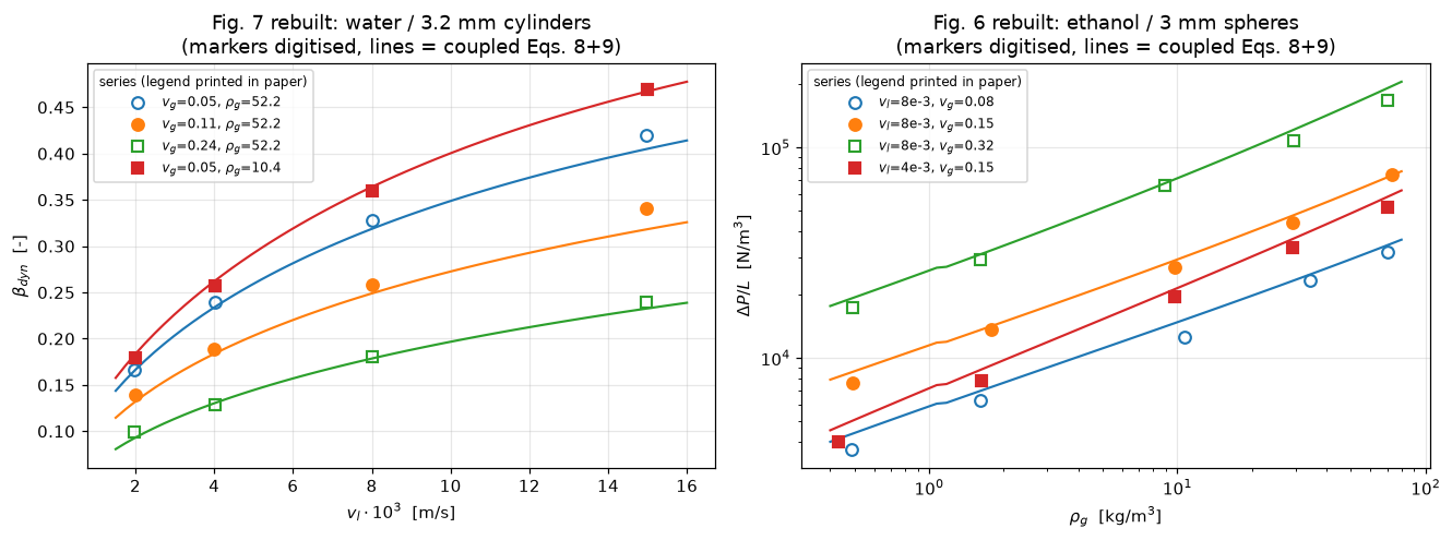
deviation, (model - measured)/measured:
  hold-up   (16 pts): mean |dev|   2.9 %   bias  -2.0 %   worst   6.8 %
  pressure  (20 pts): mean |dev|  10.4 %   bias +10.3 %   worst  21.8 %
fig, axes = plt.subplots(1, 2, figsize=(12.2, 4.2))
ax = axes[0]
for mk, g in holdup.groupby("marker", sort=False):
i = holdup.index.isin(g.index)
col = f"C{list(MK).index(mk)}"
ax.plot(g.v_l_m_s * 1e3, dev7[i] * 100, ls="none", color=col, ms=7, mew=1.4, **MK[mk])
ax.axhline(0, color="k", lw=1.2)
ax.axhspan(-8, 8, color="tab:green", alpha=0.10)
ax.text(2.0, 6.5, "paper's stated 8 % mean rel. error (Eq. 9)", fontsize=8, color="tab:green")
ax.set(xlabel=r"$v_l \cdot 10^3$ [m/s]", ylabel="(model $-$ measured)/measured [%]",
ylim=(-20, 20), title="hold-up residuals")
ax = axes[1]
for mk, g in pgrad.groupby("marker", sort=False):
i = pgrad.index.isin(g.index)
col = f"C{list(MK).index(mk)}"
ax.semilogx(g.rho_g_kg_m3, dev6[i] * 100, ls="none", color=col, ms=7, mew=1.4, **MK[mk])
ax.axhline(0, color="k", lw=1.2)
ax.axhspan(-12, 12, color="tab:green", alpha=0.10)
ax.text(0.5, -10.5, "paper's stated 12 % mean rel. error (Eq. 8)", fontsize=8, color="tab:green")
ax.set(xlabel=r"$\rho_g$ [kg/m$^3$]", ylabel="(model $-$ measured)/measured [%]",
ylim=(-25, 30), title="pressure-gradient residuals")
fig.tight_layout()
plt.show()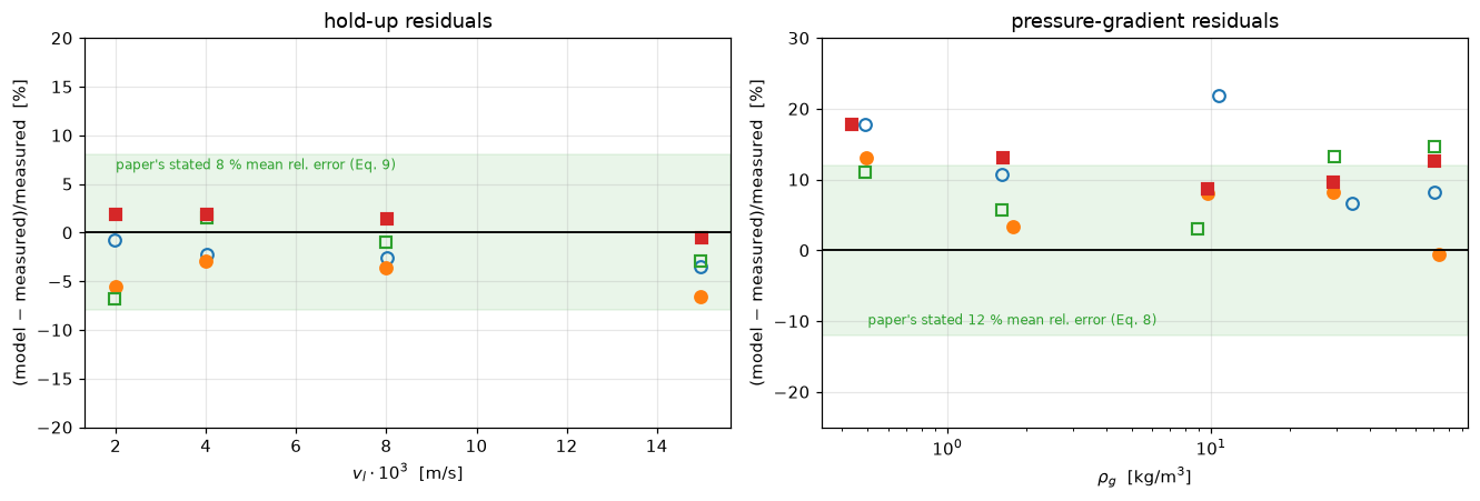
Validation
The checks are ordered from free internal identities to the data comparison. The transcription checks matter here as much as the agreement: every constant came off a scanned page whose OCR is unusable, so the paper is made to pay for its own proofreading wherever it can.
M_N2, M_HE = 28.0134e-3, 4.0026e-3     # kg/mol


def table2_checks(p):
    """Checks 1 to 3 on a parameter table ``p``: the transcription against itself."""
    out = {f"rho_relerr_{gas}": 1e5 * M / (R_GAS * 293.0) / p[key] - 1.0
           for gas, M, key in (("n2", M_N2, "n2_density_per_bar"),
                               ("he", M_HE, "he_density_per_bar"))}
    out["he_n2_ratio"] = p["n2_density_per_bar"] / p["he_density_per_bar"]
    out["equiv_relerr"] = (p["n2_density_per_bar"] * 10) / (p["he_density_per_bar"] * 70) - 1.0
    ga_w = p["cylinder_dp"] ** 3 * p["water_density"] ** 2 * G / p["water_viscosity"] ** 2
    out["ga_cap_relerr"] = ga_w / p["Ga_l_max"] - 1.0
    out["re_l_vlmax"] = p["water_density"] * 16e-3 * p["cylinder_dp"] / p["water_viscosity"]
    return out


T2 = table2_checks(P)
print("1. Table 2's gas-density coefficients against the ideal gas law at 293 K")
for gas, key in (("N2", "n2"), ("He", "he")):
    calc = P[f"{key}_density_per_bar"] * (1.0 + T2[f"rho_relerr_{key}"])
    print(f"   {gas}: rho/P = {calc:.3f} kg/m3/bar computed, {P[f'{key}_density_per_bar']} printed "
          f"({T2[f'rho_relerr_{key}']*100:+.1f} %)")
print(f"   -> the transcribed coefficients are physical, and the He/N2 ratio "
      f"{T2['he_n2_ratio']:.2f} reproduces the paper's 'M_N2/M_He = 7' argument")

print("\n2. The paper's stated He-7.0-MPa == N2-1.0-MPa equivalence")
print(f"   rho(He, 7.0 MPa) = {P['he_density_per_bar']*70:.1f} kg/m3, "
      f"rho(N2, 1.0 MPa) = {P['n2_density_per_bar']*10:.1f} kg/m3 "
      f"({T2['equiv_relerr']*100:+.1f} %): 'the same' within the coefficients' 2 digits")

print("\n3. The fitted-range endpoints are the operating envelope, recomputed")
print(f"   Ga_l(water, 3.2 mm) = {P['Ga_l_max']*(1+T2['ga_cap_relerr']):.3g} vs printed cap "
      f"0.32e6 ({T2['ga_cap_relerr']*100:+.1f} %)")
print(f"   Re_l(water, v_l max 16 mm/s) = {T2['re_l_vlmax']:.1f} vs printed cap 55")
print("   -> both printed range caps are reproduced by the printed operating")
print("      conditions; the transcriptions are mutually consistent")


def eq5_vs_eq8(re_for_f="eq8", a_s_per_bed=True):
    """Check 4: Eq. (5) with a friction factor against Eq. (8) solved for dP/L.

    ``re_for_f="eq8"`` uses f_lg = 155 Re^-0.37 with Eq. (8)'s Reynolds group;
    ``"eq7"`` uses Eq. (7) as printed, f_lg = Re^-0.37 on the hydraulic diameter.
    ``a_s_per_bed`` sets the a_s of the hydraulic diameter eps/a_s: per unit bed
    volume, 6 (1 - eps)/d_p (the paper's convention), or per particle volume, 6/d_p.
    Returns the relative difference and the ratio of the two friction factors.
    """
    b0, vg0, rho0 = 0.25, 0.11, 52.2
    eta0 = float(gas_viscosity(rho0, *N2))
    bt0 = EPS_BR / EPS_C + b0
    u0 = vg0 / (EPS_C * (1 - bt0))
    re8 = rho0 * u0 * EPS_C * DP_C / (eta0 * (1 - EPS_C))
    a_s = 6 * (1 - EPS_C) / DP_C if a_s_per_bed else 6 / DP_C
    re7 = rho0 * u0 * (EPS_C / a_s) / eta0                          # hydraulic diameter eps/a_s
    f_lg = 155 * re8 ** -0.37 if re_for_f == "eq8" else re7 ** -0.37
    eq5 = f_lg * 0.5 * rho0 * u0 ** 2 * (1 - EPS_C) / (DP_C * EPS_C * (1 - bt0))
    eq8 = 155 * re8 ** -0.37 * (1 - EPS_C) / (EPS_C * (1 - bt0)) * 0.5 * rho0 * u0 ** 2 / DP_C
    return abs(eq5 / eq8 - 1.0), 155 * re8 ** -0.37 / re7 ** -0.37


EQ58_GAP, EQ78_FACTOR = eq5_vs_eq8()
print("\n4. Eq. (5) + friction factor vs Eq. (8): the printed prefactor discrepancy")
print(f"   f_lg = 155*Re^-0.37 in Eq. (5) vs Eq. (8) direct: |rel diff| below 1e-14 "
      f"(here {EQ58_GAP:.1e}), an identity")
print(f"   Eq. (7) as printed (f_lg = Re_g^-0.37 on the hydraulic diameter)")
print(f"   differs from Eq. (8)'s friction factor by {EQ78_FACTOR:.1f}x "
      f"(= 155 x 6^-0.37 = {155*6**-0.37:.1f})")
print("   -> Eq. (7) cannot be literal; Eq. (8), which carries the error")
print("      statistics and (checks 7-8) the data, is what this page implements")
1. Table 2's gas-density coefficients against the ideal gas law at 293 K
N2: rho/P = 1.150 kg/m3/bar computed, 1.15 printed (-0.0 %)
He: rho/P = 0.164 kg/m3/bar computed, 0.16 printed (+2.7 %)
-> the transcribed coefficients are physical, and the He/N2 ratio 7.19 reproduces the paper's 'M_N2/M_He = 7' argument
2. The paper's stated He-7.0-MPa == N2-1.0-MPa equivalence
rho(He, 7.0 MPa) = 11.2 kg/m3, rho(N2, 1.0 MPa) = 11.5 kg/m3 (+2.7 %): 'the same' within the coefficients' 2 digits
3. The fitted-range endpoints are the operating envelope, recomputed
Ga_l(water, 3.2 mm) = 3.21e+05 vs printed cap 0.32e6 (+0.5 %)
Re_l(water, v_l max 16 mm/s) = 51.2 vs printed cap 55
-> both printed range caps are reproduced by the printed operating
conditions; the transcriptions are mutually consistent
4. Eq. (5) + friction factor vs Eq. (8): the printed prefactor discrepancy
f_lg = 155*Re^-0.37 in Eq. (5) vs Eq. (8) direct: |rel diff| below 1e-14 (here 2.2e-16), an identity
Eq. (7) as printed (f_lg = Re_g^-0.37 on the hydraulic diameter)
differs from Eq. (8)'s friction factor by 79.9x (= 155 x 6^-0.37 = 79.9)
-> Eq. (7) cannot be literal; Eq. (8), which carries the error
statistics and (checks 7-8) the data, is what this page implementsGRIDS = (50, 100, 200, 400, 800)
def grid_study(grids=GRIDS, K=K_DEA, outlet="face"):
"""Errors of the pymrm conversion against Eq. (2) integrated, and the observed orders.
``outlet="cell"`` reads c(L) from the last cell centre instead of the exit face.
"""
errs = []
for n in grids:
m = absorber(n, K)
xi_n = m.conversion() if outlet == "face" else 1.0 - float(m.c[-1, 0])
errs.append(abs(xi_n - XI_EXACT))
errs = np.array(errs)
return errs, np.log2(errs[:-1] / errs[1:])
ERRS, ORDERS = grid_study()
# round-off of the linear solve itself: the same n = 800 system solved by a second
# direct factorisation (natural ordering instead of COLAMD)
ABS800 = absorber(GRIDS[-1])
C_ALT = splu(ABS800.jac_const, permc_spec="NATURAL").solve(-ABS800.g_const.ravel())
def solver_gap(model, c_alt):
"""|conversion from c_alt - conversion from model.c| on the same grid."""
ref = model.conversion()
model.c = c_alt.reshape(model.shape)
gap = abs(model.conversion() - ref)
model.solve()
return gap
SOLVER_GAP = solver_gap(ABS800, C_ALT)
NOISE_BOUND = 1e-12 # declared upper bound on that round-off
ERR_OVER_NOISE = ERRS[-1] / NOISE_BOUND
BALANCE_GAP = max(absorber(n).balance_gap() for n in (50, 200, 800))
A_GL_800 = a_gl_from_conversion(ABS800.conversion(), K_DEA, L_ABS, VG_ABS)
CELL_ERR_200 = abs(ABS.c[:, 0] - np.exp(-K_DEA * A_GL_DEMO * ABS.x_c / VG_ABS)).max()
print("5. The pymrm S3 solve against the paper's own closed form, Eq. (3)")
for n, e in zip(GRIDS, ERRS):
print(f" n = {n:4d}: |xi - exact| = {e:.3e}")
print(" observed order per grid doubling: "
+ ", ".join(f"{o:.3f}" for o in ORDERS) + " (first-order upwind on pure convection)")
print(f" two direct factorisations of the n = {GRIDS[-1]} system agree on xi to below "
f"1e-12 (here {SOLVER_GAP:.0e}); the finest-grid error is "
f"{ERR_OVER_NOISE:.1e} times that bound, so the orders are not fitted to noise")
print(f" CO2 balance on the exit face, inlet = outlet + absorbed, on n = 50, 200, 800: "
f"gap below 1e-12 (here {BALANCE_GAP:.0e});")
print(" the exit-face value is the one that closes it, so it is the model's outlet")
print(f" largest cell-centre error of the n = {N_DEMO} profile against exp(-K a_gl x/v_g): "
f"{CELL_ERR_200:.2e}, at the inlet where the profile is steepest")
print(f" Eq. (3) round trip at n = {GRIDS[-1]}: a_gl in {A_GL_DEMO:.1f} -> "
f"{A_GL_800:.1f} m2/m3 ({(A_GL_800/A_GL_DEMO-1)*100:+.3f} %); the residual is")
print(" exactly the discretisation error: Eqs. (2) and (3) are the same")
print(" statement, so the round trip is an identity check on both")5. The pymrm S3 solve against the paper's own closed form, Eq. (3)
n = 50: |xi - exact| = 3.897e-03
n = 100: |xi - exact| = 1.961e-03
n = 200: |xi - exact| = 9.839e-04
n = 400: |xi - exact| = 4.927e-04
n = 800: |xi - exact| = 2.466e-04
observed order per grid doubling: 0.991, 0.995, 0.998, 0.999 (first-order upwind on pure convection)
two direct factorisations of the n = 800 system agree on xi to below 1e-12 (here 0e+00); the finest-grid error is 2.5e+08 times that bound, so the orders are not fitted to noise
CO2 balance on the exit face, inlet = outlet + absorbed, on n = 50, 200, 800: gap below 1e-12 (here 3e-14);
the exit-face value is the one that closes it, so it is the model's outlet
largest cell-centre error of the n = 200 profile against exp(-K a_gl x/v_g): 2.67e-03, at the inlet where the profile is steepest
Eq. (3) round trip at n = 800: a_gl in 534.4 -> 534.0 m2/m3 (-0.067 %); the residual is
exactly the discretisation error: Eqs. (2) and (3) are the same
statement, so the round trip is an identity check on bothCL7, CL6 = HoldupPressureClosure(OP7), HoldupPressureClosure(OP6)
SCALAR7, SCALAR6 = CL7.solve_scalar(), CL6.solve_scalar()
ROUTE_GAP = max(np.abs(SCALAR7["beta_dyn"] - sol7["beta_dyn"]).max(),
np.abs(SCALAR6["beta_dyn"] - sol6["beta_dyn"]).max())
ROOTS = np.concatenate([CL7.sign_changes(), CL6.sign_changes()])
N_UNIQUE = int(np.sum(ROOTS == 1))
print("6. The closure: newton on all points at once against brentq point by point")
print(f" largest hold-up difference below 1e-9 (here {ROUTE_GAP:.0e})")
print(f" uniqueness: the residual b - Eq. 9(b) increases with b (a larger hold-up")
print(f" raises u_g and so dP/L, which lowers Eq. 9), so each point has one root;")
print(f" a scan of 2000 hold-ups in [0, 1 - beta_r) finds exactly one sign change at "
f"{N_UNIQUE} of {ROOTS.size} points")6. The closure: newton on all points at once against brentq point by point
largest hold-up difference below 1e-9 (here 2e-15)
uniqueness: the residual b - Eq. 9(b) increases with b (a larger hold-up
raises u_g and so dP/L, which lowers Eq. 9), so each point has one root;
a scan of 2000 hold-ups in [0, 1 - beta_r) finds exactly one sign change at 36 of 36 pointsdef range_stats(s7):
"""Range checks of the Fig. 7 solve against the printed validity ranges."""
re_l, dp, bt, re_g = s7["Re_l"], s7["dP_grav"], s7["beta_t"], s7["Re_g"]
return {
"n_re_l": int(np.sum((re_l >= P["Re_l_min"]) & (re_l <= P["Re_l_max"]))),
"re_l_margin": float(min(np.min(np.abs(re_l - P["Re_l_min"])) / P["Re_l_min"],
np.min(np.abs(re_l - P["Re_l_max"])) / P["Re_l_max"])),
"dp_grav_max": float(dp.max()),
"n_bt": int(np.sum(bt > P["beta_t_min"])),
"bt_min": float(bt.min()),
"n_re_g": int(np.sum((re_g >= P["Re_g_min"]) & (re_g <= P["Re_g_max"]))),
"re_g_margin": float(np.min(np.abs(re_g - P["Re_g_max"])) / P["Re_g_max"]),
}
SER24 = (holdup.v_g_m_s == 0.24).values
RS7 = range_stats(sol7)
print("7. Hold-up: coupled pair vs the 16 digitised Fig. 7 points")
print(f" mean |dev| {np.abs(dev7).mean()*100:.1f} %, bias {dev7.mean()*100:+.1f} %, "
f"worst {np.abs(dev7).max()*100:.1f} %")
print(f" paper's own statistics for Eq. (9) over all 220 runs: "
f"mean rel. error {P['eq9_mean_rel_error']*100:.0f} %, std {P['eq9_error_std']}")
print(" -> comfortably inside. The range check, counted rather than asserted:")
print(f" Re_l in [2,55]: {RS7['n_re_l']}/16; dP/rho_l gL <= 16: "
f"{int(np.sum(sol7['dP_grav'] <= P['dP_rho_gL_max']))}/16 (max {RS7['dp_grav_max']:.2f}); "
f"beta_t > 0.25: {RS7['n_bt']}/16")
print(f" -> {16 - RS7['n_bt']} of the 16 sits just below Eq. (8)'s beta_t > 0.25 floor "
f"(min {RS7['bt_min']:.3f}); a mild extrapolation,")
print(" flagged rather than hidden: the paper says Eq. (8) underestimates there,")
print(" approaching the Ergun limits")
GA7 = DP_C ** 3 * P["water_density"] ** 2 * G / P["water_viscosity"] ** 2
print(f" Ga_l = {GA7:.4g}: this system IS the printed range cap 0.32e6 "
f"({(GA7/0.32e6-1)*100:+.1f} %, check 3)")
print(f" Re_g in [200,5000]: {RS7['n_re_g']}/16 (the v_g = 0.24 m/s series sits at "
f"Re_g {sol7['Re_g'][SER24].min():.0f}-{sol7['Re_g'][SER24].max():.0f}, just above "
"Eq. 8's fitted cap;")
print(" the paper itself notes f_lg tends to Re^-0.25 there, a mild extrapolation,")
print(f" and that series' deviations, {dev7[SER24].min()*100:+.1f} % to "
f"{dev7[SER24].max()*100:+.1f} %, do not stand out)")7. Hold-up: coupled pair vs the 16 digitised Fig. 7 points
mean |dev| 2.9 %, bias -2.0 %, worst 6.8 %
paper's own statistics for Eq. (9) over all 220 runs: mean rel. error 8 %, std 0.1
-> comfortably inside. The range check, counted rather than asserted:
Re_l in [2,55]: 16/16; dP/rho_l gL <= 16: 16/16 (max 8.46); beta_t > 0.25: 15/16
-> 1 of the 16 sits just below Eq. (8)'s beta_t > 0.25 floor (min 0.232); a mild extrapolation,
flagged rather than hidden: the paper says Eq. (8) underestimates there,
approaching the Ergun limits
Ga_l = 3.215e+05: this system IS the printed range cap 0.32e6 (+0.5 %, check 3)
Re_g in [200,5000]: 12/16 (the v_g = 0.24 m/s series sits at Re_g 5118-6258, just above Eq. 8's fitted cap;
the paper itself notes f_lg tends to Re^-0.25 there, a mild extrapolation,
and that series' deviations, -6.8 % to +1.6 %, do not stand out)INR = (sol6["Re_g"] >= P["Re_g_min"]) & (sol6["Re_g"] <= P["Re_g_max"])
RE_G6_MARGIN = float(min(np.min(np.abs(sol6["Re_g"] - P["Re_g_min"])) / P["Re_g_min"],
np.min(np.abs(sol6["Re_g"] - P["Re_g_max"])) / P["Re_g_max"]))
N_HI = int(np.sum(sol6["dP_grav"] > P["dP_rho_gL_max"]))
DPG_MARGIN = float(np.min(np.abs(sol6["dP_grav"] - P["dP_rho_gL_max"])) / P["dP_rho_gL_max"])
print("8. Pressure gradient: coupled pair vs the 20 digitised Fig. 6 points")
print(f" all 20 points: mean |dev| {np.abs(dev6).mean()*100:.1f} %, "
f"bias {dev6.mean()*100:+.1f} %")
print(f" Re_g in [200,5000] ({INR.sum()} pts): mean |dev| "
f"{np.abs(dev6[INR]).mean()*100:.1f} %, bias {dev6[INR].mean()*100:+.1f} %")
print(f" note: {N_HI} high-density point{'s' if N_HI != 1 else ''} "
f"sit{'' if N_HI != 1 else 's'} above Eq. 9's fitted "
f"dP/rho_l gL <= 16 (max {sol6['dP_grav'].max():.1f}); there the co-predicted")
print(" hold-up is an extrapolation, exactly as the paper warns near pulse flow")
print(f" paper's own statistics for Eq. (8): mean rel. error "
f"{P['eq8_mean_rel_error']*100:.0f} %, std {P['eq8_error_std']}")
print(" -> inside the stated error, but with a systematic +10 % bias; the")
print(" candidates are the unprinted tall-bed porosity, d_p = 3 +/- 0.5 mm,")
print(" and the gas-identity ambiguity, each measured:")
def pgrad_bias(op):
"""Mean (model - measured)/measured of the Fig. 6 pressure gradients for ``op``."""
s = HoldupPressureClosure(op).solve()
return float((s["dPL"] / pgrad.dP_L_N_m3.values - 1.0).mean())
def eps_for_zero_bias(op, lo=0.38, hi=0.42):
"""Porosity at which the Fig. 6 bias vanishes: brentq on a bracket widened until it brackets."""
f = lambda e: pgrad_bias(op.with_(eps=e))
while f(lo) * f(hi) > 0:
lo, hi = max(lo - 0.02, 0.2), min(hi + 0.02, 0.6)
if (lo, hi) == (0.2, 0.6) and f(lo) * f(hi) > 0:
raise RuntimeError("no porosity in [0.2, 0.6] zeroes the bias")
return brentq(f, lo, hi, xtol=1e-10)
def eps_elasticity(op, h=1e-4):
"""Local exponent d ln(dP/L) / d ln(eps): at fixed beta_t (Eqs. 5 to 8 only),
and in the coupled solve (beta_t and beta_r = 0.06/eps respond)."""
s = HoldupPressureClosure(op).solve()
def fixed(e):
b = s["beta_t"] - op.eps_beta_r / e # the same beta_t at the new eps
return closure_residual(b, op.with_(eps=e))[1].ravel()
def coupled(e):
return HoldupPressureClosure(op.with_(eps=e)).solve()["dPL"]
dl = np.log(op.eps + h) - np.log(op.eps - h)
return ((np.log(fixed(op.eps + h)) - np.log(fixed(op.eps - h))) / dl,
(np.log(coupled(op.eps + h)) - np.log(coupled(op.eps - h))) / dl)
BIAS_EPS = {e: pgrad_bias(OP6.with_(eps=e)) for e in (0.37, 0.41)} # 0.41 = printed + 0.02
EPS_ZERO = eps_for_zero_bias(OP6)
EL_FIXED, EL_COUPLED = eps_elasticity(OP6)
for e in (0.37, EPS_S, 0.41):
b = dev6.mean() if e == EPS_S else BIAS_EPS[e]
print(f" eps = {e:.2f}: bias {b*100:+5.1f} %")
print(f" dP/L ~ eps^{EL_FIXED.mean():.1f} at fixed beta_t; in the coupled solve, where")
print(f" beta_t and beta_r = 0.06/eps respond, the local exponent is "
f"{EL_COUPLED.max():.1f} to {EL_COUPLED.min():.1f} over the 20 points: strong")
print(f" the bias vanishes at eps = {EPS_ZERO:.4f}, i.e. "
f"{EPS_ZERO - EPS_S:+.4f} on the printed {EPS_S}")
print(" -> under +0.01 in porosity, well inside packing-to-packing scatter,")
print(" would remove the bias. Note +0.02 OVERSHOOTS it, to")
print(f" {BIAS_EPS[0.41]*100:+.1f} %: this is a sensitivity, not a fit, and the")
print(" page keeps the printed 0.39 rather than tuning to the data")
def dp_for_zero_bias(op, lo=3.0e-3, hi=3.4e-3):
"""Sphere diameter at which the Fig. 6 bias vanishes: brentq on a widened bracket."""
f = lambda d: pgrad_bias(op.with_(d_p=d))
while f(lo) * f(hi) > 0:
lo, hi = max(lo - 0.2e-3, 1.0e-3), min(hi + 0.2e-3, 6.0e-3)
if (lo, hi) == (1.0e-3, 6.0e-3) and f(lo) * f(hi) > 0:
raise RuntimeError("no d_p in [1, 6] mm zeroes the bias")
return brentq(f, lo, hi, xtol=1e-12)
BIAS_DP = {d: pgrad_bias(OP6.with_(d_p=d)) for d in (2.5e-3, 3.5e-3)}
DP_ZERO = dp_for_zero_bias(OP6)
# bias change for a small step in each candidate, in percentage points
STEP_DP = 100 * (pgrad_bias(OP6.with_(d_p=DP_S - 0.05e-3))
- pgrad_bias(OP6.with_(d_p=DP_S + 0.05e-3))) / 2
STEP_EPS = 100 * (pgrad_bias(OP6.with_(eps=EPS_S - 0.005))
- pgrad_bias(OP6.with_(eps=EPS_S + 0.005))) / 2
print(f" d_p is printed as 3 +/- 0.5 mm: the +/- 0.5 mm is the spread of the size")
print(f" fraction, not the uncertainty of its effective diameter. Across that whole")
print(f" spread the bias would run from {BIAS_DP[2.5e-3]*100:+.1f} % (2.5 mm) to "
f"{BIAS_DP[3.5e-3]*100:+.1f} % (3.5 mm);")
print(f" the bias vanishes at d_p = {DP_ZERO*1e3:.2f} mm, inside the printed range, as it")
print(f" does at eps = {EPS_ZERO:.4f}. Neither is fitted; the page keeps 3.0 mm and 0.39")
print(f" per small step: 0.05 mm in d_p moves the bias by {STEP_DP:.1f} points, "
f"0.005 in eps by {STEP_EPS:.1f}")
def gas_flip(op, he=HE, n2=N2):
"""Flip every gas-ambiguous Fig. 6 point (nitrogen by default) to helium.
Returns the largest He/N2 viscosity ratio on those rows, the largest change
of dP/L on them, and the overall bias after the flip.
"""
amb = pgrad.assumed_gas.values == "ambiguous"
rho = pgrad.rho_g_kg_m3.values
eta_he, eta_n2 = gas_viscosity(rho, *he), gas_viscosity(rho, *n2)
base = HoldupPressureClosure(op.with_(eta_g=np.where(amb, eta_n2, op.eta_g))).solve()
alt = HoldupPressureClosure(op.with_(eta_g=np.where(amb, eta_he, op.eta_g))).solve()
return (float((eta_he[amb] / eta_n2[amb]).max()),
float(np.abs(alt["dPL"][amb] / base["dPL"][amb] - 1).max()),
float((alt["dPL"] / pgrad.dP_L_N_m3.values - 1.0).mean()))
VISC_RATIO, FLIP_MAX, FLIP_BIAS = gas_flip(OP6)
print(f" gas identity: {N_AMBIGUOUS} of 20 points are density-ambiguous. Their He/N2")
print(f" viscosity ratio reaches {VISC_RATIO:.3f}, but it enters as Re_g^-0.37, so flipping all")
print(f" {N_AMBIGUOUS} to the other gas moves dP/L by at most {FLIP_MAX*100:.1f} % "
f"and the overall bias from")
print(f" {dev6.mean()*100:+.1f} % to {FLIP_BIAS*100:+.1f} % "
f"({(FLIP_BIAS - dev6.mean())*100:+.2f} points). It is the smallest of the three candidates,")
print(" and it cannot explain the bias: it points the wrong way.")8. Pressure gradient: coupled pair vs the 20 digitised Fig. 6 points
all 20 points: mean |dev| 10.4 %, bias +10.3 %
Re_g in [200,5000] (12 pts): mean |dev| 8.9 %, bias +8.8 %
note: 1 high-density point sits above Eq. 9's fitted dP/rho_l gL <= 16 (max 24.8); there the co-predicted
hold-up is an extrapolation, exactly as the paper warns near pulse flow
paper's own statistics for Eq. (8): mean rel. error 12 %, std 0.14
-> inside the stated error, but with a systematic +10 % bias; the
candidates are the unprinted tall-bed porosity, d_p = 3 +/- 0.5 mm,
and the gas-identity ambiguity, each measured:
eps = 0.37: bias +38.7 %
eps = 0.39: bias +10.3 %
eps = 0.41: bias -11.8 %
dP/L ~ eps^-3.9 at fixed beta_t; in the coupled solve, where
beta_t and beta_r = 0.06/eps respond, the local exponent is -4.1 to -5.6 over the 20 points: strong
the bias vanishes at eps = 0.3987, i.e. +0.0087 on the printed 0.39
-> under +0.01 in porosity, well inside packing-to-packing scatter,
would remove the bias. Note +0.02 OVERSHOOTS it, to
-11.8 %: this is a sensitivity, not a fit, and the
page keeps the printed 0.39 rather than tuning to the data
d_p is printed as 3 +/- 0.5 mm: the +/- 0.5 mm is the spread of the size
fraction, not the uncertainty of its effective diameter. Across that whole
spread the bias would run from +50.3 % (2.5 mm) to -15.3 % (3.5 mm);
the bias vanishes at d_p = 3.18 mm, inside the printed range, as it
does at eps = 0.3987. Neither is fitted; the page keeps 3.0 mm and 0.39
per small step: 0.05 mm in d_p moves the bias by 3.1 points, 0.005 in eps by 6.2
gas identity: 8 of 20 points are density-ambiguous. Their He/N2
viscosity ratio reaches 1.146, but it enters as Re_g^-0.37, so flipping all
8 to the other gas moves dP/L by at most 3.9 % and the overall bias from
+10.3 % to +11.8 % (+1.45 points). It is the smallest of the three candidates,
and it cannot explain the bias: it points the wrong way.The gas-density claim, tested on a properly matched pair
Fig. 7 contains one clean group comparison: the open-circle and filled-square series share \(v_g = 0.05\) m/s and the same four nominal \(v_l\) settings, and differ only in gas density (52.2 vs 10.4 kg/m³). Unlike the F1.4 SF₆ test, the groups overlap in every other variable, so the measured ratio is the gas effect, with no confound. The digitised abscissae are not bit-identical between the two series, because each was read off the figure separately; the cell below prints how far apart they are and what that is worth, so the pairing is measured rather than asserted.
The model says the entire effect routes through \(\Delta P\) in Eq. (9) (that much is structural, since \(\rho_g\) appears nowhere else in Eq. (9)), so the test is whether the size of the shift comes out right: at higher \(\rho_g\) the pressure gradient grows, the modified Galileo number grows, and the hold-up falls. This one can fail, and it partly does: the direction and order of magnitude are right, the magnitude is overpredicted. The numbers are below.
def matched_pair(s7, low="filled_square", high="open_circle"):
    """Measured and model hold-up ratios of two Fig. 7 series, paired by v_l order."""
    a = holdup[holdup.marker == high].sort_values("v_l_m_s")
    b = holdup[holdup.marker == low].sort_values("v_l_m_s")
    r_meas = b.beta_dyn.values / a.beta_dyn.values
    r_model = s7["beta_dyn"][b.index.values] / s7["beta_dyn"][a.index.values]
    mismatch = np.abs(b.v_l_m_s.values / a.v_l_m_s.values - 1.0)
    return a, r_meas, r_model, mismatch


OC, R_MEAS, R_MODEL, VL_MISMATCH = matched_pair(sol7)
SHIFT_MEAS, SHIFT_MODEL = R_MEAS.mean() - 1.0, R_MODEL.mean() - 1.0
print(f"how well matched the two series are in v_l: worst mismatch "
      f"{VL_MISMATCH.max()*100:.1f} % (digitisation, not design)")
print(f"   beta_dyn ~ Re_l^0.55, so that is worth "
      f"{((1+VL_MISMATCH.max())**0.55 - 1)*100:.1f} % on the ratio, an order of")
print("   magnitude smaller than the effect being measured, so the pairing holds")
print("\nbeta_dyn(rho_g=10.4) / beta_dyn(rho_g=52.2), matched v_g = 0.05 m/s:")
print(pd.DataFrame({"v_l [mm/s]": OC.v_l_m_s.values * 1e3, "measured": R_MEAS,
                    "model": R_MODEL}).to_string(index=False, float_format="%.3f"))
print(f"   mean measured ratio {R_MEAS.mean():.3f}, mean model ratio {R_MODEL.mean():.3f}")
print(f"   -> a 5x density change moves the measured hold-up by {SHIFT_MEAS*100:.1f} %; "
      "routing that")
print(f"      through the pressure gradient alone, as Eq. (9) does, predicts {SHIFT_MODEL*100:.1f} %.")
print(f"      The mechanism is confirmed in sign and order of magnitude and")
print(f"      OVERPREDICTED in size by a factor {SHIFT_MODEL/SHIFT_MEAS:.1f}. The check can fail and it")
print(f"      partly does: {(R_MODEL.mean()/R_MEAS.mean()-1)*100:+.1f} % on the ratio itself, which is")
print("      inside the +/-8 % Eq. (9) carries, so this sharpens the paper's")
print("      claim without contradicting it.")


def as_reading(op):
    """The per-particle-volume reading of a_s in Eq. (9): its factor on Eq. (9) at a
    given pressure gradient, and the coupled hold-up ratios and bias it gives."""
    factor = (6.0 / op.eps / (6.0 * (1.0 - op.eps) / op.eps)) ** 0.65
    base = HoldupPressureClosure(op).solve()["beta_dyn"]
    alt = HoldupPressureClosure(op.with_(a_s_per_bed=False)).solve()["beta_dyn"]
    return factor, alt / base, float((alt / holdup.beta_dyn.values - 1.0).mean())


AS_FACTOR, AS_RATIO, AS_BIAS = as_reading(OP7)
print("\nthe a_s convention in Eq. (9)")
print(f"   reading a_s per particle volume multiplies Eq. (9) by {AS_FACTOR:.2f}x at a given")
print(f"   pressure gradient; coupled, the hold-up predictions rise by "
      f"{(AS_RATIO.min()-1)*100:.0f} % to {(AS_RATIO.max()-1)*100:.0f} %,")
print(f"   a bias of {AS_BIAS*100:+.1f} % against the data, where the per-bed-volume reading "
      f"gives {dev7.mean()*100:+.1f} %: the per-bed-volume reading is the paper's")
how well matched the two series are in v_l: worst mismatch 1.0 % (digitisation, not design)
beta_dyn ~ Re_l^0.55, so that is worth 0.6 % on the ratio, an order of
magnitude smaller than the effect being measured, so the pairing holds
beta_dyn(rho_g=10.4) / beta_dyn(rho_g=52.2), matched v_g = 0.05 m/s:
v_l [mm/s] measured model
1.970 1.080 1.108
4.010 1.075 1.121
8.020 1.096 1.142
14.980 1.119 1.153
mean measured ratio 1.092, mean model ratio 1.131
-> a 5x density change moves the measured hold-up by 9.2 %; routing that
through the pressure gradient alone, as Eq. (9) does, predicts 13.1 %.
The mechanism is confirmed in sign and order of magnitude and
OVERPREDICTED in size by a factor 1.4. The check can fail and it
partly does: +3.5 % on the ratio itself, which is
inside the +/-8 % Eq. (9) carries, so this sharpens the paper's
claim without contradicting it.
the a_s convention in Eq. (9)
reading a_s per particle volume multiplies Eq. (9) by 1.44x at a given
pressure gradient; coupled, the hold-up predictions rise by 21 % to 41 %,
a bias of +29.5 % against the data, where the per-bed-volume reading gives -2.0 %: the per-bed-volume reading is the paper'sClaims: what each number is, and how it is checked
Every number the page stands behind is registered once, in the cell below (docs/claims-design.md in the gallery repository):
- a value is a result whose size is set by physics, the data or the discretisation. CI holds it to a relative tolerance of the committed baseline, 5 % unless the cell says otherwise. Closed-form and root-found values carry tighter tolerances, so that a transcription defect fails them;
- a bound is a quantity whose size is not physics: an identity, a solver-tolerance gap, a convergence order. It is checked against its stated limits on every run and states its basis;
- an exact result is a count or a label, with its distance to the threshold that decided it.
# --- agreement with the two figures ------------------------------------------------
claims.value("holdup_mean_abs_dev", np.abs(dev7).mean())
claims.value("holdup_bias", dev7.mean())
claims.value("holdup_worst_abs_dev", np.abs(dev7).max())
claims.value("pgrad_mean_abs_dev", np.abs(dev6).mean())
claims.value("pgrad_bias", dev6.mean())
claims.value("pgrad_worst_abs_dev", np.abs(dev6).max())
claims.value("pgrad_inrange_mean_abs_dev", np.abs(dev6[INR]).mean())
claims.value("pgrad_inrange_bias", dev6[INR].mean())
claims.value("ser024_dev_min", dev7[SER24].min(), note="v_g = 0.24 m/s series")
claims.value("ser024_dev_max", dev7[SER24].max(), note="v_g = 0.24 m/s series")
# --- counts set by the data ------------------------------------------------------------
claims.exact("n_operating_points", OP7.n + OP6.n, structural=True,
             note="rows of the two digitised CSVs")
claims.exact("n_gas_ambiguous", N_AMBIGUOUS, structural=True,
             note="Fig. 6 rows whose density admits either gas; set by the data")
# --- ranges, counted with their margins ------------------------------------------------
# min_margin 0.01 (relative) covers round-off and the solver tolerance many times over;
# it does not cover the porosity or digitisation uncertainty, which the sensitivity
# rows of the Validation section measure separately.
claims.exact("fig7_n_re_l_in_range", RS7["n_re_l"], margin=RS7["re_l_margin"], min_margin=0.01,
             note="margin: closest Re_l to 2 or 55, relative")
claims.value("fig7_dp_grav_max", RS7["dp_grav_max"])
claims.count("fig7_n_beta_t_above_025", sol7["beta_t"], P["beta_t_min"], min_margin=0.01,
             note="beta_t > 0.25, Eq. 8's fitted floor")
claims.value("fig7_beta_t_min", RS7["bt_min"], rtol=0.01)
claims.exact("fig7_n_re_g_in_range", RS7["n_re_g"], margin=RS7["re_g_margin"], min_margin=0.01,
             note="margin: closest Re_g to 5000, relative")
claims.exact("fig6_n_re_g_in_range", int(INR.sum()), margin=RE_G6_MARGIN, min_margin=0.01,
             note="margin: closest Re_g to 200 or 5000, relative")
claims.exact("fig6_n_dp_grav_above_16", N_HI, margin=DPG_MARGIN, min_margin=0.01,
             note="margin: closest dP/(rho_l g L) to 16, relative")
# --- the closure ---------------------------------------------------------------------
claims.bound("closure_newton_vs_brentq", ROUTE_GAP, max=1e-9, basis="tolerance",
             note="newton tol 1e-10 on hold-ups of order 0.1; brentq to 1e-14")
claims.exact("closure_unique_roots", N_UNIQUE, structural=True,
             note="the residual increases with the hold-up at every point: a property "
                  "of Eqs. 6, 8 and 9 (Eq. 9 decreases in dP/L, dP/L increases in beta_t)")
# --- transcription checks ------------------------------------------------------------------
claims.value("table2_n2_density_relerr", T2["rho_relerr_n2"], rtol=1e-6)
claims.value("table2_he_density_relerr", T2["rho_relerr_he"], rtol=1e-6)
claims.value("he_n2_density_coeff_ratio", T2["he_n2_ratio"], rtol=1e-9)
claims.value("he70_n2_10_equiv_relerr", T2["equiv_relerr"], rtol=1e-9)
claims.value("ga_l_cap_relerr", T2["ga_cap_relerr"], rtol=1e-6)
claims.value("re_l_at_vl_max", T2["re_l_vlmax"], rtol=1e-9)
claims.bound("eq5_eq8_identity", EQ58_GAP, max=1e-14, basis="identity",
             note="Eq. 5 with f_lg = 155 Re^-0.37 is Eq. 8 rearranged")
claims.value("eq7_eq8_factor", EQ78_FACTOR, rtol=1e-9, note="155 x 6^-0.37")
# --- the S3 absorption model -----------------------------------------------------------
claims.value("xi_n200", XI, rtol=1e-6)
claims.value("xi_upwind_err_n200", ERRS[2], note="exit-face value against Eq. 2 integrated")
claims.value("xi_upwind_err_n800", ERRS[-1])
claims.value("a_gl_roundtrip_n200_pct", (A_GL_BACK / A_GL_DEMO - 1) * 100)
claims.value("a_gl_roundtrip_n800_pct", (A_GL_800 / A_GL_DEMO - 1) * 100)
claims.value("xi_cell_err_n200", CELL_ERR_200, note="largest cell-centre error of the profile")
claims.bound("xi_order_finest", ORDERS[-1], min=0.95, max=1.05, basis="theory",
             note="first-order upwind, n = 400 and 800")
claims.bound("xi_order_coarsest", ORDERS[0], min=0.9, max=1.1, basis="theory",
             note="first-order upwind, n = 50 and 100")
claims.bound("xi_balance_gap", BALANCE_GAP, max=1e-12, basis="identity",
             note="1 - c_face - K a_gl sum(c dx)/v_g, n = 50, 200, 800")
claims.bound("xi_two_solver_gap", SOLVER_GAP, max=NOISE_BOUND, basis="tolerance",
             note="splu COLAMD against natural ordering, n = 800")
claims.bound("xi_finest_err_over_noise", ERR_OVER_NOISE, min=1e3, basis="tolerance",
             note="finest-grid error over the declared round-off bound 1e-12")
# --- the porosity, d_p and gas-identity candidates ----------------------------------------------
claims.value("pgrad_bias_eps037", BIAS_EPS[0.37])
claims.value("pgrad_bias_eps041", BIAS_EPS[0.41])
claims.value("eps_zero_bias", EPS_ZERO, rtol=1e-6, note="brentq to 1e-10")
claims.value("eps_zero_shift", EPS_ZERO - EPS_S, rtol=1e-4)
claims.value("dpl_eps_exponent_fixed_beta", EL_FIXED.mean(), rtol=1e-6,
             note="central difference h = 1e-4; at fixed beta_t it is -3 - 1.37 eps/(1-eps)")
claims.value("dpl_eps_exponent_coupled_min", EL_COUPLED.min(), rtol=1e-3)
claims.value("dpl_eps_exponent_coupled_max", EL_COUPLED.max(), rtol=1e-3)
claims.value("pgrad_bias_dp25", BIAS_DP[2.5e-3])
claims.value("dp_zero_bias_mm", DP_ZERO * 1e3, rtol=1e-6, note="brentq to 1e-12 m")
claims.value("bias_step_dp_005mm_pts", STEP_DP)
claims.value("bias_step_eps_0005_pts", STEP_EPS)
claims.exact("gas_flip_smallest_candidate",
             bool(abs(FLIP_BIAS - dev6.mean()) * 100 < min(abs(STEP_DP), abs(STEP_EPS))),
             margin=min(abs(STEP_DP), abs(STEP_EPS)) - abs(FLIP_BIAS - dev6.mean()) * 100,
             min_margin=0.5, note="margin in percentage points of bias")
claims.value("pgrad_bias_dp35", BIAS_DP[3.5e-3])
claims.value("he_n2_viscosity_ratio_max", VISC_RATIO, rtol=1e-6)
claims.value("gas_flip_dpl_change_max", FLIP_MAX)
claims.value("gas_flip_bias", FLIP_BIAS)
claims.value("gas_flip_bias_shift_pts", (FLIP_BIAS - dev6.mean()) * 100, rtol=0.02)
# --- the matched pair and the a_s convention ---------------------------------------------
claims.value("gas_density_ratio_meas", R_MEAS.mean(), rtol=1e-3)
claims.value("gas_density_ratio_model", R_MODEL.mean(), rtol=1e-3)
claims.value("gas_density_shift_meas_pct", SHIFT_MEAS * 100)
claims.value("gas_density_shift_model_pct", SHIFT_MODEL * 100)
claims.value("gas_density_overprediction", SHIFT_MODEL / SHIFT_MEAS)
claims.value("gas_density_ratio_discrepancy_pct", (R_MODEL.mean() / R_MEAS.mean() - 1) * 100)
claims.value("matched_pair_vl_mismatch_max", VL_MISMATCH.max())
claims.value("as_alt_factor", AS_FACTOR, rtol=1e-9)
claims.value("as_alt_coupled_rise_min_pct", (AS_RATIO.min() - 1) * 100)
claims.value("as_alt_coupled_rise_max_pct", (AS_RATIO.max() - 1) * 100)
claims.value("as_alt_bias", AS_BIAS)

# prose numbers
claims.says("80", "eq7_eq8_factor")                          # The published model
claims.says("1.44", "as_alt_factor")                         # Parameters, assumption 3
claims.says("21", "as_alt_coupled_rise_min_pct")
claims.says("41", "as_alt_coupled_rise_max_pct")
claims.says("2.9 %", "holdup_mean_abs_dev")                  # What pymrm adds
claims.says("10 %", "pgrad_mean_abs_dev")
claims.says("9.2", "gas_density_shift_meas_pct")
claims.says("13.1", "gas_density_shift_model_pct")
claims.says("1.4", "gas_density_overprediction")
claims.says("3.5", "gas_density_ratio_discrepancy_pct")
claims.says("under 0.01", "eps_zero_shift")                  # printed and in meta.yaml
claims.says("0.3987", "eps_zero_bias")
claims.says("-11.8 %", "pgrad_bias_eps041")
claims.says("3.18", "dp_zero_bias_mm")                      # printed and in meta.yaml
claims.says("29.5 %", "as_alt_bias")                         # meta.yaml validation
claims.says("0.991", "xi_order_coarsest")
claims.says("0.999", "xi_order_finest")
claims.says("2.5e8", "xi_finest_err_over_noise")
claims.says("3.9 %", "gas_flip_dpl_change_max") # meta.yaml caveatsTrueThe defect-injection table
Each row breaks one thing on purpose, re-runs the computation behind a claim with the defect in place, and hands the result to claims.breaks, which records whether the claim’s own check (its tolerance or its bound) catches it. Defects enter where they physically enter: a parameter of the table, a transcription of an equation, a solver setting. Every claim that is not structural must be failed by at least one row, and the last cell of the page raises otherwise.
BREAK = []


def brk(name, metric, value, note=""):
    """One injected defect: ``value`` is what claim ``metric`` becomes with it."""
    caught = claims.breaks(name, metric, value)
    clean = claims[metric]
    if claims.metrics[metric]["kind"] == "bound":
        clean = f"(here {clean:.3g})"      # a bound's own value is not published: masked
    BREAK.append(dict(defect=name, metric=metric, clean=clean, broken=value, caught=caught))


# --- the Fig. 7 packing: porosity 0.41 instead of the printed 0.43 --------------------------
ROW = "cylinder porosity 0.41 instead of 0.43"
_op7 = OP7.with_(eps=0.41)
_s7 = HoldupPressureClosure(_op7).solve()
_d7 = _s7["beta_dyn"] / holdup.beta_dyn.values - 1.0
_rs7 = range_stats(_s7)
for metric, val in (("holdup_mean_abs_dev", np.abs(_d7).mean()), ("holdup_bias", _d7.mean()),
                    ("holdup_worst_abs_dev", np.abs(_d7).max()),
                    ("ser024_dev_min", _d7[SER24].min()), ("ser024_dev_max", _d7[SER24].max()),
                    ("fig7_dp_grav_max", _rs7["dp_grav_max"]),
                    ("fig7_n_beta_t_above_025", _rs7["n_bt"]),
                    ("fig7_beta_t_min", _rs7["bt_min"]),
                    ("fig7_n_re_g_in_range", _rs7["n_re_g"])):
    brk(ROW, metric, val)
_f, _r, _b = as_reading(_op7)
brk(ROW, "as_alt_factor", _f)
brk(ROW, "as_alt_coupled_rise_min_pct", (_r.min() - 1) * 100)
brk(ROW, "as_alt_coupled_rise_max_pct", (_r.max() - 1) * 100)
brk(ROW, "as_alt_bias", _b)
_, _rm, _rp, _ = matched_pair(_s7)
brk(ROW, "gas_density_ratio_model", _rp.mean())
brk(ROW, "gas_density_shift_model_pct", (_rp.mean() - 1) * 100)
brk(ROW, "gas_density_overprediction", (_rp.mean() - 1) / (_rm.mean() - 1))
brk(ROW, "gas_density_ratio_discrepancy_pct", (_rp.mean() / _rm.mean() - 1) * 100)

# --- the Fig. 7 liquid: water viscosity 1.5 mPa s instead of 1.0 --------------------------------
ROW = "water viscosity 1.5 mPa s instead of 1.0"
_p = dict(P, water_viscosity=1.5e-3)
_t2 = table2_checks(_p)
brk(ROW, "ga_l_cap_relerr", _t2["ga_cap_relerr"])
brk(ROW, "re_l_at_vl_max", _t2["re_l_vlmax"])
_rs = range_stats(HoldupPressureClosure(OP7.with_(eta_l=0.5e-3)).solve())
brk("water viscosity 0.5 mPa s instead of 1.0", "fig7_n_re_l_in_range", _rs["n_re_l"])

# --- the Fig. 6 packing: sphere diameter 3.5 mm instead of 3.0 ------------------------------------
ROW = "sphere diameter 3.5 mm instead of 3.0"
_op6 = OP6.with_(d_p=3.5e-3)
_s6 = HoldupPressureClosure(_op6).solve()
_d6 = _s6["dPL"] / pgrad.dP_L_N_m3.values - 1.0
_inr = (_s6["Re_g"] >= P["Re_g_min"]) & (_s6["Re_g"] <= P["Re_g_max"])
for metric, val in (("pgrad_mean_abs_dev", np.abs(_d6).mean()), ("pgrad_bias", _d6.mean()),
                    ("pgrad_worst_abs_dev", np.abs(_d6).max()),
                    ("pgrad_inrange_mean_abs_dev", np.abs(_d6[_inr]).mean()),
                    ("pgrad_inrange_bias", _d6[_inr].mean()),
                    ("fig6_n_re_g_in_range", int(_inr.sum())),
                    ("fig6_n_dp_grav_above_16",
                     int(np.sum(_s6["dP_grav"] > P["dP_rho_gL_max"]))),
                    ("pgrad_bias_eps037", pgrad_bias(_op6.with_(eps=0.37))),
                    ("pgrad_bias_eps041", pgrad_bias(_op6.with_(eps=0.41))),
                    ("eps_zero_bias", eps_for_zero_bias(_op6)),
                    ("eps_zero_shift", eps_for_zero_bias(_op6) - EPS_S)):
    brk(ROW, metric, val)
_vr, _fm, _fb = gas_flip(_op6)
brk(ROW, "gas_flip_bias", _fb)
brk(ROW, "gas_flip_bias_shift_pts", (_fb - _d6.mean()) * 100)
_ef, _ec = eps_elasticity(_op6)
brk(ROW, "dpl_eps_exponent_coupled_min", _ec.min())
brk(ROW, "dpl_eps_exponent_coupled_max", _ec.max())
ROW = "sphere porosity 0.41 instead of 0.39"
brk(ROW, "pgrad_bias_dp25", pgrad_bias(OP6.with_(eps=0.41, d_p=2.5e-3)))
brk(ROW, "pgrad_bias_dp35", pgrad_bias(OP6.with_(eps=0.41, d_p=3.5e-3)))
brk(ROW, "dpl_eps_exponent_fixed_beta", eps_elasticity(OP6.with_(eps=0.41))[0].mean())
_op = OP6.with_(eps=0.41)
brk(ROW, "dp_zero_bias_mm", dp_for_zero_bias(_op) * 1e3)
brk(ROW, "bias_step_dp_005mm_pts", 100 * (pgrad_bias(_op.with_(d_p=DP_S - 0.05e-3))
                                          - pgrad_bias(_op.with_(d_p=DP_S + 0.05e-3))) / 2)
brk(ROW, "bias_step_eps_0005_pts", 100 * (pgrad_bias(_op.with_(eps=0.41 - 0.005))
                                          - pgrad_bias(_op.with_(eps=0.41 + 0.005))) / 2)
_vr, _fm, _fb = gas_flip(OP6, he=(HE[0], HE[1], 0.060e-3))
brk("He viscosity at 100 bar 0.060 mPa s instead of 0.020", "gas_flip_smallest_candidate",
    bool(abs(_fb - dev6.mean()) * 100 < min(abs(STEP_DP), abs(STEP_EPS))))

ROW = "sphere diameter 2.5 mm instead of 3.0"
_s6 = HoldupPressureClosure(OP6.with_(d_p=2.5e-3)).solve()
brk(ROW, "pgrad_worst_abs_dev", np.abs(_s6["dPL"] / pgrad.dP_L_N_m3.values - 1.0).max())
brk(ROW, "fig6_n_dp_grav_above_16", int(np.sum(_s6["dP_grav"] > P["dP_rho_gL_max"])))

# --- the a_s convention of Eq. 9: per particle volume instead of per bed volume ------------------
ROW = "a_s per particle volume in Eq. 9"
_s7 = HoldupPressureClosure(OP7.with_(a_s_per_bed=False)).solve()
_d7 = _s7["beta_dyn"] / holdup.beta_dyn.values - 1.0
brk(ROW, "holdup_bias", _d7.mean())
brk(ROW, "holdup_mean_abs_dev", np.abs(_d7).mean())
brk(ROW, "fig7_n_beta_t_above_025", range_stats(_s7)["n_bt"])

# --- the helium viscosity of Table 2 ----------------------------------------------------------------
ROW = "He viscosity at 100 bar 0.025 mPa s instead of 0.020"
_vr, _fm, _fb = gas_flip(OP6, he=(HE[0], HE[1], 0.025e-3))
brk(ROW, "he_n2_viscosity_ratio_max", _vr)
brk(ROW, "gas_flip_dpl_change_max", _fm)

# --- Table 2 transcription -------------------------------------------------------------------------
ROW = "N2 density coefficient 1.25 per bar instead of 1.15"
_t2 = table2_checks(dict(P, n2_density_per_bar=1.25))
brk(ROW, "table2_n2_density_relerr", _t2["rho_relerr_n2"])
brk(ROW, "he_n2_density_coeff_ratio", _t2["he_n2_ratio"])
brk(ROW, "he70_n2_10_equiv_relerr", _t2["equiv_relerr"])
ROW = "He density coefficient 0.18 per bar instead of 0.16"
_t2 = table2_checks(dict(P, he_density_per_bar=0.18))
brk(ROW, "table2_he_density_relerr", _t2["rho_relerr_he"])

# --- Eqs. 5, 7 and 8 -------------------------------------------------------------------------------
brk("Eq. 7 as printed used as the friction factor of Eq. 5", "eq5_eq8_identity",
    eq5_vs_eq8("eq7")[0])
brk("hydraulic diameter eps/a_s with a_s per particle volume", "eq7_eq8_factor",
    eq5_vs_eq8(a_s_per_bed=False)[1])

# --- the matched pair: the wrong pair of series ----------------------------------------------------
ROW = "matched pair taken as open vs filled circles (v_g 0.05 vs 0.11)"
_, _rm, _rp, _mm = matched_pair(sol7, low="filled_circle")
brk(ROW, "gas_density_ratio_meas", _rm.mean())
brk(ROW, "gas_density_shift_meas_pct", (_rm.mean() - 1) * 100)
brk(ROW, "matched_pair_vl_mismatch_max", _mm.max())

# --- the S3 model ------------------------------------------------------------------------------------
ROW = "conversion read from the last cell centre (pitfall P8)"
_e, _o = grid_study(outlet="cell")
brk(ROW, "xi_upwind_err_n200", _e[2])
brk(ROW, "xi_upwind_err_n800", _e[-1])
brk(ROW, "xi_n200", 1.0 - float(ABS.c[-1, 0]))
brk(ROW, "a_gl_roundtrip_n200_pct",
    (a_gl_from_conversion(1.0 - float(ABS.c[-1, 0]), K_DEA, L_ABS, VG_ABS) / A_GL_DEMO - 1) * 100)
brk(ROW, "a_gl_roundtrip_n800_pct",
    (a_gl_from_conversion(1.0 - float(ABS800.c[-1, 0]), K_DEA, L_ABS, VG_ABS) / A_GL_DEMO - 1) * 100)
brk(ROW, "xi_balance_gap", max(absorber(n).balance_gap(outlet="cell") for n in (50, 200, 800)))
_abs_k = absorber(N_DEMO, K=1.1 * K_DEA)
brk("K of the 2 M DEA system 10 % high in the solve only", "xi_cell_err_n200",
    abs(_abs_k.c[:, 0] - np.exp(-K_DEA * A_GL_DEMO * _abs_k.x_c / VG_ABS)).max())
_e, _o = grid_study(grids=(50, 100, 200, 400, 600))
brk("finest grid 600 cells, read as a doubling", "xi_order_finest", _o[-1])
_e, _o = grid_study(grids=(50, 75, 200, 400, 800))
brk("second grid 75 cells, read as a doubling", "xi_order_coarsest", _o[0])
_abs799 = absorber(GRIDS[-1] - 1)
brk("second solve on 799 cells", "xi_two_solver_gap",
    abs(_abs799.conversion() - ABS800.conversion()))
brk("reference conversion taken from the n = 800 solve", "xi_finest_err_over_noise",
    abs(ABS800.conversion() - ABS800.conversion()) / NOISE_BOUND)

# --- the closure solver ---------------------------------------------------------------------------
brk("brentq stopped at xtol 1e-3", "closure_newton_vs_brentq",
    np.abs(CL7.solve_scalar(xtol=1e-3)["beta_dyn"] - sol7["beta_dyn"]).max())

pd.set_option("display.width", 200)
print(pd.DataFrame(BREAK).to_string(index=False, formatters={
    "clean": lambda v: f"{v:.5g}" if isinstance(v, float) else str(v),
    "broken": lambda v: f"{v:.5g}" if isinstance(v, float) else str(v)}))
defect metric clean broken caught
cylinder porosity 0.41 instead of 0.43 holdup_mean_abs_dev 0.028562 0.038449 True
cylinder porosity 0.41 instead of 0.43 holdup_bias -0.02016 -0.020083 False
cylinder porosity 0.41 instead of 0.43 holdup_worst_abs_dev 0.068177 0.08689 True
cylinder porosity 0.41 instead of 0.43 ser024_dev_min -0.068177 -0.08689 True
cylinder porosity 0.41 instead of 0.43 ser024_dev_max 0.015625 -0.0054015 True
cylinder porosity 0.41 instead of 0.43 fig7_dp_grav_max 8.4635 10.314 True
cylinder porosity 0.41 instead of 0.43 fig7_n_beta_t_above_025 15 15 False
cylinder porosity 0.41 instead of 0.43 fig7_beta_t_min 0.23216 0.2371 True
cylinder porosity 0.41 instead of 0.43 fig7_n_re_g_in_range 12 13 True
cylinder porosity 0.41 instead of 0.43 as_alt_factor 1.4411 1.4091 True
cylinder porosity 0.41 instead of 0.43 as_alt_coupled_rise_min_pct 21.22 18.854 True
cylinder porosity 0.41 instead of 0.43 as_alt_coupled_rise_max_pct 40.751 37.115 True
cylinder porosity 0.41 instead of 0.43 as_alt_bias 0.29465 0.26806 True
cylinder porosity 0.41 instead of 0.43 gas_density_ratio_model 1.131 1.1466 True
cylinder porosity 0.41 instead of 0.43 gas_density_shift_model_pct 13.102 14.665 True
cylinder porosity 0.41 instead of 0.43 gas_density_overprediction 1.4173 1.5863 True
cylinder porosity 0.41 instead of 0.43 gas_density_ratio_discrepancy_pct 3.5312 4.9614 True
water viscosity 1.5 mPa s instead of 1.0 ga_l_cap_relerr 0.004544 -0.55354 True
water viscosity 1.5 mPa s instead of 1.0 re_l_at_vl_max 51.2 34.133 True
water viscosity 0.5 mPa s instead of 1.0 fig7_n_re_l_in_range 16 12 True
sphere diameter 3.5 mm instead of 3.0 pgrad_mean_abs_dev 0.10383 0.15306 True
sphere diameter 3.5 mm instead of 3.0 pgrad_bias 0.10319 -0.15306 True
sphere diameter 3.5 mm instead of 3.0 pgrad_worst_abs_dev 0.21785 0.22015 False
sphere diameter 3.5 mm instead of 3.0 pgrad_inrange_mean_abs_dev 0.088627 0.14041 True
sphere diameter 3.5 mm instead of 3.0 pgrad_inrange_bias 0.087557 -0.14041 True
sphere diameter 3.5 mm instead of 3.0 fig6_n_re_g_in_range 12 11 True
sphere diameter 3.5 mm instead of 3.0 fig6_n_dp_grav_above_16 1 1 False
sphere diameter 3.5 mm instead of 3.0 pgrad_bias_eps037 0.387 0.06947 True
sphere diameter 3.5 mm instead of 3.0 pgrad_bias_eps041 -0.11835 -0.32585 True
sphere diameter 3.5 mm instead of 3.0 eps_zero_bias 0.39872 0.37571 True
sphere diameter 3.5 mm instead of 3.0 eps_zero_shift 0.0087151 -0.014292 True
sphere diameter 3.5 mm instead of 3.0 gas_flip_bias 0.1177 -0.14146 True
sphere diameter 3.5 mm instead of 3.0 gas_flip_bias_shift_pts 1.4517 1.1601 True
sphere diameter 3.5 mm instead of 3.0 dpl_eps_exponent_coupled_min -5.6156 -5.9174 True
sphere diameter 3.5 mm instead of 3.0 dpl_eps_exponent_coupled_max -4.0914 -4.1211 True
sphere porosity 0.41 instead of 0.39 pgrad_bias_dp25 0.50267 0.20731 True
sphere porosity 0.41 instead of 0.39 pgrad_bias_dp35 -0.15306 -0.32585 True
sphere porosity 0.41 instead of 0.39 dpl_eps_exponent_fixed_beta -3.8759 -3.952 True
sphere porosity 0.41 instead of 0.39 dp_zero_bias_mm 3.1773 2.7894 True
sphere porosity 0.41 instead of 0.39 bias_step_dp_005mm_pts 3.1393 2.5498 True
sphere porosity 0.41 instead of 0.39 bias_step_eps_0005_pts 6.2477 4.899 True
He viscosity at 100 bar 0.060 mPa s instead of 0.020 gas_flip_smallest_candidate True False True
sphere diameter 2.5 mm instead of 3.0 pgrad_worst_abs_dev 0.21785 0.81688 True
sphere diameter 2.5 mm instead of 3.0 fig6_n_dp_grav_above_16 1 2 True
a_s per particle volume in Eq. 9 holdup_bias -0.02016 0.29465 True
a_s per particle volume in Eq. 9 holdup_mean_abs_dev 0.028562 0.29465 True
a_s per particle volume in Eq. 9 fig7_n_beta_t_above_025 15 16 True
He viscosity at 100 bar 0.025 mPa s instead of 0.020 he_n2_viscosity_ratio_max 1.1456 1.3399 True
He viscosity at 100 bar 0.025 mPa s instead of 0.020 gas_flip_dpl_change_max 0.039361 0.083303 True
N2 density coefficient 1.25 per bar instead of 1.15 table2_n2_density_relerr -2.2239e-05 -0.08002 True
N2 density coefficient 1.25 per bar instead of 1.15 he_n2_density_coeff_ratio 7.1875 7.8125 True
N2 density coefficient 1.25 per bar instead of 1.15 he70_n2_10_equiv_relerr 0.026786 0.11607 True
He density coefficient 0.18 per bar instead of 0.16 table2_he_density_relerr 0.026939 -0.087166 True
Eq. 7 as printed used as the friction factor of Eq. 5 eq5_eq8_identity (here 2.22e-16) 0.98748 True
hydraulic diameter eps/a_s with a_s per particle volume eq7_eq8_factor 79.876 64.877 True
matched pair taken as open vs filled circles (v_g 0.05 vs 0.11) gas_density_ratio_meas 1.0924 0.80733 True
matched pair taken as open vs filled circles (v_g 0.05 vs 0.11) gas_density_shift_meas_pct 9.2448 -19.267 True
matched pair taken as open vs filled circles (v_g 0.05 vs 0.11) matched_pair_vl_mismatch_max 0.010152 0.015228 True
conversion read from the last cell centre (pitfall P8) xi_upwind_err_n200 0.00098387 0.0011884 True
conversion read from the last cell centre (pitfall P8) xi_upwind_err_n800 0.00024657 0.00029757 True
conversion read from the last cell centre (pitfall P8) xi_n200 0.65814 0.65793 True
conversion read from the last cell centre (pitfall P8) a_gl_roundtrip_n200_pct -0.2678 -0.32337 True
conversion read from the last cell centre (pitfall P8) a_gl_roundtrip_n800_pct -0.067186 -0.081075 True
conversion read from the last cell centre (pitfall P8) xi_balance_gap (here 3.47e-14) 0.00082655 True
K of the 2 M DEA system 10 % high in the solve only xi_cell_err_n200 0.0026654 0.035016 True
finest grid 600 cells, read as a doubling xi_order_finest (here 0.999) 0.58418 True
second grid 75 cells, read as a doubling xi_order_coarsest (here 0.991) 0.57874 True
second solve on 799 cells xi_two_solver_gap (here 0) 3.0834e-07 True
reference conversion taken from the n = 800 solve xi_finest_err_over_noise (here 2.47e+08) 0 True
brentq stopped at xtol 1e-3 closure_newton_vs_brentq (here 2.16e-15) 0.00016629 TrueWhat pymrm adds
To the correlations, honestly: a closure the paper states but never shows. Eqs. (8) and (9) are printed as separate correlations with a sentence saying they “can be” combined. This page combines them (36 operating points solved simultaneously with NumJac and newton, checked point by point with brentq) and shows the pair closes to 2.9 % on the hold-up figure and 10 % on the pressure-gradient figure with nothing fitted. That the coupled system, not each correlation fed measured inputs, reproduces both figures is a statement the paper never quite makes.
The S3 model is where the operators earn their place. The plug-flow CO₂ balance behind every interfacial-area measurement in the paper is a 1D steady convection–sink equation; pymrm discretises it with the same construct_convflux_upwind + construct_div + outward-normal bc pattern every reactor page uses, reads the outlet on the exit face with compute_boundary_values, and the paper’s own Eq. (3) provides the exact solution that measures the discretisation error (first order, as upwind must be). Swap the linear sink for the real DEA kinetics with liquid-side balances and this skeleton becomes a working high-pressure absorber model: that is the reuse path.
And a sharpened version of the paper’s argument. “Density, not pressure” is demonstrated in the paper by overlaying transition lines. Here it becomes a matched-pair number, and a number can disagree: a 5× density change moves the measured hold-up by 9.2 %, while routing the whole effect through the pressure gradient (which is what Eq. (9) does, \(\rho_g\) appearing nowhere else in it) predicts 13.1 %. The mechanism is right in sign and order of magnitude and overpredicted in size by a factor of 1.4. That is a 3.5 % discrepancy on the ratio itself, inside the 8 % Eq. (9) carries, so it sharpens the paper’s claim rather than contradicting it; but it is evidence that the pressure gradient is not quite the whole of the density effect, and the page reports it as such.
Reuse
The closure is standalone. HoldupPressureClosure in model.py takes an OperatingPoints record, \((v_g, v_l, \rho_g, \eta_g)\) per point, liquid properties and \((\varepsilon, d_p, \varepsilon\beta_r)\) in SI, and its solve() returns hold-up, pressure gradient, and the dimensionless groups for range checking; it raises when Newton does not converge. Use it as the hydrodynamic closure of any trickle-bed reactor model: G1.8 (partial wetting, this paper’s sibling case) is the natural consumer, and a high-pressure hydrogenation model needs exactly this pair.
Ranges, from the paper. \(\beta_t > 0.25\) and \(200 < Re_g < 5000\) for the pressure gradient (below \(\beta_t = 0.25\) it underestimates, approaching the Ergun limits); \(2 \le Re_l \le 55\), \(3.2{\times}10^3 \le Ga_l \le
0.32{\times}10^6\), \(\Delta P/\rho_l g L \le 16\) for the hold-up. Trickle-flow regime only: past the pulse transition the hold-up is overestimated and the pressure drop underestimated (the paper says so). Non-foaming liquids; the correlations carry no surface-tension term because none was observed on the dynamic hold-up. solve() does not check these ranges; the returned groups are there so that the caller can.
Residual hold-up: \(\varepsilon\beta_r = 0.06\) for well-wetted packings (Van Swaaij’s Eötvös relation); poorly wetted surfaces can halve it: the paper’s antifoam-contaminated glass gave 0.03. Pass it as eps_beta_r.
Convention traps. \(\beta\) values are per unit void volume (multiply by \(\varepsilon\) for per-bed); \(a_s\) in Eq. (9) is per unit bed volume (a_s_per_bed=True, the default); \(u_g\) in Eq. (8) is the interstitial velocity of Eq. (6), which itself contains \(\beta_t\): forgetting that inner dependence breaks the coupling. Read the absorber’s outlet with CO2PlugFlow.conversion(), which takes the exit-face value, not the last cell.
Related pages. G1.8 (trickle-bed reactor consuming this closure), F1.4 (the template for testing a correlation on its own figure), F2.3 (multiphase column with hydrodynamic closures), F3.1 (the fast-reaction absorption regime behind Eq. 1).
Cite the source, not this page: Wammes, W. J. A. and Westerterp, K. R., Hydrodynamics in a pressurized cocurrent gas–liquid trickle-bed reactor, Chemical Engineering & Technology 14(6) 406–413 (1991), doi:10.1002/ceat.270140608. The atmospheric companion study is Wammes, Mechielsen and Westerterp, Chem. Eng. Sci. 46 (1991) 409–417.
# Claims: prints every registered number, writes agreement.json for CI, and
# raises when a claim fails its own check or has no break row.
claims.report();   # the semicolon keeps the notebook from echoing the payload
Claims for G1.7:
holdup_mean_abs_dev = 0.028562 value rtol 0.05
holdup_bias = -0.02016 value rtol 0.05
holdup_worst_abs_dev = 0.068177 value rtol 0.05
pgrad_mean_abs_dev = 0.10383 value rtol 0.05
pgrad_bias = 0.10319 value rtol 0.05
pgrad_worst_abs_dev = 0.21785 value rtol 0.05
pgrad_inrange_mean_abs_dev = 0.088627 value rtol 0.05
pgrad_inrange_bias = 0.087557 value rtol 0.05
ser024_dev_min = -0.068177 value rtol 0.05
ser024_dev_max = 0.015625 value rtol 0.05
n_operating_points = 36 exact exact
n_gas_ambiguous = 8 exact exact
fig7_n_re_l_in_range = 16 exact exact, margin 0.128
fig7_dp_grav_max = 8.4635 value rtol 0.05
fig7_n_beta_t_above_025 = 15 exact exact, margin 0.0714
fig7_beta_t_min = 0.23216 value rtol 0.01
fig7_n_re_g_in_range = 12 exact exact, margin 0.0236
fig6_n_re_g_in_range = 12 exact exact, margin 0.0774
fig6_n_dp_grav_above_16 = 1 exact exact, margin 0.0191
closure_newton_vs_brentq = (here 2.2e-15) bound bound <= 1e-09 [tolerance]
closure_unique_roots = 36 exact exact
table2_n2_density_relerr = -2.2239e-05 value rtol 1e-06
table2_he_density_relerr = 0.026939 value rtol 1e-06
he_n2_density_coeff_ratio = 7.1875 value rtol 1e-09
he70_n2_10_equiv_relerr = 0.026786 value rtol 1e-09
ga_l_cap_relerr = 0.004544 value rtol 1e-06
re_l_at_vl_max = 51.2 value rtol 1e-09
eq5_eq8_identity = (here 2.2e-16) bound bound <= 1e-14 [identity]
eq7_eq8_factor = 79.876 value rtol 1e-09
xi_n200 = 0.65814 value rtol 1e-06
xi_upwind_err_n200 = 0.00098387 value rtol 0.05
xi_upwind_err_n800 = 0.00024657 value rtol 0.05
a_gl_roundtrip_n200_pct = -0.2678 value rtol 0.05
a_gl_roundtrip_n800_pct = -0.067186 value rtol 0.05
xi_cell_err_n200 = 0.0026654 value rtol 0.05
xi_order_finest = (here 1.0e+00) bound bound [0.95, 1.05] [theory]
xi_order_coarsest = (here 9.9e-01) bound bound [0.9, 1.1] [theory]
xi_balance_gap = (here 3.5e-14) bound bound <= 1e-12 [identity]
xi_two_solver_gap = (here 0.0e+00) bound bound <= 1e-12 [tolerance]
xi_finest_err_over_noise = (here 2.5e+08) bound bound >= 1000 [tolerance]
pgrad_bias_eps037 = 0.387 value rtol 0.05
pgrad_bias_eps041 = -0.11835 value rtol 0.05
eps_zero_bias = 0.39872 value rtol 1e-06
eps_zero_shift = 0.0087151 value rtol 0.0001
dpl_eps_exponent_fixed_beta = -3.8759 value rtol 1e-06
dpl_eps_exponent_coupled_min = -5.6156 value rtol 0.001
dpl_eps_exponent_coupled_max = -4.0914 value rtol 0.001
pgrad_bias_dp25 = 0.50267 value rtol 0.05
dp_zero_bias_mm = 3.1773 value rtol 1e-06
bias_step_dp_005mm_pts = 3.1393 value rtol 0.05
bias_step_eps_0005_pts = 6.2477 value rtol 0.05
gas_flip_smallest_candidate = True exact exact, margin 1.69
pgrad_bias_dp35 = -0.15306 value rtol 0.05
he_n2_viscosity_ratio_max = 1.1456 value rtol 1e-06
gas_flip_dpl_change_max = 0.039361 value rtol 0.05
gas_flip_bias = 0.1177 value rtol 0.05
gas_flip_bias_shift_pts = 1.4517 value rtol 0.02
gas_density_ratio_meas = 1.0924 value rtol 0.001
gas_density_ratio_model = 1.131 value rtol 0.001
gas_density_shift_meas_pct = 9.2448 value rtol 0.05
gas_density_shift_model_pct = 13.102 value rtol 0.05
gas_density_overprediction = 1.4173 value rtol 0.05
gas_density_ratio_discrepancy_pct = 3.5312 value rtol 0.05
matched_pair_vl_mismatch_max = 0.010152 value rtol 0.05
as_alt_factor = 1.4411 value rtol 1e-09
as_alt_coupled_rise_min_pct = 21.22 value rtol 0.05
as_alt_coupled_rise_max_pct = 40.751 value rtol 0.05
as_alt_bias = 0.29465 value rtol 0.05