# Bootstrap: the pymrm this page was checked with, and the gallery files it was
# published with. Works in a checkout, in CI and on a fresh Colab VM.
GALLERY_REF = "gallery-2026.11.10.3"  # replaced by the release tag at publication
PYMRM = ">=3.3.0,<4"  # equals meta.yaml pymrm_min_version, up to the next major
PAGE = "G1.1-larkins-two-phase-packed-bed"  # equals the page directory

import os, sys, urllib.request
from pathlib import Path
_shared = next((p / "shared" for p in (Path.cwd(), *Path.cwd().parents)
                if (p / "shared" / "gallery_bootstrap.py").is_file()), None)
if _shared is None:
    _shared = (Path(os.environ.get("XDG_CACHE_HOME") or Path.home() / ".cache")
               / "pymrm-gallery" / GALLERY_REF)
    _shared.mkdir(parents=True, exist_ok=True)
    urllib.request.urlretrieve(
        "https://raw.githubusercontent.com/computational-chemical-engineering/"
        f"pymrm-gallery/{GALLERY_REF}/shared/gallery_bootstrap.py",
        _shared / "gallery_bootstrap.py")
sys.path.insert(0, str(_shared))
sys.modules.pop("gallery_bootstrap", None)
from gallery_bootstrap import setup
setup(PAGE, PYMRM, GALLERY_REF); # the semicolon stops the cell echoing the pathLarkins: the authors’ own worked example redone, and the average-pressure shortcut under it priced
sec:G
struct:S3
tier:T0
data:tier2
phase:gas-liquid-solid
Larkins, White and Jeffrey print Table 3 measured and Table 4 calculated for the same eight runs, so their whole chain can be redone cell by cell: seven rows close, run 5 does not, an unprinted air viscosity is recovered from the two tables, and the arithmetic-mean pressure rule of their design procedure is shown exact for one phase and priced for two.
Larkins: the authors’ own worked example redone, and the average-pressure shortcut under it priced
Catalog ID: G1.1 · Structures: S3 (1-D steady BVP) · Tier: T0
Larkins, White and Jeffrey print Table 3 (measured) and Table 4 (their own calculation) for the same eight runs. This page redoes the chain cell by cell, recovers a constant the paper never prints, and solves the column with pymrm to price the shortcut the paper’s design procedure rests on: evaluating densities at the arithmetic mean of a section’s terminal pressures.
from dataclasses import dataclass, replace

import matplotlib.pyplot as plt
import numpy as np
import pandas as pd
from IPython.display import display
from scipy.optimize import brentq

from pymrm import compute_boundary_values
from gallery_utils import Claims, cite_data, load_data, load_meta
from model import (CP_LB_FT_MIN, SEC_PER_MIN2, Column, ColumnFV, Larkins,
                   backward_euler_march, choking_length, quad_outlet, recipe_error,
                   recipe_outlet, recover_mu_air, threshold_length)

plt.rcParams.update({"figure.dpi": 110, "axes.grid": True, "grid.alpha": 0.3})
pd.set_option("display.width", 200)
claims = Claims(PAGE.split("-")[0])
Background
Gas and liquid running down a packed bed together lose more pressure than either would alone, and part of the void is occupied by liquid. In 1961 R. P. Larkins, R. R. White and D. W. Jeffrey measured both, over eight fluid systems and four packings, and correlated them the way Lockhart and Martinelli had correlated two-phase flow in open pipes: against a single variable built from the friction losses each phase would suffer flowing alone in the same bed.
What makes this paper worth a page is not the correlation. It is that the paper prints a worked example. Table 3 gives eight runs of measured data; Table 4 gives, run by run, the authors’ own arithmetic on those same eight rows: two Reynolds numbers, three friction losses, the liquid saturation, the independent variable \(\chi\) and the two-phase parameter. Every constant that turns one table into the other is printed somewhere in the nine pages. So the strongest validation available short of held-out data is here: reproduce the authors’ arithmetic step by step and see where it closes and where it does not.
What this page does, and in what order
- Redo Table 4 from Table 3. Seven of the eight rows close on every column. Run 5 does not, and the page shows why, without repairing it.
- Recover a constant the paper never prints. The air viscosity used in Table 4 is not in Table 2 except at one temperature; it is determined, row by row, by Table 3 and Table 4 together.
- Test Eqs. (22) and (23) against Table 4, and say plainly that this is a goodness of fit, not a test, with a null baseline printed beside every agreement number.
- Solve a column with pymrm and price the shortcut the paper’s own design procedure rests on: that densities may be evaluated at the arithmetic mean of the terminal pressures of a section.
What is out of scope, and why
The paper carries nine figures. Figures 2-9 are correlation plots whose curves are the printed equations, and the individual data points that fall around them are not tabulated anywhere. A worked example with printed intermediates ranks above a digitised figure, and it exists here, so nothing on this page is traced off a curve. The page can therefore say nothing about the 600+ points behind Figure 7, about the foaming deviations of Figure 8, or about the comparison with Lockhart-Martinelli in Figure 9 beyond what the prose states in words.
The paper’s own supporting document, “the complete tabulation of properties, data and results” (reference 4, Larkins’s 1959 Michigan PhD thesis, offered on microfilm), is not on disk and was not read. Where the paper defers to it, and it does so once for a result this page tests, that is said.
The published model
Everything below was read on 300 ppi crops of the scan, which is its native resolution (pdfimages -list: CCITT-G4, 300x300, nine pages). Book page = PDF page + 230, confirmed on the printed running heads.
The friction loss, Eq. (5), book p. 234
The energy balance integrated over a section, with shaft work zero for downward flow and the kinetic-energy term dropped:
\[-\frac{\Delta P}{\Delta L} + \rho \;=\; \frac{(\Sigma F)\rho}{\Delta L} \;=\; \delta\]
\(\delta\) is “the total frictional energy”, in lb-force per sq. in. per foot when the density is in suitable units. Note the sign: in downflow gravity helps, so the friction loss exceeds the measured pressure gradient by one static head. For horizontal flow the \(\rho\) term is absent.
The single-phase loss, Eqs. (17)-(19), book pp. 235-236
The Ergun equation, regrouped so that the packing enters through two constants:
\[(\delta)\left(\frac{g_c \rho D_p^{3}}{\mu^{2}}\right)\left(\frac{\epsilon}{1-\epsilon}\right)^{3} = N_{Re}\,(\alpha + \beta N_{Re}), \qquad N_{Re} = \frac{D_p G}{\mu\,(1-\epsilon)}, \qquad D_p = \frac{6(1-\epsilon)}{S}\]
This is Ergun: substituting \(N_{Re}\) and rearranging returns \(\alpha\,\mu u (1-\epsilon)^2/(\epsilon^3 D_p^2) + \beta\,\rho u^2 (1-\epsilon)/(\epsilon^3 D_p)\), so \(\alpha = 150\), \(\beta = 1.75\) is Ergun’s own pair. The page checks that identity numerically by evaluating \(\delta_l\) both ways.
For the packing Tables 3 and 4 use, 3/8-in. ceramic Raschig rings, the paper prints \(\alpha = 266\) and \(\beta = 2.33\) (book p. 236), \(S = 148\) sq. ft./cu. ft. and \(\epsilon = 0.520\) (book p. 233). Note that \(D_p/(1-\epsilon) = 6/S\) exactly, so \(N_{Re}\) does not depend on the porosity at all, only on the specific surface.
The two-phase construction, Eqs. (11)-(16), (20)-(21)
\(\delta_l\) and \(\delta_g\) are the losses each phase would suffer flowing alone in the bed at the two-phase superficial rate and at the same temperature and pressure (the paper’s own subscript definitions, book p. 239). From them,
\[\chi = \sqrt{\delta_l/\delta_g} \qquad \text{(notation, book p. 239, and the annotation inside Figs. 5 and 7)}\]
and the derivation’s result is that the liquid saturation \(R_l\) and the two-phase parameter \(\delta_{lg}/(\delta_l+\delta_g)\) are each functions of \(\chi\) alone for a given packing and mode of flow, Eqs. (15) and (16).
The measured two-phase loss comes from Eq. (20) with the mixture density Eq. (21):
\[\delta_{lg} = -\left(\frac{\Delta P}{\Delta L}\right)_{lg} + \rho_m, \qquad \rho_m = \rho_l R_l + \rho_g R_g = \rho_l R_l + \rho_g(1 - R_l)\]
and one sentence on book p. 236 that the reproduction below cannot do without:
“The value of \(\Delta P/\Delta L\) was corrected for the unequal manometer legs by reducing the pressure drops in Table 3 by the pressure equivalent to a foot of the liquid phase before substitution in Equation (20).”
The two correlations, Eqs. (22) and (23), book p. 237
\[\log_{10}\!\left(\frac{\delta_{lg}}{\delta_l+\delta_g}\right) = \frac{0.416}{(\log_{10}\chi)^2 + 0.666}\]
\[\log_{10} R_l = -0.774 + 0.525\,(\log_{10}\chi) - 0.109\,(\log_{10}\chi)^2 \qquad \text{for } 0.05 < \chi < 30\]
Eq. (23) is printed twice on that page with two different constant terms. The typeset equation gives \(-0.774\); the annotation inside Figure 7, on the facing column of the same page, gives \(-0.744\), with \(0.525\), \(0.109\) and the whole of Eq. (22) identical in both places. Both readings were taken on 300 ppi crops enlarged to digit scale. The page carries both, measures both, and reports the discrepancy rather than choosing.
The paper is explicit about the difference in their status: “Equation (22) exhibits all properties of the friction loss correlation and may be extrapolated freely, but Equation (23) is a power series fit which is only good within the limits given” (book p. 238).
The design procedure the last part of this page is about
Book p. 239, “USE OF THE NONFOAMING CORRELATION”, five numbered steps. Step 1 opens:
“The calculation of the single-phase friction loss for the gas requires a knowledge of the average pressure in the packed section. If the bed is of great length or the friction loss is large, the bed should be broken into smaller sections. The average column pressure must be assumed and then confirmed by the calculation.”
and the licence for using one average per section is book p. 236:
“It can be shown that the use of the arithmetic average of terminal pressures to calculate densities for Equations (17) and (20) produces the correct average friction loss for a section (4).”
Reference (4) is Larkins’s thesis. It is not on disk and was not read, so this page cannot say what is shown there or under what assumptions. It checks the claim as printed, two ways: algebraically for one phase, and by solving the column for two.
Parameters and assumptions
Everything from the paper. The packing constants, the fluid properties, the Ergun coefficients, both correlation constants, the two bed lengths and the inlet pressure of the demonstration column are all printed, and each is carried in data/larkins1961-printed-constants.csv with its book page and the string as printed.
Three constants are NOT from the paper, and they are physical constants rather than model parameters (they live in model.py):
| Constant | Value | Why it is needed |
|---|---|---|
| Standard atmosphere | 14.696 lb/sq.in. | Table 3’s pressures are gauge; Eq. (17) needs the gas density, which needs absolute pressure |
| Rankine offset | 459.67 | Table 2’s air density is quoted at 32 degF; Table 3’s runs are at 59-79 degF |
| 1 centipoise | 6.71968975e-4 lb-mass/(ft.sec) | Table 2 and Table 3 quote viscosity in centipoise, Eq. (18) needs lb-mass/(ft.min) |
A units point in the paper’s own notation, proved from its own numbers. The notation (book p. 239) prints, verbatim:
mu = viscosity, (lb. mass/ft.-min.)G = mass velocity based on unpacked flow area, [(lb.mass)/(min.)(sq.ft.)]g_c = conversion factor, 32.17 pdl./lb.-mass in English units
\(N_{Re}\) is fine on those units: the minutes cancel. Eq. (17) is not: its group \(g_c\rho D_p^3/\mu^2\) carries \(\mu^{-2}\), so a \(g_c\) whose value is 32.17 (which is \(g_c\) per second squared) leaves a factor of \(60^2 = 3600\) standing. The page does not argue this from dimensions alone; it measures the factor Table 4 requires, and gets 3600 back. The label “pdl./lb.-mass” is also an acceleration rather than \(g_c\) (\(g_c\) is 32.17 poundals per pound-force), but that is a reading of the words, and the arithmetic is the evidence.
Assumptions this page makes that the paper does not state:
- the gas is ideal, so \(\rho_g \propto P/T\) from Table 2’s single entry. The paper gives no compressibility and the pressures are below 100 psia.
- air viscosity depends on temperature and not on pressure over the 2.8-53.7 psig of Table 3. The recovered values below are consistent with that to 0.026 %, which is evidence for it rather than an assumption defended in words.
- the liquid is incompressible and its density is Table 2’s 62.4 lb/cu.ft.
The data
Three CSVs, all transcribed from 300 ppi crops of the scan, cell by cell, at digit scale. Nothing is digitised from a figure anywhere on this page.
larkins1961-table3-measured.csv: Table 3, book p. 234, “SAMPLE PROCESSED DATA FOR WATER ON 3/8-IN. RASCHIG RINGS IN 4-IN. PIPE”. Eight runs. The measured side: liquid and air rates, average column pressure (gauge), pressure drop, column temperature, liquid viscosity and liquid saturation. Two runs are single-phase: run 5 (no air) and run 160 (no liquid).larkins1961-table4-calculated.csv: Table 4, book p. 235, “SAMPLE CALCULATED RESULTS FOR …” the same packing and pipe. The authors’ own arithmetic on the identically numbered Table 3 row.larkins1961-printed-constants.csv: every constant used here, with its book page and the printed string.
These rows are inside the correlations’ own fit. The paper calls Table 3 “a sample of the processed data” (book p. 234) and says Figure 7 “summarizes all two-phase data” with “over 600 data points … represented” (book p. 237), and Eqs. (22) and (23) are fits to that body. So every comparison below between a correlation and these eight rows is a goodness of fit, not a test, and each one is printed beside a null baseline that uses no correlation at all.
No CSV is borrowed from another page, and no other page’s claims are loaded. G1.7 (Wammes) and G1.8 (Herskowitz & Smith) are the two published trickle-bed neighbours; neither shares a dataset with this one.
T3 = load_data("larkins1961-table3-measured.csv", page=PAGE)
T4 = load_data("larkins1961-table4-calculated.csv", page=PAGE)
K = load_data("larkins1961-printed-constants.csv", page=PAGE)
KV = dict(zip(K.quantity, K.value.astype(float)))
print(cite_data(load_meta("larkins1961-table3-measured.csv", page=PAGE)))
print(f"Table 3: {len(T3)} runs, liquid rate "
      f"{T3.liquid_rate_lb_sqft_min.min():.0f}-{T3.liquid_rate_lb_sqft_min.max():.0f}"
      f" lb/(sq.ft.min), air rate {T3.air_rate_lb_sqft_min.min():.0f}-"
      f"{T3.air_rate_lb_sqft_min.max():.2f}, pressure "
      f"{T3.average_pressure_psig.min():.2f}-{T3.average_pressure_psig.max():.2f} psig,"
      f" T {T3.column_temperature_F.min():.0f}-{T3.column_temperature_F.max():.0f} F\n"
      f"Table 4: {len(T4)} runs, the same run numbers: {list(T3.run) == list(T4.run)}")
display(T3)
display(T4)
Larkins, R. P.; White, R. R.; Jeffrey, D. W. (1961) — AIChE Journal 7(2) 231-239 (1961), Table 3, book p. 234 — doi:10.1002/aic.690070213 — transcription
Table 3: 8 runs, liquid rate 0-2731 lb/(sq.ft.min), air rate 0-103.26, pressure 2.82-53.65 psig, T 59-79 F
Table 4: 8 runs, the same run numbers: True| run | liquid_rate_lb_sqft_min | air_rate_lb_sqft_min | average_pressure_psig | pressure_drop_psi_per_ft | column_temperature_F | liquid_viscosity_cP | liquid_saturation_pct | |
|---|---|---|---|---|---|---|---|---|
| 0 | 5 | 2458.00 | 0.00 | 17.29 | 2.321 | 76.0 | 0.901 | 100.0 |
| 1 | 23 | 1365.00 | 20.14 | 13.43 | 3.083 | 72.0 | 0.950 | 32.3 |
| 2 | 28 | 1365.00 | 80.98 | 30.23 | 5.940 | 76.0 | 0.900 | 15.0 |
| 3 | 57 | 2731.00 | 13.08 | 26.58 | 6.091 | 59.0 | 1.142 | 47.0 |
| 4 | 63 | 2731.00 | 78.85 | 53.65 | 10.377 | 70.0 | 0.975 | 26.6 |
| 5 | 86 | 97.93 | 21.47 | 2.82 | 0.802 | 79.0 | 0.870 | 9.9 |
| 6 | 90 | 97.93 | 80.62 | 9.53 | 2.176 | 76.0 | 0.901 | 4.8 |
| 7 | 160 | 0.00 | 103.26 | 11.63 | 2.391 | 59.0 | 1.000 | 0.0 |
| run | reynolds_liquid | reynolds_air | delta_lg_psi_per_ft | delta_l_psi_per_ft | delta_g_psi_per_ft | liquid_saturation_pct | chi | two_phase_parameter | |
|---|---|---|---|---|---|---|---|---|---|
| 0 | 5 | 2739.0 | 0.0 | 2.4690 | 2.46700 | 0.0000 | 100.0 | inf | 1.001 |
| 1 | 23 | 1443.0 | 1058.0 | 2.7880 | 0.78870 | 0.0767 | 32.3 | 3.2050 | 3.222 |
| 2 | 28 | 1523.0 | 4231.0 | 5.5700 | 0.78570 | 0.7259 | 15.0 | 1.0400 | 3.685 |
| 3 | 57 | 2401.0 | 700.5 | 5.8600 | 3.06300 | 0.0226 | 47.0 | 11.6400 | 1.899 |
| 4 | 63 | 2813.0 | 4155.0 | 10.0570 | 3.04200 | 0.4475 | 26.6 | 2.6070 | 2.882 |
| 5 | 86 | 113.0 | 1117.0 | 0.4095 | 0.00755 | 0.1411 | 9.9 | 0.2313 | 2.753 |
| 6 | 90 | 109.1 | 4212.0 | 1.7610 | 0.00769 | 1.3340 | 4.8 | 0.0759 | 1.312 |
| 7 | 160 | 0.0 | 5530.0 | 1.9560 | 0.00000 | 1.9380 | 0.0 | 0.0000 | 1.009 |
PyMRM implementation
Two pieces, labelled for what they are. Both live in model.py.
The reproduction of Table 4 is arithmetic, and pymrm is not involved in it. Eqs. (17)-(21) contain no derivatives, so the next cells are plain NumPy (Larkins.reynolds, Larkins.delta, Larkins.rho_air).
The column is the S3 solve. The paper’s design procedure (book p. 239) is a march: assume the average pressure of a section, compute \(\delta_l\), \(\delta_g\), \(\chi\), \(R_l\), \(\rho_m\), step, confirm the assumption, repeat, and split the bed if it is long. Written as a differential equation that march is
\[\frac{\mathrm{d}P}{\mathrm{d}z} \;=\; \frac{\rho_m(P)}{144} - \delta_{lg}(P), \qquad P(0) = P_{in},\]
\(z\) measured downward (the paper’s own \(L\), “linear dimension measured downward”), \(P\) in lb-force/sq.in. and \(\rho_m\) in lb-mass/cu.ft. The right-hand side is a closed function of \(P\) alone, because \(\delta_l\) is pressure-independent, \(\delta_g = K_g/P\) through the ideal gas in Eq. (17), and \(\chi\), the two-phase parameter and \(R_l\) follow from those by Eqs. (22) and (23). ColumnFV discretises it with construct_convflux_upwind and construct_div at \(v = 1\), assembled once, and closes it with newton and NumJac((n, 1)): the source is pointwise in \(P\), so with the field on the last axis its Jacobian is diagonal.
The outlet carries pymrm’s {"outflow": True}. A first-order equation takes one condition, at the inlet; the outflow marker puts none at the outlet and makes the outlet face value the last cell’s. The discrete system is then exactly backward Euler from \(z = 0\), and every cell value approximates the pressure at its right-hand face. The outlet value is read with compute_boundary_values (pitfall P8), which here returns that last cell. A zero-gradient condition \(\{a: 1, b: 0, d: 0\}\) would instead impose \(\mathrm{d}P/\mathrm{d}z = 0\) at \(z = L\), which the problem does not have; the page measures what that does further down, because it also shows why a last-cell read and a face read differ.
ColumnFV.solve raises unless newton converges, with tol 1e-10 on pressures near 100 psia (above the round-off floor) and bounds=(0, None), which keeps iterates where the gas density and \(\chi\) are defined. The sectional recipe and the scalar backward-Euler march raise when their own iterations do not converge. There is no pseudo-time or continuation loop on the page: every Newton solve converges from a flat guess at the inlet pressure, and the searches below are scalar roots on independent solves, so pseudo_transient and continuation have nothing to follow.
@dataclass(frozen=True)
class Cfg:
    """Everything the break table turns: the model (``m``), the tables, and the analysis."""

    m: Larkins
    t3: pd.DataFrame
    t4: pd.DataFrame
    manometer: bool = True          # book p. 236: one foot of liquid off Table 3's drop
    rho_m_mode: str = "eq21"        # "eq21" | "liquid"
    mean_rule: str = "arithmetic"   # "arithmetic" | "geometric" | "inlet"
    rootfind: bool = True           # extrema and thresholds root-found, not sampled
    root_xtol: float = 1e-13
    n_fv: tuple = (800, 1600)
    outlet: str = "outflow"         # "outflow" | "zero_gradient"
    read: str = "face"              # "face" (compute_boundary_values) | "cell"
    newton_tol: float = 1e-10
    recipe_tol: float = 1e-14
    primitive_cp: float | None = None   # the ft-lb-s route with its own centipoise
    demo_run: int = 63


MODEL_FIELDS = set(Larkins.__dataclass_fields__)


def make(**changes):
    """The paper as printed, with ``changes`` routed to the model or the analysis.

    The air-viscosity line is recovered from the (possibly changed) tables with
    the (possibly changed) constants every time, as Table 4 requires.
    """
    mk = {k: v for k, v in changes.items() if k in MODEL_FIELDS}
    ak = {k: v for k, v in changes.items() if k not in MODEL_FIELDS}
    t3, t4 = ak.pop("t3", T3), ak.pop("t4", T4)
    m = Larkins.from_constants(KV, **mk)
    mg = t3.air_rate_lb_sqft_min.values > 0
    s, i, _, _ = recover_mu_air(m, t3.air_rate_lb_sqft_min.values[mg],
                                t3.column_temperature_F.values[mg],
                                t4.reynolds_air.values[mg])
    return Cfg(m=replace(m, mu_air_line=(s, i)), t3=t3, t4=t4, **ak)


BASE = make()
RUN5 = 5
print(f"D_p from Eq. (19) = {BASE.m.dp:.6f} ft ({BASE.m.dp*12:.4f} in) against a"
      f" nominal 3/8 in = 0.375 in\nD_p/(1-eps) = 6/S = {BASE.m.dp/(1-BASE.m.eps):.6f}"
      " ft, porosity-free")
D_p from Eq. (19) = 0.019459 ft (0.2335 in) against a nominal 3/8 in = 0.375 in
D_p/(1-eps) = 6/S = 0.040541 ft, porosity-freeStep 1: the air viscosity the paper never prints
Table 2 gives air at one temperature: 0.0192 centipoise at 80 degF. Table 3’s runs are at 59-79 degF. Table 4’s \(N_{Re}\) column for air is therefore built on a viscosity that appears nowhere in the paper.
It is not lost, though: Eq. (18) ties \(N_{Re}\), \(G\) and \(\mu\) together, and Table 3 prints \(G\) and \(T\) while Table 4 prints \(N_{Re}\). So the viscosity used is determined row by row (recover_mu_air), and the question is whether the seven recovered values are a function of temperature or noise.
This is a reconstruction, not a measurement: every input traces to something printed, but the output is inferred. Two things keep it honest. Its residual against a straight line is reported, so the reader can see whether the recovery has structure. And it is checked out of sample: extrapolated to 80 degF, a temperature no Table 3 row uses, against Table 2’s own printed 0.0192, which was not used to find it.
def block_recon(cfg):
    """The recovered air viscosity, and the systematic offset of the liquid Reynolds column."""
    t3, t4, m = cfg.t3, cfg.t4, cfg.m
    mg = t3.air_rate_lb_sqft_min.values > 0
    TF = t3.column_temperature_F.values[mg]
    s, i, resid, mu = recover_mu_air(m, t3.air_rate_lb_sqft_min.values[mg], TF,
                                     t4.reynolds_air.values[mg])
    ml = t3.liquid_rate_lb_sqft_min.values > 0
    Rel = m.reynolds(t3.liquid_rate_lb_sqft_min.values[ml], t3.liquid_viscosity_cP.values[ml])
    ratio = Rel / t4.reynolds_liquid.values[ml] - 1.0
    off = float(np.mean(ratio)) * 100.0
    at80 = s * 80.0 + i
    return {
        "reynolds_systematic_offset_pct": off,
        "reynolds_offset_spread_pct": float(np.ptp(ratio)) * 100.0,
        "reynolds_offset_implied_specific_surface": float(m.s_surf * (1.0 + off / 100.0)),
        "mu_air_linear_fit_max_resid_pct": resid,
        "mu_air_slope_cP_per_degF": s,
        "mu_air_at_80F_vs_table2_pct": float((at80 / m.mu_air_table2 - 1.0) * 100.0),
        "mu_air_at_80F_offset_corrected_vs_table2_pct":
            float((at80 / (1.0 + off / 100.0) / m.mu_air_table2 - 1.0) * 100.0),
        "_TF": TF, "_mu": mu, "_fit": (s, i),
    }


REC = block_recon(BASE)
s_, i_ = REC["_fit"]
lines = ["air viscosity implied by Table 3 + Table 4, run by run:"]
lines += [f"   T = {t:4.1f} F   mu = {m:.6f} cP   (line: {s_*t+i_:.6f})"
          for t, m in sorted(zip(REC["_TF"], REC["_mu"]))]
lines += [f"\nstraight line: mu[cP] = {s_:.6e} * T[F] + {i_:.6f}",
          f"  worst residual over the seven rows: {REC['mu_air_linear_fit_max_resid_pct']:.4f} %",
          f"  Table 2 prints 0.0192 cP at 80 F; the line extrapolated to 80 F gives {s_*80+i_:.6f} cP,",
          f"  {REC['mu_air_at_80F_vs_table2_pct']:+.3f} % from it, and"
          f" {REC['mu_air_at_80F_offset_corrected_vs_table2_pct']:+.3f} % once the systematic"
          " offset measured on the liquid rows (below) is taken out.",
          f"Table 5 (book p. 237) prints the gas-viscosity range as 0.012 to 0.019 cP; the"
          f" recovered values span {REC['_mu'].min():.6f} to {REC['_mu'].max():.6f}."]
print("\n".join(lines))
air viscosity implied by Table 3 + Table 4, run by run:
T = 59.0 F mu = 0.018775 cP (line: 0.018777)
T = 59.0 F mu = 0.018776 cP (line: 0.018777)
T = 70.0 F mu = 0.019082 cP (line: 0.019081)
T = 72.0 F mu = 0.019141 cP (line: 0.019136)
T = 76.0 F mu = 0.019245 cP (line: 0.019247)
T = 76.0 F mu = 0.019246 cP (line: 0.019247)
T = 79.0 F mu = 0.019327 cP (line: 0.019330)
straight line: mu[cP] = 2.764945e-05 * T[F] + 0.017145
worst residual over the seven rows: 0.0259 %
Table 2 prints 0.0192 cP at 80 F; the line extrapolated to 80 F gives 0.019357 cP,
+0.819 % from it, and +0.672 % once the systematic offset measured on the liquid rows (below) is taken out.
Table 5 (book p. 237) prints the gas-viscosity range as 0.012 to 0.019 cP; the recovered values span 0.018775 to 0.019327.Step 2: the Reynolds columns, and a systematic 0.15 %
\(N_{Re} = 6G/(S\mu)\): the porosity cancels, so the liquid Reynolds column depends on exactly three printed numbers, the mass rate, the liquid viscosity and the specific surface. There is no room for a modelling choice, which makes it the sharpest single test of the transcription on the page.
def block_repro(cfg):
    """Table 3 -> Table 4: the authors' own arithmetic, redone."""
    t3, t4, m = cfg.t3, cfg.t4, cfg.m
    L = t3.liquid_rate_lb_sqft_min.values
    Gg = t3.air_rate_lb_sqft_min.values
    TF = t3.column_temperature_F.values
    mul = t3.liquid_viscosity_cP.values
    Pa = t3.average_pressure_psig.values + m.p_atm
    Rl = t3.liquid_saturation_pct.values / 100.0
    ml, mg = L > 0, Gg > 0

    Rel = np.where(ml, m.reynolds(np.where(ml, L, 1.0), mul), 0.0)
    Reg_t2 = np.where(mg, m.reynolds(np.where(mg, Gg, 1.0), m.mu_air_table2), 0.0)
    mua = m.mu_air(TF)
    Reg = np.where(mg, m.reynolds(np.where(mg, Gg, 1.0), mua), 0.0)
    rg = m.rho_air(Pa, TF)

    dl = np.where(ml, m.delta(Rel, mul, m.rho_w), 0.0)
    dl_alt = np.where(ml, m.delta_primitive(L, mul, m.rho_w, cp=cfg.primitive_cp), 0.0)
    dg = np.where(mg, m.delta(Reg, mua, rg), 0.0)
    rm = (m.rho_w * Rl + rg * (1 - Rl) if cfg.rho_m_mode == "eq21"
          else np.full_like(Rl, m.rho_w))
    corr = m.rho_w / 144.0 if cfg.manometer else 0.0
    dlg = t3.pressure_drop_psi_per_ft.values - corr + rm / 144.0

    def err(comp, printed, mask):
        p = np.asarray(printed, float)
        return (comp[mask] / p[mask] - 1.0) * 100.0

    is5 = t3.run.values == RUN5
    e_dlg_all = (dlg / t4.delta_lg_psi_per_ft.values - 1.0) * 100.0
    e_dlg = e_dlg_all[~is5]
    return {
        "re_liquid_max_rel_error_pct": float(np.max(np.abs(err(Rel, t4.reynolds_liquid, ml)))),
        "re_liquid_rms_rel_error_pct":
            float(np.sqrt(np.mean(err(Rel, t4.reynolds_liquid, ml)**2))),
        "re_air_table2_viscosity_max_rel_error_pct":
            float(np.max(np.abs(err(Reg_t2, t4.reynolds_air, mg)))),
        "delta_l_max_rel_error_pct": float(np.max(np.abs(err(dl, t4.delta_l_psi_per_ft, ml)))),
        "delta_l_rms_rel_error_pct":
            float(np.sqrt(np.mean(err(dl, t4.delta_l_psi_per_ft, ml)**2))),
        "delta_g_max_rel_error_pct": float(np.max(np.abs(err(dg, t4.delta_g_psi_per_ft, mg)))),
        "delta_lg_max_rel_error_pct": float(np.max(np.abs(e_dlg))),
        "delta_lg_rms_rel_error_pct": float(np.sqrt(np.mean(e_dlg**2))),
        "delta_l_two_unit_systems_max_rel_diff": float(np.max(np.abs(dl_alt[ml] / dl[ml] - 1.0))),
        "gc_minute_conversion_recovered":
            float(np.exp(np.mean(np.log(SEC_PER_MIN2 * t4.delta_l_psi_per_ft.values[ml]
                                        / dl[ml])))),
        "mass_rate_range_fold": float(L[ml].max() / L[ml].min()),
        "dp_nominal_over_effective_pct": float(100.0 * (0.375 / 12.0 / m.dp - 1.0)),
        "_dl": dl, "_dg": dg, "_dlg": dlg, "_Rel": Rel, "_Reg": Reg,
        "_rm": rm, "_e_dlg_all": e_dlg_all, "_Reg_t2": Reg_t2,
    }


R = block_repro(BASE)
with np.errstate(divide="ignore", invalid="ignore"):
    tab = pd.DataFrame({
        "run": T3.run,
        "Re_l printed": T4.reynolds_liquid, "Re_l here": np.round(R["_Rel"], 1),
        "Re_l err %": np.round(np.where(R["_Rel"] > 0, (R["_Rel"] / T4.reynolds_liquid - 1) * 100,
                                        np.nan), 3),
        "Re_g printed": T4.reynolds_air,
        "Re_g here (Table 2 mu)": np.round(R["_Reg_t2"], 1),
        "Re_g err %": np.round(np.where(R["_Reg_t2"] > 0,
                                        (R["_Reg_t2"] / T4.reynolds_air - 1) * 100, np.nan), 3)})
print(tab.to_string(index=False) + "\n"
      f"liquid Reynolds: worst {R['re_liquid_max_rel_error_pct']:.4f} %,"
      f" r.m.s. {R['re_liquid_rms_rel_error_pct']:.4f} %\n"
      f"  the error is one constant, not scatter: seven rows spanning a"
      f" {R['mass_rate_range_fold']:.3f}-fold range of mass rate agree on"
      f" {REC['reynolds_systematic_offset_pct']:+.4f} % to within"
      f" {REC['reynolds_offset_spread_pct']:.4f} points,\n"
      f"  and N_Re = 6G/(S mu), so the offset is exactly a specific surface of"
      f" {REC['reynolds_offset_implied_specific_surface']:.2f} sq.ft./cu.ft.;"
      " the printed '148' covers any S in [147.5, 148.5].\n"
      f"air Reynolds with Table 2's single 0.0192 cP: worst"
      f" {R['re_air_table2_viscosity_max_rel_error_pct']:.3f} %, temperature-ordered,"
      " which is what the recovery above is built on.")
run Re_l printed Re_l here Re_l err % Re_g printed Re_g here (Table 2 mu) Re_g err %
5 2739.0 2743.1 0.151 0.0 0.0 NaN
23 1443.0 1444.8 0.123 1058.0 1054.7 -0.308
28 1523.0 1525.0 0.133 4231.0 4241.0 0.236
57 2401.0 2404.6 0.150 700.5 685.0 -2.212
63 2813.0 2816.5 0.124 4155.0 4129.4 -0.616
86 113.0 113.2 0.163 1117.0 1124.4 0.662
90 109.1 109.3 0.174 4212.0 4222.1 0.240
160 0.0 0.0 NaN 5530.0 5407.8 -2.210
liquid Reynolds: worst 0.1741 %, r.m.s. 0.1465 %
the error is one constant, not scatter: seven rows spanning a 27.887-fold range of mass rate agree on +0.1454 % to within 0.0515 points,
and N_Re = 6G/(S mu), so the offset is exactly a specific surface of 148.22 sq.ft./cu.ft.; the printed '148' covers any S in [147.5, 148.5].
air Reynolds with Table 2's single 0.0192 cP: worst 2.212 %, temperature-ordered, which is what the recovery above is built on.Step 3: the three friction losses, and the run that will not close
\(\delta_l\) and \(\delta_g\) come from Eq. (17) with the Raschig-ring constants; \(\delta_{lg}\) comes from the measurement, through Eq. (20) with Eq. (21)’s mixture density and the manometer correction quoted above.
Read the \(\delta_{lg}\) column carefully. Seven runs close. Run 5, the one with no air and the column full of liquid, is out by -5.99 %, and that is not a transcription error at either end: both cells were re-read on the 300 ppi crop.
def block_run5(cfg):
    """Run 5 and run 160, the two single-phase rows."""
    t3, t4, m = cfg.t3, cfg.t4, cfg.m
    r = block_repro(cfg)
    i5 = int(np.where(t3.run.values == RUN5)[0][0])
    i160 = int(np.where(t3.run.values == 160)[0][0])
    corr = m.rho_w / 144.0 if cfg.manometer else 0.0
    implied = float(t4.delta_lg_psi_per_ft.values[i5] + corr - r["_rm"][i5] / 144.0)
    par3 = float(r["_dlg"][i5] / (t4.delta_l_psi_per_ft.values[i5]
                                  + t4.delta_g_psi_per_ft.values[i5]))
    # run 160 is not the same reduction with the phases swapped: with no liquid
    # the manometer correction still applies and Eq. (21)'s rho_g still stands
    dlg160_uncorrected = float(t3.pressure_drop_psi_per_ft.values[i160] + r["_rm"][i160] / 144.0)
    r5_ergun = abs(t4.delta_lg_psi_per_ft.values[i5] / t4.delta_l_psi_per_ft.values[i5] - 1) * 100
    r160_ergun = abs(t4.delta_lg_psi_per_ft.values[i160] / t4.delta_g_psi_per_ft.values[i160]
                     - 1) * 100
    par5_t4 = t4.delta_lg_psi_per_ft.values[i5] / (t4.delta_l_psi_per_ft.values[i5]
                                                   + t4.delta_g_psi_per_ft.values[i5])
    return {
        "run5_delta_lg_rel_error_pct": float(r["_e_dlg_all"][i5]),
        "run5_dpdl_implied_by_table4_psi_per_ft": implied,
        "run5_two_phase_parameter_from_table3": par3,
        "run5_parameter_gap_vs_printed": float(t4.two_phase_parameter.values[i5] - par3),
        "run5_parameter_gap_from_unity_pct": float((par3 - 1.0) * 100.0),
        "run160_delta_lg_rel_error_pct": float(r["_e_dlg_all"][i160]),
        "run160_manometer_correction_worth_pct":
            float((dlg160_uncorrected / t4.delta_lg_psi_per_ft.values[i160] - 1.0) * 100.0),
        "run5_vs_ergun_pct": float(r5_ergun),
        "run160_vs_ergun_pct": float(r160_ergun),
        "run5_closer_factor": float(r160_ergun / r5_ergun),
        "run160_parameter_off_unity_pct": float((t4.two_phase_parameter.values[i160] - 1) * 100),
        "run5_ergun_residual_is_parameter_gap": float(abs(r5_ergun - abs(par5_t4 - 1.0) * 100.0)),
        "_r": r, "_i5": i5, "_i160": i160,
    }


F5 = block_run5(BASE)
d = pd.DataFrame({
    "run": T3.run,
    "d_l printed": T4.delta_l_psi_per_ft, "d_l here": np.round(R["_dl"], 5),
    "d_g printed": T4.delta_g_psi_per_ft, "d_g here": np.round(R["_dg"], 5),
    "d_lg printed": T4.delta_lg_psi_per_ft, "d_lg here": np.round(R["_dlg"], 4),
    "d_lg err %": np.round(R["_e_dlg_all"], 3)})
print(d.to_string(index=False) + "\n"
      f"delta_l  : worst {R['delta_l_max_rel_error_pct']:.4f} %, r.m.s."
      f" {R['delta_l_rms_rel_error_pct']:.4f} % over the seven rows with liquid\n"
      f"delta_g  : worst {R['delta_g_max_rel_error_pct']:.4f} % over the seven rows with air\n"
      f"delta_lg : worst {R['delta_lg_max_rel_error_pct']:.4f} %, r.m.s."
      f" {R['delta_lg_rms_rel_error_pct']:.4f} %, run 5 excluded\n"
      f"           run 160 (all gas) closes at {F5['run160_delta_lg_rel_error_pct']:+.4f} %;"
      f" run 5 (all liquid) is out by {F5['run5_delta_lg_rel_error_pct']:+.4f} %\n"
      f"the two forms of Eq. (17), Reynolds-grouped in minute units and primitive Ergun in"
      f" ft-lb-second units, agree to"
      f" below 1e-13 relative, an identity (here {R['delta_l_two_unit_systems_max_rel_diff']:.1e})\n"
      f"the factor Table 4 requires on the printed g_c = 32.17 is"
      f" {R['gc_minute_conversion_recovered']:.1f}, against 60^2 = 3600:"
      f" {100*(R['gc_minute_conversion_recovered']/3600-1):+.3f} %. That residual is the"
      " delta_l residual restated (a geometric mean of the same ratios); what it\n"
      "establishes is the reading: only a g_c per minute squared reconciles the notation's"
      " minute-based viscosity with Eq. (17).")
run d_l printed d_l here d_g printed d_g here d_lg printed d_lg here d_lg err %
5 2.46700 2.47188 0.0000 0.00000 2.4690 2.3210 -5.994
23 0.78870 0.78968 0.0767 0.07702 2.7880 2.7903 0.083
28 0.78570 0.78663 0.7259 0.72807 5.5700 5.5730 0.054
57 3.06300 3.06862 0.0226 0.02267 5.8600 5.8621 0.036
63 3.04200 3.04828 0.4475 0.44887 10.0570 10.0607 0.037
86 0.00755 0.00757 0.1411 0.14167 0.4095 0.4121 0.639
90 0.00769 0.00770 1.3340 1.33835 1.7610 1.7643 0.186
160 0.00000 0.00000 1.9380 1.94402 1.9560 1.9586 0.134
delta_l : worst 0.2177 %, r.m.s. 0.1757 % over the seven rows with liquid
delta_g : worst 0.4161 % over the seven rows with air
delta_lg : worst 0.6390 %, r.m.s. 0.2600 %, run 5 excluded
run 160 (all gas) closes at +0.1339 %; run 5 (all liquid) is out by -5.9943 %
the two forms of Eq. (17), Reynolds-grouped in minute units and primitive Ergun in ft-lb-second units, agree to below 1e-13 relative, an identity (here 5.6e-16)
the factor Table 4 requires on the printed g_c = 32.17 is 3593.8, against 60^2 = 3600: -0.171 %. That residual is the delta_l residual restated (a geometric mean of the same ratios); what it
establishes is the reading: only a g_c per minute squared reconciles the notation's minute-based viscosity with Eq. (17).Run 5, stated without repairing it
The paper prints, for run 5:
| Table 3, book p. 234 | Table 4, book p. 235 | |
|---|---|---|
| pressure drop | 2.321 lb/sq.in./ft |
|
| \(\delta_{lg}\) | 2.469 |
|
| \(\delta_l\) | 2.467 |
|
| \(\delta_{lg}/(\delta_l+\delta_g)\) | 1.001 |
Run 5 has no air, so \(R_l = 100\,\%\), so \(\rho_m = \rho_l\), so the manometer correction and Eq. (21)’s density cancel exactly and Eq. (20) reduces to \(\delta_{lg} = \Delta P/\Delta L\). Table 3’s cell says 2.321. Table 4’s says 2.469. They cannot both be right.
What is not free. The liquid rate 2,458 is corroborated twice inside Table 4: it reproduces the printed \(N_{Re} = 2{,}739\) and, through Eq. (17), the printed \(\delta_l = 2.467\). The procedure that fails on this row reproduces the other seven to 0.639 % or better, run 160 included. So neither the rate, nor the constants, nor the procedure is what breaks.
Run 160 is not “the same reduction with the phases swapped”. It is the mirror single-phase row (all gas, no liquid), but nothing cancels there: with \(R_l = 0\) the manometer correction still applies in full and Eq. (21) still contributes \(\rho_g\), so \(\delta_{lg} = \Delta P/\Delta L - \rho_l/144 + \rho_g/144\) and all three terms survive. What run 160 corroborates is the ingredients of run 5’s reduction, and it prices the correction: omitting it alone moves that row by +22.29 %. Run 5’s cancellation is a property of \(R_l = 100\,\%\) and is not tested anywhere else in the table.
What each reading implies, against the paper’s own scatter. Taking Table 3’s 2.321 makes run 5’s two-phase parameter 0.9408 rather than the printed 1.001, on a liquid-only run where \(\chi \to \infty\) and the paper says the parameter approaches unity: book p. 238, “Figure 7 confirms that the experimental values of the two-phase parameter approach unity smoothly as \(\chi\) approaches both zero and infinity”. That sentence is asymptotic and it is about the Figure 7 cloud, not a per-row requirement, and the same paper prints the scatter of that cloud on book p. 237: a 13 % standard deviation with 87 % of points inside \(\pm 20\,\%\). Against that band, -5.92 % is comfortably inside it, and the page’s other single-phase row, run 160 at \(\chi \to 0\), is itself +0.90 % off unity. Taking Table 4’s 2.469 removes the gap but requires Table 3’s cell to be wrong.
The counter-evidence, and exactly what it rests on. Run 160’s measured \(\delta_{lg}\) sits 0.93 % from Ergun’s \(\delta_g\), the sort of residual a measurement leaves against a correlation the paper says holds to about 20 %; run 5’s 2.469 sits 0.081 % from Ergun’s \(\delta_l\), 11.5 times closer. Two things have to be said about that comparison.
The two arms are the same statistic. Run 5 has no gas, so \(\delta_g = 0\) and \(|\delta_{lg}/\delta_l - 1|\) is Table 4’s own two-phase parameter minus one, the very quantity the \(\chi \to \infty\) check reads. This is one datum read in two directions, and the page checks the identity rather than stating it.
And “improbably close” is not a conclusion from the band. Against the paper’s 13 % scatter alone, a 0.081 % residual is the more probable of the two numbers. It becomes evidence only against a named alternative: that Table 4’s cell was back-computed from Eq. (17) rather than measured. Under that hypothesis a residual this small is what the cell would look like, and the calibration of “this small” rests on the one other single-phase row.
This page does not choose. No footnote attaches to either table (both were checked on the crops), the only two places either table is discussed, “DESCRIPTION OF TABULATED PROCESSED DATA” (book p. 234) and “EXPLANATION OF TABULATED RESULTS” (book p. 236), say nothing about any individual run, and reference 4 is not on disk.
i5, i160 = F5["_i5"], F5["_i160"]
MANOMETER = BASE.m.rho_w / 144.0
print(f"run 5, if Table 4's delta_lg is the measurement: dP/dL must be"
      f" {F5['run5_dpdl_implied_by_table4_psi_per_ft']:.4f} lb/sq.in./ft, not the printed"
      f" {T3.pressure_drop_psi_per_ft.values[i5]:.3f}\n"
      f"run 5, if Table 3's 2.321 is the measurement: the two-phase parameter is"
      f" {F5['run5_two_phase_parameter_from_table3']:.4f}, not the printed"
      f" {T4.two_phase_parameter.values[i5]:.3f}"
      f" (gap {F5['run5_parameter_gap_vs_printed']:.4f}, i.e."
      f" {F5['run5_parameter_gap_from_unity_pct']:+.2f} % off unity)\n"
      f"the two single-phase rows against Eq. (17) as printed in Table 4 itself:\n"
      f"   run 160 (gas only)   : |d_lg/d_g - 1| = {F5['run160_vs_ergun_pct']:.3f} %\n"
      f"   run   5 (liquid only): |d_lg/d_l - 1| = {F5['run5_vs_ergun_pct']:.3f} %"
      f"  ({F5['run5_closer_factor']:.1f}x closer)\n"
      f"on run 5 the second is Table 4's own two-phase parameter minus one: the two differ by"
      f" less than 1e-12, an identity (here {F5['run5_ergun_residual_is_parameter_gap']:.1e})\n"
      f"run 160 at chi -> 0: parameter {T4.two_phase_parameter.values[i160]:.4f} as printed,"
      f" {F5['run160_parameter_off_unity_pct']:+.2f} % off unity\n"
      f"run 160, all three terms of Eq. (20): d_lg = {T3.pressure_drop_psi_per_ft.values[i160]:.4f}"
      f" - {MANOMETER:.5f} + {R['_rm'][i160]/144:.5f} = {R['_dlg'][i160]:.4f} against a printed"
      f" {T4.delta_lg_psi_per_ft.values[i160]:.4f}; without the manometer correction the row"
      f" moves by {F5['run160_manometer_correction_worth_pct']:+.2f} %")
run 5, if Table 4's delta_lg is the measurement: dP/dL must be 2.4690 lb/sq.in./ft, not the printed 2.321
run 5, if Table 3's 2.321 is the measurement: the two-phase parameter is 0.9408, not the printed 1.001 (gap 0.0602, i.e. -5.92 % off unity)
the two single-phase rows against Eq. (17) as printed in Table 4 itself:
run 160 (gas only) : |d_lg/d_g - 1| = 0.929 %
run 5 (liquid only): |d_lg/d_l - 1| = 0.081 % (11.5x closer)
on run 5 the second is Table 4's own two-phase parameter minus one: the two differ by less than 1e-12, an identity (here 0.0e+00)
run 160 at chi -> 0: parameter 1.0090 as printed, +0.90 % off unity
run 160, all three terms of Eq. (20): d_lg = 2.3910 - 0.43333 + 0.00095 = 1.9586 against a printed 1.9560; without the manometer correction the row moves by +22.29 %Step 4: chi and the two-phase parameter, and why they are not evidence
The last two columns of Table 4 are \(\chi = \sqrt{\delta_l/\delta_g}\) and \(\delta_{lg}/(\delta_l+\delta_g)\). Recomputing them from Table 4’s own three \(\delta\) columns closes to a few hundredths of a percent, but that is arithmetic on the same table, not physics, and it is reported here as a transcription check on the CSV and nothing more. It cannot detect a wrong \(\alpha\), a wrong \(D_p\) or a wrong manometer correction, because all three cancel out of a ratio taken inside one row.
def block_selfcheck(cfg):
    """chi and the parameter recomputed from Table 4's own delta columns."""
    t4 = cfg.t4
    with np.errstate(divide="ignore", invalid="ignore"):
        chi_t = np.where(t4.delta_g_psi_per_ft > 0,
                         np.sqrt(t4.delta_l_psi_per_ft / t4.delta_g_psi_per_ft), np.inf)
    par_t = t4.delta_lg_psi_per_ft / (t4.delta_l_psi_per_ft + t4.delta_g_psi_per_ft)
    fin = np.isfinite(t4.chi.values) & (t4.chi.values > 0)
    return {"t4_chi_selfcheck_max_pct": float(np.max(np.abs(chi_t[fin] / t4.chi.values[fin] - 1))) * 100,
            "t4_parameter_selfcheck_max_pct":
                float(np.max(np.abs(par_t / t4.two_phase_parameter - 1))) * 100}


SELF = block_selfcheck(BASE)
print(f"chi recomputed from Table 4's own delta columns: worst {SELF['t4_chi_selfcheck_max_pct']:.4f} %\n"
      f"two-phase parameter, likewise                  : worst"
      f" {SELF['t4_parameter_selfcheck_max_pct']:.4f} %\n"
      "both are transcription checks on the CSV, not agreement: every constant cancels in a"
      " ratio taken inside one row.")
chi recomputed from Table 4's own delta columns: worst 0.0530 %
two-phase parameter, likewise : worst 0.0651 %
both are transcription checks on the CSV, not agreement: every constant cancels in a ratio taken inside one row.Results
The correlations against Table 4: a goodness of fit, with the null beside it
Eqs. (22) and (23) were fitted to the body of data these eight rows are a sample of. Comparing them to these rows measures how well the fit fits, not whether it predicts. That is worth doing, because it is how the reader learns the size of the residuals the paper’s “13 %” and “16 %” standard deviations describe, but only next to a baseline that uses no correlation.
Two nulls are used:
- for the two-phase parameter, unity, i.e. \(\delta_{lg} = \delta_l + \delta_g\), the “no interaction” model, which is also what Eq. (22) itself reduces to at both ends of \(\chi\);
- for both, the best single constant on these same rows, fitted in the log the correlation works in. That null has one free parameter against Eq. (22)’s two and Eq. (23)’s three, so it is the fair comparison for a fit.
And one row set matters as much as the null does. Two of the eight rows, the liquid-only and gas-only runs, sit at \(\chi \to \infty\) and \(\chi \to 0\), where Eq. (22) returns exactly 1 whatever its two constants are. On those two rows the correlation is not free, so it is charged only the printed parameter’s own distance from unity while the best-constant null is charged in full. Eq. (22)’s gain is therefore printed twice: over all eight rows, and over the six rows that can actually discriminate. The second is the one to set beside the paper’s own 13 % standard deviation. Eq. (23)’s null needs no such split: all six of its rows are genuinely two-phase.
def block_corr(cfg):
    """Eqs. (22)/(23) against the same eight rows they were fitted from."""
    t3, t4, m = cfg.t3, cfg.t4, cfg.m
    chi = t4.chi.values.copy()
    if m.chi_inverted:
        with np.errstate(divide="ignore"):
            chi = np.where(chi > 0, 1.0 / np.where(chi > 0, chi, 1.0),
                           np.where(np.isinf(chi), 0.0, np.inf))
    obs = t4.two_phase_parameter.values
    pred = m.f22(chi)
    dev = (pred / obs - 1.0) * 100.0
    ldev = np.log10(pred / obs)
    null_unity = np.log10(1.0 / obs)
    null_best = np.log10(10.0**np.mean(np.log10(obs)) / obs)
    # rows where the correlation is free: at chi -> 0 and chi -> infinity
    # Eq. (22) returns exactly 1 for any values of its two constants
    free = np.isfinite(chi) & (chi > 0)
    fdev, fldev = dev[free], ldev[free]
    fnull = np.log10(10.0**np.mean(np.log10(obs[free])) / obs[free])

    inr = np.isfinite(chi) & (chi > KV["eq23_chi_min"]) & (chi < KV["eq23_chi_max"])
    robs = t3.liquid_saturation_pct.values / 100.0
    rpred = np.where(inr, m.f23(np.where(inr, chi, 1.0)), np.nan)
    rdev = (rpred[inr] / robs[inr] - 1.0) * 100.0
    rnull = (10.0**np.mean(np.log10(robs[inr])) / robs[inr] - 1.0) * 100.0
    # the same equation as printed inside Figure 7
    m7 = replace(m, eq23_c=(KV["eq23_c0_figure7"], m.eq23_c[1], m.eq23_c[2]))
    f7pred = np.where(inr, m7.f23(np.where(inr, chi, 1.0)), np.nan)
    f7dev = (f7pred[inr] / robs[inr] - 1.0) * 100.0
    rms = lambda x: float(np.sqrt(np.mean(np.asarray(x)**2)))
    out = {
        "eq22_max_abs_dev_pct": float(np.max(np.abs(dev))),
        "eq22_rms_dev_pct": rms(dev),
        "eq22_rms_log_dev": rms(ldev),
        "eq22_null_unity_rms_log_dev": rms(null_unity),
        "eq22_null_bestconst_rms_log_dev": rms(null_best),
        "eq22_gain_over_bestconst": rms(null_best) / rms(ldev),
        "eq22_free_rows_rms_dev_pct": rms(fdev),
        "eq22_free_rows_rms_log_dev": rms(fldev),
        "eq22_free_rows_null_bestconst_rms_log_dev": rms(fnull),
        "eq22_free_rows_gain_over_bestconst": rms(fnull) / rms(fldev),
        "eq23_max_abs_dev_pct": float(np.max(np.abs(rdev))),
        "eq23_rms_dev_pct": rms(rdev),
        "eq23_null_bestconst_rms_dev_pct": rms(rnull),
        "eq23_rows_outside_20pct": int(np.sum(np.abs(rdev) > 20.0)),
        "eq23_fig7_rms_dev_pct": rms(f7dev),
        "eq23_fig7_max_abs_dev_pct": float(np.max(np.abs(f7dev))),
        "eq23_fig7_rows_outside_20pct": int(np.sum(np.abs(f7dev) > 20.0)),
        "eq23_text_minus_fig7_rms_dev_pct": rms(rdev) - rms(f7dev),
        "_dev": dev, "_rdev": rdev, "_inr": inr, "_pred": pred, "_rpred": rpred,
        "_f7dev": f7dev, "_free": free,
    }
    out["eq22_gain_flatters_pct"] = 100 * (out["eq22_gain_over_bestconst"]
                                           / out["eq22_free_rows_gain_over_bestconst"] - 1)
    out["eq23_gain_over_bestconst"] = out["eq23_null_bestconst_rms_dev_pct"] / out["eq23_rms_dev_pct"]
    return out


C = block_corr(BASE)
SD22, SD23 = KV["friction_loss_standard_deviation_pct"], KV["liquid_saturation_standard_deviation_pct"]
tab = pd.DataFrame({
    "run": T3.run, "chi": T4.chi, "param printed": T4.two_phase_parameter,
    "Eq. (22)": np.round(C["_pred"], 4), "dev %": np.round(C["_dev"], 2),
    "R_l printed %": T3.liquid_saturation_pct, "Eq. (23) %": np.round(C["_rpred"] * 100, 2)})
print(tab.to_string(index=False) + "\n"
      f"Eq. (22) against the eight printed parameters: worst {C['eq22_max_abs_dev_pct']:.2f} %,"
      f" r.m.s. {C['eq22_rms_dev_pct']:.2f} % (the paper, for the whole body: standard deviation"
      f" {SD22:.0f} %, {KV['friction_loss_within_20pct']:.0f} % of points within 20 %)\n"
      f"   nulls in r.m.s. log units: no interaction {C['eq22_null_unity_rms_log_dev']:.4f},"
      f" best single constant {C['eq22_null_bestconst_rms_log_dev']:.4f}; Eq. (22)"
      f" {C['eq22_rms_log_dev']:.4f}, a gain of {C['eq22_gain_over_bestconst']:.2f}x\n"
      f"   on the {int(C['_free'].sum())} rows where Eq. (22) is free (runs"
      f" {', '.join(str(int(r)) for r in T3.run.values[~C['_free']])} are the chi limits):"
      f" r.m.s. {C['eq22_free_rows_rms_dev_pct']:.2f} % ({C['eq22_free_rows_rms_log_dev']:.4f}"
      f" log), null {C['eq22_free_rows_null_bestconst_rms_log_dev']:.4f}, gain"
      f" {C['eq22_free_rows_gain_over_bestconst']:.2f}x; the eight-row gain is"
      f" {C['eq22_gain_flatters_pct']:.0f} % larger\n"
      f"Eq. (23) against the {int(C['_inr'].sum())} rows inside 0.05 < chi < 30: worst"
      f" {C['eq23_max_abs_dev_pct']:.2f} %, r.m.s. {C['eq23_rms_dev_pct']:.2f} %,"
      f" {C['eq23_rows_outside_20pct']} outside 20 % (the paper: standard deviation {SD23:.0f} %,"
      f" {KV['saturation_within_20pct']:.0f} % within 20 %)\n"
      f"   null: best single constant {C['eq23_null_bestconst_rms_dev_pct']:.1f} % r.m.s.,"
      f" so Eq. (23) gains {C['eq23_gain_over_bestconst']:.2f}x\n"
      f"Eq. (23) with Figure 7's constant {KV['eq23_c0_figure7']:+.3f}: worst"
      f" {C['eq23_fig7_max_abs_dev_pct']:.2f} %, r.m.s. {C['eq23_fig7_rms_dev_pct']:.2f} %,"
      f" {C['eq23_fig7_rows_outside_20pct']} outside 20 %: better in r.m.s. by"
      f" {C['eq23_text_minus_fig7_rms_dev_pct']:.4f} points and worse on the 'within 20 %' count.\n"
      "This is a goodness of fit: these rows are a printed sample of the data the correlations"
      " were fitted to.")
run chi param printed Eq. (22) dev % R_l printed % Eq. (23) %
5 inf 1.001 1.0000 -0.10 100.0 NaN
23 3.2050 3.222 2.8266 -12.27 32.3 29.09
28 1.0400 3.685 4.2107 14.27 15.0 17.18
57 11.6400 1.899 1.7015 -10.40 47.0 45.90
63 2.6070 2.882 3.1313 8.65 26.6 26.64
86 0.2313 2.753 2.4473 -11.10 9.9 7.05
90 0.0759 1.312 1.6470 25.53 4.8 3.17
160 0.0000 1.009 1.0000 -0.89 0.0 NaN
Eq. (22) against the eight printed parameters: worst 25.53 %, r.m.s. 12.81 % (the paper, for the whole body: standard deviation 13 %, 87 % of points within 20 %)
nulls in r.m.s. log units: no interaction 0.3666, best single constant 0.2151; Eq. (22) 0.0531, a gain of 4.05x
on the 6 rows where Eq. (22) is free (runs 5, 160 are the chi limits): r.m.s. 14.79 % (0.0613 log), null 0.1520, gain 2.48x; the eight-row gain is 63 % larger
Eq. (23) against the 6 rows inside 0.05 < chi < 30: worst 33.90 %, r.m.s. 19.55 %, 2 outside 20 % (the paper: standard deviation 16 %, 80 % within 20 %)
null: best single constant 117.9 % r.m.s., so Eq. (23) gains 6.03x
Eq. (23) with Figure 7's constant -0.744: worst 29.17 %, r.m.s. 18.33 %, 3 outside 20 %: better in r.m.s. by 1.2232 points and worse on the 'within 20 %' count.
This is a goodness of fit: these rows are a printed sample of the data the correlations were fitted to.Read together: Eq. (22) is 25.53 % worst and 12.81 % r.m.s. against all eight printed parameters, and beats the best single constant by 4.05 times in log units. On the six rows where it is free the gain is 2.48 times and the r.m.s. 14.79 %, so the eight-row headline is 63 % larger than the comparison that discriminates, and 14.79 % is the figure to set beside the paper’s 13 %. Eq. (23) is 33.90 % worst and 19.55 % r.m.s. over the six rows inside its declared range, two of them outside 20 %, against a best-constant null of 117.9 %. Figure 7’s constant term is worth 7.15 % in \(R_l\) everywhere; on these six rows it is better in r.m.s. (18.33 % against 19.55 %) and worse on the “within 20 %” count (three rows against two), and six rows cannot separate a 7.15 % shift against a standard deviation the paper puts at 16 %. The page adopts neither reading.
What the two correlations look like, root-found
Neither extremum below is sampled off a grid.
Eq. (22) is even in \(\log_{10}\chi\), so its maximum sits at \(\chi = 1\) and equals \(10^{0.416/0.666}\). The root-find only checks that the implementation has the printed constants in the right places.
Eq. (23) is a downward parabola in \(\log_{10}\chi\), so it has a ceiling. Its maximum is at \(\chi = 10^{0.525/(2\times 0.109)}\), root-found here and checked against that closed form, and the ceiling is a liquid saturation the equation can never exceed. The paper states two consistency checks the data must satisfy (book p. 238): \(R_l \to 1\) as \(\chi \to \infty\) and \(R_l \to 0\) as \(\chi \to 0\). It attributes both to “the data of Figure 7”, not to Eq. (23), and adds that Eq. (23) “is a power series fit which is only good within the limits given”. The numbers below quantify that caveat rather than contradict it: as printed, Eq. (23) has no real root at \(R_l = 1\) at all, because the discriminant of \(-0.774 + 0.525t - 0.109t^2 = 0\) is negative.
def _argmax(cfg, f, lo, hi):
    """Where f is largest on [lo, hi]: root-found on a centred difference, never sampled.

    The scan has 400 points, so no scan point falls on chi = 1, where Eq. (22)'s
    difference is exactly zero; every maximum is then bracketed and found by
    ``brentq``. Raises when the difference has no sign change (no interior maximum).
    """
    g = np.logspace(np.log10(lo), np.log10(hi), 400)
    if not cfg.rootfind:                      # the break table's sampled variant
        return float(g[int(np.argmax(f(g)))])
    d = lambda x: f(x * (1 + 1e-6)) - f(x / (1 + 1e-6))
    dv = np.array([d(x) for x in g])
    if np.any(dv == 0.0):
        raise ValueError("a scan point sits on a root: move the scan")
    sgn = np.where((dv[:-1] > 0) & (dv[1:] < 0))[0]
    if len(sgn) == 0:
        raise ValueError("no interior maximum on the bracket")
    i = int(sgn[int(np.argmax(f(g[sgn])))])
    return float(brentq(d, g[i], g[i + 1], xtol=cfg.root_xtol, rtol=8.9e-16))


def block_shape(cfg):
    """The extrema of Eqs. (22) and (23), root-found."""
    m = cfg.m
    c0, c1, c2 = m.eq23_c
    amax = _argmax(cfg, m.f22, 0.05, 20.0)
    r_amax = _argmax(cfg, m.f23, 0.5, 1.0e6)
    m7 = replace(m, eq23_c=(KV["eq23_c0_figure7"], c1, c2))
    return {
        "eq22_argmax_chi": amax,
        "eq22_max_parameter": float(m.f22(amax)),
        "eq23_argmax_chi": r_amax,
        "eq23_argmax_root_vs_analytic_rel": float(abs(r_amax / 10.0**(c1 / (-2.0 * c2)) - 1.0)),
        "eq23_ceiling_liquid_saturation": float(m.f23(r_amax)),
        "eq23_at_chi_upper_limit": float(m.f23(KV["eq23_chi_max"])),
        "eq23_at_chi_lower_limit": float(m.f23(KV["eq23_chi_min"])),
        "eq23_discriminant_at_saturation_unity": float(c1 * c1 - 4.0 * c2 * c0),
        "eq23_fig7_ceiling_liquid_saturation": float(m7.f23(r_amax)),
        "eq23_fig7_discriminant": float(c1 * c1 - 4.0 * c2 * KV["eq23_c0_figure7"]),
        "eq23_fig7_constant_worth_pct": float(100 * (10**(KV["eq23_c0_figure7"] - c0) - 1)),
    }


S = block_shape(BASE)
print(f"Eq. (22): maximum {S['eq22_max_parameter']:.6f} at chi = {S['eq22_argmax_chi']:.9f};"
      f" closed form 10^(0.416/0.666) = {10**(KV['eq22_numerator']/KV['eq22_offset']):.6f}.\n"
      "          (log chi)^2 is even and >= 0, so Eq. (22) never predicts a two-phase loss"
      " below d_l + d_g.\n"
      f"Eq. (23): maximum at chi = {S['eq23_argmax_chi']:.6f} (closed form"
      f" {10**(KV['eq23_c1']/(-2*KV['eq23_c2'])):.6f}, root-found to below 1e-8"
      f" relative (here {S['eq23_argmax_root_vs_analytic_rel']:.1e})), where R_l ="
      f" {S['eq23_ceiling_liquid_saturation']:.6f}\n"
      f"          that is {S['eq23_argmax_chi']/KV['eq23_chi_max']:.1f} times the upper limit of"
      " 30 the equation is declared for, so inside its range it rises monotonically, from"
      f" {S['eq23_at_chi_lower_limit']*100:.3f} % at chi = 0.05 to"
      f" {S['eq23_at_chi_upper_limit']*100:.2f} % at chi = 30.\n"
      f"          discriminant of 'Eq. (23) = 1': {S['eq23_discriminant_at_saturation_unity']:.6f}"
      " < 0: no real chi gives a full column.\n"
      f"          with Figure 7's {KV['eq23_c0_figure7']:+.3f} the ceiling is"
      f" {S['eq23_fig7_ceiling_liquid_saturation']:.4f} and the discriminant"
      f" {S['eq23_fig7_discriminant']:.6f}, still negative, at the same chi.")
Eq. (22): maximum 4.213322 at chi = 1.000000000; closed form 10^(0.416/0.666) = 4.213322.
(log chi)^2 is even and >= 0, so Eq. (22) never predicts a two-phase loss below d_l + d_g.
Eq. (23): maximum at chi = 256.009971 (closed form 256.009971, root-found to below 1e-8 relative (here 2.0e-09)), where R_l = 0.721386
that is 8.5 times the upper limit of 30 the equation is declared for, so inside its range it rises monotonically, from 2.283 % at chi = 0.05 to 58.03 % at chi = 30.
discriminant of 'Eq. (23) = 1': -0.061839 < 0: no real chi gives a full column.
with Figure 7's -0.744 the ceiling is 0.7730 and the discriminant -0.048759, still negative, at the same chi.Eq. (23)’s maximum is at \(\chi\) = 256.010, more than eight times the upper limit of 30 it is declared for, at a liquid saturation of 0.7214; the discriminant of “Eq. (23) = 1” is -0.0618. With Figure 7’s constant term the ceiling is 0.7730 and the discriminant -0.0488. Both readings put the ceiling below a full column, so this part does not depend on resolving the discrepancy. Inside its declared range Eq. (23) rises from 2.283 % at \(\chi\) = 0.05 to 58.03 % at \(\chi\) = 30.
The column, and the shortcut the design procedure rests on
The claim. Book p. 236: densities for Eqs. (17) and (20) may be evaluated at the arithmetic average of a section’s terminal pressures, and this “produces the correct average friction loss for a section”. The supporting reference is the thesis, which is not on disk.
For one phase in horizontal flow the claim is exactly true, and the proof is two lines. In Eq. (17) the Reynolds number does not contain the density, so both Ergun terms carry \(\rho^{-1}\) and
\[\delta_g(P) \;=\; \frac{K}{P}\quad\text{exactly, for any } \alpha,\ \beta.\]
With no gravity term Eq. (5) is \(-\mathrm{d}P/\mathrm{d}z = K/P\), so \(P^2\) is linear in \(z\): \(P_0^2 - P_L^2 = 2KL\). Therefore
\[\delta_g(\bar P_{\text{arith}}) = \frac{2K}{P_0+P_L} = \frac{P_0-P_L}{L} = \frac{1}{L}\int_0^L \delta_g\,\mathrm{d}z ,\]
the last equality being the balance itself. Not approximately: identically. The page confirms it at round-off (below 1e-11) and then shows what it is about by replacing the arithmetic mean with the geometric mean of the same two terminals, which is wrong at 1.12e-05.
Add gravity and it stops being exact, but only just: at the column inlet the friction loss of air is about two orders above its static head.
Add the second phase and it stops being small. \(\delta_{lg}\) is \(f_{22}(\chi)\,(\delta_l + \delta_g)\) with \(\chi = \sqrt{\delta_l P/K_g}\), and \(\rho_m\) carries \(R_l\) from Eq. (23): neither is \(\propto 1/P\), so the algebra above has nothing to work with. The page solves
\[\frac{\mathrm{d}P}{\mathrm{d}z} = \frac{\rho_m(P)}{144} - \delta_{lg}(P)\]
for the bed three independent ways: the paper’s own sectional march, pymrm finite volumes, and \(z(P)\) by adaptive quadrature inverted by brentq. It then root-finds the bed length at which the one-section recipe is 1 % wrong (threshold_length). The error vanishes as the bed shortens (the recipe is second order), so the bracket starts at a short bed and is widened, through converged evaluations only and never to the choking length, until the error exceeds 1 %; the error is checked to rise monotonically on twelve points of that bracket (checked on twelve points) before brentq takes the root.
The demonstration column uses run 63’s own rates, temperature and liquid viscosity, with the inlet at the 90 lb/sq.in. gauge the paper prints as its equipment limit (book p. 234). It is a design calculation in the paper’s own sense, not a reproduction of a measurement: no run in Table 3 is a seven-foot bed.
Run 63 is the extreme row, and the page says so rather than generalising from it. It carries the largest friction loss of the eight (the largest printed \(\delta_{lg}\) in Table 4), which is precisely the condition step 1 names (“if the bed is of great length or the friction loss is large”). The 1 % length is therefore a worst case, and the page prints the same root-find over every two-phase row of Table 3. Cfg.demo_run selects the row and a break row moves it.
PIN = KV["equipment_pressure_limit"] + BASE.m.p_atm
TWO_PHASE_RUNS = [int(r) for r in T3.run[(T3.liquid_rate_lb_sqft_min > 0)
                                         & (T3.air_rate_lb_sqft_min > 0)].values]


def run_column(cfg, run):
    """The Column at Table 3's rates, temperature and liquid viscosity of ``run``."""
    r = cfg.t3[cfg.t3.run == run].iloc[0]
    return Column(cfg.m, float(r.liquid_rate_lb_sqft_min), float(r.air_rate_lb_sqft_min),
                  float(r.column_temperature_F), float(r.liquid_viscosity_cP))


def gas_only_column(m, t3):
    """Run 160's air, with no liquid."""
    r = t3[t3.run == 160].iloc[0]
    return Column(m, 0.0, float(r.air_rate_lb_sqft_min), float(r.column_temperature_F),
                  float(r.liquid_viscosity_cP))


def fv_outlet(cfg, col, p_in, L, n, outlet=None, read=None):
    """pymrm outlet pressure; raises unless newton converged."""
    fv = ColumnFV(col, p_in, L, n, outlet=outlet or cfg.outlet)
    P = fv.solve(tol=cfg.newton_tol)
    return fv.outlet_value(P, read or cfg.read)


def block_col(cfg):
    """The average-pressure claim, the 1 % length, sectioning, and the pymrm grid study."""
    m = cfg.m
    Pin = KV["equipment_pressure_limit"] + m.p_atm
    rel = lambda Pr, Pe: abs((Pr - Pe) / (Pin - Pe))
    # the theorem: one phase, no gravity
    cg = gas_only_column(replace(m, gravity=False, two_phase=False), cfg.t3)
    err_a = [rel(recipe_outlet(cg, Pin, L, rule=cfg.mean_rule, tol=cfg.recipe_tol),
                 quad_outlet(cg, Pin, L)) for L in (0.5, 1.0, 2.0)]
    err_g = [rel(recipe_outlet(cg, Pin, L, rule="geometric", tol=cfg.recipe_tol),
                 quad_outlet(cg, Pin, L)) for L in (0.5, 1.0, 2.0)]
    # one phase, with gravity
    cgd = gas_only_column(replace(m, two_phase=False), cfg.t3)
    err_dn = rel(recipe_outlet(cgd, Pin, 2.0, rule=cfg.mean_rule, tol=cfg.recipe_tol),
                 quad_outlet(cgd, Pin, 2.0))
    # two phases
    col = run_column(cfg, cfg.demo_run)
    Lch = choking_length(col, Pin)
    L4 = 4.0
    Pe4 = quad_outlet(col, Pin, L4)
    e4 = rel(recipe_outlet(col, Pin, L4, rule=cfg.mean_rule, tol=cfg.recipe_tol), Pe4)
    if cfg.rootfind:
        L1, _ = threshold_length(col, Pin, 0.01, rule=cfg.mean_rule)
    else:                                   # the break table's sampled variant
        g = np.arange(0.1, 0.97 * Lch, 0.1)
        L1 = float(g[int(np.argmin([abs(recipe_error(col, Pin, x, rule=cfg.mean_rule) - 0.01)
                                    for x in g]))])
    es = [rel(recipe_outlet(col, Pin, L4, N, rule=cfg.mean_rule, tol=cfg.recipe_tol), Pe4)
          for N in (32, 64)]
    # pymrm finite volumes against the quadrature
    n1, n2 = cfg.n_fv
    P1, P2 = fv_outlet(cfg, col, Pin, L4, n1), fv_outlet(cfg, col, Pin, L4, n2)
    e1, e2 = abs(P1 / Pe4 - 1.0), abs(P2 / Pe4 - 1.0)
    order_fv = float(np.log2(e1 / e2))      # the pair is read as a doubling
    ext = abs((2.0 * P2 - P1) / Pe4 - 1.0)
    # Richardson remainders of the pairs (n1/2, n1), (n1, n2), (n2, 2 n2): O(h^2)
    P0, P3 = fv_outlet(cfg, col, Pin, L4, n1 // 2), fv_outlet(cfg, col, Pin, L4, 2 * n2)
    rem = [abs((2.0 * Pb - Pa) / Pe4 - 1.0) for Pa, Pb in ((P0, P1), (P1, P2), (P2, P3))]
    return {
        "gas_horizontal_arith_mean_max_rel_error": float(max(err_a)),
        "gas_horizontal_geom_mean_max_rel_error": float(max(err_g)),
        "gas_downflow_arith_mean_rel_error_2ft": float(err_dn),
        "two_phase_recipe_rel_error_4ft": float(e4),
        "two_phase_recipe_1pct_length_ft": L1,
        "sectioning_observed_order": float(np.log2(es[0] / es[1])),
        "sectioning_finest_err_over_noise":
            float(es[1] / (cfg.recipe_tol * Pin / (Pin - Pe4))),
        "choking_length_ft": Lch,
        "fv_observed_order": order_fv,
        "fv_rel_error_at_n_fine": float(e2),
        "fv_finest_err_over_noise": float(e2 / (cfg.newton_tol / P2)),
        "fv_extrapolated_vs_quadrature_rel": float(ext),
        "fv_extrap_orders_below_recipe": float(np.log10(e4 / ext)),
        "fv_extrap_orders_below_nfine": float(np.log10(e2 / ext)),
        "fv_richardson_remainder_order": float(np.log2(rem[1] / rem[2])),
        "fv_richardson_remainder_finest_over_noise": float(rem[2] / (cfg.newton_tol / P3)),
        "fv_error_signed_n_fine": float(P2 / Pe4 - 1.0),
        "gas_friction_over_static_head_at_inlet": float(cgd.dg(Pin) / (m.rho_air(Pin, cgd.TF) / 144.0)),
        "_Pe4": Pe4, "_Pin": Pin, "_col": col, "_L4": L4, "_es": es,
    }


def block_spread(cfg):
    """The same 1 % root-find over every two-phase row in Table 3."""
    Pin = KV["equipment_pressure_limit"] + cfg.m.p_atm
    lens = {r: threshold_length(run_column(cfg, r), Pin, 0.01, rule=cfg.mean_rule)[0]
            for r in TWO_PHASE_RUNS}
    v = np.array(list(lens.values()))
    return {
        "two_phase_recipe_1pct_length_max_ft": float(v.max()),
        "two_phase_recipe_1pct_length_min_ft": float(v.min()),
        "two_phase_recipe_1pct_runs_inside_experimental_column":
            int(np.sum(v <= KV["experimental_column_length"])),
        "two_phase_recipe_1pct_runs_inside_commercial_reactor":
            int(np.sum(v <= KV["commercial_reactor_length"])),
        "_lens": lens,
    }


COL = block_col(BASE)
SPR = block_spread(BASE)
col, L4 = COL["_col"], COL["_L4"]
DELTA_LG_ARGMAX_RUN = int(T4.run.values[int(np.argmax(T4.delta_lg_psi_per_ft.values))])
assert DELTA_LG_ARGMAX_RUN == BASE.demo_run, "the demonstration column is not Table 4's largest delta_lg"
spread = pd.DataFrame(
    {"run": list(SPR["_lens"]),
     "delta_lg printed, psi/ft": [float(T4.delta_lg_psi_per_ft[T3.run.values == r].iloc[0])
                                  for r in SPR["_lens"]],
     "1 % bed length, ft": [round(v, 4) for v in SPR["_lens"].values()]}
).sort_values("1 % bed length, ft").reset_index(drop=True)
print(f"demonstration column: run {BASE.demo_run}'s rates ({col.Gl:.0f} lb/(sq.ft.min) water,"
      f" {col.Gg:.2f} air) at {col.TF:.0f} F, inlet {KV['equipment_pressure_limit']:.0f} psig ="
      f" {PIN:.3f} psia\n"
      f"  delta_l = {col.dl:.4f} lb/sq.in./ft (pressure-independent); delta_g = {col.dg(PIN):.4f}"
      f" at the inlet; the bed chokes (P -> 0) at {COL['choking_length_ft']:.4f} ft\n"
      "ONE PHASE, HORIZONTAL, arithmetic mean of the terminals, worst over 0.5, 1 and 2 ft:"
      f" below 1e-11, an identity (here {COL['gas_horizontal_arith_mean_max_rel_error']:.1e})\n"
      f"  the geometric mean of the same terminals: {COL['gas_horizontal_geom_mean_max_rel_error']:.3e}\n"
      f"WITH GRAVITY, 2 ft: {COL['gas_downflow_arith_mean_rel_error_2ft']:.3e}; at the inlet the"
      f" friction loss of air is {COL['gas_friction_over_static_head_at_inlet']:.0f} times its"
      f" static head ({np.log10(COL['gas_friction_over_static_head_at_inlet']):.2f} orders)\n"
      f"TWO PHASES: one section over {L4:.0f} ft is"
      f" {COL['two_phase_recipe_rel_error_4ft']*100:.4f} % wrong in the pressure drop; the error"
      f" reaches 1 % at {COL['two_phase_recipe_1pct_length_ft']:.4f} ft (root-found)\n"
      f"  sectioning converges at order {COL['sectioning_observed_order']:.4f} (the midpoint"
      " rule), its finest error"
      f" {COL['sectioning_finest_err_over_noise']:.1e} times the fixed-point tolerance\n"
      f"Run {BASE.demo_run} prints Table 4's largest delta_lg,"
      f" {T4.delta_lg_psi_per_ft.max():.4f} lb/sq.in./ft. The same root-find over every"
      f" two-phase row, at the same inlet:\n{spread.to_string(index=False)}\n"
      f"  {SPR['two_phase_recipe_1pct_length_min_ft']:.4f} ft to"
      f" {SPR['two_phase_recipe_1pct_length_max_ft']:.4f} ft, a factor of"
      f" {SPR['two_phase_recipe_1pct_length_max_ft']/SPR['two_phase_recipe_1pct_length_min_ft']:.0f};"
      f" {SPR['two_phase_recipe_1pct_runs_inside_experimental_column']} of"
      f" {len(SPR['_lens'])} inside the {KV['experimental_column_length']:.0f}-ft column"
      f" (book p. 232), {SPR['two_phase_recipe_1pct_runs_inside_commercial_reactor']} inside"
      f" the {KV['commercial_reactor_length']:.0f}-ft commercial reactor")
demonstration column: run 63's rates (2731 lb/(sq.ft.min) water, 78.85 air) at 70 F, inlet 90 psig = 104.696 psia
delta_l = 3.0483 lb/sq.in./ft (pressure-independent); delta_g = 0.2930 at the inlet; the bed chokes (P -> 0) at 8.0627 ft
ONE PHASE, HORIZONTAL, arithmetic mean of the terminals, worst over 0.5, 1 and 2 ft: below 1e-11, an identity (here 1.2e-13)
the geometric mean of the same terminals: 1.116e-05
WITH GRAVITY, 2 ft: 1.718e-07; at the inlet the friction loss of air is 129 times its static head (2.11 orders)
TWO PHASES: one section over 4 ft is 0.3323 % wrong in the pressure drop; the error reaches 1 % at 5.6012 ft (root-found)
sectioning converges at order 1.9999 (the midpoint rule), its finest error 3.3e+07 times the fixed-point tolerance
Run 63 prints Table 4's largest delta_lg, 10.0570 lb/sq.in./ft. The same root-find over every two-phase row, at the same inlet:
run delta_lg printed, psi/ft 1 % bed length, ft
63 10.0570 5.6012
28 5.5700 12.1077
57 5.8600 15.7986
23 2.7880 36.4421
90 1.7610 76.2535
86 0.4095 466.9537
5.6012 ft to 466.9537 ft, a factor of 83; 1 of 6 inside the 7-ft column (book p. 232), 4 inside the 40-ft commercial reactorFor a single phase in horizontal flow the arithmetic-mean recipe is exact to round-off; the geometric mean of the same terminals is wrong at 1.12e-05, and with gravity the arithmetic mean is wrong at 1.72e-07 over 2 ft, where the friction loss of air at the inlet is 129 times its static head. With the two-phase correlation in the loop, one section over 4 ft is 0.332 % wrong and the error reaches 1 % at 5.6012 ft on run 63, inside the paper’s 7-ft column. Over the six two-phase rows the same length runs from 5.6012 ft to 466.9537 ft: 1 of the 6 is inside the 7-ft column and 4 inside the 40-ft commercial reactor. The bed chokes at 8.0627 ft. Sectioning converges at second order (observed 1.9999), the midpoint rule, so the number of sections a target accuracy needs follows from one number.
rows = []
for N in (1, 2, 4, 8, 16, 32, 64):
    Pr = recipe_outlet(col, PIN, L4, N)
    rows.append((N, Pr, abs((Pr - COL["_Pe4"]) / (PIN - COL["_Pe4"])) * 100))
sec = pd.DataFrame(rows, columns=["sections", "P_out psia", "error in dP, %"])
sec["order"] = [np.nan] + [np.log2(sec["error in dP, %"][i - 1] / sec["error in dP, %"][i])
                           for i in range(1, len(sec))]
rows = []
for n in (100, 200, 400, 800, 1600):
    Pn = fv_outlet(BASE, col, PIN, L4, n)
    rows.append((n, Pn, abs(Pn / COL["_Pe4"] - 1)))
fv = pd.DataFrame(rows, columns=["cells", "P_out psia", "rel error"])
fv["order"] = [np.nan] + [np.log2(fv["rel error"][i - 1] / fv["rel error"][i])
                          for i in range(1, len(fv))]
print(sec.round(6).to_string(index=False) + "\n"
      f"exact outlet pressure (quadrature): {COL['_Pe4']:.8f} psia\n\n"
      + fv.to_string(index=False) + "\n"
      f"pymrm, outflow outlet: first order (observed {COL['fv_observed_order']:.4f}); the"
      f" error at 1600 cells is {COL['fv_finest_err_over_noise']:.1e} times the Newton tolerance."
      f"\nthe Richardson pair (800, 1600) lands on the quadrature to"
      f" {COL['fv_extrapolated_vs_quadrature_rel']:.2e} relative,"
      f" {COL['fv_extrap_orders_below_recipe']:.1f} orders below the"
      f" {100*COL['two_phase_recipe_rel_error_4ft']:.3f} % recipe error it is used to measure"
      f" and {COL['fv_extrap_orders_below_nfine']:.1f} orders below 1600 cells alone.")
sections P_out psia error in dP, % order
1 64.669054 0.332305 NaN
2 64.570740 0.087501 1.925137
4 64.544519 0.022210 1.978095
8 64.537838 0.005575 1.994227
16 64.536160 0.001395 1.998535
32 64.535740 0.000349 1.999632
64 64.535634 0.000087 1.999908
exact outlet pressure (quadrature): 64.53559940 psia
cells P_out psia rel error order
100 64.496418 0.000607 NaN
200 64.516039 0.000303 1.002245
400 64.525827 0.000151 1.001121
800 64.530715 0.000076 1.000560
1600 64.533158 0.000038 1.000280
pymrm, outflow outlet: first order (observed 1.0003); the error at 1600 cells is 2.4e+07 times the Newton tolerance.
the Richardson pair (800, 1600) lands on the quadrature to 1.47e-08 relative, 5.4 orders below the 0.332 % recipe error it is used to measure and 3.4 orders below 1600 cells alone.What the outlet condition does, measured
The outlet of a first-order problem needs no condition, and pymrm’s {"outflow": True} imposes none. The cell below checks that on the page’s own assembly, against a scalar backward-Euler march written by hand (backward_euler_march, which shares no code with ColumnFV), and closes the discrete balance \(P_{out} - P_{in} = \sum_i h\,\mathrm{d}P/\mathrm{d}z(P_i)\) with the outlet value read on the face. The balance holds for any source term, so it checks the bookkeeping of the discretisation, not the physics.
It then measures the alternative, a zero-gradient outlet \(\{a: 1, b: 0, d: 0\}\), which imposes \(\mathrm{d}P/\mathrm{d}z = 0\) at \(z = L\). construct_convflux_upwind folds that condition into the flux operator: the outlet-face row of the operator is \([\dots, -1/8, +9/8]\), so the flux leaving the domain is \((9P_N - P_{N-1})/8\), which is what compute_boundary_values returns for that condition, and not \(vP_N\). The last cell’s balance is then \((9P_N - P_{N-1})/8 - P_{N-1} = h\,S(P_N)\), i.e. \((P_N - P_{N-1})/h = \tfrac{8}{9}S(P_N)\): the zero-gradient condition shortens the last step from \(h\) to \(\tfrac{8}{9}h\) and moves \(P_N\) off the face by \(h\,S/9\). Reading the face with compute_boundary_values adds the same \(h\,S/9\) back and lands on the outflow solution to \(O(h^2)\). The last-cell value happens to be closer to the exact outlet here, 3.84 times, because that shift points against the accumulated first-order march error: a cancellation of two \(O(h)\) errors, not an accuracy, and a balance written on it fails to close by \(O(h)\) (pitfall P8): by 1.2e-3 of the pressure drop at 100 cells and 7.7e-5 at 1600.
The same cancellation explains the Richardson remainders printed below. At 1600 cells the zero-gradient last-cell error is +9.85e-06 and the outflow error -3.78e-05: opposite signs, so the zero-gradient reads extrapolate to smaller remainders by cancellation, not by better accuracy. The outflow pair’s remainder is itself \(O(h^2)\) (observed order 2.00 from the pairs (800, 1600) and (1600, 3200)), which is what a Richardson pair of a first-order scheme should leave.
def block_outlet(cfg):
    """The outflow solve against a hand march and its own balance; the zero-gradient outlet."""
    Pin = KV["equipment_pressure_limit"] + cfg.m.p_atm
    col = run_column(cfg, cfg.demo_run)
    L4, n_mech, (n_c, n_f) = 4.0, 100, cfg.n_fv
    Pe4 = quad_outlet(col, Pin, L4)
    # the outflow solve (the page's default) against the hand-written march
    fv = ColumnFV(col, Pin, L4, n_mech, outlet=cfg.outlet)
    P = fv.solve(tol=cfg.newton_tol)
    march = backward_euler_march(col, Pin, L4, n_mech)
    out_main = fv.outlet_value(P, cfg.read)
    # the zero-gradient outlet, built and read both ways
    zg = ColumnFV(col, Pin, L4, n_mech, outlet="zero_gradient")
    Pz = zg.solve(tol=cfg.newton_tol)
    row = np.asarray(zg.conv.todense())[-1]
    flux_out = float(row @ Pz)
    cbv = zg.outlet_value(Pz, "face")
    h = L4 / n_mech
    S_N = float(col.dPdz(Pz[-1]))
    zg_read = lambda n, read: fv_outlet(cfg, col, Pin, L4, n, outlet="zero_gradient", read=read)
    cbv_f, cbv_c = zg_read(n_f, "face"), zg_read(n_c, "face")
    lc_f, lc_c = zg_read(n_f, "cell"), zg_read(n_c, "cell")
    of_f = fv_outlet(cfg, col, Pin, L4, n_f)
    zg_f = ColumnFV(col, Pin, L4, n_f, outlet="zero_gradient")
    Pzf = zg_f.solve(tol=cfg.newton_tol)
    # first cell of the outflow solve: distance to the exact value at its right
    # face over the distance to the exact value at its centre
    P1st = float(P[0])
    d_face = abs(P1st - quad_outlet(col, Pin, float(fv.x_f[1])))
    d_centre = abs(P1st - quad_outlet(col, Pin, float(fv.x_c[0])))
    return {
        "zg_lastcell_balance_gap_n100": float(abs(zg.balance_gap(Pz, "cell"))),
        "zg_lastcell_balance_gap_nfine": float(abs(zg_f.balance_gap(Pzf, "cell"))),
        "zg_first_cell_face_over_centre_distance": float(d_face / d_centre),
        "zg_lastcell_error_signed_nfine": float(lc_f / Pe4 - 1.0),
        "fv_outflow_vs_hand_march_rel": float(abs(out_main / march - 1.0)),
        "fv_balance_gap": float(abs(fv.balance_gap(P, cfg.read))),
        "zg_outlet_row_last_weight": float(row[-1]),
        "zg_outlet_row_prev_weight": float(row[-2]),
        "zg_outlet_flux_vs_face_value": float(abs(flux_out / cbv - 1.0)),
        "zg_last_step_over_h": float((Pz[-1] - Pz[-2]) / h / S_N),
        "zg_face_correction_over_ninth": float(abs((cbv - Pz[-1]) / (h * S_N / 9.0) - 1.0)),
        "zg_face_vs_outflow_rel_n100": float(abs(cbv / march - 1.0)),
        "zg_face_vs_outflow_rel_nfine": float(abs(cbv_f / of_f - 1.0)),
        "outflow_over_zg_face_error_ratio": float(abs(of_f / Pe4 - 1.0) / abs(cbv_f / Pe4 - 1.0)),
        "cbv_over_upwind_face_outlet_error_ratio":
            float(abs(cbv_f / Pe4 - 1.0) / abs(lc_f / Pe4 - 1.0)),
        "zg_lastcell_extrapolated_vs_quadrature_rel": float(abs((2 * lc_f - lc_c) / Pe4 - 1.0)),
        "zg_face_extrapolated_vs_quadrature_rel": float(abs((2 * cbv_f - cbv_c) / Pe4 - 1.0)),
        "_P": Pz, "_row": row, "_flux_out": flux_out, "_cbv": cbv, "_march": march,
        "_h": h, "_S_N": S_N, "_Pe4": Pe4, "_col": col, "_Pin": Pin, "_errs":
            (abs(of_f / Pe4 - 1.0), abs(cbv_f / Pe4 - 1.0), abs(lc_f / Pe4 - 1.0)),
    }


OUT = block_outlet(BASE)
e_of, e_cbv, e_lc = OUT["_errs"]
x_c = ColumnFV(col, PIN, L4, 100).x_c
x_f = ColumnFV(col, PIN, L4, 100).x_f
first_face, first_centre = quad_outlet(col, PIN, float(x_f[1])), quad_outlet(col, PIN, float(x_c[0]))
print(f"OUTFLOW OUTLET, n = 100: the pymrm solve against the hand-written backward-Euler march"
      f" below 1e-10 relative, an identity (here {OUT['fv_outflow_vs_hand_march_rel']:.1e})\n"
      f"  balance P_out - P_in - sum h dP/dz on the face value: below 1e-10 of the"
      f" pressure drop, an identity (here {OUT['fv_balance_gap']:.1e})\n"
      f"  first cell {ColumnFV(col, PIN, L4, 100).solve()[0]:.6f} against {first_face:.6f} exact at"
      f" its right face and {first_centre:.6f} at its centre: cell values are face values"
      f" (distance ratio {OUT['zg_first_cell_face_over_centre_distance']:.2e}, bound 0.05)\n"
      f"ZERO-GRADIENT last-cell balance gap: {OUT['zg_lastcell_balance_gap_n100']:.2e} at n = 100,"
      f" {OUT['zg_lastcell_balance_gap_nfine']:.2e} at n = 1600; signed errors at n = 1600:"
      f" last cell {OUT['zg_lastcell_error_signed_nfine']:+.3e}, outflow"
      f" {COL['fv_error_signed_n_fine']:+.3e}\n"
      f"outflow Richardson remainder order (pairs 800/1600 and 1600/3200):"
      f" {COL['fv_richardson_remainder_order']:.2f}\n"
      "ZERO-GRADIENT OUTLET, n = 100:\n"
      f"  outlet-face row of the flux operator: [..., {OUT['zg_outlet_row_prev_weight']:+.4f},"
      f" {OUT['zg_outlet_row_last_weight']:+.4f}]; flux out {OUT['_flux_out']:.10f} against"
      f" compute_boundary_values {OUT['_cbv']:.10f}"
      f" (here {OUT['zg_outlet_flux_vs_face_value']:.1e} apart);"
      f" the last cell is {OUT['_P'][-1]:.10f}\n"
      f"  last step (P_N - P_(N-1))/h = {OUT['zg_last_step_over_h']:.6f} S(P_N), i.e. 8/9;"
      f" the face read adds h S/9 = {OUT['_cbv'] - OUT['_P'][-1]:+.6f} lb/sq.in."
      f" (h S/9 = {OUT['_h']*OUT['_S_N']/9:+.6f}; an eighth would be"
      f" {OUT['_h']*OUT['_S_N']/8:+.6f})\n"
      f"  the face read against the outflow solve: {OUT['zg_face_vs_outflow_rel_n100']:.2e} at"
      f" n = 100, {OUT['zg_face_vs_outflow_rel_nfine']:.2e} at n = 1600: O(h^2)\n"
      f"AT n = 1600, error against the quadrature: outflow {e_of:.4e}, zero-gradient face"
      f" {e_cbv:.4e} (ratio {OUT['outflow_over_zg_face_error_ratio']:.4f}), zero-gradient last cell"
      f" {e_lc:.4e} (the face read is {OUT['cbv_over_upwind_face_outlet_error_ratio']:.3f} times"
      " the last cell's)\n"
      f"  Richardson pairs (800, 1600): zero-gradient last cell"
      f" {OUT['zg_lastcell_extrapolated_vs_quadrature_rel']:.2e}, face"
      f" {OUT['zg_face_extrapolated_vs_quadrature_rel']:.2e}, outflow"
      f" {COL['fv_extrapolated_vs_quadrature_rel']:.2e}")
OUTFLOW OUTLET, n = 100: the pymrm solve against the hand-written backward-Euler march below 1e-10 relative, an identity (here 1.1e-15)
balance P_out - P_in - sum h dP/dz on the face value: below 1e-10 of the pressure drop, an identity (here 1.4e-15)
first cell 104.324109 against 104.324336 exact at its right face and 104.510225 at its centre: cell values are face values (distance ratio 1.22e-03, bound 0.05)
ZERO-GRADIENT last-cell balance gap: 1.23e-03 at n = 100, 7.66e-05 at n = 1600; signed errors at n = 1600: last cell +9.849e-06, outflow -3.783e-05
outflow Richardson remainder order (pairs 800/1600 and 1600/3200): 2.00
ZERO-GRADIENT OUTLET, n = 100:
outlet-face row of the flux operator: [..., -0.1250, +1.1250]; flux out 64.4965491956 against compute_boundary_values 64.4965491956 (here 2.2e-16 apart); the last cell is 64.5457747097
last step (P_N - P_(N-1))/h = 0.888889 S(P_N), i.e. 8/9; the face read adds h S/9 = -0.049226 lb/sq.in. (h S/9 = -0.049226; an eighth would be -0.055379)
the face read against the outflow solve: 2.03e-06 at n = 100, 7.89e-09 at n = 1600: O(h^2)
AT n = 1600, error against the quadrature: outflow 3.7835e-05, zero-gradient face 3.7827e-05 (ratio 1.0002), zero-gradient last cell 9.8488e-06 (the face read is 3.841 times the last cell's)
Richardson pairs (800, 1600): zero-gradient last cell 7.46e-10, face 1.11e-09, outflow 1.47e-08fig, ax = plt.subplots(1, 3, figsize=(15, 4.2))
cg = np.logspace(-2.2, 2.2, 500)
ax[0].plot(cg, BASE.m.f22(cg), "C0-", label="Eq. (22)")
fin = np.isfinite(T4.chi.values) & (T4.chi.values > 0)
ax[0].plot(T4.chi.values[fin], T4.two_phase_parameter.values[fin], "C0o", ms=6, label="Table 4")
ax[0].axhline(1.0, color="0.6", lw=0.8, ls=":")
cin = np.logspace(np.log10(KV["eq23_chi_min"]), np.log10(KV["eq23_chi_max"]), 300)
ax[0].plot(cin, BASE.m.f23(cin), "C3-", label="Eq. (23), declared range")
cout = np.logspace(np.log10(KV["eq23_chi_max"]), 2.2, 100)
ax[0].plot(cout, BASE.m.f23(cout), "C3--", lw=1, label="Eq. (23), extrapolated")
ax[0].plot(T4.chi.values[fin], T3.liquid_saturation_pct.values[fin] / 100, "C3s", ms=5)
ax[0].axhline(S["eq23_ceiling_liquid_saturation"], color="C3", lw=0.8, ls=":")
ax[0].set_xscale("log"), ax[0].set_yscale("log")
ax[0].set_xlabel(r"$\chi=\sqrt{\delta_l/\delta_g}$")
ax[0].set_ylabel(r"$\delta_{lg}/(\delta_l+\delta_g)$ and $R_l$")
ax[0].set_title("(a) Eqs. (22) and (23), and Table 4")
ax[0].legend(fontsize=7)
w, x = 0.27, np.arange(len(T3))
with np.errstate(divide="ignore", invalid="ignore"):
ax[1].bar(x - w, np.where(R["_dl"] > 0, (R["_dl"] / T4.delta_l_psi_per_ft - 1) * 100, 0), w,
label=r"$\delta_l$")
ax[1].bar(x, np.where(R["_dg"] > 0, (R["_dg"] / T4.delta_g_psi_per_ft - 1) * 100, 0), w,
label=r"$\delta_g$")
ax[1].bar(x + w, R["_e_dlg_all"], w, label=r"$\delta_{lg}$")
ax[1].set_xticks(x), ax[1].set_xticklabels(T3.run)
ax[1].set_xlabel("run"), ax[1].set_ylabel("this page / Table 4 - 1, %")
ax[1].set_title("(b) Table 4 redone; run 5 is the outlier")
ax[1].legend(fontsize=8)
fv800 = ColumnFV(col, PIN, L4, 800)
ax[2].plot(fv800.x_f[1:], fv800.solve(), "C0-", label="pymrm, 800 cells (at right faces)")
Ls = np.linspace(0.05, L4, 40)
ax[2].plot(Ls, [quad_outlet(col, PIN, L) for L in Ls], "k--", lw=1, label="quadrature")
ax[2].plot([0, L4], [PIN, recipe_outlet(col, PIN, L4, 1)], "C3o-", ms=5,
label="one section, arithmetic mean")
ax[2].set_xlabel("depth into the bed, ft")
ax[2].set_ylabel("pressure, lb/sq.in. absolute")
ax[2].set_title("(c) run 63's rates from 90 psig")
ax[2].legend(fontsize=8)
plt.tight_layout()
plt.show()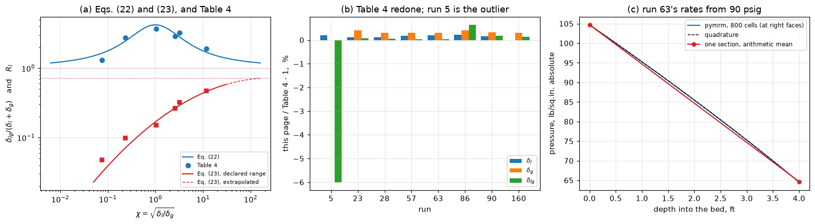
Validation
What is being validated, ranked
- The worked example. Table 3 to Table 4 is the authors’ own arithmetic, printed in full. Reproducing it tests the transcription, the equations, the constants, the unit conversions and the manometer correction all at once, against numbers nobody on this page chose. This is where the page’s weight sits.
- Two asymptotic checks the paper states for its own data. Run 160 is gas alone (\(\chi \to 0\)) and run 5 liquid alone (\(\chi \to \infty\)), and the paper says the two-phase parameter approaches unity at both ends. These are asymptotic statements about the Figure 7 cloud, not per-row requirements, and step 3 weighs both rows against the scatter the same paper prints for that cloud.
- A stated result in the text: the average-pressure claim of book p. 236, checked algebraically for one phase and numerically for two, with three independent routes to the column and a discrete balance.
- Nothing from a figure. The correlation curves plotted above are the printed equations.
And what is NOT validation. The comparison of Eqs. (22)/(23) with Table 4 is a goodness of fit to data inside the fit. It is on the page because the size of the residuals is informative, and it is printed beside two nulls so that it cannot be read as more.
Every number, registered
Each number the page states is registered below with how it is checked (gallery_utils.Claims): a value held to a tolerance of its committed result, a bound checked whenever the page runs (identities, solver tolerances, convergence orders), or an exact count with its margin to the threshold that decided it.
def run_blocks(cfg, which=("repro", "recon", "run5", "self", "corr", "shape", "col",
                              "outlet", "spread")):
    """Every claimed number of the named blocks, recomputed under ``cfg``."""
    blocks = {"repro": block_repro, "recon": block_recon, "run5": block_run5,
              "self": block_selfcheck, "corr": block_corr, "shape": block_shape,
              "col": block_col, "outlet": block_outlet, "spread": block_spread}
    out = {}
    for k in which:
        out.update({a: b for a, b in blocks[k](cfg).items() if not a.startswith("_")})
    return out


ALL = run_blocks(BASE)
TOL = "newton tol 1e-10 psi on pressures near 100 psia"
EXACT_ID = dict(basis="identity")
for name, x in ALL.items():
    if name in ("delta_l_two_unit_systems_max_rel_diff",):
        claims.bound(name, x, max=1e-13, **EXACT_ID,
                     note="the same Eq. (17) in two unit systems sharing every Cfg input")
    elif name == "run5_ergun_residual_is_parameter_gap":
        claims.bound(name, x, max=1e-12, **EXACT_ID, note="delta_g = 0 on run 5")
    elif name == "gas_horizontal_arith_mean_max_rel_error":
        claims.bound(name, x, max=1e-11, **EXACT_ID,
                     note="delta_g = K/P makes P^2 linear in z; recipe and quadrature at round-off")
    elif name == "eq22_argmax_chi":
        claims.bound(name, x, min=1 - 1e-8, max=1 + 1e-8, **EXACT_ID,
                     note="Eq. (22) is even in log10 chi; brentq xtol 1e-13")
    elif name == "eq23_argmax_root_vs_analytic_rel":
        claims.bound(name, x, max=1e-8, basis="tolerance",
                     note="root of a centred difference with relative step 1e-6")
    elif name == "fv_observed_order":
        claims.bound(name, x, min=0.95, max=1.05, basis="theory", note="first-order upwind")
    elif name == "sectioning_observed_order":
        claims.bound(name, x, min=1.95, max=2.05, basis="theory",
                     note="the arithmetic mean of the terminals is the midpoint rule")
    elif name == "fv_richardson_remainder_order":
        claims.bound(name, x, min=1.9, max=2.1, basis="theory",
                     note="the Richardson pair of a first-order scheme leaves an O(h^2) remainder")
    elif name == "fv_richardson_remainder_finest_over_noise":
        claims.bound(name, x, min=1e3, basis="theory",
                     note=f"remainder of the (1600, 3200) pair over the {TOL}")
    elif name == "zg_first_cell_face_over_centre_distance":
        claims.bound(name, x, max=0.05, basis="theory",
                     note="backward Euler: O(h^2) from the right face, O(h) from the centre")
    elif name == "fv_finest_err_over_noise":
        claims.bound(name, x, min=1e3, basis="theory", note=f"error at 1600 cells over the {TOL}")
    elif name == "sectioning_finest_err_over_noise":
        claims.bound(name, x, min=1e3, basis="theory",
                     note="error at 64 sections over the fixed-point tolerance 1e-14")
    elif name in ("fv_outflow_vs_hand_march_rel", "fv_balance_gap", "zg_outlet_flux_vs_face_value",
                  "zg_face_correction_over_ninth"):
        claims.bound(name, x, max=1e-10, **EXACT_ID, note=f"round-off; {TOL}")
    elif name == "zg_outlet_row_last_weight":
        claims.bound(name, x, min=1.125 - 1e-12, max=1.125 + 1e-12, **EXACT_ID,
                     note="zero-gradient outlet folded into the flux: 9/8")
    elif name == "zg_outlet_row_prev_weight":
        claims.bound(name, x, min=-0.125 - 1e-12, max=-0.125 + 1e-12, **EXACT_ID,
                     note="zero-gradient outlet folded into the flux: -1/8")
    elif name == "zg_last_step_over_h":
        claims.bound(name, x, min=8 / 9 - 1e-9, max=8 / 9 + 1e-9, **EXACT_ID,
                     note="the last cell's balance with the folded outlet")
    elif name in ("eq23_rows_outside_20pct", "eq23_fig7_rows_outside_20pct"):
        dev = C["_rdev"] if name == "eq23_rows_outside_20pct" else C["_f7dev"]
        claims.count(name, np.abs(dev), 20.0, min_margin=0.02)
    elif name == "two_phase_recipe_1pct_runs_inside_experimental_column":
        claims.count(name, list(SPR["_lens"].values()), KV["experimental_column_length"],
                     above=False, min_margin=0.02)
    elif name == "two_phase_recipe_1pct_runs_inside_commercial_reactor":
        claims.count(name, list(SPR["_lens"].values()), KV["commercial_reactor_length"],
                     above=False, min_margin=0.02)
    else:
        # deterministic arithmetic, root-finds and grid errors: spread below 1e-12
        claims.value(name, x, rtol=1e-3)
print(f"{len(claims.metrics)} claims registered")
103 claims registeredThe break table
Every row below injects one defect, a transcribed constant read wrongly, a table cell read wrongly, a modelling choice or a numerical setting, re-runs the same block functions that produced the registered numbers, and hands each recomputed number to claims.breaks, which records whether that claim’s own check (its tolerance or its bound) catches it. Every claim must be caught by at least one row; the last cell raises otherwise. Rows that read a table cell wrongly are what reach the statistics of the printed tables (the nulls, the self-consistency checks, the run-5 arithmetic), which no constant touches.
def cell(table, run, column, value):
    """A copy of ``table`` with one cell read differently."""
    t = table.copy()
    t.loc[t.run == run, column] = value
    return t


ROWS = [
    ("alpha transcribed as Ergun's 150 (the paper prints 266)",
     dict(alpha=KV["cylinder_alpha"]), ("repro", "run5", "col")),
    ("beta transcribed as 1.75 (the paper prints 2.33)",
     dict(beta=KV["cylinder_beta"]), ("repro", "run5", "col")),
    ("specific surface at 147.5, the bottom of what '148' rounds from",
     dict(s_surf=147.5), ("repro", "recon", "run5", "col")),
    ("specific surface at 148.5, the top of the same interval",
     dict(s_surf=148.5), ("repro", "recon", "run5", "col")),
    ("the manometer correction of book p. 236 left out",
     dict(manometer=False), ("repro", "run5")),
    ("rho_m taken as the liquid density instead of Eq. (21)'s mixture",
     dict(rho_m_mode="liquid"), ("repro", "run5")),
    ("air viscosity fixed at Table 2's 0.0192 cP instead of the recovered line",
     dict(mu_air_mode="table2"), ("repro", "col", "outlet", "spread")),
    ("Table 2's air viscosity 0.0192 read as 0.0129",
     dict(mu_air_table2=0.0129), ("repro", "recon")),
    ("D_p taken as the nominal 3/8 in. instead of Eq. (19)'s 6(1-eps)/S",
     dict(dp_override=0.375 / 12.0), ("repro", "recon", "run5", "col")),
    ("g_c taken at the exact 32.174 instead of the printed 32.17",
     dict(gc=32.174049), ("repro", "run5", "col")),
    ("standard atmosphere taken as 14.7 instead of 14.696",
     dict(p_atm=14.7), ("repro", "run5", "col")),
    ("Table 2's air density read as at 80 F instead of at 32 F",
     dict(t_air_ref=80.0), ("repro", "run5", "col")),
    ("1 centipoise rounded to 6.72e-4 lb/(ft.sec)",
     dict(cp=6.72e-4 * 60.0), ("repro", "recon")),
    ("the ft-lb-second route given its own rounded centipoise",
     dict(primitive_cp=6.72e-4 * 60.0), ("repro",)),
    ("porosity taken as the 3/8-in. sphere value 0.362",
     dict(eps=KV["sphere_bed_porosity"]), ("repro", "recon", "run5", "spread")),
    ("Eq. (22) read with natural logs instead of log10",
     dict(eq22_ln=True), ("corr", "shape", "col")),
    ("Eq. (22)'s two constants swapped",
     dict(eq22_a=KV["eq22_offset"], eq22_b=KV["eq22_numerator"]), ("corr", "shape")),
    ("Eq. (23)'s linear coefficient read as 0.252, a transposition of 0.525",
     dict(eq23_c=(KV["eq23_c0"], 0.252, KV["eq23_c2"])), ("corr", "shape", "col")),
    ("Eq. (23) taken with the constant term Figure 7 prints, -0.744",
     dict(eq23_c=(KV["eq23_c0_figure7"], KV["eq23_c1"], KV["eq23_c2"])),
     ("corr", "shape", "col", "spread")),
    ("chi defined as sqrt(delta_g/delta_l), the reciprocal of the printed one",
     dict(chi_inverted=True), ("corr", "col")),
    ("the gravity term of Eq. (5) dropped from the column",
     dict(gravity=False), ("col",)),
    ("the two-phase correlation switched off: delta_lg = delta_l + delta_g",
     dict(two_phase=False), ("col",)),
    ("the section evaluated at its inlet pressure, not the mean of its terminals",
     dict(mean_rule="inlet"), ("col", "spread")),
    ("the geometric mean of the terminals instead of the arithmetic one",
     dict(mean_rule="geometric"), ("col",)),
    ("extrema and thresholds sampled on a grid instead of root-found",
     dict(rootfind=False), ("shape", "col")),
    ("the root-finder's tolerance loosened to 1e-4",
     dict(root_xtol=1e-4), ("shape",)),
    ("the grid pair 1200 and 1600 cells read as a doubling",
     dict(n_fv=(1200, 1600)), ("col",)),
    ("the column solved on 50 and 100 cells instead of 800 and 1600",
     dict(n_fv=(50, 100)), ("col", "outlet")),
    ("Newton tolerance loosened to 1e-3",
     dict(newton_tol=1e-3), ("col",)),
    ("the recipe's fixed point stopped at 1e-6",
     dict(recipe_tol=1e-6), ("col",)),
    ("zero-gradient outlet, read from the last cell (pitfall P8)",
     dict(outlet="zero_gradient", read="cell"), ("col", "outlet")),
    ("zero-gradient outlet, read on the face",
     dict(outlet="zero_gradient"), ("col", "outlet")),
    ("the demonstration column built on the mildest two-phase row (run 86)",
     dict(demo_run=86), ("col", "outlet")),
    ("Table 4 air Reynolds of run 63 read as 4515 (printed 4155)",
     dict(t4=cell(T4, 63, "reynolds_air", 4515.0)), ("recon",)),
    ("Table 4 two-phase parameter of run 28 read as 3.865 (printed 3.685)",
     dict(t4=cell(T4, 28, "two_phase_parameter", 3.865)), ("corr", "self")),
    ("Table 3 liquid saturation of run 57 read as 41.0 (printed 47.0)",
     dict(t3=cell(T3, 57, "liquid_saturation_pct", 41.0)), ("corr",)),
    ("Table 4 delta_lg of run 5 read as 2.496 (printed 2.469)",
     dict(t4=cell(T4, 5, "delta_lg_psi_per_ft", 2.496)), ("run5",)),
    ("Table 4 delta_g of run 5 read as 0.0226 (printed 0)",
     dict(t4=cell(T4, 5, "delta_g_psi_per_ft", 0.0226)), ("run5",)),
    ("Table 4 delta_g of run 160 read as 1.983 (printed 1.938)",
     dict(t4=cell(T4, 160, "delta_g_psi_per_ft", 1.983)), ("run5",)),
    ("Table 4 two-phase parameter of run 160 read as 1.090 (printed 1.009)",
     dict(t4=cell(T4, 160, "two_phase_parameter", 1.090)), ("run5",)),
    ("Table 4 chi of run 23 read as 3.502 (printed 3.205)",
     dict(t4=cell(T4, 23, "chi", 3.502)), ("self",)),
    ("Table 3 liquid rate of run 86 read as 79.93 (printed 97.93)",
     dict(t3=cell(T3, 86, "liquid_rate_lb_sqft_min", 79.93)), ("repro",)),
]

BREAK = []
for label, changes, which in ROWS:
    got = run_blocks(make(**changes), which)
    caught = [n for n, v in got.items() if n in claims.metrics and claims.breaks(label, n, v)]
    BREAK.append((label, len(got), caught))

# the zero-gradient comparison's own claims: built with the outflow marker, the
# folded row, the shortened step and the face correction all disappear
_zg = ColumnFV(col, PIN, L4, 100, outlet="outflow")
_Pz = _zg.solve()
_row = np.asarray(_zg.conv.todense())[-1]
_label = "the zero-gradient comparison built with the outflow marker instead"
_caught = [n for n, v in {
    "zg_outlet_row_last_weight": float(_row[-1]),
    "zg_outlet_row_prev_weight": float(_row[-2]),
    "zg_last_step_over_h": float((_Pz[-1] - _Pz[-2]) / (L4 / 100) / col.dPdz(_Pz[-1])),
}.items() if claims.breaks(_label, n, v)]
BREAK.append((_label, 3, _caught))
# the same last-cell balance with the outflow marker: it closes, as the face read does
_rows2 = {}
for _n, _name in ((100, "zg_lastcell_balance_gap_n100"), (1600, "zg_lastcell_balance_gap_nfine")):
    _o = ColumnFV(col, PIN, L4, _n, outlet="outflow")
    _rows2[_name] = float(abs(_o.balance_gap(_o.solve(), "cell")))
_l2 = "the last-cell balance taken with the outflow marker instead of the zero-gradient outlet"
BREAK.append((_l2, 2, [n for n, v in _rows2.items() if claims.breaks(_l2, n, v)]))
# the first cell read as a centre value: the distance ratio inverts
_o = ColumnFV(col, PIN, L4, 100)
_p1 = float(_o.solve()[0])
_l3 = "cell values located at cell centres instead of right faces"
_inv = abs(_p1 - quad_outlet(col, PIN, float(_o.x_c[0]))) / abs(_p1 - quad_outlet(col, PIN, float(_o.x_f[1])))
BREAK.append((_l3, 1, ["zg_first_cell_face_over_centre_distance"]
              if claims.breaks(_l3, "zg_first_cell_face_over_centre_distance", _inv) else []))
# the face value against the flux the operator transports, with the last cell read instead
_P = OUT["_P"]
if claims.breaks("zero-gradient flux compared with the last cell (pitfall P8)",
                 "zg_outlet_flux_vs_face_value", float(abs(OUT["_flux_out"] / _P[-1] - 1.0))):
    BREAK.append(("zero-gradient flux compared with the last cell (pitfall P8)", 1,
                  ["zg_outlet_flux_vs_face_value"]))
# the face correction measured against h S/8 instead of h S/9
if claims.breaks("the face correction taken as h S/8", "zg_face_correction_over_ninth",
                 float(abs((OUT["_cbv"] - _P[-1]) / (OUT["_h"] * OUT["_S_N"] / 8.0) - 1.0))):
    BREAK.append(("the face correction taken as h S/8", 1, ["zg_face_correction_over_ninth"]))

caught_by = {}
for label, n, caught in BREAK:
    for c in caught:
        caught_by.setdefault(c, []).append(label)
lines = [f"{len(BREAK)} rows; per row: claims recomputed, claims caught"]
lines += [f"  {n:3d} {len(c):3d}  {label}" for label, n, c in BREAK]
miss = sorted(set(claims.metrics) - set(caught_by))
lines += [f"\n{len(caught_by)} of {len(claims.metrics)} claims caught by at least one row;"
          f" not caught: {miss if miss else 'none'}"]
print("\n".join(lines))
47 rows; per row: claims recomputed, claims caught
42 15 alpha transcribed as Ergun's 150 (the paper prints 266)
42 16 beta transcribed as 1.75 (the paper prints 2.33)
49 21 specific surface at 147.5, the bottom of what '148' rounds from
49 21 specific surface at 148.5, the top of the same interval
24 8 the manometer correction of book p. 236 left out
24 4 rho_m taken as the liquid density instead of Eq. (21)'s mixture
51 3 air viscosity fixed at Table 2's 0.0192 cP instead of the recovered line
19 3 Table 2's air viscosity 0.0192 read as 0.0129
49 25 D_p taken as the nominal 3/8 in. instead of Eq. (19)'s 6(1-eps)/S
42 3 g_c taken at the exact 32.174 instead of the printed 32.17
42 1 standard atmosphere taken as 14.7 instead of 14.696
42 14 Table 2's air density read as at 80 F instead of at 32 F
19 7 1 centipoise rounded to 6.72e-4 lb/(ft.sec)
12 1 the ft-lb-second route given its own rounded centipoise
35 9 porosity taken as the 3/8-in. sphere value 0.362
49 17 Eq. (22) read with natural logs instead of log10
31 8 Eq. (22)'s two constants swapped
49 21 Eq. (23)'s linear coefficient read as 0.252, a transposition of 0.525
53 15 Eq. (23) taken with the constant term Figure 7 prints, -0.744
38 14 chi defined as sqrt(delta_g/delta_l), the reciprocal of the printed one
18 8 the gravity term of Eq. (5) dropped from the column
18 9 the two-phase correlation switched off: delta_lg = delta_l + delta_g
22 10 the section evaluated at its inlet pressure, not the mean of its terminals
18 5 the geometric mean of the terminals instead of the arithmetic one
29 3 extrema and thresholds sampled on a grid instead of root-found
11 2 the root-finder's tolerance loosened to 1e-4
18 5 the grid pair 1200 and 1600 cells read as a doubling
35 11 the column solved on 50 and 100 cells instead of 800 and 1600
18 2 Newton tolerance loosened to 1e-3
18 3 the recipe's fixed point stopped at 1e-6
35 10 zero-gradient outlet, read from the last cell (pitfall P8)
35 6 zero-gradient outlet, read on the face
35 19 the demonstration column built on the mildest two-phase row (run 86)
7 4 Table 4 air Reynolds of run 63 read as 4515 (printed 4155)
22 11 Table 4 two-phase parameter of run 28 read as 3.865 (printed 3.685)
20 5 Table 3 liquid saturation of run 57 read as 41.0 (printed 47.0)
12 4 Table 4 delta_lg of run 5 read as 2.496 (printed 2.469)
12 4 Table 4 delta_g of run 5 read as 0.0226 (printed 0)
12 2 Table 4 delta_g of run 160 read as 1.983 (printed 1.938)
12 1 Table 4 two-phase parameter of run 160 read as 1.090 (printed 1.009)
2 1 Table 4 chi of run 23 read as 3.502 (printed 3.205)
12 6 Table 3 liquid rate of run 86 read as 79.93 (printed 97.93)
3 3 the zero-gradient comparison built with the outflow marker instead
2 2 the last-cell balance taken with the outflow marker instead of the zero-gradient outlet
1 1 cell values located at cell centres instead of right faces
1 1 zero-gradient flux compared with the last cell (pitfall P8)
1 1 the face correction taken as h S/8
103 of 103 claims caught by at least one row; not caught: nonePrinted features, reported and not repaired
1. Table 3 and Table 4 disagree about run 5. Table 3’s run-5 pressure drop is 2.321, Table 4’s run-5 \(\delta_{lg}\) is 2.469, and for a run with no gas Eq. (20) makes those the same number. Established from the paper’s own arithmetic above; not repaired, and this page does not say which cell is wrong.
2. Eq. (23) is printed twice on book p. 237 with two different constant terms. The typeset equation is
log_10 R_l = - 0.774 + 0.525 (log_10 chi) - 0.109 (log_10 chi)^2
and the annotation inside Figure 7, on the facing column of the same page, is
log_10 R_l = -0.744 + 0.525 log_10 X - 0.109 (log_10 X)^2
Every other coefficient agrees, and so does the whole of Eq. (22), which Figure 7 also prints in full. Both were read on 300 ppi crops enlarged to digit scale; the difference is a transposition. Figures 3, 5 and 6 carry the same curves but print only the labels “EQUATION (22)” and “EQUATION (23)” beside them, not the coefficients (each was cropped and read), so Figure 7 is the only second printing of either equation in the paper. Neither reading is adopted, and the paper’s own printed data cannot settle it (Results).
3. The notation’s units make Eq. (17) inconsistent with the printed \(g_c\). Verbatim: mu = viscosity, (lb. mass/ft.-min.) and g_c = conversion factor, 32.17 pdl./lb.-mass in English units. With \(\mu\) on those units Eq. (17) reproduces Table 4 only if the conversion factor carries \(\mathrm{min}^{-2}\), i.e. \(32.17 \times 3600\); the factor the table requires is measured above at 3593.8. Separately, “pdl./lb.-mass” is an acceleration, \(g_c\) being poundals per pound-force, but that is a reading of the words rather than of the arithmetic. Neither is repaired.
4. Not a defect. Eq. (23) cannot return a full column for any \(\chi\), and its maximum sits more than eight times beyond the upper limit it is declared for. The paper says on book p. 238 that Eq. (23) “is a power series fit which is only good within the limits given”, and it attributes the \(R_l \to 1\) and \(R_l \to 0\) consistency checks to “the data of Figure 7” rather than to the equation. The numbers on this page quantify a caveat the authors print.
Where the search for these went. All nine pages were rendered at their native 300 ppi and read; the numerals of Tables 2, 3, 4 and 5, of Eqs. (17) to (23), and of every equation annotated inside Figures 3, 5, 6 and 7 were re-read on enlarged crops at digit scale. The claim that no footnote attaches to Table 3 or Table 4 was checked by cropping the strip beneath each table. The claim that the tables are discussed nowhere else was checked by reading both sections that name them in full, plus the “PRESENTATION OF CORRELATED DATA” section that follows. Reference 4, the thesis, is not on disk, so nothing here rules out that it addresses run 5.
What pymrm adds
Not the correlation, and not the worked example. Eqs. (17)-(23) are arithmetic. The reproduction of Table 4 above uses NumPy and nothing else.
What pymrm buys is the question the 1961 procedure could only answer by judgement. The paper’s design calculation is a march with an assumed average pressure per section, iterated to consistency, and its own step 1 tells the reader to split the bed when it is long or the loss is large, without saying how long or how many sections. Written as a differential equation and solved on a grid, the same physics answers both questions:
- the one-section recipe is exact for a single phase in horizontal flow, proved algebraically above and confirmed at round-off, so the sectioning advice is not about compressibility as such;
- with the two-phase correlation in the loop it reaches 1 % at a bed length root-found on the page: inside the paper’s own column for the largest-friction-loss row of Table 3, and far outside the 40-ft commercial reactor for the mildest;
- sectioning converges at second order, so the number of sections needed for a target accuracy follows from one number instead of from judgement.
The assembly is small: construct_convflux_upwind and construct_div at \(v = 1\), an inlet dictionary and the {"outflow": True} outlet, NumJac((n, 1)) for a pointwise source, newton, and compute_boundary_values for the outlet. What it is worth is not speed (a quadrature does this problem too, and is used here as the independent route) but that the same operators carry over the moment anything else is added to the column: a reaction, a species balance, a heat balance, or a second spatial dimension.
An honest limit. Nothing in this section is validated against a measurement. The paper reports no axial pressure profile, only a per-foot gradient from a middle section. What is validated is the arithmetic: three independent routes to the same profile, a discrete balance, and an identity that can be proved.
Reuse
| Change | Where |
|---|---|
| A different packing | alpha, beta, eps, s_surf of Larkins (Larkins.from_constants(KV, alpha=..., ...)); book p. 236 prints (118.2, 1.0) for 3/8-in. spheres and Ergun’s own (150, 1.75) for cylinders, neither of which any printed data on this page exercises |
| A different gas-liquid system | rho_w, rho_air_ref, t_air_ref and the air viscosity (mu_air_mode="table2" with mu_air_table2, or your own mu_air_line); Table 2 carries eleven fluids |
| Horizontal flow | Larkins.from_constants(KV, gravity=False) drops the static head |
| Upflow | the static head opposes the flow: change the sign of the \(\rho_m\) term in Column.dPdz (with \(z\) along the flow) |
| A reaction in the bed | add species fields to ColumnFV: the shape becomes (n, 1 + n_c) and NumJac((n, 1 + n_c)) couples the last axis in full. The v = 1 of the pressure equation is only a device for marching it; species are convected with their own phase velocities, so they need their own convection operators |
| Heat as well | a temperature field in the same state, with its own bc dictionaries; the S3 pattern is unchanged |
| A hold-up closure instead of Eq. (23) | replace Larkins.f23; G1.7 (Wammes) is the high-pressure alternative and G1.8 the partial-wetting one |
The outlet of a convection-only column takes {"outflow": True}; a zero-gradient dictionary there imposes a condition the problem does not have (measured above).
Related pages: G1.7 Wammes-Westerterp high-pressure trickle-bed hydrodynamics, the same coupled hold-up/pressure-gradient structure at 7.5 MPa · G1.8 trickle-bed partial wetting · A1.1 Ergun, which is Eq. (17) with \(\alpha = 150\), \(\beta = 1.75\) · F2.3 slurry bubble columns · F1.4 Krishna-Ellenberger hold-up.
Do not reuse the run-5 row as data. It is on this page as an unresolved discrepancy, not as a measurement, and the CSV’s sidecar says so.
References
The source, read. Larkins, R. P., White, R. R. and Jeffrey, D. W. (1961). Two-Phase Concurrent Flow in Packed Beds. AIChE Journal 7(2), 231-239. doi:10.1002/aic.690070213. Identity confirmed on the file’s own title page: the title, the by-line “R. P. LARKINS and R. R. WHITE / University of Michigan, Ann Arbor, Michigan” and “D. W. JEFFREY / Humble Oil and Refining Company, Baytown, Texas”, the abstract, and the present-address footnote. PDF page 1 opens with the NOMENCLATURE and “Manuscript received April 18, 1960” of the PRECEDING article, a film-theory/penetration-theory paper; Larkins et al. begin below the rule on the same page. Book page = PDF page + 230.
Cited by the paper, not on disk, not read. Larkins, R. P. (1959). PhD thesis, University of Michigan, Ann Arbor: the paper’s reference 4, “the complete tabulation of properties, data and results”, offered on microfilm. It is also the support the paper gives for the average-pressure claim this page tests, so what is shown there, and under what assumptions, is unknown here.
Named in the paper, not evaluated here. Ergun, S. (1952), Chem. Eng. Progr. 48, 89 (reference 3, the origin of Eq. (17)’s form and of the (150, 1.75) pair). Brownell, L. E. and Katz, D. L. (1947), Chem. Eng. Progr. 43, 537 (reference 2). Lockhart, R. W. and Martinelli, R. C. (1949), Chem. Eng. Progr. 45, 39 (reference 6, whose \(X\) this paper’s \(\chi\) mirrors). Piret, E. L., Mann, C. A. and Wall, T. Jr. (1940), Ind. Eng. Chem. 32, 861 (reference 9). None of the four is on disk; each is cited, not used.
# prose numbers: the Markdown cells of this notebook (README.md tags its own)
for lit, name in [
    # Parameters and assumptions
    ("0.026", "mu_air_linear_fit_max_resid_pct"),
    # Step 2 heading
    ("0.15", "reynolds_systematic_offset_pct"),
    # Step 3 and run 5
    ("-5.99", "run5_delta_lg_rel_error_pct"), ("0.639", "delta_lg_max_rel_error_pct"),
    ("+22.29", "run160_manometer_correction_worth_pct"),
    ("0.9408", "run5_two_phase_parameter_from_table3"),
    ("-5.92", "run5_parameter_gap_from_unity_pct"),
    ("+0.90", "run160_parameter_off_unity_pct"),
    ("0.93", "run160_vs_ergun_pct"), ("0.081", "run5_vs_ergun_pct"),
    ("11.5", "run5_closer_factor"),
    # Results: correlations
    ("25.53", "eq22_max_abs_dev_pct"), ("12.81", "eq22_rms_dev_pct"),
    ("4.05", "eq22_gain_over_bestconst"), ("2.48", "eq22_free_rows_gain_over_bestconst"),
    ("14.79", "eq22_free_rows_rms_dev_pct"), ("63", "eq22_gain_flatters_pct"),
    ("33.90", "eq23_max_abs_dev_pct"), ("19.55", "eq23_rms_dev_pct"),
    ("117.9", "eq23_null_bestconst_rms_dev_pct"),
    ("7.15", "eq23_fig7_constant_worth_pct"), ("18.33", "eq23_fig7_rms_dev_pct"),
    ("256.010", "eq23_argmax_chi"), ("0.7214", "eq23_ceiling_liquid_saturation"),
    ("-0.0618", "eq23_discriminant_at_saturation_unity"),
    ("0.7730", "eq23_fig7_ceiling_liquid_saturation"), ("-0.0488", "eq23_fig7_discriminant"),
    ("2.283 %", "eq23_at_chi_lower_limit"), ("58.03 %", "eq23_at_chi_upper_limit"),
    # Results: column
    ("below 1e-11", "gas_horizontal_arith_mean_max_rel_error"),
    ("1.12e-05", "gas_horizontal_geom_mean_max_rel_error"),
    ("1.72e-07", "gas_downflow_arith_mean_rel_error_2ft"),
    ("129", "gas_friction_over_static_head_at_inlet"),
    ("0.332 %", "two_phase_recipe_rel_error_4ft"),
    ("5.6012", "two_phase_recipe_1pct_length_ft"),
    ("5.6012", "two_phase_recipe_1pct_length_min_ft"),
    ("466.9537", "two_phase_recipe_1pct_length_max_ft"),
    ("1", "two_phase_recipe_1pct_runs_inside_experimental_column"),
    ("4", "two_phase_recipe_1pct_runs_inside_commercial_reactor"),
    ("8.0627", "choking_length_ft"), ("1.9999", "sectioning_observed_order"),
    ("3.84", "cbv_over_upwind_face_outlet_error_ratio"),
    # Printed features
    ("3593.8", "gc_minute_conversion_recovered"),
    # the outlet condition
    ("1.2e-3", "zg_lastcell_balance_gap_n100"), ("7.7e-5", "zg_lastcell_balance_gap_nfine"),
    ("+9.85e-06", "zg_lastcell_error_signed_nfine"), ("-3.78e-05", "fv_error_signed_n_fine"),
    ("2.00", "fv_richardson_remainder_order"),
]:
    claims.says(lit, name)
# meta.yaml (validation, adds, agreement) and the models.yaml entry
for lit, name in [
    ("0.174", "re_liquid_max_rel_error_pct"), ("0.147", "re_liquid_rms_rel_error_pct"),
    ("0.218", "delta_l_max_rel_error_pct"), ("0.176", "delta_l_rms_rel_error_pct"),
    ("0.416", "delta_g_max_rel_error_pct"), ("0.639", "delta_lg_max_rel_error_pct"),
    ("0.260", "delta_lg_rms_rel_error_pct"), ("-5.99", "run5_delta_lg_rel_error_pct"),
    ("0.9408", "run5_two_phase_parameter_from_table3"),
    ("-5.92", "run5_parameter_gap_from_unity_pct"), ("+0.90", "run160_parameter_off_unity_pct"),
    ("0.081", "run5_vs_ergun_pct"), ("11.5", "run5_closer_factor"), ("0.93", "run160_vs_ergun_pct"),
    ("+22.29", "run160_manometer_correction_worth_pct"),
    ("0.0259", "mu_air_linear_fit_max_resid_pct"), ("0.819", "mu_air_at_80F_vs_table2_pct"),
    ("0.672", "mu_air_at_80F_offset_corrected_vs_table2_pct"),
    ("28", "mass_rate_range_fold"), ("+0.1454", "reynolds_systematic_offset_pct"),
    ("0.0515", "reynolds_offset_spread_pct"), ("148.22", "reynolds_offset_implied_specific_surface"),
    ("below 1e-13", "delta_l_two_unit_systems_max_rel_diff"),
    ("3593.8", "gc_minute_conversion_recovered"),
    ("below 1e-11", "gas_horizontal_arith_mean_max_rel_error"),
    ("1.12e-05", "gas_horizontal_geom_mean_max_rel_error"),
    ("0.332 %", "two_phase_recipe_rel_error_4ft"), ("5.6012", "two_phase_recipe_1pct_length_ft"),
    ("5.6012", "two_phase_recipe_1pct_length_min_ft"),
    ("466.9537", "two_phase_recipe_1pct_length_max_ft"),
    ("1", "two_phase_recipe_1pct_runs_inside_experimental_column"),
    ("4", "two_phase_recipe_1pct_runs_inside_commercial_reactor"),
    ("1.9999", "sectioning_observed_order"), ("1.0003", "fv_observed_order"),
    ("1.47e-08", "fv_extrapolated_vs_quadrature_rel"), ("5.35", "fv_extrap_orders_below_recipe"),
    ("below 1e-10", "fv_outflow_vs_hand_march_rel"), ("below 1e-10", "fv_balance_gap"),
    ("1.2e-3", "zg_lastcell_balance_gap_n100"), ("2.00", "fv_richardson_remainder_order"),
    ("3.84", "cbv_over_upwind_face_outlet_error_ratio"),
    ("7.15", "eq23_fig7_constant_worth_pct"), ("18.33", "eq23_fig7_rms_dev_pct"),
    ("19.55", "eq23_rms_dev_pct"), ("3", "eq23_fig7_rows_outside_20pct"),
    ("2", "eq23_rows_outside_20pct"),
    ("0.7730", "eq23_fig7_ceiling_liquid_saturation"), ("0.7214", "eq23_ceiling_liquid_saturation"),
    ("256.010", "eq23_argmax_chi"), ("-0.0618", "eq23_discriminant_at_saturation_unity"),
    ("25.53", "eq22_max_abs_dev_pct"), ("12.81", "eq22_rms_dev_pct"), ("33.90", "eq23_max_abs_dev_pct"),
    ("4.05", "eq22_gain_over_bestconst"), ("2.48", "eq22_free_rows_gain_over_bestconst"),
    ("14.79", "eq22_free_rows_rms_dev_pct"),
]:
    claims.says(lit, name)
# Claims: prints every registered number, writes agreement.json for CI, and
# raises when a claim fails its own check or has no break row.
claims.report(); # the semicolon keeps the notebook from echoing the payloadClaims for G1.1:
re_liquid_max_rel_error_pct = 0.17406 value rtol 0.001
re_liquid_rms_rel_error_pct = 0.14652 value rtol 0.001
re_air_table2_viscosity_max_rel_error_pct = 2.2116 value rtol 0.001
delta_l_max_rel_error_pct = 0.21769 value rtol 0.001
delta_l_rms_rel_error_pct = 0.17568 value rtol 0.001
delta_g_max_rel_error_pct = 0.41615 value rtol 0.001
delta_lg_max_rel_error_pct = 0.63899 value rtol 0.001
delta_lg_rms_rel_error_pct = 0.26001 value rtol 0.001
delta_l_two_unit_systems_max_rel_diff = (here 5.6e-16) bound bound <= 1e-13 [identity]
gc_minute_conversion_recovered = 3593.8 value rtol 0.001
mass_rate_range_fold = 27.887 value rtol 0.001
dp_nominal_over_effective_pct = 60.59 value rtol 0.001
reynolds_systematic_offset_pct = 0.14538 value rtol 0.001
reynolds_offset_spread_pct = 0.051539 value rtol 0.001
reynolds_offset_implied_specific_surface = 148.22 value rtol 0.001
mu_air_linear_fit_max_resid_pct = 0.025861 value rtol 0.001
mu_air_slope_cP_per_degF = 2.7649e-05 value rtol 0.001
mu_air_at_80F_vs_table2_pct = 0.81858 value rtol 0.001
mu_air_at_80F_offset_corrected_vs_table2_pct = 0.67222 value rtol 0.001
run5_delta_lg_rel_error_pct = -5.9943 value rtol 0.001
run5_dpdl_implied_by_table4_psi_per_ft = 2.469 value rtol 0.001
run5_two_phase_parameter_from_table3 = 0.94082 value rtol 0.001
run5_parameter_gap_vs_printed = 0.060181 value rtol 0.001
run5_parameter_gap_from_unity_pct = -5.9181 value rtol 0.001
run160_delta_lg_rel_error_pct = 0.13392 value rtol 0.001
run160_manometer_correction_worth_pct = 22.288 value rtol 0.001
run5_vs_ergun_pct = 0.08107 value rtol 0.001
run160_vs_ergun_pct = 0.92879 value rtol 0.001
run5_closer_factor = 11.457 value rtol 0.001
run160_parameter_off_unity_pct = 0.9 value rtol 0.001
run5_ergun_residual_is_parameter_gap = (here 0.0e+00) bound bound <= 1e-12 [identity]
t4_chi_selfcheck_max_pct = 0.053021 value rtol 0.001
t4_parameter_selfcheck_max_pct = 0.065134 value rtol 0.001
eq22_max_abs_dev_pct = 25.53 value rtol 0.001
eq22_rms_dev_pct = 12.812 value rtol 0.001
eq22_rms_log_dev = 0.053082 value rtol 0.001
eq22_null_unity_rms_log_dev = 0.36662 value rtol 0.001
eq22_null_bestconst_rms_log_dev = 0.21515 value rtol 0.001
eq22_gain_over_bestconst = 4.0531 value rtol 0.001
eq22_free_rows_rms_dev_pct = 14.789 value rtol 0.001
eq22_free_rows_rms_log_dev = 0.061273 value rtol 0.001
eq22_free_rows_null_bestconst_rms_log_dev = 0.15205 value rtol 0.001
eq22_free_rows_gain_over_bestconst = 2.4815 value rtol 0.001
eq23_max_abs_dev_pct = 33.898 value rtol 0.001
eq23_rms_dev_pct = 19.551 value rtol 0.001
eq23_null_bestconst_rms_dev_pct = 117.94 value rtol 0.001
eq23_rows_outside_20pct = 2 exact exact, margin 0.275
eq23_fig7_rms_dev_pct = 18.327 value rtol 0.001
eq23_fig7_max_abs_dev_pct = 29.17 value rtol 0.001
eq23_fig7_rows_outside_20pct = 3 exact exact, margin 0.135
eq23_text_minus_fig7_rms_dev_pct = 1.2232 value rtol 0.001
eq22_gain_flatters_pct = 63.332 value rtol 0.001
eq23_gain_over_bestconst = 6.0325 value rtol 0.001
eq22_argmax_chi = (here 1.0e+00) bound bound [1, 1] [identity]
eq22_max_parameter = 4.2133 value rtol 0.001
eq23_argmax_chi = 256.01 value rtol 0.001
eq23_argmax_root_vs_analytic_rel = (here 2.0e-09) bound bound <= 1e-08 [tolerance]
eq23_ceiling_liquid_saturation = 0.72139 value rtol 0.001
eq23_at_chi_upper_limit = 0.58031 value rtol 0.001
eq23_at_chi_lower_limit = 0.022827 value rtol 0.001
eq23_discriminant_at_saturation_unity = -0.061839 value rtol 0.001
eq23_fig7_ceiling_liquid_saturation = 0.77298 value rtol 0.001
eq23_fig7_discriminant = -0.048759 value rtol 0.001
eq23_fig7_constant_worth_pct = 7.1519 value rtol 0.001
gas_horizontal_arith_mean_max_rel_error = (here 1.2e-13) bound bound <= 1e-11 [identity]
gas_horizontal_geom_mean_max_rel_error = 1.116e-05 value rtol 0.001
gas_downflow_arith_mean_rel_error_2ft = 1.7183e-07 value rtol 0.001
two_phase_recipe_rel_error_4ft = 0.003323 value rtol 0.001
two_phase_recipe_1pct_length_ft = 5.6012 value rtol 0.001
sectioning_observed_order = (here 2.0e+00) bound bound [1.95, 2.05] [theory]
sectioning_finest_err_over_noise = (here 3.3e+07) bound bound >= 1000 [theory]
choking_length_ft = 8.0627 value rtol 0.001
fv_observed_order = (here 1.0e+00) bound bound [0.95, 1.05] [theory]
fv_rel_error_at_n_fine = 3.7835e-05 value rtol 0.001
fv_finest_err_over_noise = (here 2.4e+07) bound bound >= 1000 [theory]
fv_extrapolated_vs_quadrature_rel = 1.4677e-08 value rtol 0.001
fv_extrap_orders_below_recipe = 5.3549 value rtol 0.001
fv_extrap_orders_below_nfine = 3.4112 value rtol 0.001
fv_richardson_remainder_order = (here 2.0e+00) bound bound [1.9, 2.1] [theory]
fv_richardson_remainder_finest_over_noise = (here 2.4e+03) bound bound >= 1000 [theory]
fv_error_signed_n_fine = -3.7835e-05 value rtol 0.001
gas_friction_over_static_head_at_inlet = 129 value rtol 0.001
zg_lastcell_balance_gap_n100 = 0.001226 value rtol 0.001
zg_lastcell_balance_gap_nfine = 7.6613e-05 value rtol 0.001
zg_first_cell_face_over_centre_distance = (here 1.2e-03) bound bound <= 0.05 [theory]
zg_lastcell_error_signed_nfine = 9.8488e-06 value rtol 0.001
fv_outflow_vs_hand_march_rel = (here 1.1e-15) bound bound <= 1e-10 [identity]
fv_balance_gap = (here 1.4e-15) bound bound <= 1e-10 [identity]
zg_outlet_row_last_weight = (here 1.1e+00) bound bound [1.125, 1.125] [identity]
zg_outlet_row_prev_weight = (here -1.3e-01) bound bound [-0.125, -0.125] [identity]
zg_outlet_flux_vs_face_value = (here 2.2e-16) bound bound <= 1e-10 [identity]
zg_last_step_over_h = (here 8.9e-01) bound bound [0.888889, 0.888889] [identity]
zg_face_correction_over_ninth = (here 7.1e-14) bound bound <= 1e-10 [identity]
zg_face_vs_outflow_rel_n100 = 2.0267e-06 value rtol 0.001
zg_face_vs_outflow_rel_nfine = 7.8903e-09 value rtol 0.001
outflow_over_zg_face_error_ratio = 1.0002 value rtol 0.001
cbv_over_upwind_face_outlet_error_ratio = 3.8407 value rtol 0.001
zg_lastcell_extrapolated_vs_quadrature_rel = 7.4635e-10 value rtol 0.001
zg_face_extrapolated_vs_quadrature_rel = 1.1085e-09 value rtol 0.001
two_phase_recipe_1pct_length_max_ft = 466.95 value rtol 0.001
two_phase_recipe_1pct_length_min_ft = 5.6012 value rtol 0.001
two_phase_recipe_1pct_runs_inside_experimental_column = 1 exact exact, margin 0.2
two_phase_recipe_1pct_runs_inside_commercial_reactor = 4 exact exact, margin 0.0889