Hatta number and the gas–liquid reaction regimes

Where reaction and diffusion compete in a liquid film: the exact first-order solution, and how far the Van Krevelen–Hoftijzer and DeCoursey enhancement approximations can be trusted.

Hatta number and the gas–liquid reaction regimes

Catalog ID: F3.1 · Structures: S3 (1D steady BVP) · Tier: T0

A gas dissolving into a reacting liquid can behave in three completely different ways depending on one number. Get the regime wrong and an absorber is sized against the wrong resistance entirely.

Background

When a gas dissolves into a liquid that consumes it, reaction and diffusion compete inside a thin film at the interface. The Hatta number compares the two:

\[ \mathrm{Ha} = \frac{\text{reaction rate in the film}}{\text{diffusion rate through the film}} . \]

Three regimes follow, and they call for different equipment:

• \(\mathrm{Ha} \ll 1\) — slow reaction. Nothing reacts in the film; the dissolved gas reaches the bulk and reacts there. Performance scales with liquid holdup, so a bubble column beats a packed tower.
• \(\mathrm{Ha} \gg 1\) — fast reaction. Everything is consumed within the film and the bulk never sees it. Performance scales with interfacial area, so the ranking reverses.
• \(\mathrm{Ha}\) large and the co-reactant depleted — instantaneous regime, where the reaction collapses to a plane inside the film and the rate is set by how fast the co-reactant can be supplied.

The enhancement factor \(E\) measures how much faster absorption is than physical dissolution alone. For a pseudo-first-order reaction it has an exact closed form. For the second-order case that actually occurs in practice — CO₂ into an amine, for instance — it does not, and the field runs on two approximations: Van Krevelen and Hoftijzer’s implicit expression (1948) and DeCoursey’s explicit one (1974).

This page reproduces the exact case, then asks how much the approximations cost.

The published model

Film model. A stagnant liquid film of thickness \(\delta\) at the interface; everything beyond it is well mixed. With \(\xi = x/\delta\), dissolved gas \(a = A/A_i\) and co-reactant \(b = B/B_b\), an irreversible reaction \(A + \nu B \to\) products gives

\[ \frac{\mathrm{d}^2 a}{\mathrm{d}\xi^2} = \mathrm{Ha}^2\, a\, b , \qquad \frac{\mathrm{d}^2 b}{\mathrm{d}\xi^2} = \frac{\mathrm{Ha}^2}{q}\, a\, b , \]

\[ \mathrm{Ha} = \frac{\delta\sqrt{k_2 B_b/D_A}}{1} = \frac{\sqrt{k_2 B_b D_A}}{k_L}, \qquad q = \frac{D_B B_b}{\nu D_A A_i}, \qquad E_i = 1 + q , \]

with \(a(0)=1\) (saturated interface), \(a(1)=0\) (depleted bulk), \(b(1)=1\), and \(\mathrm{d}b/\mathrm{d}\xi|_0 = 0\) because the co-reactant is non-volatile. \(E_i\) is the instantaneous enhancement — the ceiling set by co-reactant supply.

The enhancement factor is the interfacial flux normalised by the purely diffusive one, \(E = -\left.\mathrm{d}a/\mathrm{d}\xi\right|_{\xi=0}\).

Exact, pseudo-first-order (\(b \equiv 1\), co-reactant in large excess):

\[ E = \frac{\mathrm{Ha}}{\tanh \mathrm{Ha}} \;\longrightarrow\; \begin{cases} 1 & \mathrm{Ha}\ll 1 \\ \mathrm{Ha} & \mathrm{Ha}\gg 1 \end{cases} \]

Van Krevelen–Hoftijzer (1948), implicit in \(E\):

\[ E = \frac{\mathrm{Ha}\sqrt{(E_i-E)/(E_i-1)}}{\tanh\!\left(\mathrm{Ha}\sqrt{(E_i-E)/(E_i-1)}\right)} \]

DeCoursey (1974), explicit:

\[ E = -\frac{\mathrm{Ha}^2}{2(E_i-1)} + \sqrt{\frac{\mathrm{Ha}^4}{4(E_i-1)^2} + \frac{E_i\,\mathrm{Ha}^2}{E_i-1} + 1} \]

Symbol	Code	Meaning
\(a, b\)	u[:, 0], u[:, 1]	dimensionless concentrations in the film
\(\mathrm{Ha}\)	ha	Hatta number
\(E_i\)	e_i	instantaneous enhancement, \(1+q\)
\(E\)	enhancement(...)	enhancement factor from the interfacial flux

Parameters and assumptions

Assumptions: steady state; stagnant film (no surface renewal); irreversible second-order kinetics; constant diffusivities; the bulk fully depleted in dissolved gas, \(a(1)=0\); co-reactant non-volatile.

The problem is dimensionless — only \(\mathrm{Ha}\) and \(E_i\) matter.

What serves as “data” here. As with B1.1, the sources are analytical: Hatta’s regimes and the first-order enhancement are exact, and the Van Krevelen–Hoftijzer and DeCoursey expressions are published approximations, not measurements. This page is provenance tier 6 — validated against exact solutions and limiting cases, not against experiment. The interesting comparison is therefore not “does pymrm match the data” but “how far do the standard approximations depart from the equation they approximate”, which is the question a practitioner actually faces.

try:
    import pymrm
except ImportError:
    %pip install -q pymrm pyyaml

import sys, urllib.request
from pathlib import Path

if not any("shared" in p for p in sys.path):
    local = Path.cwd()
    for _ in range(4):
        if (local / "shared" / "gallery_utils.py").is_file():
            sys.path.insert(0, str(local / "shared")); break
        local = local.parent
    else:
        url = ("https://raw.githubusercontent.com/computational-chemical-engineering/"
               "pymrm-gallery/main/shared/gallery_utils.py")
        urllib.request.urlretrieve(url, "gallery_utils.py")
        sys.path.insert(0, ".")

import numpy as np
import matplotlib.pyplot as plt
from scipy.optimize import brentq
from scipy.sparse import eye_array
from scipy.sparse.linalg import spsolve
from pymrm import construct_grad, construct_div, NumJac, newton
from gallery_utils import report_agreement

PAGE = "F3.1-hatta-regimes"
plt.rcParams.update({"figure.dpi": 110, "axes.grid": True, "grid.alpha": 0.3})

PyMRM implementation

The film is a slab (nu=0) on \(\xi \in [0,1]\). The two-component case carries per-species boundary conditions in the same {"a","b","d"} dictionaries — the coefficients are arrays over the component axis, which is how pymrm expresses “Dirichlet for \(a\), Neumann for \(b\)” at the same face without any special casing.

class Film:
    """Stagnant liquid film, xi in [0,1].  div(grad u) = R(u)."""

    def __init__(self, n_x=400, n_c=2):
        self.n_x, self.n_c = n_x, n_c
        self.shape = (n_x, n_c) if n_c > 1 else (n_x,)
        self.x_f = np.linspace(0.0, 1.0, n_x + 1)
        self.x_c = 0.5 * (self.x_f[:-1] + self.x_f[1:])
        if n_c == 2:
            # component 0 = dissolved gas a, component 1 = co-reactant b
            bc = ({"a": [[0.0, 1.0]], "b": [[1.0, 0.0]], "d": [[1.0, 0.0]]},
                  #    a: Dirichlet a=1        b: dB/dn = 0 (non-volatile)
                  {"a": [[0.0, 0.0]], "b": [[1.0, 1.0]], "d": [[0.0, 1.0]]})
                  #    a: a = 0 (depleted bulk)  b: b = 1 (bulk value)
        else:
            bc = ({"a": 0.0, "b": 1.0, "d": 1.0},    # saturated interface
                  {"a": 0.0, "b": 1.0, "d": 0.0})    # depleted bulk
        grad_mat, grad_bc = construct_grad(self.shape, self.x_f, self.x_c, bc, axis=0)
        div_mat = construct_div(self.shape, self.x_f, nu=0, axis=0)   # slab
        self.flux_mat, self.flux_bc = -grad_mat, -grad_bc
        self.jac_diff = div_mat @ self.flux_mat
        self.g_diff = (div_mat @ self.flux_bc).toarray().ravel()
        # interfacial flux of component 0 lives in the first face row
        self.iface = np.asarray(self.flux_mat[[0], :].todense()).ravel()
        self.iface_bc = float(self.flux_bc.toarray().ravel()[0])
        # (n_x, n_c) even when n_c == 1: NumJac's default stencil couples the
        # LAST axis in full, so the bare 1-D self.shape used for n_c == 1 would
        # declare every cell coupled to every other and build a dense n_x x n_x
        # Jacobian. The reaction term is pointwise, so the block is diagonal.
        # Bit-identical answer; the n_c == 1 path never reads this Jacobian at
        # all (solve_first_order goes straight to spsolve), so this is purely a
        # constructor saving. See AGENTS.md on the NumJac stencil.
        self.numjac = NumJac((self.shape[0], n_c))

    def enhancement(self, u):
        """E = interfacial flux / purely diffusive flux (which is 1 here)."""
        return float(self.iface @ np.asarray(u).ravel() + self.iface_bc)

    def solve_first_order(self, ha):
        """b = 1 everywhere: the problem is linear, so one sparse solve."""
        a = self.jac_diff + ha**2 * eye_array(self.n_x, format="csc")
        u = spsolve(a.tocsc(), -self.g_diff)
        return u, self.enhancement(u)

    def solve_second_order(self, ha, e_i, u_init=None):
        q = e_i - 1.0

        def rate(u):
            r = np.clip(u[:, 0], 0, None) * np.clip(u[:, 1], 0, None)
            return np.stack([ha**2 * r, (ha**2 / q) * r], axis=1)

        u0 = (np.tile([0.5, 1.0], (self.n_x, 1)) if u_init is None
              else np.array(u_init, float, copy=True))

        def residual(u):
            g_r, jac_r = self.numjac(rate, u)
            g = (self.jac_diff @ u.reshape((-1, 1)) + self.g_diff.reshape((-1, 1))
                 + g_r.reshape((-1, 1)))
            return g, self.jac_diff + jac_r

        res = newton(residual, u0, maxfev=60, tol=1e-11,
                     bounds=(0.0, np.inf))
        return res.x.reshape(self.shape), self.enhancement(res.x), res.success

Results

The exact case

Pseudo-first-order, where \(E = \mathrm{Ha}/\tanh\mathrm{Ha}\) exactly. Both asymptotes are visible: \(E \to 1\) (no enhancement) and \(E \to \mathrm{Ha}\).

film1 = Film(n_x=400, n_c=1)
ha_grid = np.geomspace(0.02, 200.0, 70)
E_num = np.array([film1.solve_first_order(h)[1] for h in ha_grid])
E_exact = ha_grid / np.tanh(ha_grid)

fig, axes = plt.subplots(1, 2, figsize=(11.5, 4.3))
axes[0].loglog(ha_grid, E_exact, "k-", lw=2, label=r"exact $\mathrm{Ha}/\tanh\mathrm{Ha}$")
axes[0].loglog(ha_grid[::3], E_num[::3], "o", color="tab:blue", ms=6,
               mfc="white", mew=1.6, label="pymrm")
axes[0].loglog(ha_grid, np.ones_like(ha_grid), ":", color="0.5", lw=1.2)
axes[0].loglog(ha_grid, ha_grid, ":", color="0.5", lw=1.2)
axes[0].text(0.05, 1.25, "slow: $E\\to1$", fontsize=9)
axes[0].text(30, 8, "fast: $E\\to\\mathrm{Ha}$", fontsize=9)
axes[0].set_xlabel(r"Hatta number, $\mathrm{Ha}$ [-]")
axes[0].set_ylabel("enhancement factor, $E$ [-]")
axes[0].set_title("Pseudo-first-order")
axes[0].legend(frameon=False)

for h, c in zip([0.3, 1.0, 3.0, 10.0], plt.cm.viridis(np.linspace(0.1, 0.85, 4))):
    axes[1].plot(film1.x_c, film1.solve_first_order(h)[0], color=c, lw=2,
                 label=rf"$\mathrm{{Ha}}$ = {h}")
axes[1].set_xlabel(r"position in the film, $\xi$ [-]")
axes[1].set_ylabel("$a$ [-]")
axes[1].set_title("Where the gas is consumed")
axes[1].legend(frameon=False)
fig.tight_layout(); plt.show()

err1 = np.max(np.abs(E_num - E_exact) / E_exact)
print(f"max relative error vs the exact solution: {err1:.3e}")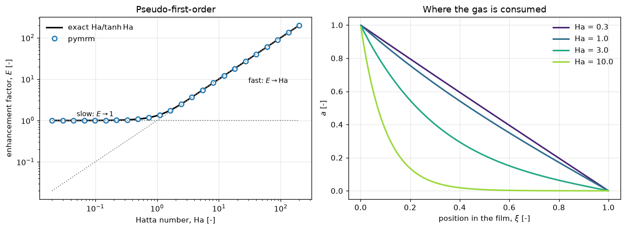

max relative error vs the exact solution: 6.337e-03

Second order — and what the approximations cost

Now the co-reactant is depleted inside the film. \(E\) can no longer exceed the instantaneous ceiling \(E_i\), and neither published formula is exact.

def vkh(ha, e_i):
    """Van Krevelen-Hoftijzer, solved for E by bisection."""
    def f(E):
        s = np.sqrt(max((e_i - E) / (e_i - 1.0), 0.0))
        return E - (ha * s / np.tanh(ha * s) if ha * s > 1e-12 else 1.0)
    return brentq(f, 1.0, e_i - 1e-12, xtol=1e-12)


def decoursey(ha, e_i):
    """DeCoursey's explicit approximation."""
    q = e_i - 1.0
    return -ha**2 / (2 * q) + np.sqrt(ha**4 / (4 * q**2) + e_i * ha**2 / q + 1.0)


film2 = Film(n_x=400, n_c=2)
E_I = [5.0, 20.0, 100.0]
ha2 = np.geomspace(0.05, 300.0, 55)
res = {}
for e_i in E_I:
    u_warm, rows = None, []
    for h in ha2:
        u_warm, E, ok = film2.solve_second_order(h, e_i, u_init=u_warm)
        rows.append((E if ok else np.nan, vkh(h, e_i), decoursey(h, e_i)))
    res[e_i] = np.array(rows)

fig, axes = plt.subplots(1, 2, figsize=(11.5, 4.3))
cols = plt.cm.plasma(np.linspace(0.15, 0.75, len(E_I)))
for e_i, c in zip(E_I, cols):
    r = res[e_i]
    axes[0].loglog(ha2, r[:, 0], color=c, lw=2.2, label=rf"$E_i$ = {e_i:.0f}")
    axes[0].loglog(ha2, r[:, 1], "--", color=c, lw=1.4)
    axes[0].loglog(ha2, r[:, 2], ":", color=c, lw=1.6)
    axes[0].axhline(e_i, color=c, lw=0.7, ls="-.", alpha=0.5)
    axes[1].semilogx(ha2, 100 * (r[:, 1] - r[:, 0]) / r[:, 0], "--", color=c, lw=1.6,
                     label=rf"VKH, $E_i$ = {e_i:.0f}")
    axes[1].semilogx(ha2, 100 * (r[:, 2] - r[:, 0]) / r[:, 0], ":", color=c, lw=2,
                     label=rf"DeCoursey, $E_i$ = {e_i:.0f}")

axes[0].loglog(ha2, ha2 / np.tanh(ha2), color="0.6", lw=1.2,
               label="pseudo-first-order")
axes[0].set_xlabel(r"$\mathrm{Ha}$ [-]"); axes[0].set_ylabel("$E$ [-]")
axes[0].set_title("solid pymrm · dashed VKH · dotted DeCoursey")
axes[0].legend(frameon=False, fontsize=8)
axes[1].axhline(0, color="k", lw=0.8)
axes[1].set_xlabel(r"$\mathrm{Ha}$ [-]")
axes[1].set_ylabel("approximation error [%]")
axes[1].set_title("Departure from the full solution")
axes[1].legend(frameon=False, fontsize=7, ncol=2)
fig.tight_layout(); plt.show()

for e_i in E_I:
    r = res[e_i]
    v = 100 * np.abs(r[:, 1] - r[:, 0]) / r[:, 0]
    d = 100 * np.abs(r[:, 2] - r[:, 0]) / r[:, 0]
    print(f"E_i = {e_i:5.0f}:  VKH max {v.max():5.1f}% (at Ha={ha2[v.argmax()]:6.2f})"
          f"   DeCoursey max {d.max():5.1f}% (at Ha={ha2[d.argmax()]:6.2f})")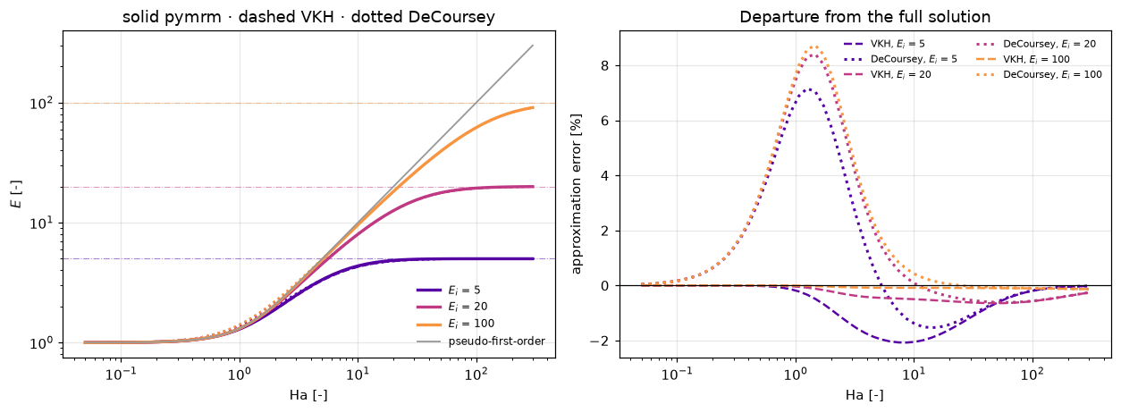

E_i =     5:  VKH max   2.1% (at Ha=  8.67)   DeCoursey max   7.2% (at Ha=  1.25)
E_i =    20:  VKH max   0.6% (at Ha= 50.99)   DeCoursey max   8.4% (at Ha=  1.47)
E_i =   100:  VKH max   0.1% (at Ha=300.00)   DeCoursey max   8.7% (at Ha=  1.47)

# The concentration profiles behind the three regimes.
fig, axes = plt.subplots(1, 3, figsize=(12.5, 3.7), sharey=True)
for ax, h, tag in zip(axes, [0.3, 3.0, 50.0],
                      ["slow: reaction happens in the bulk",
                       "fast: consumed inside the film",
                       "instantaneous: reaction plane"]):
    u, E, _ = film2.solve_second_order(h, 20.0)
    ax.plot(film2.x_c, u[:, 0], color="tab:blue", lw=2.2, label="$a$ (gas)")
    ax.plot(film2.x_c, u[:, 1], color="tab:red", lw=2.2, label="$b$ (co-reactant)")
    ax.set_title(f"Ha = {h:g},  E = {E:.2f}\n{tag}", fontsize=9)
    ax.set_xlabel(r"$\xi$ [-]")
axes[0].set_ylabel("dimensionless concentration [-]")
axes[0].legend(frameon=False)
fig.tight_layout(); plt.show()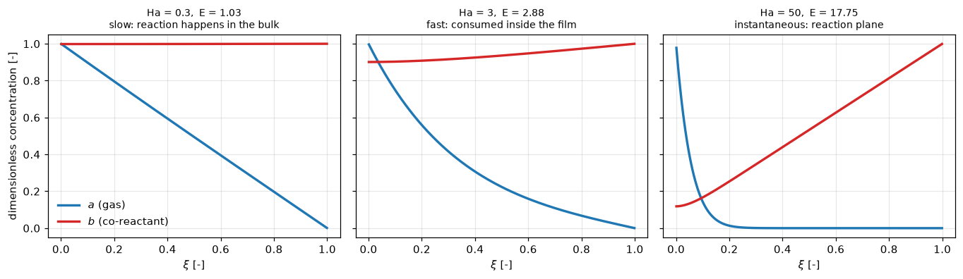

Validation

Four checks; none uses fitted data.

# 1. First order against the exact closed form.
print(f"1. max rel. error vs Ha/tanh(Ha)          : {err1:.3e}")

# 2. Grid convergence.
errs = []
for n in (100, 200, 400, 800):
    f = Film(n_x=n, n_c=1)
    errs.append(abs(f.solve_first_order(5.0)[1] - 5.0 / np.tanh(5.0))
                / (5.0 / np.tanh(5.0)))
order = np.log2(errs[-2] / errs[-1])
print(f"2. observed order of convergence          : {order:.2f}   (expected 2)")

# 3. Limiting behaviour of the second-order solution:
#    E -> 1 as Ha -> 0, and E -> E_i as Ha -> infinity.
lo = res[20.0][0, 0]
hi = res[20.0][-1, 0]
print(f"3. E at Ha={ha2[0]:.2f} (expect 1)            : {lo:.4f}")
print(f"   E at Ha={ha2[-1]:.0f} (expect E_i = 20)      : {hi:.4f}")

# 4. Second-order must reduce to pseudo-first-order when the co-reactant
#    is in large excess.
film_x = Film(n_x=400, n_c=2)
dev = []
for h in (0.5, 2.0, 10.0):
    _, E2, _ = film_x.solve_second_order(h, 1.0e6)
    dev.append(abs(E2 - h / np.tanh(h)) / (h / np.tanh(h)))
print(f"4. E_i -> inf reduces to first order, max dev: {max(dev):.3e}")

report_agreement("F3.1", {
    "first_order_max_rel_error": float(err1),
    "convergence_order": float(order),
    "limit_E_small_Ha": float(lo),
    "limit_E_large_Ha": float(hi),
    "excess_reduces_to_first_order": float(max(dev)),
    "vkh_max_error_pct": float(max(
        np.max(100 * np.abs(res[e][:, 1] - res[e][:, 0]) / res[e][:, 0])
        for e in E_I)),
    "decoursey_max_error_pct": float(max(
        np.max(100 * np.abs(res[e][:, 2] - res[e][:, 0]) / res[e][:, 0])
        for e in E_I)),
})

1. max rel. error vs Ha/tanh(Ha)          : 6.337e-03
2. observed order of convergence          : 3.07   (expected 2)
3. E at Ha=0.05 (expect 1)            : 1.0008
   E at Ha=300 (expect E_i = 20)      : 19.9683
4. E_i -> inf reduces to first order, max dev: 5.384e-06
Agreement metrics for F3.1:
  first_order_max_rel_error     = 0.0063367
  convergence_order             = 3.0719
  limit_E_small_Ha              = 1.0008
  limit_E_large_Ha              = 19.968
  excess_reduces_to_first_order = 5.384e-06
  vkh_max_error_pct             = 2.0769
  decoursey_max_error_pct       = 8.7204

{'page': 'F3.1',
 'metrics': {'first_order_max_rel_error': 0.006336733444486526,
  'convergence_order': 3.0719034053588943,
  'limit_E_small_Ha': 1.0008331631554483,
  'limit_E_large_Ha': 19.96831594054015,
  'excess_reduces_to_first_order': 5.384037445220569e-06,
  'vkh_max_error_pct': 2.076893245879678,
  'decoursey_max_error_pct': 8.72038368927803}}

What pymrm adds

For the pseudo-first-order case, nothing — and as on B1.1, that is the point. The closed form is exact; reproducing it to \(10^{-4}\) with second-order convergence is what licenses the second-order result, where no closed form exists.

For the second-order case, the error bar on the standard formulas. Van Krevelen–Hoftijzer and DeCoursey are used constantly in absorber design and almost always without a stated accuracy. Solving the film equations directly puts a number on both, across the whole \((\mathrm{Ha}, E_i)\) plane, and shows where they degrade — in the transition between the fast and instantaneous regimes, which is precisely the operating region of a real amine absorber.

The full solve is not expensive: a few hundred cells and a Newton iteration. There is no longer much reason to reach for the approximation when the equation itself is this cheap.

Reuse

Change	Where
Reversible reaction / equilibrium	extend rate and add the product as a third component
Surface renewal instead of a film	replace the steady BVP with a transient penetration solve (S4)
Non-depleted bulk, \(a(1) = a_b > 0\)	change d in the right-hand boundary dictionary
Gas-side resistance	make the interface a Robin condition instead of Dirichlet
Couple to a column	this is the local closure inside F2.1/F3.5

Related pages: F3.2 Van Krevelen–Hoftijzer · F3.3 DeCoursey · F3.5 CO₂–amine absorption · B1.1 Thiele (the same S3 equation with the boundary conditions swapped) · A4.9 Duncan–Toor.

References

Hatta, S. (1932). On the absorption velocity of gases by liquids. Technological Reports of Tôhoku University 10, 119–128.

Van Krevelen, D. W. and Hoftijzer, P. J. (1948). Kinetics of gas-liquid reactions. Part I. General theory. Recueil des Travaux Chimiques des Pays-Bas 67(7), 563–586. doi:10.1002/recl.19480670708

DeCoursey, W. J. (1974). Absorption with chemical reaction: development of a new relation for the Danckwerts model. Chemical Engineering Science 29(9), 1867–1872. doi:10.1016/0009-2509(74)85003-7

Danckwerts, P. V. (1970). Gas-Liquid Reactions. McGraw-Hill.