# Bootstrap: the pymrm this page was checked with, and the gallery files it was
# published with. Works in a checkout, in CI and on a fresh Colab VM.
GALLERY_REF = "gallery-2026.11.10.3"  # replaced by the release tag at publication
PYMRM = ">=3.3.0,<4"  # equals meta.yaml pymrm_min_version, up to the next major
PAGE = "F2.3-slurry-bubble-column-ft"  # equals the page directory

import os, sys, urllib.request
from pathlib import Path
_shared = next((p / "shared" for p in (Path.cwd(), *Path.cwd().parents)
                if (p / "shared" / "gallery_bootstrap.py").is_file()), None)
if _shared is None:
    _shared = (Path(os.environ.get("XDG_CACHE_HOME") or Path.home() / ".cache")
               / "pymrm-gallery" / GALLERY_REF)
    _shared.mkdir(parents=True, exist_ok=True)
    urllib.request.urlretrieve(
        "https://raw.githubusercontent.com/computational-chemical-engineering/"
        f"pymrm-gallery/{GALLERY_REF}/shared/gallery_bootstrap.py",
        _shared / "gallery_bootstrap.py")
sys.path.insert(0, str(_shared))
sys.modules.pop("gallery_bootstrap", None)
from gallery_bootstrap import setup
setup(PAGE, PYMRM, GALLERY_REF); # the semicolon stops the cell echoing the pathA Fischer–Tropsch slurry bubble column, and two typos that stop it working
sec:F
struct:S7
struct:S8
tier:T1
data:tier4
phase:gas-liquid-solid
Plug-flow large bubbles over a well-mixed slurry. The hydrodynamics are tested against measured holdup; the reactor reaches the published conversions only after two printed constants are corrected against the paper’s own results, and the gas contraction is read as a molar conversion.
A Fischer–Tropsch slurry bubble column, and two typos that stop it working
Catalog ID: F2.3 · Structures: S7 (multiphase coupling), S8 (reactor plus transport) · Tier: T1
A commercial Fischer–Tropsch slurry reactor is 7 m across and 30 m tall, and the gas inside it travels two different ways. Small bubbles drift with the slurry and stay long enough to equilibrate with it. Large bubbles rise through the column in plug flow, and they shrink as the syngas they carry is converted.
This page builds Maretto and Krishna’s (1999) model of that reactor. The hydrodynamics are checked against the paper’s measured holdup; the reactor is checked against the conversions and productivities the authors report, which it only approaches after two printed constants are corrected. The whole reactor, gas profiles and liquid concentrations together, is one Newton solve on pymrm operators, checked against an independent ODE route.
# Imports. The page's model.py is put on sys.path by setup().
import numpy as np
import matplotlib.pyplot as plt
from IPython.display import Markdown, display
from pymrm.checks import find_roots, observed_orders
from gallery_utils import load_data, load_meta, cite_data, Claims
from model import (PARAMS, ColumnSolution, Operating, SlurryColumn, hydrodynamics,
                   reactor_ode)

plt.rcParams.update({"figure.dpi": 110, "axes.grid": True, "grid.alpha": 0.3})
claims = Claims(PAGE.split("-")[0])
EPS = np.finfo(float).eps
BREAK = []   # (injected defect, claim, clean value, broken value, caught)


def brk(row, metric, broken):
    """One injected defect: ``broken`` is what claim ``metric`` becomes with it."""
    caught = claims.breaks(row, metric, broken)
    BREAK.append((row, metric, claims[metric], broken, caught))
Background
The two-bubble-class picture comes from F1.4: above the regime transition a churn-turbulent column carries a dilute phase of fast large bubbles and a dense phase of slurry with small bubbles entrained in it.
For a slurry reactor two things change. Catalyst particles promote coalescence, which destroys small bubbles: the dense-phase holdup falls as solids are added, and by about 38 vol % solids the small-bubble population is gone (the paper’s eq. 7). Pressure works the other way: a commercial reactor runs at 30 bar, where the gas is 7 kg/m³ rather than 1.3, which delays the transition and puts more gas into small bubbles (eq. 11).
The reactor model couples three things: large bubbles in plug flow, small bubbles and slurry treated as well mixed, and Fischer–Tropsch kinetics on cobalt. A distributed phase exchanging with lumped phases is the S7/S8 structure.
The published model
Hydrodynamics (eqs. 6 to 11). Small-bubble holdup falls linearly with the solids fraction \(\varepsilon_s\) and rises with gas density; their rise velocity grows with \(\varepsilon_s\):
\[ \varepsilon_{df} = \varepsilon_{df,\mathrm{ref}} \left(\frac{\rho_G}{\rho_{G,\mathrm{ref}}}\right)^{0.48} \left(1 - \frac{0.7}{\varepsilon_{df,\mathrm{ref}}}\varepsilon_s\right), \qquad V_{\mathrm{small}} = V_{\mathrm{small,ref}} + 0.8\,\varepsilon_s, \]
\[ U_{df} = \varepsilon_{df} V_{\mathrm{small}},\qquad \varepsilon_b = 0.3\,\min(D_T, 1)^{-0.18}\,(U-U_{df})^{0.58},\qquad \varepsilon = \varepsilon_b + \varepsilon_{df}(1-\varepsilon_b), \]
with \(\varepsilon_{df,\mathrm{ref}} = 0.27\) and \(V_{\mathrm{small,ref}} = 0.095\) m/s for paraffin oil. Eq. 9’s coefficient is 0.3 here, against 0.268 in F1.4’s eq. 19 (Krishna and Ellenberger 1996, fitted to gas-liquid systems); this paper states eq. 9 for slurries above \(\varepsilon_s = 0.16\). The diameter dependence is capped at \(D_T = 1\) m.
Mass transfer is tied to holdup (eqs. 13, 14): \((k_La)_{\mathrm{large}} = 0.5\,\varepsilon_b\sqrt{D_L/D_{L,\mathrm{ref}}}\) and \((k_La)_{\mathrm{small}} = 1.0\,\varepsilon_{df}\sqrt{D_L/D_{L,\mathrm{ref}}}\), with \(D_{L,\mathrm{ref}} = 2\times10^{-9}\) m²/s and the solubility \(m\) defined by \(c_G = m\,c_L\).
Kinetics are Yates and Satterfield’s on cobalt (eqs. 1 to 3), with the partial pressures in equilibrium with the liquid:
\[-R = \frac{a\,p_{\mathrm{H}_2}p_{\mathrm{CO}}}{(1+b\,p_{\mathrm{CO}})^2}.\]
Reactor (eqs. 15 to 21). Large bubbles in plug flow at superficial velocity \(U - U_{df}\), small bubbles and slurry well mixed:
\[ \frac{d}{dz}\Big[(U-U_{df})\,c_{G,i}\Big] = -(k_La)_{i,\mathrm{large}}\left(\frac{c_{G,i}}{m_i} - c_{L,i}\right), \qquad U_{df}\big(c^{\,i}_{G,i} - c_{G,i}^{\,\mathrm{small}}\big) = (k_La)_{i,\mathrm{small}}\left(\frac{c_{G,i}^{\,\mathrm{small}}}{m_i} - c_{L,i}\right) H, \]
and per species a liquid balance (eqs. 19 and 20): the large-bubble transfer integrated over the height, plus the small-bubble transfer, equals \(H\,\nu_i\,w_{\mathrm{cat}}\,R\), with \(\nu_{\mathrm{CO}} = 1\) and \(\nu_{\mathrm{H_2}} = 2\) and \(w_{\mathrm{cat}} = \varepsilon_L\varepsilon_s\rho_p\) the catalyst per reactor volume. The large bubbles contract as syngas converts (eq. 21):
\[U-U_{df} = (U^i-U_{df})(1+\alpha\,\chi),\qquad \alpha = -0.648 .\]
What \(\chi\) is. The paper calls it the syngas conversion. Read as the molar conversion of the large-bubble syngas, \(\chi = 1 - (U-U_{df})\,r/(U^i-U_{df})\) with \(r = \sum_i c_{G,i}/\sum_i c^{\,i}_{G,i}\), eq. 21 closes to \((U-U_{df})/(U^i-U_{df}) = (1+\alpha)/(1+\alpha r)\). Read as \(\chi = 1 - r\), a concentration ratio, it gives \(1 + \alpha(1-r)\) instead. The page uses the molar reading, the only one under which the conversion leaving the column is the conversion eq. 21 was evaluated at, and measures what the other gives.
| symbol | meaning | in the code |
|---|---|---|
| \(c_{G,i}/c^{\,i}_{G,i}\) | large-bubble gas, relative to the feed | y, shape (n, 2) |
| \(m_i c_{L,i}/c^{\,i}_{G,i}\) | liquid, as the gas in equilibrium with it | x, shape (2,) |
| \((U-U_{df})\,c_{G,i}/[(U^i-U_{df})c^{\,i}_{G,i}]\) | large-bubble molar flux | q = s(r) y |
| \((k_La)_i/m_i\) | large- and small-bubble exchange | Operating.K, Operating.K_s |
| \(\varepsilon_L\varepsilon_s\rho_p\) | catalyst per reactor volume | Operating.cat |
Parameters and assumptions
Table 1 of the paper: \(T\) = 240 °C, \(P\) = 30 bar, \(D_T\) = 7 m, \(H\) = 30 m, catalyst partial density 647 kg/m³, contraction factor \(\alpha = -0.648\) at 5 vol % inert. Solubilities \(m_{\mathrm{CO}} = 2.478\) and \(m_{\mathrm{H}_2} = 2.964\), diffusivities \(45.5\) and \(17.2 \times 10^{-9}\) m²/s. Feed H₂/CO = 2, the consumption ratio, so CO, H₂ and syngas conversions coincide. The feed is an ideal gas at \(P\) and \(T\) with 5 % inert.
Assumptions taken from the paper: isothermal, no particle or liquid-solid resistance, \(U_{df}\) constant along the height, only the large bubbles contract. Assumptions of this page: the liquid outflow term \(A U_L^o c_L\) of eqs. 19 and 20 is dropped because \(U_L^o\) is not in Table 1 (its size is measured in the Results); eqs. 19 and 20 print the rate without a catalyst concentration, and it is taken per kg of catalyst with \(\varepsilon_L\varepsilon_s\rho_p\) kg per m³ of reactor.
Two printed constants are corrected, each against the paper’s own reported results (shown in the Results):
- Eq. 2 prints the prefactor \(a = 8.8533\times10^{3}\) mol/(s·kg\(_{cat}\)·bar²). It is used as \(8.8533\times10^{-3}\).
- Eq. 1 labels its rate \(-R_{\mathrm{CO+H_2}}\), but eqs. 19 and 20 put it into the CO balance with coefficient 1 and the H₂ balance with 2, and the paper says \(R_{\mathrm{H_2}} = 2R_{\mathrm{CO}}\). It is used as the CO rate.
p = PARAMS
print(f"T = {p['T'] - 273.15:.0f} C, P = {p['P'] / 1e5:.0f} bar, D_T = {p['DT']} m, "
      f"H = {p['H']} m, rho_p = {p['rho_p']} kg/m3, alpha = {p['alpha']}, "
      f"inert = {p['inert']}")
print(f"m = {p['m']}, D_L = {p['D_L']} m2/s, a = {p['a_pre']:.4e} (printed 8.8533e+03), "
      f"rate read as CO (nu = {p['nu']})")
N_REP = 1600          # cells over the 30 m height for every reported reactor number
PAPER = dict(conv_U012=0.96, conv_U040=0.63,          # section 5, eps_s = 0.30
             prod_U012=1200.0, prod_U040=2640.0)      # t C1/day, same runs
M_CH2 = 12.011 + 2 * 1.008                           # g/mol, the C1 unit of the products
T = 240 C, P = 30 bar, D_T = 7.0 m, H = 30.0 m, rho_p = 647.0 kg/m3, alpha = -0.648, inert = 0.05
m = (2.478, 2.964), D_L = (4.55e-08, 1.72e-08) m2/s, a = 8.8533e-03 (printed 8.8533e+03), rate read as CO (nu = (1.0, 2.0))The data
Markers digitised from Figure 2: total gas holdup against superficial velocity at three slurry concentrations in a 0.10 m column at ambient conditions. The maintainer reviewed the extraction: where markers overlap the shape detector picks the wrong glyph, so series identity comes from which curve a marker sits on, not from its matched shape. Detections inside the merged cluster at the origin are carried with resolved = no and an empty eps_s and excluded from every number below. The figure also carries the authors’ model curves, which were not extracted.
obs = load_data("maretto-krishna-1999-fig2.csv", page=PAGE)
meta = load_meta("maretto-krishna-1999-fig2.csv", page=PAGE)


def data_counts(use_resolved=True):
    """Rows, resolved markers and cluster detections; ``use_resolved`` False ignores the flag."""
    keep = (obs.resolved == "yes") if use_resolved else np.ones(len(obs), bool)
    return len(obs), int(keep.sum()), int((~keep).sum())


n_rows, n_res, n_clu = data_counts()
res = obs[obs.resolved == "yes"].copy()
print(f"{n_rows} rows: {n_res} resolved, {n_clu} in the merged cluster")
for s, g in res.groupby("eps_s"):
    print(f"   eps_s = {s:4.2f}   n = {len(g):3d}   U {g.U_m_s.min():.3f}-{g.U_m_s.max():.3f} m/s"
          f"   eps {g.eps_total.min():.3f}-{g.eps_total.max():.3f}")
print(f"\n{cite_data(meta)}")
print(f"review: {meta['review']['verdict']}")
claims.exact("data_rows", n_rows, structural=True,
             note="the length of the committed CSV; no model defect can change it")
claims.exact("data_resolved", n_res)
claims.exact("data_cluster", n_clu)
115 rows: 95 resolved, 20 in the merged cluster
eps_s = 0.00 n = 13 U 0.009-0.491 m/s eps 0.156-0.483
eps_s = 0.16 n = 46 U 0.006-0.497 m/s eps 0.112-0.386
eps_s = 0.35 n = 36 U 0.021-0.471 m/s eps 0.069-0.306
Maretto, C.; Krishna, R. (1999) — Catalysis Today 52(2-3) 279-289 — doi:10.1016/S0920-5861(99)00082-6 — digitised from Figure 2, journal page 282
review: positions good, series assignment needed fixing, cluster to be reported not droppedPyMRM implementation
The reactor is one distributed phase exchanging with two lumped ones.
Large bubbles. Their balance is written for the molar flux. In the dimensionless unknowns y the flux is q = s(r) y, with s the contraction of eq. 21, so first-order upwind with unit velocity on q (construct_convflux_upwind, construct_div with nu = 0) carries the upstream cell’s \((U-U_{df})c\) through every face. The scheme is conservative for any velocity profile, and the operator is constant: it is assembled once. The inlet is \(q = 1\) ({"a": 0, "b": 1, "d": 1}), the outlet {"outflow": True}, where gas leaves with the last cell’s flux and no condition is imposed. The state has shape (n, 2), height first and the species CO, H₂ last.
Small bubbles close in one line (eqs. 17, 18), and are substituted into the two liquid balances (eqs. 19, 20). The unknown vector is the 2n gas values followed by the 2 liquid values, and pymrm.newton solves the whole system with an exact sparse Jacobian: the constant convection block times the 2 × 2 blocks of \(\partial q/\partial y\) per cell, the exchange diagonal, and the dense coupling rows of the height integral. No fixed-point loop over the liquid concentrations is needed. The exit is read on the outlet face with compute_boundary_values.
model.py holds this as Operating (everything fixed at one operating point), SlurryColumn (operators, residual, Jacobian, solve) and ColumnSolution (conversions). reactor_ode is the independent route used in the Validation.
LOG = []   # every reported solve: (case, solution)


def solve(U, eps_s=0.30, n=N_REP, op_kw=None, record=True, tol=1e-12, maxfev=50,
          check=True, **col_kw):
    """One reactor solve; reported solves are logged for the balance checks."""
    sol = SlurryColumn(Operating(U, eps_s, **(op_kw or {})), n, **col_kw).solve(
        tol=tol, maxfev=maxfev, check=check)
    if record:
        LOG.append(((U, eps_s, n, tuple(sorted((op_kw or {}).items())),
                     tuple(sorted(col_kw.items()))), sol))
    return sol


def conv(U, eps_s=0.30, read="face", **kw):
    """Syngas conversion, or nan where newton does not converge (a defect row)."""
    try:
        return solve(U, eps_s, **kw).syngas_conversion(read)
    except RuntimeError:
        return np.nan


demo = solve(0.40)
col = demo.col
print(f"{col.n} cells, {2 * col.n + 2} unknowns, Jacobian nnz "
      f"{col.residual(demo.u)[1].nnz}; newton from y = 1, x = 0.05 converges, "
      f"largest residual below 1e-10 (here {demo.resid:.1e})")
1600 cells, 3202 unknowns, Jacobian nnz 19200; newton from y = 1, x = 0.05 converges, largest residual below 1e-10 (here 4.8e-14)Results
Hydrodynamics against Figure 2
The figure’s column is 0.10 m at ambient conditions, so eq. 11’s pressure factor is 1 and \(\min(D_T, 1)^{-0.18} = 0.10^{-0.18}\): the only place on this page where the diameter term does anything. The comparison uses the same hydrodynamics function as the reactor. Markers with \(U \le 2U_{df}\) are left out: eq. 9 describes the churn-turbulent regime, and the factor 2 is this page’s choice of where that regime has begun. The \(\varepsilon_s = 0\) markers jump from 0.014 to 0.140 m/s, so any cut in between selects the same eight; the break table moves the cut to \(U_{df}\) and to \(6U_{df}\).
FIG = dict(d_t=0.10, rho_g=PARAMS["rho_g_ref"])
SERIES = (0.0, 0.16, 0.35)
TAG = {0.0: "0", 0.16: "016", 0.35: "035"}


def holdup_stats(factor=2.0, rho_g=FIG["rho_g"], **over):
    """Per series: (U/(factor U_df) of every marker, mean |dev|, mean dev, n used)."""
    out = {}
    for s, g in res.groupby("eps_s"):
        h = hydrodynamics(g.U_m_s.values, s, d_t=FIG["d_t"], rho_g=rho_g, **over)
        ratio = g.U_m_s.values / (factor * h["U_df"])
        v = ratio > 1.0
        dev = h["eps"][v] / g.eps_total.values[v] - 1.0
        out[float(s)] = (ratio, float(np.abs(dev).mean()), float(dev.mean()), int(v.sum()))
    return out


HS = holdup_stats()
fig, ax = plt.subplots(1, 2, figsize=(12.6, 4.4))
cols = {0.0: "tab:red", 0.16: "tab:green", 0.35: "tab:blue"}
UU = np.linspace(0.001, 0.5, 300)
for s, g in res.groupby("eps_s"):
    h = hydrodynamics(UU, s, **FIG)
    ax[0].plot(UU, h["eps"], color=cols[s], lw=1.9, label=rf"model, $\epsilon_s$ = {s}")
    ax[0].plot(g.U_m_s, g.eps_total, "o", ms=4.5, mfc="none", mew=1.2, color=cols[s])
    ax[0].axvline(2 * h["U_df"], color=cols[s], ls=":", lw=1.0)
    v = HS[s][0] > 1.0
    hv = hydrodynamics(g.U_m_s.values[v], s, **FIG)
    ax[1].plot(g.U_m_s.values[v], (hv["eps"] / g.eps_total.values[v] - 1) * 100, "o", ms=4.5,
               mfc="none", mew=1.2, color=cols[s], label=rf"$\epsilon_s$ = {s}")
ax[0].set(xlabel="superficial gas velocity $U$ [m/s]", ylabel=r"total gas holdup $\epsilon$",
          title="hydrodynamics against Figure 2\n(dotted: $2U_{df}$, below which markers are not used)",
          xlim=(0, 0.52), ylim=(0, 0.55))
ax[0].legend(fontsize=8)
ax[1].axhline(0, color="k", lw=1.1)
ax[1].set(xlabel="superficial gas velocity $U$ [m/s]", ylabel="(model - data)/data [%]",
          title="residuals of the markers used", ylim=(-40, 40))
ax[1].legend(fontsize=8)
fig.tight_layout(); plt.show()

print("holdup at U > 2 U_df (0.10 m column, ambient gas):")
for s in SERIES:
    ratio, mad, bias, n_v = HS[s]
    udf = hydrodynamics(0.1, s, **FIG)["U_df"]
    print(f"   eps_s = {s:4.2f}   U_df = {udf:.4f} m/s   n = {n_v:3d}   "
          f"mean |dev| {mad * 100:4.1f} %   bias {bias * 100:+5.1f} %")
    claims.count(f"n_used_eps_s_{TAG[s]}", ratio, 1.0, min_margin=0.02,
                 note="markers above 2 U_df; margin = nearest marker to the cut")
    claims.value(f"holdup_mad_eps_s_{TAG[s]}", mad, rtol=1e-6)
    claims.value(f"holdup_bias_eps_s_{TAG[s]}", bias, rtol=1e-6)
n_used = sum(HS[s][3] for s in SERIES)
print(f"{n_used} markers used, one set of constants, nothing fitted")
claims.exact("n_used_total", n_used)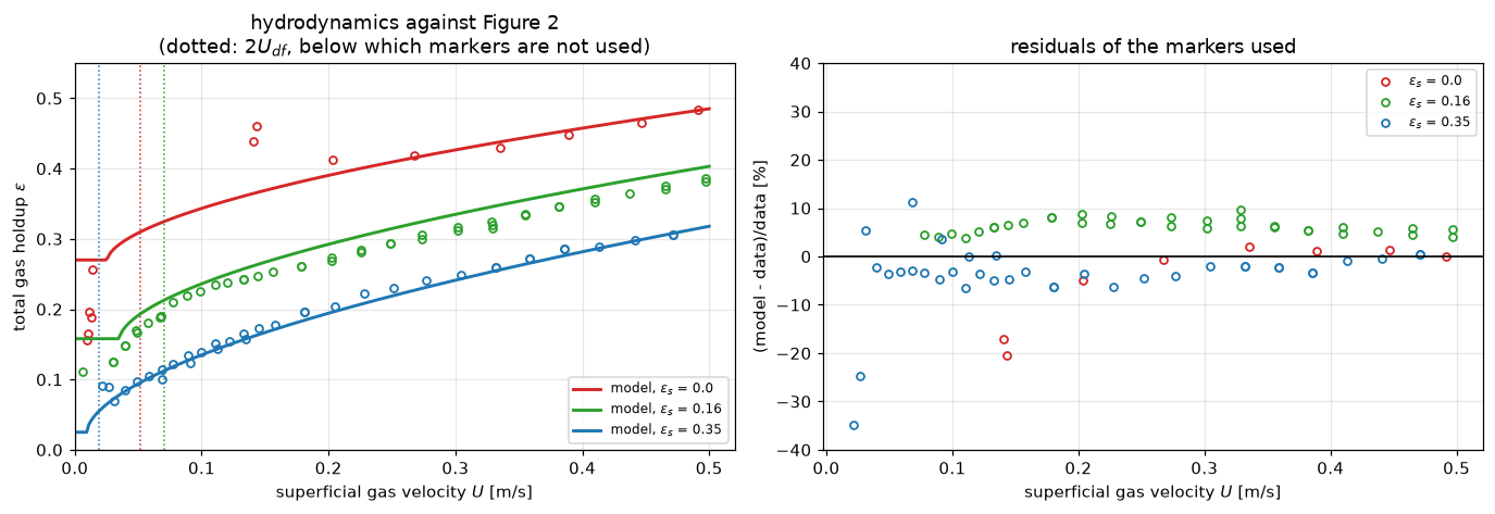
holdup at U > 2 U_df (0.10 m column, ambient gas):
   eps_s = 0.00   U_df = 0.0257 m/s   n =   8   mean |dev|  5.9 %   bias  -4.8 %
   eps_s = 0.16   U_df = 0.0352 m/s   n =  35   mean |dev|  6.3 %   bias  +6.3 %
   eps_s = 0.35   U_df = 0.0094 m/s   n =  36   mean |dev|  4.9 %   bias  -3.7 %
79 markers used, one set of constants, nothing fitted
Eq. 9’s coefficient: 0.3 here, 0.268 in F1.4. The same markers, the same cut, the two coefficients:
HS268 = holdup_stats(C9=0.268)
print(f"   {'eps_s':>6}{'C = 0.300':>12}{'C = 0.268':>12}")
for s in SERIES:
    print(f"   {s:6.2f}{HS[s][1] * 100:11.1f} %{HS268[s][1] * 100:11.1f} %")
    claims.value(f"holdup_mad_C0268_eps_s_{TAG[s]}", HS268[s][1], rtol=1e-6)
eps_s C = 0.300 C = 0.268
0.00 5.9 % 8.5 %
0.16 6.3 % 1.5 %
0.35 4.9 % 12.4 %0.3 is the more consistent of the two across the three concentrations. 0.268 fits \(\varepsilon_s = 0.16\) better and is clearly worse at 0.35, the range this paper’s eq. 9 is stated for.
The reactor
Conversion at \(\varepsilon_s = 0.30\) over the paper’s velocity range, on 1600 cells (the grid error is measured in the Validation):
U_LIST = (0.12, 0.20, 0.30, 0.40)
UTAG = {0.12: "U012", 0.20: "U020", 0.30: "U030", 0.40: "U040"}
X030 = {U: conv(U) for U in U_LIST}
print("reactor, eps_s = 0.30:")
for U in U_LIST:
    print(f"   U = {U:.2f} m/s   conversion = {X030[U] * 100:5.1f} %")
    claims.value(f"conversion_{UTAG[U]}", X030[U], rtol=1e-4)
print(f"   the paper reports {PAPER['conv_U012'] * 100:.0f} % at U = 0.12 and "
      f"{PAPER['conv_U040'] * 100:.0f} % at U = 0.40")

# The paper's productivities for the same two runs, converted back to conversion
# with this page's feed (ideal gas at P, T, 5 % inert, H2/CO = 2) and area.
area = np.pi * PARAMS["DT"] ** 2 / 4


def implied_conversion(prod_t_day, U, **over):
    """Conversion that a productivity in t C1/day implies for this page's feed."""
    op = Operating(U, 0.30, **over)
    return prod_t_day * 1e6 / (86400 * M_CH2 * U * area * op.c_in[0])


imp = {U: implied_conversion(PAPER[k], U) for U, k in ((0.12, "prod_U012"), (0.40, "prod_U040"))}
print(f"   its productivities, {PAPER['prod_U012']:.0f} and {PAPER['prod_U040']:.0f} t C1/day, imply "
      f"{imp[0.12] * 100:.1f} % and {imp[0.40] * 100:.1f} % for this feed")
claims.value("paper_implied_conversion_U012", imp[0.12], rtol=1e-6)
claims.value("paper_implied_conversion_U040", imp[0.40], rtol=1e-6)


def gaps(**over):
    """Model against the conversions the paper's productivities imply (points / 100)."""
    rec = not over
    return dict(gap_implied_U012=implied_conversion(PAPER["prod_U012"], 0.12, **over)
                - conv(0.12, op_kw=over, record=rec),
                gap_implied_U040=conv(0.40, op_kw=over, record=rec)
                - implied_conversion(PAPER["prod_U040"], 0.40, **over))


GP = gaps()
print(f"   model {GP['gap_implied_U012'] * 100:.1f} points below at U = 0.12, "
      f"{GP['gap_implied_U040'] * 100:.1f} points above at U = 0.40")
for k, v in GP.items():
    claims.value(k, v, rtol=1e-4)
reactor, eps_s = 0.30:
U = 0.12 m/s conversion = 93.3 %
U = 0.20 m/s conversion = 89.2 %
U = 0.30 m/s conversion = 79.3 %
U = 0.40 m/s conversion = 65.7 %
the paper reports 96 % at U = 0.12 and 63 % at U = 0.40
its productivities, 1200 and 2640 t C1/day, imply 96.3 % and 63.5 % for this feed
model 3.0 points below at U = 0.12, 2.2 points above at U = 0.40fig, ax = plt.subplots(1, 2, figsize=(12.4, 4.3))
US = np.linspace(0.12, 0.40, 8)
for es, c in ((0.20, "tab:blue"), (0.30, "tab:green"), (0.35, "tab:red")):
ax[0].plot(US, [conv(u, es) * 100 for u in US], "o-", color=c, lw=1.9, ms=4,
label=rf"$\epsilon_s$ = {es}")
ax[0].plot(US, [conv(u, law="concentration") * 100 for u in US], "--", color="tab:green",
lw=1.2, label=r"$\epsilon_s$ = 0.30, $\chi = 1 - r$ in eq. 21")
ax[0].plot([0.12, 0.40], [PAPER["conv_U012"] * 100, PAPER["conv_U040"] * 100], "k*", ms=14,
label=r"paper, $\epsilon_s$ = 0.30")
ax[0].set(xlabel="inlet superficial gas velocity $U$ [m/s]", ylabel="syngas conversion [%]",
ylim=(0, 105), title="conversion falls as throughput rises")
ax[0].legend(fontsize=8)
r = solve(0.30)
ax[1].plot(r.col.z_c, r.y[:, 0], lw=2, label="CO, $c_G/c_G^i$")
ax[1].plot(r.col.z_c, r.y[:, 1], lw=2, label="H$_2$, $c_G/c_G^i$")
ax[1].plot(r.col.z_c, r.s, "k--", lw=1.5, label="$(U-U_{df})/(U^i-U_{df})$")
ax[1].axhline(r.x[0], color="tab:blue", ls=":", lw=1)
ax[1].axhline(r.x[1], color="tab:orange", ls=":", lw=1)
ax[1].set(xlabel="height $z$ [m]", ylabel="relative to the inlet",
title="large bubbles, $U$ = 0.30 m/s, $\\epsilon_s$ = 0.30\n(dotted: the liquid, as equilibrium gas)")
ax[1].legend(fontsize=8)
fig.tight_layout(); plt.show()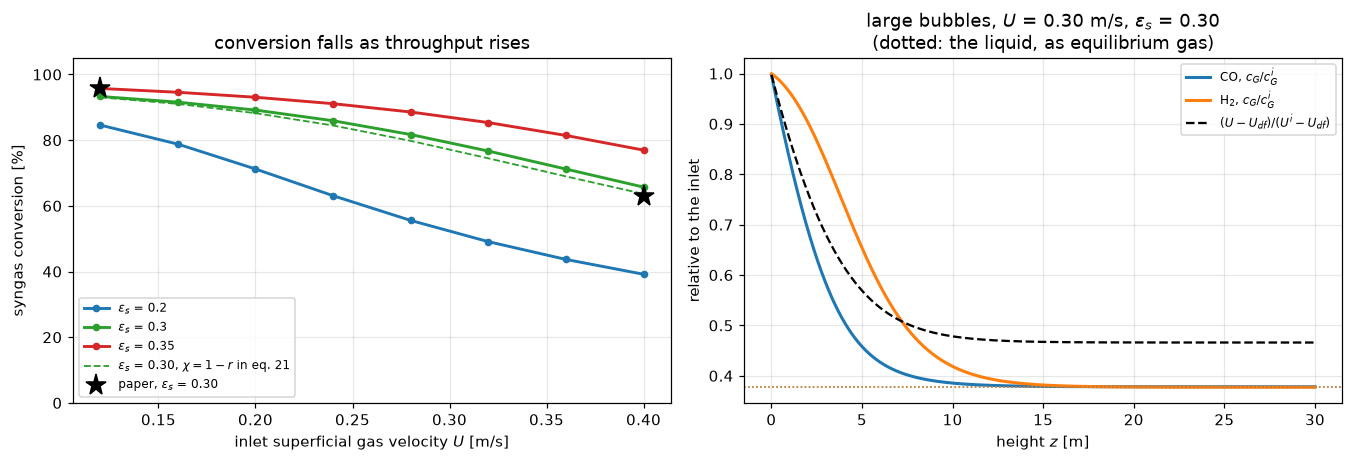
x_conc40 = conv(0.40, law="concentration")   # the other reading of eq. 21, see below
display(Markdown(
    "The model gives 93.3 % at $U$ = 0.12 m/s and 65.7 % at 0.40, against the 96 % and "
    "63 % the paper reports. The paper's productivities for the same runs imply "
    "96.3 % and 63.5 % with this page's feed, which confirms the feed basis (ideal gas "
    "at 30 bar and 240 °C, 5 % inert, a 7 m column) and the CH₂ unit of \"t C1\". The "
    "model sits 3.0 percentage points below at low velocity, which this page does not "
    "close, and 2.2 above at high velocity, where the other reading of eq. 21 (below) "
    f"gives {x_conc40 * 100:.1f} %."))
The model gives 93.3 % at \(U\) = 0.12 m/s and 65.7 % at 0.40, against the 96 % and 63 % the paper reports. The paper’s productivities for the same runs imply 96.3 % and 63.5 % with this page’s feed, which confirms the feed basis (ideal gas at 30 bar and 240 °C, 5 % inert, a 7 m column) and the CH₂ unit of “t C1”. The model sits 3.0 percentage points below at low velocity, which this page does not close, and 2.2 above at high velocity, where the other reading of eq. 21 (below) gives 63.6 %.
The two corrected constants, and what the alternatives give
Eq. 2 at 240 °C and the feed partial pressures, and each decade of the prefactor with each reading of eq. 1, against the paper:
EXPONENTS = (3, -2, -3, -4)
READINGS = (("CO", (1.0, 2.0)), ("syngas", (1 / 3, 2 / 3)))


def decade_table(mantissa=8.8533, record=True, **over):
    """Conversion at U = 0.12 and 0.40 for each prefactor decade and rate reading."""
    out = {}
    for e in EXPONENTS:
        for lab, nu in READINGS:
            kw = {**over, "a_pre": mantissa * 10.0 ** e, "nu": nu}
            for U in (0.12, 0.40):
                out[f"conversion_a{e:+d}_{lab}_{UTAG[U]}"] = conv(U, op_kw=kw, record=record)
    return out


def rate_metrics(**over):
    """Eq. 1 at the feed (x = 1) for the corrected and the printed prefactor, and the
    mean CO rate the paper's 96 % at U = 0.12 needs, per kg of catalyst."""
    op = Operating(0.12, 0.30, **over)
    feed = op.liquid_sink(np.ones(2))[2]
    need = PAPER["conv_U012"] * op.U * op.c_in[0] / (op.p["H"] * op.cat)
    return dict(rate_feed_corrected=feed, rate_feed_printed=feed * 1e6,
                rate_needed_U012=need, rate_feed_over_needed=feed / need)


RM = rate_metrics()
print(f"rate at the feed, 9.5 bar CO and 19 bar H2: {RM['rate_feed_corrected']:.2e} "
      f"mol CO/(s kg_cat) with 8.8533e-3, {RM['rate_feed_printed']:.2e} with the printed 8.8533e+3")
print(f"mean CO rate the paper's 96 % at U = 0.12 needs: {RM['rate_needed_U012']:.2e} mol CO/(s kg_cat)")
for k, v in RM.items():
    claims.value(k, v, rtol=1e-6)
def rate_factor(**over):
    """Factor on the prefactor ``a`` that makes the model give the paper's 96 % at
    U = 0.12: the one root on 1 <= factor <= 4 (nan when the range holds none)."""
    a0 = {**PARAMS, **over}["a_pre"]
    out = find_roots(lambda f: conv(0.12, op_kw={**over, "a_pre": f * a0}, record=False)
                     - PAPER["conv_U012"], 1.0, 4.0, n_scan=12, log=True)
    if len(out["roots"]) > 1 or out["failed"]:
        raise RuntimeError(f"rate factor: {out['message']}")
    return dict(rate_factor_for_96pct_U012=out["roots"][0] if out["roots"] else np.nan)


RF = rate_factor()
print(f"prefactor scaled by {RF['rate_factor_for_96pct_U012']:.2f} gives the paper's 96 % "
      f"at U = 0.12 (one root on 1 to 4); 1.8e-2 at the feed is no rate this page computes")
claims.value("rate_factor_for_96pct_U012", RF["rate_factor_for_96pct_U012"], rtol=1e-4)
DT_TAB = decade_table()
print(f"\n   {'prefactor a':>14}{'rate is':>9}{'conv U=0.12':>13}{'conv U=0.40':>13}")
for e in EXPONENTS:
    for lab, _nu in READINGS:
        c1, c4 = DT_TAB[f"conversion_a{e:+d}_{lab}_U012"], DT_TAB[f"conversion_a{e:+d}_{lab}_U040"]
        print(f"   {8.8533 * 10.0 ** e:14.4e}{lab:>9}{c1 * 100:12.1f}%{c4 * 100:12.1f}%")
print(f"   {'paper':>14}{'':>9}{PAPER['conv_U012'] * 100:12.1f}%{PAPER['conv_U040'] * 100:12.1f}%")
for k, v in DT_TAB.items():
    claims.value(k, v, rtol=1e-4)
rate at the feed, 9.5 bar CO and 19 bar H2: 1.58e-02 mol CO/(s kg_cat) with 8.8533e-3, 1.58e+04 with the printed 8.8533e+3
mean CO rate the paper's 96 % at U = 0.12 needs: 5.45e-03 mol CO/(s kg_cat)
prefactor scaled by 1.83 gives the paper's 96 % at U = 0.12 (one root on 1 to 4); 1.8e-2 at the feed is no rate this page computes
prefactor a rate is conv U=0.12 conv U=0.40
8.8533e+03 CO 99.6% 99.9%
8.8533e+03 syngas 99.6% 99.9%
8.8533e-02 CO 98.5% 97.9%
8.8533e-02 syngas 97.3% 94.5%
8.8533e-03 CO 93.3% 65.7%
8.8533e-03 syngas 72.8% 24.3%
8.8533e-04 CO 26.9% 7.4%
8.8533e-04 syngas 9.2% 2.5%
paper 96.0% 63.0%The prefactor. As printed, \(8.8533\times10^{3}\) makes the rate at the feed 1.6e4 mol CO/(s·kg\(_{cat}\)), \(10^6\) times the 1.6e-2 of \(8.8533\times10^{-3}\); the catalyst then consumes whatever mass transfer delivers and the conversion is 99.6 % and 99.9 %, nearly independent of throughput. Only the \(10^{-3}\) decade, read as the CO rate, comes near both published values; one decade either way misses one of them by tens of points. The rate at the feed, 1.6e-2, is 2.9 times the mean CO rate the 96 % needs (5.4e-3), as it must be: the liquid sits well below the feed partial pressures.
The reading of eq. 1. As a syngas rate (one third of it CO) the model gives 72.8 % and 24.3 %; as the CO rate, which is how eqs. 19 and 20 use it, 93.3 % and 65.7 %. Neither correction is a fitted number: each is a discrete choice between stated alternatives.
What the contraction does
At 100 % conversion eq. 21 shrinks the large-bubble flow to \(1+\alpha\) = 0.352 of its inlet value. With 5 % inert, \(\alpha = -0.648\) means 0.318 mol of gaseous product per mole of syngas converted, against 1/3 if all the water of CO + 2H₂ → (CH₂) + H₂O left as vapour and the hydrocarbon as liquid.
ALPHA = PARAMS["alpha"]


def contraction_metrics(**over):
    """At U = 0.40: exit flow and conversion of the large bubbles, the two readings."""
    s_m = solve(0.40, op_kw=over, record=not over)
    s_c = solve(0.40, op_kw=over, record=not over, law="concentration")
    op = s_m.col.op
    r_c = float(s_c.q_out @ op.w / s_c.s[-1])      # c/c_in on the outlet face
    out = dict(products_per_syngas=(op.p["alpha"] + 1 - op.p["inert"]) / (1 - op.p["inert"]),
               large_bubble_conversion_U040=s_m.large_bubble_conversion(),
               large_bubble_exit_flow_U040=1 + op.p["alpha"] * s_m.large_bubble_conversion(),
               concentration_reading_chi_gap_U040=s_c.large_bubble_conversion() - (1 - r_c))
    for U in (0.12, 0.40):
        xm = conv(U, op_kw=over, record=not over)
        xc = conv(U, op_kw=over, record=not over, law="concentration")
        x0 = conv(U, op_kw={**over, "alpha": 0.0}, record=not over)
        out[f"conversion_concentration_reading_{UTAG[U]}"] = xc
        out[f"conversion_no_contraction_{UTAG[U]}"] = x0
        out[f"contraction_worth_{UTAG[U]}"] = xm - x0
        out[f"reading_gap_{UTAG[U]}"] = xm - xc
    return out


CM = contraction_metrics()
XC = {U: CM[f"conversion_concentration_reading_{UTAG[U]}"] for U in (0.12, 0.40)}
X0 = {U: CM[f"conversion_no_contraction_{UTAG[U]}"] for U in (0.12, 0.40)}
print(f"gaseous product per mole of syngas converted: {CM['products_per_syngas']:.3f}")
print(f"U = 0.40: large-bubble syngas conversion {CM['large_bubble_conversion_U040'] * 100:.1f} %, "
      f"exit large-bubble flow {CM['large_bubble_exit_flow_U040']:.3f} of the inlet")
print(f"\n   {'eq. 21':<34}{'conv U=0.12':>13}{'conv U=0.40':>13}")
for lab, d in (("chi = molar conversion (used)", X030), ("chi = 1 - c/c_in", XC),
               ("no contraction, alpha = 0", X0)):
    print(f"   {lab:<34}{d[0.12] * 100:12.1f}%{d[0.40] * 100:12.1f}%")
print(f"   {'paper (productivity)':<34}{imp[0.12] * 100:12.1f}%{imp[0.40] * 100:12.1f}%")
print(f"with chi = 1 - c/c_in, eq. 21 is evaluated at a conversion "
      f"{CM['concentration_reading_chi_gap_U040'] * 100:.1f} points below the large-bubble "
      f"conversion that leaves the column (U = 0.40)")
for k, v in CM.items():
    claims.value(k, v, rtol=1e-4)
gaseous product per mole of syngas converted: 0.318
U = 0.40: large-bubble syngas conversion 68.6 %, exit large-bubble flow 0.556 of the inlet
eq. 21 conv U=0.12 conv U=0.40
chi = molar conversion (used) 93.3% 65.7%
chi = 1 - c/c_in 93.1% 63.6%
no contraction, alpha = 0 89.7% 59.2%
paper (productivity) 96.3% 63.5%
with chi = 1 - c/c_in, eq. 21 is evaluated at a conversion 16.2 points below the large-bubble conversion that leaves the column (U = 0.40)The contraction is worth 3.6 percentage points at \(U\) = 0.12 and 6.6 at 0.40: shrinking bubbles rise more slowly and stay longer. The two readings of \(\chi\) differ by 0.3 and 2.1 points. The concentration reading lands at 63.6 % at \(U\) = 0.40, where the paper’s productivity implies 63.5 %, and the molar reading at 65.7 %. That match is one number at one velocity, and it comes with an inconsistency: with \(\chi = 1 - c/c_{\mathrm{in}}\), eq. 21 is evaluated at a conversion 16.2 points below the large-bubble conversion that actually leaves the column. The page keeps the molar reading, the usual meaning of a conversion and the one \(\alpha = -0.648\) “for 100 % syngas conversion” is defined with, and reports the other beside it.
The paper’s sensitivity test
At \(U\) = 0.4 m/s and \(\varepsilon_s\) = 0.25 the paper reports that a 10-fold increase or a 3-fold reduction of \(k_La\) has a negligible effect on productivity, while doubling \(a\) raises it by 60 %. At fixed \(U\) productivity is proportional to conversion:
def sensitivity(**over):
    """Relative conversion change at U = 0.40, eps_s = 0.25 (the paper's test)."""
    rec = not over
    base = conv(0.40, 0.25, op_kw=over, record=rec)
    f = lambda **k: conv(0.40, 0.25, op_kw={**over, **k}, record=rec) / base - 1.0
    return dict(kla_third_change=f(kla_factor=1 / 3), kla_tenfold_change=f(kla_factor=10.0),
                a_double_change=f(a_pre=2 * {**PARAMS, **over}["a_pre"]))


SE = sensitivity()
print(f"kLa / 3   : {SE['kla_third_change'] * 100:+.1f} %")
print(f"kLa x 10  : {SE['kla_tenfold_change'] * 100:+.2f} %")
print(f"a x 2     : {SE['a_double_change'] * 100:+.1f} %   (paper: +60 %)")
for k, v in SE.items():
    claims.value(k, v, rtol=1e-4)
kLa / 3 : -6.8 %
kLa x 10 : +0.12 %
a x 2 : +56.9 % (paper: +60 %)Doubling \(a\) adds 56.9 %, against the paper’s 60 %. Ten times the mass transfer adds 0.12 %; a third of it changes the productivity by -6.8 %. The ranking the paper draws, kinetics first, holds; “negligible” holds for the increase, not for the reduction. The conversion comparison above therefore tests the kinetics mainly, and the mass transfer at the level of a few per cent.
Where the conversion drops to 90 %
The paper advises single-pass conversions of about 90 % and says that requires \(U\) below 0.3 m/s (its Figure 6). The velocity at which the model’s conversion is 90 %, found as a root on \(1.05\,U_{df} \le U \le 1\) m/s:
def u90(eps_s, hi=1.0, **over):
    """U at which the conversion is 0.90; None when the range holds no crossing."""
    lo = 1.05 * hydrodynamics(0.1, eps_s)["U_df"]
    rec = not over and hi == 1.0
    out = find_roots(lambda U: conv(U, eps_s, op_kw=over, record=rec) - 0.90, lo, hi,
                     n_scan=24, log=True)
    if len(out["roots"]) > 1 or out["failed"]:
        raise RuntimeError(f"u90 at eps_s = {eps_s}: {out['message']}")
    return (out["roots"][0] if out["roots"] else None), lo


U90 = {}
for es in (0.20, 0.30, 0.35):
    U90[es], lo = u90(es)
    print(f"   eps_s = {es:.2f}: " + (f"U = {U90[es]:.3f} m/s" if U90[es] is not None else
                                     f"below 90 % at every U from {lo:.3f} m/s up"))
best020 = conv(1.05 * hydrodynamics(0.1, 0.20)["U_df"], 0.20)
print(f"   eps_s = 0.20 at its lowest velocity: {best020 * 100:.1f} %")
claims.value("u90_eps_s_030", U90[0.30], rtol=1e-4)
claims.value("u90_eps_s_035", U90[0.35], rtol=1e-4)
claims.value("conversion_eps_s_020_lowest_U", best020, rtol=1e-4)
claims.exact("u90_crossings", sum(v is not None for v in U90.values()),
             margin=0.90 - best020, min_margin=0.005,
             note="eps_s = 0.20 stays below 0.90; margin = 0.90 - its best conversion")
eps_s = 0.20: below 90 % at every U from 0.078 m/s up
eps_s = 0.30: U = 0.188 m/s
eps_s = 0.35: U = 0.259 m/s
eps_s = 0.20 at its lowest velocity: 88.5 %At \(\varepsilon_s\) = 0.30 the model crosses 90 % at 0.19 m/s and at 0.35 at 0.26 m/s; at 0.20 it never reaches 90 %. That is compatible with the paper’s “below 0.3 m/s” but tighter, as it must be for a model that sits 3 points below the paper at low velocity.
Can the dropped liquid outflow close the low-velocity gap?
Eqs. 19 and 20 carry a term \(A U_L^o c_L\) that removes dissolved syngas with the liquid; Table 1 does not give \(U_L^o\). Dissolved syngas that leaves with the liquid is lost to the gas, so the term can only raise the gas-phase conversion:
def liquid_outflow(**over):
    """Conversion gain at U = 0.12 from a liquid outflow of 0.01, 0.1 and 1 m/s."""
    rec = not over
    base = conv(0.12, op_kw=over, record=rec)
    return {f"liquid_outflow_gain_{t}": conv(0.12, op_kw={**over, "u_liq": ul}, record=rec) - base
            for t, ul in (("ul001", 0.01), ("ul01", 0.1), ("ul1", 1.0))}


LQ = liquid_outflow()
for t, ul in (("ul001", 0.01), ("ul01", 0.1), ("ul1", 1.0)):
    print(f"   U_L = {ul:5.2f} m/s: conversion at U = 0.12 rises by "
          f"{LQ[f'liquid_outflow_gain_{t}'] * 100:.2f} points")
    claims.value(f"liquid_outflow_gain_{t}", LQ[f"liquid_outflow_gain_{t}"], rtol=1e-4)
U_L = 0.01 m/s: conversion at U = 0.12 rises by 0.05 points
U_L = 0.10 m/s: conversion at U = 0.12 rises by 0.36 points
U_L = 1.00 m/s: conversion at U = 0.12 rises by 1.69 pointsA liquid flowing out as fast as the gas, 0.1 m/s, adds 0.36 percentage points of the 3.0; even 1 m/s adds 1.7. The conversion counts the syngas that leaves dissolved in the liquid as converted, so these gains are upper bounds on what the term can do. The dropped term is not what separates this model from the paper at low velocity, and this page does not identify what does.
The diameter exponent of eq. 9
The cap makes \(\min(D_T, 1) = 1\) at the reactor’s 7 m, so \(1^{-0.18} = 1\) for any exponent: on the reactor path the \(-0.18\) cannot be tested. On the figure path it is live, but every marker is at the one diameter of 0.10 m, so the data fix only the product \(C\,D_T^{-0.18}\).
def diameter_metrics(**over):
    """The exponent on the reactor path and the figure path, and a sub-metre column."""
    rec = not over
    x7 = conv(0.40, op_kw=over, record=rec)
    x7_0 = conv(0.40, op_kw={**over, "dt_exp": 0.0}, record=rec)
    h010 = hydrodynamics(0.30, 0.30, d_t=0.10, **over)
    h7 = hydrodynamics(0.30, 0.30, **over)
    pp = {**PARAMS, **over}
    return dict(dt_exponent_reactor_conversion_shift_structural_zero=abs(x7_0 / x7 - 1),
                eps_b_ratio_0p10m_to_7m=h010["eps_b"] / h7["eps_b"],
                c_dt_product_0p10m=pp["C9"] * min(0.10, pp["dt_cap"]) ** pp["dt_exp"],
                conversion_U040_dt010=conv(0.40, op_kw={**over, "d_t": 0.10}, record=rec))


DM = diameter_metrics()
print(f"reactor path, U = 0.40: deleting the exponent changes the conversion by "
      f"less than 1e-15 (here {DM['dt_exponent_reactor_conversion_shift_structural_zero']:.1e})")
print(f"figure path: 0.10**-0.18 = {0.10 ** -0.18:.4f}, so C * D_T^n = "
      f"{DM['c_dt_product_0p10m']:.4f}")
print(f"eps_b at 0.10 m / eps_b at 7 m (U = 0.30, eps_s = 0.30): {DM['eps_b_ratio_0p10m_to_7m']:.4f}")
print(f"conversion at U = 0.40: {X030[0.40] * 100:.1f} % at 7 m, "
      f"{DM['conversion_U040_dt010'] * 100:.1f} % with eq. 9 at 0.10 m")
claims.bound("dt_exponent_reactor_conversion_shift_structural_zero",
             DM["dt_exponent_reactor_conversion_shift_structural_zero"], max=1e-15,
             basis="identity", note="1**x = 1 at any column wider than the cap")
for k in ("eps_b_ratio_0p10m_to_7m", "c_dt_product_0p10m", "conversion_U040_dt010"):
    claims.value(k, DM[k], rtol=1e-4)
print(f"\n    {'eq. 9 changed (figure path)':46s}{'MAD 0.00':>10}{'MAD 0.16':>10}{'MAD 0.35':>10}")
print(f"    {'as published (C = 0.3, exponent -0.18)':46s}"
      + "".join(f"{HS[s][1] * 100:9.1f}%" for s in SERIES))
EXP_ROWS = (("exponent -0.18 -> 0 (term deleted) (dt_exp)", dict(dt_exp=0.0)),
            ("exponent -0.18 -> -0.36 (dt_exp)", dict(dt_exp=-0.36)),
            ("exponent -0.18 -> -0.09 (dt_exp)", dict(dt_exp=-0.09)),
            ("exponent -0.36, C rescaled to hold C*D_T^n (dt_exp, C9)",
             dict(dt_exp=-0.36, C9=0.3 * 0.10 ** -0.18 / 0.10 ** -0.36)))
HS_EXP = {lab: holdup_stats(**kw) for lab, kw in EXP_ROWS}
for lab, _kw in EXP_ROWS:
    print(f"    {lab[:46]:46s}" + "".join(f"{HS_EXP[lab][s][1] * 100:9.1f}%" for s in SERIES))
resc = max(abs(HS_EXP[EXP_ROWS[3][0]][s][1] - HS[s][1]) for s in SERIES)
print(f"with C rescaled the mean deviations move by less than 1e-15 (here {resc:.1e})")
claims.bound("holdup_rescaled_C_shift", resc, max=1e-15, basis="identity", structural=True,
             note="all markers at one diameter: only C*D_T^n enters")
reactor path, U = 0.40: deleting the exponent changes the conversion by less than 1e-15 (here 0.0e+00)
figure path: 0.10**-0.18 = 1.5136, so C * D_T^n = 0.4541
eps_b at 0.10 m / eps_b at 7 m (U = 0.30, eps_s = 0.30): 1.5136
conversion at U = 0.40: 65.7 % at 7 m, 60.6 % with eq. 9 at 0.10 m
eq. 9 changed (figure path) MAD 0.00 MAD 0.16 MAD 0.35
as published (C = 0.3, exponent -0.18) 5.9% 6.3% 4.9%
exponent -0.18 -> 0 (term deleted) (dt_exp) 16.5% 11.3% 31.0%
exponent -0.18 -> -0.36 (dt_exp) 16.7% 32.9% 38.4%
exponent -0.18 -> -0.09 (dt_exp) 11.2% 3.4% 18.8%
exponent -0.36, C rescaled to hold C*D_T^n (dt 5.9% 6.3% 4.9%
with C rescaled the mean deviations move by less than 1e-15 (here 0.0e+00)Deleting the exponent leaves the reactor’s conversion unchanged, exactly. On the figure path, rescaling \(C\) to hold \(C\,D_T^{n}\) = 0.454 reproduces the figure with any exponent. Between the two the exponent is live and untested: eq. 9 at a 0.10 m column gives \(\varepsilon_b\) 1.514 times the 7 m reactor’s at the same \((U, \varepsilon_s)\) and moves the \(U\) = 0.40 conversion from 65.7 % to 60.6 %.
Validation
1. The grid, and an independent route. reactor_ode integrates the same large-bubble balances as ODEs (scipy.integrate.solve_ivp, DOP853, rtol 1e-12) for given liquid concentrations, uses the exact transfer integral \((U^i-U_{df})(1-q(H))\), and solves the two liquid balances with scipy.optimize.root. It shares the closures (Operating: hydrodynamics, exchange, kinetics, contraction) and nothing of the finite-volume scheme, the Jacobian or newton. The pymrm conversion on six nested grids:
NS = (200, 400, 800, 1600, 3200, 6400)


def ladder(U, cap=None, ns=NS, cells=lambda n: n, **col_kw):
    """observed_orders of the conversion on rungs ``ns``, each solved on ``cells(n)``
    cells; ``cap`` solves rungs above it on n = cap."""
    return observed_orders(lambda n: solve(U, n=min(cells(n), cap or cells(n)), record=False,
                                           **col_kw).syngas_conversion(), ns)


ODE = {U: reactor_ode(Operating(U, 0.30)) for U in U_LIST}
LAD = {U: ladder(U) for U in U_LIST}


def order_metrics(lad):
    """Smallest and largest observed order and the finest difference over round-off,
    over U = 0.20, 0.30, 0.40 (at 0.12 the exit is equilibrated with the liquid)."""
    orders = np.concatenate([np.asarray(lad[U]["orders"]) for U in (0.20, 0.30, 0.40)])
    fin = [abs(lad[U]["values"][-1] - lad[U]["values"][-2]) / (EPS * abs(lad[U]["values"][-1]))
           for U in (0.20, 0.30, 0.40)]
    return dict(conversion_order_min=orders.min(), conversion_order_max=orders.max(),
                conversion_finest_over_roundoff=min(fin))


def grid_metrics(lad, ode):
    """Orders, finest difference over round-off, errors against the ODE route."""
    out = order_metrics(lad)
    v012 = np.asarray(lad[0.12]["values"])
    out["grid_dependence_U012"] = float(np.max(np.abs(np.diff(v012))))
    out["pymrm_vs_ode_n1600"] = max(abs(np.asarray(lad[U]["values"])[NS.index(N_REP)]
                                        - ode[U]["syngas_conversion"]) for U in U_LIST)
    out["richardson_vs_ode"] = max(abs(lad[U]["extrapolated"] - ode[U]["syngas_conversion"])
                                   for U in (0.20, 0.30, 0.40))
    return out


GM = grid_metrics(LAD, ODE)
print(f"   {'U':>5}" + "".join(f"{n:>11d}" for n in NS) + f"{'ODE route':>13}")
for U in U_LIST:
    print(f"   {U:5.2f}" + "".join(f"{v:11.7f}" for v in LAD[U]["values"])
          + f"{ODE[U]['syngas_conversion']:13.9f}")
print("   observed orders (successive triples):")
for U in (0.20, 0.30, 0.40):
    print(f"   {U:5.2f}  " + "  ".join(f"{o:.3f}" for o in LAD[U]["orders"]))
print(f"orders between {GM['conversion_order_min']:.3f} and {GM['conversion_order_max']:.3f}, "
      f"approaching 1 from above; the finest difference is at least "
      f"{GM['conversion_finest_over_roundoff']:.1e} times its round-off")
print(f"U = 0.12: the conversion changes by less than 1e-11 over the ladder "
      f"(here {GM['grid_dependence_U012']:.1e}): the large bubbles leave in equilibrium "
      f"with the liquid, whatever the profile")
print(f"pymrm on {N_REP} cells against the ODE route: {GM['pymrm_vs_ode_n1600']:.2e} worst (U = 0.40)")
print(f"Richardson limit of the finest triple against the ODE route: below 1e-7 "
      f"(here {GM['richardson_vs_ode']:.1e})")
claims.bound("conversion_order_min", GM["conversion_order_min"], min=0.95, basis="theory",
             note="first-order upwind, every triple at U = 0.20, 0.30, 0.40")
claims.bound("conversion_order_max", GM["conversion_order_max"], max=1.6, basis="theory",
             note="pre-asymptotic triples approach 1 from above")
claims.bound("conversion_finest_over_roundoff", GM["conversion_finest_over_roundoff"],
             min=1e3, basis="theory", note="the orders are not fitted to noise")
claims.bound("grid_dependence_U012", GM["grid_dependence_U012"], max=1e-11, basis="chosen",
             note="equilibrated exit; the round-off of the conversion is about 1e-15")
claims.value("pymrm_vs_ode_n1600", GM["pymrm_vs_ode_n1600"], rtol=0.05)
claims.bound("richardson_vs_ode", GM["richardson_vs_ode"], max=1e-7, basis="theory",
             note="second-order remainder after the first-order term is removed")
U 200 400 800 1600 3200 6400 ODE route
0.12 0.9331031 0.9331031 0.9331031 0.9331031 0.9331031 0.9331031 0.933103062
0.20 0.8916590 0.8916590 0.8916590 0.8916590 0.8916590 0.8916590 0.891659025
0.30 0.7928536 0.7928543 0.7928547 0.7928548 0.7928549 0.7928549 0.792854971
0.40 0.6571010 0.6571179 0.6571260 0.6571299 0.6571319 0.6571329 0.657133845
observed orders (successive triples):
0.20 1.475 1.246 1.125 1.063
0.30 1.167 1.086 1.043 1.022
0.40 1.054 1.028 1.014 1.007
orders between 1.007 and 1.475, approaching 1 from above; the finest difference is at least 1.9e+05 times its round-off
U = 0.12: the conversion changes by less than 1e-11 over the ladder (here 5.7e-14): the large bubbles leave in equilibrium with the liquid, whatever the profile
pymrm on 1600 cells against the ODE route: 3.92e-06 worst (U = 0.40)
Richardson limit of the finest triple against the ODE route: below 1e-7 (here 6.3e-09)2. The syngas balance, and what it can see. With the outlet read on the face, feed minus exit (large and small bubbles) must equal what the liquid takes up, \(H\nu_i w_{\mathrm{cat}} R\), per species. The conservative scheme makes this an identity: the cell fluxes telescope to the two end faces. And because the feed ratio equals the consumption ratio, the CO and H₂ conversions must be equal. Over every reported solve on this page:
def balance_gaps(sols, read="face"):
    """Worst |conversion - liquid uptake| and |X_CO - X_H2| over solutions.

    ``read`` is how the gas exit is read (``"face"``, or ``"cell"`` for the defect of
    standing the last cell in for the outlet face).

    The CO/H2 equality is taken over solves without liquid outflow: dissolved CO
    and H2 leave with the liquid in their own ratio, not the consumption ratio."""
    gb = max(np.max(np.abs(s.conversion(read) - s.conversion("reaction"))) for s in sols)
    gx = max(abs(float(np.diff(s.conversion(read))[0])) for s in sols
             if s.col.op.p["u_liq"] == 0.0)
    return gb, gx


clean = [s for _, s in LOG]
gap_bal, gap_x = balance_gaps(clean)
resid = max(s.resid for s in clean)
print(f"{len(clean)} solves: balance closes to below 1e-12 (here {gap_bal:.1e}); "
      f"CO and H2 conversions equal to below 1e-12 (here {gap_x:.1e})")
claims.bound("balance_gap_worst", gap_bal, max=1e-12, basis="identity",
             note="conservative fluxes, exit on the outlet face")
claims.bound("co_h2_conversion_gap_worst", gap_x, max=1e-12, basis="identity",
             note="feed ratio = consumption ratio")
claims.bound("newton_residual_worst", resid, max=1e-10, basis="tolerance",
             note="newton tol 1e-12 on order-one unknowns and rows")
print(f"largest newton residual over these solves below 1e-10 (here {resid:.1e})")
# the identity does not depend on how the contraction is read
ident = []
for lab, kw in (("chi = 1 - c/c_in", dict(law="concentration")),
                ("alpha = 0", dict(op_kw=dict(alpha=0.0)))):
    ss = [solve(U, record=False, **kw) for U in U_LIST]
    ident.append(balance_gaps(ss)[0] <= 1e-12)
    print(f"   with {lab:<18}: balance gap below 1e-12 (here {balance_gaps(ss)[0]:.1e})")
claims.exact("balance_blind_to_contraction", int(sum(ident)), structural=True,
             note="the identity holds for any contraction law; that is what this counts")
163 solves: balance closes to below 1e-12 (here 2.5e-14); CO and H2 conversions equal to below 1e-12 (here 3.2e-14)
largest newton residual over these solves below 1e-10 (here 6.5e-14)
with chi = 1 - c/c_in : balance gap below 1e-12 (here 2.7e-15)
with alpha = 0 : balance gap below 1e-12 (here 3.8e-15)The balance holds whichever way eq. 21 is read, and with no contraction at all: it tests the scheme and the outlet reading, never the contraction law. That is why the contraction is decided above on what \(\chi\) means, not on a residual.
The break table
Each row injects one defect through an argument of the model or a parameter override, and every claim is recomputed with it. Transcription defects: a transposed digit in eq. 2’s mantissa, eq. 3’s constant and the contraction factor, eq. 13’s 0.5 read as 0.05, the feed inert fraction 0.05 read as 0.50. Formula defects: the advective form \((U-U_{df})\,dc/dz\), no outlet condition, a zero-gradient outlet read from the last cell, an H₂ coefficient of 2.1 in eq. 20, the eq. 9 cap at 10 m, the exponent and coefficient of eq. 9, the validity cut, the figure evaluated at the reactor’s gas density, eq. 7’s 0.27 read as 0.72, the resolved flag ignored, Newton stopped early, a root scan stopped short, a grid ladder whose finest rung is not refined and an order study that includes the equilibrated \(U\) = 0.12 exit. A transposed catalyst density is also a transcription row. The row for the other reading of eq. 21 is a comparison, not a defect: it shows which claims depend on the reading.
def reactor_claims(op_kw=None, **col_kw):
    """Every reactor claim that one solve per case decides, with a defect injected."""
    o = op_kw or {}
    out = {f"conversion_{UTAG[U]}": conv(U, op_kw=o, record=False, **col_kw) for U in U_LIST}
    if not col_kw:
        out.update(sensitivity(**o) if o else {})
        out.update(liquid_outflow(**o) if o else {})
        out.update(contraction_metrics(**o) if o else {})
        out.update(gaps(**o) if o else {})
    return out


def run_row(row, d):
    for k, v in d.items():
        brk(row, k, v)


TRANS = (("a 8.8533e-3 -> 8.5833e-3 (a_pre)", dict(a_pre=8.5833e-3)),
         ("eq. 13 constant 0.5 -> 0.05 (kla_large)", dict(kla_large=0.05)),
         ("alpha -0.648 -> -0.684 (alpha)", dict(alpha=-0.684)),
         ("b 2.226 -> 2.262 (b_pre)", dict(b_pre=2.262)),
         ("rho_p 647 -> 674 kg/m3 (rho_p)", dict(rho_p=674.0)))
for row, kw in TRANS:
    run_row(row, reactor_claims(kw))
    run_row(row, rate_metrics(**kw))
    run_row(row, rate_factor(**kw))
    run_row(row, diameter_metrics(**kw))
    gb_t, gx_t = balance_gaps([solve(U, op_kw=kw, record=False) for U in U_LIST])
    brk(row, "balance_gap_worst", gb_t)
    brk(row, "co_h2_conversion_gap_worst", gx_t)
row = "a 8.8533e-3 -> 8.5833e-3 (a_pre)"
run_row(row, decade_table(mantissa=8.5833, record=False))
for es, name in ((0.30, "u90_eps_s_030"), (0.35, "u90_eps_s_035")):
    brk(row, name, u90(es, a_pre=8.5833e-3)[0])
brk(row, "conversion_eps_s_020_lowest_U",
    conv(1.05 * hydrodynamics(0.1, 0.20)["U_df"], 0.20, op_kw=dict(a_pre=8.5833e-3), record=False))
brk("u90 scan stopped at U = 0.2 m/s (hi)", "u90_crossings",
    sum(u90(es, hi=0.2)[0] is not None for es in (0.20, 0.30, 0.35)))
row = "eq. 13 constant 0.5 -> 0.05 (kla_large)"
run_row(row, decade_table(record=False, kla_large=0.05))
brk(row, "grid_dependence_U012", float(np.max(np.abs(np.diff(observed_orders(
    lambda n: solve(0.12, n=n, op_kw=dict(kla_large=0.05), record=False).syngas_conversion(),
    NS)["values"])))))
row = "inert 0.05 -> 0.50 (inert)"
brk(row, "paper_implied_conversion_U012", implied_conversion(PAPER["prod_U012"], 0.12, inert=0.5))
brk(row, "paper_implied_conversion_U040", implied_conversion(PAPER["prod_U040"], 0.40, inert=0.5))
brk(row, "products_per_syngas", contraction_metrics(inert=0.5)["products_per_syngas"])
for row, kw in (("advective form (U - U_df) dc/dz (form)", dict(form="advective")),
                ("no outlet condition (outlet)", dict(outlet="none")),
                ("alternative reading of eq. 21, chi = 1 - c/c_in (law)", dict(law="concentration"))):
    run_row(row, reactor_claims(**kw))
for row, kw in (("advective form (U - U_df) dc/dz (form)", dict(form="advective")),
                ("zero-gradient outlet, exit read from the last cell (outlet, read)",
                 dict(outlet="zero_gradient"))):
    ss = [solve(U, record=False, **kw) for U in U_LIST]
    # for the zero-gradient outlet the defect is the reading: the last cell stands in
    # for the face
    brk(row, "balance_gap_worst", balance_gaps(ss, read="cell" if "outlet" in kw else "face")[0])
row = "advective form (U - U_df) dc/dz (form)"
lad_a = {U: ladder(U, form="advective") for U in U_LIST}
gm_a = grid_metrics(lad_a, ODE)
brk(row, "pymrm_vs_ode_n1600", gm_a["pymrm_vs_ode_n1600"])
brk(row, "richardson_vs_ode", gm_a["richardson_vs_ode"])
row = "H2 coefficient 2 -> 2.1 in eq. 20 (nu)"
brk(row, "co_h2_conversion_gap_worst",
    balance_gaps([solve(U, op_kw=dict(nu=(1.0, 2.1)), record=False) for U in U_LIST])[1])
brk("newton stopped after 2 iterations (maxfev)", "newton_residual_worst",
    max(solve(U, maxfev=2, check=False, record=False).resid for U in U_LIST))
# a grid ladder refined by a different factor than the 2 the orders are computed with
for step, ns_w, cells_w in ((2 ** 0.5, NS, lambda n: round((200 * n) ** 0.5)),
                            (4, (25, 50, 100, 200), lambda n: n * n // 25)):
    row = f"cells grow by {step:.3g} per rung, orders read with ratio 2 (cells)"
    om = order_metrics({U: ladder(U, ns=ns_w, cells=cells_w) for U in (0.20, 0.30, 0.40)})
    brk(row, "conversion_order_min", om["conversion_order_min"])
    brk(row, "conversion_order_max", om["conversion_order_max"])
row = f"finest rung solved on n = {NS[-2]} again (cap)"
gm_c = grid_metrics({U: ladder(U, cap=NS[-2]) for U in U_LIST}, ODE)
brk(row, "conversion_order_min", gm_c["conversion_order_min"])
brk(row, "conversion_order_max", gm_c["conversion_order_max"])
brk(row, "conversion_finest_over_roundoff", gm_c["conversion_finest_over_roundoff"])
row = "eq. 9 cap 1 m -> 10 m (dt_cap)"
run_row(row, diameter_metrics(dt_cap=10.0))
run_row(row, reactor_claims(dict(dt_cap=10.0)))
row = "exponent -0.18 -> -0.36 (dt_exp)"
run_row(row, {k: v for k, v in diameter_metrics(dt_exp=-0.36).items()
              if k != "dt_exponent_reactor_conversion_shift_structural_zero"})
for row, kw in (*EXP_ROWS, ("C 0.300 -> 0.268 (C9)", dict(C9=0.268)),
                ("validity cut 2 U_df -> U_df (factor)", dict(factor=1.0)),
                ("validity cut 2 U_df -> 6 U_df (factor)", dict(factor=6.0)),
                ("figure at the reactor's gas density, 7 kg/m3 (rho_g)",
                 dict(rho_g=PARAMS["rho_g"])),
                ("eps_df_ref 0.27 -> 0.72 (eps_df_ref)", dict(eps_df_ref=0.72))):
    hs = HS_EXP[row] if row in HS_EXP else holdup_stats(**kw)
    for s in SERIES:
        brk(row, f"holdup_mad_eps_s_{TAG[s]}", hs[s][1])
        brk(row, f"holdup_bias_eps_s_{TAG[s]}", hs[s][2])
    if {"factor", "rho_g", "eps_df_ref"} & set(kw):
        for s in SERIES:
            brk(row, f"n_used_eps_s_{TAG[s]}", hs[s][3])
        brk(row, "n_used_total", sum(hs[s][3] for s in SERIES))
row = "exponent -0.18 -> 0 (term deleted) (dt_exp)"
hs0 = holdup_stats(C9=0.268, dt_exp=0.0)
for s in SERIES:
    brk(row, f"holdup_mad_C0268_eps_s_{TAG[s]}", hs0[s][1])
_nr, _nres, _nclu = data_counts(use_resolved=False)
brk("resolved flag ignored (use_resolved)", "data_resolved", _nres)
brk("resolved flag ignored (use_resolved)", "data_cluster", _nclu)

# One line per claim: how many rows fail it, and the first of them.
by_claim = {}
for row, metric, clean_v, broken, caught in BREAK:
    by_claim.setdefault(metric, []).append((row, broken, caught))
print(f"{'claim':<46} {'clean':>12} {'rows':>4} {'fail':>4}  first failing row (its value)")
for metric in claims.metrics:
    c = claims.metrics[metric]
    rows_m = by_claim.get(metric, [])
    fails = [(r, b) for r, b, k in rows_m if k]
    clean_v = c["value"]
    shown = f"(here {clean_v:.1e})" if c["kind"] == "bound" else f"{float(clean_v):.5g}"
    first = (f"{fails[0][0]} ({float(fails[0][1]):.4g})" if fails
             else ("structural" if c.get("structural") else "NONE"))
    print(f"{metric[:46]:<46} {shown:>12} {len(rows_m):4d} {len(fails):4d}  {first}")
_caught = {mt for _, mt, _, _, c in BREAK if c}
_open = sorted(k for k in claims.metrics if k not in _caught
               and not claims.metrics[k].get("structural"))
print(f"\n{len(BREAK)} rows over {len(claims.metrics)} claims; {len(_caught)} claims are failed by at "
      f"least one row, {sum(bool(c.get('structural')) for c in claims.metrics.values())} are "
      f"structural; open: {', '.join(_open) or 'none'}")
for name in ("balance_gap_worst", "co_h2_conversion_gap_worst"):
    held = [r for r, _b, k in by_claim[name] if not k]
    fail = [r for r, _b, k in by_claim[name] if k]
    print(f"{name}: inside its bound under {len(held)} rows, failed by: {'; '.join(fail)}")
claim clean rows fail first failing row (its value)
data_rows 115 0 0 structural
data_resolved 95 1 1 resolved flag ignored (use_resolved) (115)
data_cluster 20 1 1 resolved flag ignored (use_resolved) (0)
n_used_eps_s_0 8 4 1 validity cut 2 U_df -> 6 U_df (factor) (6)
holdup_mad_eps_s_0 0.059465 9 7 exponent -0.18 -> 0 (term deleted) (dt_exp) (0.1645)
holdup_bias_eps_s_0 -0.048276 9 7 exponent -0.18 -> 0 (term deleted) (dt_exp) (-0.1645)
n_used_eps_s_016 35 4 4 validity cut 2 U_df -> U_df (factor) (43)
holdup_mad_eps_s_016 0.062898 9 8 exponent -0.18 -> 0 (term deleted) (dt_exp) (0.1132)
holdup_bias_eps_s_016 0.062898 9 8 exponent -0.18 -> 0 (term deleted) (dt_exp) (-0.1132)
n_used_eps_s_035 36 4 3 validity cut 2 U_df -> 6 U_df (factor) (31)
holdup_mad_eps_s_035 0.049182 9 7 exponent -0.18 -> 0 (term deleted) (dt_exp) (0.3098)
holdup_bias_eps_s_035 -0.03718 9 7 exponent -0.18 -> 0 (term deleted) (dt_exp) (-0.3098)
n_used_total 79 4 4 validity cut 2 U_df -> U_df (factor) (87)
holdup_mad_C0268_eps_s_0 0.084821 1 1 exponent -0.18 -> 0 (term deleted) (dt_exp) (0.1887)
holdup_mad_C0268_eps_s_016 0.014959 1 1 exponent -0.18 -> 0 (term deleted) (dt_exp) (0.1498)
holdup_mad_C0268_eps_s_035 0.12407 1 1 exponent -0.18 -> 0 (term deleted) (dt_exp) (0.3665)
conversion_U012 0.9331 9 9 a 8.8533e-3 -> 8.5833e-3 (a_pre) (0.931)
conversion_U020 0.89166 9 9 a 8.8533e-3 -> 8.5833e-3 (a_pre) (0.8868)
conversion_U030 0.79285 9 9 a 8.8533e-3 -> 8.5833e-3 (a_pre) (0.7815)
conversion_U040 0.65713 9 9 a 8.8533e-3 -> 8.5833e-3 (a_pre) (0.6421)
paper_implied_conversion_U012 0.96287 1 1 inert 0.05 -> 0.50 (inert) (1.829)
paper_implied_conversion_U040 0.63549 1 1 inert 0.05 -> 0.50 (inert) (1.207)
gap_implied_U012 0.029764 6 6 a 8.8533e-3 -> 8.5833e-3 (a_pre) (0.03182)
gap_implied_U040 0.021638 6 6 a 8.8533e-3 -> 8.5833e-3 (a_pre) (0.006638)
rate_feed_corrected 0.015752 5 2 a 8.8533e-3 -> 8.5833e-3 (a_pre) (0.01527)
rate_feed_printed 15752 5 2 a 8.8533e-3 -> 8.5833e-3 (a_pre) (1.527e+04)
rate_needed_U012 0.0054546 5 1 rho_p 647 -> 674 kg/m3 (rho_p) (0.005236)
rate_feed_over_needed 2.8879 5 3 a 8.8533e-3 -> 8.5833e-3 (a_pre) (2.8)
rate_factor_for_96pct_U012 1.8303 5 5 a 8.8533e-3 -> 8.5833e-3 (a_pre) (1.888)
conversion_a+3_CO_U012 0.99581 2 1 eq. 13 constant 0.5 -> 0.05 (kla_large) (0.932)
conversion_a+3_CO_U040 0.99874 2 1 eq. 13 constant 0.5 -> 0.05 (kla_large) (0.6354)
conversion_a+3_syngas_U012 0.9958 2 1 eq. 13 constant 0.5 -> 0.05 (kla_large) (0.932)
conversion_a+3_syngas_U040 0.99873 2 1 eq. 13 constant 0.5 -> 0.05 (kla_large) (0.6354)
conversion_a-2_CO_U012 0.98528 2 2 a 8.8533e-3 -> 8.5833e-3 (a_pre) (0.9851)
conversion_a-2_CO_U040 0.97932 2 2 a 8.8533e-3 -> 8.5833e-3 (a_pre) (0.9788)
conversion_a-2_syngas_U012 0.97341 2 2 a 8.8533e-3 -> 8.5833e-3 (a_pre) (0.9729)
conversion_a-2_syngas_U040 0.94549 2 2 a 8.8533e-3 -> 8.5833e-3 (a_pre) (0.9435)
conversion_a-3_CO_U012 0.9331 2 2 a 8.8533e-3 -> 8.5833e-3 (a_pre) (0.931)
conversion_a-3_CO_U040 0.65713 2 2 a 8.8533e-3 -> 8.5833e-3 (a_pre) (0.6421)
conversion_a-3_syngas_U012 0.72848 2 2 a 8.8533e-3 -> 8.5833e-3 (a_pre) (0.7163)
conversion_a-3_syngas_U040 0.24255 2 2 a 8.8533e-3 -> 8.5833e-3 (a_pre) (0.2353)
conversion_a-4_CO_U012 0.26897 2 2 a 8.8533e-3 -> 8.5833e-3 (a_pre) (0.2611)
conversion_a-4_CO_U040 0.073994 2 2 a 8.8533e-3 -> 8.5833e-3 (a_pre) (0.07175)
conversion_a-4_syngas_U012 0.091668 2 2 a 8.8533e-3 -> 8.5833e-3 (a_pre) (0.0889)
conversion_a-4_syngas_U040 0.024769 2 2 a 8.8533e-3 -> 8.5833e-3 (a_pre) (0.02401)
products_per_syngas 0.31789 7 2 alpha -0.648 -> -0.684 (alpha) (0.28)
large_bubble_conversion_U040 0.68589 6 6 a 8.8533e-3 -> 8.5833e-3 (a_pre) (0.6711)
large_bubble_exit_flow_U040 0.55554 6 6 a 8.8533e-3 -> 8.5833e-3 (a_pre) (0.5651)
concentration_reading_chi_gap_U040 0.16197 6 6 a 8.8533e-3 -> 8.5833e-3 (a_pre) (0.1617)
conversion_concentration_reading_U012 0.9306 6 6 a 8.8533e-3 -> 8.5833e-3 (a_pre) (0.9284)
conversion_no_contraction_U012 0.89727 6 5 a 8.8533e-3 -> 8.5833e-3 (a_pre) (0.8943)
contraction_worth_U012 0.03583 6 6 a 8.8533e-3 -> 8.5833e-3 (a_pre) (0.03671)
reading_gap_U012 0.0024999 6 6 a 8.8533e-3 -> 8.5833e-3 (a_pre) (0.002645)
conversion_concentration_reading_U040 0.63633 6 6 a 8.8533e-3 -> 8.5833e-3 (a_pre) (0.622)
conversion_no_contraction_U040 0.5916 6 5 a 8.8533e-3 -> 8.5833e-3 (a_pre) (0.5796)
contraction_worth_U040 0.065527 6 6 a 8.8533e-3 -> 8.5833e-3 (a_pre) (0.06251)
reading_gap_U040 0.020801 6 6 a 8.8533e-3 -> 8.5833e-3 (a_pre) (0.02011)
kla_third_change -0.067804 6 6 a 8.8533e-3 -> 8.5833e-3 (a_pre) (-0.0668)
kla_tenfold_change 0.0012231 6 6 a 8.8533e-3 -> 8.5833e-3 (a_pre) (0.001285)
a_double_change 0.56908 6 6 a 8.8533e-3 -> 8.5833e-3 (a_pre) (0.5932)
u90_eps_s_030 0.18752 1 1 a 8.8533e-3 -> 8.5833e-3 (a_pre) (0.1811)
u90_eps_s_035 0.25881 1 1 a 8.8533e-3 -> 8.5833e-3 (a_pre) (0.2512)
conversion_eps_s_020_lowest_U 0.88495 1 1 a 8.8533e-3 -> 8.5833e-3 (a_pre) (0.8816)
u90_crossings 2 1 1 u90 scan stopped at U = 0.2 m/s (hi) (1)
liquid_outflow_gain_ul001 0.00046497 6 6 a 8.8533e-3 -> 8.5833e-3 (a_pre) (0.0004992)
liquid_outflow_gain_ul01 0.0035648 6 6 a 8.8533e-3 -> 8.5833e-3 (a_pre) (0.003825)
liquid_outflow_gain_ul1 0.016898 6 6 a 8.8533e-3 -> 8.5833e-3 (a_pre) (0.01798)
dt_exponent_reactor_conversion_shift_structura (here 0.0e+00) 6 1 eq. 9 cap 1 m -> 10 m (dt_cap) (0.03682)
eps_b_ratio_0p10m_to_7m 1.5136 7 2 eq. 9 cap 1 m -> 10 m (dt_cap) (2.148)
c_dt_product_0p10m 0.45407 7 1 exponent -0.18 -> -0.36 (dt_exp) (0.6873)
conversion_U040_dt010 0.60574 7 6 a 8.8533e-3 -> 8.5833e-3 (a_pre) (0.5908)
holdup_rescaled_C_shift (here 0.0e+00) 0 0 structural
conversion_order_min (here 1.0e+00) 3 2 cells grow by 1.41 per rung, orders read with ratio 2 (cells) (0.5114)
conversion_order_max (here 1.5e+00) 3 2 cells grow by 4 per rung, orders read with ratio 2 (cells) (5.758)
conversion_finest_over_roundoff (here 1.9e+05) 1 1 finest rung solved on n = 3200 again (cap) (0)
grid_dependence_U012 (here 5.7e-14) 1 1 eq. 13 constant 0.5 -> 0.05 (kla_large) (0.0003639)
pymrm_vs_ode_n1600 3.9215e-06 1 1 advective form (U - U_df) dc/dz (form) (0.1787)
richardson_vs_ode (here 6.3e-09) 1 1 advective form (U - U_df) dc/dz (form) (0.1781)
balance_gap_worst (here 2.5e-14) 7 2 advective form (U - U_df) dc/dz (form) (0.3816)
co_h2_conversion_gap_worst (here 3.2e-14) 6 1 H2 coefficient 2 -> 2.1 in eq. 20 (nu) (0.04421)
newton_residual_worst (here 6.5e-14) 1 1 newton stopped after 2 iterations (maxfev) (0.1392)
balance_blind_to_contraction 2 0 0 structural
346 rows over 82 claims; 79 claims are failed by at least one row, 3 are structural; open: none
balance_gap_worst: inside its bound under 5 rows, failed by: advective form (U - U_df) dc/dz (form); zero-gradient outlet, exit read from the last cell (outlet, read)
co_h2_conversion_gap_worst: inside its bound under 5 rows, failed by: H2 coefficient 2 -> 2.1 in eq. 20 (nu)_bv = {(r, m): b for r, m, _c, b, _k in BREAK}
x_adv = _bv[("advective form (U - U_df) dc/dz (form)", "conversion_U040")]
x_none12 = _bv[("no outlet condition (outlet)", "conversion_U012")]
x_none40 = _bv[("no outlet condition (outlet)", "conversion_U040")]
display(Markdown(
"**What the table shows.** The conversions, held to 1e-4 relative, fail on every "
"transcription defect, including the transposed digit of eq. 2 that moves the "
f"$U$ = 0.12 conversion by "
f"{abs(_bv[('a 8.8533e-3 -> 8.5833e-3 (a_pre)', 'conversion_U012')] / X030[0.12] - 1) * 100:.1f} %. "
"The advective form, which drops $c\\,d(U-U_{df})/dz$, breaks the syngas balance and "
f"moves the $U$ = 0.40 conversion from {X030[0.40] * 100:.1f} % to {x_adv * 100:.1f} %. "
"With no outlet condition no gas leaves the large bubbles by convection; `newton` "
f"still converges at $U$ = 0.12, to {x_none12 * 100:.1f} %, nearer the paper than the "
"correct model and for the wrong reason, and "
+ ("fails at 0.40. " if np.isnan(x_none40) else f"gives {x_none40 * 100:.1f} % at 0.40. ")
+ "The balance and the CO/H₂ equality stay inside their bounds under every "
"transcription row (they are identities) and fail only on the formula defects. Three "
"claims are structural: `data_rows`, the length of the committed CSV, and the two that "
"record what an identity cannot see, `holdup_rescaled_C_shift` (the figure cannot "
"separate $C$ from the exponent) and `balance_blind_to_contraction`."))What the table shows. The conversions, held to 1e-4 relative, fail on every transcription defect, including the transposed digit of eq. 2 that moves the \(U\) = 0.12 conversion by 0.2 %. The advective form, which drops \(c\,d(U-U_{df})/dz\), breaks the syngas balance and moves the \(U\) = 0.40 conversion from 65.7 % to 83.6 %. With no outlet condition no gas leaves the large bubbles by convection; newton still converges at \(U\) = 0.12, to 95.6 %, nearer the paper than the correct model and for the wrong reason, and fails at 0.40. The balance and the CO/H₂ equality stay inside their bounds under every transcription row (they are identities) and fail only on the formula defects. Three claims are structural: data_rows, the length of the committed CSV, and the two that record what an identity cannot see, holdup_rescaled_C_shift (the figure cannot separate \(C\) from the exponent) and balance_blind_to_contraction.
What pymrm adds
The reactor as one Newton system. Gas profiles and liquid concentrations are solved together with an exact sparse Jacobian, from a flat start, in a few iterations; the constant convection operator is assembled once, and writing the balance for the molar flux makes it conservative for the state-dependent velocity of eq. 21. The syngas balance closes to round-off on every solve, and the finite-volume conversion converges at first order to an independent ODE route.
Two printed constants localised against the paper’s own numbers. The prefactor as printed is \(10^6\) too large, and the rate labelled CO + H₂ enters the balances as the CO rate. Each is a discrete choice between stated alternatives, and the decade table shows what each gives. The paper’s productivities fix the feed basis independently of the model, and its sensitivity test (doubling \(a\): +56.9 % here, +60 % in the paper) supports the kinetics.
What eq. 21’s conversion has to be. Read as a molar conversion the contraction is self-consistent; read as a concentration ratio it lands nearer the paper’s 63 % at \(U\) = 0.40 and is inconsistent with its own exit by 16.2 points. Both are on the page.
What is not established. The reactor is never compared with a measurement: no commercial slurry column data are public and the paper reports none, so every conversion is checked against the authors’ own simulation output. The 3-point gap at \(U\) = 0.12 is not closed, and the dropped liquid outflow is not its cause. The holdup is tested in a 0.10 m column at ambient pressure while the reactor runs at 7 m and 30 bar, so eq. 11’s pressure factor and the \(D_T\) cap are used outside anything tested here. Axial dispersion in the slurry is assumed away.
Reuse
from model import Operating, SlurryColumn, reactor_ode

op = Operating(U=0.30, eps_s=0.30)                 # PARAMS overrides as keywords
sol = SlurryColumn(op, n=1600).solve()             # pymrm, one newton solve
sol.syngas_conversion(), reactor_ode(op)["syngas_conversion"]
hydrodynamics takes \((U, \varepsilon_s)\) and returns the two-class split; it is the slurry extension of what F1.4 tests for gas-liquid systems. Use F1.4’s eq. 19 with 0.268 for solid-free systems and this one with 0.3 above \(\varepsilon_s = 0.16\); they are not interchangeable.
Before changing d_t: at and above 1 m the cap makes the exponent inert, so a 7 m and a 1.5 m column are the same here; below 1 m the exponent is live and nothing on this page tests it. Check it against a source that measured more than one diameter.
SlurryColumn is the reusable pymrm piece: a plug-flow phase whose velocity depends on its own composition, exchanging with lumped phases, in one Newton solve. Three things to carry over:
- Write the balance for the molar flux,
q = s(state) y, and convectqwith a constant unit-velocity operator. The advective form \((U-U_{df})\,dc/dz\) loses \(c\,d(U-U_{df})/dz\) and breaks the balance. - Give the outlet
{"outflow": True}and read the exit withcompute_boundary_values. With no condition the outlet is closed to convection; the solve can still converge to a plausible conversion. - Read eq. 21’s conversion as molar, \(s = (1+\alpha)/(1+\alpha r)\).
To adapt it: replace rate and kinetics, set the solubilities, diffusivities, inert and alpha for the feed; the reactor geometry is DT and H in PARAMS.
Related pages. F1.4 (the holdup correlation this consumes), E2.1 (a fast, catalyst-poor phase exchanging with a slow one), F2.2, C2.7, F3.1 (when reaction moves into the film).
Cite the source, not this page: Maretto, C. and Krishna, R., Modelling of a bubble column slurry reactor for Fischer–Tropsch synthesis, Catalysis Today 52(2-3) 279–289 (1999), doi:10.1016/S0920-5861(99)00082-6.
# Numbers stated in the Markdown cells, each checked against its claim.
PROSE = [("93.3 %", "conversion_U012"), ("65.7 %", "conversion_U040"),
         ("96.3 %", "paper_implied_conversion_U012"), ("63.5 %", "paper_implied_conversion_U040"),
         ("3.0 %", "gap_implied_U012"), ("2.2 %", "gap_implied_U040"),
         ("1.6e4", "rate_feed_printed"), ("1.6e-2", "rate_feed_corrected"),
         ("5.4e-3", "rate_needed_U012"), ("2.9", "rate_feed_over_needed"),
         ("99.6 %", "conversion_a+3_CO_U012"), ("99.9 %", "conversion_a+3_CO_U040"),
         ("72.8 %", "conversion_a-3_syngas_U012"), ("24.3 %", "conversion_a-3_syngas_U040"),
         ("0.318", "products_per_syngas"),
         ("3.6 %", "contraction_worth_U012"), ("6.6 %", "contraction_worth_U040"),
         ("0.3 %", "reading_gap_U012"), ("2.1 %", "reading_gap_U040"),
         ("63.6 %", "conversion_concentration_reading_U040"),
         ("16.2 %", "concentration_reading_chi_gap_U040"),
         ("56.9 %", "a_double_change"), ("0.12 %", "kla_tenfold_change"),
         ("-6.8 %", "kla_third_change"),
         ("0.19", "u90_eps_s_030"), ("0.26", "u90_eps_s_035"),
         ("0.36 %", "liquid_outflow_gain_ul01"), ("1.7 %", "liquid_outflow_gain_ul1"),
         ("0.454", "c_dt_product_0p10m"), ("1.514", "eps_b_ratio_0p10m_to_7m"),
         ("60.6 %", "conversion_U040_dt010")]
for _lit, _name in PROSE:   # a "%" literal on a points quantity reads as percentage points
    claims.says(_lit, _name)
print(f"{len(PROSE)} prose literals checked against claims; "
      f"{len(claims.metrics)} claims, {len(BREAK)} break rows")
31 prose literals checked against claims; 82 claims, 346 break rows# Claims: prints every registered number, writes agreement.json for CI, and
# raises when a claim fails its own check or has no break row.
claims.report(); # the semicolon keeps the notebook from echoing the payloadClaims for F2.3:
data_rows = 115 exact exact
data_resolved = 95 exact exact
data_cluster = 20 exact exact
n_used_eps_s_0 = 8 exact exact, margin 0.733
holdup_mad_eps_s_0 = 0.059465 value rtol 1e-06
holdup_bias_eps_s_0 = -0.048276 value rtol 1e-06
n_used_eps_s_016 = 35 exact exact, margin 0.0379
holdup_mad_eps_s_016 = 0.062898 value rtol 1e-06
holdup_bias_eps_s_016 = 0.062898 value rtol 1e-06
n_used_eps_s_035 = 36 exact exact, margin 0.141
holdup_mad_eps_s_035 = 0.049182 value rtol 1e-06
holdup_bias_eps_s_035 = -0.03718 value rtol 1e-06
n_used_total = 79 exact exact
holdup_mad_C0268_eps_s_0 = 0.084821 value rtol 1e-06
holdup_mad_C0268_eps_s_016 = 0.014959 value rtol 1e-06
holdup_mad_C0268_eps_s_035 = 0.12407 value rtol 1e-06
conversion_U012 = 0.9331 value rtol 0.0001
conversion_U020 = 0.89166 value rtol 0.0001
conversion_U030 = 0.79285 value rtol 0.0001
conversion_U040 = 0.65713 value rtol 0.0001
paper_implied_conversion_U012 = 0.96287 value rtol 1e-06
paper_implied_conversion_U040 = 0.63549 value rtol 1e-06
gap_implied_U012 = 0.029764 value rtol 0.0001
gap_implied_U040 = 0.021638 value rtol 0.0001
rate_feed_corrected = 0.015752 value rtol 1e-06
rate_feed_printed = 15752 value rtol 1e-06
rate_needed_U012 = 0.0054546 value rtol 1e-06
rate_feed_over_needed = 2.8879 value rtol 1e-06
rate_factor_for_96pct_U012 = 1.8303 value rtol 0.0001
conversion_a+3_CO_U012 = 0.99581 value rtol 0.0001
conversion_a+3_CO_U040 = 0.99874 value rtol 0.0001
conversion_a+3_syngas_U012 = 0.9958 value rtol 0.0001
conversion_a+3_syngas_U040 = 0.99873 value rtol 0.0001
conversion_a-2_CO_U012 = 0.98528 value rtol 0.0001
conversion_a-2_CO_U040 = 0.97932 value rtol 0.0001
conversion_a-2_syngas_U012 = 0.97341 value rtol 0.0001
conversion_a-2_syngas_U040 = 0.94549 value rtol 0.0001
conversion_a-3_CO_U012 = 0.9331 value rtol 0.0001
conversion_a-3_CO_U040 = 0.65713 value rtol 0.0001
conversion_a-3_syngas_U012 = 0.72848 value rtol 0.0001
conversion_a-3_syngas_U040 = 0.24255 value rtol 0.0001
conversion_a-4_CO_U012 = 0.26897 value rtol 0.0001
conversion_a-4_CO_U040 = 0.073994 value rtol 0.0001
conversion_a-4_syngas_U012 = 0.091668 value rtol 0.0001
conversion_a-4_syngas_U040 = 0.024769 value rtol 0.0001
products_per_syngas = 0.31789 value rtol 0.0001
large_bubble_conversion_U040 = 0.68589 value rtol 0.0001
large_bubble_exit_flow_U040 = 0.55554 value rtol 0.0001
concentration_reading_chi_gap_U040 = 0.16197 value rtol 0.0001
conversion_concentration_reading_U012 = 0.9306 value rtol 0.0001
conversion_no_contraction_U012 = 0.89727 value rtol 0.0001
contraction_worth_U012 = 0.03583 value rtol 0.0001
reading_gap_U012 = 0.0024999 value rtol 0.0001
conversion_concentration_reading_U040 = 0.63633 value rtol 0.0001
conversion_no_contraction_U040 = 0.5916 value rtol 0.0001
contraction_worth_U040 = 0.065527 value rtol 0.0001
reading_gap_U040 = 0.020801 value rtol 0.0001
kla_third_change = -0.067804 value rtol 0.0001
kla_tenfold_change = 0.0012231 value rtol 0.0001
a_double_change = 0.56908 value rtol 0.0001
u90_eps_s_030 = 0.18752 value rtol 0.0001
u90_eps_s_035 = 0.25881 value rtol 0.0001
conversion_eps_s_020_lowest_U = 0.88495 value rtol 0.0001
u90_crossings = 2 exact exact, margin 0.0151
liquid_outflow_gain_ul001 = 0.00046497 value rtol 0.0001
liquid_outflow_gain_ul01 = 0.0035648 value rtol 0.0001
liquid_outflow_gain_ul1 = 0.016898 value rtol 0.0001
dt_exponent_reactor_conversion_shift_structural_zero = (here 0.0e+00) bound bound <= 1e-15 [identity]
eps_b_ratio_0p10m_to_7m = 1.5136 value rtol 0.0001
c_dt_product_0p10m = 0.45407 value rtol 0.0001
conversion_U040_dt010 = 0.60574 value rtol 0.0001
holdup_rescaled_C_shift = (here 0.0e+00) bound bound <= 1e-15 [identity]
conversion_order_min = (here 1.0e+00) bound bound >= 0.95 [theory]
conversion_order_max = (here 1.5e+00) bound bound <= 1.6 [theory]
conversion_finest_over_roundoff = (here 1.9e+05) bound bound >= 1000 [theory]
grid_dependence_U012 = (here 5.7e-14) bound bound <= 1e-11 [chosen]
pymrm_vs_ode_n1600 = 3.9215e-06 value rtol 0.05
richardson_vs_ode = (here 6.3e-09) bound bound <= 1e-07 [theory]
balance_gap_worst = (here 2.5e-14) bound bound <= 1e-12 [identity]
co_h2_conversion_gap_worst = (here 3.2e-14) bound bound <= 1e-12 [identity]
newton_residual_worst = (here 6.5e-14) bound bound <= 1e-10 [tolerance]
balance_blind_to_contraction = 2 exact exact