# Bootstrap: the pymrm this page was checked with, and the gallery files it was
# published with. Works in a checkout, in CI and on a fresh Colab VM.
GALLERY_REF = "gallery-2026.11.10.3"  # replaced by the release tag at publication
PYMRM = ">=3.3.0,<4"  # equals meta.yaml pymrm_min_version, up to the next major
PAGE = "F1.4-krishna-ellenberger-holdup"  # equals the page directory

import os, sys, urllib.request
from pathlib import Path
_shared = next((p / "shared" for p in (Path.cwd(), *Path.cwd().parents)
                if (p / "shared" / "gallery_bootstrap.py").is_file()), None)
if _shared is None:
    _shared = (Path(os.environ.get("XDG_CACHE_HOME") or Path.home() / ".cache")
               / "pymrm-gallery" / GALLERY_REF)
    _shared.mkdir(parents=True, exist_ok=True)
    urllib.request.urlretrieve(
        "https://raw.githubusercontent.com/computational-chemical-engineering/"
        f"pymrm-gallery/{GALLERY_REF}/shared/gallery_bootstrap.py",
        _shared / "gallery_bootstrap.py")
sys.path.insert(0, str(_shared))
sys.modules.pop("gallery_bootstrap", None)
from gallery_bootstrap import setup
setup(PAGE, PYMRM, GALLERY_REF); # the semicolon stops the cell echoing the pathLarge-bubble holdup in a churn-turbulent bubble column
sec:F
struct:S1
tier:T1
data:tier4
phase:gas-liquid
A correlation with no fluid property in it at all, tested against the figure it was fitted to, and against the one it replaced. The figure supports the first test well and cannot settle the gas-density question it is usually quoted for.
Large-bubble holdup in a churn-turbulent bubble column
Catalog ID: F1.4 · Structures: S1 (algebraic closure) · Tier: T1
Above about 0.1 m/s a bubble column separates into two populations: small bubbles carried with the liquid, and fast large bubbles that short-circuit the column. The large ones carry most of the gas throughput and almost none of the residence time, so how much of the column they occupy decides the conversion.
Krishna and Ellenberger measured that holdup over a large data set and found it depends on almost nothing. This page runs their correlation, Eq. 19, against the markers of their Figure 11, next to the Wilkinson correlation it replaced.
# Imports. Packages beyond pymrm and the Colab defaults (numpy, scipy, pandas,
# matplotlib, pyyaml) are installed here with subprocess, not %pip. The page is
# algebra: it calls no pymrm operator and solves nothing.
import re
from dataclasses import dataclass, replace

import numpy as np
import pandas as pd
import matplotlib.pyplot as plt
from IPython.display import Markdown, display
from gallery_utils import Claims, cite_data, load_data, load_meta

plt.rcParams.update({"figure.dpi": 110, "axes.grid": True, "grid.alpha": 0.3})
claims = Claims(PAGE.split("-")[0])


def fill(text, **v):
    """Fill ``<<name:fmt>>`` in ``text`` from ``v``. Formats are Python formats, or
    ``pctN`` / ``+pctN`` for a fraction shown as a percentage with N decimals, or
    ``texN`` for scientific notation as LaTeX (N decimals)."""
    def sub(m):
        name, _, fmt = m.group(1).partition(":")
        x = v[name]
        mt = re.fullmatch(r"tex(\d+)", fmt)
        if mt:   # a number in scientific notation, as LaTeX
            m_, _, e_ = f"{x:.{mt.group(1)}e}".partition("e")
            return f"{m_}\\times10^{{{int(e_)}}}"
        mp = re.fullmatch(r"(\+?)pct(\d+)", fmt)
        if mp:
            return f"{x * 100:{mp.group(1)}.{mp.group(2)}f} %"
        return format(x, fmt)
    return re.sub(r"<<([^<>]+)>>", sub, text)


def say(text, **v):
    """Prose whose numbers are written by code, so they cannot drift."""
    display(Markdown(fill(text, **v)))
Background
A bubble column in the churn-turbulent regime is not one dispersion but two. Krishna and Ellenberger borrow the two-phase theory of gas–solid fluidised beds: a dilute phase of large, fast bubbles, and a dense phase of liquid with small bubbles entrained in it. Dynamic gas disengagement separates them experimentally: shut the gas off and the large bubbles escape in a fast first stage, the small ones in a much slower second.
The design question is what fraction of the column the large bubbles occupy, \(\varepsilon_b\), because that fraction is gas that passes through in seconds instead of minutes. Get it wrong and the predicted conversion is wrong.
The correlation in use at the time was Wilkinson’s, which builds \(\varepsilon_b\) from a bubble rise velocity that depends on gas density, liquid density, viscosity and surface tension. What this paper reports, from a data set spanning several column diameters, liquids and gases, is that the large-bubble holdup is virtually independent of all of them (of liquid properties, of how the gas is distributed, and of gas density) and depends only on the excess gas velocity and the column diameter.
That is a strong claim. This page tests what one figure of the paper can test of it, and says which part that is not.
The published model
Their correlation (Eq. 19), fitted to the runs with dispersion height above 1 m and superficial velocity above 0.1 m/s:
\[ \varepsilon_b = 0.268\,D_T^{-0.18}\,(U - U_{df})^{-0.22}\,(U-U_{df})^{4/5} = 0.268\,D_T^{-0.18}\,(U-U_{df})^{0.58}. \]
Note what is absent: no gas density, no liquid density, no viscosity, no surface tension. Only the excess velocity over the dense phase and the column diameter.
The transition is taken from Reilly et al. (1994), their Eq. 8, with \(B = 3.85\), a constant that appears only in the running text:
\[ \varepsilon_{\mathrm{trans}} = 0.59\,B^{1.5}\sqrt{\frac{\rho_G^{0.96}}{\rho_L}\sigma^{0.12}}, \quad V_{\mathrm{small}} = \frac{1}{2.84}\rho_G^{-0.04}\sigma^{0.12}, \quad U_{\mathrm{trans}} = V_{\mathrm{small}}\,\varepsilon_{\mathrm{trans}}(1-\varepsilon_{\mathrm{trans}}). \]
What it replaces is Wilkinson et al. (1992), Eqs. 1–4, which routes everything through a large-bubble rise velocity:
\[ \varepsilon_b = \frac{U - U_{\mathrm{trans}}}{V_b},\qquad \frac{V_b\mu_L}{\sigma} = \frac{V_{\mathrm{small}}\mu_L}{\sigma} + 2.4\left(\frac{(U-U_{\mathrm{trans}})\mu_L}{\sigma}\right)^{0.757} \!\!\mathrm{Mo}^{-0.077}\left(\frac{\rho_L}{\rho_G}\right)^{0.077}, \]
with \(\mathrm{Mo} = \sigma^3\rho_L/(g\mu_L^4)\), its own \(V_{\mathrm{small}}\) from Eq. 3, \(V_{\mathrm{small}}\mu_L/\sigma = 2.25\,\mathrm{Mo}^{-0.273}(\rho_L/\rho_G)^{0.03}\), and its own transition from Eq. 2. Every fluid property the other correlation omits appears here. The Wilkinson equations are read from the reprint in Krishna and Ellenberger’s paper, which is the text this page works from (F1.3 is the page about them).
Total holdup (Eq. 20) then follows as \(\varepsilon = \varepsilon_b + \varepsilon_{df}(1-\varepsilon_b)\); this page does not use it.
| symbol | code |
|---|---|
| \(D_T\) | d_t (from column_diameter) |
| \(U - U_{df}\) | u_excess, the abscissa of Figure 11 |
| \(\rho_L\), \(\mu_L\), \(\sigma\) | rho_L, mu_L, sigma (Table 2, SI) |
| \(\rho_G\) | rho_G |
| published constants | the dictionary K |
Parameters and assumptions
Assumptions: churn-turbulent operation, \(U > 0.1\) m/s; dispersion height above 1 m, which is the range Eq. 19 was fitted over; the two-phase picture, with all gas above the transition velocity travelling as large bubbles.
Figure 11 is a single column and a single liquid (one diameter, tetradecane, sintered glass plate) varied only in the gas. That is the cleanest possible test of the gas-density claim, which is why it is the figure this page uses.
Two traps. First, the abscissa of Figure 11 is \((U - U_{df})\) using measured \(U_{df}\) for the data points, while the model curves on the same axes take \(U_{df} = U_{\mathrm{trans}}\) from Reilly. The caption says so explicitly. Comparing a prediction against the plotted points therefore means evaluating it at the plotted abscissa, not recomputing the transition and shifting it. That choice favours Wilkinson: run end to end from a physical velocity its holdup is higher still, and F1.3 carries that comparison; this page does not close it.
Second, \(U\) itself is not on the figure. Eq. 19 was fitted for \(U > 0.1\) m/s, and a marker is certainly inside that window only when its excess velocity alone exceeds 0.1 m/s. The page splits the markers there, and does not call the others outside the window, since the measured \(U_{df}\) needed to say so is not on the figure.
# Every published constant sits in one dictionary that every function takes as an
# argument, so a break-table row can mistype one constant and rerun the page.
K = dict(
    a19=0.268, d19=-0.18, e19=0.58,                       # Eq. 19
    window=0.1,           # m/s, the lower velocity limit of Eq. 19's fit (U, not U - U_df)
    a3=2.25, m3=-0.273, r3=0.03,                          # Wilkinson Eq. 3
    a4=2.4, e4=0.757, m4=-0.077, r4=0.077,                # Wilkinson Eq. 4
    mo_sig=3, mo_rho=1, mo_g=-1, mo_mu=-4, g=9.81,        # Morton number
    aR=0.59, pB=1.5, rR=0.96, sR=0.12,                    # Reilly Eq. 8
    vR=2.84, vrR=-0.04, vsR=0.12,                         # Reilly V_small
    dig_x=0.005, dig_y=0.004,   # relative digitisation error in U - U_df and eps_b
)                               # (the estimated_error of the data sidecar)
PARAM = dict(
    a19="Eq. 19 prefactor", d19="Eq. 19 diameter exponent", e19="Eq. 19 velocity exponent",
    window="fitted-window velocity",
    a3="Eq. 3 coefficient", m3="Eq. 3 Mo exponent", r3="Eq. 3 density exponent",
    a4="Eq. 4 coefficient", e4="Eq. 4 velocity exponent", m4="Eq. 4 Mo exponent",
    r4="Eq. 4 density exponent",
    mo_sig="Morton sigma power", mo_rho="Morton rho_L power", mo_g="Morton g power",
    mo_mu="Morton mu_L power", g="g",
    aR="Eq. 8 coefficient", pB="Eq. 8 B exponent", rR="Eq. 8 rho_G exponent",
    sR="Eq. 8 sigma exponent", vR="Reilly V_small divisor", vrR="Reilly V_small rho_G exponent",
    vsR="Reilly V_small sigma exponent", dig_x="digitisation error in U - U_df",
    dig_y="digitisation error in eps_b")
GAS_NAMES = ("helium", "air", "argon", "SF6")
The data
The marker positions digitised from Figure 11, plus the physical properties and the deviations the authors report.
The gas labels are deliberately incomplete, and that is worth explaining. The four series on that figure differ only by marker shape (triangle helium, square air, circle argon, diamond SF₆), drawn as open outlines about 44 px across at 600 dpi, overlapping each other and the model line. An automatic classifier got the positions right and the shapes wrong, and a review of the overlay against the original figure said so: SF₆ is confined to low excess velocity and well separated, everything above that is unreliable.
Rather than curate a subset, the labels were dropped everywhere except the SF₆ group. Eq. 19 has no gas-density term, so testing it needs no labels at all and can use every point. The labels are needed only for the independence test, and for that the SF₆ group alone is usable, because it is the density extreme.
obs = load_data("krishna-ellenberger-1996-fig11.csv", page=PAGE)
par = load_data("krishna-ellenberger-1996-parameters.csv", page=PAGE)
obs_meta = load_meta("krishna-ellenberger-1996-fig11.csv", page=PAGE)
P = dict(zip(par.quantity, par.value))


@dataclass(frozen=True)
class Ctx:
    """The data and properties one run of the page uses."""
    x: np.ndarray      # U - U_df, m/s, the abscissa of Figure 11
    y: np.ndarray      # eps_b
    sf6: np.ndarray    # bool, True where the marker carries the SF6 label
    par: dict          # the parameters file, by quantity


C = Ctx(x=obs.U_minus_Udf.to_numpy(float), y=obs.eps_b.to_numpy(float),
        sf6=(obs.gas == "SF6").to_numpy(), par=P)
rho_G_all = obs.loc[obs.gas == "SF6", "rho_G_kg_m3"]

print(f"{len(C.x)} digitised points, {C.sf6.sum()} carrying a gas label")
print(f"  (U - U_df) spans {C.x.min():.4f} to {C.x.max():.4f} m/s")
print(f"  eps_b      spans {C.y.min():.4f} to {C.y.max():.4f}")
print(f"\ntetradecane: rho_L {P['liquid_density']:.0f} kg/m3, mu_L {P['liquid_viscosity']:.1f} mPa s, "
      f"sigma {P['surface_tension']:.0f} mN/m;  D_T = {P['column_diameter']} m")
print("gas densities, kg/m3: " + ", ".join(f"{g} {P['rho_G_' + g]}" for g in GAS_NAMES))
print(f"the rho_G column of the labelled rows agrees with the parameters file: "
      f"{bool((rho_G_all == P['rho_G_SF6']).all())}")
print(f"\n{cite_data(obs_meta)}")
print(f"\nreview verdict: {obs_meta['review']['verdict']}")
63 digitised points, 12 carrying a gas label
(U - U_df) spans 0.0143 to 0.3662 m/s
eps_b spans 0.0290 to 0.2412
tetradecane: rho_L 763 kg/m3, mu_L 2.2 mPa s, sigma 27 mN/m; D_T = 0.1 m
gas densities, kg/m3: helium 0.18, air 1.3, argon 1.83, SF6 6.7
the rho_G column of the labelled rows agrees with the parameters file: True
Krishna, R.; Ellenberger, J. (1996) — AIChE Journal 42(9) 2627-2634 — doi:10.1002/aic.690420923 — digitised from Figure 11, journal page 2633
review verdict: positions fine, shapes wrong - do not trust the gas labelsWhat the data files already say about these rows, and whether it reaches this page: the maintainer review above (positions fine, shapes wrong) is why only SF₆ is labelled, and the page uses it that way. The sidecar’s estimated digitisation error, a fraction of a percent in each coordinate and quoted with the validation below, is the only error budget the data carry; the page uses it to say how much of the scatter digitisation can explain. One marker, the second helium triangle from the left, drawn inside a square, is missing from the file; the page cannot recover it. The parameters file transcribes Table 2, the Figure 11 legend and Table 3; the surface tension of tetradecane is an estimate, as Table 2 states.
PyMRM implementation
This page is a closure, not a discretised model, and it would be dishonest to dress it otherwise. Eqs. 8, 19 and 20 are algebra; no construct_grad, no construct_div, no Newton solve. There is nothing here for pymrm’s operators to do, and inventing a PDE to justify importing them would obscure what the paper actually contributes. No threshold, crossing or extremum is read here, so nothing needs a root find either.
What the correlation is for is to be consumed by a reactor model. A churn-turbulent bubble column with the two-phase structure (large bubbles in near-plug-flow, dense phase with axial dispersion, mass transfer between them) is a genuine S7 multi-phase coupling, and \(\varepsilon_b\) from Eq. 19 is one of its closures. That page is F2.3; this one supplies a number it needs, and establishes how far that number can be trusted.
So what follows is three functions and a study that computes every number the page states from them.
def liquid(par):
    """Liquid properties and column diameter in SI from the parameters file."""
    return (par["liquid_density"], par["liquid_viscosity"] * 1e-3,
            par["surface_tension"] * 1e-3, par["column_diameter"])


def reilly_transition(rho_G, k, par):
    """Reilly et al. (1994) Eq. 8. Returns (eps_trans, V_small, U_trans)."""
    rho_L, mu_L, sigma, d_t = liquid(par)
    eps = k["aR"] * par["reilly_constant_B"] ** k["pB"] * np.sqrt(
        rho_G ** k["rR"] / rho_L * sigma ** k["sR"])
    v_small = (1.0 / k["vR"]) * rho_G ** k["vrR"] * sigma ** k["vsR"]
    return eps, v_small, v_small * eps * (1.0 - eps)


def eq19(u_excess, k, par):
    """Krishna & Ellenberger Eq. 19. No fluid property enters."""
    d_t = par["column_diameter"]
    return k["a19"] * d_t ** k["d19"] * np.asarray(u_excess, float) ** k["e19"]


def morton(k, par):
    """Morton number sigma^3 rho_L / (g mu_L^4) with the exponents of ``k``."""
    rho_L, mu_L, sigma, d_t = liquid(par)
    return sigma ** k["mo_sig"] * rho_L ** k["mo_rho"] * k["g"] ** k["mo_g"] * mu_L ** k["mo_mu"]


def wilkinson(u_excess, rho_G, k, par):
    """Wilkinson et al. (1992) Eqs. 1, 3 and 4, evaluated at a given excess
    velocity. Returns eps_b."""
    rho_L, mu_L, sigma, d_t = liquid(par)
    mo = morton(k, par)
    v_small = k["a3"] * mo ** k["m3"] * (rho_L / rho_G) ** k["r3"] * sigma / mu_L
    u = np.asarray(u_excess, float)
    v_b = v_small + k["a4"] * (u * mu_L / sigma) ** k["e4"] * mo ** k["m4"] \
        * (rho_L / rho_G) ** k["r4"] * sigma / mu_L
    return u / v_b
Deviation is (model − measured)/measured throughout, for Eq. 19 and for Wilkinson alike, so the two are directly comparable and a positive number always means the correlation predicts more holdup than was measured. The one exception is the SF₆ comparison, which is stated as measured over extrapolated, because the question there is how much more the dense gas holds up; it is labelled where it appears.
def study(k, c):
    """Every number the page states, for constants ``k`` and context ``c``.
    Entries ``name__margin`` are the margins of exact results decided by a threshold."""
    M = {}
    par_, x, y, sf6 = c.par, c.x, c.y, c.sf6
    gas = {g: par_["rho_G_" + g] for g in GAS_NAMES}
    light = ~sf6
    dev = eq19(x, k, par_) / y - 1
    in_win = x >= k["window"]

    M["n_points"], M["n_sf6"], M["n_light"] = int(len(x)), int(sf6.sum()), int(light.sum())
    M["n_in_window"] = int(in_win.sum())
    M["n_in_window__margin"] = float(np.abs(x - k["window"]).min() / k["window"])
    M["n_below_window"] = int((~in_win).sum())
    M["n_below_window__margin"] = M["n_in_window__margin"]
    M["eq19_mean_abs_dev"] = float(np.abs(dev).mean())
    M["eq19_median_abs_dev"] = float(np.median(np.abs(dev)))
    M["eq19_worst_dev"] = float(np.abs(dev).max())
    M["eq19_bias"] = float(dev.mean())
    M["eq19_mean_abs_dev_in_window"] = float(np.abs(dev[in_win]).mean())
    M["eq19_bias_in_window"] = float(dev[in_win].mean())
    M["eq19_mean_abs_dev_below_window"] = float(np.abs(dev[~in_win]).mean())
    M["eq19_bias_below_window"] = float(dev[~in_win].mean())
    # what the sidecar's digitisation error can do to the headline: both errors at once,
    # in the direction that raises the predicted-to-measured ratio
    dev_dig = eq19(x * (1 + k["dig_x"]), k, par_) / (y * (1 - k["dig_y"])) - 1
    M["digitisation_shift_mean_abs_dev"] = float(abs(np.abs(dev_dig).mean() - np.abs(dev).mean()))

    # Wilkinson at the plotted abscissa. The gas of each marker is not known, so the
    # whole set is evaluated at air (the mid density) and at each other gas for the span.
    wdev = {g: wilkinson(x, r, k, par_) / y - 1 for g, r in gas.items()}
    M["wilkinson_mean_abs_dev"] = float(np.abs(wdev["air"]).mean())
    M["wilkinson_bias"] = float(wdev["air"].mean())
    for g in GAS_NAMES:
        M["wilkinson_bias_all_" + g] = float(wdev[g].mean())
    wb = [float(wdev[g].mean()) for g in GAS_NAMES]
    M["wilkinson_bias_lowest_over_gases"] = min(wb)
    M["wilkinson_bias_spread_over_gases"] = max(wb) - min(wb)
    M["wilkinson_over_eq19_mean_abs_dev"] = M["wilkinson_mean_abs_dev"] / M["eq19_mean_abs_dev"]
    M["table3_eps_b_wilkinson_over_replacement"] = float(
        par_["delta_eps_b_wilkinson"] / par_["delta_eps_b_this_work"])

    # the gas-independence test: a free power law on the unlabelled markers (helium,
    # air and argon, mix unknown), extrapolated onto the SF6 markers
    xl, yl, xs, ys = x[light], y[light], x[sf6], y[sf6]
    A = np.column_stack([np.log(xl), np.ones(len(xl))])
    (slope, icept), res, _, _ = np.linalg.lstsq(A, np.log(yl), rcond=None)
    pred = np.exp(icept) * xs ** slope
    M["light_fit_exponent"] = float(slope)
    M["light_fit_prefactor"] = float(np.exp(icept))
    r_sf6 = pred / ys - 1                      # (model - measured)/measured, as everywhere else
    M["sf6_extrapolation_bias"] = float(abs(r_sf6.mean()))
    M["sf6_extrapolation_mean_abs_dev"] = float(np.abs(r_sf6).mean())
    # measured over extrapolated, in logs: a mean and the standard error of that mean
    s2 = float(res[0] / (len(xl) - 2))        # residual variance of the fit, log units
    As = np.column_stack([np.log(xs), np.ones(len(xs))])
    cov = s2 * np.linalg.inv(A.T @ A)
    m_bar = As.mean(axis=0)
    se = float(np.sqrt(m_bar @ cov @ m_bar + s2 / len(xs)))
    ln_excess = float(np.mean(np.log(ys / pred)))
    M["sf6_excess_over_extrapolation"] = float(np.mean(ys / pred - 1))
    M["sf6_excess_geometric"] = float(np.exp(ln_excess) - 1)
    M["sf6_log_excess"] = ln_excess
    M["sf6_log_excess_se"] = se
    M["sf6_excess_z_vs_zero"] = ln_excess / se
    # what Wilkinson implies for the same quantity, at the SF6 markers, for each
    # light gas the unlabelled markers could be
    for g in ("helium", "air", "argon"):
        ratio = wilkinson(xs, gas["SF6"], k, par_) / wilkinson(xs, gas[g], k, par_)
        M["sf6_wilkinson_excess_over_" + g] = float(np.mean(ratio - 1))
        if g != "air":
            M["sf6_excess_z_vs_wilkinson_" + g] = float((ln_excess - np.mean(np.log(ratio))) / se)
    M["wilkinson_predicted_gap_at_0p2"] = float(
        wilkinson(0.2, gas["SF6"], k, par_) / wilkinson(0.2, gas["helium"], k, par_) - 1)

    # where Wilkinson's density sensitivity comes from
    M["morton_number"] = float(morton(k, par_))
    dens_ratio = gas["SF6"] / gas["helium"]
    M["gas_density_ratio_SF6_helium"] = float(dens_ratio)
    M["exponent_variation_eq3"] = float(dens_ratio ** k["r3"])
    M["exponent_variation_eq4"] = float(dens_ratio ** k["r4"])

    # Reilly's transition at the four gases of the figure
    for g in GAS_NAMES:
        e_, v_, u_ = reilly_transition(gas[g], k, par_)
        M["reilly_eps_trans_" + g] = float(e_)
        M["reilly_U_trans_" + g] = float(u_)
    return M


M = study(K, C)
GAS = {g: P["rho_G_" + g] for g in GAS_NAMES}
x, y, is_sf6 = C.x, C.y, C.sf6

print("Reilly Eq. 8, tetradecane:")
print(f"   {'gas':8s}{'rho_G':>7}{'eps_trans':>11}{'V_small':>10}{'U_trans':>10}")
for g in GAS_NAMES:
    e, vs, ut = reilly_transition(GAS[g], K, P)
    print(f"   {g:8s}{GAS[g]:7.2f}{e:11.4f}{vs:10.4f}{ut:10.4f}")
print("   Eq. 8 is not used for any comparison below, because Figure 11's abscissa already")
print("   contains the measured U_df; it is tabulated for Reuse, and `F1.3` tests it against Figure 6.")
Reilly Eq. 8, tetradecane:
gas rho_G eps_trans V_small U_trans
helium 0.18 0.0570 0.2445 0.0131
air 1.30 0.1474 0.2259 0.0284
argon 1.83 0.1736 0.2228 0.0320
SF6 6.70 0.3237 0.2115 0.0463
Eq. 8 is not used for any comparison below, because Figure 11's abscissa already
contains the measured U_df; it is tabulated for Reuse, and `F1.3` tests it against Figure 6.Results
Eq. 19 against the digitised markers, on the paper’s own log axes. The Wilkinson curves for the two extreme gas densities are drawn alongside, exactly as Figure 11 does. The residual panel marks the velocity above which a marker is certainly inside Eq. 19’s fitted window.
xx = np.logspace(np.log10(0.012), np.log10(0.45), 200)
dev = eq19(x, K, P) / y - 1
wdev_air = wilkinson(x, GAS["air"], K, P) / y - 1

fig, axes = plt.subplots(1, 2, figsize=(11.8, 4.4))
ax = axes[0]
ax.loglog(x[~is_sf6], y[~is_sf6], "o", ms=5, mfc="none", mew=1.2,
          color="tab:blue", label=f"digitised, gas unassigned ({(~is_sf6).sum()})")
ax.loglog(x[is_sf6], y[is_sf6], "D", ms=6, mfc="none", mew=1.4,
          color="tab:purple", label=f"digitised, SF$_6$ ({is_sf6.sum()})")
ax.loglog(xx, eq19(xx, K, P), "k-", lw=2.0, label="eq. (19)")
for gas, ls in (("helium", "--"), ("SF6", ":")):
    ax.loglog(xx, wilkinson(xx, GAS[gas], K, P), ls, lw=1.5, color="tab:red",
              label=f"Wilkinson, {gas}")
ax.set(xlabel=r"$U - U_{df}$  [m/s]", ylabel=r"$\varepsilon_b$  [-]",
       title="Figure 11, rebuilt from the extracted points")
ax.legend(fontsize=8, loc="upper left")

ax = axes[1]
ax.semilogx(x[~is_sf6], dev[~is_sf6], "o", ms=5, mfc="none", mew=1.2, color="tab:blue")
ax.semilogx(x[is_sf6], dev[is_sf6], "D", ms=6, mfc="none", mew=1.4, color="tab:purple")
ax.axhline(0, color="k", lw=1.2)
ax.axvline(K["window"], color="grey", lw=1.0, ls="-.")
ax.text(K["window"], -0.55, " certainly inside\n the fitted window", fontsize=7.5, color="grey")
for gas, ls in (("helium", "--"), ("SF6", ":")):
    ax.semilogx(xx, wilkinson(xx, GAS[gas], K, P) / eq19(xx, K, P) - 1, ls, lw=1.5,
                color="tab:red", label=f"Wilkinson over eq. (19), {gas}")
ax.set(xlabel=r"$U - U_{df}$  [m/s]", ylabel="(model $-$ measured) / measured",
       ylim=(-0.6, 1.4), title="the same thing as a residual")
ax.legend(fontsize=8)
fig.tight_layout()
plt.show()

say(r"""Eq. (19) against all <<n:d>> points, gas labels not used: mean absolute deviation
<<mad:pct1>>, median <<med:pct1>>, worst <<worst:pct1>>, bias <<bias:+pct1>>. The bias is small
next to the scatter, so the correlation sits through the points rather than above or below
them.

**Split at the fitted window.** The <<n_in:d>> markers whose excess velocity alone exceeds
<<win:g>> m/s are certainly inside the window Eq. 19 was fitted over: there the mean absolute
deviation is <<mad_in:pct1>> and the bias <<bias_in:+pct1>>. The other <<n_below:d>> markers
include every SF₆ marker, may lie below the window, and are higher: <<mad_below:pct1>> with a
bias of <<bias_below:+pct1>>. The correlation overpredicts at small excess velocity, which is where
a free power law of exponent <<slope:.3f>> (fitted below to the unlabelled markers) departs from
the correlation's <<e19:g>>.""",
    n=M["n_points"], mad=M["eq19_mean_abs_dev"], med=M["eq19_median_abs_dev"],
    worst=M["eq19_worst_dev"], bias=M["eq19_bias"], n_in=M["n_in_window"], win=K["window"],
    mad_in=M["eq19_mean_abs_dev_in_window"], bias_in=M["eq19_bias_in_window"],
    n_below=M["n_below_window"], mad_below=M["eq19_mean_abs_dev_below_window"],
    bias_below=M["eq19_bias_below_window"], slope=M["light_fit_exponent"], e19=K["e19"])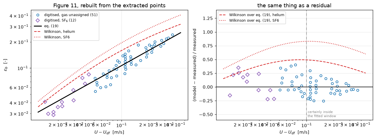
Eq. (19) against all 63 points, gas labels not used: mean absolute deviation 13.8 %, median 11.0 %, worst 40.4 %, bias +2.8 %. The bias is small next to the scatter, so the correlation sits through the points rather than above or below them.
Split at the fitted window. The 33 markers whose excess velocity alone exceeds 0.1 m/s are certainly inside the window Eq. 19 was fitted over: there the mean absolute deviation is 11.1 % and the bias -2.1 %. The other 30 markers include every SF₆ marker, may lie below the window, and are higher: 16.9 % with a bias of +8.3 %. The correlation overpredicts at small excess velocity, which is where a free power law of exponent 0.664 (fitted below to the unlabelled markers) departs from the correlation’s 0.58.
Validation
Four things to check: that the correlation sits through the points it was fitted to, that the scatter is consistent with what the authors report and is not digitisation, how far Wilkinson is from the points, and what the figure can say about gas independence.
d_ours, d_wilk = P["delta_eps_b_this_work"], P["delta_eps_b_wilkinson"]
say(r"""**1. Eq. (19) against the paper's own statistic.** On this figure the mean absolute
deviation is <<mad:.3f>>. The paper's Table 3 gives $\delta = <<d_ours:.3f>>$ for its Eqs. 8 and
19 over its full set. Same order, and this is one column and one liquid, so exact agreement
is neither expected nor a test. The scatter is not digitisation: moving every abscissa by
<<dx:pct1>> and every holdup by <<dy:pct1>> at once, in the direction that raises the predicted
to measured ratio, moves the mean absolute deviation by only <<shift:.2f>> percentage points.

**2. Wilkinson against the same points**, all taken at air density (the mid density,
because the gas labels are not reliable): mean absolute deviation <<w_mad:.3f>>, bias
<<w_bias:+.3f>>. Assuming instead that every point is helium or every point SF₆ gives a
bias of <<w_he:+pct0>> or <<w_sf6:+pct0>>, so the density assumption moves the level but not the
sign: the lowest bias over the four gases is <<w_lo:+pct0>>, and the four differ from each other by
at most <<w_sp:pct0>> points of bias. Table 3 gives $\delta = <<d_wilk:.2f>>$ for Wilkinson. Both say the same thing: Wilkinson
overpredicts, and by a lot. The ratio of mean absolute deviations, Wilkinson to Eq. 19, is
<<ratio:.1f>> here and <<t3:.1f>> in Table 3. This page does not explain the difference. One
candidate is the paper's larger columns, which `F1.3` turns into an implied bias without
testing it here.""",
    mad=M["eq19_mean_abs_dev"], d_ours=d_ours, dx=K["dig_x"], dy=K["dig_y"],
    shift=M["digitisation_shift_mean_abs_dev"] * 100, w_mad=M["wilkinson_mean_abs_dev"],
    w_bias=M["wilkinson_bias"], w_he=M["wilkinson_bias_all_helium"],
    w_sf6=M["wilkinson_bias_all_SF6"], d_wilk=d_wilk,
    w_lo=M["wilkinson_bias_lowest_over_gases"], w_sp=M["wilkinson_bias_spread_over_gases"],
    ratio=M["wilkinson_over_eq19_mean_abs_dev"], t3=M["table3_eps_b_wilkinson_over_replacement"])
1. Eq. (19) against the paper’s own statistic. On this figure the mean absolute deviation is 0.138. The paper’s Table 3 gives \(\delta = 0.160\) for its Eqs. 8 and 19 over its full set. Same order, and this is one column and one liquid, so exact agreement is neither expected nor a test. The scatter is not digitisation: moving every abscissa by 0.5 % and every holdup by 0.4 % at once, in the direction that raises the predicted to measured ratio, moves the mean absolute deviation by only 0.11 percentage points.
2. Wilkinson against the same points, all taken at air density (the mid density, because the gas labels are not reliable): mean absolute deviation 0.639, bias +0.639. Assuming instead that every point is helium or every point SF₆ gives a bias of +47 % or +79 %, so the density assumption moves the level but not the sign: the lowest bias over the four gases is +47 %, and the four differ from each other by at most 33 % points of bias. Table 3 gives \(\delta = 1.25\) for Wilkinson. Both say the same thing: Wilkinson overpredicts, and by a lot. The ratio of mean absolute deviations, Wilkinson to Eq. 19, is 4.6 here and 7.8 in Table 3. This page does not explain the difference. One candidate is the paper’s larger columns, which F1.3 turns into an implied bias without testing it here.
3. The gas-independence claim, and what this figure can say about it
The obvious test, comparing the SF₆ points’ bias against the rest, does not work here, and it is worth saying why rather than quietly reporting the number. On this figure the two groups occupy disjoint velocity windows: every SF₆ point lies at lower excess velocity than every other point, with no overlap at all. A bias difference between them is therefore confounded with velocity. If Eq. 19’s exponent is slightly off at the low end, the SF₆ group will look displaced for a reason that has nothing to do with gas density.
What the data can support is an extrapolation test. Fit a free power law to the unlabelled markers, which are helium, air and argon in an unknown mix, and use it to predict the SF₆ markers, which are denser than any of them and were not seen by the fit. If gas density matters as Wilkinson says it does, SF₆ should sit above that extrapolation (Wilkinson’s rise velocity falls as the gas gets denser), by an amount that depends on which light gas the unlabelled markers are. The standard error of the comparison has two parts: the uncertainty of the extrapolated line (from the fit’s covariance, residual scatter taken from the light markers) and the scatter of the mean of the SF₆ markers about it, assumed independent and log-normal. This statement is measured over extrapolated, not model over measured. This standard error is sampling only: it leaves out the error of continuing a power law below the fitted range, which the figure cannot measure.
light = ~is_sf6
slope, icept = M["light_fit_exponent"], M["light_fit_prefactor"]
say(r"""A free power law fitted on <<n_l:d>> unlabelled markers, <<xlo:.4f>> to <<xhi:.4f>> m/s:
$\varepsilon_b = <<a:.4f>>\,(U-U_{df})^{<<p:.3f>>}$, against Eq. (19) here,
$<<a19:.4f>>\,(U-U_{df})^{<<e19:g>>}$.

Extrapolated onto the <<n_s:d>> SF₆ markers (<<slo:.4f>> to <<shi:.4f>> m/s, $\rho_G$ <<rsf6:g>> against
<<rhe:g>> to <<rar:g>> kg/m³) the model-over-measured deviation has bias <<ext_b:pct1>> in
absolute value (the extrapolation lies below the markers) and mean absolute deviation
<<ext_m:pct1>>, the same scatter as the correlation's own <<mad:pct1>>. The SF₆ markers sit
<<exc:pct1>> above the extrapolation (measured over extrapolated, mean of the point ratios);
in logs the mean excess is <<lex:.3f>>, which is <<geo:pct1>> as a ratio (the geometric mean, not
the mean of the point ratios), with a standard error of <<se:.3f>> in logs, so it is
<<z0:.1f>> standard errors from zero.""",
    n_l=M["n_light"], xlo=x[light].min(), xhi=x[light].max(), a=icept, p=slope,
    a19=K["a19"] * P["column_diameter"] ** K["d19"], e19=K["e19"], n_s=M["n_sf6"],
    slo=x[is_sf6].min(), shi=x[is_sf6].max(), rsf6=GAS["SF6"], rhe=GAS["helium"],
    rar=GAS["argon"], ext_b=M["sf6_extrapolation_bias"], ext_m=M["sf6_extrapolation_mean_abs_dev"],
    mad=M["eq19_mean_abs_dev"], exc=M["sf6_excess_over_extrapolation"],
    lex=M["sf6_log_excess"], geo=M["sf6_excess_geometric"], se=M["sf6_log_excess_se"], z0=M["sf6_excess_z_vs_zero"])
A free power law fitted on 51 unlabelled markers, 0.0508 to 0.3662 m/s: \(\varepsilon_b = 0.4803\,(U-U_{df})^{0.664}\), against Eq. (19) here, \(0.4056\,(U-U_{df})^{0.58}\).
Extrapolated onto the 12 SF₆ markers (0.0143 to 0.0436 m/s, \(\rho_G\) 6.7 against 0.18 to 1.83 kg/m³) the model-over-measured deviation has bias 7.7 % in absolute value (the extrapolation lies below the markers) and mean absolute deviation 13.5 %, the same scatter as the correlation’s own 13.8 %. The SF₆ markers sit 11.7 % above the extrapolation (measured over extrapolated, mean of the point ratios); in logs the mean excess is 0.095, which is 10.0 % as a ratio (the geometric mean, not the mean of the point ratios), with a standard error of 0.080 in logs, so it is 1.2 standard errors from zero.
What Wilkinson requires of the same comparison. Its holdup at the SF₆ markers, relative to the same excess velocity at each candidate light gas, is the number the measured excess has to be compared with. The helium-to-SF₆ spread is the largest, and it is the right comparison only if every unlabelled marker is helium, which the labels do not support.
say(r"""At the SF₆ markers Wilkinson puts the holdup <<w_ar:pct1>> above argon's, <<w_air:pct1>> above
air's and <<w_he:pct1>> above helium's, so for a mix that does not change with velocity, and a
light-gas curve that stays a power law below <<xlo:.3f>> m/s, it requires an excess of
between <<w_ar:pct1>> and <<w_he:pct1>>. The measured excess (<<exc:pct1>>) lies inside that range:
measured minus Wilkinson, in standard errors, is <<z_he:+.1f>> against helium's value and
<<z_ar:+.1f>> against argon's. Eq. (19) requires zero, and the measured excess is <<z0:.1f>>
standard errors from it. **The figure cannot distinguish the two:** the SF₆
markers are consistent with Wilkinson's gas-density dependence, and not inconsistent with
none at all. A mix that changes with velocity, or a curve that bends below the fitted range,
moves what Wilkinson requires by more than the standard error. (At a fixed excess velocity of 0.2 m/s the helium-to-SF₆ spread
Wilkinson predicts is <<gap:pct0>>; no marker of the labelled group sits near that velocity.)""",
    w_ar=M["sf6_wilkinson_excess_over_argon"], w_air=M["sf6_wilkinson_excess_over_air"],
    w_he=M["sf6_wilkinson_excess_over_helium"], exc=M["sf6_excess_over_extrapolation"],
    z_he=M["sf6_excess_z_vs_wilkinson_helium"], z_ar=M["sf6_excess_z_vs_wilkinson_argon"],
    z0=M["sf6_excess_z_vs_zero"], gap=M["wilkinson_predicted_gap_at_0p2"],
    xlo=x[~is_sf6].min())
At the SF₆ markers Wilkinson puts the holdup 5.9 % above argon’s, 7.5 % above air’s and 17.5 % above helium’s, so for a mix that does not change with velocity, and a light-gas curve that stays a power law below 0.051 m/s, it requires an excess of between 5.9 % and 17.5 %. The measured excess (11.7 %) lies inside that range: measured minus Wilkinson, in standard errors, is -0.8 against helium’s value and +0.5 against argon’s. Eq. (19) requires zero, and the measured excess is 1.2 standard errors from it. The figure cannot distinguish the two: the SF₆ markers are consistent with Wilkinson’s gas-density dependence, and not inconsistent with none at all. A mix that changes with velocity, or a curve that bends below the fitted range, moves what Wilkinson requires by more than the standard error. (At a fixed excess velocity of 0.2 m/s the helium-to-SF₆ spread Wilkinson predicts is 25 %; no marker of the labelled group sits near that velocity.)
assert x[is_sf6].max() < K["window"]
say(r"""The SF₆ markers all have excess velocity below <<win:g>> m/s, so none is certainly inside
Eq. 19's fitted window, and a gas-density test on them is a test at small velocity, not at the
churn-turbulent velocities the correlation is for. The paper's own statement, that gas density
does not matter, rests on its full data set and its Figure 6, not on this figure; the page
checks what this figure shows and does not repeat the claim on its behalf.""", win=K["window"])
The SF₆ markers all have excess velocity below 0.1 m/s, so none is certainly inside Eq. 19’s fitted window, and a gas-density test on them is a test at small velocity, not at the churn-turbulent velocities the correlation is for. The paper’s own statement, that gas density does not matter, rests on its full data set and its Figure 6, not on this figure; the page checks what this figure shows and does not repeat the claim on its behalf.
What pymrm adds
Nothing, to the correlation itself, and the honest thing is to say so. This is an algebraic closure; the page calls no pymrm operator, and no pymrm function at all beyond its environment setup. The gallery’s value here is not a better solver but a quantitative test of what the paper states qualitatively, on data extracted from the figure that supports it, and a statement of what that figure cannot show.
What the numbers add is a sharper version of the paper’s case against Wilkinson. Krishna and Ellenberger write that Wilkinson “predicts an exaggerated influence of gas density”. This figure cannot test that: the SF₆ extrapolation is consistent with Wilkinson’s density dependence and with none. What it does show is the level: Wilkinson overpredicts the large-bubble holdup at every gas density, whichever gas the markers are assumed to be, by more than its own density dependence spans.
# Where does Wilkinson's gas-density sensitivity come from? Trace it through.
say(r"""Morton number for tetradecane: $<<mo:tex3>>$.

Wilkinson routes gas density through two exponents, in Eq. 3 and in the excess term of Eq. 4.
The density ratio helium to SF₆ is <<ratio:.1f>>. Raised to the Eq. 3 exponent, $\rho_L/\rho_G$
varies by a factor <<e3:.2f>> from helium to SF₆; raised to the Eq. 4 exponent, by <<e4:.2f>>.
Both are small exponents acting on a large density ratio, and both enter the rise velocity in
the denominator of $\varepsilon_b = (U - U_{\mathrm{trans}})/V_b$, so they survive into the
answer: at an excess velocity of 0.2 m/s Wilkinson's holdup differs by <<gap:pct0>> between
the two gases, against a level error of <<bias:+pct0>> at air.""",
    mo=M["morton_number"], ratio=M["gas_density_ratio_SF6_helium"],
    e3=M["exponent_variation_eq3"], e4=M["exponent_variation_eq4"],
    gap=M["wilkinson_predicted_gap_at_0p2"], bias=M["wilkinson_bias"])

fig, ax = plt.subplots(figsize=(7.0, 4.2))
rho = np.logspace(np.log10(0.1), np.log10(10), 100)
for u, col in zip((0.05, 0.1, 0.2, 0.35), plt.cm.viridis(np.linspace(.15, .85, 4))):
    ax.semilogx(rho, wilkinson(u, rho, K, P) / eq19(u, K, P), color=col, lw=1.8,
                label=f"$U-U_{{df}}$ = {u} m/s")
ax.axhline(1.0, color="k", lw=1.2)
for g, v in GAS.items():
    ax.axvline(v, color="grey", lw=0.8, ls=":")
    ax.text(v, 2.05, g, rotation=90, fontsize=7.5, ha="right", color="grey")
ax.set(xlabel=r"gas density $\rho_G$  [kg/m$^3$]",
       ylabel=r"Wilkinson $\varepsilon_b$ / eq. (19)", ylim=(0.9, 2.2),
       title="the dependence eq. (19) says is not there")
ax.legend(fontsize=8)
fig.tight_layout()
plt.show()
Morton number for tetradecane: \(6.535\times10^{7}\).
Wilkinson routes gas density through two exponents, in Eq. 3 and in the excess term of Eq. 4. The density ratio helium to SF₆ is 37.2. Raised to the Eq. 3 exponent, \(\rho_L/\rho_G\) varies by a factor 1.11 from helium to SF₆; raised to the Eq. 4 exponent, by 1.32. Both are small exponents acting on a large density ratio, and both enter the rise velocity in the denominator of \(\varepsilon_b = (U - U_{\mathrm{trans}})/V_b\), so they survive into the answer: at an excess velocity of 0.2 m/s Wilkinson’s holdup differs by 25 % between the two gases, against a level error of +64 % at air.
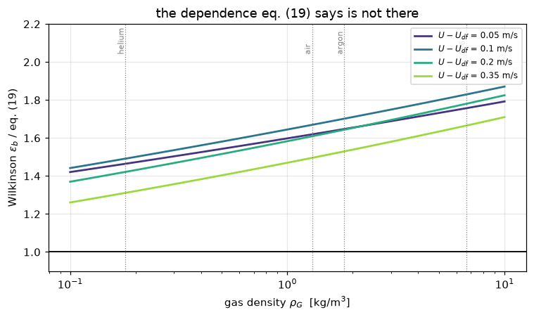
The honest limits of this page. The comparison rests on one figure of the paper’s eleven, so it tests the shape of Eq. 19 in one column and one liquid, and it does not test the column-diameter or liquid-property claims at all (those are Figures 7 and 9; digitising them is the obvious next step). The gas labels exist only for SF₆, which is why the independence test is an extrapolation with a standard error that is comparable to the effect Wilkinson predicts. The scatter of the correlation is the experiment’s: the digitisation error the data sidecar gives accounts for a small fraction of it. And Wilkinson is evaluated at the plotted abscissa rather than from its own transition velocity, which is what the figure caption prescribes but is not the same as running Wilkinson end to end from operating conditions; F1.3 runs it that way.
Reuse
The three correlations are standalone. eq19, wilkinson and reilly_transition take SI arguments, the dictionary of published constants and the parameters, and have no dependence on anything else on this page. eq19 needs only the excess velocity and the column diameter; the other two need the fluid properties, which is exactly the difference at issue.
Where the closure is consumed. A churn-turbulent bubble column model needs \(\varepsilon_b\) to split the gas between a fast large-bubble phase and the dense phase: that is the S7 structure, and F2.3 (Maretto & Krishna’s slurry bubble column for Fischer–Tropsch) is the page that builds it. Use Eq. 19 there in preference to Wilkinson, and use Reilly’s Eq. 8 for the transition, which is what this paper recommends in its conclusions.
Range of validity, from the paper. \(U > 0.1\) m/s and dispersion height above 1 m, the window Eq. 19 was fitted over. Below the regime transition there are no large bubbles to speak of and the correlation has nothing to describe.
Careful with \(U_{df}\). Eq. 19 is written in the measured dense-phase velocity. When predicting rather than correlating you do not have that, and the paper’s recommendation is to substitute Reilly’s \(U_{\mathrm{trans}}\), which is what its own model curves do.
Related pages. F2.3 (the reactor model this feeds), F1.3 (Wilkinson’s correlation end to end, and the abscissa question), F3.1 (gas–liquid reaction regimes), F1.1, F1.6.
Cite the source, not this page: Krishna, R. and Ellenberger, J., Gas holdup in bubble column reactors operating in the churn-turbulent flow regime, AIChE Journal 42(9) 2627–2634 (1996), doi:10.1002/aic.690420923.
# Every number of the page is a claim: a value, held to 1e-6 because the arithmetic is
# closed form (the least-squares fit is a 2x2 solve) and identical under the three BLAS
# kernels, or an exact count decided against a threshold with its margin recorded.
RTOL = 1e-6


def register(M, **special):
    """Register every metric of ``M``: a value claim unless ``special`` gives its
    registration; ``name__margin`` entries are the margins of exact claims."""
    for name, v in M.items():
        if name.endswith("__margin"):
            continue
        if name in special:
            special[name](name, v, M.get(name + "__margin"))
        else:
            claims.value(name, v, rtol=RTOL)


register(M,
         n_points=lambda n, v, m: claims.exact(n, v),
         n_sf6=lambda n, v, m: claims.exact(n, v),
         n_light=lambda n, v, m: claims.exact(n, v),
         n_in_window=lambda n, v, m: claims.exact(n, v, margin=m, min_margin=0.01),
         n_below_window=lambda n, v, m: claims.exact(n, v, margin=m, min_margin=0.01))
The break table
Every number registered above has a row that moves it. Each row mistypes one published constant, or one input of the data (a scaled column, a dropped marker, a changed label, a changed property), and reruns the whole study; the claims it fails are counted. The controls fail nothing.
BREAK = []


def brk(row, metric, broken):
    """One injected defect: ``broken`` is what claim ``metric`` becomes with it."""
    caught = claims.breaks(row, metric, broken)
    BREAK.append((row, metric, claims[metric], broken, caught))
    return caught


def transposed(name, value):
    return f"{PARAM[name]} {K[name]:g} -> {value:g}", {**K, name: value}, C


def with_par(label, name, value):
    return f"{label} {P[name]:g} -> {value:g}", K, replace(C, par={**P, name: value})


def sf6_marker(i):
    return int(np.flatnonzero(C.sf6)[i])


def light_marker(i):
    return int(np.flatnonzero(~C.sf6)[i])


def without(i):
    keep = np.arange(len(C.x)) != i
    return C.x[keep], C.y[keep], C.sf6[keep]


def drop_row(label, i):
    xs_, ys_, fs_ = without(i)
    return f"{label} ({len(C.x)} -> {len(C.x) - 1} points)", K, replace(C, x=xs_, y=ys_, sf6=fs_)


def relabel(i, flag):
    s_ = C.sf6.copy()
    s_[i] = flag
    return f"marker {i} labelled {'SF6' if flag else 'unassigned'} instead of {'unassigned' if flag else 'SF6'}", \
        K, replace(C, sf6=s_)


DEFECTS = [
    transposed("a19", 0.286), transposed("d19", -0.081), transposed("e19", 0.85),
    transposed("window", 0.12),
    transposed("a3", 2.52), transposed("m3", -0.237), transposed("r3", 0.3),
    transposed("a4", 2.0), transposed("e4", 0.577), transposed("m4", 0.077),
    transposed("r4", 0.07),
    transposed("mo_sig", 2), transposed("mo_rho", 2), transposed("mo_g", 1), transposed("mo_mu", -3),
    transposed("g", 9.18),
    transposed("aR", 0.95), transposed("pB", 1.0), transposed("rR", 0.69), transposed("sR", 0.21),
    transposed("vR", 2.48), transposed("vrR", 0.04), transposed("vsR", 0.21),
    transposed("dig_x", 0.05), transposed("dig_y", 0.04),
    with_par("Reilly constant B", "reilly_constant_B", 3.58),
    with_par("column diameter", "column_diameter", 0.19),
    with_par("tetradecane viscosity (mPa s)", "liquid_viscosity", 2.9),
    with_par("surface tension (mN/m)", "surface_tension", 72.0),
    with_par("liquid density", "liquid_density", 673.0),
    with_par("air density", "rho_G_air", 1.2), with_par("helium density", "rho_G_helium", 0.81),
    with_par("argon density", "rho_G_argon", 1.38), with_par("SF6 density", "rho_G_SF6", 7.6),
    with_par("Table 3 Wilkinson eps_b deviation", "delta_eps_b_wilkinson", 1.52),
    with_par("Table 3 replacement eps_b deviation", "delta_eps_b_this_work", 0.61),
    ("abscissa U - U_df scaled by 1.1", K, replace(C, x=C.x * 1.1)),
    ("large-bubble holdup scaled by 1.1", K, replace(C, y=C.y * 1.1)),
    drop_row("an SF6 marker dropped", sf6_marker(0)),
    drop_row("an unlabelled marker dropped", light_marker(0)),
    drop_row("the largest-velocity marker dropped", int(np.argmax(C.x))),
    drop_row("the smallest-velocity marker dropped", int(np.argmin(C.x))),
    relabel(light_marker(0), True), relabel(sf6_marker(0), False),
]
CONTROLS = [
    ("control: clean rerun", K, C),
    ("control: markers in reverse order", K, replace(C, x=C.x[::-1].copy(), y=C.y[::-1].copy(),
                                                     sf6=C.sf6[::-1].copy())),
]
for row, k_, c_ in CONTROLS + DEFECTS:
    for name, value in study(k_, c_).items():
        if not name.endswith("__margin") and name in claims.metrics:
            brk(row, name, value)
# The break table, after every claim is registered: one line per row, with the claims it fails.
by_row = {}
for r_, m_, clean_, broken_, caught_ in BREAK:
by_row.setdefault(r_, []).append((m_, caught_))
controls = [r_ for r_ in by_row if r_.startswith("control")]
_bad = [(r_, m_) for r_, m_, c0, b, c_ in BREAK if c_ and r_ in controls]
assert not _bad, f"a control row failed a claim: {_bad}"
print(f"{'injected defect':<66} {'claims failed':>13} of {'reported':>8}")
for r_, ms in by_row.items():
print(f"{r_[:66]:<66} {sum(c_ for _, c_ in ms):13d} of {len(ms):8d}")
_caught = {m_ for _, m_, _, _, c_ in BREAK if c_}
_open = sorted(k_ for k_ in claims.metrics if k_ not in _caught and not claims.metrics[k_].get("structural"))
print(f"\n{len(by_row)} rows ({len(controls)} controls, which fail no claim); "
f"{len(_caught)} of {len(claims.metrics)} claims are failed by at least one row; "
f"open: {', '.join(_open) or 'none'}")injected defect claims failed of reported
control: clean rerun 0 of 51
control: markers in reverse order 0 of 51
Eq. 19 prefactor 0.268 -> 0.286 10 of 51
Eq. 19 diameter exponent -0.18 -> -0.081 10 of 51
Eq. 19 velocity exponent 0.58 -> 0.85 10 of 51
fitted-window velocity 0.1 -> 0.12 6 of 51
Eq. 3 coefficient 2.25 -> 2.52 15 of 51
Eq. 3 Mo exponent -0.273 -> -0.237 15 of 51
Eq. 3 density exponent 0.03 -> 0.3 16 of 51
Eq. 4 coefficient 2.4 -> 2 15 of 51
Eq. 4 velocity exponent 0.757 -> 0.577 15 of 51
Eq. 4 Mo exponent -0.077 -> 0.077 15 of 51
Eq. 4 density exponent 0.077 -> 0.07 16 of 51
Morton sigma power 3 -> 2 16 of 51
Morton rho_L power 1 -> 2 16 of 51
Morton g power -1 -> 1 16 of 51
Morton mu_L power -4 -> -3 16 of 51
g 9.81 -> 9.18 16 of 51
Eq. 8 coefficient 0.59 -> 0.95 8 of 51
Eq. 8 B exponent 1.5 -> 1 8 of 51
Eq. 8 rho_G exponent 0.96 -> 0.69 8 of 51
Eq. 8 sigma exponent 0.12 -> 0.21 8 of 51
Reilly V_small divisor 2.84 -> 2.48 4 of 51
Reilly V_small rho_G exponent -0.04 -> 0.04 4 of 51
Reilly V_small sigma exponent 0.12 -> 0.21 4 of 51
digitisation error in U - U_df 0.005 -> 0.05 1 of 51
digitisation error in eps_b 0.004 -> 0.04 1 of 51
Reilly constant B 3.85 -> 3.58 8 of 51
column diameter 0.1 -> 0.19 10 of 51
tetradecane viscosity (mPa s) 2.2 -> 2.9 16 of 51
surface tension (mN/m) 27 -> 72 24 of 51
liquid density 763 -> 673 24 of 51
air density 1.3 -> 1.2 7 of 51
helium density 0.18 -> 0.81 11 of 51
argon density 1.83 -> 1.38 5 of 51
SF6 density 6.7 -> 7.6 13 of 51
Table 3 Wilkinson eps_b deviation 1.25 -> 1.52 1 of 51
Table 3 replacement eps_b deviation 0.16 -> 0.61 1 of 51
abscissa U - U_df scaled by 1.1 26 of 51
large-bubble holdup scaled by 1.1 19 of 51
an SF6 marker dropped (63 -> 62 points) 30 of 51
an unlabelled marker dropped (63 -> 62 points) 29 of 51
the largest-velocity marker dropped (63 -> 62 points) 29 of 51
the smallest-velocity marker dropped (63 -> 62 points) 30 of 51
marker 12 labelled SF6 instead of unassigned 16 of 51
marker 0 labelled unassigned instead of SF6 16 of 51
46 rows (2 controls, which fail no claim); 51 of 51 claims are failed by at least one row; open: none# Claims: prints every registered number, writes agreement.json for CI, and
# raises when a claim fails its own check or has no break row.
claims.report(); # the semicolon keeps the notebook from echoing the payloadClaims for F1.4:
n_points = 63 exact exact
n_sf6 = 12 exact exact
n_light = 51 exact exact
n_in_window = 33 exact exact, margin 0.035
n_below_window = 30 exact exact, margin 0.035
eq19_mean_abs_dev = 0.13831 value rtol 1e-06
eq19_median_abs_dev = 0.10981 value rtol 1e-06
eq19_worst_dev = 0.40427 value rtol 1e-06
eq19_bias = 0.028361 value rtol 1e-06
eq19_mean_abs_dev_in_window = 0.11079 value rtol 1e-06
eq19_bias_in_window = -0.021199 value rtol 1e-06
eq19_mean_abs_dev_below_window = 0.16857 value rtol 1e-06
eq19_bias_below_window = 0.082877 value rtol 1e-06
digitisation_shift_mean_abs_dev = 0.0010676 value rtol 1e-06
wilkinson_mean_abs_dev = 0.63942 value rtol 1e-06
wilkinson_bias = 0.63942 value rtol 1e-06
wilkinson_bias_all_helium = 0.46814 value rtol 1e-06
wilkinson_bias_all_air = 0.63942 value rtol 1e-06
wilkinson_bias_all_argon = 0.6707 value rtol 1e-06
wilkinson_bias_all_SF6 = 0.79407 value rtol 1e-06
wilkinson_bias_lowest_over_gases = 0.46814 value rtol 1e-06
wilkinson_bias_spread_over_gases = 0.32594 value rtol 1e-06
wilkinson_over_eq19_mean_abs_dev = 4.6232 value rtol 1e-06
table3_eps_b_wilkinson_over_replacement = 7.8125 value rtol 1e-06
light_fit_exponent = 0.66409 value rtol 1e-06
light_fit_prefactor = 0.4803 value rtol 1e-06
sf6_extrapolation_bias = 0.077235 value rtol 1e-06
sf6_extrapolation_mean_abs_dev = 0.13523 value rtol 1e-06
sf6_excess_over_extrapolation = 0.11684 value rtol 1e-06
sf6_excess_geometric = 0.099725 value rtol 1e-06
sf6_log_excess = 0.09506 value rtol 1e-06
sf6_log_excess_se = 0.0801 value rtol 1e-06
sf6_excess_z_vs_zero = 1.1868 value rtol 1e-06
sf6_wilkinson_excess_over_helium = 0.17478 value rtol 1e-06
sf6_excess_z_vs_wilkinson_helium = -0.8236 value rtol 1e-06
sf6_wilkinson_excess_over_air = 0.074938 value rtol 1e-06
sf6_wilkinson_excess_over_argon = 0.058751 value rtol 1e-06
sf6_excess_z_vs_wilkinson_argon = 0.47412 value rtol 1e-06
wilkinson_predicted_gap_at_0p2 = 0.25251 value rtol 1e-06
morton_number = 6.5352e+07 value rtol 1e-06
gas_density_ratio_SF6_helium = 37.222 value rtol 1e-06
exponent_variation_eq3 = 1.1146 value rtol 1e-06
exponent_variation_eq4 = 1.3211 value rtol 1e-06
reilly_eps_trans_helium = 0.057042 value rtol 1e-06
reilly_U_trans_helium = 0.01315 value rtol 1e-06
reilly_eps_trans_air = 0.14735 value rtol 1e-06
reilly_U_trans_air = 0.02838 value rtol 1e-06
reilly_eps_trans_argon = 0.17364 value rtol 1e-06
reilly_U_trans_argon = 0.031971 value rtol 1e-06
reilly_eps_trans_SF6 = 0.32373 value rtol 1e-06
reilly_U_trans_SF6 = 0.046313 value rtol 1e-06