# Bootstrap: the pymrm this page was checked with, and the gallery files it was
# published with. Works in a checkout, in CI and on a fresh Colab VM.
GALLERY_REF = "gallery-2026.11.10.3"  # replaced by the release tag at publication
PYMRM = ">=3.3.0,<4"  # equals meta.yaml pymrm_min_version, up to the next major
PAGE = "F1.3-wilkinson-high-pressure-holdup"  # equals the page directory

import os, sys, urllib.request
from pathlib import Path
_shared = next((p / "shared" for p in (Path.cwd(), *Path.cwd().parents)
                if (p / "shared" / "gallery_bootstrap.py").is_file()), None)
if _shared is None:
    _shared = (Path(os.environ.get("XDG_CACHE_HOME") or Path.home() / ".cache")
               / "pymrm-gallery" / GALLERY_REF)
    _shared.mkdir(parents=True, exist_ok=True)
    urllib.request.urlretrieve(
        "https://raw.githubusercontent.com/computational-chemical-engineering/"
        f"pymrm-gallery/{GALLERY_REF}/shared/gallery_bootstrap.py",
        _shared / "gallery_bootstrap.py")
sys.path.insert(0, str(_shared))
sys.modules.pop("gallery_bootstrap", None)
from gallery_bootstrap import setup
setup(PAGE, PYMRM, GALLERY_REF); # the semicolon stops the cell echoing the pathWilkinson’s high-pressure bubble-column holdup correlation
sec:F
struct:S1
tier:T1
data:tier4
phase:gas-liquid
Four equations that predict gas holdup from fluid properties alone. Run end to end they say something startling at atmospheric pressure: the homogeneous regime does not exist. That single failure accounts for everything else.
Wilkinson’s high-pressure bubble-column holdup correlation
Catalog ID: F1.3 · Structures: S1 (algebraic closure) · Tier: T1
Wilkinson, Spek and van Dierendonck published a set of four equations that turn fluid properties and a superficial gas velocity into a gas holdup, with no column diameter, no distributor and no fitted constant for the system at hand. It was written for scale-up of high-pressure bubble columns, and pressure enters it in exactly one place: the gas density.
This page runs those four equations end to end and asks where they are well-posed. The answer turns out to be sharp, and it is not the answer the correlation’s reputation would suggest.
# Imports. Packages beyond pymrm and the Colab defaults (numpy, scipy, pandas,
# matplotlib, pyyaml) are installed here with subprocess, not %pip. The
# correlation is algebra; the only pymrm call is pymrm.checks.find_roots, which
# replaces every hand-bracketed root find.
import re
from dataclasses import dataclass, replace

import numpy as np
import pandas as pd
import matplotlib.pyplot as plt
from IPython.display import Markdown, display
from pymrm.checks import find_roots
from gallery_utils import Claims, cite_data, load_claims, load_data, load_meta

plt.rcParams.update({"figure.dpi": 110, "axes.grid": True, "grid.alpha": 0.3})
claims = Claims(PAGE.split("-")[0])
F14 = "F1.4-krishna-ellenberger-holdup"


def fill(text, **v):
    """Fill ``<<name:fmt>>`` in ``text`` from ``v``. Formats are Python formats, or
    ``pctN`` / ``+pctN`` for a fraction shown as a percentage with N decimals, or
    ``texN`` for scientific notation as LaTeX (N decimals)."""
    def sub(m):
        name, _, fmt = m.group(1).partition(":")
        x = v[name]
        mt = re.fullmatch(r"tex(\d+)", fmt)
        if mt:   # a number in scientific notation, as LaTeX
            m_, _, e_ = f"{x:.{mt.group(1)}e}".partition("e")
            return f"{m_}\\times10^{{{int(e_)}}}"
        mp = re.fullmatch(r"(\+?)pct(\d+)", fmt)
        if mp:
            return f"{x * 100:{mp.group(1)}.{mp.group(2)}f} %"
        return format(x, fmt)
    return re.sub(r"<<([^<>]+)>>", sub, text)


def say(text, **v):
    """Prose whose numbers are written by code, so they cannot drift."""
    display(Markdown(fill(text, **v)))
Background
Above roughly 0.1 m/s a bubble column runs churn-turbulent, and the gas splits into two populations: small bubbles that travel with the liquid, and fast large bubbles that short-circuit the column. Design needs the split, because the large bubbles carry most of the throughput and almost none of the residence time.
Wilkinson’s correlation constructs that split from a regime transition. Below a transition velocity \(U_{\mathrm{trans}}\) the column is homogeneous and all gas is small bubbles; above it, the small-bubble holdup freezes at its transition value and every additional cubic metre of gas goes into large bubbles rising at \(V_b\). So the whole correlation pivots on one number, where the transition is, and that number is set by an exponential in the gas density.
A note on the source, because it defines what this page can claim. The original paper, AIChE Journal 38(4) 544–554 (1992), was not available. What is used here is the correlation as reprinted in full by Krishna and Ellenberger (1996), their Eqs. 1–4, verified equation by equation on 600 dpi renders of that paper. Krishna and Ellenberger are testing Wilkinson’s correlation and replacing it, so they are a hostile witness rather than a neutral one; every statement on this page that depends on their opinion is marked as theirs. What does not depend on them is the algebra, which is what most of this page is about. Wilkinson et al. (1992) are cited as the origin of the result; Krishna and Ellenberger (1996) are cited as the text these equations were read from.
What this page is, next to F1.4. F1.4 tests Krishna and Ellenberger’s replacement correlation, Eq. 19, against their Figure 11, and uses Wilkinson only as the foil, evaluating its rise-velocity equations at the plotted abscissa and never touching its transition equation at all. This page runs the correlation as a correlation: Eq. 2 included, from operating conditions, and the transition equation is where everything happens.
The published model
Wilkinson et al. (1992), as printed in Krishna & Ellenberger (1996) Eqs. 1–4. All four were read off a 600 dpi render of journal page 2627.
(1) The split.
\[ \varepsilon_b = \frac{U - U_{\mathrm{trans}}}{V_b}, \qquad \varepsilon = \varepsilon_{\mathrm{small}} + \varepsilon_b . \]
Above the transition the small-bubble holdup is frozen: \(\varepsilon_{\mathrm{small}} = \varepsilon_{\mathrm{trans}}\). That is stated in the running text of page 2628, not in the equations, and again on page 2633 where the total holdup is assembled.
(2) The transition.
\[ U_{\mathrm{trans}} = \varepsilon_{\mathrm{trans}} V_{\mathrm{small}}, \qquad \varepsilon_{\mathrm{trans}} = 0.5\,\exp\!\left(-193\,\rho_G^{-0.61}\mu_L^{0.5}\sigma^{0.11}\right). \]
(3) The small-bubble rise velocity.
\[ \frac{V_{\mathrm{small}}\,\mu_L}{\sigma} = 2.25\left(\frac{\sigma^3\rho_L}{g\mu_L^4}\right)^{-0.273} \left(\frac{\rho_L}{\rho_G}\right)^{0.03}. \]
(4) The large-bubble rise velocity.
\[ \frac{V_b\,\mu_L}{\sigma} = \frac{V_{\mathrm{small}}\,\mu_L}{\sigma} + 2.4\left(\frac{(U-U_{\mathrm{trans}})\mu_L}{\sigma}\right)^{0.757} \left(\frac{\sigma^3\rho_L}{g\mu_L^4}\right)^{-0.077} \left(\frac{\rho_L}{\rho_G}\right)^{0.077}. \]
These four equations are explicit, not coupled. It is worth saying plainly, because the notation suggests otherwise: \(\varepsilon_{\mathrm{trans}}\) does not contain \(U\), so Eq. 2 evaluates first, then Eq. 3, then Eq. 4, then Eq. 1. There is no iteration anywhere and no implicit transition solve. The only place a numerical solve is needed is the inverse problem (given a required \(\varepsilon_b\), find the velocity), and that is well-posed for a separate reason, checked below.
Two things the correlation does not contain. No column diameter, and no distributor. Wilkinson’s is a fluid-property correlation; the column is irrelevant to it. Hold that thought.
The alternative transition closure, printed in the same source as Reilly et al. (1994) Eq. 8, with \(B = 3.85\) from Krishna and Ellenberger’s running text:
\[ \varepsilon_{\mathrm{trans}} = 0.59\,B^{1.5}\sqrt{\frac{\rho_G^{0.96}}{\rho_L}\,\sigma^{0.12}}, \quad V_{\mathrm{small}} = \frac{1}{2.84}\,\rho_G^{-0.04}\sigma^{0.12}, \quad U_{\mathrm{trans}} = V_{\mathrm{small}}\,\varepsilon_{\mathrm{trans}}(1-\varepsilon_{\mathrm{trans}}). \]
Having two closures for the same quantity, printed side by side and applicable to the same systems, is the single most useful thing about this source: it lets each be tested against the other without a figure.
Parameters and assumptions
Assumptions carried into every evaluation below.
- Churn-turbulent operation, \(U > U_{\mathrm{trans}}\). Below the transition Eq. 1 returns a negative \(\varepsilon_b\) and is meaningless; the code clips at zero and the plots start above it.
- Newtonian liquid with a single dynamic viscosity. Eqs. 3 and 4 take one \(\mu_L\), so the paper’s polyacrylamide solutions, for which Table 2 prints four zero-shear viscosities and no single value, are excluded throughout.
- \(\varepsilon_{\mathrm{small}} = \varepsilon_{\mathrm{trans}}\) above the transition, as the source states.
- \(g = 9.81\) m/s², the value the source’s notation list gives.
- Every constant of the four equations, of Reilly’s Eq. 8 and of Eq. 19 lives in one dictionary,
K, that every function takes as an argument. That is what lets the break table at the end of the page mistype one constant at a time and rerun the whole page’s arithmetic.
Sign and direction convention, used everywhere on this page: deviation is always \((\text{model} - \text{measured})/\text{measured}\), so a positive number always means the correlation predicts more holdup than was measured. At large scatter a ratio and its reciprocal are not interchangeable, and F1.4 uses the same convention, so the two pages are directly comparable.
Pressure. Nothing in Eqs. 1–4 is a pressure. Pressure enters only through \(\rho_G\), so a gas substitution at 1 bar and a pressurisation of the same gas are the same experiment as far as this correlation is concerned. That is what makes the four-gas data set below a legitimate pressure surrogate, and it is why the density axis on the last figure carries a second scale in bar.
The data
Four sources, none of them new, and two of them not a dataset at all.
- Marker positions from Figure 11, digitised and maintainer-reviewed for the
F1.4page. Loaded cross-page rather than copied. These are measurements of \(\varepsilon_b\) in a 0.10 m column with tetradecane at four gas densities, and they are the only experimental data on this page. - Table 2’s liquid properties, transcribed here from a 600 dpi render; the Newtonian liquids are usable.
- Table 3’s average relative deviations, already transcribed on the
F1.4page. These are the authors’ statistics over runs whose raw values are not published. They are context, not a target. - Pairs read by eye off Figure 6: \((\rho_G, \varepsilon_{df})\) from panel
- and \((\rho_G, U_{df})\) from panel (b), at the three gas densities that figure labels. The panels carry no (a)/(b) marks and the velocity panel is printed above the voidage one, so the caption is the only authority: “Influence of gas density on the (a) dense-phase gas voidage, and (b) superficial gas velocity through the dense phase”. They are read against the printed axis ticks to two significant figures, with no software digitisation and no coordinates extracted. They are plot markers, not a dataset: no CSV, no sidecar, and none of the transcription checks below uses them.
What F1.4’s page states about the Figure 11 rows, and whether it affects this page. The four series differ only by marker shape, drawn as overlapping open outlines; the maintainer review found the positions trustworthy and the shapes not. Every row except the SF₆ group is therefore unassigned, and no test on this page may depend on series identity. The tests below obey that: the correlation comparison uses positions only, and the one place gas density is needed per point is flagged and handled as a range across the four gases rather than a per-point assignment. F1.4 also computes Wilkinson’s and Eq. 19’s deviations on these same rows; both are printed beside this page’s own below and reconciled. Its abscissa is \(U - U_{df}\) with the measured \(U_{df}\), as the caption states.
obs = load_data("krishna-ellenberger-1996-fig11.csv", page=F14)
par = load_data("krishna-ellenberger-1996-parameters.csv", page=F14)
liq = load_data("krishna-ellenberger-1996-table2-liquids.csv", page=PAGE)
obs_meta = load_meta("krishna-ellenberger-1996-fig11.csv", page=F14)
liq_meta = load_meta("krishna-ellenberger-1996-table2-liquids.csv", page=PAGE)
P = dict(zip(par.quantity, par.value))
F14_CLAIMS = load_claims(F14)

# SI properties for the Newtonian liquids of Table 2: (rho_L, mu_L, sigma)
newt = liq[liq.newtonian == "yes"].copy()
LIQ = {r.liquid: (r.density_kg_m3, r.viscosity_mPa_s * 1e-3, r.surface_tension_mN_m * 1e-3)
       for r in newt.itertuples()}
TETRA = LIQ["Tetradecane"]
WATER = LIQ["Demineralized water"]
is_sf6 = (obs.gas == "SF6").values

# Figure 6, read by eye against the printed axis ticks, two significant figures,
# no software digitisation. Both panels are LINEAR: 0-0.2 for eps_df and
# 0-0.05 m/s for U_df, over rho_G = 0-2 kg/m3, with three labelled markers each.
# The caption reads "Influence of gas density on the (a) dense-phase gas
# voidage, and (b) superficial gas velocity through the dense phase", so eps_df
# is panel (a) and U_df is panel (b). NOT a dataset: no CSV, no sidecar.
FIG6_RHO = np.array([0.18, 1.30, 1.83])          # helium, air, argon
FIG6_EPS_DF = np.array([0.089, 0.139, 0.192])    # Fig. 6(a)
FIG6_U_DF = np.array([0.0161, 0.0230, 0.0269])   # Fig. 6(b)
# Where the authors' own drawn Reilly curves sit in Fig. 6 at rho_G = 0.18 and
# 1.83, read by eye: eps_trans on panel (a), U_trans on panel (b).
FIG6_CURVE_RHO = np.array([0.18, 1.83])
FIG6_CURVE_EPS = np.array([0.055, 0.170])
FIG6_CURVE_U = np.array([0.016, 0.041])


@dataclass(frozen=True)
class Ctx:
    """Everything a study reads that is not a published constant."""
    liquid: tuple          # (rho_L, mu_L, sigma) of the liquid in Figure 11, SI
    liquids: dict          # Newtonian liquids of Table 2, SI
    gas: dict              # gas densities of Figure 11, kg/m3
    x: np.ndarray          # (U - U_df) of the Figure 11 markers, m/s
    y: np.ndarray          # large-bubble holdup of the Figure 11 markers
    fig6_rho: np.ndarray
    fig6_eps: np.ndarray
    fig6_u: np.ndarray
    par: dict              # parameters file: Table 3 deviations, column diameter, B
    xtol: float = 1e-12    # tolerance of every root find, in the variable's unit


C = Ctx(liquid=TETRA, liquids=LIQ,
        gas={"helium": P["rho_G_helium"], "air": P["rho_G_air"],
             "argon": P["rho_G_argon"], "SF6": P["rho_G_SF6"]},
        x=obs.U_minus_Udf.values, y=obs.eps_b.values,
        fig6_rho=FIG6_RHO, fig6_eps=FIG6_EPS_DF, fig6_u=FIG6_U_DF, par=P)
GAS, D_T = C.gas, P["column_diameter"]

print(newt[["liquid", "density_kg_m3", "viscosity_mPa_s", "surface_tension_mN_m"]]
      .to_string(index=False))
print(f"\n{len(liq)} liquids in Table 2, {len(newt)} Newtonian and used")
print(f"{len(obs)} digitised points, {is_sf6.sum()} carrying a gas label; "
      f"(U-U_df) {C.x.min():.4f}-{C.x.max():.4f} m/s, eps_b {C.y.min():.3f}-{C.y.max():.3f}")
print("gas densities, kg/m3: " + ", ".join(f"{k} {v}" for k, v in GAS.items()))
print(f"column {D_T} m, tetradecane; Reilly B = {P['reilly_constant_B']}")
print("\nTable 3, the authors' own average relative deviations (parameters file):")
print(f"   eps_b : Wilkinson eqs. 1-4 {P['delta_eps_b_wilkinson']:.2f}"
      f"   their eqs. 8+19 {P['delta_eps_b_this_work']:.2f}")
print(f"   eps   : Wilkinson eqs. 1-4 {P['delta_eps_total_wilkinson']:.2f}"
      f"   their eqs. 8+19+20 {P['delta_eps_total_this_work']:.2f}")
print("\nFigure 6, read by eye off the printed ticks (markers only, not a dataset):")
for r, e, u in zip(FIG6_RHO, FIG6_EPS_DF, FIG6_U_DF):
    print(f"   rho_G {r:5.2f} kg/m3   eps_df {e:.3f}   U_df {u:.4f} m/s")
print("   the paper's own text: 'increasing gas density significantly increases")
print("   the dense-phase gas voidage (cf. Figure 6)': the direction is printed,")
print("   these three points only put a scale on it.")
print("\nF1.4's own committed deviations on these rows, for reconciliation below:")
for k_ in ("wilkinson_mean_abs_dev", "wilkinson_bias", "eq19_mean_abs_dev", "eq19_bias"):
    print(f"   {k_:24s} {F14_CLAIMS[k_]:.6f}")
print(f"\n{cite_data(obs_meta)}")
print(f"review verdict: {obs_meta['review']['verdict']}")
print(f"{cite_data(liq_meta)}")
liquid density_kg_m3 viscosity_mPa_s surface_tension_mN_m
Demineralized water 998 1.0 72
Tetradecane 763 2.2 27
Paraffin oil (A) 795 2.3 28
Paraffin oil (B) 790 2.9 28
8 liquids in Table 2, 4 Newtonian and used
63 digitised points, 12 carrying a gas label; (U-U_df) 0.0143-0.3662 m/s, eps_b 0.029-0.241
gas densities, kg/m3: helium 0.18, air 1.3, argon 1.83, SF6 6.7
column 0.1 m, tetradecane; Reilly B = 3.85
Table 3, the authors' own average relative deviations (parameters file):
eps_b : Wilkinson eqs. 1-4 1.25 their eqs. 8+19 0.16
eps : Wilkinson eqs. 1-4 0.24 their eqs. 8+19+20 0.23
Figure 6, read by eye off the printed ticks (markers only, not a dataset):
rho_G 0.18 kg/m3 eps_df 0.089 U_df 0.0161 m/s
rho_G 1.30 kg/m3 eps_df 0.139 U_df 0.0230 m/s
rho_G 1.83 kg/m3 eps_df 0.192 U_df 0.0269 m/s
the paper's own text: 'increasing gas density significantly increases
the dense-phase gas voidage (cf. Figure 6)': the direction is printed,
these three points only put a scale on it.
F1.4's own committed deviations on these rows, for reconciliation below:
wilkinson_mean_abs_dev 0.639416
wilkinson_bias 0.639416
eq19_mean_abs_dev 0.138306
eq19_bias 0.028361
Krishna, R.; Ellenberger, J. (1996) — AIChE Journal 42(9) 2627-2634 — doi:10.1002/aic.690420923 — digitised from Figure 11, journal page 2633
review verdict: positions fine, shapes wrong - do not trust the gas labels
Krishna, R.; Ellenberger, J. (1996) — AIChE Journal 42(9) 2627-2634 — doi:10.1002/aic.690420923 — tablePyMRM implementation
This is an algebraic closure, not a discretised model, and dressing it as one would be dishonest. Eqs. 1–4 are four explicit expressions; there is no gradient, no divergence, no Newton solve, and nothing for pymrm’s operators to do. F1.4 says the same about the correlation that replaced it, and the reason is the same: what these correlations are for is to be consumed by a reactor model. The churn-turbulent bubble column with large bubbles in near-plug-flow over a well-mixed dense phase is a genuine S7 coupling, and it is F2.3; \(\varepsilon_b\) is one of its closures.
So what follows is the correlation as five functions, written to be lifted. Every one takes the constants K as an argument. The only pymrm call on the page is pymrm.checks.find_roots, which scans a physically possible range for sign changes and refines each; the page demands exactly one root each time and raises otherwise, so a threshold, a crossing or an inverse solve is never a hand-picked bracket and never a read-off from a grid.
K = dict(  # the published constants, in the order of the equations
    A2=0.5, c2=193.0, p2=-0.61, mu2=0.5, s2=0.11,         # Wilkinson eq. 2
    a3=2.25, m3=-0.273, r3=0.03,                          # eq. 3
    a4=2.4, e4=0.757, m4=-0.077, r4=0.077, v4=1.0,        # eq. 4 (v4: weight of eq. 3's V_small)
    mo_sig=3, mo_rho=1, mo_g=-1, mo_mu=-4,                # exponents of sigma^3 rho_L / (g mu_L^4)
    aR=0.59, B=P["reilly_constant_B"], rR=0.96, sR=0.12,  # Reilly eq. 8, eps_trans
    vR=2.84, vrR=-0.04, vsR=0.12,                         # Reilly eq. 8, V_small
    a19=0.268, d19=-0.18, e19=0.58,                       # Krishna & Ellenberger eq. 19
    D_max=0.63,   # m, the largest column diameter of the runs behind Krishna & Ellenberger's Table 3,
                  # as stated on F1.4 ("six column diameters up to 0.63 m"); not transcribed from the paper here
    g=9.81)
PARAM = {  # what each constant is, for the break-table labels
    "A2": "eq. 2 prefactor", "c2": "eq. 2 constant", "p2": "eq. 2 density exponent",
    "mu2": "eq. 2 viscosity exponent", "s2": "eq. 2 surface-tension exponent",
    "a3": "eq. 3 prefactor", "m3": "eq. 3 Morton exponent", "r3": "eq. 3 density-ratio exponent",
    "a4": "eq. 4 prefactor", "e4": "eq. 4 excess-velocity exponent",
    "m4": "eq. 4 Morton exponent", "r4": "eq. 4 density-ratio exponent",
    "v4": "weight of V_small in eq. 4's first term",
    "mo_sig": "sigma exponent in the Morton group", "mo_rho": "rho_L exponent in the Morton group",
    "mo_g": "g exponent in the Morton group", "mo_mu": "mu_L exponent in the Morton group",
    "aR": "eq. 8 prefactor", "B": "Reilly's B", "rR": "eq. 8 density exponent",
    "sR": "eq. 8 surface-tension exponent", "vR": "eq. 8 V_small divisor",
    "vrR": "eq. 8 V_small density exponent", "vsR": "eq. 8 V_small surface-tension exponent",
    "a19": "eq. 19 prefactor", "d19": "eq. 19 diameter exponent",
    "e19": "eq. 19 excess-velocity exponent", "D_max": "largest column diameter of Table 3's runs", "g": "g"}


def morton(liquid, k=K):
    """The inverse-Morton group sigma^3 rho_L / (g mu_L^4) that Eqs. 3 and 4 use."""
    rho_L, mu_L, sig = liquid
    return (sig ** k["mo_sig"] * rho_L ** k["mo_rho"] * k["g"] ** k["mo_g"]
            * mu_L ** k["mo_mu"])


def wilkinson_transition(rho_G, liquid=TETRA, k=K):
    """Wilkinson et al. (1992) Eqs. 2 and 3. Returns (eps_trans, V_small, U_trans).

    Note that eps_trans does not depend on U: the transition is fixed by the
    fluid properties alone, so this is an evaluation and not a solve.
    """
    rho_L, mu_L, sig = liquid
    rho_G = np.asarray(rho_G, float)
    eps_trans = k["A2"] * np.exp(-k["c2"] * rho_G ** k["p2"] * mu_L ** k["mu2"]
                                 * sig ** k["s2"])
    v_small = (k["a3"] * morton(liquid, k) ** k["m3"] * (rho_L / rho_G) ** k["r3"]
               * sig / mu_L)
    return eps_trans, v_small, eps_trans * v_small


def wilkinson_vb(excess, rho_G, liquid=TETRA, k=K):
    """Wilkinson Eq. 4, the large-bubble rise velocity, at excess = U - U_trans."""
    rho_L, mu_L, sig = liquid
    _, v_small, _ = wilkinson_transition(rho_G, liquid, k)
    ex = np.maximum(np.asarray(excess, float), 0.0)
    second = (k["a4"] * (ex * mu_L / sig) ** k["e4"] * morton(liquid, k) ** k["m4"]
              * (rho_L / np.asarray(rho_G, float)) ** k["r4"] * sig / mu_L)
    return k["v4"] * v_small + second


def wilkinson(U, rho_G, liquid=TETRA, k=K, excess_given=False):
    """The full correlation, Eqs. 1-4, end to end.

    U is the superficial gas velocity; with excess_given=True it is instead
    (U - U_trans) already, which is what Figure 11's model curves plot against.
    Returns a dict of every intermediate, because the intermediates are the
    point of this page.
    """
    eps_trans, v_small, u_trans = wilkinson_transition(rho_G, liquid, k)
    ex = np.asarray(U, float) if excess_given else np.maximum(np.asarray(U, float) - u_trans, 0.0)
    v_b = wilkinson_vb(ex, rho_G, liquid, k)
    eps_b = ex / v_b
    return dict(eps_trans=eps_trans, V_small=v_small, U_trans=u_trans, excess=ex,
                V_b=v_b, eps_b=eps_b, eps=eps_trans + eps_b)


def reilly_transition(rho_G, liquid=TETRA, k=K):
    """Reilly et al. (1994) Eq. 8. Returns (eps_trans, V_small, U_trans)."""
    rho_L, _, sig = liquid
    rho_G = np.asarray(rho_G, float)
    eps = k["aR"] * k["B"] ** 1.5 * np.sqrt(rho_G ** k["rR"] / rho_L * sig ** k["sR"])
    v_small = (1.0 / k["vR"]) * rho_G ** k["vrR"] * sig ** k["vsR"]
    return eps, v_small, v_small * eps * (1.0 - eps)


def eq19(excess, d_t=D_T, k=K):
    """Krishna & Ellenberger Eq. 19, the replacement. No fluid property enters."""
    return k["a19"] * d_t ** k["d19"] * np.asarray(excess, float) ** k["e19"]


def one_root(f, lo, hi, what, xtol=1e-12):
    """The single root of ``f`` on [lo, hi], by pymrm.checks.find_roots. Raises unless
    exactly one sign change is found, so the physical range, not a hand bracket,
    decides, and a second crossing is never silently skipped."""
    out = find_roots(f, lo, hi, log=True, xtol=xtol)
    if len(out["roots"]) != 1:
        raise RuntimeError(f"{what}: expected one root on [{lo:g}, {hi:g}], "
                           f"found {out['message']}")
    return out["roots"][0]


print("Wilkinson eqs. 1-4 evaluated end to end, air-tetradecane, U = 0.20 m/s:")
w = wilkinson(0.20, GAS["air"])
for k_ in ("eps_trans", "V_small", "U_trans", "excess", "V_b", "eps_b", "eps"):
    print(f"   {k_:10s} {float(w[k_]):.6g}")
Wilkinson eqs. 1-4 evaluated end to end, air-tetradecane, U = 0.20 m/s:
eps_trans 0.00280116
V_small 0.245819
U_trans 0.000688579
excess 0.199311
V_b 0.777898
eps_b 0.256218
eps 0.259019Results
Start with the transition, because it is where the correlation is most wrong
Evaluate Eq. 2 for the four gases of Figure 11 and for the four Newtonian liquids of Table 2, alongside Reilly’s Eq. 8 for the same systems. The two closures are answering the identical question, from the identical inputs.
RHO_LO, RHO_HI = 0.1, 1000.0   # gas densities, kg/m3: below helium at 1 bar, up to a liquid-like gas
FIXED_LEVEL = 0.15             # an illustrative fixed eps_trans target, near the measured 0.139 at air
REILLY_LIMIT = 0.32            # the largest eps_trans in Reilly's data, as Krishna & Ellenberger state it
U_OP = 0.20                    # operating velocity of the pressure sweep, m/s
RHO_PLOT = (0.5, 25.0)         # gas densities of the pressure-sweep plot, kg/m3


def transition_study(k, c):
    """Every number of the transition section, for constants ``k`` and context ``c``."""
    L, g_ = c.liquid, c.gas
    eW = lambda r, l=None: float(wilkinson_transition(r, l or L, k)[0])
    eR = lambda r, l=None: float(reilly_transition(r, l or L, k)[0])
    uR = lambda r: float(reilly_transition(r, L, k)[2])
    root = lambda f, lo, hi, what: one_root(f, lo, hi, what, xtol=c.xtol)
    M = {}
    M["eps_trans_wilkinson_air_tetradecane"] = eW(g_["air"])
    M["eps_trans_reilly_air_tetradecane"] = eR(g_["air"])
    M["transition_ratio_reilly_over_wilkinson"] = eR(g_["air"]) / eW(g_["air"])
    M["eps_trans_wilkinson_helium"] = eW(g_["helium"])
    M["U_trans_wilkinson_helium_nm_s"] = float(wilkinson_transition(g_["helium"], L, k)[2]) * 1e9
    M["transition_ratio_helium"] = eR(g_["helium"]) / eW(g_["helium"])
    M["transition_ratio_SF6"] = eR(g_["SF6"]) / eW(g_["SF6"])
    M["eps_trans_reilly_SF6"] = eR(g_["SF6"])
    water = c.liquids["Demineralized water"]
    M["eps_trans_wilkinson_air_water"] = eW(g_["air"], water)
    M["eps_trans_reilly_air_water"] = eR(g_["air"], water)
    M["water_over_tetradecane_wilkinson"] = eW(g_["air"], water) / eW(g_["air"])
    M["tetradecane_over_water_reilly"] = eR(g_["air"]) / eR(g_["air"], water)
    for name, r, e in zip(("helium", "air", "argon"), c.fig6_rho, c.fig6_eps):
        M[f"decades_low_{name}"] = float(np.log10(e / eW(r)))
    # Figure 6, the authors' own drawn Reilly curves against this page's evaluation
    M["reilly_eps_trans_helium_density"] = eR(FIG6_CURVE_RHO[0])
    M["reilly_eps_trans_argon_density"] = eR(FIG6_CURVE_RHO[1])
    M["reilly_U_trans_vs_curve_helium_density"] = uR(FIG6_CURVE_RHO[0]) / FIG6_CURVE_U[0] - 1
    M["reilly_U_trans_vs_curve_argon_density"] = uR(FIG6_CURVE_RHO[1]) / FIG6_CURVE_U[1] - 1
    dev_u = np.array([uR(r) / u - 1 for r, u in zip(c.fig6_rho, c.fig6_u)])
    M["reilly_U_trans_vs_measured_min"], M["reilly_U_trans_vs_measured_max"] = dev_u.min(), dev_u.max()
    # thresholds, crossings and extrema: root-found on the physical range
    r15 = root(lambda r: eW(r) - FIXED_LEVEL, RHO_LO, RHO_HI, "eps_trans(eq. 2) = fixed level")
    r32 = root(lambda r: eR(r) - REILLY_LIMIT, RHO_LO, RHO_HI, "eps_trans(eq. 8) = its data limit")
    r1 = root(lambda r: eR(r) - 1.0, RHO_LO, RHO_HI, "eps_trans(eq. 8) = 1")
    M["rho_G_where_eq2_reaches_0p15"] = r15
    M["rho_G_where_reilly_reaches_0p32"] = r32
    M["rho_G_where_reilly_reaches_1"] = r1
    # U_trans(eq. 8) is stationary where d ln U / d ln rho = 0; multiplying that
    # derivative by (1 - eps) removes the pole at eps = 1
    s_R = 0.5 * k["rR"]
    peak = root(lambda r: k["vrR"] * (1 - eR(r)) + s_R * (1 - 2 * eR(r)), RHO_LO, RHO_HI,
                "stationary point of U_trans(eq. 8)")
    M["rho_G_at_reilly_U_trans_peak"] = peak
    M["reilly_U_trans_peak"] = uR(peak)
    # eq. 8 / eq. 2 is stationary where the two log-slopes are equal
    mu_, sg_ = L[1], L[2]
    slope_W = lambda r: -k["c2"] * k["p2"] * r ** k["p2"] * mu_ ** k["mu2"] * sg_ ** k["s2"]
    rmin = root(lambda r: s_R - slope_W(r), RHO_LO, RHO_HI, "stationary point of eq. 8 / eq. 2")
    M["rho_G_at_eq8_over_eq2_min"] = rmin
    M["eq8_over_eq2_min_ratio"] = eR(rmin) / eW(rmin)
    M["eq8_exceeds_eq2_everywhere"] = bool(eR(rmin) / eW(rmin) > 1.0)
    M["eq8_exceeds_eq2_everywhere__margin"] = eR(rmin) / eW(rmin) - 1.0
    # the measured trend of Figure 6(a), and what it says at the density where eq. 2 reaches the fixed level
    slope, icpt = np.polyfit(np.log(c.fig6_rho), np.log(c.fig6_eps), 1)
    level = float(np.exp(icpt + slope * np.log(r15)))
    M["fig6_eps_df_exponent"] = slope
    M["measured_level_at_rho_0p15"] = level
    M["factor_low_at_rho_0p15"] = level / FIXED_LEVEL
    return M


def sweep_study(k, c):
    """The pressure sweep at U_OP: where the two totals cross, and how eps_b compares with eq. 19."""
    L = c.liquid
    r1 = one_root(lambda r: float(reilly_transition(r, L, k)[0]) - 1.0, RHO_LO, RHO_HI,
                  "eps_trans(eq. 8) = 1", xtol=c.xtol)
    d_t = c.par["column_diameter"]
    M = {}
    def total_gap(r):
        wv = wilkinson(U_OP, r, L, k)
        e2, _, u2 = reilly_transition(r, L, k)
        kb = float(eq19(max(U_OP - float(u2), 1e-9), d_t, k))
        return float(wv["eps"]) - (kb + float(e2) * (1 - kb))
    # on the range where eq. 8 is physical (eps_trans below 1)
    M["rho_G_where_totals_cross"] = one_root(total_gap, RHO_LO, r1, "Wilkinson total = eqs. 8+19+20 total",
                                             xtol=c.xtol)
    # eps_b(eq. 4) / eps_b(eq. 19) at U_OP has one interior maximum in rho_G: the root of the
    # analytic derivative of its logarithm with respect to ln rho_G
    rho_L, mu_L, sig = L
    def ratio_at(r):
        wv = wilkinson(U_OP, r, L, k)
        return float(wv["eps_b"]) / float(eq19(U_OP - float(reilly_transition(r, L, k)[2]), d_t, k))
    def dln_ratio(r):
        e2w, vs, uw = (float(v) for v in wilkinson_transition(r, L, k))
        ex = U_OP - uw
        s_eps = -k["c2"] * k["p2"] * r ** k["p2"] * mu_L ** k["mu2"] * sig ** k["s2"]
        d_uw = uw * (s_eps - k["r3"])                    # d U_trans(eq. 2) / d ln rho_G
        d_ex = -d_uw / ex
        vb = float(wilkinson_vb(ex, r, L, k))
        sec = vb - k["v4"] * vs                          # eq. 4's second term
        d_vb = -k["v4"] * vs * k["r3"] + sec * (k["e4"] * d_ex - k["r4"])
        e2r, _, ur = (float(v) for v in reilly_transition(r, L, k))
        d_ur = ur * (k["vrR"] + 0.5 * k["rR"] * (1 - 2 * e2r) / (1 - e2r))
        return d_ex - d_vb / vb + k["e19"] * d_ur / (U_OP - ur)
    r_peak = one_root(dln_ratio, RHO_LO, r1, "maximum of eps_b(eq. 4) / eps_b(eq. 19)", xtol=c.xtol)
    M["rho_G_at_eps_b_over_eq19_max"] = r_peak
    M["eps_b_wilkinson_over_eq19_max"] = ratio_at(r_peak)
    # the single interior stationary point is a maximum, so the minimum over the plotted range is at one end
    M["eps_b_wilkinson_over_eq19_min"] = min(ratio_at(RHO_PLOT[0]), ratio_at(RHO_PLOT[1]))
    return M


M1 = {**transition_study(K, C), **sweep_study(K, C)}
RHO_AIR = GAS["air"]
rows = []
for gas, rg in GAS.items():
    ew, vw, uw = wilkinson_transition(rg)
    er, vr, ur = reilly_transition(rg)
    rows.append((gas, rg, float(ew), float(uw), float(er), float(ur),
                 float(er / ew), float(ur / uw)))
tab = pd.DataFrame(rows, columns=["gas", "rho_G", "eps_tr_W", "U_tr_W",
                                  "eps_tr_R", "U_tr_R", "ratio_eps", "ratio_U"])
print("gases of Figure 11 in tetradecane, D_T = 0.10 m\n")
print(tab.to_string(index=False, float_format=lambda v: f"{v:12.4g}"))

print("\n\nair in each Newtonian liquid of Table 2\n")
rows = []
for name, props in LIQ.items():
    ew, vw, uw = wilkinson_transition(RHO_AIR, props)
    er, vr, ur = reilly_transition(RHO_AIR, props)
    rows.append((name, props[0], props[1] * 1e3, props[2] * 1e3,
                 float(ew), float(er), float(er / ew)))
print(pd.DataFrame(rows, columns=["liquid", "rho_L", "mu_L/mPa.s", "sigma/mN.m",
                                  "eps_tr_W", "eps_tr_R", "ratio"])
      .to_string(index=False, float_format=lambda v: f"{v:10.4g}"))

print("\nEvery entry in the last column is a factor, not a percentage.")
gases of Figure 11 in tetradecane, D_T = 0.10 m
gas rho_G eps_tr_W U_tr_W eps_tr_R U_tr_R ratio_eps ratio_U
helium 0.18 1.506e-08 3.928e-09 0.05704 0.01315 3.788e+06 3.348e+06
air 1.3 0.002801 0.0006886 0.1474 0.02838 52.6 41.22
argon 1.83 0.007435 0.001809 0.1736 0.03197 23.36 17.67
SF6 6.7 0.07427 0.01738 0.3237 0.04631 4.358 2.664
air in each Newtonian liquid of Table 2
liquid rho_L mu_L/mPa.s sigma/mN.m eps_tr_W eps_tr_R ratio
Demineralized water 998 1 72 0.01019 0.1367 13.42
Tetradecane 763 2.2 27 0.002801 0.1474 52.6
Paraffin oil (A) 795 2.3 28 0.002441 0.1447 59.28
Paraffin oil (B) 790 2.9 28 0.001269 0.1451 114.4
Every entry in the last column is a factor, not a percentage.# Every number of the transition section is a claim: a value, held to 1e-6 because
# the arithmetic is closed form and identical under the three BLAS kernels, or a
# bound, or an exact result decided against a threshold with its margin recorded.
RTOL = 1e-6
def register(M, **special):
"""Register every metric of ``M``: a value claim unless ``special`` gives its
registration; ``name__margin`` entries are the margins of exact claims."""
for name, v in M.items():
if name.endswith("__margin"):
continue
if name in special:
special[name](name, v, M.get(name + "__margin"))
else:
claims.value(name, v, rtol=RTOL)
register(M1, eq8_exceeds_eq2_everywhere=lambda n, v, m: claims.exact(
n, v, margin=m, min_margin=0.1))The two closures are answering the identical question, so the ratio between them is the cleanest statement of how far apart they are.
say(r"""The two closures disagree by a factor of <<SF6:.1f>> at SF₆, <<air:.0f>> at air,
and $<<he:tex1>>$ at helium, where Eq. 2 returns
$\varepsilon_{\mathrm{trans}} = <<e_he:tex1>>$ and a transition velocity of
<<u_he:.1f>> nm/s. Krishna and Ellenberger say Wilkinson's transition
correlation "severely underpredicts" the dense-phase voidage and velocity, and
their Figures 4 and 6 draw both closures against measurement on **logarithmic**
axes spanning three decades, which is the axis you need if one of your two
curves sits at <<e_air:.4f>> and your data sit at <<m_air:.3f>>.""",
    SF6=M1["transition_ratio_SF6"], air=M1["transition_ratio_reilly_over_wilkinson"],
    he=M1["transition_ratio_helium"], e_he=M1["eps_trans_wilkinson_helium"],
    u_he=M1["U_trans_wilkinson_helium_nm_s"], e_air=M1["eps_trans_wilkinson_air_tetradecane"],
    m_air=FIG6_EPS_DF[1])
The two closures disagree by a factor of 4.4 at SF₆, 53 at air, and \(3.8\times10^{6}\) at helium, where Eq. 2 returns \(\varepsilon_{\mathrm{trans}} = 1.5\times10^{-8}\) and a transition velocity of 3.9 nm/s. Krishna and Ellenberger say Wilkinson’s transition correlation “severely underpredicts” the dense-phase voidage and velocity, and their Figures 4 and 6 draw both closures against measurement on logarithmic axes spanning three decades, which is the axis you need if one of your two curves sits at 0.0028 and your data sit at 0.139.
The reason is visible in the functional form. Eq. 2 is \(0.5\exp(-193\,\rho_G^{-0.61}\mu_L^{0.5}\sigma^{0.11})\): at small \(\rho_G\) the argument of the exponential is large and negative, and the whole thing collapses. The prefactor 0.5 is a ceiling approached only as \(\rho_G \to \infty\). So the correlation has a density scale built into it, and the question is where that scale sits.
rho = np.logspace(np.log10(0.1), np.log10(40), 400)
eW, vW, uW = wilkinson_transition(rho)
eR, vR, uR = reilly_transition(rho)

# the measured trend, over the range it was read on and nowhere else
p_eps = np.polyfit(np.log(FIG6_RHO), np.log(FIG6_EPS_DF), 1)
rho_meas = np.logspace(np.log10(FIG6_RHO.min()), np.log10(FIG6_RHO.max()), 40)
rho_ext = np.logspace(np.log10(FIG6_RHO.max()), np.log10(40), 40)
r15, r32 = M1["rho_G_where_eq2_reaches_0p15"], M1["rho_G_where_reilly_reaches_0p32"]

fig, axes = plt.subplots(1, 2, figsize=(11.8, 4.4))
ax = axes[0]
ax.loglog(rho, eW, "-", lw=2, color="tab:red", label="Wilkinson eq. (2)")
ax.loglog(rho, eR, "-", lw=2, color="tab:blue", label="Reilly eq. (8)")
ax.loglog(FIG6_RHO, FIG6_EPS_DF, "ks", ms=6, label=r"measured $\varepsilon_{df}$, Fig. 6(a)")
ax.loglog(rho_meas, np.exp(np.polyval(p_eps, np.log(rho_meas))), "k-", lw=1.0)
ax.loglog(rho_ext, np.exp(np.polyval(p_eps, np.log(rho_ext))), "k:", lw=1.0)
ax.text(2.2, 0.062, f"measured trend $\\propto\\rho_G^{{{p_eps[0]:.2f}}}$;\n"
        "dotted = extrapolated beyond\nthe three points read",
        fontsize=7.0, va="top")
ax.axhline(REILLY_LIMIT, color="tab:blue", ls=":", lw=1.2)
lbl = dict(fontsize=7.5, va="center",
           bbox=dict(facecolor="white", edgecolor="none", pad=1.0))
ax.text(0.115, REILLY_LIMIT, f"Reilly's stated data limit {REILLY_LIMIT}", color="tab:blue", **lbl)
ax.axhline(K["A2"], color="tab:red", ls=":", lw=1.2)
ax.text(0.115, K["A2"], f"Wilkinson's ceiling {K['A2']}", color="tab:red", **lbl)
for g, v in GAS.items():
    ax.axvline(v, color="grey", lw=0.7, ls=":")
    ax.text(v, 3e-8, g, rotation=90, fontsize=7.5, ha="right", va="bottom", color="grey")
ax.set(xlabel=r"gas density $\rho_G$  [kg/m$^3$]", ylabel=r"$\varepsilon_{trans}$  [-]",
       ylim=(1e-8, 1.5), title="the two transition closures")
ax.legend(fontsize=8, loc="lower right")

ax = axes[1]
ax.semilogx(rho, uW, "-", lw=2, color="tab:red", label="Wilkinson eq. (2)")
ax.semilogx(rho, uR, "-", lw=2, color="tab:blue", label="Reilly eq. (8)")
ax.semilogx(FIG6_RHO, FIG6_U_DF, "ks", ms=6, label=r"measured $U_{df}$, Fig. 6(b)")
ax.text(0.115, 0.072, "measured $U_{df}$ rises with density too;\n"
        "the three markers are the only densities read",
        fontsize=7.0, va="top")
ax.set(xlabel=r"gas density $\rho_G$  [kg/m$^3$]",
       ylabel=r"$U_{trans}$  [m/s]", ylim=(0, 0.075),
       title="and the velocity they imply")
ax.legend(fontsize=8, loc="lower right")
fig.tight_layout()
plt.show()

print("how far eq. (2) is below the measurement, at the three densities Fig. 6 gives:")
for (name, r), e in zip(zip(("helium", "air", "argon"), FIG6_RHO), FIG6_EPS_DF):
    ew = float(wilkinson_transition(r)[0])
    print(f"   rho_G {r:5.2f}: measured {e:.3f}, eq. 2 {ew:11.4g}, low by a factor "
          f"{e/ew:11.4g}  ({M1['decades_low_' + name]:.1f} decades)")

print("\ndoes the gap close as the density rises? the two closures never cross:")
print(f"   {'rho_G':>8}{'eq. 2':>10}{'eq. 8':>10}{'eq.8/eq.2':>12}")
for r in (0.18, 1.3, 6.7, 25.0, 70.0, 1000.0):
    print(f"   {r:8.2f}{float(wilkinson_transition(r)[0]):10.4g}"
          f"{float(reilly_transition(r)[0]):10.4g}"
          f"{float(reilly_transition(r)[0])/float(wilkinson_transition(r)[0]):12.4g}")
print(f"   eq. 8 / eq. 2 is stationary at exactly one density, rho_G = "
      f"{M1['rho_G_at_eq8_over_eq2_min']:.1f} kg/m3 (root-found on "
      f"{RHO_LO:g}-{RHO_HI:g}), where it is {M1['eq8_over_eq2_min_ratio']:.2f}.")
print(f"   That is its minimum, since it grows without bound at both ends, so eq. 2 is "
      f"BELOW eq. 8 at every density: {M1['eq8_exceeds_eq2_everywhere']}.")
print(f"\nEq. (2) crosses a FIXED {FIXED_LEVEL} at rho_G = {r15:.1f} kg/m3 "
      f"(~{r15/RHO_AIR:.0f} bar of air).")
print("But the target is not fixed. The paper states that increasing gas density")
print("significantly increases the dense-phase voidage, and the three points read")
print(f"off Fig. 6(a) put that rise at eps_df ~ rho_G^{M1['fig6_eps_df_exponent']:.2f}. "
      f"Extrapolating that")
print(f"three-point fit to {r15:.1f} kg/m3 gives a measured level of "
      f"{M1['measured_level_at_rho_0p15']:.2f}, where eq. 2")
print(f"would still be a factor {M1['factor_low_at_rho_0p15']:.1f} low. So {r15:.0f} kg/m3 "
      "is a LOWER BOUND on where")
print("eq. 2 could become adequate, not the density at which it does, and the")
print("extrapolation is a reconstruction from three read points, not a measurement.")

print(f"\nReilly eq. (8) reaches its own stated data limit {REILLY_LIMIT} at rho_G = {r32:.2f} kg/m3")
print(f"   -> SF6 at {GAS['SF6']} kg/m3 already gives {M1['eps_trans_reilly_SF6']:.3f}, just past it")
print(f"Reilly eq. (8) reaches the impossible eps_trans = 1 at rho_G = "
      f"{M1['rho_G_where_reilly_reaches_1']:.1f} kg/m3")
print(f"and its U_trans is non-monotone: it peaks at {M1['reilly_U_trans_peak']:.4f} m/s at "
      f"rho_G = {M1['rho_G_at_reilly_U_trans_peak']:.1f} kg/m3 and falls")
print("   beyond, because of the (1 - eps_trans) factor, another reason not to")
print("   extrapolate it.")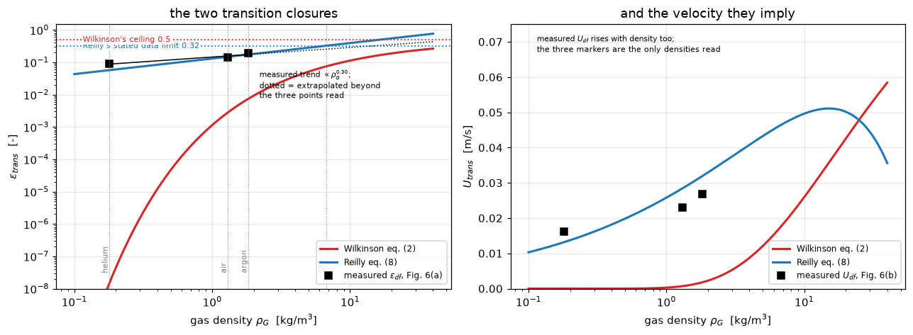
how far eq. (2) is below the measurement, at the three densities Fig. 6 gives:
   rho_G  0.18: measured 0.089, eq. 2   1.506e-08, low by a factor    5.91e+06  (6.8 decades)
   rho_G  1.30: measured 0.139, eq. 2    0.002801, low by a factor       49.62  (1.7 decades)
   rho_G  1.83: measured 0.192, eq. 2    0.007435, low by a factor       25.83  (1.4 decades)

does the gap close as the density rises? the two closures never cross:
      rho_G     eq. 2     eq. 8   eq.8/eq.2
       0.18 1.506e-08   0.05704   3.788e+06
       1.30  0.002801    0.1474        52.6
       6.70   0.07427    0.3237       4.358
      25.00    0.2128    0.6091       2.862
      70.00     0.317    0.9984        3.15
    1000.00     0.457     3.578        7.83
   eq. 8 / eq. 2 is stationary at exactly one density, rho_G = 28.6 kg/m3 (root-found on 0.1-1000), where it is 2.85.
   That is its minimum, since it grows without bound at both ends, so eq. 2 is BELOW eq. 8 at every density: True.

Eq. (2) crosses a FIXED 0.15 at rho_G = 14.2 kg/m3 (~11 bar of air).
But the target is not fixed. The paper states that increasing gas density
significantly increases the dense-phase voidage, and the three points read
off Fig. 6(a) put that rise at eps_df ~ rho_G^0.30. Extrapolating that
three-point fit to 14.2 kg/m3 gives a measured level of 0.32, where eq. 2
would still be a factor 2.1 low. So 14 kg/m3 is a LOWER BOUND on where
eq. 2 could become adequate, not the density at which it does, and the
extrapolation is a reconstruction from three read points, not a measurement.

Reilly eq. (8) reaches its own stated data limit 0.32 at rho_G = 6.54 kg/m3
   -> SF6 at 6.7 kg/m3 already gives 0.324, just past it
Reilly eq. (8) reaches the impossible eps_trans = 1 at rho_G = 70.2 kg/m3
and its U_trans is non-monotone: it peaks at 0.0511 m/s at rho_G = 15.1 kg/m3 and falls
   beyond, because of the (1 - eps_trans) factor, another reason not to
   extrapolate it.
This is the central result of the page, and it is the authors’ own finding made specific. The numbers below are written by code from the cell above.
say(r"""Krishna and Ellenberger write that "the Wilkinson correlation severely underpredicts
the values of the voidage and gas velocity through the dense phase", and they
compare Eq. 2 against their measured $\varepsilon_{df}$ themselves, taking
$\varepsilon_{df} = \varepsilon_{\mathrm{trans}}$. This page runs the same comparison
and puts numbers on "severely": Eq. 2 is **<<d_air:.1f>> decades below the measurement
at air and <<d_ar:.1f>> at argon, and <<d_he:.1f>> decades below it at helium**, where
it returns $\varepsilon_{\mathrm{trans}} = <<e_he:tex1>>$ and a transition velocity of
<<u_he:.1f>> nm/s. The small-bubble population is not merely underpredicted at
helium; it is deleted.

**The gap does not close at higher density.** Two facts, both above:

- Eq. 2 is below Reilly's Eq. 8 at *every* density, not only between
  <<lo:g>> and <<hi:g>> kg/m³: the ratio has a single stationary point, a minimum of
  <<rmin:.2f>> at <<rho_min:.0f>> kg/m³, and rises on both sides, so the two curves
  never cross, visibly so on the left panel. Nothing here shows Wilkinson
  becoming *correct* at any density, only that it stops being absurd.
- The density at which Eq. 2 crosses <<lvl:g>> is not the density at which it
  becomes adequate, because the measured level rises too. Krishna and Ellenberger
  state that outright ("while increasing gas density significantly increases the
  dense-phase gas voidage (cf. Figure 6)") and the three points read off
  Figure 6(a) scale as $\rho_G^{<<p:.2f>>}$. Carried to <<r15:.0f>> kg/m³ that trend
  sits near <<lev:.2f>>, where Eq. 2 would still be a factor of <<fac:.1f>> low.
  **<<r15:.0f>> kg/m³ is a lower bound on where Eq. 2 could become adequate, not a
  crossover**, and the extrapolation behind that sentence is a three-point
  reconstruction rather than a measurement.

**So the two closures are not complementary, and this page does not claim they
are.** They fail in opposite *directions*, which is a different and weaker
statement: Eq. 2 is low everywhere it can be tested and is hard-bounded by its
own prefactor <<A2:g>>, while Reilly's Eq. 8 is the better of the two wherever data
exist but was developed on data reaching only
$\varepsilon_{\mathrm{trans}} = <<lim:g>>$, a ceiling Krishna and Ellenberger state
explicitly, which SF₆ at <<sf6:g>> kg/m³ already passes (it gives <<e_sf6:.3f>>).
Beyond it Eq. 8 turns non-monotone in $U_{\mathrm{trans}}$ at <<pk:.0f>> kg/m³ and
then leaves physics entirely at <<r1:.0f>> kg/m³, where $\varepsilon_{\mathrm{trans}}$
reaches 1. Above <<sf6:g>> kg/m³ **neither** closure has support in this source.

The one thing that is fair to say for Wilkinson is that Krishna and Ellenberger
tested it at <<lo_g:g>> to <<sf6:g>> kg/m³, an order of magnitude below the density
its own title names. That explains where the failure comes from; it does not
repair it.""",
    d_air=M1["decades_low_air"], d_ar=M1["decades_low_argon"], d_he=M1["decades_low_helium"],
    e_he=M1["eps_trans_wilkinson_helium"], u_he=M1["U_trans_wilkinson_helium_nm_s"],
    lo=RHO_LO, hi=RHO_HI, rmin=M1["eq8_over_eq2_min_ratio"], rho_min=M1["rho_G_at_eq8_over_eq2_min"],
    lvl=FIXED_LEVEL, p=M1["fig6_eps_df_exponent"], r15=r15, lev=M1["measured_level_at_rho_0p15"],
    fac=M1["factor_low_at_rho_0p15"], A2=K["A2"], lim=REILLY_LIMIT, sf6=GAS["SF6"],
    e_sf6=M1["eps_trans_reilly_SF6"], pk=M1["rho_G_at_reilly_U_trans_peak"],
    r1=M1["rho_G_where_reilly_reaches_1"], lo_g=GAS["helium"])
Krishna and Ellenberger write that “the Wilkinson correlation severely underpredicts the values of the voidage and gas velocity through the dense phase”, and they compare Eq. 2 against their measured \(\varepsilon_{df}\) themselves, taking \(\varepsilon_{df} = \varepsilon_{\mathrm{trans}}\). This page runs the same comparison and puts numbers on “severely”: Eq. 2 is 1.7 decades below the measurement at air and 1.4 at argon, and 6.8 decades below it at helium, where it returns \(\varepsilon_{\mathrm{trans}} = 1.5\times10^{-8}\) and a transition velocity of 3.9 nm/s. The small-bubble population is not merely underpredicted at helium; it is deleted.
The gap does not close at higher density. Two facts, both above:
- Eq. 2 is below Reilly’s Eq. 8 at every density, not only between 0.1 and 1000 kg/m³: the ratio has a single stationary point, a minimum of 2.85 at 29 kg/m³, and rises on both sides, so the two curves never cross, visibly so on the left panel. Nothing here shows Wilkinson becoming correct at any density, only that it stops being absurd.
- The density at which Eq. 2 crosses 0.15 is not the density at which it becomes adequate, because the measured level rises too. Krishna and Ellenberger state that outright (“while increasing gas density significantly increases the dense-phase gas voidage (cf. Figure 6)”) and the three points read off Figure 6(a) scale as \(\rho_G^{0.30}\). Carried to 14 kg/m³ that trend sits near 0.32, where Eq. 2 would still be a factor of 2.1 low. 14 kg/m³ is a lower bound on where Eq. 2 could become adequate, not a crossover, and the extrapolation behind that sentence is a three-point reconstruction rather than a measurement.
So the two closures are not complementary, and this page does not claim they are. They fail in opposite directions, which is a different and weaker statement: Eq. 2 is low everywhere it can be tested and is hard-bounded by its own prefactor 0.5, while Reilly’s Eq. 8 is the better of the two wherever data exist but was developed on data reaching only \(\varepsilon_{\mathrm{trans}} = 0.32\), a ceiling Krishna and Ellenberger state explicitly, which SF₆ at 6.7 kg/m³ already passes (it gives 0.324). Beyond it Eq. 8 turns non-monotone in \(U_{\mathrm{trans}}\) at 15 kg/m³ and then leaves physics entirely at 70 kg/m³, where \(\varepsilon_{\mathrm{trans}}\) reaches 1. Above 6.7 kg/m³ neither closure has support in this source.
The one thing that is fair to say for Wilkinson is that Krishna and Ellenberger tested it at 0.18 to 6.7 kg/m³, an order of magnitude below the density its own title names. That explains where the failure comes from; it does not repair it.
What that does to the holdup
With \(U_{\mathrm{trans}} \approx 0\) for the lighter gases, Wilkinson’s Eq. 1 assigns essentially all the gas to large bubbles.
U = np.linspace(0.005, 0.45, 300)
fig, axes = plt.subplots(1, 2, figsize=(11.8, 4.4))
cols = dict(zip(GAS, plt.cm.viridis(np.linspace(0.12, 0.85, 4))))

ax = axes[0]
for g, rg in GAS.items():
    w = wilkinson(U, rg)
    ax.plot(U, w["eps_b"], "-", color=cols[g], lw=1.8, label=f"{g}, $\\rho_G$={rg}")
    ax.plot(U, np.full_like(U, float(w["eps_trans"])), ":", color=cols[g], lw=1.3)
ax.set(xlabel="$U$  [m/s]", ylabel=r"holdup  [-]", ylim=(0, 0.42),
       title=r"Wilkinson: $\varepsilon_b$ (solid), $\varepsilon_{small}$ (dotted)")
ax.legend(fontsize=8, loc="upper left")

ax = axes[1]
for g, rg in GAS.items():
    w = wilkinson(U, rg)
    ax.plot(U, w["eps"], "-", color=cols[g], lw=1.8, label=f"{g}")
    er = float(reilly_transition(rg)[0])
    ke = eq19(np.maximum(U - float(reilly_transition(rg)[2]), 0))
    ax.plot(U, ke + er * (1 - ke), "--", color=cols[g], lw=1.3)
ax.set(xlabel="$U$  [m/s]", ylabel=r"total holdup $\varepsilon$  [-]", ylim=(0, 0.55),
       title="total holdup: Wilkinson (solid) vs eqs. 8+19+20 (dashed)")
ax.legend(fontsize=8, loc="upper left")
fig.tight_layout()
plt.show()

print("small-bubble holdup the two routes assign, air-tetradecane:")
print(f"   Wilkinson eq. (2): {M1['eps_trans_wilkinson_air_tetradecane']:.4f}")
print(f"   Reilly    eq. (8): {M1['eps_trans_reilly_air_tetradecane']:.4f}")
print("\nso the dotted lines in the left panel are the entire small-bubble population")
print(f"Wilkinson predicts, and for helium it is {M1['eps_trans_wilkinson_helium']:.1e}: the "
      "homogeneous regime")
print("does not exist at all in this correlation at atmospheric helium density.")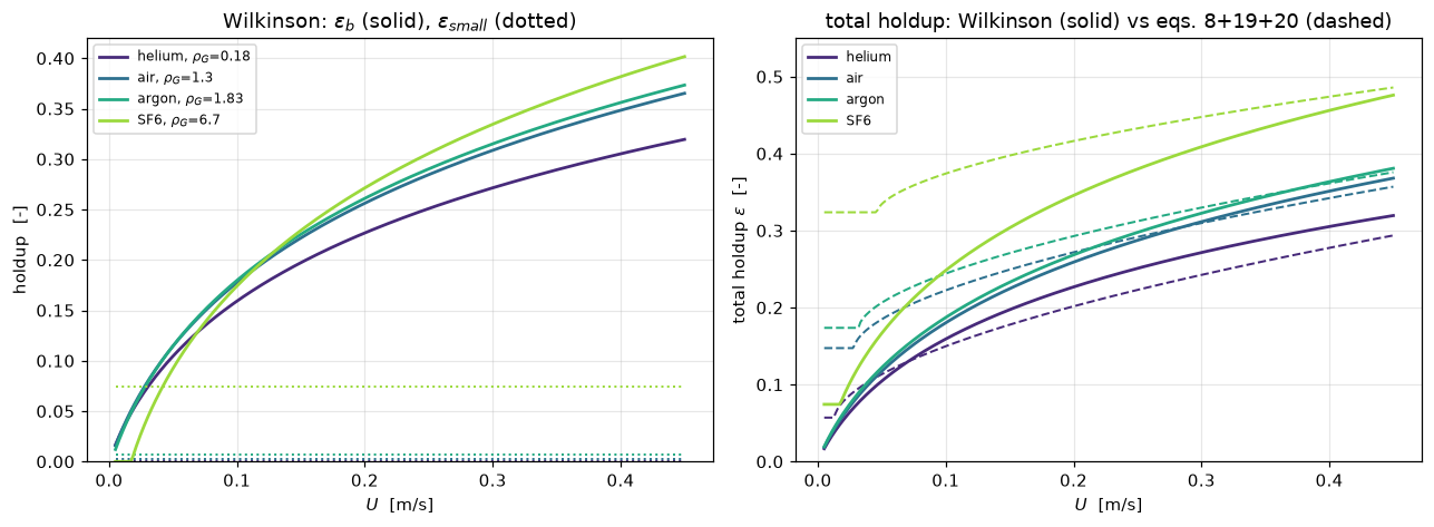
small-bubble holdup the two routes assign, air-tetradecane:
   Wilkinson eq. (2): 0.0028
   Reilly    eq. (8): 0.1474

so the dotted lines in the left panel are the entire small-bubble population
Wilkinson predicts, and for helium it is 1.5e-08: the homogeneous regime
does not exist at all in this correlation at atmospheric helium density.
Validation
Ranked as the gallery ranks them. There is no worked example with printed intermediates in this source, so the strongest routes available are internal identities the correlation must satisfy and the printed statistics, with the Figure 11 markers supplying the only genuine comparison against experiment.
Each check below says what it is: an identity, a reproduction of the authors’ own computed values, or a comparison with measurement. They are not the same thing and the page does not blur them.
1. Dimensional consistency: an identity, and it fails in an informative place
Eqs. 3 and 4 are written as dimensionless groups. Eq. 2 is not written as anything: it is a bare exponential of a dimensional product. Check all of them by exponent arithmetic on (kg, m, s).
Which units the constants are bound to is settled by the source itself, not by inference. Krishna and Ellenberger’s Notation list on their page 2634 prints
\(\sigma\) = surface tension of liquid phase, N·m⁻¹ \(\mu_L\) = liquid viscosity, Pa·s \(\rho_G\) = density of gaseous phase, kg·m⁻³
so Eq. 2 and Eq. 8 are SI-bound by declaration. That matters because both equations are dimensionally inhomogeneous (their constants carry units), so there is no non-dimensional form to fall back on, and feeding them a table of mPa·s is not a scaling error but a catastrophe, as the last lines below show.
DIM = {"rho": np.array([1., -3, 0]), "mu": np.array([1., -1, -1]),
       "sigma": np.array([1., 0, -2]), "g": np.array([0., 1, -2]),
       "velocity": np.array([0., 1, -1])}


def dimension_groups(k):
    """Exponent vectors (kg, m, s) of the groups of Eqs. 3, 4 and of the transition equations."""
    D = DIM
    rise = {
        "Mo = sigma^3 rho_L/(g mu_L^4)": (k["mo_sig"] * D["sigma"] + k["mo_rho"] * D["rho"]
                                         + k["mo_g"] * D["g"] + k["mo_mu"] * D["mu"]),
        "V mu_L/sigma  (eqs. 3, 4 LHS)": D["velocity"] + D["mu"] - D["sigma"],
        "(U-U_tr) mu_L/sigma (eq. 4)": D["velocity"] + D["mu"] - D["sigma"],
        "rho_L/rho_G (eqs. 3, 4)": D["rho"] - D["rho"],
    }
    transition = {
        "eq. 2 exponent argument": k["p2"] * D["rho"] + k["mu2"] * D["mu"] + k["s2"] * D["sigma"],
        "eq. 8 sqrt argument": k["rR"] * D["rho"] - D["rho"] + k["sR"] * D["sigma"],
        "eq. 8 V_small - velocity": k["vrR"] * D["rho"] + k["vsR"] * D["sigma"] - D["velocity"],
    }
    return rise, transition


def identity_study(k, c):
    """The identities and the inverse solves of Validation 1 and 2."""
    L, air = c.liquid, c.gas["air"]
    M = {}
    rise, trans = dimension_groups(k)
    M["dimensionless_groups"] = sum(bool(np.allclose(v, 0, atol=1e-12)) for v in rise.values())
    M["dimensional_transition_groups"] = sum(not np.allclose(v, 0, atol=1e-12) for v in trans.values())
    rho_L, mu_L, sig = L
    M["eq2_value_with_mPa_s_inputs"] = float(wilkinson_transition(air, (rho_L, mu_L * 1e3, sig * 1e3), k)[0])
    _, v_small, u_tr = wilkinson_transition(air, L, k)
    v_small, u_tr = float(v_small), float(u_tr)
    d = np.logspace(-4, -9, 12)
    eb = wilkinson(d, air, L, k, excess_given=True)["eps_b"]
    M["continuity_limit_departure"] = float(abs(1.0 - eb[-1] * v_small / d[-1]))
    # eps_b = ex / V_b has slope (V_small + T2 (1 - e4)) / V_b^2, with T2 the second term of eq. 4
    ex = np.logspace(-9, np.log10(2.0), 4000)
    t2 = wilkinson_vb(ex, air, L, k) - v_small * k["v4"]
    M["eps_b_monotone"] = bool(np.all(k["v4"] * v_small + t2 * (1.0 - k["e4"]) > 0))
    err = 0.0
    for tag, target in (("0p05", 0.05), ("0p15", 0.15), ("0p30", 0.30)):
        f = lambda u, t=target: float(wilkinson(u, air, L, k)["eps_b"]) - t
        us = one_root(f, u_tr, 50.0, f"inverse solve eps_b = {target}", xtol=c.xtol)
        M[f"inverse_U_eps_b_{tag}"] = us
        err = max(err, abs(f(us)))
    M["inverse_roundtrip_error"] = err
    M["U_where_eps_reaches_1"] = one_root(
        lambda u: float(wilkinson(u, air, L, k)["eps"]) - 1.0, 0.1, 1e4, "eps = 1", xtol=c.xtol)
    M["eps_at_U_0p5"] = float(wilkinson(0.5, air, L, k)["eps"])
    return M


M2 = identity_study(K, C)
rise, trans = dimension_groups(K)
print(f"{'group':34s}{'kg':>8}{'m':>8}{'s':>8}   dimensionless?")
for name, v in {**rise, **trans}.items():
    ok = "yes" if np.allclose(v, 0) else "NO"
    print(f"{name:34s}{v[0]:8.3f}{v[1]:8.3f}{v[2]:8.3f}   {ok}")

print(f"\n{M2['dimensionless_groups']} of {len(rise)} groups of Wilkinson's rise-velocity equations "
      "are exactly dimensionless.")
print("Be precise about what that checks: it catches a mis-read exponent INSIDE a")
print("group (sigma^3, mu_L^4, the mu_L/sigma scaling), because those change the")
print("dimensions. It does NOT constrain an exponent applied to an already")
print("dimensionless group (-0.273, -0.077, 0.03, 0.077, 0.757), which stays")
print("dimensionless whatever its value. The transition equations are a different")
print(f"matter again: {M2['dimensional_transition_groups']} of {len(trans)} of their groups are dimensional.")

rho_L, mu_L, sig = TETRA
cgs = float(0.5 * np.exp(-193 * GAS["air"] ** -0.61 * (mu_L * 1e3) ** 0.5 * (sig * 1e3) ** 0.11))
print(f"\neq. 2 with mu_L in Pa s and sigma in N/m  : {M1['eps_trans_wilkinson_air_tetradecane']:.5f}")
print(f"eq. 2 with mu_L in mPa s and sigma in mN/m: {M2['eq2_value_with_mPa_s_inputs']:.3e}")
print("so the constant 193 carries units. The source's own Notation list (p. 2634)")
print("declares sigma in N/m, mu_L in Pa s and rho_G in kg/m3, so SI is the paper's")
print("stated convention, not this page's guess. The mass dimension happens to")
print("cancel in eq. 2 and does not in eq. 8; neither can be non-dimensionalised,")
print("and neither may be fed non-SI inputs, a trap for anyone lifting them out")
print("of a table of mPa s.")
group kg m s dimensionless?
Mo = sigma^3 rho_L/(g mu_L^4) 0.000 0.000 0.000 yes
V mu_L/sigma (eqs. 3, 4 LHS) 0.000 0.000 0.000 yes
(U-U_tr) mu_L/sigma (eq. 4) 0.000 0.000 0.000 yes
rho_L/rho_G (eqs. 3, 4) 0.000 0.000 0.000 yes
eq. 2 exponent argument 0.000 1.330 -0.720 NO
eq. 8 sqrt argument 0.080 0.120 -0.240 NO
eq. 8 V_small - velocity 0.080 -0.880 0.760 NO
4 of 4 groups of Wilkinson's rise-velocity equations are exactly dimensionless.
Be precise about what that checks: it catches a mis-read exponent INSIDE a
group (sigma^3, mu_L^4, the mu_L/sigma scaling), because those change the
dimensions. It does NOT constrain an exponent applied to an already
dimensionless group (-0.273, -0.077, 0.03, 0.077, 0.757), which stays
dimensionless whatever its value. The transition equations are a different
matter again: 3 of 3 of their groups are dimensional.
eq. 2 with mu_L in Pa s and sigma in N/m : 0.00280
eq. 2 with mu_L in mPa s and sigma in mN/m: 2.951e-153
so the constant 193 carries units. The source's own Notation list (p. 2634)
declares sigma in N/m, mu_L in Pa s and rho_G in kg/m3, so SI is the paper's
stated convention, not this page's guess. The mass dimension happens to
cancel in eq. 2 and does not in eq. 8; neither can be non-dimensionalised,
and neither may be fed non-SI inputs, a trap for anyone lifting them out
of a table of mPa s.2. Continuity at the transition: an identity about the correlation’s own structure
As \(U \to U_{\mathrm{trans}}^{+}\), Eq. 4 reduces to \(V_b \to V_{\mathrm{small}}\), so Eq. 1 gives \(\varepsilon_b \to (U-U_{\mathrm{trans}})/V_{\mathrm{small}} \to 0\) and \(\varepsilon \to \varepsilon_{\mathrm{trans}}\). The correlation is therefore continuous across the regime transition, and more than that, its slope \(\mathrm{d}\varepsilon_b/\mathrm{d}U \to 1/V_{\mathrm{small}}\) matches the homogeneous branch \(\varepsilon = U/V_{\mathrm{small}}\) that Eq. 2 implies below the transition, since \(\varepsilon_{\mathrm{trans}} = U_{\mathrm{trans}}/V_{\mathrm{small}}\) is exactly that branch evaluated at \(U_{\mathrm{trans}}\). The correlation is \(C^1\) across its own regime boundary.
That only holds if the first term of Eq. 4 is exactly \(V_{\mathrm{small}}\) from Eq. 3, the same expression and not merely a similar one, so the check below establishes a structural property of the correlation, and that is all it establishes. It is not a check on any exponent. The exponent 0.757 is typed into the function being evaluated, so fitting the rate at which the limit is approached reads it straight back: the genuine external checks on the transcription are the dimensional identity above, including the source’s own declared units, and the reproduction of the authors’ computed lines in §3.
The inverse problem is the only solve the correlation needs. \(\varepsilon_b = (U-U_{\mathrm{trans}})/V_b\) has slope \(\bigl(V_{\mathrm{small}} + T_2(1-0.757)\bigr)/V_b^2 > 0\), with \(T_2\) the second term of Eq. 4, so \(\varepsilon_b\) rises strictly with \(U\) for any exponent below 1 and every inverse is unique; the roots below are found by find_roots on a physical range and the page raises unless there is exactly one.
air = GAS["air"]
_, v_small_air, u_tr_air = wilkinson_transition(air)
v_small_air, u_tr_air = float(v_small_air), float(u_tr_air)
d = np.logspace(-4, -9, 12)
eb = wilkinson(d, air, excess_given=True)["eps_b"]

print(f"V_small(air, tetradecane) = {v_small_air:.5f} m/s,  U_trans = {u_tr_air:.6f} m/s\n")
print(f"{'U - U_trans':>12}{'eps_b':>14}{'(U-U_tr)/V_small':>20}{'1 - ratio':>14}")
for dd, ee in list(zip(d, eb))[::3]:
    print(f"{dd:12.0e}{ee:14.6e}{dd/v_small_air:20.6e}{1-ee*v_small_air/dd:14.4e}")
print("\n  eps_b -> (U - U_trans)/V_small as U -> U_trans, so eps -> eps_trans exactly.")
print(f"  departure from that limit at U - U_trans = {d[-1]:.0e} m/s: "
      f"{M2['continuity_limit_departure']:.2e}")
print("  -> eq. 4's first term is EXACTLY eq. 3's V_small (not merely close to it),")
print("     so the correlation is C1 across its own regime boundary. This is a")
print("     structural identity. It says nothing about whether any exponent was")
print("     transcribed correctly: the exponents are inputs to this arithmetic.")
print(f"\n  d(eps_b)/dU > 0 on U - U_trans from 1e-9 to 2 m/s: {M2['eps_b_monotone']}")
for tag, target in (("0p05", 0.05), ("0p15", 0.15), ("0p30", 0.30)):
    us = M2[f"inverse_U_eps_b_{tag}"]
    back = float(wilkinson(us, air)["eps_b"])
    print(f"  inverse solve: eps_b = {target:.2f} at U = {us:.4f} m/s (round trip {back:.8f})")
print(f"  largest round-trip miss {'below 1e-9'} (here {M2['inverse_roundtrip_error']:.0e})")
print(f"\n  eps reaches 1 only at U = {M2['U_where_eps_reaches_1']:.1f} m/s, far outside any column, so the")
print(f"  correlation stays physical over its whole useful range "
      f"(eps = {M2['eps_at_U_0p5']:.3f} at U = 0.5 m/s).")
V_small(air, tetradecane) = 0.24582 m/s, U_trans = 0.000689 m/s
U - U_trans eps_b (U-U_tr)/V_small 1 - ratio
1e-04 4.040229e-04 4.068027e-04 6.8334e-03
4e-06 1.759828e-05 1.760952e-05 6.3836e-04
2e-07 7.622289e-07 7.622741e-07 5.9298e-05
8e-09 3.299684e-08 3.299703e-08 5.5055e-06
eps_b -> (U - U_trans)/V_small as U -> U_trans, so eps -> eps_trans exactly.
departure from that limit at U - U_trans = 1e-09 m/s: 1.13e-06
-> eq. 4's first term is EXACTLY eq. 3's V_small (not merely close to it),
so the correlation is C1 across its own regime boundary. This is a
structural identity. It says nothing about whether any exponent was
transcribed correctly: the exponents are inputs to this arithmetic.
d(eps_b)/dU > 0 on U - U_trans from 1e-9 to 2 m/s: True
inverse solve: eps_b = 0.05 at U = 0.0170 m/s (round trip 0.05000000)
inverse solve: eps_b = 0.15 at U = 0.0756 m/s (round trip 0.15000000)
inverse solve: eps_b = 0.30 at U = 0.2812 m/s (round trip 0.30000000)
largest round-trip miss below 1e-9 (here 1e-15)
eps reaches 1 only at U = 12.2 m/s, far outside any column, so the
correlation stays physical over its whole useful range (eps = 0.383 at U = 0.5 m/s).register(M2,
dimensionless_groups=lambda n, v, m: claims.exact(n, v),
dimensional_transition_groups=lambda n, v, m: claims.exact(n, v),
eps_b_monotone=lambda n, v, m: claims.exact(
n, v, structural=True,
note="holds for any e4 < 1 and positive constants: slope numerator V_small + T2 (1 - e4)"),
continuity_limit_departure=lambda n, v, m: claims.bound(
n, v, max=1e-5, basis="chosen",
note="the departure at excess 1e-9 m/s is (T2/V_b) with T2 ~ excess^0.757, about 1e-6; "
"a first term other than V_small shifts it by the weight error, orders above 1e-5"),
inverse_roundtrip_error=lambda n, v, m: claims.bound(
n, v, max=1e-9, basis="tolerance",
note="find_roots xtol 1e-12 m/s on U; the slope of eps_b is below 20 per m/s"))4. Against the Figure 11 markers: the only experimental test here
These are measurements, so this is validation. Figure 11’s abscissa is \((U - U_{df})\) with measured \(U_{df}\) for the points, while the model curves on the same axes take \(U_{df} = U_{\mathrm{trans}}\) (the caption says so). Both conventions are evaluated below, because the difference between them is exactly the quantity this page is about, and because F1.4 had to leave it as an open caveat. The comparison is made on every marker and every gas density, not on a hand-picked velocity.
FIXED_U = (0.15, 0.30)   # m/s, the physical velocities of the fixed-velocity table
FIXED_GAS = ("helium", "air", "SF6")


def data_study(k, c):
    """Every number computed from the Figure 11 markers, for constants ``k`` and context ``c``."""
    L, g_, x, y, P_ = c.liquid, c.gas, c.x, c.y, c.par
    d_t = P_["column_diameter"]
    M = {"n_points": len(x), "n_gases": len(g_)}
    rho = g_["air"]
    eb_A = wilkinson(x, rho, L, k, excess_given=True)["eps_b"]
    dev_A = eb_A / y - 1
    M["wilkinson_eps_b_mean_abs_dev"] = float(np.abs(dev_A).mean())
    M["wilkinson_eps_b_bias"] = float(dev_A.mean())
    M["wilkinson_eps_b_worst_dev"] = float(np.abs(dev_A).max())
    M["wilkinson_eps_b_min_dev"] = float(dev_A.min())
    M["wilkinson_dev_gap_to_F1_4"] = abs(float(np.abs(dev_A).mean()) - F14_CLAIMS["wilkinson_mean_abs_dev"])
    dev_19 = eq19(x, d_t, k) / y - 1
    M["eq19_mean_abs_dev"] = float(np.abs(dev_19).mean())
    M["eq19_bias"] = float(dev_19.mean())
    M["eq19_dev_gap_to_F1_4"] = abs(float(np.abs(dev_19).mean()) - F14_CLAIMS["eq19_mean_abs_dev"])
    for gas, rg in g_.items():
        dg = wilkinson(x, rg, L, k, excess_given=True)["eps_b"] / y - 1
        M[f"wilkinson_eps_b_bias_all_{gas}"] = float(dg.mean())
        # eps_b = excess / V_b, so model/measured eps_b is V_b(measured)/V_b(model) at each point;
        # the uniform V_b shortfall that gives the mean bias is 1 - 1/(1 + mean bias)
        M[f"V_b_shortfall_all_{gas}"] = float(1.0 - 1.0 / (1.0 + dg.mean()))
        # a different statistic: the mean over the markers of each marker's own shortfall
        M[f"V_b_shortfall_marker_mean_all_{gas}"] = float(np.mean(1.0 - 1.0 / (1.0 + dg)))
    lo, hi = x.min(), x.max()
    sl_data, _ = np.polyfit(np.log(x), np.log(y), 1)
    sl_w = float((np.log(wilkinson(hi, rho, L, k, excess_given=True)["eps_b"])
                  - np.log(wilkinson(lo, rho, L, k, excess_given=True)["eps_b"]))
                 / (np.log(hi) - np.log(lo)))
    M["wilkinson_secant_slope"], M["measured_free_slope"] = sl_w, float(sl_data)
    M["deviation_corr_with_log_excess"] = float(np.corrcoef(np.log(x), dev_A)[0, 1])
    # the two terms of eq. 4, point by point
    v_small = float(wilkinson_transition(rho, L, k)[1])
    v_b = wilkinson_vb(x, rho, L, k)
    frac = v_small * k["v4"] / v_b
    M["V_small_fraction_of_V_b_mean"] = float(frac.mean())
    M["V_small_fraction_of_V_b_min"], M["V_small_fraction_of_V_b_max"] = float(frac.min()), float(frac.max())
    M["V_small_fraction_at_lowest_excess"] = float(frac[np.argmin(x)])
    second = (v_b - k["v4"] * v_small) / (k["v4"] * v_small)       # T2 / first term
    M["eq4_second_term_larger_points"] = int(np.sum(second > 1.0))
    M["eq4_second_term_larger_points__margin"] = float(np.abs(second - 1.0).min())
    def terms_gap(ex):
        return float(wilkinson_vb(ex, rho, L, k) - 2 * k["v4"] * v_small)
    M["eq4_terms_equal_excess"] = one_root(terms_gap, 1e-4, 10.0, "eq. 4 second term = first term",
                                           xtol=c.xtol)
    # the abscissa convention. Fixed physical velocities first: eps_b with excess U - U_trans(W)
    # against excess U - U_trans(Reilly), as the paper recommends
    ratios = []
    for Uphys in FIXED_U:
        for gas in FIXED_GAS:
            rg = g_[gas]
            utw, udf = float(wilkinson_transition(rg, L, k)[2]), float(reilly_transition(rg, L, k)[2])
            a = float(wilkinson(Uphys - utw, rg, L, k, excess_given=True)["eps_b"])
            b = float(wilkinson(max(Uphys - udf, 1e-9), rg, L, k, excess_given=True)["eps_b"])
            ratios.append(a / b)
    M["abscissa_convention_max_effect"] = float(max(ratios) - 1)
    # then on every marker: physical U = (U - U_df) + U_df, with Reilly's U_trans as the U_df stand-in
    worst = 0.0
    for gas, rg in g_.items():
        udf = float(reilly_transition(rg, L, k)[2])
        e2e = wilkinson(x + udf, rg, L, k)["eps_b"]
        gas_worst = float(np.max(e2e / wilkinson(x, rg, L, k, excess_given=True)["eps_b"] - 1))
        worst = max(worst, gas_worst)
        if gas == "air":
            M["abscissa_effect_max_air_markers"] = gas_worst
        M[f"end_to_end_bias_{gas}"] = float(np.mean(e2e / y - 1))
    M["abscissa_effect_max_all_markers"] = worst
    e2e_meas = wilkinson(x + c.fig6_u[1], c.fig6_rho[1], L, k)["eps_b"]   # air, measured U_df of Fig. 6
    M["end_to_end_bias_air_fig6_U_df"] = float(np.mean(e2e_meas / y - 1))
    # the split of the total holdup
    e_tr_W, e_df_R = float(wilkinson_transition(rho, L, k)[0]), float(reilly_transition(rho, L, k)[0])
    u_df_R = float(reilly_transition(rho, L, k)[2])
    eps_ref = y + e_df_R * (1 - y)                      # eq. 20 with the MEASURED eps_b
    dev_tot = (e_tr_W + eb_A) / eps_ref - 1
    err_small = e_tr_W - e_df_R * (1 - y)
    err_large = eb_A - y
    M["small_bubble_error_mean"], M["large_bubble_error_mean"] = float(err_small.mean()), float(err_large.mean())
    M["total_holdup_error_cancellation"] = float(
        1 - np.abs(err_small + err_large).mean() / (np.abs(err_small).mean() + np.abs(err_large).mean()))
    sel = (x + u_df_R) > 0.1                            # the churn-turbulent window the paper fits
    M["churn_points"] = int(sel.sum())
    M["churn_points__margin"] = float(np.abs(x + u_df_R - 0.1).min() / 0.1)
    M["churn_eps_b_dev"] = float(np.abs(dev_A[sel]).mean())
    M["churn_eps_dev"] = float(np.abs(dev_tot[sel]).mean())
    M["table3_eps_b_wilkinson_over_replacement"] = P_["delta_eps_b_wilkinson"] / P_["delta_eps_b_this_work"]
    M["table3_eps_b_over_eps_wilkinson"] = P_["delta_eps_b_wilkinson"] / P_["delta_eps_total_wilkinson"]
    # the missing diameter term, with eq. 19's own diameter exponent
    M["implied_bias_at_0p63m"] = float((1 + dev_A.mean()) / ((k["D_max"] / d_t) ** k["d19"]) - 1)
    return M


M3 = data_study(K, C)
x_obs, y_obs = C.x, C.y
eb_A = wilkinson(x_obs, GAS["air"], excess_given=True)["eps_b"]
dev_A = eb_A / y_obs - 1
print("deviation is (model - measured)/measured throughout")
print(f"Wilkinson eqs. 1-4, at the plotted abscissa, air density, all {M3['n_points']} points:")
print(f"   mean |dev| {M3['wilkinson_eps_b_mean_abs_dev']*100:5.1f} %   "
      f"bias {M3['wilkinson_eps_b_bias']*100:+5.1f} %   worst {M3['wilkinson_eps_b_worst_dev']*100:5.1f} %")
print(f"   high at every point: the smallest per-point deviation is {M3['wilkinson_eps_b_min_dev']*100:+.1f} %")
print(f"   F1.4 commits {F14_CLAIMS['wilkinson_mean_abs_dev']*100:.1f} % / "
      f"{F14_CLAIMS['wilkinson_bias']*100:+.1f} %; the two pages retype eqs. 3-4 from the same source")
print("   and apply them to the same rows, so that is a transcription cross-check, not an")
print(f"   independent result (gap below 1e-9, here {M3['wilkinson_dev_gap_to_F1_4']:.0e}).")
print(f"   eq. (19) on the same points, for scale: mean |dev| {M3['eq19_mean_abs_dev']*100:.1f} %"
      f"  bias {M3['eq19_bias']*100:+.1f} %   [F1.4 commits "
      f"{F14_CLAIMS['eq19_mean_abs_dev']*100:.1f} % / {F14_CLAIMS['eq19_bias']*100:+.1f} %]")

print("\nthe air-density figure assumes ALL points are air. The gas labels are not")
print("reliable, so the honest statement is the span over the four gases:")
print("   (V_b low by = 1 - 1/(1 + bias), the uniform shortfall that gives the mean bias;")
print("    the marker mean is the mean of each marker's own 1 - 1/(1 + dev), a different statistic)")
for g, rg in GAS.items():
    print(f"   all points as {g:7s} (rho_G {rg:4.2f}): bias {M3['wilkinson_eps_b_bias_all_'+g]*100:+5.1f} %"
          f"   -> V_b low by {M3['V_b_shortfall_all_'+g]*100:4.1f} %"
          f"   (marker mean {M3['V_b_shortfall_marker_mean_all_'+g]*100:4.1f} %)")
bias_all = [M3[f"wilkinson_eps_b_bias_all_{g}"] for g in GAS]
span = max(bias_all) - min(bias_all)
short_all = [M3[f"V_b_shortfall_all_{g}"] for g in GAS]
print(f"   so the bias is {min(bias_all)*100:+.0f} to {max(bias_all)*100:+.0f} %, a span of "
      f"{span*100:.0f} pp (about +-{span*50:.0f} pp about the mid-span),")
print(f"   and the implied V_b shortfall is {min(short_all)*100:.0f}-{max(short_all)*100:.0f} %. "
      "Every attribution below carries that.")

print(f"\npower-law slope over {x_obs.min():.4f}-{x_obs.max():.4f} m/s:")
print(f"   measured (free fit, all {M3['n_points']})  {M3['measured_free_slope']:.3f}")
print(f"   Wilkinson secant             {M3['wilkinson_secant_slope']:.3f}")
print(f"   eq. (19) by construction     {K['e19']:.3f}")
print(f"   correlation of Wilkinson's deviation with log(U-U_df): "
      f"{M3['deviation_corr_with_log_excess']:+.3f}")
print("   -> over this window Wilkinson's error is mostly a LEVEL error, not a slope error:")
print("      the shape it predicts is if anything closer to the data than eq. 19's,")
print("      and it is the magnitude that is wrong.")

print("\nThe split of V_b between its two terms, air density, point by point:")
print(f"   V_small supplies {M3['V_small_fraction_of_V_b_mean']*100:.0f} % of V_b on average "
      f"(range {M3['V_small_fraction_of_V_b_min']*100:.0f}-{M3['V_small_fraction_of_V_b_max']*100:.0f} %, "
      f"{M3['V_small_fraction_at_lowest_excess']*100:.0f} % at the lowest excess velocity).")
print(f"   The two terms are equal at U - U_trans = {M3['eq4_terms_equal_excess']:.4f} m/s "
      f"(root-found); the second term is the larger one at "
      f"{M3['eq4_second_term_larger_points']} of the {M3['n_points']} points,")
print("   so eq. 4's own second term dominates most of this data, and eq. 3's V_small the")
print("   lowest-velocity third. The error belongs to the rise-velocity pair, not to eq. 4")
print("   with eq. 3 exonerated.")

print("\nThe abscissa convention. First at fixed physical velocities, with Reilly's U_trans as")
print("the stand-in for the measured U_df, which is what the paper recommends. Note how")
print("good that stand-in actually is, against the three U_df values read off Fig. 6:")
for r, um in zip(FIG6_RHO, FIG6_U_DF):
    ur_ = float(reilly_transition(r)[2])
    print(f"   rho_G {r:5.2f}: measured {um:.4f}, Reilly {ur_:.4f} m/s  ({(ur_/um-1)*100:+5.0f} %)")
print(f"   -> Reilly's U_trans is itself {M1['reilly_U_trans_vs_measured_min']*100:+.0f} to "
      f"{M1['reilly_U_trans_vs_measured_max']*100:+.0f} % against the measurement.")
print(f"   {'U':>6}{'gas':>9}{'U_tr(W)':>10}{'U_df(R)':>10}{'eps_b(W)':>10}{'eps_b(R)':>10}{'ratio':>8}")
for Uphys in FIXED_U:
    for g in FIXED_GAS:
        rg = GAS[g]
        utw = float(wilkinson_transition(rg)[2])
        udf = float(reilly_transition(rg)[2])
        a = float(wilkinson(Uphys - utw, rg, excess_given=True)["eps_b"])
        b = float(wilkinson(max(Uphys - udf, 1e-9), rg, excess_given=True)["eps_b"])
        print(f"   {Uphys:6.2f}{g:>9}{utw:10.5f}{udf:10.4f}{a:10.4f}{b:10.4f}{a/b:8.3f}")
print(f"   At these {len(FIXED_U) * len(FIXED_GAS)} conditions the convention is worth at most "
      f"{M3['abscissa_convention_max_effect']*100:.0f} % in eps_b, because the excess velocity is large.")
print(f"\nBut the markers are not at large excess. On every one of the {M3['n_points']} markers and "
      "every gas, running end to end")
print(f"from the physical velocity (U - U_df) + U_df instead of at the plotted abscissa raises eps_b by up to "
      f"{M3['abscissa_effect_max_all_markers']*100:.0f} %,")
print("most at the lowest excess velocities, where the transition velocity Wilkinson does not")
print("predict is a large fraction of the whole. The mean bias becomes:")
print(f"   {'gas':>8}{'at the abscissa':>18}{'end to end':>14}")
for g in GAS:
    print(f"   {g:>8}{M3['wilkinson_eps_b_bias_all_'+g]*100:+17.0f} %{M3['end_to_end_bias_'+g]*100:+13.0f} %")
print(f"   with the measured U_df of Fig. 6 instead of Reilly's (air): "
      f"{M3['end_to_end_bias_air_fig6_U_df']*100:+.0f} %")
print("So F1.4's caveat is NOT closed: the convention does not matter at large excess, and")
print("matters a great deal at small excess, which is where eq. 2's failure acts. The two")
print("defects are separable, and they compound; neither hides inside the other.")
print("\nSo the eps_b overprediction and the transition failure are TWO defects,")
print("not one, and they can be separated here:")
print("   at the measured excess velocity, eq. 2 does not enter at all, so the")
print(f"   {M3['wilkinson_eps_b_bias']*100:+.0f} % belongs to eqs. 3 and 4 JOINTLY, and running end to end adds eq. 2's")
print("   transition error on top of it. Two things bound the attribution: the gas-density")
print(f"   span above, and the fact that this figure is one {D_T} m column while Wilkinson carries")
print("   no diameter term, so part of the rise-velocity share may be a missing diameter")
print("   effect rather than a wrong rise velocity, see (b) below.")
deviation is (model - measured)/measured throughout
Wilkinson eqs. 1-4, at the plotted abscissa, air density, all 63 points:
mean |dev| 63.9 % bias +63.9 % worst 133.5 %
high at every point: the smallest per-point deviation is +9.9 %
F1.4 commits 63.9 % / +63.9 %; the two pages retype eqs. 3-4 from the same source
and apply them to the same rows, so that is a transcription cross-check, not an
independent result (gap below 1e-9, here 0e+00).
eq. (19) on the same points, for scale: mean |dev| 13.8 % bias +2.8 % [F1.4 commits 13.8 % / +2.8 %]
the air-density figure assumes ALL points are air. The gas labels are not
reliable, so the honest statement is the span over the four gases:
(V_b low by = 1 - 1/(1 + bias), the uniform shortfall that gives the mean bias;
the marker mean is the mean of each marker's own 1 - 1/(1 + dev), a different statistic)
all points as helium (rho_G 0.18): bias +46.8 % -> V_b low by 31.9 % (marker mean 30.0 %)
all points as air (rho_G 1.30): bias +63.9 % -> V_b low by 39.0 % (marker mean 37.4 %)
all points as argon (rho_G 1.83): bias +67.1 % -> V_b low by 40.1 % (marker mean 38.6 %)
all points as SF6 (rho_G 6.70): bias +79.4 % -> V_b low by 44.3 % (marker mean 42.8 %)
so the bias is +47 to +79 %, a span of 33 pp (about +-16 pp about the mid-span),
and the implied V_b shortfall is 32-44 %. Every attribution below carries that.
power-law slope over 0.0143-0.3662 m/s:
measured (free fit, all 63) 0.636
Wilkinson secant 0.621
eq. (19) by construction 0.580
correlation of Wilkinson's deviation with log(U-U_df): -0.109
-> over this window Wilkinson's error is mostly a LEVEL error, not a slope error:
the shape it predicts is if anything closer to the data than eq. 19's,
and it is the magnitude that is wrong.
The split of V_b between its two terms, air density, point by point:
V_small supplies 46 % of V_b on average (range 23-77 %, 77 % at the lowest excess velocity).
The two terms are equal at U - U_trans = 0.0719 m/s (root-found); the second term is the larger one at 42 of the 63 points,
so eq. 4's own second term dominates most of this data, and eq. 3's V_small the
lowest-velocity third. The error belongs to the rise-velocity pair, not to eq. 4
with eq. 3 exonerated.
The abscissa convention. First at fixed physical velocities, with Reilly's U_trans as
the stand-in for the measured U_df, which is what the paper recommends. Note how
good that stand-in actually is, against the three U_df values read off Fig. 6:
rho_G 0.18: measured 0.0161, Reilly 0.0131 m/s ( -18 %)
rho_G 1.30: measured 0.0230, Reilly 0.0284 m/s ( +23 %)
rho_G 1.83: measured 0.0269, Reilly 0.0320 m/s ( +19 %)
-> Reilly's U_trans is itself -18 to +23 % against the measurement.
U gas U_tr(W) U_df(R) eps_b(W) eps_b(R) ratio
0.15 helium 0.00000 0.0131 0.1972 0.1883 1.048
0.15 air 0.00069 0.0284 0.2217 0.1988 1.116
0.15 SF6 0.01738 0.0463 0.2292 0.1994 1.150
0.30 helium 0.00000 0.0131 0.2714 0.2663 1.019
0.30 air 0.00069 0.0284 0.3087 0.2958 1.044
0.30 SF6 0.01738 0.0463 0.3345 0.3183 1.051
At these 6 conditions the convention is worth at most 15 % in eps_b, because the excess velocity is large.
But the markers are not at large excess. On every one of the 63 markers and every gas, running end to end
from the physical velocity (U - U_df) + U_df instead of at the plotted abscissa raises eps_b by up to 138 %,
most at the lowest excess velocities, where the transition velocity Wilkinson does not
predict is a large fraction of the whole. The mean bias becomes:
gas at the abscissa end to end
helium +47 % +66 %
air +64 % +106 %
argon +67 % +114 %
SF6 +79 % +128 %
with the measured U_df of Fig. 6 instead of Reilly's (air): +99 %
So F1.4's caveat is NOT closed: the convention does not matter at large excess, and
matters a great deal at small excess, which is where eq. 2's failure acts. The two
defects are separable, and they compound; neither hides inside the other.
So the eps_b overprediction and the transition failure are TWO defects,
not one, and they can be separated here:
at the measured excess velocity, eq. 2 does not enter at all, so the
+64 % belongs to eqs. 3 and 4 JOINTLY, and running end to end adds eq. 2's
transition error on top of it. Two things bound the attribution: the gas-density
span above, and the fact that this figure is one 0.1 m column while Wilkinson carries
no diameter term, so part of the rise-velocity share may be a missing diameter
effect rather than a wrong rise velocity, see (b) below.5. Why Table 3 says what it says
The authors report two pairs of numbers over the runs of Table 3: for the large-bubble holdup, Wilkinson against their own correlation; for the total holdup, the same two, which come out essentially level. Their \(\delta\) is printed as \(\frac{1}{N}\sum |{\rm exp}_i - {\rm pred}_i| / {\rm exp}_i\), which is the same quantity as the mean \(|(\text{model}-\text{measured})/\text{measured}|\) used on this page, so the magnitudes are directly comparable even though the runs are not.
Those raw values are not published, so none of this reproduces Table 3. What can be done is to show that its pattern follows necessarily from what has already been computed, using the markers that are available.
Two things have to be accounted for: why Wilkinson is several times worse than its replacement on \(\varepsilon_b\) and level with it on \(\varepsilon\), and why the Table 3 value for \(\varepsilon_b\) is about twice what is found here on one column.
print("(a) the two errors have opposite signs and largely cancel")
print("    NOTE the small-bubble term uses REILLY's eps_df as the stand-in for the")
print("    measured small-bubble holdup, because no measured small-bubble holdup is")
print("    published for these runs. That term is therefore a model, not data.")
es, el = M3["small_bubble_error_mean"], M3["large_bubble_error_mean"]
print(f"    small-bubble term  mean {es:+.4f}")
print(f"    large-bubble term  mean {el:+.4f}")
print(f"    the cancellation, 1 - |net| / (|small| + |large|) on the point-wise errors: "
      f"{M3['total_holdup_error_cancellation']*100:.0f} %")
print("    That percentage is close to a restatement: for two opposite-signed terms")
print("    it is just 2*min/(|a|+|b|), i.e. another way of writing the ratio of the")
print("    two terms above. Nothing is fitted to Table 3 (its values are not inputs to")
print("    any of this), but the cancellation figure carries no more information than")
print("    the two terms it is built from.")
print(f"\n    relative deviation, the {M3['churn_points']} points with implied U > 0.1 m/s:")
print(f"       eps_b {M3['churn_eps_b_dev']:.3f}   eps {M3['churn_eps_dev']:.3f}   "
      f"ratio {M3['churn_eps_b_dev']/M3['churn_eps_dev']:.1f}x")
print(f"    printed Table 3: eps_b {P['delta_eps_b_wilkinson']:.2f} vs eps "
      f"{P['delta_eps_total_wilkinson']:.2f}, a ratio of {M3['table3_eps_b_over_eps_wilkinson']:.1f}x;")
print(f"    against its replacement on eps_b ({P['delta_eps_b_this_work']:.2f}) Wilkinson is "
      f"{M3['table3_eps_b_wilkinson_over_replacement']:.1f} times worse")
print("    Same structure, and it is not a coincidence: the authors note that")
print("    Wilkinson was fitted to total gas holdup, never to the split, so the")
print("    split is where an error can hide, and hide it partly does. The two")
print(f"    errors are NOT equal and opposite: eq. 2 underpredicts eps_small by "
      f"{abs(es):.3f},")
print(f"    about {abs(es)/abs(el):.1f} times the {abs(el):.3f} by which eq. 1 overpredicts eps_b, "
      "so the")
print("    total is left with the difference rather than with nothing.")
print("    CAVEAT: eps_ref above uses the measured eps_b plus Reilly's eps_df, not")
print("    a measured total holdup, so the eps column is indicative. The printed")
print("    Table 3 totals are the measurement-based statement, and they are the authors'.")

# (b) the missing column-diameter term
print("\n(b) Wilkinson has no diameter term; eq. 19 says the diameter matters")
print(f"    measured here at D_T = {D_T} m: Wilkinson biased {M3['wilkinson_eps_b_bias']*100:+.0f} %")
print(f"    {'D_T/m':>8}{'eq.19 factor':>15}{'implied Wilkinson bias':>26}")
for dt in (D_T, K["D_max"]):
    f = (dt / D_T) ** K["d19"]
    print(f"    {dt:8.3f}{f:15.3f}{((1 + M3['wilkinson_eps_b_bias']) / f - 1)*100:+25.0f} %")
print("    0.63 m is the largest column of Table 3's runs, as F1.4 records. Table 3's runs span")
print(f"    several diameters and give {P['delta_eps_b_wilkinson']:.2f}; the range implied here is "
      f"{M3['wilkinson_eps_b_bias']:.2f} to {M3['implied_bias_at_0p63m']:.2f}.")
print("    This is an internal-consistency argument between two of the paper's own results")
print("    (eq. 19's diameter exponent and Table 3's statistic), not a reproduction of either.")
(a) the two errors have opposite signs and largely cancel
NOTE the small-bubble term uses REILLY's eps_df as the stand-in for the
measured small-bubble holdup, because no measured small-bubble holdup is
published for these runs. That term is therefore a model, not data.
small-bubble term mean -0.1279
large-bubble term mean +0.0662
the cancellation, 1 - |net| / (|small| + |large|) on the point-wise errors: 68 %
That percentage is close to a restatement: for two opposite-signed terms
it is just 2*min/(|a|+|b|), i.e. another way of writing the ratio of the
two terms above. Nothing is fitted to Table 3 (its values are not inputs to
any of this), but the cancellation figure carries no more information than
the two terms it is built from.
relative deviation, the 42 points with implied U > 0.1 m/s:
eps_b 0.617 eps 0.171 ratio 3.6x
printed Table 3: eps_b 1.25 vs eps 0.24, a ratio of 5.2x;
against its replacement on eps_b (0.16) Wilkinson is 7.8 times worse
Same structure, and it is not a coincidence: the authors note that
Wilkinson was fitted to total gas holdup, never to the split, so the
split is where an error can hide, and hide it partly does. The two
errors are NOT equal and opposite: eq. 2 underpredicts eps_small by 0.128,
about 1.9 times the 0.066 by which eq. 1 overpredicts eps_b, so the
total is left with the difference rather than with nothing.
CAVEAT: eps_ref above uses the measured eps_b plus Reilly's eps_df, not
a measured total holdup, so the eps column is indicative. The printed
Table 3 totals are the measurement-based statement, and they are the authors'.
(b) Wilkinson has no diameter term; eq. 19 says the diameter matters
measured here at D_T = 0.1 m: Wilkinson biased +64 %
D_T/m eq.19 factor implied Wilkinson bias
0.100 1.000 +64 %
0.630 0.718 +128 %
0.63 m is the largest column of Table 3's runs, as F1.4 records. Table 3's runs span
several diameters and give 1.25; the range implied here is 0.64 to 1.28.
This is an internal-consistency argument between two of the paper's own results
(eq. 19's diameter exponent and Table 3's statistic), not a reproduction of either.register(M3,
n_points=lambda n, v, m: claims.exact(n, v),
n_gases=lambda n, v, m: claims.exact(n, v),
wilkinson_dev_gap_to_F1_4=lambda n, v, m: claims.bound(
n, v, max=1e-9, basis="chosen",
note="the same arithmetic on the same rows as F1.4's committed value, so equal to "
"round-off; 1e-9 is far above round-off and far below any transcription change"),
eq19_dev_gap_to_F1_4=lambda n, v, m: claims.bound(
n, v, max=1e-9, basis="chosen",
note="as wilkinson_dev_gap_to_F1_4, for eq. 19"),
eq4_second_term_larger_points=lambda n, v, m: claims.exact(n, v, margin=m, min_margin=0.01),
churn_points=lambda n, v, m: claims.exact(n, v, margin=m, min_margin=0.005))The break table
Every number registered above has a row that moves it. Each row mistypes one published constant (two digits transposed, a sign flipped, a wrong round) or one input, then reruns the arithmetic of the whole page and reports what every claim becomes. The labels are built from the values the rows inject. Two control rows change nothing that matters (a clean rerun, the markers in reverse order) and must fail no claim.
BREAK = []   # (injected defect, claim, clean value, broken value, caught)
REFUSED = []  # (injected defect, study, reason) where the page's own one-root demand stopped a study
current_row = [""]


def brk(row, metric, broken):
    """One injected defect: ``broken`` is what claim ``metric`` becomes with it."""
    caught = claims.breaks(row, metric, broken)
    BREAK.append((row, metric, claims[metric], broken, caught))
    return caught


def run_all(k, c):
    """The arithmetic of the whole page for constants ``k`` and context ``c``."""
    out = {}
    for study in (transition_study, sweep_study, identity_study, data_study):
        try:
            part = study(k, c)
        except RuntimeError as err:   # a defect the page itself refuses is reported, not counted
            REFUSED.append((current_row[0], study.__name__, str(err)))
            continue
        assert not set(part) & set(out), "two studies report the same claim"
        out.update(part)
    return out


def transposed(name, value):
    return f"{PARAM[name]} {K[name]:g} -> {value:g}", {**K, name: value}, C


def eq8_dimensionless():
    """Reilly's eq. 8 density and surface-tension exponents changed so that its sqrt argument is dimensionless."""
    return (f"{PARAM['rR']} {K['rR']:g} -> 1 and {PARAM['sR']} {K['sR']:g} -> 0", {**K, "rR": 1.0, "sR": 0.0}, C)


def with_gas(name, value):
    return (f"{name} density {C.gas[name]:g} -> {value:g} kg/m3", K,
            replace(C, gas={**C.gas, name: value}))


def with_fig6(field, i, value):
    arr = getattr(C, field).copy()
    old = arr[i]
    arr[i] = value
    return f"Figure 6 {field.split('_', 1)[1]} read at rho_G {C.fig6_rho[i]:g}: {old:g} -> {value:g}", K, replace(C, **{field: arr})


L_slow = (TETRA[0], 2.9e-3, TETRA[2])
DEFECTS = [
    transposed("A2", 0.6), transposed("c2", 139.0), transposed("p2", -0.51),
    transposed("mu2", 0.6), transposed("s2", 0.17),
    transposed("a3", 2.52), transposed("m3", -0.237), transposed("r3", 0.3),
    transposed("a4", 2.0), transposed("e4", 0.577), transposed("m4", 0.077),
    transposed("r4", 0.07), transposed("v4", 0.9),
    transposed("mo_sig", 2), transposed("mo_rho", 2), transposed("mo_g", 1), transposed("mo_mu", -3),
    transposed("aR", 0.95), transposed("B", 3.58), transposed("B", 1.9), transposed("rR", 0.69), transposed("sR", 0.21),
    transposed("vR", 2.48), transposed("vrR", 0.04), transposed("vsR", 0.21),
    transposed("a19", 0.286), transposed("d19", -0.081), transposed("e19", 0.85),
    transposed("g", 9.18),
    eq8_dimensionless(),
    with_gas("air", 1.2), with_gas("SF6", 7.6),
    (f"a fifth gas added, nitrogen at 1.14 kg/m3 ({len(C.gas)} -> {len(C.gas) + 1} gases)", K,
     replace(C, gas={**C.gas, "nitrogen": 1.14})),
    (f"tetradecane viscosity {TETRA[1]*1e3:g} -> {L_slow[1]*1e3:g} mPa s (paraffin oil B)", K, replace(C, liquid=L_slow)),
    (f"abscissa U - U_df scaled by {1.1:g}", K, replace(C, x=C.x * 1.1)),
    (f"large-bubble holdup scaled by {1.1:g}", K, replace(C, y=C.y * 1.1)),
    (f"last marker dropped ({len(C.x)} -> {len(C.x) - 1} points)", K, replace(C, x=C.x[:-1], y=C.y[:-1])),
    with_fig6("fig6_eps", 1, 0.193), with_fig6("fig6_u", 1, 0.0320),
    (f"Table 3 Wilkinson eps_b deviation {P['delta_eps_b_wilkinson']:g} -> 1.52", K,
     replace(C, par={**P, "delta_eps_b_wilkinson": 1.52})),
    (f"column diameter {D_T:g} -> 0.19 m", K, replace(C, par={**P, "column_diameter": 0.19})),
    (f"root tolerance {C.xtol:g} -> 0.001", K, replace(C, xtol=1e-3)),
]
CONTROLS = [
    ("control: clean rerun", K, C),
    ("control: markers in reverse order", K, replace(C, x=C.x[::-1].copy(), y=C.y[::-1].copy())),
]
for row, k_, c_ in CONTROLS + DEFECTS:
    current_row[0] = row
    for name, value in run_all(k_, c_).items():
        if not name.endswith("__margin") and name in claims.metrics:
            brk(row, name, value)
# The break table, after every claim is registered: one line per row, with the claims it fails.
by_row = {}
for r_, m_, clean_, broken_, caught_ in BREAK:
by_row.setdefault(r_, []).append((m_, caught_))
controls = [r_ for r_ in by_row if r_.startswith("control")]
_bad = [(r_, m_) for r_, m_, c0, b, c_ in BREAK if c_ and r_ in controls]
assert not _bad, f"a control row failed a claim: {_bad}"
print(f"{'injected defect':<84} {'claims failed':>13} of {'reported':>8}")
for r_, ms in by_row.items():
print(f"{r_[:84]:<84} {sum(c_ for _, c_ in ms):13d} of {len(ms):8d}")
for r_, st_, why in REFUSED:
print(f"refused by the page itself, {st_} not rerun: {r_}")
_caught = {m_ for _, m_, _, _, c_ in BREAK if c_}
_open = sorted(k_ for k_ in claims.metrics if k_ not in _caught and not claims.metrics[k_].get("structural"))
print(f"\n{len(by_row)} rows ({len(controls)} controls, which fail no claim); "
f"{len(_caught)} of {len(claims.metrics)} claims are failed by at least one row; "
f"open: {', '.join(_open) or 'none'}")injected defect claims failed of reported
control: clean rerun 0 of 95
control: markers in reverse order 0 of 95
eq. 2 prefactor 0.5 -> 0.6 34 of 95
eq. 2 constant 193 -> 139 37 of 95
eq. 2 density exponent -0.61 -> -0.51 37 of 95
eq. 2 viscosity exponent 0.5 -> 0.6 37 of 95
eq. 2 surface-tension exponent 0.11 -> 0.17 37 of 95
eq. 3 prefactor 2.25 -> 2.52 48 of 95
eq. 3 Morton exponent -0.273 -> -0.237 44 of 91
eq. 3 density-ratio exponent 0.03 -> 0.3 44 of 91
eq. 4 prefactor 2.4 -> 2 47 of 95
eq. 4 excess-velocity exponent 0.757 -> 0.577 44 of 91
eq. 4 Morton exponent -0.077 -> 0.077 38 of 80
eq. 4 density-ratio exponent 0.077 -> 0.07 47 of 95
weight of V_small in eq. 4's first term 1 -> 0.9 48 of 95
sigma exponent in the Morton group 3 -> 2 49 of 95
rho_L exponent in the Morton group 1 -> 2 45 of 91
g exponent in the Morton group -1 -> 1 49 of 95
mu_L exponent in the Morton group -4 -> -3 45 of 91
eq. 8 prefactor 0.59 -> 0.95 33 of 95
Reilly's B 3.85 -> 3.58 33 of 95
Reilly's B 3.85 -> 1.9 34 of 95
eq. 8 density exponent 0.96 -> 0.69 28 of 91
eq. 8 surface-tension exponent 0.12 -> 0.21 34 of 95
eq. 8 V_small divisor 2.84 -> 2.48 19 of 95
eq. 8 V_small density exponent -0.04 -> 0.04 17 of 95
eq. 8 V_small surface-tension exponent 0.12 -> 0.21 19 of 95
eq. 19 prefactor 0.268 -> 0.286 6 of 95
eq. 19 diameter exponent -0.18 -> -0.081 7 of 95
eq. 19 excess-velocity exponent 0.58 -> 0.85 7 of 95
g 9.81 -> 9.18 47 of 95
eq. 8 density exponent 0.96 -> 1 and eq. 8 surface-tension exponent 0.12 -> 0 36 of 95
air density 1.3 -> 1.2 kg/m3 35 of 95
SF6 density 6.7 -> 7.6 kg/m3 7 of 95
a fifth gas added, nitrogen at 1.14 kg/m3 (4 -> 5 gases) 1 of 95
tetradecane viscosity 2.2 -> 2.9 mPa s (paraffin oil B) 63 of 95
abscissa U - U_df scaled by 1.1 40 of 95
large-bubble holdup scaled by 1.1 31 of 95
last marker dropped (63 -> 62 points) 37 of 95
Figure 6 eps read at rho_G 1.3: 0.139 -> 0.193 4 of 95
Figure 6 u read at rho_G 1.3: 0.023 -> 0.032 2 of 95
Table 3 Wilkinson eps_b deviation 1.25 -> 1.52 2 of 95
column diameter 0.1 -> 0.19 m 7 of 95
root tolerance 1e-12 -> 0.001 7 of 95
refused by the page itself, sweep_study not rerun: eq. 3 Morton exponent -0.273 -> -0.237
refused by the page itself, sweep_study not rerun: eq. 3 density-ratio exponent 0.03 -> 0.3
refused by the page itself, sweep_study not rerun: eq. 4 excess-velocity exponent 0.757 -> 0.577
refused by the page itself, sweep_study not rerun: eq. 4 Morton exponent -0.077 -> 0.077
refused by the page itself, identity_study not rerun: eq. 4 Morton exponent -0.077 -> 0.077
refused by the page itself, sweep_study not rerun: rho_L exponent in the Morton group 1 -> 2
refused by the page itself, sweep_study not rerun: mu_L exponent in the Morton group -4 -> -3
refused by the page itself, sweep_study not rerun: eq. 8 density exponent 0.96 -> 0.69
44 rows (2 controls, which fail no claim); 94 of 95 claims are failed by at least one row; open: noneWhat pymrm adds
Nothing to the correlation itself, and the honest thing is to say so. Eqs. 1–4 are algebra; no pymrm operator appears on this page. The one pymrm call is pymrm.checks.find_roots, used for every threshold, crossing, extremum and inverse solve: it scans the physically possible range for sign changes, refines each, and this page raises unless it finds exactly one. That replaces hand-picked brackets and grid read-offs, and it is a check as well as a solver: a second root, or none, would stop the page. The gallery’s contribution here is otherwise not a solver but a dissection, and several of its results are not in the source.
say(r"""**First, the correlation has two defects, and they can be separated.**
Krishna and Ellenberger report that Wilkinson underpredicts the dense-phase
parameters and overpredicts the large-bubble holdup, and give a statistic for
each. Running the equations end to end shows these are *not* the same fact.
Eq. 2 puts the regime transition <<d_ar:.1f>>–<<d_air:.1f>> decades too low at argon and air
and <<d_he:.1f>> decades too low at helium, which empties the small-bubble population;
that defect is entirely Eq. 2's, and at <<sf6:g>> kg/m³ it is still a factor of
<<r_sf6:.1f>> against Reilly while at <<he_rho:g>> kg/m³ it is a factor of $<<r_he:tex1>>$.
But at the *measured* excess velocity Eq. 2 does not enter at all, and the
<<bias:+pct0>> on $\varepsilon_b$ belongs instead to **Eqs. 3 and 4 jointly**: $V_b$ is
<<short:pct0>> low on average over the points, and $V_b$'s first term *is* Eq. 3's
$V_{\mathrm{small}}$, which supplies <<fr:pct0>> of $V_b$ on average (<<fr_lo:pct0>> to
<<fr_hi:pct0>>, and <<fr_first:pct0>> at the lowest excess velocity). The second term of
Eq. 4 is the larger of the two at <<n2:d>> of the <<n:d>> points, above an excess
of <<ex:.3f>> m/s. What is *not* wrong is the shape: over the window Figure 11
covers, the power-law slope Wilkinson predicts (<<sw:.3f>>) is closer to the measured
<<sm:.3f>> than the replacement correlation's <<se:.2f>> is. The error is in the level,
in two places, for two reasons.

**The air-density figure carries a stated uncertainty**, because the gas labels on
Figure 11 are not reliable and every point is therefore evaluated at air density.
Redoing it at the other gases gives <<b_he:+pct0>> (helium) to <<b_sf6:+pct0>> (SF₆),
a <<span:.0f>> pp span, and a $V_b$ shortfall of <<s_lo:pct0>> to <<s_hi:pct0>> rather than a
single <<short:pct0>>. The decomposition survives that span; the third significant figure
does not.

**Second, the two transition closures fail in opposite directions; they are not
complementary.** Reilly's Eq. 8 exceeds Wilkinson's Eq. 2 at every gas density; the
ratio bottoms out at <<rmin:.2f>> near <<rho_min:.0f>> kg/m³ and rises again, so the curves
never cross and there is no density above which Wilkinson takes over. Eq. 2 is low
wherever it can be tested and is hard-bounded by its own prefactor <<A2:g>>, while Eq. 8
is the better of the two where data exist but passes its authors' stated ceiling of
<<lim:g>> just past SF₆ at <<sf6:g>> kg/m³, turns non-monotone in $U_{\mathrm{trans}}$ at
<<pk:.0f>> kg/m³ and exceeds 1 at <<r1:.0f>>. **Above <<sf6:g>> kg/m³ neither closure has
support in this source**, and that, not a division of labour, is what a reader
choosing between them needs to know.

**Third, the abscissa question `F1.4` had to leave open is answered, and the answer
is that it matters.** At the fixed physical velocities of the table above the
convention is worth at most <<fixed:pct0>> in $\varepsilon_b$, but on the markers
themselves, which sit at small excess velocity, it is worth up to <<allm:pct0>>. Running
the correlation end to end from a physical velocity, with Reilly's $U_{\mathrm{trans}}$
standing in for the measured $U_{\mathrm{df}}$, the mean bias on $\varepsilon_b$ is
<<e2e_air:+pct0>> at air against <<bias:+pct0>> at the plotted abscissa
(<<e2e_fig6:+pct0>> with the $U_{\mathrm{df}}$ read off Figure 6). The two defects compound.

The pressure extrapolation below is the natural use of a correlation whose only
pressure dependence is $\rho_G$, and it is an extrapolation, with nothing here to
test it against.""",
    d_ar=M1["decades_low_argon"], d_air=M1["decades_low_air"], d_he=M1["decades_low_helium"],
    sf6=GAS["SF6"], r_sf6=M1["transition_ratio_SF6"], he_rho=GAS["helium"], r_he=M1["transition_ratio_helium"],
    bias=M3["wilkinson_eps_b_bias"], short=M3["V_b_shortfall_all_air"],
    fr=M3["V_small_fraction_of_V_b_mean"], fr_lo=M3["V_small_fraction_of_V_b_min"],
    fr_hi=M3["V_small_fraction_of_V_b_max"], fr_first=M3["V_small_fraction_at_lowest_excess"],
    n2=M3["eq4_second_term_larger_points"], n=M3["n_points"], ex=M3["eq4_terms_equal_excess"],
    sw=M3["wilkinson_secant_slope"], sm=M3["measured_free_slope"], se=K["e19"],
    b_he=M3["wilkinson_eps_b_bias_all_helium"], b_sf6=M3["wilkinson_eps_b_bias_all_SF6"],
    span=span * 100, s_lo=min(short_all), s_hi=max(short_all),
    rmin=M1["eq8_over_eq2_min_ratio"], rho_min=M1["rho_G_at_eq8_over_eq2_min"], A2=K["A2"],
    lim=REILLY_LIMIT, pk=M1["rho_G_at_reilly_U_trans_peak"], r1=M1["rho_G_where_reilly_reaches_1"],
    fixed=M3["abscissa_convention_max_effect"], allm=M3["abscissa_effect_max_all_markers"],
    e2e_air=M3["end_to_end_bias_air"], e2e_fig6=M3["end_to_end_bias_air_fig6_U_df"])
First, the correlation has two defects, and they can be separated. Krishna and Ellenberger report that Wilkinson underpredicts the dense-phase parameters and overpredicts the large-bubble holdup, and give a statistic for each. Running the equations end to end shows these are not the same fact. Eq. 2 puts the regime transition 1.4–1.7 decades too low at argon and air and 6.8 decades too low at helium, which empties the small-bubble population; that defect is entirely Eq. 2’s, and at 6.7 kg/m³ it is still a factor of 4.4 against Reilly while at 0.18 kg/m³ it is a factor of \(3.8\times10^{6}\). But at the measured excess velocity Eq. 2 does not enter at all, and the +64 % on \(\varepsilon_b\) belongs instead to Eqs. 3 and 4 jointly: \(V_b\) is 39 % low on average over the points, and \(V_b\)’s first term is Eq. 3’s \(V_{\mathrm{small}}\), which supplies 46 % of \(V_b\) on average (23 % to 77 %, and 77 % at the lowest excess velocity). The second term of Eq. 4 is the larger of the two at 42 of the 63 points, above an excess of 0.072 m/s. What is not wrong is the shape: over the window Figure 11 covers, the power-law slope Wilkinson predicts (0.621) is closer to the measured 0.636 than the replacement correlation’s 0.58 is. The error is in the level, in two places, for two reasons.
The air-density figure carries a stated uncertainty, because the gas labels on Figure 11 are not reliable and every point is therefore evaluated at air density. Redoing it at the other gases gives +47 % (helium) to +79 % (SF₆), a 33 pp span, and a \(V_b\) shortfall of 32 % to 44 % rather than a single 39 %. The decomposition survives that span; the third significant figure does not.
Second, the two transition closures fail in opposite directions; they are not complementary. Reilly’s Eq. 8 exceeds Wilkinson’s Eq. 2 at every gas density; the ratio bottoms out at 2.85 near 29 kg/m³ and rises again, so the curves never cross and there is no density above which Wilkinson takes over. Eq. 2 is low wherever it can be tested and is hard-bounded by its own prefactor 0.5, while Eq. 8 is the better of the two where data exist but passes its authors’ stated ceiling of 0.32 just past SF₆ at 6.7 kg/m³, turns non-monotone in \(U_{\mathrm{trans}}\) at 15 kg/m³ and exceeds 1 at 70. Above 6.7 kg/m³ neither closure has support in this source, and that, not a division of labour, is what a reader choosing between them needs to know.
Third, the abscissa question F1.4 had to leave open is answered, and the answer is that it matters. At the fixed physical velocities of the table above the convention is worth at most 15 % in \(\varepsilon_b\), but on the markers themselves, which sit at small excess velocity, it is worth up to 138 %. Running the correlation end to end from a physical velocity, with Reilly’s \(U_{\mathrm{trans}}\) standing in for the measured \(U_{\mathrm{df}}\), the mean bias on \(\varepsilon_b\) is +106 % at air against +64 % at the plotted abscissa (+99 % with the \(U_{\mathrm{df}}\) read off Figure 6). The two defects compound.
The pressure extrapolation below is the natural use of a correlation whose only pressure dependence is \(\rho_G\), and it is an extrapolation, with nothing here to test it against.
U_op = U_OP
rho = np.logspace(np.log10(RHO_PLOT[0]), np.log10(RHO_PLOT[1]), 300)
P_bar = rho / GAS["air"]   # air at fixed T, rho_G linear in P, anchored on the air density = 1 bar

w = wilkinson(U_op, rho)
er, vr, ur = reilly_transition(rho)
ke_b = eq19(np.maximum(U_op - ur, 0.0))
cross = M1["rho_G_where_totals_cross"]

fig, ax = plt.subplots(figsize=(7.6, 4.6))
ax.plot(rho, w["eps"], "-", lw=2.2, color="tab:red", label="Wilkinson total $\\varepsilon$")
ax.plot(rho, w["eps_b"], "--", lw=1.8, color="tab:red", label="Wilkinson $\\varepsilon_b$")
ax.plot(rho, np.broadcast_to(w["eps_trans"], rho.shape), ":", lw=1.8, color="tab:red",
        label="Wilkinson $\\varepsilon_{small}$ (eq. 2)")
ax.plot(rho, ke_b + er * (1 - ke_b), "-", lw=2.2, color="tab:blue",
        label="eqs. 8+19+20 total $\\varepsilon$")
ax.plot(rho, ke_b, "--", lw=1.8, color="tab:blue", label="eq. 19 $\\varepsilon_b$")
ax.axvspan(GAS["helium"], GAS["SF6"], color="grey", alpha=0.15, lw=0)
ax.text(1.0, 0.66, "densities Krishna &\nEllenberger tested", fontsize=8, ha="center")
ax.axvline(r32, color="tab:blue", ls=":", lw=1.2)
ax.text(r32 * 1.1, 0.03, "Reilly past its\nstated limit", fontsize=7.5, color="tab:blue")
ax.set(xscale="log", xlabel=r"gas density $\rho_G$  [kg/m$^3$]",
       ylabel=f"holdup at $U = {U_op:.2f}$ m/s  [-]", ylim=(0, 0.72),
       title="what the two routes predict as the pressure rises")
sec = ax.secondary_xaxis("top", functions=(lambda r: r / GAS["air"], lambda p: p * GAS["air"]))
sec.set_xlabel("equivalent air pressure  [bar]   (ideal gas, fixed $T$)")
ax.legend(fontsize=8, loc="upper left")
fig.tight_layout()
plt.show()

for rg in (1.3, 6.7, 13.0, 20.0):
    ww = wilkinson(U_op, rg)
    e2, _, u2 = reilly_transition(rg)
    kb = float(eq19(max(U_op - float(u2), 1e-9)))
    print(f"rho_G {rg:5.1f} kg/m3 (~{rg/GAS['air']:4.1f} bar air): "
          f"Wilkinson eps {float(ww['eps']):.3f} (eps_b {float(ww['eps_b']):.3f}), "
          f"eqs. 8+19+20 eps {kb + float(e2)*(1-kb):.3f} (eps_b {kb:.3f})")
print(f"\nThe two totals cross at rho_G = {cross:.2f} kg/m3 (~{cross/GAS['air']:.1f} bar of air), "
      f"found on {RHO_LO:g} to {M1['rho_G_where_reilly_reaches_1']:.0f} kg/m3, the range where eq. 8 is physical.")
print("Below it Wilkinson predicts MORE total holdup, because its overpredicted")
print("large-bubble population outweighs its missing small one; above it, LESS,")
print("because Reilly's eps_trans climbs steeply while Wilkinson's eps_b flattens.")
print(f"Over the plotted range Wilkinson's eps_b is {M1['eps_b_wilkinson_over_eq19_min']:.2f} to "
      f"{M1['eps_b_wilkinson_over_eq19_max']:.2f} times eq. 19's, the largest at "
      f"rho_G = {M1['rho_G_at_eps_b_over_eq19_max']:.1f} kg/m3 (root of the analytic derivative),")
print("never below it, so the two eps_b curves do not cross and the disagreement about")
print("the TOTAL is dominated by the transition closure.")
print(f"Note also that beyond rho_G = {r32:.1f} kg/m3 the blue curves use Reilly")
print(f"outside the eps_trans <= {REILLY_LIMIT} range its authors state it was developed on.")
print("NEITHER branch is tested by anything on this page. Krishna and Ellenberger")
print(f"state the limit explicitly: their gas-density conclusion covers densities")
print(f"to {GAS['SF6']} kg/m3 and 'the validity of this conclusion needs to be tested for")
print("higher gas densities'. Beyond the shaded band this figure is two")
print("extrapolations, drawn to show where they disagree, not to settle it.")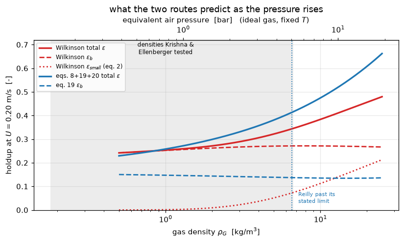
rho_G   1.3 kg/m3 (~ 1.0 bar air): Wilkinson eps 0.259 (eps_b 0.256), eqs. 8+19+20 eps 0.272 (eps_b 0.146)
rho_G   6.7 kg/m3 (~ 5.2 bar air): Wilkinson eps 0.346 (eps_b 0.271), eqs. 8+19+20 eps 0.416 (eps_b 0.137)
rho_G  13.0 kg/m3 (~10.0 bar air): Wilkinson eps 0.410 (eps_b 0.270), eqs. 8+19+20 eps 0.520 (eps_b 0.135)
rho_G  20.0 kg/m3 (~15.4 bar air): Wilkinson eps 0.456 (eps_b 0.268), eqs. 8+19+20 eps 0.608 (eps_b 0.135)

The two totals cross at rho_G = 0.85 kg/m3 (~0.7 bar of air), found on 0.1 to 70 kg/m3, the range where eq. 8 is physical.
Below it Wilkinson predicts MORE total holdup, because its overpredicted
large-bubble population outweighs its missing small one; above it, LESS,
because Reilly's eps_trans climbs steeply while Wilkinson's eps_b flattens.
Over the plotted range Wilkinson's eps_b is 1.61 to 2.01 times eq. 19's, the largest at rho_G = 12.4 kg/m3 (root of the analytic derivative),
never below it, so the two eps_b curves do not cross and the disagreement about
the TOTAL is dominated by the transition closure.
Note also that beyond rho_G = 6.5 kg/m3 the blue curves use Reilly
outside the eps_trans <= 0.32 range its authors state it was developed on.
NEITHER branch is tested by anything on this page. Krishna and Ellenberger
state the limit explicitly: their gas-density conclusion covers densities
to 6.7 kg/m3 and 'the validity of this conclusion needs to be tested for
higher gas densities'. Beyond the shaded band this figure is two
extrapolations, drawn to show where they disagree, not to settle it.
The honest limits of this page.
- The primary source was not read. Everything rests on Krishna and Ellenberger’s reprint of Eqs. 1–4, verified on 600 dpi renders but not against Wilkinson’s own paper. If they mis-set an exponent, this page inherits it. What defends against that is the dimensional identity and the figure reproductions, and nothing else. The rise-velocity groups come out exactly dimensionless, which constrains Eqs. 3 and 4; the source’s own Notation list fixes the units; and this page’s Eq. 2 reproduces the authors’ plotted evaluation of it on two different figures. The \(C^1\) continuity check does not contribute here: it reads back an exponent typed into the function being evaluated. Note too what the dimensional identity does not reach: an exponent applied to an already dimensionless group (0.757, −0.273, −0.077, 0.03, 0.077) stays dimensionless whatever its value, so those five numbers rest on the 600 dpi render alone and on nothing computed here.
- Wilkinson’s stated range of validity is unknown here. The original paper surely states one; this page can only observe where the equations behave and where they do not. Everything said about where Eq. 2 does or does not work is a statement about the formula, not a quotation of its authors, and the density at which Eq. 2 crosses a fixed level is a lower bound on adequacy and not a density at which the correlation becomes right.
- The only measurements used are the Figure 11 markers: one column, one liquid, four gases. The gas labels are unreliable, so all markers are evaluated at air density and the resulting bias is quoted with its four-gas span. The liquid-property and diameter behaviour is discussed and not tested; those are Figures 7 and 9 and neither is digitised. The diameter of the largest column (0.63 m) is quoted from
F1.4, not from a dataset. - The Figure 6 pairs are read by eye against printed ticks to two significant figures. They are plot markers and a scale for a trend the paper states in words; they are not a dataset, have no CSV or sidecar, and none of the transcription checks uses them. The claims resting on them are the decades below the measurement, the range of Reilly’s \(U_{\mathrm{trans}}\) against the measured \(U_{\mathrm{df}}\), the end-to-end bias with the \(U_{\mathrm{df}}\) read off Figure 6, and the extrapolated measured level where Eq. 2 crosses the fixed level, which is labelled a three-point reconstruction on the page. Drawing either panel as a flat band would assert a density-independence the paper explicitly denies.
- The end-to-end bias uses Reilly’s \(U_{\mathrm{trans}}\) (or the three Figure 6 readings) in place of the measured \(U_{\mathrm{df}}\) of each marker, which is not published point by point; the stand-in is within the spread quoted above.
- The total-holdup comparison uses a reference built from the measured \(\varepsilon_b\) plus Reilly’s \(\varepsilon_{df}\), because the total holdup for these runs is not published. It is indicative; the authors’ own Table 3 totals are the measurement-based version and are quoted as theirs.
- Nothing here reproduces Table 3, and no number on this page should be read as attempting to.
Reuse
Five standalone functions. wilkinson_transition, wilkinson_vb, wilkinson, reilly_transition and eq19 take SI arguments, and must take SI arguments, because two of them are unit-bound. wilkinson(U, rho_G, liquid) runs the whole correlation from a superficial velocity and returns every intermediate. Every constant is in the dictionary K; pass a modified copy as k= to test a different transcription.
Which transition closure to use. Krishna and Ellenberger recommend Reilly’s Eq. 8 with \(\varepsilon_{df} = \varepsilon_{\mathrm{trans}}\) and \(U_{df} = U_{\mathrm{trans}}\), and at atmospheric conditions that is clearly right. Do not read this page as saying that Wilkinson’s Eq. 2 takes over at high pressure: it does not. Eq. 8 exceeds Eq. 2 at every density, so there is no density at which the page’s own figure shows Eq. 2 overtaking it, and the measured dense-phase voidage rises with density too, which Eq. 2’s ceiling caps. For a pressurised column neither closure has support in this source: Eq. 8 was developed on data reaching the ceiling stated above, which SF₆ already exceeds, and it gives \(\varepsilon_{\mathrm{trans}} > 1\) at high enough density, so at the very least clip it. Eq. 8 remains the better-supported of the two, and above the SF₆ density the honest answer is that this source does not settle the question.
Which holdup correlation to use. For \(U > 0.1\) m/s and dispersion heights above 1 m, Eq. 19; see F1.4, which tests it against these same markers. Wilkinson’s value is as a structure: it is the correlation that says the split follows from a regime transition, and if you need the transition itself, it is Eq. 2 or Reilly’s Eq. 8 and nothing else in either paper. Do not evaluate Wilkinson at the plotted abscissa and read the result as an end-to-end prediction: at small excess velocity the two differ by a large factor, as the abscissa study shows.
Where the closure is consumed. F2.3 builds the S7 two-phase bubble-column reactor that needs \(\varepsilon_b\); F1.9 is the regime-transition page proper.
Related pages. F1.4 (the replacement correlation and the data), F2.3 (the reactor model), F1.9 (regime transition), F3.1 (gas–liquid reaction regimes).
Cite the origin, and the text it was read from. The correlation is Wilkinson, P. M., Spek, A. P. and van Dierendonck, L. L., Design parameters estimation for scale-up of high-pressure bubble columns, AIChE Journal 38(4) 544–554 (1992), doi:10.1002/aic.690380408. The equations used here were read from its reprint as Eqs. 1–4 of Krishna, R. and Ellenberger, J., Gas holdup in bubble column reactors operating in the churn-turbulent flow regime, AIChE Journal 42(9) 2627–2634 (1996), doi:10.1002/aic.690420923, which is also the source of the Reilly Eq. 8 closure, the Table 2 properties and the Table 3 statistics.
# Claims: prints every registered number, writes agreement.json for CI, and
# raises when a claim fails its own check or has no break row.
claims.report();   # the semicolon keeps the notebook from echoing the payload
Claims for F1.3:
eps_trans_wilkinson_air_tetradecane = 0.0028012 value rtol 1e-06
eps_trans_reilly_air_tetradecane = 0.14735 value rtol 1e-06
transition_ratio_reilly_over_wilkinson = 52.604 value rtol 1e-06
eps_trans_wilkinson_helium = 1.5058e-08 value rtol 1e-06
U_trans_wilkinson_helium_nm_s = 3.9278 value rtol 1e-06
transition_ratio_helium = 3.7881e+06 value rtol 1e-06
transition_ratio_SF6 = 4.3585 value rtol 1e-06
eps_trans_reilly_SF6 = 0.32373 value rtol 1e-06
eps_trans_wilkinson_air_water = 0.010185 value rtol 1e-06
eps_trans_reilly_air_water = 0.13665 value rtol 1e-06
water_over_tetradecane_wilkinson = 3.6361 value rtol 1e-06
tetradecane_over_water_reilly = 1.0783 value rtol 1e-06
decades_low_helium = 6.7716 value rtol 1e-06
decades_low_air = 1.6957 value rtol 1e-06
decades_low_argon = 1.412 value rtol 1e-06
reilly_eps_trans_helium_density = 0.057042 value rtol 1e-06
reilly_eps_trans_argon_density = 0.17364 value rtol 1e-06
reilly_U_trans_vs_curve_helium_density = -0.17814 value rtol 1e-06
reilly_U_trans_vs_curve_argon_density = -0.22022 value rtol 1e-06
reilly_U_trans_vs_measured_min = -0.18324 value rtol 1e-06
reilly_U_trans_vs_measured_max = 0.23391 value rtol 1e-06
rho_G_where_eq2_reaches_0p15 = 14.238 value rtol 1e-06
rho_G_where_reilly_reaches_0p32 = 6.5403 value rtol 1e-06
rho_G_where_reilly_reaches_1 = 70.232 value rtol 1e-06
rho_G_at_reilly_U_trans_peak = 15.107 value rtol 1e-06
reilly_U_trans_peak = 0.051097 value rtol 1e-06
rho_G_at_eq8_over_eq2_min = 28.592 value rtol 1e-06
eq8_over_eq2_min_ratio = 2.8538 value rtol 1e-06
eq8_exceeds_eq2_everywhere = True exact exact, margin 1.85
fig6_eps_df_exponent = 0.29508 value rtol 1e-06
measured_level_at_rho_0p15 = 0.31756 value rtol 1e-06
factor_low_at_rho_0p15 = 2.117 value rtol 1e-06
rho_G_where_totals_cross = 0.85367 value rtol 1e-06
rho_G_at_eps_b_over_eq19_max = 12.405 value rtol 1e-06
eps_b_wilkinson_over_eq19_max = 2.0106 value rtol 1e-06
eps_b_wilkinson_over_eq19_min = 1.6106 value rtol 1e-06
dimensionless_groups = 4 exact exact
dimensional_transition_groups = 3 exact exact
eq2_value_with_mPa_s_inputs = 2.9507e-153 value rtol 1e-06
continuity_limit_departure = (here 1.1e-06) bound bound <= 1e-05 [chosen]
eps_b_monotone = True exact exact
inverse_U_eps_b_0p05 = 0.016975 value rtol 1e-06
inverse_U_eps_b_0p15 = 0.075619 value rtol 1e-06
inverse_U_eps_b_0p30 = 0.28117 value rtol 1e-06
inverse_roundtrip_error = (here 1.1e-15) bound bound <= 1e-09 [tolerance]
U_where_eps_reaches_1 = 12.184 value rtol 1e-06
eps_at_U_0p5 = 0.38333 value rtol 1e-06
n_points = 63 exact exact
n_gases = 4 exact exact
wilkinson_eps_b_mean_abs_dev = 0.63942 value rtol 1e-06
wilkinson_eps_b_bias = 0.63942 value rtol 1e-06
wilkinson_eps_b_worst_dev = 1.3345 value rtol 1e-06
wilkinson_eps_b_min_dev = 0.098671 value rtol 1e-06
wilkinson_dev_gap_to_F1_4 = (here 0.0e+00) bound bound <= 1e-09 [chosen]
eq19_mean_abs_dev = 0.13831 value rtol 1e-06
eq19_bias = 0.028361 value rtol 1e-06
eq19_dev_gap_to_F1_4 = (here 0.0e+00) bound bound <= 1e-09 [chosen]
wilkinson_eps_b_bias_all_helium = 0.46814 value rtol 1e-06
V_b_shortfall_all_helium = 0.31886 value rtol 1e-06
V_b_shortfall_marker_mean_all_helium = 0.30037 value rtol 1e-06
wilkinson_eps_b_bias_all_air = 0.63942 value rtol 1e-06
V_b_shortfall_all_air = 0.39003 value rtol 1e-06
V_b_shortfall_marker_mean_all_air = 0.37382 value rtol 1e-06
wilkinson_eps_b_bias_all_argon = 0.6707 value rtol 1e-06
V_b_shortfall_all_argon = 0.40145 value rtol 1e-06
V_b_shortfall_marker_mean_all_argon = 0.38558 value rtol 1e-06
wilkinson_eps_b_bias_all_SF6 = 0.79407 value rtol 1e-06
V_b_shortfall_all_SF6 = 0.44261 value rtol 1e-06
V_b_shortfall_marker_mean_all_SF6 = 0.42791 value rtol 1e-06
wilkinson_secant_slope = 0.62062 value rtol 1e-06
measured_free_slope = 0.63611 value rtol 1e-06
deviation_corr_with_log_excess = -0.1087 value rtol 1e-06
V_small_fraction_of_V_b_mean = 0.45794 value rtol 1e-06
V_small_fraction_of_V_b_min = 0.22571 value rtol 1e-06
V_small_fraction_of_V_b_max = 0.77245 value rtol 1e-06
V_small_fraction_at_lowest_excess = 0.77245 value rtol 1e-06
eq4_second_term_larger_points = 42 exact exact, margin 0.0109
eq4_terms_equal_excess = 0.071866 value rtol 1e-06
abscissa_convention_max_effect = 0.14956 value rtol 1e-06
end_to_end_bias_helium = 0.65937 value rtol 1e-06
abscissa_effect_max_air_markers = 1.2821 value rtol 1e-06
end_to_end_bias_air = 1.0634 value rtol 1e-06
end_to_end_bias_argon = 1.1374 value rtol 1e-06
end_to_end_bias_SF6 = 1.283 value rtol 1e-06
abscissa_effect_max_all_markers = 1.3813 value rtol 1e-06
end_to_end_bias_air_fig6_U_df = 0.98988 value rtol 1e-06
small_bubble_error_mean = -0.12787 value rtol 1e-06
large_bubble_error_mean = 0.066183 value rtol 1e-06
total_holdup_error_cancellation = 0.68211 value rtol 1e-06
churn_points = 42 exact exact, margin 0.0128
churn_eps_b_dev = 0.61717 value rtol 1e-06
churn_eps_dev = 0.17106 value rtol 1e-06
table3_eps_b_wilkinson_over_replacement = 7.8125 value rtol 1e-06
table3_eps_b_over_eps_wilkinson = 5.2083 value rtol 1e-06
implied_bias_at_0p63m = 1.2833 value rtol 1e-06