# Bootstrap: the pymrm this page was checked with, and the gallery files it was
# published with. Works in a checkout, in CI and on a fresh Colab VM.
GALLERY_REF = "gallery-2026.11.10.3"  # replaced by the release tag at publication
PYMRM = ">=3.3.0,<4"  # equals meta.yaml pymrm_min_version, up to the next major
PAGE = "C2.1-xu-froment-smr"  # equals the page directory

import os, sys, urllib.request
from pathlib import Path
_shared = next((p / "shared" for p in (Path.cwd(), *Path.cwd().parents)
                if (p / "shared" / "gallery_bootstrap.py").is_file()), None)
if _shared is None:
    _shared = (Path(os.environ.get("XDG_CACHE_HOME") or Path.home() / ".cache")
               / "pymrm-gallery" / GALLERY_REF)
    _shared.mkdir(parents=True, exist_ok=True)
    urllib.request.urlretrieve(
        "https://raw.githubusercontent.com/computational-chemical-engineering/"
        f"pymrm-gallery/{GALLERY_REF}/shared/gallery_bootstrap.py",
        _shared / "gallery_bootstrap.py")
sys.path.insert(0, str(_shared))
sys.modules.pop("gallery_bootstrap", None)
from gallery_bootstrap import setup
setup(PAGE, PYMRM, GALLERY_REF); # the semicolon stops the cell echoing the pathSteam methane reforming: the Xu-Froment intrinsic kinetics
sec:C
struct:S1
struct:S2
tier:T1
data:tier2
data:tier4
phase:gas
phase:gas-solid
The most-used rate equations in reformer modelling, rebuilt from the 1989 tables and put back against the runs plotted in the paper’s own Figures 2 and 3.
Steam methane reforming: the Xu-Froment intrinsic kinetics
Catalog ID: C2.1 · Structures: S1 (0D/1D reaction network), S2 (plug flow with reaction) · Tier: T1
Almost every steam-reformer simulation published since 1989 uses the same three rate equations. They come from one paper, and getting them wrong is easy: the scan mangles the exponents, the reference temperature is not the same for all seven parameters, and two different activity factors float around the text. This page rebuilds them from the tables and puts them back against the measurements they were fitted to.
# Imports. The page's model.py is put on sys.path by setup().
import re
from dataclasses import replace

import numpy as np
import matplotlib.pyplot as plt
from IPython.display import Markdown, display
from scipy.optimize import brentq
from pymrm.checks import observed_orders
from gallery_utils import Claims, cite_data, load_data, load_meta
from model import (ATOMS, R_KJ, SPECIES, STOICH, SteamReformer, XuFroment, half_ulp,
                   partial_pressures, reference_profile, reference_solution, round_trip)

plt.rcParams.update({"figure.dpi": 110, "axes.grid": True, "grid.alpha": 0.3})
claims = Claims(PAGE.split("-")[0])
EPS = np.finfo(float).eps
BREAK = []   # (injected defect, claim, clean value, broken value, caught)


def brk(row, metric, broken):
    """One injected defect: ``broken`` is what claim ``metric`` becomes with it."""
    caught = claims.breaks(row, metric, broken)
    BREAK.append((row, metric, claims[metric], broken, caught))
Background
Steam reforming is how most of the world’s hydrogen is made. Methane and steam go into rows of tubes packed with a nickel catalyst, sitting in a fired furnace at 675-1000 K and 30 bar, and come out as synthesis gas. The tubes are the most expensive part of the plant and they fail by creep, so how fast the reaction actually runs, and therefore how much heat has to cross the tube wall and where, is a materials question as much as a chemical one.
Before 1989 most published kinetics were effective rate equations: fitted on industrial-size pellets, with the (severe) internal diffusion limitation absorbed into the constants. Those cannot be transferred to a different pellet, and they cannot be combined with a diffusion model without double-counting.
Xu and Froment set out to measure the intrinsic kinetics instead, on catalyst crushed to 0.18-0.25 mm, where they show diffusion no longer limits, and to do it mechanistically rather than by curve-fitting a power law. They enumerated 11 candidate reactions, cut them down thermodynamically, built two surface mechanisms, generated 21 candidate sets of three rate equations from them, and discriminated between the sets on 220 steam-reforming runs plus 60 runs on the reverse water-gas shift and methanation.
What survived is the triangular scheme
\[ \mathrm{I}\;\;\mathrm{CH_4 + H_2O \rightleftharpoons CO + 3H_2}, \qquad \mathrm{II}\;\;\mathrm{CO + H_2O \rightleftharpoons CO_2 + H_2}, \qquad \mathrm{III}\;\;\mathrm{CH_4 + 2H_2O \rightleftharpoons CO_2 + 4H_2}, \]
with reaction III a parallel route to CO₂ rather than CO₂ being formed only through CO. That was the paper’s substantive claim, and it came from the data: the ratio \(V(\mathrm{II})\) does not extrapolate to the origin as space time goes to zero, so some CO₂ must be produced directly from methane.
The published model
Rate equations (the paper’s Eqs. 3). All three share one denominator, because all three are assumed to occur on the same active sites:
\[ r_1 = \frac{k_1}{p_{\mathrm{H_2}}^{2.5}} \left( p_{\mathrm{CH_4}} p_{\mathrm{H_2O}} - \frac{p_{\mathrm{H_2}}^{3} p_{\mathrm{CO}}}{K_1} \right) \Big/ \mathrm{DEN}^2 \]
\[ r_2 = \frac{k_2}{p_{\mathrm{H_2}}} \left( p_{\mathrm{CO}} p_{\mathrm{H_2O}} - \frac{p_{\mathrm{H_2}} p_{\mathrm{CO_2}}}{K_2} \right) \Big/ \mathrm{DEN}^2 \]
\[ r_3 = \frac{k_3}{p_{\mathrm{H_2}}^{3.5}} \left( p_{\mathrm{CH_4}} p_{\mathrm{H_2O}}^{2} - \frac{p_{\mathrm{H_2}}^{4} p_{\mathrm{CO_2}}}{K_3} \right) \Big/ \mathrm{DEN}^2 \]
\[ \mathrm{DEN} = 1 + K_{\mathrm{CO}} p_{\mathrm{CO}} + K_{\mathrm{H_2}} p_{\mathrm{H_2}} + K_{\mathrm{CH_4}} p_{\mathrm{CH_4}} + K_{\mathrm{H_2O}} \frac{p_{\mathrm{H_2O}}}{p_{\mathrm{H_2}}} \]
There is no \(K_{\mathrm{CO_2}}\) term. It was never statistically significant, from either data set, and the paper says so explicitly. Adding one is a common way to silently change the model.
Species rates (Eq. 4), for steam reforming:
\[ r_{\mathrm{CO}} = r_1 - r_2, \qquad r_{\mathrm{CO_2}} = r_2 + r_3, \qquad r_{\mathrm{CH_4}} = r_1 + r_3 \]
Reactor (Eq. 1). The kinetic runs were done in an integral fixed bed, isothermal and isobaric, integrated in the space time \(W/F^{0}_{\mathrm{CH_4}}\):
\[ \frac{\mathrm{d}x_{\mathrm{CH_4}}}{\mathrm{d}(W/F^{0}_{\mathrm{CH_4}})} = r_{\mathrm{CH_4}}, \qquad \frac{\mathrm{d}x_{\mathrm{CO_2}}}{\mathrm{d}(W/F^{0}_{\mathrm{CH_4}})} = r_{\mathrm{CO_2}}, \qquad x = 0 \;\text{at}\; W/F^{0}_{\mathrm{CH_4}} = 0 . \]
Two of the three species rates are independent, so two conversions describe the whole composition: \(x_{\mathrm{CH_4}}\), the total methane converted, and \(x_{\mathrm{CO_2}}\), the part of it that ended up as CO₂. Per mol of methane fed, CH₄ is \(1-x_{\mathrm{CH_4}}\), H₂O is \(s - x_{\mathrm{CH_4}} - x_{\mathrm{CO_2}}\), H₂ is \(h + 3x_{\mathrm{CH_4}} + x_{\mathrm{CO_2}}\), CO is \(x_{\mathrm{CH_4}} - x_{\mathrm{CO_2}}\) and CO₂ is \(x_{\mathrm{CO_2}}\), with \(s\) and \(h\) the feed ratios H₂O/CH₄ and H₂/CH₄.
| symbol | name in the code |
|---|---|
| \(x_{\mathrm{CH_4}}, x_{\mathrm{CO_2}}\) | u[:, 0], u[:, 1] of SteamReformer |
| \(W/F^{0}_{\mathrm{CH_4}}\) | tau |
| \(k_i, K_j\) | XuFroment.constants(T) |
| \(K_1, K_2, K_3\) | XuFroment.equilibrium(T) |
| \(r_1, r_2, r_3\) | XuFroment.rates(...) |
| \(s, h, p_t\) | sr, hr, p_t |
Parameters and assumptions
Assumptions: isothermal and isobaric plug flow; intrinsic kinetics (the paper demonstrates no internal limitation at 0.18-0.25 mm and calculates external transport to be negligible); ideal gas; no carbon deposition, which the thermodynamic analysis rules out at these conditions; and the catalyst held at a fixed activity level, which is how the authors corrected their space times.
Three traps in this paper. Each one silently changes the answer:
- The reference temperature is not the same for all parameters. \(T_r = 648\) K for \(k_1, k_2, k_3, K_{\mathrm{CO}}\) and \(K_{\mathrm{H_2}}\), but \(T_r = 823\) K for \(K_{\mathrm{CH_4}}\) and \(K_{\mathrm{H_2O}}\). Using one reference for all seven biases the temperature dependence (Validation, check 1, prints by how much).
- Three activity levels. Table 6 is footnoted reference activity, the partially deactivated catalyst. Multiply the rate coefficients by 1.225 for the reverse water-gas shift and methanation reference level (the curves in the paper’s Figures 4 and 5 were drawn that way), and by 2.246 for fresh catalyst. The steam-reforming data used here need neither.
- The exponents do not survive OCR. In the PDF text layer \(8.664 \times 10^{-7}\) comes out as
8.664 lo-'. Every parameter below was read from a 600 dpi render of the printed page instead, and none was repaired by inference: a misread exponent is a wrong rate constant with no outward sign. The Table 5 to Table 6 round trip in the validation section is the check on that reading.
What the paper does not give: the equilibrium constants. \(K_1\), \(K_2\) and \(K_3\) appear in the rate equations but are tabulated nowhere in it, so they must come from elsewhere. This page uses the correlations usually quoted with these kinetics (Twigg, Catalyst Handbook, 2nd ed., 1989), \(K_1 = \exp(-26830/T + 30.114)\) bar², \(K_2 = \exp(4400/T - 4.036)\) and \(K_3 = K_1 K_2\), and then tests them against the paper’s own Table 7 reaction enthalpies, which is the strongest consistency check available without importing a thermodynamic database.
par = load_data("xu-froment-1989-parameters.csv", page=PAGE)
par_txt = load_data("xu-froment-1989-parameters.csv", page=PAGE, dtype=str)  # as printed
obs = load_data("xu-froment-1989-conversion.csv", page=PAGE)
obs_meta = load_meta("xu-froment-1989-conversion.csv", page=PAGE)
cond = obs_meta["conditions"]

P_T = float(cond["pressure_bar"])     # total pressure, bar (figure captions)
SR = float(cond["h2o_ch4_molar"])     # H2O/CH4 in the feed (figure captions)
HR = float(cond["h2_ch4_molar"])      # H2/CH4 in the feed (Table 1)
TEMPS = [float(T) for T in cond["temperatures_K"]]   # K, the four curves
TAU_MAX = 0.45                        # g_cat h / mol_CH4, beyond the last run
N_TAU = 1000                          # cells in tau (Validation, check 4)
kin = XuFroment.from_table(par)       # Table 6 A, Table 5 E, the correlation above
print(f"p_t = {P_T} bar, H2O/CH4 = {SR}, H2/CH4 = {HR}, T = {TEMPS} K")
p_t = 10.0 bar, H2O/CH4 = 3.0, H2/CH4 = 1.25, T = [773.0, 798.0, 823.0, 848.0] KThe data
Two datasets, both extracted from the paper and both carrying a provenance sidecar.
The parameters are Tables 5 and 6 read off a 600 dpi page render. The measurements are the experimental markers of Figures 2 and 3: total methane conversion and conversion into CO₂ against space time, at the conditions printed above, at four temperatures. The smooth curves on those figures are the authors’ own model and were deliberately not extracted, so what follows compares this implementation against measurements rather than against someone else’s fit. The sidecar records the cross-figure pairing of the two digitisations, the carbon closure \(x_{\mathrm{CO_2}} \le x_{\mathrm{CH_4}}\) and one merged glyph in Figure 2 that was recorded once rather than guessed.
print(par[["symbol", "A", "E_or_dH_kJ_per_mol", "value_at_Tref", "T_ref_K"]]
      .to_string(index=False))
print()
print(obs.groupby(["quantity", "temperature_K"]).size().unstack().to_string())
N_OBS = len(obs)
print(f"\n{N_OBS} measurements ({(obs.quantity == 'x_CH4').sum()} x_CH4, "
      f"{(obs.quantity == 'x_CO2').sum()} x_CO2), W/F from {obs.W_F.min():.3f} to "
      f"{obs.W_F.max():.3f} g_cat h/mol_CH4")
claims.value("W_F_measured_max", obs.W_F.max(), unit="g_cat h/mol_CH4",
             note="the last measured space time; the computed bed ends at TAU_MAX")
_err = " ".join(obs_meta["acquisition"]["estimated_error"].split())
brk("the bed outlet TAU_MAX read as the last measurement", "W_F_measured_max", TAU_MAX)
print("digitisation error (sidecar): " + _err)
claims.value("digitisation_error_conversion",
             float(re.search(r"\+/-\s*([0-9.]+) in conversion", _err).group(1)),
             note="read from the data sidecar's estimated_error")
brk("regular expression matching the W/F error instead of the conversion error",
    "digitisation_error_conversion",
    float(re.search(r"\+/-\s*[0-9.]+ in conversion and \+/-\s*([0-9.]+) in W/F", _err).group(1)))
print(cite_data(obs_meta))
symbol A E_or_dH_kJ_per_mol value_at_Tref T_ref_K
k1 4.225000e+15 240.10 0.000184 648
k2 1.955000e+06 67.13 7.558000 648
k3 1.020000e+15 243.90 0.000022 648
K_CO 8.230000e-05 -70.65 40.910000 648
K_H2 6.120000e-09 -82.90 0.029600 648
K_CH4 6.650000e-04 -38.28 0.179100 823
K_H2O 1.770000e+05 88.68 0.415200 823
temperature_K 773 798 823 848
quantity
x_CH4 6 5 13 6
x_CO2 6 5 14 6
61 measurements (30 x_CH4, 31 x_CO2), W/F from 0.128 to 0.405 g_cat h/mol_CH4
digitisation error (sidecar): +/- 0.0006 in conversion and +/- 0.0007 in W/F, dominated by placing the centre of a ~20 px glyph that overlaps a ~10 px curve, plus the tick residuals quoted above.
Xu, J.; Froment, G. F. (1989) — AIChE Journal 35(1) 88-96 — doi:10.1002/aic.690350109 — digitised from Figure 2 (total methane conversion) and Figure 3 (methane converted to CO2), journal page 89PyMRM implementation
The reactor is pure convection with a source: \(\mathrm{d}(v\,x)/\mathrm{d}\tau
= r\) with \(v = 1\) and \(\tau = W/F^{0}_{\mathrm{CH_4}}\). That is construct_convflux_upwind followed by construct_div (nu=0), exactly as for a plug flow in space: the coordinate being a space time rather than a length changes nothing about the operators. Both are assembled once in SteamReformer._build_operators.
Boundary conditions, on the outward normal. At the inlet (\(-\tau\)) the conversions are zero, \(x = 0\): {"a": 0, "b": 1, "d": 0}. The outlet is a pure convective outflow, {"outflow": True}: what leaves is what the last cell holds, and no condition is imposed on the profile. The outlet value is read on the outlet face with compute_boundary_values (SteamReformer.outlet).
State and Jacobian. The state is (n_tau, 2), space time first and the two conversions last. The source at a cell depends only on that cell’s two conversions, so the default NumJac(shape) stencil, which couples the last axis in full, has exactly the structure of the true Jacobian: one \(2\times2\) block per cell. Nothing here needs axes_diagonals; the coupling between cells comes in analytically through the convection operator. newton starts from \(x = 0\) and solve raises unless it converges.
What first-order upwind means here. With \(v = 1\) the upwind balance of cell \(i\) is \((u_i - u_{i-1})/\Delta\tau = r(u_i)\): backward Euler in \(\tau\). Reading a measurement at an arbitrary \(\tau\) needs an interpolation, and two readings are natural: between cell centres, or between the upwind face values (each cell value placed at its downstream face). Both are first order; check 4 measures which one is closer to the exact profile.
def solve_all(k, n_tau=N_TAU, **kw):
    """The four isothermal reactors of Figures 2 and 3 for kinetics ``k``."""
    return {T: SteamReformer(k, T, P_T, SR, HR, tau_max=TAU_MAX, n_tau=n_tau, **kw).solve()
            for T in TEMPS}


models = solve_all(kin)
for T, m in models.items():
    print(f"T = {T:.0f} K   Newton iterations: {m.result.nit}   "
          f"backward error (here {m.backward_error():.1e})")
T = 773 K Newton iterations: 4 backward error (here 1.9e-16)
T = 798 K Newton iterations: 4 backward error (here 3.1e-16)
T = 823 K Newton iterations: 4 backward error (here 1.3e-15)
T = 848 K Newton iterations: 5 backward error (here 2.2e-16)Results
The two panels are the paper’s Figures 2 and 3 rebuilt: markers are the digitised measurements, lines are this implementation. Nothing was fitted: every parameter is Table 6 as printed.
COL = {773.0: "tab:blue", 798.0: "tab:green", 823.0: "tab:orange", 848.0: "tab:red"}
MRK = {773.0: "o", 798.0: "^", 823.0: "s", 848.0: "D"}
FIELD = {"x_CH4": 0, "x_CO2": 1}

fig, axes = plt.subplots(1, 2, figsize=(11.5, 4.4), sharex=True)
for ax, (q, lab) in zip(axes, [("x_CH4", r"$x_{\mathrm{CH_4}}$, total methane converted"),
                               ("x_CO2", r"$x_{\mathrm{CO_2}}$, methane converted into CO$_2$")]):
    for T in TEMPS:
        m = models[T]
        ax.plot(m.tau_c, m.u[:, FIELD[q]], color=COL[T], lw=1.6)
        s = obs[(obs.quantity == q) & (obs.temperature_K == T)]
        ax.plot(s.W_F, s.value, MRK[T], color=COL[T], ms=5, mfc="none", mew=1.3,
                label=f"{T:.0f} K")
    ax.set_xlabel(r"$W/F^{0}_{\mathrm{CH_4}}$  (g$_\mathrm{cat}$ h / mol$_{\mathrm{CH_4}}$)")
    ax.set_ylabel(lab + "  (-)")
    ax.set_xlim(0, TAU_MAX)
    ax.set_ylim(0, None)
handles, labels = axes[0].get_legend_handles_labels()
fig.legend(handles, labels, loc="lower center", ncol=4, fontsize=9, frameon=False,
           title="markers: measured   ·   lines: pymrm")
fig.suptitle("Xu & Froment (1989) Figures 2 and 3, reproduced from Table 6", fontsize=11)
fig.tight_layout(rect=(0, 0.13, 1, 1))
plt.show()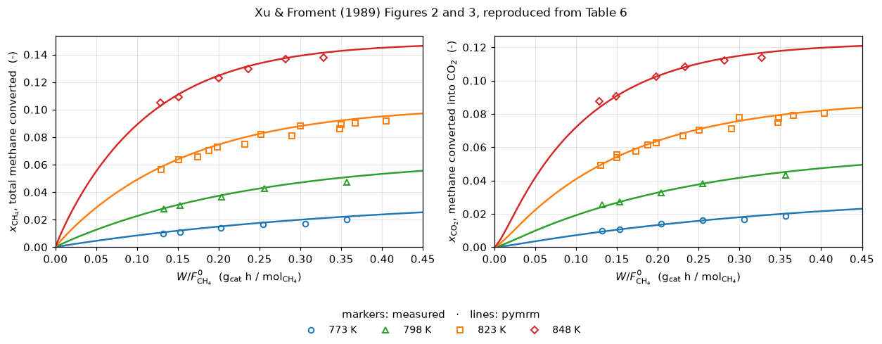
def deviations(ms, read="centre"):
    """Model minus measurement at every digitised point, in the order of ``obs``."""
    return np.array([ms[r.temperature_K].at(r.W_F, FIELD[r.quantity], read=read) - r.value
                     for r in obs.itertuples()])


res = obs.copy()
res["dev"] = deviations(models)
res["model"] = res.value + res.dev
summary = (res.groupby(["quantity", "temperature_K"])["dev"]
             .agg(n="size", MAD=lambda s: s.abs().mean(),
                  worst=lambda s: s.abs().max(), bias="mean").round(5))
print(summary.to_string())
print(f"\noverall: n = {len(res)}   MAD = {res.dev.abs().mean():.5f}   "
      f"worst = {res.dev.abs().max():.5f}   bias = {res.dev.mean():+.5f}")
n MAD worst bias
quantity temperature_K
x_CH4 773 6 0.00170 0.00322 0.00170
798 5 0.00146 0.00387 0.00146
823 13 0.00282 0.00582 0.00279
848 6 0.00208 0.00368 0.00137
x_CO2 773 6 0.00073 0.00174 0.00030
798 5 0.00081 0.00206 0.00019
823 14 0.00153 0.00435 0.00104
848 6 0.00137 0.00390 -0.00003
overall: n = 61 MAD = 0.00172 worst = 0.00582 bias = +0.00130Validation
Five checks. The first two test the parameters, the part of this page that a bad page render would silently corrupt; the third tests the mole bookkeeping; the fourth the discretisation and the solver against an independent integration; the fifth the model against the measurements. Every number is registered as a claim, and each check injects the defects it is meant to catch, through an argument or a parameter, and prints whether the claim’s own check fails. The break table at the end of “What pymrm adds” collects every row.
A blind spot in the obvious summary of check 1. The worst per-row round-trip deviation is a max() over seven rows, and its baseline scatter is set by the printed precision of the activation energies: E is given to 0.1 kJ/mol, and at \(T_r = 648\) K that alone is worth 0.93 % on A. So k1 and k3 carry the largest deviations in the table with nothing wrong at all, and a single-digit slip that lands below that ceiling leaves the worst deviation unchanged. A max() is only as sharp as its own baseline scatter. The page therefore also normalises each row by its own printed precision and sums the seven ratios, a statistic that every row reaches.
# 1. Table 5 -> Table 6 round trip. A = value(T_ref) exp(E / (R T_ref)) for the rate
#    coefficients, and the same with dH for the adsorption constants. It tests both
#    readings at once, and the split reference temperature, which is in the formula.
#    The printed digits come from the CSV read as text, so the precision of every
#    entry is the precision it was printed with.
ROWS = [dict(symbol=r.symbol, A=r.A, E=r.E_or_dH_kJ_per_mol, val=r.value_at_Tref,
             T_ref=float(r.T_ref_K)) for r in par_txt.itertuples()]


def rt_metrics(rows, T_ref=None):
    rt = round_trip(rows, T_ref=T_ref)
    return (max(r["rel_pct"] for r in rt), max(r["ratio"] for r in rt),
            sum(r["ratio"] for r in rt), rt)


def rows_with(symbol, key, new):
    """The printed rows with one entry of ``symbol`` replaced by the string ``new``."""
    out = [dict(r) for r in ROWS]
    for r in out:
        if r["symbol"] == symbol:
            r[key] = new
    return out


RT_WORST_PCT, RT_WORST_RATIO, RT_RATIO_SUM, RT = rt_metrics(ROWS)
print("1. Table 5 -> Table 6 round trip, each row against its own printed precision")
print(f"   {'symbol':6s} {'T_ref':>6s} {'A':>10s} {'A computed':>11s} {'rel %':>8s} "
      f"{'bound %':>8s} {'ratio':>7s}")
for r in RT:
    print(f"   {r['symbol']:6s} {r['T_ref']:6.0f} {r['A']:10.4g} {r['A_computed']:11.4g} "
          f"{r['rel_pct']:8.4f} {r['bound_pct']:8.4f} {r['ratio']:7.3f}")
E_SHARE = half_ulp(ROWS[0]["E"]) / (R_KJ * ROWS[0]["T_ref"]) * 100
print(f"   worst deviation {RT_WORST_PCT:.4f} %; half a unit of E = {ROWS[0]['E']} kJ/mol "
      f"at {ROWS[0]['T_ref']:.0f} K is {E_SHARE:.2f} % on A by itself")
print(f"   worst ratio to printed precision {RT_WORST_RATIO:.2f}, sum over the seven rows "
      f"{RT_RATIO_SUM:.3f}")

# The same round trip with 648 K forced on every parameter: the split reference
# temperature is not a detail one can round off.
TREF = {r["symbol"]: r["A_computed"] / r["A"] for r in round_trip(ROWS, T_ref=648.0)}
print("   with 648 K for every parameter:   "
      + "   ".join(f"{s} off by a factor of {TREF[s]:.3g}" for s in ("K_CH4", "K_H2O")))

claims.value("param_round_trip_worst_pct", RT_WORST_PCT, unit="%")
claims.value("param_round_trip_worst_ratio_to_precision", RT_WORST_RATIO)
claims.value("param_round_trip_ratio_sum", RT_RATIO_SUM)
claims.value("e_precision_share_pct", E_SHARE, unit="%",
             note="half a unit of k1's printed E at 648 K, as a share of A")
claims.value("tref_slip_factor_K_CH4", TREF["K_CH4"])
claims.value("tref_slip_factor_K_H2O", TREF["K_H2O"])

print("\n   injected transcription defects (each re-runs the round trip):")
print(f"   {'injected defect':46s}{'worst %':>10}{'worst ratio':>13}{'sum ratios':>12}")
print(f"   {'as printed':46s}{RT_WORST_PCT:10.4f}{RT_WORST_RATIO:13.2f}{RT_RATIO_SUM:12.3f}")
RT_DEFECTS = [("K_CO", "A", "8.32e-5"), ("k3", "A", "1.002e15"), ("K_H2O", "A", "1.71e5"),
              ("k2", "A", "1.965e6"), ("k1", "A", "4.226e15"), ("k1", "E", "240.2"),
              ("K_CH4", "val", "0.1719"), ("k1", "E", "241.1"), ("k1", "A", "4.225e14"),
              ("K_CH4", "T_ref", 648.0)]
for sym, key, new in RT_DEFECTS:
    old = next(r[key] for r in ROWS if r["symbol"] == sym)
    lab = f"{sym} {key} {old} -> {new} (rows_with('{sym}', '{key}', {new!r}))"
    w, wr, sm, _ = rt_metrics(rows_with(sym, key, new))
    brk(lab, "param_round_trip_worst_pct", w)
    brk(lab, "param_round_trip_worst_ratio_to_precision", wr)
    brk(lab, "param_round_trip_ratio_sum", sm)
    print(f"   {lab[:46]:46s}{w:10.4f}{wr:13.2f}{sm:12.3f}")
_sum_rows = [c for r, mt, _, _, c in BREAK if mt == "param_round_trip_ratio_sum"]
_max_rows = [c for r, mt, _, _, c in BREAK if mt == "param_round_trip_worst_pct"]
print(f"   the sum fails its check for {sum(_sum_rows)} of {len(_sum_rows)} rows, the worst "
      f"deviation for {sum(_max_rows)} of {len(_max_rows)}")
_r = rows_with("k1", "E", "240.10")
brk("k1 E printed as 240.10 (one more digit)", "e_precision_share_pct",
    half_ulp(_r[0]["E"]) / (R_KJ * _r[0]["T_ref"]) * 100)
for sym, new in (("K_CH4", "-38.82"), ("K_H2O", "89.68")):
    old = next(r["E"] for r in ROWS if r["symbol"] == sym)
    f = {r["symbol"]: r["A_computed"] / r["A"]
         for r in round_trip(rows_with(sym, "E", new), T_ref=648.0)}
    brk(f"{sym} E {old} -> {new} (rows_with('{sym}', 'E', {new!r}))",
        f"tref_slip_factor_{sym}", f[sym])
1. Table 5 -> Table 6 round trip, each row against its own printed precision
symbol T_ref A A computed rel % bound % ratio
k1 648 4.225e+15 4.171e+15 1.2844 0.9671 1.328
k2 648 1.955e+06 1.949e+06 0.2900 0.1250 2.320
k3 648 1.02e+15 1.005e+15 1.4432 0.9999 1.443
K_CO 648 8.23e-05 8.253e-05 0.2761 0.1658 1.665
K_H2 648 6.12e-09 6.146e-09 0.4181 0.1914 2.184
K_CH4 823 0.000665 0.0006659 0.1403 0.1762 0.797
K_H2O 823 1.77e+05 1.765e+05 0.2574 0.3676 0.700
worst deviation 1.4432 %; half a unit of E = 240.1 kJ/mol at 648 K is 0.93 % on A by itself
worst ratio to printed precision 2.32, sum over the seven rows 10.438
with 648 K for every parameter: K_CH4 off by a factor of 0.221 K_H2O off by a factor of 33
injected transcription defects (each re-runs the round trip):
injected defect worst % worst ratio sum ratios
as printed 1.4432 2.32 10.438
K_CO A 8.23e-5 -> 8.32e-5 (rows_with('K_CO', ' 1.4432 4.90 13.670
k3 A 1.020e15 -> 1.002e15 (rows_with('k3', 'A' 1.2844 2.32 9.321
K_H2O A 1.77e5 -> 1.71e5 (rows_with('K_H2O', ' 3.2424 8.59 18.326
k2 A 1.955e6 -> 1.965e6 (rows_with('k2', 'A', 1.4432 6.39 14.504
k1 A 4.225e15 -> 4.226e15 (rows_with('k1', 'A' 1.4432 2.32 10.462
k1 E 240.1 -> 240.2 (rows_with('k1', 'E', '240 1.4432 2.32 9.694
K_CH4 val 0.1791 -> 0.1719 (rows_with('K_CH4', 3.8854 21.91 31.550
k1 E 240.1 -> 241.1 (rows_with('k1', 'E', '241 18.8496 19.49 28.601
k1 A 4.225e15 -> 4.225e14 (rows_with('k1', 'A' 887.1560 917.38 926.486
K_CH4 T_ref 823.0 -> 648.0 (rows_with('K_CH4', 77.8971 397.61 407.251
the sum fails its check for 9 of 10 rows, the worst deviation for 6 of 10The first column of that table is the blind spot made visible: several single-digit slips leave the worst deviation where it is, and the k3 transposition, in the row that sets the maximum, moves it down. The sum of per-row ratios moves by more than its 5 % check for every injection but one, and that one is a change of one unit in the fourth significant figure of k1’s preexponential, below the printed precision, so no round trip built from these digits can resolve it. Compare the sum, not the maximum, when re-reading these tables.
# 2. Equilibrium correlation against the paper's own thermodynamics.
#    d ln K / d(1/T) = -dH/R, so the correlation slopes ARE reaction enthalpies and
#    can be compared with Table 7 (values at 948 K).
TABLE7 = {"I": 224.0, "II": -37.3, "III": 187.5}   # kJ/mol at 948 K, the paper's Table 7


def eq_worst_pct(k):
    dh = k.vant_hoff_enthalpies()
    return max(abs(dh[r] - TABLE7[r]) / abs(TABLE7[r]) * 100 for r in TABLE7)


print("2. van 't Hoff slopes of K_i against Xu & Froment Table 7 (948 K)")
for r, v in kin.vant_hoff_enthalpies().items():
    print(f"   dH_{r:<3s} correlation {v:8.2f}   paper {TABLE7[r]:8.2f} kJ/mol   "
          f"{abs(v - TABLE7[r]) / abs(TABLE7[r]) * 100:5.2f} %")
EQ_WORST = eq_worst_pct(kin)
claims.value("equilibrium_vs_table7_worst_pct", EQ_WORST, unit="%")
print(f"   worst {EQ_WORST:.2f} %; K3 = K1 K2 closes the triangle by construction")
a1, b1, a2, b2 = kin.eq
for lab, eq in ((f"K1 slope a1 {a1:g} -> 26380 (transposition)", (26380.0, b1, a2, b2)),
                (f"K2 slope a2 {a2:g} -> 4040 (transposition)", (a1, b1, 4040.0, b2)),
                (f"K1 intercept b1 {b1:g} -> {b1 + 1:g} (K1 x e)", (a1, b1 + 1, a2, b2)),
                (f"K2 intercept b2 {b2:g} -> {b2 + 1:g} (K2 x e)", (a1, b1, a2, b2 + 1))):
    w = eq_worst_pct(replace(kin, eq=eq))
    brk(lab + " (XuFroment(eq=...))", "equilibrium_vs_table7_worst_pct", w)
    print(f"   {lab:44s} check 2 worst {w:5.2f} %")
2. van 't Hoff slopes of K_i against Xu & Froment Table 7 (948 K)
dH_I correlation 223.06 paper 224.00 kJ/mol 0.42 %
dH_II correlation -36.58 paper -37.30 kJ/mol 1.93 %
dH_III correlation 186.48 paper 187.50 kJ/mol 0.54 %
worst 1.93 %; K3 = K1 K2 closes the triangle by construction
K1 slope a1 26830 -> 26380 (transposition) check 2 worst 2.54 %
K2 slope a2 4400 -> 4040 (transposition) check 2 worst 9.95 %
K1 intercept b1 30.114 -> 31.114 (K1 x e) check 2 worst 1.93 %
K2 intercept b2 -4.036 -> -3.036 (K2 x e) check 2 worst 1.93 %What check 2 cannot see. Only the slopes are compared. The two intercepts drop out of \(\mathrm{d}\ln K/\mathrm{d}(1/T)\) entirely, so a +1 slip in either multiplies that \(K\) by \(e\) at every temperature and check 2 does not move at all: the two intercept rows above are its blind spot, shown rather than assumed. What sees them is check 5, the comparison against the measurements.
# 3. Atom balances along the reactor. The conversions are defined so that C, H and
#    O balance identically for the stoichiometry of the three reactions; this checks
#    the mole bookkeeping (model.STOICH), not the solver.
def atom_gap(ms, stoich=STOICH):
    """Largest |atoms(profile) - atoms(feed)| over every cell and reactor, mol per mol CH4 fed."""
    return max(float(np.abs(ATOMS @ (stoich @ m.u.T)).max()) for m in ms.values())


ATOM_GAP = atom_gap(models)
P_MIN = min(min(float(np.min(p)) for p in partial_pressures(m.u[:, 0], m.u[:, 1], P_T, SR, HR))
            for m in models.values()) / P_T
print(f"3. C, H and O balance along all four reactors to (here {ATOM_GAP:.1e}) mol per mol CH4 fed")
print(f"   smallest partial pressure over every cell and species: (here {P_MIN:.1e}) of p_t, positive")
claims.bound("atom_balance_worst", ATOM_GAP, max=1e-12, basis="identity",
             note="atoms of STOICH @ (x_CH4, x_CO2), every cell of the four reactors")
claims.bound("min_partial_pressure_rel", P_MIN, min=0.0, basis="theory", structural=True,
             note="every rate vanishes as one of its reactants does, so no pressure crosses "
                  "zero; the stoichiometry row below does not make one negative")
_s = STOICH.copy(); _s[2] = (3.0, 0.0)
brk("H2 formed as 3 x_CH4, no x_CO2 term (stoich row H2 = (3, 0))", "atom_balance_worst",
    atom_gap(solve_all(replace(kin, stoich=_s)), _s))
_s = STOICH.copy(); _s[3] = (1.0, -2.0)
_ms = solve_all(replace(kin, stoich=_s))
brk("CO formed as x_CH4 - 2 x_CO2 (stoich row CO = (1, -2))", "min_partial_pressure_rel",
    min(min(float(np.min(p)) for p in partial_pressures(m.u[:, 0], m.u[:, 1], P_T, SR, HR, _s))
        for m in _ms.values()) / P_T)
3. C, H and O balance along all four reactors to (here 2.2e-16) mol per mol CH4 fed
smallest partial pressure over every cell and species: (here 2.5e-06) of p_t, positiveCheck 4: the discretisation, against an independent integration. The same two ODEs are integrated by scipy.integrate.solve_ivp (Radau, implicit Runge-Kutta with its own step control, at rtol 1e-12), and both routes are read at every one of the measured space times at every temperature. The routes share the rate function and nothing else: no grid, no Jacobian, no linear solver. The finite-volume profile is then refined (500 to 4000 cells) and the observed order is taken from successive differences of all the measured-point values together, with a check that the finest difference is far above round-off.
def ref_at_obs(k=kin, rtol=1e-12):
    """The Radau route at every measured point, in the order of ``obs``."""
    out = np.empty(len(obs))
    for T in TEMPS:
        sel = (obs.temperature_K == T).to_numpy()
        prof = reference_profile(k, T, obs.W_F[sel].to_numpy(), P_T, SR, HR, rtol=rtol)
        out[sel] = prof[np.arange(sel.sum()), obs.quantity[sel].map(FIELD).to_numpy()]
    return out


REF_OBS = ref_at_obs()
REF_TOL_GAP = float(np.abs(ref_at_obs(rtol=1e-10) - REF_OBS).max())
MODEL_OBS = res.model.to_numpy()


def disc_error(ms, read="centre"):
    return float(np.abs(obs.value.to_numpy() + deviations(ms, read) - REF_OBS).max())


DISC = disc_error(models)
DISC_FACE = disc_error(models, "face")
MAD = float(res.dev.abs().mean())
print("4. finite volumes against Radau at the measured points, n_tau = "
      f"{N_TAU}: max |difference| {DISC:.2e} (centre read), {DISC_FACE:.2e} (face read)")
print(f"   = {DISC / MAD * 100:.1f} % of the mean deviation from the data; Radau rtol 1e-10 "
      f"against 1e-12 (here {REF_TOL_GAP:.0e})")
claims.value("disc_error_max_n1000", DISC,
             note="max over the measured points of |finite volumes - Radau|, centre read")
claims.value("disc_error_share_of_mad_pct", DISC / MAD * 100, unit="%")
claims.bound("radau_reference_tolerance_gap", REF_TOL_GAP, max=1e-8, basis="tolerance",
             note="Radau at rtol 1e-10 against 1e-12, at the measured points")
for lab, ms, rd in (("face read instead of centre read (at(..., read='face'))", models, "face"),
                    ("a quarter of the cells (n_tau = 250)", solve_all(kin, 250), "centre")):
    brk(lab, "disc_error_max_n1000", disc_error(ms, rd))
    brk(lab, "disc_error_share_of_mad_pct", disc_error(ms, rd) / MAD * 100)
brk("Radau reference at rtol 1e-5 (reference_profile(..., rtol=1e-5))",
    "radau_reference_tolerance_gap", float(np.abs(ref_at_obs(rtol=1e-5) - REF_OBS).max()))

NS = (500, 1000, 2000, 4000)
LADDER = {n: solve_all(kin, n) for n in (*NS, 4001)}
OO = observed_orders(lambda n: obs.value.to_numpy() + deviations(LADDER[n]), NS)
FINEST = float(np.abs(OO["values"][-1] - OO["values"][-2]).max())
print("   refinement at the measured points: max |change| "
      + ", ".join(f"{np.abs(OO['values'][i + 1] - OO['values'][i]).max():.2e}"
                  for i in range(len(NS) - 1))
      + "; observed orders " + ", ".join(f"{o:.3f}" for o in OO["orders"]))
print(f"   finest change {FINEST:.1e} = {FINEST / (NS[-1] * EPS):.1e} times n eps at {NS[-1]} cells")
claims.bound("grid_order_observed", OO["orders"][-1], min=0.95, max=1.05, basis="theory",
             note="first-order upwind, successive differences of all measured-point values, "
                  "1000 to 4000 cells")
claims.bound("grid_finest_over_roundoff", FINEST / (NS[-1] * EPS), min=1e4, basis="theory",
             note="finest ladder change over n eps (the upwind operator's condition grows as n)")
_oo = observed_orders(lambda n: obs.value.to_numpy() + deviations(LADDER[n], "nearest"), NS)
brk("nearest cell value instead of interpolation (at(..., read='nearest'))",
    "grid_order_observed", _oo["orders"][-1])
brk("ladder whose last rung is 4001 cells after 4000", "grid_finest_over_roundoff",
    float(np.abs(obs.value.to_numpy() + deviations(LADDER[4001])
                 - OO["values"][-1]).max()) / (4001 * EPS))

BE_WORST = max(m.backward_error() for m in models.values())
claims.bound("newton_backward_error_worst", BE_WORST, max=1e-8, basis="tolerance",
             note="pymrm.checks.residual_check over the four reactors; newton backward_tol 1e-8")
brk("Newton stopped after one iteration (solve(maxfev=1, strict=False))",
    "newton_backward_error_worst",
    max(SteamReformer(kin, T, P_T, SR, HR, TAU_MAX, N_TAU).solve(maxfev=1, strict=False)
        .backward_error() for T in TEMPS))
4. finite volumes against Radau at the measured points, n_tau = 1000: max |difference| 4.14e-05 (centre read), 1.12e-04 (face read)
= 2.4 % of the mean deviation from the data; Radau rtol 1e-10 against 1e-12 (here 1e-12)
refinement at the measured points: max |change| 4.13e-05, 2.07e-05, 1.04e-05; observed orders 0.999, 0.997
finest change 1.0e-05 = 1.2e+07 times n eps at 4000 cellsThe two readings of the same upwind solution differ by a factor printed above, and the centre read is the closer one, at every grid of the ladder: backward Euler places each cell value a little behind the exact profile, and reading it half a cell upstream, at the centre, cancels part of that lag. The page reads at the centres. On 1000 cells the discretisation error at the measured points is a small fraction of the deviation from the data, and below the digitisation error of the sidecar (printed under The data), so it does not decide anything that follows.
# 5. Against the measurements, and the defects only the measurements can see.
LONG = 0.28   # W/F above which the reactions approach equilibrium (bins below)
BINS = [(0.12, 0.20), (0.20, LONG), (LONG, 0.42)]


def data_metrics(dev):
    """Deviation metrics from model-minus-measurement values in the order of ``obs``."""
    d = obs.assign(dev=dev)
    ch4 = d[d.quantity == "x_CH4"]
    out = {"mad_conversion": d.dev.abs().mean(), "max_dev_conversion": d.dev.abs().max(),
           "bias_conversion": d.dev.mean(), "mad_x_ch4": ch4.dev.abs().mean(),
           "mad_x_co2": d[d.quantity == "x_CO2"].dev.abs().mean(),
           "mad_rel_mean_pct": d.dev.abs().mean() / d.value.mean() * 100}
    for i, (lo, hi) in enumerate(BINS):
        out[f"bias_x_ch4_bin{i + 1}"] = ch4[(ch4.W_F >= lo) & (ch4.W_F < hi)].dev.mean()
    out["bias_short_over_long"] = out["bias_x_ch4_bin1"] / out["bias_x_ch4_bin3"]
    for T in TEMPS:
        s = ch4[(ch4.temperature_K == T) & (ch4.W_F >= LONG)]
        out[f"bias_long_{T:.0f}K"] = s.dev.mean()
    return {k: float(v) for k, v in out.items()}


DM = data_metrics(res.dev.to_numpy())
print(f"5. deviation from the {N_OBS} digitised measurements")
print(f"   MAD {DM['mad_conversion']:.5f}   worst {DM['max_dev_conversion']:.5f}   "
      f"bias {DM['bias_conversion']:+.5f} in conversion")
print(f"   relative to the mean measured conversion ({obs.value.mean():.4f}): "
      f"{DM['mad_rel_mean_pct']:.1f} %")
for k, v in DM.items():
    claims.value(k, v, unit="%" if k.endswith("_pct") else "-")

DATA_CASES = [
    (f"K1 intercept b1 {b1:g} -> {b1 + 1:g} (XuFroment(eq=...))", replace(kin, eq=(a1, b1 + 1, a2, b2))),
    (f"K2 intercept b2 {b2:g} -> {b2 + 1:g} (XuFroment(eq=...))", replace(kin, eq=(a1, b1, a2, b2 + 1))),
    (f"K_CO A {kin.A['K_CO']:g} -> 8.32e-05 (kin.edited('K_CO', A=8.32e-5))", kin.edited("K_CO", A=8.32e-5)),
    (f"k1 A {kin.A['k1']:g} -> 4.255e+15 (kin.edited('k1', A=4.255e15))", kin.edited("k1", A=4.255e15)),
    (f"k3 A {kin.A['k3']:g} -> 1.002e+15 (kin.edited('k3', A=1.002e15))", kin.edited("k3", A=1.002e15)),
    (f"K_H2 A {kin.A['K_H2']:g} -> 6.21e-09 (kin.edited('K_H2', A=6.21e-9))", kin.edited("K_H2", A=6.21e-9)),
]
CASE_MODELS = {}
print(f"\n   {'injected defect (re-solves all four reactors)':64s}{'MAD':>9}{'worst':>9}{'bias':>10}"
      f"{'MAD x_CH4':>11}{'MAD x_CO2':>11}")
print(f"   {'as published':64s}{DM['mad_conversion']:9.5f}{DM['max_dev_conversion']:9.5f}"
      f"{DM['bias_conversion']:+10.5f}{DM['mad_x_ch4']:11.5f}{DM['mad_x_co2']:11.5f}")
for lab, k in DATA_CASES:
    CASE_MODELS[lab] = solve_all(k)
    b = data_metrics(deviations(CASE_MODELS[lab]))
    for name in DM:
        brk(lab, name, b[name])
    print(f"   {lab[:64]:64s}{b['mad_conversion']:9.5f}{b['max_dev_conversion']:9.5f}"
          f"{b['bias_conversion']:+10.5f}{b['mad_x_ch4']:11.5f}{b['mad_x_co2']:11.5f}")

fig, ax = plt.subplots(figsize=(6.2, 4.4))
for T in TEMPS:
    s = res[res.temperature_K == T]
    a, c = s[s.quantity == "x_CH4"], s[s.quantity == "x_CO2"]
    ax.plot(a.value, a.model, MRK[T], color=COL[T], ms=6, mfc="none", mew=1.3, label=f"{T:.0f} K")
    ax.plot(c.value, c.model, MRK[T], color=COL[T], ms=6, alpha=0.45)
lim = [0, 1.05 * res.value.max()]
ax.plot(lim, lim, "k-", lw=0.8)
ax.plot(lim, [v + 0.005 for v in lim], "k--", lw=0.6)
ax.plot(lim, [v - 0.005 for v in lim], "k--", lw=0.6)
ax.set(xlim=lim, ylim=lim, xlabel="measured conversion (-)",
       ylabel="pymrm, Table 6 parameters (-)",
       title="Parity: open $x_{CH_4}$, filled $x_{CO_2}$; dashed $\\pm$0.005")
ax.legend(fontsize=8)
fig.tight_layout()
plt.show()
5. deviation from the 61 digitised measurements
MAD 0.00172 worst 0.00582 bias +0.00130 in conversion
relative to the mean measured conversion (0.0628): 2.7 %
injected defect (re-solves all four reactors) MAD worst bias MAD x_CH4 MAD x_CO2
as published 0.00172 0.00582 +0.00130 0.00222 0.00123
K1 intercept b1 30.114 -> 31.114 (XuFroment(eq=...)) 0.01604 0.04721 +0.01604 0.01875 0.01342
K2 intercept b2 -4.036 -> -3.036 (XuFroment(eq=...)) 0.01479 0.04548 +0.01479 0.01366 0.01588
K_CO A 8.23e-05 -> 8.32e-05 (kin.edited('K_CO', A=8.32e-5)) 0.00171 0.00580 +0.00129 0.00221 0.00123
k1 A 4.225e+15 -> 4.255e+15 (kin.edited('k1', A=4.255e15)) 0.00178 0.00595 +0.00141 0.00232 0.00126
k3 A 1.02e+15 -> 1.002e+15 (kin.edited('k3', A=1.002e15)) 0.00166 0.00569 +0.00118 0.00212 0.00122
K_H2 A 6.12e-09 -> 6.21e-09 (kin.edited('K_H2', A=6.21e-9)) 0.00171 0.00582 +0.00130 0.00222 0.00123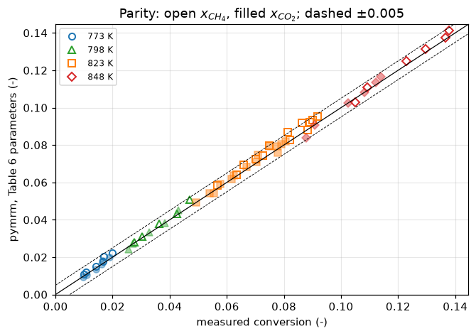
Both equilibrium intercepts, invisible to check 2, fail every deviation claim here. A transposed digit in an adsorption preexponential (K_CO, K_H2) is not caught by the measurements; it is caught by check 1, which is why the round trip has to be sharp enough to see it.
The activity factors quoted in Reuse are exercised here, not validated. The runs they belong to (the paper’s Figures 4 and 5, and fresh catalyst) are different chemistry that this page does not model. The rate coefficients multiplied by each factor are run against these data, the reference-level runs, so the fit can only get worse.
ACT = {}
for f, what in ((1.225, "the paper's Figures 4 and 5"), (2.246, "fresh catalyst")):
    ACT[f] = data_metrics(deviations(solve_all(replace(kin, activity=f))))["mad_conversion"]
    print(f"   k1, k2, k3 x {f:5.3f} ({what:28s}): MAD against this page's data {ACT[f]:.5f}")
    claims.value(f"mad_activity_{f:.3f}".replace(".", "p"), ACT[f],
                 note="exercised, not validated: these data are the reference-level runs")
_k1 = replace(kin, eq=(a1, b1 + 1, a2, b2))
for f in ACT:
    brk(DATA_CASES[0][0], f"mad_activity_{f:.3f}".replace(".", "p"),
        data_metrics(deviations(solve_all(replace(_k1, activity=f))))["mad_conversion"])
k1, k2, k3 x 1.225 (the paper's Figures 4 and 5 ): MAD against this page's data 0.00628
k1, k2, k3 x 2.246 (fresh catalyst ): MAD against this page's data 0.01695What pymrm adds
The paper draws four curves through its points and stops. Two questions it leaves open can be answered by running the model rather than reading it.
None of this needs pymrm as such: the same two ODEs integrate with solve_ivp, and check 4 does exactly that. What the pymrm form buys is reuse (see Reuse).
Where does the residual come from? The deviation is not uniform: the bias in methane conversion grows with space time.
print("bias in x_CH4, by space time (all four temperatures)")
for i, (lo, hi) in enumerate(BINS):
    n = int(((obs.quantity == "x_CH4") & (obs.W_F >= lo) & (obs.W_F < hi)).sum())
    print(f"   W/F {lo:.2f}-{hi:.2f}:  n = {n:2d}   bias = {DM[f'bias_x_ch4_bin{i + 1}']:+.5f}")
print(f"   short over long: {DM['bias_short_over_long']:.2f}")

# How far from equilibrium is the gas? beta_i = Q_i / K_i: 1 at equilibrium, where
# the rate of reaction i vanishes.
print("\napproach to equilibrium at 848 K (beta = Q/K; 1 = equilibrated)")
RS = {T: reference_solution(kin, T, TAU_MAX, P_T, SR, HR) for T in TEMPS}


def beta_ref(k, sol, T, tau):
    """beta_I, beta_II, beta_III on the Radau dense solution ``sol`` at space time ``tau``."""
    x = sol(tau)
    return np.array(k.beta(x[0], x[1], T, P_T, SR, HR))


for tau in (0.13, 0.20, 0.28, 0.35):
    b = beta_ref(kin, RS[848.0], 848.0, tau)
    print(f"   tau = {tau:.2f}:  I {b[0]:.3f}   II {b[1]:.3f}   III {b[2]:.3f}")
b = beta_ref(kin, RS[848.0], 848.0, TAU_MAX)
print(f"   outlet {TAU_MAX:.2f}:  I {b[0]:.3f}   II {b[1]:.3f}   III {b[2]:.3f}")


def beta_long(ms, k):
    """beta_I and beta_III at every measured x_CH4 point with W/F >= LONG."""
    s = obs[(obs.quantity == "x_CH4") & (obs.W_F >= LONG)]
    return np.array([ms[r.temperature_K].beta(r.W_F) for r in s.itertuples()])


BL = beta_long(models, kin)
print(f"\nat the measured points with W/F >= {LONG}: beta_I {BL[:, 0].min():.2f} to "
      f"{BL[:, 0].max():.2f}, beta_III {BL[:, 2].min():.2f} to {BL[:, 2].max():.2f}")
claims.value("beta_I_long_min", BL[:, 0].min())
claims.value("beta_I_long_max", BL[:, 0].max())
claims.value("beta_III_long_min", BL[:, 2].min())
claims.value("beta_III_long_max", BL[:, 2].max())
_bl = beta_long(CASE_MODELS[DATA_CASES[0][0]], DATA_CASES[0][1])
for j, name in ((0, "beta_I_long"), (2, "beta_III_long")):
    brk(DATA_CASES[0][0], f"{name}_min", _bl[:, j].min())
    brk(DATA_CASES[0][0], f"{name}_max", _bl[:, j].max())

# Sensitivity: K1, K2 and K3 each multiplied by 0.95 and 1.05, at the same
# measured long-space-time points the bias is taken over, on the same grid.
def k_halfspan(k, shift=0.05):
    out = {}
    for T in TEMPS:
        s = obs[(obs.quantity == "x_CH4") & (obs.W_F >= LONG) & (obs.temperature_K == T)]
        lo, hi = (SteamReformer(replace(k, eq_factor=f), T, P_T, SR, HR, TAU_MAX, N_TAU)
                  .solve().at(s.W_F.to_numpy(), 0) for f in (1 - shift, 1 + shift))
        out[T] = float(np.mean(np.abs(hi - lo)) / 2)
    return out


HS = k_halfspan(kin)
print(f"\nsensitivity of x_CH4 to a 5 % shift in every K_i, at the measured points with "
      f"W/F >= {LONG}, against the bias there")
for T in TEMPS:
    n = int(((obs.quantity == "x_CH4") & (obs.W_F >= LONG) & (obs.temperature_K == T)).sum())
    print(f"   {T:.0f} K (n = {n:2d}):  |half-span| {HS[T]:.4f}   observed bias "
          f"{DM[f'bias_long_{T:.0f}K']:+.4f}   ratio {HS[T] / DM[f'bias_long_{T:.0f}K']:.2f}")
    claims.value(f"k_halfspan_long_{T:.0f}K", HS[T])
RATIO = {T: HS[T] / DM[f"bias_long_{T:.0f}K"] for T in TEMPS}
for T in TEMPS:
    claims.value(f"k_halfspan_bias_ratio_{T:.0f}K", RATIO[T],
                 note="half-span of a 5 % shift in every K_i over the observed bias, W/F >= LONG")
# the wording below holds only while the hot pair is comparable and the cold pair is not
HOT, COLD = (823.0, 848.0), (773.0, 798.0)
claims.bound("k_halfspan_ratio_hot_min", min(RATIO[T] for T in HOT), min=0.5, basis="chosen",
             note="'the same size' at 823 and 848 K: ratio within a factor of two of 1")
claims.bound("k_halfspan_ratio_hot_max", max(RATIO[T] for T in HOT), max=2.0, basis="chosen",
             note="'the same size' at 823 and 848 K: ratio within a factor of two of 1")
claims.bound("k_halfspan_ratio_cold_max", max(RATIO[T] for T in COLD), max=0.5, basis="chosen",
             note="at 773 and 798 K the shift is under half the bias, so the argument fails")
for lab, k in DATA_CASES[:2]:
    hb = k_halfspan(k)
    for T in TEMPS:
        brk(lab, f"k_halfspan_long_{T:.0f}K", hb[T])
    bb = data_metrics(deviations(CASE_MODELS[lab]))
    rb = {T: hb[T] / bb[f"bias_long_{T:.0f}K"] for T in TEMPS}
    for T in TEMPS:
        brk(lab, f"k_halfspan_bias_ratio_{T:.0f}K", rb[T])
    brk(lab, "k_halfspan_ratio_hot_min", min(rb[T] for T in HOT))
    brk(lab, "k_halfspan_ratio_hot_max", max(rb[T] for T in HOT))
    brk(lab, "k_halfspan_ratio_cold_max", max(rb[T] for T in COLD))
_h25 = k_halfspan(kin, 0.25)
brk("a 25 % shift in every K_i instead of 5 % (k_halfspan(k, shift=0.25))",
    "k_halfspan_ratio_hot_max", max(_h25[T] / DM[f"bias_long_{T:.0f}K"] for T in HOT))
brk("a 25 % shift in every K_i instead of 5 % (k_halfspan(k, shift=0.25))",
    "k_halfspan_ratio_cold_max", max(_h25[T] / DM[f"bias_long_{T:.0f}K"] for T in COLD))
bias in x_CH4, by space time (all four temperatures)
W/F 0.12-0.20: n = 11 bias = +0.00116
W/F 0.20-0.28: n = 8 bias = +0.00174
W/F 0.28-0.42: n = 11 bias = +0.00321
short over long: 0.36
approach to equilibrium at 848 K (beta = Q/K; 1 = equilibrated)
tau = 0.13: I 0.514 II 0.826 III 0.424
tau = 0.20: I 0.709 II 0.920 III 0.653
tau = 0.28: I 0.851 II 0.965 III 0.821
tau = 0.35: I 0.920 II 0.982 III 0.903
outlet 0.45: I 0.968 II 0.993 III 0.961
at the measured points with W/F >= 0.28: beta_I 0.57 to 0.90, beta_III 0.45 to 0.88
sensitivity of x_CH4 to a 5 % shift in every K_i, at the measured points with W/F >= 0.28, against the bias there
773 K (n = 2): |half-span| 0.0005 observed bias +0.0028 ratio 0.19
798 K (n = 1): |half-span| 0.0014 observed bias +0.0039 ratio 0.36
823 K (n = 6): |half-span| 0.0025 observed bias +0.0035 ratio 0.71
848 K (n = 2): |half-span| 0.0035 observed bias +0.0023 ratio 1.54display(Markdown(
f"A 5 % shift in the equilibrium constants moves the long-space-time predictions by "
f"{HS[823.0]:.4f} at 823 K and {HS[848.0]:.4f} at 848 K, against observed biases of "
f"{DM['bias_long_823K']:+.4f} and {DM['bias_long_848K']:+.4f} there (ratios "
f"{RATIO[823.0]:.2f} and {RATIO[848.0]:.2f}): the same size. Xu and Froment do not report "
f"the $K_i$ they used, so at those two temperatures the residual at long space time is "
f"inside the uncertainty of an ingredient the paper does not supply, and cannot be "
f"charged to the kinetics. **At 773 and 798 K that argument fails.** There the gas is further from "
f"equilibrium ($\\beta_\\mathrm{{I}}$ down to {BL[:, 0].min():.2f} at the measured points), "
f"the same shift moves the prediction by only {HS[773.0]:.4f} and {HS[798.0]:.4f}, "
f"{RATIO[773.0]:.2f} and {RATIO[798.0]:.2f} of the biases ({DM['bias_long_773K']:+.4f} and "
f"{DM['bias_long_798K']:+.4f}), and the equilibrium constants do not explain the residual. "
f"At short space time the bias is {DM['bias_short_over_long']:.2f} of its long-space-time "
f"value."))A 5 % shift in the equilibrium constants moves the long-space-time predictions by 0.0025 at 823 K and 0.0035 at 848 K, against observed biases of +0.0035 and +0.0023 there (ratios 0.71 and 1.54): the same size. Xu and Froment do not report the \(K_i\) they used, so at those two temperatures the residual at long space time is inside the uncertainty of an ingredient the paper does not supply, and cannot be charged to the kinetics. At 773 and 798 K that argument fails. There the gas is further from equilibrium (\(\beta_\mathrm{I}\) down to 0.57 at the measured points), the same shift moves the prediction by only 0.0005 and 0.0014, 0.19 and 0.36 of the biases (+0.0028 and +0.0039), and the equilibrium constants do not explain the residual. At short space time the bias is 0.36 of its long-space-time value.
Where does each reaction stop being kinetically controlled? The \(\beta\) values split the reactor into regimes: the water-gas shift equilibrates first and well before the reforming reactions do, which is the behaviour the paper asserts from its \(V(\mathrm{II})\) plot but never shows against space time. Below, the same thing across all four temperatures; the space time at which each reaction reaches \(\beta = 0.90\) is root-found on the Radau reference profile (dense output), so it carries no grid error.
fig, axes = plt.subplots(1, 2, figsize=(11.5, 4.2), sharey=True)
tau = np.linspace(0.005, TAU_MAX, 200)
for T in TEMPS:
    b = np.array(models[T].beta(tau)).T
    axes[0].plot(tau, b[:, 0], color=COL[T], lw=1.6, label=f"{T:.0f} K")
    axes[0].plot(tau, b[:, 2], color=COL[T], lw=1.0, ls=":")
    axes[1].plot(tau, b[:, 1], color=COL[T], lw=1.6, label=f"{T:.0f} K")
for ax, ttl in zip(axes, ["reforming: I (solid), III (dotted)", "water-gas shift: II"]):
    ax.axhline(1.0, color="k", lw=0.8)
    ax.axhline(0.90, color="k", lw=0.6, ls="--")
    ax.set(xlabel=r"$W/F^{0}_{\mathrm{CH_4}}$  (g$_\mathrm{cat}$ h / mol$_{\mathrm{CH_4}}$)",
           xlim=(0, TAU_MAX), ylim=(0, 1.05), title=ttl)
axes[0].set_ylabel(r"$\beta = Q/K$  (-), 1 = equilibrated")
axes[0].legend(fontsize=8, loc="lower right")
fig.suptitle("Where each reaction stops being kinetically controlled", fontsize=11)
fig.tight_layout()
plt.show()


def tau90(k, sol, T, i):
    """Space time at which beta_i reaches 0.90 on the Radau dense solution ``sol``;
    None if the bed ends first."""
    f = lambda t: beta_ref(k, sol, T, t)[i] - 0.90   # noqa: E731
    return brentq(f, models[T].tau_c[0], TAU_MAX, xtol=1e-12) if f(TAU_MAX) > 0 else None


def tau90_fv(m, i):
    """The same crossing root-found on the finite-volume profile of model ``m``."""
    f = lambda t: m.beta(t)[i] - 0.90   # noqa: E731
    return brentq(f, m.tau_c[0], TAU_MAX, xtol=1e-12) if f(TAU_MAX) > 0 else None


def beta_outlet(k, sol, T):
    return beta_ref(k, sol, T, TAU_MAX)


BO = {T: beta_outlet(kin, RS[T], T) for T in TEMPS}
N90 = claims.count("tau90_crossings_in_bed", [BO[T][i] for T in TEMPS for i in range(3)],
                   0.90, min_margin=0.005,
                   note="(T, reaction) pairs with beta > 0.90 at the outlet")
TAU90 = {(T, i): tau90(kin, RS[T], T, i) for T in TEMPS for i in range(3)}
print(f"space time (g_cat h/mol_CH4) at which beta reaches 0.90, and beta at the outlet "
      f"tau = {TAU_MAX}; {N90} of 12 crossings lie in the bed")
for T in TEMPS:
    hit = [f"{TAU90[T, i]:.3f}" if TAU90[T, i] is not None else ">0.45" for i in range(3)]
    print(f"   {T:.0f} K:  I {hit[0]:6s} II {hit[1]:6s} III {hit[2]:6s}  |  beta at the outlet "
          f"{BO[T][0]:.3f}, {BO[T][1]:.3f}, {BO[T][2]:.3f}   beta_II - beta_I {BO[T][1] - BO[T][0]:+.3f}")
for T in (823.0, 848.0):
    print(f"   {T:.0f} K: the shift reaches 0.90 at {TAU90[T, 1] / TAU90[T, 0]:.2f} of the space "
          "time reforming (I) needs")
GAP = [BO[T][1] - BO[T][0] for T in TEMPS]
claims.value("beta_gap_outlet_min", min(GAP))
claims.value("beta_gap_outlet_max", max(GAP))
for T in (823.0, 848.0):
    claims.value(f"tau90_ratio_II_I_{T:.0f}K", TAU90[T, 1] / TAU90[T, 0], rtol=1e-3)
for (T, i) in ((798.0, 1), (823.0, 0), (823.0, 1), (848.0, 0), (848.0, 1), (848.0, 2)):
    claims.value(f"tau90_{('I', 'II', 'III')[i]}_{T:.0f}K", TAU90[T, i], rtol=1e-3)

# The crossings above are root-found on the Radau profile; the finite-volume
# profile runs late by its first-order grid error. The largest gap, over the
# crossings that lie in the bed, is bounded by the grid error measured above.
CROSS = [(T, i) for (T, i) in TAU90 if TAU90[T, i] is not None]
FV_GAP = max(abs(tau90_fv(models[T], i) - TAU90[T, i]) for T, i in CROSS)
print(f"largest gap between the finite-volume ({N_TAU} cells) and the Radau crossing: {FV_GAP:.1e}")
claims.bound("beta90_fv_vs_radau_max", FV_GAP, max=1e-3, basis="theory",
             note="max over the in-bed crossings of |finite volumes - Radau|, first-order grid error")
_coarse = solve_all(kin, 100)
brk("a tenth of the cells (n_tau = 100), crossings root-found on the finite-volume profile",
    "beta90_fv_vs_radau_max",
    max(abs(tau90_fv(_coarse[T], i) - TAU90[T, i]) for T, i in CROSS))

_lab, _k = DATA_CASES[1]                 # the K2 intercept: the shift's equilibrium moves
_rs = {T: reference_solution(_k, T, TAU_MAX, P_T, SR, HR) for T in TEMPS}
_bo = {T: beta_outlet(_k, _rs[T], T) for T in TEMPS}
_gap = [_bo[T][1] - _bo[T][0] for T in TEMPS]
brk(_lab, "beta_gap_outlet_min", min(_gap))
brk(_lab, "beta_gap_outlet_max", max(_gap))
brk(_lab, "tau90_crossings_in_bed", int(sum(_bo[T][i] > 0.90 for T in TEMPS for i in range(3))))
for T in (823.0, 848.0):
    t2, t1 = tau90(_k, _rs[T], T, 1), tau90(_k, _rs[T], T, 0)
    brk(_lab, f"tau90_ratio_II_I_{T:.0f}K", np.nan if t2 is None or t1 is None else t2 / t1)
for (T, i) in ((798.0, 1), (823.0, 0), (823.0, 1), (848.0, 0), (848.0, 1), (848.0, 2)):
    t = tau90(_k, _rs[T], T, i)
    brk(_lab, f"tau90_{('I', 'II', 'III')[i]}_{T:.0f}K", np.nan if t is None else t)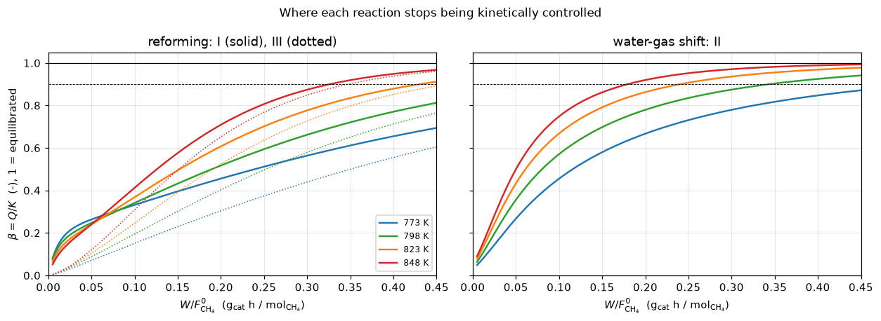
space time (g_cat h/mol_CH4) at which beta reaches 0.90, and beta at the outlet tau = 0.45; 6 of 12 crossings lie in the bed
   773 K:  I >0.45  II >0.45  III >0.45   |  beta at the outlet 0.694, 0.872, 0.605   beta_II - beta_I +0.177
   798 K:  I >0.45  II 0.343  III >0.45   |  beta at the outlet 0.813, 0.941, 0.765   beta_II - beta_I +0.129
   823 K:  I 0.430  II 0.240  III >0.45   |  beta at the outlet 0.912, 0.978, 0.892   beta_II - beta_I +0.066
   848 K:  I 0.326  II 0.179  III 0.346   |  beta at the outlet 0.968, 0.993, 0.961   beta_II - beta_I +0.025
   823 K: the shift reaches 0.90 at 0.56 of the space time reforming (I) needs
   848 K: the shift reaches 0.90 at 0.55 of the space time reforming (I) needs
largest gap between the finite-volume (1000 cells) and the Radau crossing: 4.9e-04
The break table
Every number above is registered as a claim; each row injects one defect through an argument or a parameter and reports what the claim becomes, and whether the claim’s own check catches it. A row that does not catch is kept when it shows a check’s blind spot (the intercepts in check 2, the adsorption preexponentials in check 5, the fourth-figure slip in check 1).
print(f"{'injected defect':<70} {'claim':<42} {'clean':>11} {'broken':>11}  caught")
for row, metric, clean, broken, caught in BREAK:
    if claims.metrics[metric]["kind"] == "bound":
        shown, br = f"(here {clean:.2g})", f"{float(broken):.3g}"
    else:
        shown, br = f"{float(clean):11.5g}", f"{float(broken):11.5g}"
    print(f"{row[:70]:<70} {metric[:42]:<42} {shown:>11} {br:>11}  {'yes' if caught else 'NO'}")
_caught = {mt for _, mt, _, _, c in BREAK if c}
_open = sorted(k for k in claims.metrics if k not in _caught and not claims.metrics[k].get("structural"))
_struct = sorted(k for k in claims.metrics if claims.metrics[k].get("structural"))
print(f"\n{len(BREAK)} rows; {len(_caught)} of {len(claims.metrics)} claims are failed by at least "
      f"one row; structural: {', '.join(_struct) or 'none'}; open: {', '.join(_open) or 'none'}")
injected defect claim clean broken caught
the bed outlet TAU_MAX read as the last measurement W_F_measured_max 0.4046 0.45 yes
regular expression matching the W/F error instead of the conversion er digitisation_error_conversion 0.0006 0.0007 yes
K_CO A 8.23e-5 -> 8.32e-5 (rows_with('K_CO', 'A', '8.32e-5')) param_round_trip_worst_pct 1.4432 1.4432 NO
K_CO A 8.23e-5 -> 8.32e-5 (rows_with('K_CO', 'A', '8.32e-5')) param_round_trip_worst_ratio_to_precision 2.3203 4.8973 yes
K_CO A 8.23e-5 -> 8.32e-5 (rows_with('K_CO', 'A', '8.32e-5')) param_round_trip_ratio_sum 10.438 13.67 yes
k3 A 1.020e15 -> 1.002e15 (rows_with('k3', 'A', '1.002e15')) param_round_trip_worst_pct 1.4432 1.2844 yes
k3 A 1.020e15 -> 1.002e15 (rows_with('k3', 'A', '1.002e15')) param_round_trip_worst_ratio_to_precision 2.3203 2.3203 NO
k3 A 1.020e15 -> 1.002e15 (rows_with('k3', 'A', '1.002e15')) param_round_trip_ratio_sum 10.438 9.3214 yes
K_H2O A 1.77e5 -> 1.71e5 (rows_with('K_H2O', 'A', '1.71e5')) param_round_trip_worst_pct 1.4432 3.2424 yes
K_H2O A 1.77e5 -> 1.71e5 (rows_with('K_H2O', 'A', '1.71e5')) param_round_trip_worst_ratio_to_precision 2.3203 8.5888 yes
K_H2O A 1.77e5 -> 1.71e5 (rows_with('K_H2O', 'A', '1.71e5')) param_round_trip_ratio_sum 10.438 18.326 yes
k2 A 1.955e6 -> 1.965e6 (rows_with('k2', 'A', '1.965e6')) param_round_trip_worst_pct 1.4432 1.4432 NO
k2 A 1.955e6 -> 1.965e6 (rows_with('k2', 'A', '1.965e6')) param_round_trip_worst_ratio_to_precision 2.3203 6.3864 yes
k2 A 1.955e6 -> 1.965e6 (rows_with('k2', 'A', '1.965e6')) param_round_trip_ratio_sum 10.438 14.504 yes
k1 A 4.225e15 -> 4.226e15 (rows_with('k1', 'A', '4.226e15')) param_round_trip_worst_pct 1.4432 1.4432 NO
k1 A 4.225e15 -> 4.226e15 (rows_with('k1', 'A', '4.226e15')) param_round_trip_worst_ratio_to_precision 2.3203 2.3203 NO
k1 A 4.225e15 -> 4.226e15 (rows_with('k1', 'A', '4.226e15')) param_round_trip_ratio_sum 10.438 10.462 NO
k1 E 240.1 -> 240.2 (rows_with('k1', 'E', '240.2')) param_round_trip_worst_pct 1.4432 1.4432 NO
k1 E 240.1 -> 240.2 (rows_with('k1', 'E', '240.2')) param_round_trip_worst_ratio_to_precision 2.3203 2.3203 NO
k1 E 240.1 -> 240.2 (rows_with('k1', 'E', '240.2')) param_round_trip_ratio_sum 10.438 9.6939 yes
K_CH4 val 0.1791 -> 0.1719 (rows_with('K_CH4', 'val', '0.1719')) param_round_trip_worst_pct 1.4432 3.8854 yes
K_CH4 val 0.1791 -> 0.1719 (rows_with('K_CH4', 'val', '0.1719')) param_round_trip_worst_ratio_to_precision 2.3203 21.908 yes
K_CH4 val 0.1791 -> 0.1719 (rows_with('K_CH4', 'val', '0.1719')) param_round_trip_ratio_sum 10.438 31.55 yes
k1 E 240.1 -> 241.1 (rows_with('k1', 'E', '241.1')) param_round_trip_worst_pct 1.4432 18.85 yes
k1 E 240.1 -> 241.1 (rows_with('k1', 'E', '241.1')) param_round_trip_worst_ratio_to_precision 2.3203 19.492 yes
k1 E 240.1 -> 241.1 (rows_with('k1', 'E', '241.1')) param_round_trip_ratio_sum 10.438 28.601 yes
k1 A 4.225e15 -> 4.225e14 (rows_with('k1', 'A', '4.225e14')) param_round_trip_worst_pct 1.4432 887.16 yes
k1 A 4.225e15 -> 4.225e14 (rows_with('k1', 'A', '4.225e14')) param_round_trip_worst_ratio_to_precision 2.3203 917.38 yes
k1 A 4.225e15 -> 4.225e14 (rows_with('k1', 'A', '4.225e14')) param_round_trip_ratio_sum 10.438 926.49 yes
K_CH4 T_ref 823.0 -> 648.0 (rows_with('K_CH4', 'T_ref', 648.0)) param_round_trip_worst_pct 1.4432 77.897 yes
K_CH4 T_ref 823.0 -> 648.0 (rows_with('K_CH4', 'T_ref', 648.0)) param_round_trip_worst_ratio_to_precision 2.3203 397.61 yes
K_CH4 T_ref 823.0 -> 648.0 (rows_with('K_CH4', 'T_ref', 648.0)) param_round_trip_ratio_sum 10.438 407.25 yes
k1 E printed as 240.10 (one more digit) e_precision_share_pct 0.92808 0.092808 yes
K_CH4 E -38.28 -> -38.82 (rows_with('K_CH4', 'E', '-38.82')) tref_slip_factor_K_CH4 0.22103 0.19995 yes
K_H2O E 88.68 -> 89.68 (rows_with('K_H2O', 'E', '89.68')) tref_slip_factor_K_H2O 33.033 39.771 yes
K1 slope a1 26830 -> 26380 (transposition) (XuFroment(eq=...)) equilibrium_vs_table7_worst_pct 1.926 2.5377 yes
K2 slope a2 4400 -> 4040 (transposition) (XuFroment(eq=...)) equilibrium_vs_table7_worst_pct 1.926 9.9502 yes
K1 intercept b1 30.114 -> 31.114 (K1 x e) (XuFroment(eq=...)) equilibrium_vs_table7_worst_pct 1.926 1.926 NO
K2 intercept b2 -4.036 -> -3.036 (K2 x e) (XuFroment(eq=...)) equilibrium_vs_table7_worst_pct 1.926 1.926 NO
H2 formed as 3 x_CH4, no x_CO2 term (stoich row H2 = (3, 0)) atom_balance_worst (here 2.2e-16) 0.266 yes
CO formed as x_CH4 - 2 x_CO2 (stoich row CO = (1, -2)) min_partial_pressure_rel (here 2.5e-06) 2.45e-06 NO
face read instead of centre read (at(..., read='face')) disc_error_max_n1000 4.1404e-05 0.00011175 yes
face read instead of centre read (at(..., read='face')) disc_error_share_of_mad_pct 2.4142 6.5158 yes
a quarter of the cells (n_tau = 250) disc_error_max_n1000 4.1404e-05 0.00016504 yes
a quarter of the cells (n_tau = 250) disc_error_share_of_mad_pct 2.4142 9.6228 yes
Radau reference at rtol 1e-5 (reference_profile(..., rtol=1e-5)) radau_reference_tolerance_gap (here 1.1e-12) 7.37e-08 yes
nearest cell value instead of interpolation (at(..., read='nearest')) grid_order_observed (here 1) 0.506 yes
ladder whose last rung is 4001 cells after 4000 grid_finest_over_roundoff (here 1.2e+07) 3.66e+03 yes
Newton stopped after one iteration (solve(maxfev=1, strict=False)) newton_backward_error_worst (here 1.3e-15) 0.000933 yes
K1 intercept b1 30.114 -> 31.114 (XuFroment(eq=...)) mad_conversion 0.0017151 0.016043 yes
K1 intercept b1 30.114 -> 31.114 (XuFroment(eq=...)) max_dev_conversion 0.005817 0.047213 yes
K1 intercept b1 30.114 -> 31.114 (XuFroment(eq=...)) bias_conversion 0.0012962 0.016043 yes
K1 intercept b1 30.114 -> 31.114 (XuFroment(eq=...)) mad_x_ch4 0.0022188 0.018748 yes
K1 intercept b1 30.114 -> 31.114 (XuFroment(eq=...)) mad_x_co2 0.0012276 0.013425 yes
K1 intercept b1 30.114 -> 31.114 (XuFroment(eq=...)) mad_rel_mean_pct 2.7301 25.537 yes
K1 intercept b1 30.114 -> 31.114 (XuFroment(eq=...)) bias_x_ch4_bin1 0.0011628 0.010767 yes
K1 intercept b1 30.114 -> 31.114 (XuFroment(eq=...)) bias_x_ch4_bin2 0.001736 0.016706 yes
K1 intercept b1 30.114 -> 31.114 (XuFroment(eq=...)) bias_x_ch4_bin3 0.0032074 0.028214 yes
K1 intercept b1 30.114 -> 31.114 (XuFroment(eq=...)) bias_short_over_long 0.36253 0.38161 yes
K1 intercept b1 30.114 -> 31.114 (XuFroment(eq=...)) bias_long_773K 0.0027918 0.0085104 yes
K1 intercept b1 30.114 -> 31.114 (XuFroment(eq=...)) bias_long_798K 0.0038698 0.019027 yes
K1 intercept b1 30.114 -> 31.114 (XuFroment(eq=...)) bias_long_823K 0.0035402 0.031405 yes
K1 intercept b1 30.114 -> 31.114 (XuFroment(eq=...)) bias_long_848K 0.0022932 0.042938 yes
K2 intercept b2 -4.036 -> -3.036 (XuFroment(eq=...)) mad_conversion 0.0017151 0.014787 yes
K2 intercept b2 -4.036 -> -3.036 (XuFroment(eq=...)) max_dev_conversion 0.005817 0.045476 yes
K2 intercept b2 -4.036 -> -3.036 (XuFroment(eq=...)) bias_conversion 0.0012962 0.014787 yes
K2 intercept b2 -4.036 -> -3.036 (XuFroment(eq=...)) mad_x_ch4 0.0022188 0.013662 yes
K2 intercept b2 -4.036 -> -3.036 (XuFroment(eq=...)) mad_x_co2 0.0012276 0.015876 yes
K2 intercept b2 -4.036 -> -3.036 (XuFroment(eq=...)) mad_rel_mean_pct 2.7301 23.539 yes
K2 intercept b2 -4.036 -> -3.036 (XuFroment(eq=...)) bias_x_ch4_bin1 0.0011628 0.0067588 yes
K2 intercept b2 -4.036 -> -3.036 (XuFroment(eq=...)) bias_x_ch4_bin2 0.001736 0.01182 yes
K2 intercept b2 -4.036 -> -3.036 (XuFroment(eq=...)) bias_x_ch4_bin3 0.0032074 0.021905 yes
K2 intercept b2 -4.036 -> -3.036 (XuFroment(eq=...)) bias_short_over_long 0.36253 0.30855 yes
K2 intercept b2 -4.036 -> -3.036 (XuFroment(eq=...)) bias_long_773K 0.0027918 0.0061777 yes
K2 intercept b2 -4.036 -> -3.036 (XuFroment(eq=...)) bias_long_798K 0.0038698 0.01464 yes
K2 intercept b2 -4.036 -> -3.036 (XuFroment(eq=...)) bias_long_823K 0.0035402 0.024677 yes
K2 intercept b2 -4.036 -> -3.036 (XuFroment(eq=...)) bias_long_848K 0.0022932 0.032948 yes
K_CO A 8.23e-05 -> 8.32e-05 (kin.edited('K_CO', A=8.32e-5)) mad_conversion 0.0017151 0.0017103 NO
K_CO A 8.23e-05 -> 8.32e-05 (kin.edited('K_CO', A=8.32e-5)) max_dev_conversion 0.005817 0.0058046 NO
K_CO A 8.23e-05 -> 8.32e-05 (kin.edited('K_CO', A=8.32e-5)) bias_conversion 0.0012962 0.0012865 NO
K_CO A 8.23e-05 -> 8.32e-05 (kin.edited('K_CO', A=8.32e-5)) mad_x_ch4 0.0022188 0.0022108 NO
K_CO A 8.23e-05 -> 8.32e-05 (kin.edited('K_CO', A=8.32e-5)) mad_x_co2 0.0012276 0.0012259 NO
K_CO A 8.23e-05 -> 8.32e-05 (kin.edited('K_CO', A=8.32e-5)) mad_rel_mean_pct 2.7301 2.7224 NO
K_CO A 8.23e-05 -> 8.32e-05 (kin.edited('K_CO', A=8.32e-5)) bias_x_ch4_bin1 0.0011628 0.001152 NO
K_CO A 8.23e-05 -> 8.32e-05 (kin.edited('K_CO', A=8.32e-5)) bias_x_ch4_bin2 0.001736 0.0017255 NO
K_CO A 8.23e-05 -> 8.32e-05 (kin.edited('K_CO', A=8.32e-5)) bias_x_ch4_bin3 0.0032074 0.0031977 NO
K_CO A 8.23e-05 -> 8.32e-05 (kin.edited('K_CO', A=8.32e-5)) bias_short_over_long 0.36253 0.36025 NO
K_CO A 8.23e-05 -> 8.32e-05 (kin.edited('K_CO', A=8.32e-5)) bias_long_773K 0.0027918 0.0027897 NO
K_CO A 8.23e-05 -> 8.32e-05 (kin.edited('K_CO', A=8.32e-5)) bias_long_798K 0.0038698 0.0038634 NO
K_CO A 8.23e-05 -> 8.32e-05 (kin.edited('K_CO', A=8.32e-5)) bias_long_823K 0.0035402 0.0035292 NO
K_CO A 8.23e-05 -> 8.32e-05 (kin.edited('K_CO', A=8.32e-5)) bias_long_848K 0.0022932 0.0022782 NO
k1 A 4.225e+15 -> 4.255e+15 (kin.edited('k1', A=4.255e15)) mad_conversion 0.0017151 0.0017809 NO
k1 A 4.225e+15 -> 4.255e+15 (kin.edited('k1', A=4.255e15)) max_dev_conversion 0.005817 0.0059506 NO
k1 A 4.225e+15 -> 4.255e+15 (kin.edited('k1', A=4.255e15)) bias_conversion 0.0012962 0.0014103 yes
k1 A 4.225e+15 -> 4.255e+15 (kin.edited('k1', A=4.255e15)) mad_x_ch4 0.0022188 0.002317 NO
k1 A 4.225e+15 -> 4.255e+15 (kin.edited('k1', A=4.255e15)) mad_x_co2 0.0012276 0.0012621 NO
k1 A 4.225e+15 -> 4.255e+15 (kin.edited('k1', A=4.255e15)) mad_rel_mean_pct 2.7301 2.8349 NO
k1 A 4.225e+15 -> 4.255e+15 (kin.edited('k1', A=4.255e15)) bias_x_ch4_bin1 0.0011628 0.0013087 yes
k1 A 4.225e+15 -> 4.255e+15 (kin.edited('k1', A=4.255e15)) bias_x_ch4_bin2 0.001736 0.0018601 yes
k1 A 4.225e+15 -> 4.255e+15 (kin.edited('k1', A=4.255e15)) bias_x_ch4_bin3 0.0032074 0.0033088 NO
k1 A 4.225e+15 -> 4.255e+15 (kin.edited('k1', A=4.255e15)) bias_short_over_long 0.36253 0.39554 yes
k1 A 4.225e+15 -> 4.255e+15 (kin.edited('k1', A=4.255e15)) bias_long_773K 0.0027918 0.002846 NO
k1 A 4.225e+15 -> 4.255e+15 (kin.edited('k1', A=4.255e15)) bias_long_798K 0.0038698 0.0039627 NO
k1 A 4.225e+15 -> 4.255e+15 (kin.edited('k1', A=4.255e15)) bias_long_823K 0.0035402 0.003652 NO
k1 A 4.225e+15 -> 4.255e+15 (kin.edited('k1', A=4.255e15)) bias_long_848K 0.0022932 0.002415 yes
k3 A 1.02e+15 -> 1.002e+15 (kin.edited('k3', A=1.002e15)) mad_conversion 0.0017151 0.0016629 NO
k3 A 1.02e+15 -> 1.002e+15 (kin.edited('k3', A=1.002e15)) max_dev_conversion 0.005817 0.0056851 NO
k3 A 1.02e+15 -> 1.002e+15 (kin.edited('k3', A=1.002e15)) bias_conversion 0.0012962 0.0011783 yes
k3 A 1.02e+15 -> 1.002e+15 (kin.edited('k3', A=1.002e15)) mad_x_ch4 0.0022188 0.0021191 NO
k3 A 1.02e+15 -> 1.002e+15 (kin.edited('k3', A=1.002e15)) mad_x_co2 0.0012276 0.0012214 NO
k3 A 1.02e+15 -> 1.002e+15 (kin.edited('k3', A=1.002e15)) mad_rel_mean_pct 2.7301 2.647 NO
k3 A 1.02e+15 -> 1.002e+15 (kin.edited('k3', A=1.002e15)) bias_x_ch4_bin1 0.0011628 0.001016 yes
k3 A 1.02e+15 -> 1.002e+15 (kin.edited('k3', A=1.002e15)) bias_x_ch4_bin2 0.001736 0.0016117 yes
k3 A 1.02e+15 -> 1.002e+15 (kin.edited('k3', A=1.002e15)) bias_x_ch4_bin3 0.0032074 0.0031069 NO
k3 A 1.02e+15 -> 1.002e+15 (kin.edited('k3', A=1.002e15)) bias_short_over_long 0.36253 0.32702 yes
k3 A 1.02e+15 -> 1.002e+15 (kin.edited('k3', A=1.002e15)) bias_long_773K 0.0027918 0.0027251 NO
k3 A 1.02e+15 -> 1.002e+15 (kin.edited('k3', A=1.002e15)) bias_long_798K 0.0038698 0.003767 NO
k3 A 1.02e+15 -> 1.002e+15 (kin.edited('k3', A=1.002e15)) bias_long_823K 0.0035402 0.0034305 NO
k3 A 1.02e+15 -> 1.002e+15 (kin.edited('k3', A=1.002e15)) bias_long_848K 0.0022932 0.0021881 NO
K_H2 A 6.12e-09 -> 6.21e-09 (kin.edited('K_H2', A=6.21e-9)) mad_conversion 0.0017151 0.0017145 NO
K_H2 A 6.12e-09 -> 6.21e-09 (kin.edited('K_H2', A=6.21e-9)) max_dev_conversion 0.005817 0.0058158 NO
K_H2 A 6.12e-09 -> 6.21e-09 (kin.edited('K_H2', A=6.21e-9)) bias_conversion 0.0012962 0.0012951 NO
K_H2 A 6.12e-09 -> 6.21e-09 (kin.edited('K_H2', A=6.21e-9)) mad_x_ch4 0.0022188 0.0022178 NO
K_H2 A 6.12e-09 -> 6.21e-09 (kin.edited('K_H2', A=6.21e-9)) mad_x_co2 0.0012276 0.0012274 NO
K_H2 A 6.12e-09 -> 6.21e-09 (kin.edited('K_H2', A=6.21e-9)) mad_rel_mean_pct 2.7301 2.7291 NO
K_H2 A 6.12e-09 -> 6.21e-09 (kin.edited('K_H2', A=6.21e-9)) bias_x_ch4_bin1 0.0011628 0.0011615 NO
K_H2 A 6.12e-09 -> 6.21e-09 (kin.edited('K_H2', A=6.21e-9)) bias_x_ch4_bin2 0.001736 0.0017347 NO
K_H2 A 6.12e-09 -> 6.21e-09 (kin.edited('K_H2', A=6.21e-9)) bias_x_ch4_bin3 0.0032074 0.0032063 NO
K_H2 A 6.12e-09 -> 6.21e-09 (kin.edited('K_H2', A=6.21e-9)) bias_short_over_long 0.36253 0.36225 NO
K_H2 A 6.12e-09 -> 6.21e-09 (kin.edited('K_H2', A=6.21e-9)) bias_long_773K 0.0027918 0.0027906 NO
K_H2 A 6.12e-09 -> 6.21e-09 (kin.edited('K_H2', A=6.21e-9)) bias_long_798K 0.0038698 0.0038684 NO
K_H2 A 6.12e-09 -> 6.21e-09 (kin.edited('K_H2', A=6.21e-9)) bias_long_823K 0.0035402 0.0035391 NO
K_H2 A 6.12e-09 -> 6.21e-09 (kin.edited('K_H2', A=6.21e-9)) bias_long_848K 0.0022932 0.0022925 NO
K1 intercept b1 30.114 -> 31.114 (XuFroment(eq=...)) mad_activity_1p225 0.006285 0.024632 yes
K1 intercept b1 30.114 -> 31.114 (XuFroment(eq=...)) mad_activity_2p246 0.016945 0.047305 yes
K1 intercept b1 30.114 -> 31.114 (XuFroment(eq=...)) beta_I_long_min 0.5694 0.29388 yes
K1 intercept b1 30.114 -> 31.114 (XuFroment(eq=...)) beta_I_long_max 0.90233 0.66074 yes
K1 intercept b1 30.114 -> 31.114 (XuFroment(eq=...)) beta_III_long_min 0.44654 0.21902 yes
K1 intercept b1 30.114 -> 31.114 (XuFroment(eq=...)) beta_III_long_max 0.88236 0.63338 yes
K1 intercept b1 30.114 -> 31.114 (XuFroment(eq=...)) k_halfspan_long_773K 0.00051695 0.0003062 yes
K1 intercept b1 30.114 -> 31.114 (XuFroment(eq=...)) k_halfspan_long_798K 0.0013962 0.00089574 yes
K1 intercept b1 30.114 -> 31.114 (XuFroment(eq=...)) k_halfspan_long_823K 0.0025059 0.0017527 yes
K1 intercept b1 30.114 -> 31.114 (XuFroment(eq=...)) k_halfspan_long_848K 0.0035392 0.0025887 yes
K1 intercept b1 30.114 -> 31.114 (XuFroment(eq=...)) k_halfspan_bias_ratio_773K 0.18517 0.03598 yes
K1 intercept b1 30.114 -> 31.114 (XuFroment(eq=...)) k_halfspan_bias_ratio_798K 0.36079 0.047078 yes
K1 intercept b1 30.114 -> 31.114 (XuFroment(eq=...)) k_halfspan_bias_ratio_823K 0.70784 0.05581 yes
K1 intercept b1 30.114 -> 31.114 (XuFroment(eq=...)) k_halfspan_bias_ratio_848K 1.5433 0.060289 yes
K1 intercept b1 30.114 -> 31.114 (XuFroment(eq=...)) k_halfspan_ratio_hot_min (here 0.71) 0.0558 yes
K1 intercept b1 30.114 -> 31.114 (XuFroment(eq=...)) k_halfspan_ratio_hot_max (here 1.5) 0.0603 NO
K1 intercept b1 30.114 -> 31.114 (XuFroment(eq=...)) k_halfspan_ratio_cold_max (here 0.36) 0.0471 NO
K2 intercept b2 -4.036 -> -3.036 (XuFroment(eq=...)) k_halfspan_long_773K 0.00051695 0.00035559 yes
K2 intercept b2 -4.036 -> -3.036 (XuFroment(eq=...)) k_halfspan_long_798K 0.0013962 0.00098196 yes
K2 intercept b2 -4.036 -> -3.036 (XuFroment(eq=...)) k_halfspan_long_823K 0.0025059 0.0019039 yes
K2 intercept b2 -4.036 -> -3.036 (XuFroment(eq=...)) k_halfspan_long_848K 0.0035392 0.0028712 yes
K2 intercept b2 -4.036 -> -3.036 (XuFroment(eq=...)) k_halfspan_bias_ratio_773K 0.18517 0.05756 yes
K2 intercept b2 -4.036 -> -3.036 (XuFroment(eq=...)) k_halfspan_bias_ratio_798K 0.36079 0.067076 yes
K2 intercept b2 -4.036 -> -3.036 (XuFroment(eq=...)) k_halfspan_bias_ratio_823K 0.70784 0.077154 yes
K2 intercept b2 -4.036 -> -3.036 (XuFroment(eq=...)) k_halfspan_bias_ratio_848K 1.5433 0.087142 yes
K2 intercept b2 -4.036 -> -3.036 (XuFroment(eq=...)) k_halfspan_ratio_hot_min (here 0.71) 0.0772 yes
K2 intercept b2 -4.036 -> -3.036 (XuFroment(eq=...)) k_halfspan_ratio_hot_max (here 1.5) 0.0871 NO
K2 intercept b2 -4.036 -> -3.036 (XuFroment(eq=...)) k_halfspan_ratio_cold_max (here 0.36) 0.0671 NO
a 25 % shift in every K_i instead of 5 % (k_halfspan(k, shift=0.25)) k_halfspan_ratio_hot_max (here 1.5) 7.86 yes
a 25 % shift in every K_i instead of 5 % (k_halfspan(k, shift=0.25)) k_halfspan_ratio_cold_max (here 0.36) 1.85 yes
a tenth of the cells (n_tau = 100), crossings root-found on the finite beta90_fv_vs_radau_max (here 0.00049) 0.00489 yes
K2 intercept b2 -4.036 -> -3.036 (XuFroment(eq=...)) beta_gap_outlet_min 0.025377 0.097067 yes
K2 intercept b2 -4.036 -> -3.036 (XuFroment(eq=...)) beta_gap_outlet_max 0.17713 0.20552 yes
K2 intercept b2 -4.036 -> -3.036 (XuFroment(eq=...)) tau90_crossings_in_bed 6 1 yes
K2 intercept b2 -4.036 -> -3.036 (XuFroment(eq=...)) tau90_ratio_II_I_823K 0.5587 nan yes
K2 intercept b2 -4.036 -> -3.036 (XuFroment(eq=...)) tau90_ratio_II_I_848K 0.55038 nan yes
K2 intercept b2 -4.036 -> -3.036 (XuFroment(eq=...)) tau90_II_798K 0.3431 nan yes
K2 intercept b2 -4.036 -> -3.036 (XuFroment(eq=...)) tau90_I_823K 0.42963 nan yes
K2 intercept b2 -4.036 -> -3.036 (XuFroment(eq=...)) tau90_II_823K 0.24003 nan yes
K2 intercept b2 -4.036 -> -3.036 (XuFroment(eq=...)) tau90_I_848K 0.32559 nan yes
K2 intercept b2 -4.036 -> -3.036 (XuFroment(eq=...)) tau90_II_848K 0.1792 0.33565 yes
K2 intercept b2 -4.036 -> -3.036 (XuFroment(eq=...)) tau90_III_848K 0.34647 nan yes
175 rows; 59 of 60 claims are failed by at least one row; structural: min_partial_pressure_rel; open: noneReuse
The kinetics on their own. XuFroment.rates(x_CH4, x_CO2, T, p_t, sr, hr) returns \(r_1, r_2, r_3\) in kmol/(kg\(_\mathrm{cat}\) h) and has no dependence on the reactor model. partial_pressures is the only piece tied to the single-feed parameterisation; swap it for a general mole-fraction vector and the rate equations carry over unchanged.
Three activity levels, and only one of them is tested here. Multiply \(k_1, k_2, k_3\) (XuFroment(activity=...)) by
- 1 for the steam-reforming reference level: what this page uses, what Tables 5 and 6 are, and the only level the measurements on this page belong to;
- 1.225 to reproduce the paper’s Figures 4 and 5 (reverse water-gas shift and methanation);
- 2.246 for fresh catalyst.
The last two are transcriptions from the paper’s text that nothing on this page validates. Check 5 executes them, so they are at least run, and shows what they do to the fit against these data, which is to make it worse, as it must. Reproducing Figures 4 and 5 would need the reverse water-gas shift and methanation feeds, which this page does not model. Treat both factors as unchecked.
The round trip is the check on the parameter reading, and it has a floor. Check 1 measures it: a slip smaller than a row’s own printed precision is invisible, and the worst per-row deviation cannot see anything smaller than the baseline scatter that the 0.1 kJ/mol precision of \(E\) already produces. If you re-read these tables from your own render, compare param_round_trip_ratio_sum, not the worst percentage.
The equilibrium constants are the weak ingredient. They are not from this paper, check 2 cannot see their intercepts, and at the two hotter temperatures the long-space-time residual is the size of a 5 % change in them. A model that replaces them by a thermodynamic database should re-run check 5.
Going further with the same residual. SteamReformer.residual is the whole model. To make the tube non-isothermal, add an enthalpy field to the state (a third entry on the last axis) and a wall-flux term; to resolve the pellet, keep this as the bulk equation and couple a B1.1-style intraparticle model to it, which is D1.4. First-order upwind is enough here because the error is checked at the points used (check 4); a profile with a sharp front would want ConvFluxTVD.
Related pages. B1.1 (intraparticle diffusion and reaction, the resistance these intrinsic kinetics deliberately exclude), D1.4 (fixed bed with resolved particles), C2.2, C2.6, D3.1.
Cite the source, not this page, for the kinetics: Xu, J. and Froment, G. F., Methane steam reforming, methanation and water-gas shift: I. Intrinsic kinetics, AIChE Journal 35(1) 88-96 (1989), doi:10.1002/aic.690350109.
# Prose numbers: each literal as written in the Markdown above, checked against its claim.
claims.says("0.93", "e_precision_share_pct")           # Validation intro, Reuse
claims.report();   # the semicolon keeps the notebook from echoing the payload
Claims for C2.1:
W_F_measured_max = 0.4046 value rtol 0.05
digitisation_error_conversion = 0.0006 value rtol 0.05
param_round_trip_worst_pct = 1.4432 value rtol 0.05
param_round_trip_worst_ratio_to_precision = 2.3203 value rtol 0.05
param_round_trip_ratio_sum = 10.438 value rtol 0.05
e_precision_share_pct = 0.92808 value rtol 0.05
tref_slip_factor_K_CH4 = 0.22103 value rtol 0.05
tref_slip_factor_K_H2O = 33.033 value rtol 0.05
equilibrium_vs_table7_worst_pct = 1.926 value rtol 0.05
atom_balance_worst = (here 2.2e-16) bound bound <= 1e-12 [identity]
min_partial_pressure_rel = (here 2.5e-06) bound bound >= 0 [theory]
disc_error_max_n1000 = 4.1404e-05 value rtol 0.05
disc_error_share_of_mad_pct = 2.4142 value rtol 0.05
radau_reference_tolerance_gap = (here 1.1e-12) bound bound <= 1e-08 [tolerance]
grid_order_observed = (here 1.0e+00) bound bound [0.95, 1.05] [theory]
grid_finest_over_roundoff = (here 1.2e+07) bound bound >= 10000 [theory]
newton_backward_error_worst = (here 1.3e-15) bound bound <= 1e-08 [tolerance]
mad_conversion = 0.0017151 value rtol 0.05
max_dev_conversion = 0.005817 value rtol 0.05
bias_conversion = 0.0012962 value rtol 0.05
mad_x_ch4 = 0.0022188 value rtol 0.05
mad_x_co2 = 0.0012276 value rtol 0.05
mad_rel_mean_pct = 2.7301 value rtol 0.05
bias_x_ch4_bin1 = 0.0011628 value rtol 0.05
bias_x_ch4_bin2 = 0.001736 value rtol 0.05
bias_x_ch4_bin3 = 0.0032074 value rtol 0.05
bias_short_over_long = 0.36253 value rtol 0.05
bias_long_773K = 0.0027918 value rtol 0.05
bias_long_798K = 0.0038698 value rtol 0.05
bias_long_823K = 0.0035402 value rtol 0.05
bias_long_848K = 0.0022932 value rtol 0.05
mad_activity_1p225 = 0.006285 value rtol 0.05
mad_activity_2p246 = 0.016945 value rtol 0.05
beta_I_long_min = 0.5694 value rtol 0.05
beta_I_long_max = 0.90233 value rtol 0.05
beta_III_long_min = 0.44654 value rtol 0.05
beta_III_long_max = 0.88236 value rtol 0.05
k_halfspan_long_773K = 0.00051695 value rtol 0.05
k_halfspan_long_798K = 0.0013962 value rtol 0.05
k_halfspan_long_823K = 0.0025059 value rtol 0.05
k_halfspan_long_848K = 0.0035392 value rtol 0.05
k_halfspan_bias_ratio_773K = 0.18517 value rtol 0.05
k_halfspan_bias_ratio_798K = 0.36079 value rtol 0.05
k_halfspan_bias_ratio_823K = 0.70784 value rtol 0.05
k_halfspan_bias_ratio_848K = 1.5433 value rtol 0.05
k_halfspan_ratio_hot_min = (here 7.1e-01) bound bound >= 0.5 [chosen]
k_halfspan_ratio_hot_max = (here 1.5e+00) bound bound <= 2 [chosen]
k_halfspan_ratio_cold_max = (here 3.6e-01) bound bound <= 0.5 [chosen]
tau90_crossings_in_bed = 6 exact exact, margin 0.00876
beta_gap_outlet_min = 0.025377 value rtol 0.05
beta_gap_outlet_max = 0.17713 value rtol 0.05
tau90_ratio_II_I_823K = 0.5587 value rtol 0.001
tau90_ratio_II_I_848K = 0.55038 value rtol 0.001
tau90_II_798K = 0.3431 value rtol 0.001
tau90_I_823K = 0.42963 value rtol 0.001
tau90_II_823K = 0.24003 value rtol 0.001
tau90_I_848K = 0.32559 value rtol 0.001
tau90_II_848K = 0.1792 value rtol 0.001
tau90_III_848K = 0.34647 value rtol 0.001
beta90_fv_vs_radau_max = (here 4.9e-04) bound bound <= 0.001 [theory]