# Bootstrap: the pymrm this page was checked with, and the gallery files it was
# published with. Works in a checkout, in CI and on a fresh Colab VM.
GALLERY_REF = "gallery-2026.11.10.3"  # replaced by the release tag at publication
PYMRM = ">=3.3.0,<4"  # equals meta.yaml pymrm_min_version, up to the next major
PAGE = "C1.3-mars-van-krevelen-redox"  # equals the page directory

import os, sys, urllib.request
from pathlib import Path
_shared = next((p / "shared" for p in (Path.cwd(), *Path.cwd().parents)
                if (p / "shared" / "gallery_bootstrap.py").is_file()), None)
if _shared is None:
    _shared = (Path(os.environ.get("XDG_CACHE_HOME") or Path.home() / ".cache")
               / "pymrm-gallery" / GALLERY_REF)
    _shared.mkdir(parents=True, exist_ok=True)
    urllib.request.urlretrieve(
        "https://raw.githubusercontent.com/computational-chemical-engineering/"
        f"pymrm-gallery/{GALLERY_REF}/shared/gallery_bootstrap.py",
        _shared / "gallery_bootstrap.py")
sys.path.insert(0, str(_shared))
sys.modules.pop("gallery_bootstrap", None)
from gallery_bootstrap import setup
setup(PAGE, PYMRM, GALLERY_REF); # the semicolon stops the cell echoing the pathMars-van Krevelen: the redox rate law, read from the paper that derived it
sec:C
struct:S1
tier:T0
data:tier2
phase:gas-solid
The 1954 origin of redox (Mars-van Krevelen) kinetics prints no rate constant for any aromatic oxidation; its printed numbers are all in the SO2 application. This page transcribes those tables at native resolution, reproduces the authors’ own k’ columns and their 23:77 converter catalyst split from printed inputs alone, ranks their integrated rate form against two period competitors on the data they reprinted, and proves two printed equations wrong from the paper’s own neighbouring equations.
Mars-van Krevelen: the redox rate law, read from the paper that derived it
Catalog ID: C1.3 · Structures: S1 (1D steady plug flow) · Tier: T0
Every partial-oxidation kinetics paper that writes
\[\dot n_R=\frac{1}{\dfrac{1}{k_1\,p_R}+\dfrac{\beta}{k_2\,p_{\mathrm{O}_2}^{\,n}}}\]
cites Mars and van Krevelen (1954). This page is about what that paper actually contains, which turns out to be different from what is usually attributed to it, and about the one complete worked calculation it prints: the design of a two-stage SO\(_2\) converter from the redox rate law, ending in a catalyst split the authors state as 23 : 77 against an actual plant’s 27 : 73. That calculation is reproduced here end to end from printed inputs alone, twice (adaptive quadrature and a pymrm plug-flow solve), and every printed intermediate on the way (two k\('\) tables, an activation energy, an equilibrium correlation, a gas-composition table) is recomputed and reconciled.
# Imports. The page's model.py is put on sys.path by setup().
import warnings
from fractions import Fraction

import numpy as np
import pandas as pd
import matplotlib.pyplot as plt
from IPython.display import Markdown, display
from scipy.integrate import IntegrationWarning, quad
from pymrm.checks import observed_orders
from gallery_utils import Claims, cite_data, load_data, load_meta
from model import (CAL, PAR, R_GAS, OptimumCurve, OptimumProfileConverter, alpha_eq,
                   f14, fit_block, fit_kuster, fit_neumann, fit_nu, kprime_pred,
                   oxygen_from_so2, split_quad)

plt.rcParams.update({"figure.dpi": 110, "axes.grid": True, "grid.alpha": 0.3})
claims = Claims(PAGE.split("-")[0])
EPS = np.finfo(float).eps
BREAK = []   # (injected defect, claim, clean value, broken value, caught)


def brk(row, metric, broken):
    """One injected defect: ``broken`` is what claim ``metric`` becomes with it."""
    caught = claims.breaks(row, metric, broken)
    BREAK.append((row, metric, claims[metric], broken, caught))


def brk_all(row, out, names=None):
    """Record a row for every claim in ``out`` (a section's results) that the defect moves."""
    for k in (out if names is None else names):
        if not k.startswith("_") and out[k] != claims[k]:   # a claim the defect reaches
            brk(row, k, out[k])
Background
What the paper is
Mars, P. and van Krevelen, D. W., Oxidations carried out by means of vanadium oxide catalysts, Special Supplement to Chemical Engineering Science 3 (1954) 41-59, doi:10.1016/S0009-2509(54)80005-4, a conference paper (Conference on Oxidation Processes) from the Staatsmijnen in Limburg Central Laboratory, Geleen, with a printed discussion by J. M. Smith, H. Jockush, H. A. Cheney, C. P. van Dijk, C. F. P. Bevington and G. C. A. Schuit. Everything on this page was read from cropped renders of the 19-page scan at its native 300 ppi (pdfimages -list reports CCITT-G4 bilevel at 300×300); the OCR text layer was used for nothing numeric.
The paper has three parts:
- Fluid-bed oxidation of aromatics (benzene, toluene, naphthalene, anthracene) over V\(_2\)O\(_5\), in a fluid bed because these oxidations are so exothermic that no fixed bed holds a uniform temperature. Both partial pressures influence the rate; the two-step redox scheme is proposed and the composite rate law derived (their eqs. 1-7).
- SO\(_2\) oxidation: the same formalism applied to three literature data sets (Küster 1904, Neumann 1928, Krichevskaya 1947), with the equilibrium term added and internal diffusion analysed (eqs. 8-16).
- A technical converter examined: rate constants derived from plant data (their Table 3), the optimum temperature curve computed, and the catalyst split between the two converters calculated and compared with practice.
What the paper prints, and what it does not
This matters, because the paper is cited far more often than read. Every number the paper prints is in the SO\(_2\) part. For the aromatic oxidations, the ones the mechanism is named for, the paper prints figures only (its Figs. 2-10): no table of rates, and no numeric value of \(k_1\), \(k_2\) or \(\beta\) for any aromatic, at any temperature. The only aromatic-side numbers in prose are the activation energy of the re-oxidation step, 22 kcal/mol, and the catalyst compositions in two footnotes. Anyone quoting “the Mars-van Krevelen constants” for benzene oxidation is quoting a later fit, not this paper.
Two more things commonly attributed to the paper deserve care:
- “Lattice oxygen” is a supposition here, not a demonstration. The authors attribute catalytic action to “certain oxygen ions” of the V\(_2\)O\(_5\) structure (their Fig. 5, after Byström et al.) and support the redox picture with colour changes and tetravalent-vanadium analyses from the literature. The rate-law derivation itself needs only a surface fraction \(\theta\) covered by oxygen; no isotope evidence exists in 1954.
- The authors themselves disclaim mechanistic proof. In the printed discussion, J. M. Smith observes that an adsorption-based three-step mechanism “leads to a kinetic equation similar to the one proposed”, and the authors reply: “Naturally, agreement between a kinetic formula and experimental data is not a proof of the correctness of the assumed reaction mechanism.” The same reply continues that agreement “may be held to support the assumed mechanism”: the disclaimer is about proof, not support. The famous rate form is kinetically indistinguishable from other two-step steady-state schemes, and the origin paper says so on its own last pages.
Why the SO₂ part carries the page
The printed tables are real measurements, Küster’s and Neumann’s, reprinted with the authors’ own derived k\('\) columns beside them, and the converter calculation is a complete worked design with printed inputs (Table 3), a printed equilibrium correlation (eq. 8) and a printed result (23 : 77). That is validation of the strongest kind available for a 1954 paper: printed intermediates that can be recomputed and compared, with no figure digitised.
The published model
The redox scheme and the composite rate law
The two reactions, exactly as formulated on journal page 46:
I. aromatic compound + oxidized catalyst \(\rightarrow\) oxidation products + reduced catalyst II. reduced catalyst + oxygen \(\rightarrow\) oxidized catalyst
With \(\theta\) the fraction of surface covered by oxygen, first order in the aromatic and order \(n\) in oxygen:
\[\dot n_R = k_1\,p_R\,\theta \tag{1}\] \[\dot n_{\mathrm{O}_2} = k_2\,p_{\mathrm{O}_2}^{\,n}\,(1-\theta) \tag{2}\] \[\dot n_R = \tfrac{1}{\beta}\,\dot n_{\mathrm{O}_2} \tag{3}\]
where \(\beta\) is the number of O\(_2\) molecules needed per molecule of aromatic converted, determined from the measured product distribution, not fitted. The steady state \(\beta k_1 p_R \theta = k_2 p_{\mathrm{O}_2}^n (1-\theta)\) (their eq. 4) gives eq. (5) for \(\theta\) and the composite law, their boxed eq. (6):
\[\dot n_R=\frac{1}{\dfrac{1}{k_1\,p_R}+\dfrac{\beta}{k_2\,p_{\mathrm{O}_2}^{\,n}}} \tag{6}\]
Two resistances in series, reduction and re-oxidation. For the experimental test they integrate it over the (integrating, not stirred) fluid bed for \(n = 1\), their eq. (7):
\[\frac{1}{V_s}=\frac{1}{k_1}\ln\frac{(p_R)_0}{(p_R)_{\mathrm{final}}} +\frac{1}{k_2}\ln\frac{(p_{\mathrm{O}_2})_0}{(p_{\mathrm{O}_2})_{\mathrm{final}}}, \qquad (p_{\mathrm{O}_2})_{\mathrm{final}}=(p_{\mathrm{O}_2})_0-\beta\left[(p_R)_0-(p_R)_{\mathrm{final}}\right]\]
with \(V_s\) the space velocity. Eq. (7) is the exact integral of eq. (6) at \(n=1\) under \(\mathrm{d}p_{\mathrm{O}_2} = \beta\,\mathrm{d}p_R\). Figures 6-8 test this against their own benzene, naphthalene and anthracene runs: figures only, so they are outside this page’s scope (see The data).
The SO₂ chain
For SO\(_2\) the product retards the rate, so a third surface reaction and its equilibrium enter (\(K^\ast\) small), and with re-oxidation rate-determining the chain runs (journal page 50): equilibrium eq. (8),
\[K=\frac{p_{\mathrm{SO}_3}^2}{p_{\mathrm{SO}_2}^2\,p_{\mathrm{O}_2}}\ \ \text{(atm)},\qquad {}^{10}\!\log K=\frac{9880}{T}-9.34 \tag{8}\]
through \(\theta\) (eq. 10), the rate (eqs. 11-12), the high-conversion approximation (eq. 13), its conversion form (13a)
\[\dot n_{\mathrm{SO}_2}= k\,p_{\mathrm{O}_2}^{\,n}\, \frac{\alpha_{\mathrm{eq}}-\alpha}{\alpha\,\alpha_{\mathrm{eq}}} =\frac{k\,p_{\mathrm{O}_2}^{\,n}}{\alpha_{\mathrm{eq}}}\,\frac{1-\alpha'}{\alpha'} , \qquad \alpha'=\frac{\alpha}{\alpha_{\mathrm{eq}}} \tag{13a}\]
and its integrated form (14), which is what the k\('\) columns of Tables 1 and 2 were computed with:
\[\frac{k}{V_s}\,\frac{(\bar p_{\mathrm{O}_2})^n}{(p_{\mathrm{SO}_2})_0} =\alpha_{\mathrm{eq}}\left\{\ln\frac{1}{1-\alpha'}-\alpha'\right\} \tag{14}\]
For the technical catalyst, internal diffusion cuts in; the pore analysis gives the diffusion-limited rate (15) and its integral (16):
\[\dot n_{\mathrm{SO}_2}\sim r_p\sqrt{k\,D\,r_p\,(\bar p_{\mathrm{O}_2})^n\,(p_{\mathrm{SO}_2})_0\,\alpha'}\; \frac{1-\alpha'}{\alpha'} \tag{15}\]
\[\frac{k^\ast}{2}\sqrt{\frac{(p_{\mathrm{O}_2})^n}{(p_{\mathrm{SO}_2})_0}}\cdot\frac{t}{\alpha_{\mathrm{eq}}} =\sqrt{\alpha/\alpha_{\mathrm{eq}}}-\tanh^{-1}\sqrt{\alpha/\alpha_{\mathrm{eq}}} \tag{16 as printed}\]
Two printed equations the paper’s own neighbours contradict
Both are provable without leaving the paper, from its own results, with the alternatives printed.
Eq. (16): the right-hand side is sign-inverted. As printed, the RHS \(\sqrt{\alpha'}-\tanh^{-1}\sqrt{\alpha'}\) is \(\le 0\) for every \(\alpha'\) (since \(\tanh^{-1}x \ge x\)), while the LHS is a positive time. Integrating the paper’s own eq. (15), \(\alpha_{\mathrm{eq}}\,\mathrm{d}\alpha'/\mathrm{d}t \propto (1-\alpha')/\sqrt{\alpha'}\), so \(\int\!\sqrt{\alpha'}/(1-\alpha')\, \mathrm{d}\alpha' = 2\left[\tanh^{-1}\sqrt{\alpha'}-\sqrt{\alpha'}\right]\), reproduces the printed LHS exactly, prefactor and \(\alpha_{\mathrm{eq}}\) included, with the two RHS terms transposed. The check below does the integral numerically and scores both signs.
Eqs. (13a) and (14) disagree by one factor of \(\alpha_{\mathrm{eq}}\). Under the natural reading (\(\dot n_{\mathrm{SO}_2}=(p_{\mathrm{SO}_2})_0\, \mathrm{d}\alpha/\mathrm{d}t\), \(t = 1/V_s\)), integrating (13a) gives \(k'/V_s=\alpha_{\mathrm{eq}}^{\,2}\{\ln\frac{1}{1-\alpha'}-\alpha'\}\); the printed (14) carries \(\alpha_{\mathrm{eq}}\) to the first power. One of the two carries a typographical slip. The k\('\) recomputation below is run both ways and reports both, with the size of the stray factor at the conditions of Table 2; nothing downstream on this page depends on which the authors intended.
Also checked here: the van ’t Hoff slope of eq. (8) is a reaction enthalpy the paper states independently, “SO\(_2\) + ½O\(_2\) \(\rightarrow\) SO\(_3\) + 23 k.cal/mol” (journal page 48).
# Eq. (16): the numeric integral of eq. (15) against the printed and the corrected RHS.
APV = np.array([0.3, 0.7, 0.95])      # three values of alpha' at which the forms are scored
EQ16_EPSREL = 1e-10                   # quad relative tolerance


def eq16_numeric(epsrel=EQ16_EPSREL):
    """int_0^a' sqrt(x)/(1 - x) dx by adaptive quadrature."""
    return np.array([quad(lambda x: np.sqrt(x) / (1.0 - x), 0.0, a, epsabs=0.0,
                          epsrel=epsrel)[0] for a in APV])


def eq16_rhs(order):
    """2[atanh(sqrt a') - sqrt a'] in the corrected order, 2[sqrt a' - atanh(sqrt a')] as printed."""
    d = np.arctanh(np.sqrt(APV)) - np.sqrt(APV)
    return 2.0 * d if order == "corrected" else -2.0 * d


def eq16_gap(order):
    return float(np.max(np.abs(eq16_numeric() - eq16_rhs(order))))


print(pd.DataFrame({"alpha_prime": APV, "numeric integral of (15)": eq16_numeric(),
                    "2[atanh(sqrt a') - sqrt a'] (corrected)": eq16_rhs("corrected"),
                    "2[sqrt a' - atanh(sqrt a')] (as printed)": eq16_rhs("printed")})
      .to_string(index=False))
claims.bound("eq16_corrected_max_residual", eq16_gap("corrected"), max=1e-9, basis="tolerance",
             note="quad epsrel 1e-10 on integrals of size up to 2.4")
claims.value("eq16_printed_rhs_max_error", eq16_gap("printed"))
print(f"\nthe corrected RHS matches the numeric integral to below 1e-9 (here "
      f"{claims['eq16_corrected_max_residual']:.0e}); the printed RHS is wrong by up to "
      f"{claims['eq16_printed_rhs_max_error']:.3f}, and negative where the LHS is a positive time.")
brk("eq. (16) RHS as printed (terms transposed)", "eq16_corrected_max_residual",
    eq16_gap("printed"))
brk("eq. (16) RHS in the corrected order", "eq16_printed_rhs_max_error", eq16_gap("corrected"))


# The van 't Hoff slope of eq. (8) against the printed reaction heat. K is written
# for 2 SO2 + O2 -> 2 SO3, so the enthalpy per mol SO3 is half the slope.
def vant_hoff(par):
    dH = R_GAS * par["slope"] * np.log(10.0) / 2.0 / CAL
    return {"vantHoff_dH_kcal_per_mol_SO3": dH, "vantHoff_vs_printed_23": abs(dH / 23.0 - 1.0)}


VH = vant_hoff(PAR)
claims.value("vantHoff_dH_kcal_per_mol_SO3", VH["vantHoff_dH_kcal_per_mol_SO3"], unit="kcal/mol")
claims.value("vantHoff_vs_printed_23", VH["vantHoff_vs_printed_23"])
print(f"van 't Hoff slope of eq (8): dH = -{VH['vantHoff_dH_kcal_per_mol_SO3']:.2f} kcal/mol SO3 "
      f"against the printed 23 kcal/mol, {VH['vantHoff_vs_printed_23'] * 100:.1f} % apart.")
alpha_prime numeric integral of (15) 2[atanh(sqrt a') - sqrt a'] (corrected) 2[sqrt a' - atanh(sqrt a')] (as printed)
0.30 0.134799 0.134799 -0.134799
0.70 0.746550 0.746550 -0.746550
0.95 2.407186 2.407186 -2.407186
the corrected RHS matches the numeric integral to below 1e-9 (here 4e-16); the printed RHS is wrong by up to 4.814, and negative where the LHS is a positive time.
van 't Hoff slope of eq (8): dH = -22.60 kcal/mol SO3 against the printed 23 kcal/mol, 1.7 % apart.Parameters and assumptions
Everything printed that this page consumes, and the assumptions it has to add. Every printed constant sits in the dictionary PAR of model.py, which every function takes; the tables are read from the CSVs.
| quantity | value | status |
|---|---|---|
| equilibrium correlation | \(^{10}\!\log K = 9880/T - 9.34\) (atm, \(T\) in K) | printed, eq. (8) |
| technical-catalyst rate group \(k^\ast\sqrt{(\bar p_{\mathrm{O}_2})^n (p_{\mathrm{SO}_2})_0}\) | at 445 °C and 570 °C | printed, Table 3 |
| oxygen order for SO\(_2\) | \(n = \tfrac12\) (Krichevskaya’s data, Figs. 12-13; eq. 12 used with \(n = 0.5\)) | printed statement |
| converter targets | converter 1: 0 → 81 %; converter 2: 81 → 97 % | printed, journal page 55 |
| re-oxidation activation energy (no diffusion) | 22 kcal/mol | printed, journal page 47 |
| feed gas for the converter calculation | the 8 % SO\(_2\) row of Table 4 | assumed: the paper does not state the plant’s feed; every other Table 4 row is computed below |
| Neumann’s gas composition | SO\(_2\) + air, SO\(_2\) fraction fitted | not printed anywhere |
| Neumann’s velocity units | unknown; absorbed into one fitted scale | not printed anywhere |
| O\(_2\) content of air | 20.9 % | standard value, used for Neumann’s gas and Table 4’s burner gas |
Fit versus test, declared up front. Fitted on this page: (i) the global scale \(C\) and the SO\(_2\) inlet fraction \(s\) of the Neumann recomputation, fitted only on the 325-465 °C blocks; (ii) both parameters of the Küster recomputation (no test possible, Küster’s conditions are unprinted); (iii) one rate constant per temperature block in the rate-law discrimination; (iv) one stoichiometric coefficient in the Table 4 gas-composition question. Everything else is a test: the 475-550 °C Neumann blocks (nothing refitted), the activation energy against “about 9 kcal/mol”, the van ’t Hoff slope against 23 kcal/mol, and the catalyst split against 23 : 77, the last with no fitted quantity anywhere in its chain.
# The paper's own numbers that the page compares with (text, not tables).
PAPER = {"split_pct": 23.0,      # converter 1 share of catalyst, journal page 55
         "plant_split_pct": 27.0,  # the actual plant, same page
         "E_app_about": 9.0,     # kcal/mol, "proved to be about 9 kcal/mol"
         "E_reox": 22.0}         # kcal/mol, re-oxidation without diffusion, journal page 47
print({k: v for k, v in PAR.items()})
{'slope': 9880.0, 'intercept': 9.34, 'x_o2_air': 0.209, 'ap_power': 0.5, 'E_fac': 1.0, 'alpha_mid': 0.81, 'alpha_end': 0.97, 'T_lo': 450.0, 'T_hi': 1400.0, 'T_cap': None, 'boreskov_power': 0.8}The data
Four datasets, all transcribed from cropped renders at the scan’s native 300 ppi. Tables 1 and 2 are experimental measurements, but not the authors’ own: they are Küster’s (1904) and Neumann’s (1928), reprinted by Mars & van Krevelen with the authors’ own computed k\('\) columns beside them. The originals were not consulted (origin_not_consulted in the sidecars); every value is as this paper prints it, which is exactly what a page about this paper’s calculation needs.
Scoped out: everything that exists only as a figure. The aromatic-side kinetics (Figs. 2-3 conversion curves, Figs. 6-8 linearised fits, Fig. 9 Arrhenius, Fig. 10 Porter-catalyst comparison), Krichevskaya’s SO\(_2\) data (Figs. 12-13), Calderbank’s (Fig. 14), the plant temperature profile (Fig. 11) and the optimum-temperature curve (Fig. 16) are all figure-only. No figure is digitised and no number on this page is read from one. The cost is stated where it bites: the famous rate law’s own quantitative fit to the aromatic data is untested here because the paper prints no table to test it against, the strongest attribution finding on this page. What remains testable is everything the paper prints as numbers, which is the whole SO\(_2\) application.
NAMES = ["mars-vankrevelen-1954-table1-kuster", "mars-vankrevelen-1954-table2-neumann",
         "mars-vankrevelen-1954-table3-converter", "mars-vankrevelen-1954-table4-gas"]
t1, t2, t3, t4 = (load_data(n + ".csv", page=PAGE) for n in NAMES)
t2s = load_data(NAMES[1] + ".csv", page=PAGE, dtype=str)   # the printed digits, for the checksum
for name in NAMES:
    print(cite_data(load_meta(name + ".csv", page=PAGE)))
print(f"\nTable 1: {len(t1)} rows   Table 2: {len(t2)} rows ({int(t2.bracketed.sum())} bracketed)   "
      f"Table 3: {len(t3)} rows   Table 4: {len(t4)} rows")
FIT_ROWS = t2.temperature_C <= 465                       # the blocks the Neumann fit sees
TEST_ROWS = (t2.temperature_C >= 475) & (t2.bracketed == 0)
claims.exact("neumann_fit_rows", int(FIT_ROWS.sum()), structural=True,
             note="row count of the 325-465 C blocks in the CSV")
claims.exact("neumann_test_rows", int(TEST_ROWS.sum()), structural=True,
             note="unbracketed row count of the 475-550 C blocks in the CSV")
claims.exact("discrimination_rows", int((t2.bracketed == 0).sum()), structural=True,
             note="unbracketed rows of Table 2")
print(f"Neumann fit rows {claims['neumann_fit_rows']}, held-out test rows "
      f"{claims['neumann_test_rows']}, unbracketed rows {claims['discrimination_rows']}")


def slip(table, col, value, **where):
    """A copy of ``table`` with ``col`` set to ``value`` on the row matching ``where``."""
    out = table.copy()
    mask = np.logical_and.reduce([out[k] == v for k, v in where.items()])
    assert mask.sum() == 1, where
    out.loc[mask, col] = value
    return out
Mars, P.; van Krevelen, D. W. (1954) — Special Supplement to Chemical Engineering Science 3, 41-59 — doi:10.1016/S0009-2509(54)80005-4 — table
Mars, P.; van Krevelen, D. W. (1954) — Special Supplement to Chemical Engineering Science 3, 41-59 — doi:10.1016/S0009-2509(54)80005-4 — table
Mars, P.; van Krevelen, D. W. (1954) — Special Supplement to Chemical Engineering Science 3, 41-59 — doi:10.1016/S0009-2509(54)80005-4 — table
Mars, P.; van Krevelen, D. W. (1954) — Special Supplement to Chemical Engineering Science 3, 41-59 — doi:10.1016/S0009-2509(54)80005-4 — table
Table 1: 6 rows Table 2: 33 rows (1 bracketed) Table 3: 2 rows Table 4: 7 rows
Neumann fit rows 19, held-out test rows 13, unbracketed rows 32The paper’s own checksum: the printed k′ averages
Table 2 prints, per temperature block, the average of its unbracketed k\('\) values. The rows are printed to three decimals, so the mean of the printed rows can be compared with the printed average exactly, in units of the last digit: within half a unit is the same number rounded; up to one unit is what averaging rows that were themselves rounded allows; more is an arithmetic slip. The arithmetic below is exact (fractions of the printed digits).
def kavg_section(t2s):
    """Mean of each block's unbracketed printed k' against its printed average, exactly."""
    rows, out = [], {}
    for T, blk in t2s.groupby("temperature_C", sort=False):
        ok = blk[blk.bracketed == "0"]
        vals = [Fraction(v) for v in ok.k_prime]
        mean = sum(vals) / len(vals)
        printed = Fraction(blk.k_prime_avg_printed.iloc[0])
        units = abs(mean - printed) / Fraction(1, 1000)
        rows.append((int(T), mean, printed, units, vals))
    d = {T: u for T, _, _, u, _ in rows}
    out["kavg_checksum_worst_block"] = float(max(d.values()) / 1000)
    out["kavg_blocks_within_half_unit"] = sum(u < Fraction(1, 2) for u in d.values())
    out["kavg_blocks_rounding_tie"] = sum(u == Fraction(1, 2) for u in d.values())
    out["kavg_blocks_within_one_unit"] = sum(Fraction(1, 2) < u <= 1 for u in d.values())
    out["kavg_blocks_beyond_one_unit"] = sum(u > 1 for u in d.values())
    v425 = next(r for r in rows if r[0] == 425)
    out["_425"] = v425
    out["kavg_425_three_row_mean_is_printed"] = bool(sum(v425[4][:3]) / 3 == v425[2])
    out["_rows"] = rows
    return out


KAVG = kavg_section(t2s)
print("k' average: mean of the unbracketed printed rows against the printed average")
for T, mean, printed, units, _ in KAVG["_rows"]:
    print(f"  {T:3d} C: mean = {float(mean):.5f}   printed = {float(printed):.3f}   "
          f"difference {float(units):.2f} units of the last digit")
claims.value("kavg_checksum_worst_block", KAVG["kavg_checksum_worst_block"])
for k in ("kavg_blocks_within_half_unit", "kavg_blocks_rounding_tie",
          "kavg_blocks_within_one_unit", "kavg_blocks_beyond_one_unit",
          "kavg_425_three_row_mean_is_printed"):
    claims.exact(k, KAVG[k], note="exact rational arithmetic on the printed digits")
_tie = [T for T, _, _, u, _ in KAVG["_rows"] if u == Fraction(1, 2)]
_one = [T for T, _, _, u, _ in KAVG["_rows"] if Fraction(1, 2) < u <= 1]
_far = [(T, float(u)) for T, _, _, u, _ in KAVG["_rows"] if u > 1]
display(Markdown(
    f"{KAVG['kavg_blocks_within_half_unit']} blocks agree to the last printed digit. "
    f"{len(_tie)} ({', '.join(f'{T} °C' for T in _tie)}) is an exact rounding tie, half a unit. "
    f"{len(_one)} ({', '.join(f'{T} °C' for T in _one)}) differ by more than half a unit and at "
    "most one, which averaging rows already rounded to the last digit allows. "
    + " and ".join(f"{T} °C differs by {u:.2f} units" for T, u in _far)
    + ": the 425 °C block's four rows average "
    f"{float(KAVG['_425'][1]):.5f}, while its first three alone average exactly the printed "
    f"{float(KAVG['_425'][2]):.3f}, so the paper either mis-averaged or dropped its 750 row "
    "without saying so. The 475 °C gap is a second, smaller slip that rounding cannot explain. "
    "The column still works as a transcription checksum: a wrong digit in any row moves its "
    "block mean by more than these residues."))
k' average: mean of the unbracketed printed rows against the printed average
325 C: mean = 0.10733 printed = 0.107 difference 0.33 units of the last digit
375 C: mean = 0.18775 printed = 0.188 difference 0.25 units of the last digit
425 C: mean = 0.31125 printed = 0.315 difference 3.75 units of the last digit
450 C: mean = 0.36625 printed = 0.366 difference 0.25 units of the last digit
465 C: mean = 0.38975 printed = 0.389 difference 0.75 units of the last digit
475 C: mean = 0.41775 printed = 0.419 difference 1.25 units of the last digit
500 C: mean = 0.43650 printed = 0.436 difference 0.50 units of the last digit
525 C: mean = 0.50000 printed = 0.500 difference 0.00 units of the last digit
550 C: mean = 0.53600 printed = 0.535 difference 1.00 units of the last digit4 blocks agree to the last printed digit. 1 (500 °C) is an exact rounding tie, half a unit. 2 (465 °C, 550 °C) differ by more than half a unit and at most one, which averaging rows already rounded to the last digit allows. 425 °C differs by 3.75 units and 475 °C differs by 1.25 units: the 425 °C block’s four rows average 0.31125, while its first three alone average exactly the printed 0.315, so the paper either mis-averaged or dropped its 750 row without saying so. The 475 °C gap is a second, smaller slip that rounding cannot explain. The column still works as a transcription checksum: a wrong digit in any row moves its block mean by more than these residues.
Table 4: the printed arithmetic, and which gas the pairs are
Table 4 prints seven (%O\(_2\), %SO\(_2\)) feed pairs with two derived columns, \(\sqrt{\%\mathrm{O}_2\,\%\mathrm{SO}_2}\) (the optimum-space-velocity group for \(n = 1\)) and \(\sqrt{\sqrt{\%\mathrm{O}_2}\,\%\mathrm{SO}_2}\) (\(n = 1/2\)), and says “a weak maximum is found at 8 % SO\(_2\) and 11 % SO\(_2\), respectively”. The paper names both sulphur burning and pyrite roasting but never says which generated the pairs. Burning sulphur or pyrite in air with \(\nu\) mol O\(_2\) consumed per mol SO\(_2\) formed gives \(\%\mathrm{O}_2 = 20.9 - \%\mathrm{SO}_2\,(0.209 + 0.791\,\nu)\), linear in \(\nu\), so its least-squares \(\nu\) is closed form.
def t4_section(t4, par=PAR, exps=(1.0, 0.5)):
    """Table 4: the printed groups recomputed, their row maxima, and the stoichiometry fit.

    ``exps`` are the O2 exponents of the two groups (``n = 1`` and ``n = 1/2``).
    """
    out = {}
    g1 = np.sqrt(t4.pct_O2 ** exps[0] * t4.pct_SO2)
    g2 = np.sqrt(t4.pct_O2 ** exps[1] * t4.pct_SO2)
    out["table4_arithmetic_max_abs_dev"] = float(max(np.abs(g1 - t4.sqrt_O2_SO2_printed).max(),
                                                     np.abs(g2 - t4.sqrt_sqrtO2_SO2_printed).max()))
    for name, g in (("table4_max_row_n1_pct_SO2", g1), ("table4_max_row_nhalf_pct_SO2", g2)):
        top = np.sort(g.to_numpy())[::-1]
        out[name] = int(t4.pct_SO2.iloc[int(np.argmax(g.to_numpy()))])   # the row's printed %SO2
        out["_margin_" + name] = float((top[0] - top[1]) / top[0])
    nu = fit_nu(t4.pct_O2, t4.pct_SO2, par)
    rms = {lab: float(np.sqrt(np.mean((t4.pct_O2 - oxygen_from_so2(t4.pct_SO2, v, par)) ** 2)))
           for lab, v in (("pyrite", 11.0 / 8.0), ("sulphur", 1.0))}
    out["table4_nu_bestfit"] = nu
    out["table4_rms_pyrite"] = rms["pyrite"]
    out["table4_rms_sulphur"] = rms["sulphur"]
    out["table4_sulphur_over_pyrite"] = rms["sulphur"] / rms["pyrite"]
    return out


T4 = t4_section(t4)
claims.bound("table4_arithmetic_max_abs_dev", T4["table4_arithmetic_max_abs_dev"], max=0.05,
             basis="theory", note="the printed groups have one decimal: half a unit is 0.05")
for k in ("table4_max_row_n1_pct_SO2", "table4_max_row_nhalf_pct_SO2"):
    claims.exact(k, T4[k], margin=T4["_margin_" + k], min_margin=1e-3,
                 note="the Table 4 row (by its %SO2) with the largest recomputed group; "
                      "margin: relative gap to the runner-up")
claims.value("table4_nu_bestfit", T4["table4_nu_bestfit"], rtol=1e-3,
             note="a fitted parameter, closed form: held to a tenth of a per cent")
for k in ("table4_rms_pyrite", "table4_rms_sulphur", "table4_sulphur_over_pyrite"):
    claims.value(k, T4[k])
print(f"Table 4 groups recomputed: max |deviation| from the printed values "
      f"{T4['table4_arithmetic_max_abs_dev']:.3f}, inside the half unit (0.05) of their one "
      "printed decimal.")
print(f"largest sqrt(%O2 %SO2) on the {T4['table4_max_row_n1_pct_SO2']} % SO2 row, largest "
      f"sqrt(sqrt(%O2) %SO2) on the {T4['table4_max_row_nhalf_pct_SO2']} % SO2 row: the paper's "
      "'weak maximum ... at 8 % SO2 and 11 % SO2' is a maximum over its own printed rows.")
print(f"\nleast-squares O2-per-SO2 stoichiometry nu = {T4['table4_nu_bestfit']:.3f}")
print(f"pyrite roasting (4 FeS2 + 11 O2, nu = 11/8 = 1.375): rms = {T4['table4_rms_pyrite']:.3f} %-abs")
print(f"sulphur burning (S + O2, nu = 1):                    rms = {T4['table4_rms_sulphur']:.3f} %-abs")
print(f"The printed pairs are pyrite-roaster gas, by a factor "
      f"{T4['table4_sulphur_over_pyrite']:.0f} in rms. This attribution is an inference and is "
      "labelled so in the sidecar.")
Table 4 groups recomputed: max |deviation| from the printed values 0.049, inside the half unit (0.05) of their one printed decimal.
largest sqrt(%O2 %SO2) on the 8 % SO2 row, largest sqrt(sqrt(%O2) %SO2) on the 11 % SO2 row: the paper's 'weak maximum ... at 8 % SO2 and 11 % SO2' is a maximum over its own printed rows.
least-squares O2-per-SO2 stoichiometry nu = 1.386
pyrite roasting (4 FeS2 + 11 O2, nu = 11/8 = 1.375): rms = 0.130 %-abs
sulphur burning (S + O2, nu = 1): rms = 2.816 %-abs
The printed pairs are pyrite-roaster gas, by a factor 22 in rms. This attribution is an inference and is labelled so in the sidecar.Can the printed data discriminate the rate law?
The honest question for any composite rate law of this flexibility. Within a temperature block Neumann varied only the gas velocity, so composition dependence is invisible; what the data can test is the shape of \(\alpha(V_s)\), exactly where the MvK form differs from its period rivals. Three one-parameter-per-block laws, fitted per block by least squares in conversion, with \(\alpha_{\mathrm{eq}}\) from the fitted Neumann gas:
- MvK integrated, eq. (14): \(\alpha_{\mathrm{eq}}\{\ln\frac{1}{1-\alpha'}-\alpha'\}=k/V_s\), whose \(-\alpha'\) term is the SO\(_3\) retardation; solved for \(\alpha\) in closed form with the Lambert W function;
- plain first order to equilibrium: \(\alpha_{\mathrm{eq}}\ln\frac{1}{1-\alpha'}=k/V_s\), the same thing without retardation;
- Boreskov-Sokolova’s power law, printed on journal page 51: \(\mathrm{d}p_{\mathrm{SO}_3}/\mathrm{d}t = k\,p_{\mathrm{O}_2} (p_{\mathrm{SO}_2}/p_{\mathrm{SO}_3})^{0.8}\), with \(p_{\mathrm{O}_2}\) constant within a block, integrated in closed form (an incomplete beta function) and capped at \(\alpha_{\mathrm{eq}}\), since the law has no equilibrium term.
Each \(k\) is the root of the analytic derivative of the block’s sum of squares, found on a logarithmic scan from a hundredth of the block’s smallest velocity to thirty times its largest. A Langmuir-Hinshelwood form with an independent SO\(_3\) adsorption constant would add a second parameter per block and cannot be ranked fairly on 2-4 points per block; the comparison is confined to equal-parameter forms, and that is the stated scope of this discrimination.
LAWS = (("mvk", "MvK eq (14)"), ("first_order", "first order to equilibrium"),
        ("boreskov", "Boreskov 0.8 power law"))


def disc_section(t2, s, par=PAR, mvk_law="mvk", aeq_one=False, k_max=None):
    """Per-block rms (conversion points) of the three laws; ``mvk_law`` replaces the MvK form."""
    w = par["x_o2_air"] * (1.0 - s)
    per, edge, multi = {}, [], []
    for law, _ in LAWS:
        use = mvk_law if law == "mvk" else law
        per[law] = []
        for T, blk in t2.groupby("temperature_C"):
            aeq = 1.0 if aeq_one else alpha_eq(T + 273.15, s, w, par)
            f = fit_block(blk[blk.bracketed == 0], aeq, use, par, k_max)
            per[law].append(f["rms"])
            edge.append(f["at_edge"])
            multi.append(f["n_stationary"] > 1)
    out = {"discrimination_rms_mvk": float(np.mean(per["mvk"])),
           "discrimination_rms_first_order": float(np.mean(per["first_order"])),
           "discrimination_rms_boreskov": float(np.mean(per["boreskov"]))}
    out["discrimination_first_order_over_mvk"] = (out["discrimination_rms_first_order"]
                                                  / out["discrimination_rms_mvk"])
    out["discrimination_boreskov_over_mvk"] = (out["discrimination_rms_boreskov"]
                                               / out["discrimination_rms_mvk"])
    temps = sorted(t2.temperature_C.unique())
    b = np.array(per["boreskov"])
    order = np.argsort(b)[::-1]
    out["discrimination_boreskov_worst_block_C"] = int(temps[order[0]])
    out["_margin_worst"] = float((b[order[0]] - b[order[1]]) / b[order[0]])
    out["discrimination_fits_at_window_edge"] = int(sum(edge))
    out["discrimination_fits_with_several_stationary_points"] = int(sum(multi))
    out["_per"], out["_temps"] = per, temps
    return out


DISC = disc_section(t2, s_fit)
for law, lab in LAWS:
    print(f"{lab:28s}: per-block rms = {np.round(DISC['_per'][law], 2).tolist()} "
          f"(conversion points), mean {np.mean(DISC['_per'][law]):.2f}")
for k in ("discrimination_rms_mvk", "discrimination_rms_first_order",
          "discrimination_rms_boreskov", "discrimination_first_order_over_mvk",
          "discrimination_boreskov_over_mvk"):
    claims.value(k, DISC[k])
claims.exact("discrimination_boreskov_worst_block_C", DISC["discrimination_boreskov_worst_block_C"],
             margin=DISC["_margin_worst"], min_margin=0.01,
             note="block with the largest Boreskov rms; margin: relative gap to the runner-up")
claims.exact("discrimination_fits_at_window_edge", DISC["discrimination_fits_at_window_edge"],
             note="fits whose sum of squares still falls at the end of the k window")
claims.exact("discrimination_fits_with_several_stationary_points",
             DISC["discrimination_fits_with_several_stationary_points"],
             note="fits whose sum of squares has more than one stationary point in the window")
display(Markdown(
    f"On the {claims['discrimination_rows']} unbracketed conversions of Table 2 the eq. (14) "
    f"shape fits at {DISC['discrimination_rms_mvk']:.2f} points rms, Boreskov's 0.8-power law at "
    f"{DISC['discrimination_rms_boreskov']:.2f} (a factor "
    f"{DISC['discrimination_boreskov_over_mvk']:.1f}) and first order to equilibrium, the same "
    f"law without the retardation term, at {DISC['discrimination_rms_first_order']:.2f} (a factor "
    f"{DISC['discrimination_first_order_over_mvk']:.1f}). The retardation term earns its place. "
    f"Boreskov's law fails worst in the {DISC['discrimination_boreskov_worst_block_C']} °C block. "
    f"{DISC['discrimination_fits_at_window_edge']} of the "
    f"{3 * len(DISC['_temps'])} fits ends at the edge of its window and "
    f"{DISC['discrimination_fits_with_several_stationary_points']} has more than one stationary "
    "point: every rate constant is the one interior minimum of its block's sum of squares."))
MvK eq (14) : per-block rms = [1.95, 3.3, 0.72, 0.18, 0.36, 0.32, 1.04, 0.81, 0.41] (conversion points), mean 1.01
first order to equilibrium : per-block rms = [6.43, 3.61, 2.57, 2.32, 2.33, 2.16, 2.53, 2.21, 1.48] (conversion points), mean 2.85
Boreskov 0.8 power law : per-block rms = [3.3, 3.16, 1.68, 1.66, 2.02, 2.11, 2.91, 2.78, 2.62] (conversion points), mean 2.47On the 32 unbracketed conversions of Table 2 the eq. (14) shape fits at 1.01 points rms, Boreskov’s 0.8-power law at 2.47 (a factor 2.5) and first order to equilibrium, the same law without the retardation term, at 2.85 (a factor 2.8). The retardation term earns its place. Boreskov’s law fails worst in the 325 °C block. 0 of the 27 fits ends at the edge of its window and 0 has more than one stationary point: every rate constant is the one interior minimum of its block’s sum of squares.
PyMRM implementation: the converter calculation
The paper’s worked design (journal pages 53-55): along the optimum temperature curve (at every conversion, operate at the temperature that maximises the rate) compute the contact time, proportional to the catalyst amount, to go 0 → 81 % (converter 1) and 81 → 97 % (converter 2). The paper states the result as 23 : 77, against 27 : 73 in the actual plant.
The chain, every link printed: rate = eq. (15)’s diffusion-limited form \(A(T)\,(1-\alpha')/\sqrt{\alpha'}\) with the group \(A(T)=k^\ast\sqrt{(\bar p_{\mathrm{O}_2})^n (p_{\mathrm{SO}_2})_0}\) pinned by Table 3 at two temperatures and Arrhenius in between (that two-point line is the paper’s “apparent activation energy proved to be about 9 kcal/mol”); \(\alpha_{\mathrm{eq}}(T)\) from eq. (8); the feed of the 8 % SO\(_2\) row of Table 4. The optimum temperature at each conversion is the root of the analytic temperature derivative of \(\ln r\),
\[\frac{\partial \ln r}{\partial T} = \frac{E}{R T^2} + \left(\frac{1}{1-\alpha'}+\frac{1}{2\alpha'}\right)\alpha'\, \frac{\mathrm{d}\alpha_{\mathrm{eq}}/\mathrm{d}T}{\alpha_{\mathrm{eq}}} = 0 ,\]
on the window from 450 K to where \(\alpha_{\mathrm{eq}}(T) = \alpha\), with \(\alpha_{\mathrm{eq}}(T)\) a cubic spline through exact values; the rate on the curve is a cubic spline in \(\alpha\).
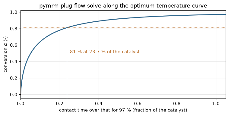
Two routes to the same integral. Route 1 is adaptive quadrature of \(\int\mathrm{d}\alpha/r\). Route 2 solves the plug-flow reactor with pymrm, \(\mathrm{d}\alpha/\mathrm{d}\tau = r(\alpha)\) as upwind convection at unit velocity plus a pointwise source, Newton on the assembled system, the C2.1 pattern; its split is the ratio of the contact times at which its own profile crosses 81 % and 97 %, each the root of the profile interpolated between face values. The two routes share the rate function \(r(\alpha)\) (and its splines), so their agreement tests the integration, not the rate law or its transcription; the break table injects those defects separately.
pymrm conventions used: operators assembled once; boundary conditions on the outward normal (inlet \(\alpha=0\) is {a:0, b:1, d:0} at the left face, a pure convective outlet {"outflow": True} at the right, read with compute_boundary_values); single-field layout (n, 1) so NumJac couples the field axis, not space; nu = 0 in construct_div, the flow coordinate being Cartesian.
FEED = t4[t4.pct_SO2 == 8].iloc[0]           # the Table 4 row used as the converter feed


def group_of(t3):
    """Table 3's two (T in K, rate group) pairs, lowest temperature first."""
    r = t3.sort_values("temperature_C")
    return tuple((float(T) + 273.15, float(A)) for T, A in
                 zip(r.temperature_C, r.kstar_group_atm_per_hr))


def design_section(t3, feed=FEED, par=PAR, n_alpha=350):
    """The design chain from printed inputs: E_app, the optimum curve and the quadrature split."""
    g = group_of(t3)
    (T1, A1), (T2, A2) = g
    E = np.log(A2 / A1) / (1.0 / T1 - 1.0 / T2) * R_GAS / CAL * par["E_fac"]
    s, w = feed.pct_SO2 / 100, feed.pct_O2 / 100
    curve = OptimumCurve(g, s, w, par, n_alpha=n_alpha)
    split, tau = split_quad(curve, par)
    out = {"Eapp_kcal_per_mol": E, "Eapp_vs_paper_about_9": abs(E / PAPER["E_app_about"] - 1.0),
           "ratio_22_over_Eapp": PAPER["E_reox"] / E,
           "split_converter1_pct_quad": split,
           "split_vs_paper_points": split - PAPER["split_pct"],
           "plant_minus_split_points": PAPER["plant_split_pct"] - split,
           "alpha_eq_570C_pyrite_gas": alpha_eq(T2, s, w, par)}
    for a in (0.40, 0.81, 0.90, 0.97):
        out[f"T_opt_{int(round(a * 100)):03d}_C"] = curve.T_opt(a) - 273.15
    out["optimum_curve_nodes_at_ceiling"] = curve.n_at_ceiling
    out["_curve"], out["_tau"] = curve, tau
    return out


DES = design_section(t3)
CURVE, TAU_TOTAL = DES["_curve"], DES["_tau"]
for k in ("Eapp_kcal_per_mol", "Eapp_vs_paper_about_9", "ratio_22_over_Eapp",
          "split_converter1_pct_quad", "split_vs_paper_points", "plant_minus_split_points",
          "alpha_eq_570C_pyrite_gas"):
    claims.value(k, DES[k])
for a in ("040", "081", "090", "097"):
    claims.value(f"T_opt_{a}_C", DES[f"T_opt_{a}_C"], rtol=2e-3, unit="degC")
claims.exact("optimum_curve_nodes_at_ceiling", DES["optimum_curve_nodes_at_ceiling"],
             note="conversion nodes whose optimum lands on the window's upper end")
print(f"apparent activation energy from Table 3's two rate groups: "
      f"E_app = {DES['Eapp_kcal_per_mol'] * CAL / 1000:.2f} kJ/mol = {DES['Eapp_kcal_per_mol']:.2f} kcal/mol")
print(f"  paper: 'the apparent activation energy proved to be about 9 kcal/mol': "
      f"{DES['Eapp_vs_paper_about_9'] * 100:.1f} % from 9")
print(f"  paper: 'the activation energy decreases by about a factor 2 if there is internal "
      f"diffusion': 22 / {DES['Eapp_kcal_per_mol']:.2f} = {DES['ratio_22_over_Eapp']:.2f}")
print(f"\nfeed: Table 4 row {FEED.pct_SO2:.0f} % SO2, {FEED.pct_O2:.1f} % O2. The optimum temperature "
      f"is interior at all {len(CURVE.a_nodes)} conversion nodes "
      f"({DES['optimum_curve_nodes_at_ceiling']} on the window's {PAR['T_hi']:.0f} K end).")
print(f"catalyst split along the optimum curve (quadrature): "
      f"{DES['split_converter1_pct_quad']:.1f} : {100 - DES['split_converter1_pct_quad']:.1f}   "
      f"[paper: 23 : 77, actual plant: 27 : 73]")
print(f"alpha_eq(570 C, this gas) = {DES['alpha_eq_570C_pyrite_gas']:.3f}: converter 1's 81 % target "
      "is essentially its equilibrium at its temperature level, the paper's own Fig. 11 story "
      "('converted rapidly but very incompletely owing to the unfavourable value of the "
      "equilibrium constant').")

# Numerics of the quadrature route, each against a second setting.
QUAD_TOL_GAP = abs(split_quad(CURVE, epsrel=1e-8)[0] - DES["split_converter1_pct_quad"])
_fine = OptimumCurve(group_of(t3), FEED.pct_SO2 / 100, FEED.pct_O2 / 100, n_T=2400, n_alpha=700)
INTERP_GAP = abs(split_quad(_fine)[0] - DES["split_converter1_pct_quad"])
SCALE_GAP = abs(split_quad(CURVE, scale=lambda a: 10.0)[0] - DES["split_converter1_pct_quad"])
claims.bound("split_quad_tolerance_gap", QUAD_TOL_GAP, max=1e-7, basis="tolerance",
             note="quad epsrel 1e-8 against 1e-10, split-points")
claims.bound("split_interpolant_gap", INTERP_GAP, max=1e-3, basis="chosen",
             note="splines on twice the nodes in T and in alpha; a thousandth of a "
                  "split-point is far below every comparison on the page")
claims.bound("split_scale_invariance_gap_points", SCALE_GAP, max=1e-9, basis="identity",
             note="every rate times 10: the split is a ratio of two integrals of 1/r")
print(f"quadrature at epsrel 1e-8 against 1e-10: below 1e-7 split-points (here {QUAD_TOL_GAP:.0e}); "
      f"splines on twice the nodes: below 1e-3 (here {INTERP_GAP:.0e}); every rate times 10: "
      f"below 1e-9 (here {SCALE_GAP:.0e}), the split is scale-invariant.")
apparent activation energy from Table 3's two rate groups: E_app = 35.91 kJ/mol = 8.58 kcal/mol
paper: 'the apparent activation energy proved to be about 9 kcal/mol': 4.6 % from 9
paper: 'the activation energy decreases by about a factor 2 if there is internal diffusion': 22 / 8.58 = 2.56
feed: Table 4 row 8 % SO2, 10.6 % O2. The optimum temperature is interior at all 350 conversion nodes (0 on the window's 1400 K end).
catalyst split along the optimum curve (quadrature): 23.6 : 76.4 [paper: 23 : 77, actual plant: 27 : 73]
alpha_eq(570 C, this gas) = 0.810: converter 1's 81 % target is essentially its equilibrium at its temperature level, the paper's own Fig. 11 story ('converted rapidly but very incompletely owing to the unfavourable value of the equilibrium constant').
quadrature at epsrel 1e-8 against 1e-10: below 1e-7 split-points (here 2e-10); splines on twice the nodes: below 1e-3 (here 2e-07); every rate times 10: below 1e-9 (here 1e-14), the split is scale-invariant.# The optimum-temperature curve (computed; Fig. 16 is figure-only and is not digitised).
al_plot = np.linspace(0.30, 0.969, 140)
T_plot = np.array([CURVE.T_opt(a) for a in al_plot]) - 273.15
aeq_T = np.linspace(430 + 273.15, 700 + 273.15, 200)
aeq_curve = [alpha_eq(T, FEED.pct_SO2 / 100, FEED.pct_O2 / 100) for T in aeq_T]
fig, ax = plt.subplots(1, 2, figsize=(10.5, 4.1))
ax[0].plot(al_plot, T_plot, color="#31688e", lw=2, label=r"computed $T_{\mathrm{opt}}(\alpha)$")
ax[0].plot(aeq_curve, aeq_T - 273.15, color="#888888", lw=1.4, ls="--",
label=r"equilibrium $\alpha_{\mathrm{eq}}(T)$")
for a in (PAR["alpha_mid"], PAR["alpha_end"]):
ax[0].axvline(a, color="#b5651d", lw=1, ls=":")
ax[0].set(xlabel=r"conversion $\alpha$ (-)", ylabel="temperature (°C)", ylim=(380, 660),
title="Optimum temperature against conversion\n(computed counterpart of the paper's Fig. 16)")
ax[0].legend(loc="lower left")
ax[1].semilogy(al_plot, 1.0 / CURVE.R(al_plot), color="#31688e", lw=2)
ax[1].axvline(PAR["alpha_mid"], color="#b5651d", lw=1, ls=":")
ax[1].set(xlabel=r"conversion $\alpha$ (-)", ylabel=r"catalyst demand $1/r$ (hr/atm)",
title="Where the catalyst goes:\n$1/r$ along the optimum curve")
fig.tight_layout()
plt.show()
display(Markdown(
f"The optimum temperature falls from {DES['T_opt_040_C']:.0f} °C at 40 % conversion to "
f"{DES['T_opt_081_C']:.0f} °C at 81 %, {DES['T_opt_090_C']:.0f} °C at 90 % and "
f"{DES['T_opt_097_C']:.0f} °C at 97 %: the first converter runs hot, near the 570 °C level "
"of Table 3, and the second ends well below its 445 °C level."))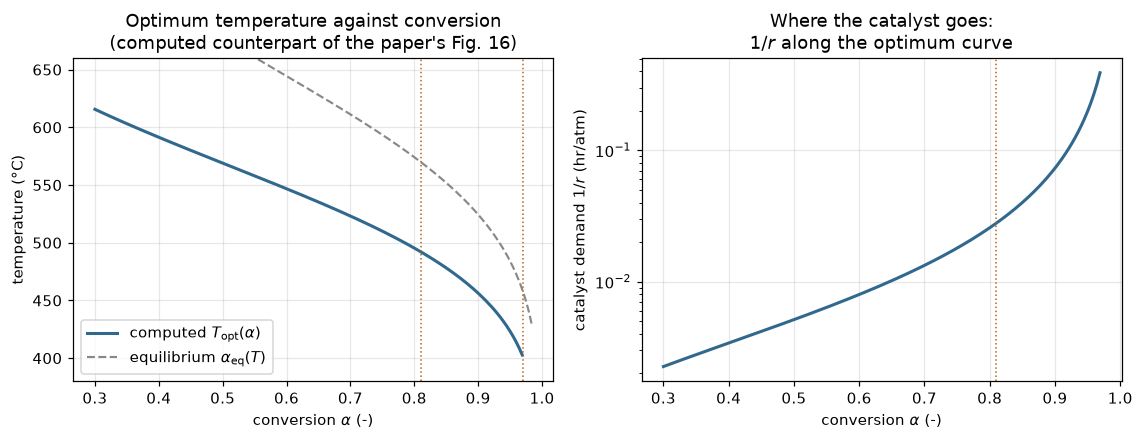
The optimum temperature falls from 591 °C at 40 % conversion to 492 °C at 81 %, 456 °C at 90 % and 401 °C at 97 %: the first converter runs hot, near the 570 °C level of Table 3, and the second ends well below its 445 °C level.
# Route 2: the pymrm plug-flow solve. The bed holds the 97 % crossing with room to spare.
BED = 1.05 * TAU_TOTAL
NS = (1000, 2000, 4000, 8000, 16000)
N_PAGE = 2000


def pymrm_split(R, n, bed=BED, read="face", maxfev=100, strict=True):
    """Converter-1 share (%) from the pymrm profile's own 81 % and 97 % crossings."""
    conv = OptimumProfileConverter(R, bed, n).solve(maxfev=maxfev, strict=strict)
    tau81 = conv.crossing(PAR["alpha_mid"], read)
    tau97 = conv.crossing(PAR["alpha_end"], read)
    return 100.0 * tau81 / tau97, conv


SPL, CONV = {}, {}
for n in (*NS, NS[-1] + 1):
    SPL[n], CONV[n] = pymrm_split(CURVE.R, n)
for n in NS:
    c = CONV[n]
    print(f"pymrm n = {n:5d}: newton converged in {c.result.nit} iterations, outlet alpha "
          f"(compute_boundary_values) {c.outlet():.5f}, split = {SPL[n]:.3f} : {100 - SPL[n]:.3f}")
OO = observed_orders(lambda n: SPL[n], NS)
FINEST = abs(SPL[NS[-1]] - SPL[NS[-2]])
GAP = abs(SPL[N_PAGE] - DES["split_converter1_pct_quad"])
BE_WORST = max(CONV[n].backward_error() for n in NS)
claims.value("split_converter1_pct_pymrm_n2000", SPL[N_PAGE])
claims.bound("split_routes_gap_points", GAP, max=0.15, basis="theory",
             note="first-order upwind on 2000 cells against the quadrature, split-points")
claims.bound("split_order_min", min(OO["orders"]), min=0.85, max=1.1, basis="theory",
             note="first-order upwind; successive differences, 1000 to 16000 cells")
claims.bound("split_order_spread", max(OO["orders"]) - min(OO["orders"]), max=0.05,
             basis="theory", note="the orders of a ladder in the asymptotic range agree")
claims.bound("split_finest_over_roundoff", FINEST / (NS[-1] * EPS), min=1e6, basis="theory",
             note="finest ladder change over n eps; the crossings are root-found to 1e-12")
claims.bound("newton_backward_error_worst", BE_WORST, max=1e-8, basis="tolerance",
             note="pymrm.checks.residual_check over the ladder; newton backward_tol 1e-8")


def floored_max_dev_from_one(floor):
    """Largest |order - 1| of the split ladder with the rate held at its value at ``floor`` below it."""
    oo = observed_orders(lambda n: pymrm_split(lambda u: CURVE.R(np.maximum(u, floor)), n)[0], NS)
    return float(np.max(np.abs(np.array(oo["orders"]) - 1.0))), oo["orders"]


FLOOR_DEV, FLOOR_ORDERS = floored_max_dev_from_one(0.2)
claims.bound("split_order_floored_max_dev_from_one", FLOOR_DEV, max=0.02, basis="theory",
             note="first-order upwind with r held at its alpha = 0.2 value below 0.2: orders near 1")
claims.bound("pymrm_outlet_beyond_target", CONV[N_PAGE].outlet() - PAR["alpha_end"], min=0.0,
             basis="chosen", note="the bed must hold the 97 % crossing")
print(f"\ndifference from the quadrature split: "
      + ", ".join(f"{abs(SPL[n] - DES['split_converter1_pct_quad']):.3f}" for n in NS)
      + f" split-points at n = {', '.join(map(str, NS))}")
print("observed orders from successive differences: " + ", ".join(f"{o:.3f}" for o in OO["orders"])
      + f"; finest change {FINEST:.1e} = {FINEST / (NS[-1] * EPS):.1e} times n eps")
print(f"Newton backward error below 1e-8 on every grid (here {BE_WORST:.0e})")
display(Markdown(
    f"On {N_PAGE} cells the pymrm route gives {SPL[N_PAGE]:.2f} : {100 - SPL[N_PAGE]:.2f}, "
    f"{GAP:.2f} split-points from the quadrature. The gap halves with each doubling of the grid, "
    f"at observed orders from {min(OO['orders']):.2f}, rising by {max(OO['orders']) - min(OO['orders']):.2f} "
    "over the ladder. With the rate held at its $\\alpha = 0.2$ value below 20 % conversion, which removes "
    "its $\\alpha^{-1/2}$ growth at the inlet, the orders lie within 0.02 of 1 "
    f"(here {FLOOR_DEV:.3f}). Both routes evaluate the same $r(\\alpha)$, so this "
    "agreement tests the integration only."))

fig, ax = plt.subplots(figsize=(7, 3.6))
c = CONV[N_PAGE]
tau81 = c.crossing(PAR["alpha_mid"])
tau97 = c.crossing(PAR["alpha_end"])
ax.plot(c.tau_f / tau97, np.concatenate([[0.0], c.alpha[:, 0]]), color="#31688e", lw=2)
ax.axhline(PAR["alpha_mid"], color="#b5651d", lw=1, ls=":")
ax.axvline(tau81 / tau97, color="#b5651d", lw=1, ls=":")
ax.annotate(f"  81 % at {SPL[N_PAGE]:.1f} % of the catalyst", (tau81 / tau97, 0.5), color="#b5651d")
ax.set(xlabel="contact time over that for 97 % (fraction of the catalyst)",
       ylabel=r"conversion $\alpha$ (-)", xlim=(0, 1.05),
       title="pymrm plug-flow solve along the optimum temperature curve")
fig.tight_layout()
plt.show()
pymrm n = 1000: newton converged in 7 iterations, outlet alpha (compute_boundary_values) 0.97219, split = 23.774 : 76.226
pymrm n = 2000: newton converged in 7 iterations, outlet alpha (compute_boundary_values) 0.97227, split = 23.702 : 76.298
pymrm n = 4000: newton converged in 7 iterations, outlet alpha (compute_boundary_values) 0.97232, split = 23.663 : 76.337
pymrm n = 8000: newton converged in 7 iterations, outlet alpha (compute_boundary_values) 0.97234, split = 23.642 : 76.358
pymrm n = 16000: newton converged in 7 iterations, outlet alpha (compute_boundary_values) 0.97235, split = 23.631 : 76.369
difference from the quadrature split: 0.155, 0.083, 0.044, 0.023, 0.012 split-points at n = 1000, 2000, 4000, 8000, 16000
observed orders from successive differences: 0.896, 0.908, 0.916; finest change 1.1e-02 = 3.1e+09 times n eps
Newton backward error below 1e-8 on every grid (here 2e-16)On 2000 cells the pymrm route gives 23.70 : 76.30, 0.08 split-points from the quadrature. The gap halves with each doubling of the grid, at observed orders from 0.90, rising by 0.02 over the ladder. With the rate held at its \(\alpha = 0.2\) value below 20 % conversion, which removes its \(\alpha^{-1/2}\) growth at the inlet, the orders lie within 0.02 of 1 (here 0.007). Both routes evaluate the same \(r(\alpha)\), so this agreement tests the integration only.
The feed the paper does not state
The plant’s feed is not printed, so the split is computed for every (%O\(_2\), %SO\(_2\)) pair of Table 4 that can reach the 97 % target at all: a feed reaches at most \(2\,\%\mathrm{O}_2/\%\mathrm{SO}_2\) of conversion before its oxygen runs out.
def feed_section(t3, t4, par=PAR):
    """The quadrature split for every Table 4 feed that can reach the converter target."""
    reach = 2.0 * t4.pct_O2 / t4.pct_SO2          # O2-limited conversion
    ok = reach > par["alpha_end"]
    out = {"feed_rows_reaching_target": int(ok.sum()),
           "_margin": float(np.min(np.abs(reach - par["alpha_end"])) / par["alpha_end"])}
    sp = {}
    for r in t4[ok].itertuples():
        sp[(r.pct_O2, r.pct_SO2)] = design_section(t3, r, par)["split_converter1_pct_quad"]
    out["feed_split_min_pct"] = min(sp.values())
    out["feed_split_max_pct"] = max(sp.values())
    out["feed_split_range_points"] = out["feed_split_max_pct"] - out["feed_split_min_pct"]
    out["_sp"], out["_reach"] = sp, reach
    return out


FEEDS = feed_section(t3, t4)
claims.exact("feed_rows_reaching_target", FEEDS["feed_rows_reaching_target"],
             margin=FEEDS["_margin"], min_margin=0.01,
             note="Table 4 rows with 2 %O2/%SO2 above the 97 % target; margin relative to it")
for k in ("feed_split_min_pct", "feed_split_max_pct", "feed_split_range_points"):
    claims.value(k, FEEDS[k])
for r in t4.itertuples():
    key = (r.pct_O2, r.pct_SO2)
    txt = (f"split {FEEDS['_sp'][key]:.2f}" if key in FEEDS["_sp"]
           else f"cannot reach 97 %: oxygen runs out at {FEEDS['_reach'][r.Index] * 100:.1f} %")
    print(f"  {r.pct_O2:4.1f} % O2, {r.pct_SO2:4.1f} % SO2: {txt}")
_bad = t4[FEEDS["_reach"] <= PAR["alpha_end"]].iloc[0]
display(Markdown(
    f"{FEEDS['feed_rows_reaching_target']} of the {len(t4)} printed feeds can reach 97 %; the "
    f"{_bad.pct_SO2:.0f} % SO$_2$ feed runs out of oxygen first. Over the others the split runs "
    f"from {FEEDS['feed_split_min_pct']:.2f} to {FEEDS['feed_split_max_pct']:.2f}, a range of "
    f"{FEEDS['feed_split_range_points']:.2f} split-points, against the paper's 23 : 77: the "
    "unstated plant feed does not undermine the reproduction."))
5.2 % O2, 12.0 % SO2: cannot reach 97 %: oxygen runs out at 86.7 %
6.6 % O2, 11.0 % SO2: split 22.47
7.8 % O2, 10.0 % SO2: split 23.24
9.0 % O2, 9.0 % SO2: split 23.48
10.6 % O2, 8.0 % SO2: split 23.62
11.9 % O2, 7.0 % SO2: split 23.69
13.0 % O2, 6.0 % SO2: split 23.736 of the 7 printed feeds can reach 97 %; the 12 % SO\(_2\) feed runs out of oxygen first. Over the others the split runs from 22.47 to 23.73, a range of 1.26 split-points, against the paper’s 23 : 77: the unstated plant feed does not undermine the reproduction.
Results
display(Markdown(f"""Read against the paper:

1. **The catalyst split reproduces.** From printed inputs only (Table 3's two
   rate groups, eq. (8), the 81 %/97 % targets, a printed Table 4 feed pair)
   the optimum-curve calculation gives **{DES['split_converter1_pct_quad']:.1f} :
   {100 - DES['split_converter1_pct_quad']:.1f}** against the paper's printed **23 : 77**,
   by two integration routes {GAP:.2f} split-points apart on {N_PAGE} cells. Nothing was
   fitted anywhere in that chain. The actual plant's 27 : 73 then sits
   {DES['plant_minus_split_points']:.1f} points from the optimum, which is the paper's own
   point: "the distribution of the catalyst is rather impervious to the temperature
   distribution."
2. **The printed intermediates hold up.** E$_{{\\mathrm{{app}}}}$ =
   {DES['Eapp_kcal_per_mol']:.2f} kcal/mol against "about 9"; the van 't Hoff slope of
   eq. (8) gives {VH['vantHoff_dH_kcal_per_mol_SO3']:.1f} kcal/mol against the printed 23; the
   k$'$ columns of both tables are reproduced to a few per cent, with the held-out
   475-550 °C blocks at {NEU['neumann_test_mean_dev'] * 100:.1f} % mean using eq. (14)
   exactly as printed.
3. **The rate law earns its shape on the reprinted data.** Equal-parameter
   discrimination puts eq. (14) at {DISC['discrimination_rms_mvk']:.2f} conversion-points
   rms against {DISC['discrimination_rms_boreskov']:.2f} for Boreskov's 0.8-power law and
   {DISC['discrimination_rms_first_order']:.2f} for first order to equilibrium: the
   retardation term is doing measurable work.
4. **Four printed defects found**, all provable from the paper itself: eq. (16)'s
   sign-inverted RHS; the $\\alpha_{{\\mathrm{{eq}}}}$-power mismatch between (13a) and
   (14); the 425 °C k$'$ average (0.315 printed, {float(KAVG['_425'][1]):.3f} computed, and
   0.315 is the mean of the block's first three rows); and Table 4's unstated
   stoichiometry settled as pyrite-roaster gas ($\\nu$ = {T4['table4_nu_bestfit']:.3f} fitted
   against 11/8 = 1.375, with sulphur burning excluded at {T4['table4_sulphur_over_pyrite']:.0f}
   times the rms).
5. **The one bracketed k$'$ is an outlier, not the row eq. (14) amplifies most**:
   {_n_more} unbracketed rows are more sensitive to a conversion error."""))
Read against the paper:
- The catalyst split reproduces. From printed inputs only (Table 3’s two rate groups, eq. (8), the 81 %/97 % targets, a printed Table 4 feed pair) the optimum-curve calculation gives 23.6 : 76.4 against the paper’s printed 23 : 77, by two integration routes 0.08 split-points apart on 2000 cells. Nothing was fitted anywhere in that chain. The actual plant’s 27 : 73 then sits 3.4 points from the optimum, which is the paper’s own point: “the distribution of the catalyst is rather impervious to the temperature distribution.”
- The printed intermediates hold up. E\(_{\mathrm{app}}\) = 8.58 kcal/mol against “about 9”; the van ’t Hoff slope of eq. (8) gives 22.6 kcal/mol against the printed 23; the k\('\) columns of both tables are reproduced to a few per cent, with the held-out 475-550 °C blocks at 3.8 % mean using eq. (14) exactly as printed.
- The rate law earns its shape on the reprinted data. Equal-parameter discrimination puts eq. (14) at 1.01 conversion-points rms against 2.47 for Boreskov’s 0.8-power law and 2.85 for first order to equilibrium: the retardation term is doing measurable work.
- Four printed defects found, all provable from the paper itself: eq. (16)’s sign-inverted RHS; the \(\alpha_{\mathrm{eq}}\)-power mismatch between (13a) and (14); the 425 °C k\('\) average (0.315 printed, 0.311 computed, and 0.315 is the mean of the block’s first three rows); and Table 4’s unstated stoichiometry settled as pyrite-roaster gas (\(\nu\) = 1.386 fitted against 11/8 = 1.375, with sulphur burning excluded at 22 times the rms).
- The one bracketed k\('\) is an outlier, not the row eq. (14) amplifies most: 5 unbracketed rows are more sensitive to a conversion error.
Validation
What each check can and cannot see
- Checks that can fail, and what moves them: the break table below injects one defect per row, through a parameter of
PAR, a transcribed table entry or a numerical setting, re-runs every section the defect enters, and records what each claim becomes and whether its own check catches it. - What no perturbation on this page can detect: (i) the absolute scale of Neumann’s velocity column, since the fitted \(C\) absorbs any unit convention, so a systematic scale error in the 1928 measurements is invisible; (ii) anything multiplying all rates equally, since the catalyst split is a ratio and is exactly invariant (registered above as a bound); (iii) the value of \(n\), which lives inside Table 3’s printed group and never appears separately; (iv) the accuracy of eq. (8) against modern SO\(_3\) equilibrium data, since every check here is internal to the paper.
- The gas-composition assumption: the split moves little across the printed Table 4 feeds (computed above), while the Neumann k\('\) test rows do depend on the fitted composition, which is why they are labelled the way they are.
print("running the break table (each row re-runs the sections its defect enters) ...")
P = lambda **kw: {**PAR, **kw}          # noqa: E731  PAR with entries changed


def neu_disc(row, t2_=t2, par=PAR, **kw):
    """Neumann and the discrimination re-run with one defect."""
    out = neumann_section(t2_, par, **{k: v for k, v in kw.items() if k != "mvk_law"})
    brk_all(row, out)
    brk(row, "table2_rows_more_sensitive_than_bracketed",
        int(np.sum(out["_sens_others"] > out["bracketed_row_sensitivity_pct"])))
    brk(row, "table2_rows_further_from_block_than_bracketed",
        int(np.sum(out["_loo_others"] > out["_loo_bracketed"])))
    d = disc_section(t2_, out["neumann_fitted_SO2_pct"] / 100, par, kw.get("mvk_law", "mvk"),
                     kw.get("aeq_one", False))
    brk_all(row, d)


def design_row(row, t3_=t3, par=PAR, pymrm=False):
    d = design_section(t3_, FEED, par)
    brk_all(row, d)
    if pymrm:
        brk(row, "split_converter1_pct_pymrm_n2000",
            pymrm_split(d["_curve"].R, N_PAGE, 1.05 * d["_tau"])[0])
    return d


# transcription slips in the tables
for lab, tab_ in (("Table 2: 465 C, V = 500 k' 0.363 read as 0.393",
                   slip(t2s, "k_prime", "0.393", temperature_C="465", gas_velocity="500")),
                  ("Table 2: 500 C, V = 750 k' 0.495 read as 0.459",
                   slip(t2s, "k_prime", "0.459", temperature_C="500", gas_velocity="750")),
                  ("Table 2: 425 C, V = 150 k' 0.291 read as 0.219",
                   slip(t2s, "k_prime", "0.219", temperature_C="425", gas_velocity="150")),
                  ("Table 2: 325 C, V = 300 k' 0.120 read as 0.102",
                   slip(t2s, "k_prime", "0.102", temperature_C="325", gas_velocity="300")),
                  ("Table 2: 550 C, V = 500 k' 0.527 read as 0.572",
                   slip(t2s, "k_prime", "0.572", temperature_C="550", gas_velocity="500"))):
    brk_all(lab, kavg_section(tab_))
    neu_disc(lab, tab_.astype({c: float for c in t2.columns}).astype({"bracketed": int}))
neu_disc("Table 2: 550 C, V = 300 conversion 87.0 read as 78.0",
         slip(t2, "conversion_pct", 78.0, temperature_C=550, gas_velocity=300))
neu_disc("Table 2: 525 C, V = 300 conversion 90.0 read as 80.0",
         slip(t2, "conversion_pct", 80.0, temperature_C=525, gas_velocity=300))
_t1 = slip(t1, "conversion_pct", 78.9, time_s=52.1)
brk_all("Table 1: 52.1 s conversion 87.9 read as 78.9", kuster_section(_t1))
for lab, tab_ in (("Table 4: %O2 11.9 read as 11.6", slip(t4, "pct_O2", 11.6, pct_SO2=7)),
                  ("Table 4: %SO2 12 read as 10", slip(t4, "pct_SO2", 10, pct_O2=5.2))):
    brk_all(lab, t4_section(tab_))
    if "SO2" in lab:
        f = feed_section(t3, tab_)
        brk(lab, "feed_rows_reaching_target", f["feed_rows_reaching_target"])
for lab, ex in (("n = 1 group computed with sqrt(%O2)", (0.5, 0.5)),
                ("n = 1/2 group computed with %O2", (1.0, 1.0))):
    brk_all(lab, t4_section(t4, exps=ex))

# printed constants and model forms
_par = P(slope=8880.0)
_lab = "eq. (8) slope 9880 read as 8880"
brk_all(_lab, vant_hoff(_par))
neu_disc(_lab, par=_par)
design_row(_lab, par=_par)
_lab, _par = "eq. (8) intercept 9.34 read as 9.00", P(intercept=9.00)
neu_disc(_lab, par=_par)
design_row(_lab, par=_par)
_lab = "O2 content of air 20.9 % taken as 21.0 %"
brk_all(_lab, t4_section(t4, P(x_o2_air=0.210)))
neu_disc(_lab, par=P(x_o2_air=0.210))
_lab = "retardation term -a' dropped from eq. (14) (first-order form)"
neu_disc(_lab, retard=False, mvk_law="first_order")
brk_all(_lab, kuster_section(t1, retard=False))
neu_disc("SO2 made trace in Neumann's gas (s fixed at 1e-6)", s_fixed=1e-6)
_lab = "alpha_eq forced to exactly 1 (equilibrium machinery removed)"
neu_disc(_lab, aeq_one=True)
brk_all(_lab, kuster_section(t1, aeq_one=True))
_d = disc_section(t2, s_fit, P(boreskov_power=0.5))
brk_all("Boreskov exponent 0.8 read as 0.5", _d)
brk_all("rate-constant window ending at k = 3000", disc_section(t2, s_fit, k_max=3000.0))
design_row("Table 3 '400' read as 300", slip(t3, "kstar_group_atm_per_hr", 300.0,
                                             temperature_C=570), pymrm=True)
design_row("Table 3 '445 C' read as 455 C", slip(t3, "temperature_C", 455.0,
                                                 kstar_group_atm_per_hr=164.0))
for lab, par_ in (("activation energy doubled", P(E_fac=2.0)),
                  ("chemical-regime rate (13a) instead of (15)", P(ap_power=1.0))):
    design_row(lab, par=par_)
    f = feed_section(t3, t4, par_)
    brk_all(lab, f, ["feed_split_min_pct", "feed_split_max_pct", "feed_split_range_points"])
design_row("optimum curve capped at 600 C", par=P(T_cap=873.15))

# numerics
with warnings.catch_warnings():
    warnings.simplefilter("ignore", IntegrationWarning)
    brk("quadrature at epsrel 1e-2 against 1e-10", "split_quad_tolerance_gap",
        abs(split_quad(CURVE, epsrel=1e-2)[0] - DES["split_converter1_pct_quad"]))
brk("rate spline on 40 conversions (n_alpha = 40)", "split_interpolant_gap",
    abs(split_quad(OptimumCurve(group_of(t3), FEED.pct_SO2 / 100, FEED.pct_O2 / 100, n_alpha=40))[0]
        - DES["split_converter1_pct_quad"]))
brk("rates scaled by (1 + alpha) instead of uniformly", "split_scale_invariance_gap_points",
    abs(split_quad(CURVE, scale=lambda a: 1.0 + a)[0] - DES["split_converter1_pct_quad"]))
brk("200 cells instead of 2000", "split_routes_gap_points",
    abs(pymrm_split(CURVE.R, 200)[0] - DES["split_converter1_pct_quad"]))
_oo = observed_orders(lambda n: pymrm_split(CURVE.R, n, read="step")[0], NS)
for k, v in (("split_order_min", min(_oo["orders"])),
             ("split_order_spread", max(_oo["orders"]) - min(_oo["orders"]))):
    brk("crossings read on the cell step, no interpolation (read='step')", k, v)
brk("rate not held below alpha = 0.2 (floor 0)", "split_order_floored_max_dev_from_one",
    floored_max_dev_from_one(0.0)[0])
brk(f"ladder whose last rung is {NS[-1] + 1} cells after {NS[-1]}", "split_finest_over_roundoff",
    abs(SPL[NS[-1] + 1] - SPL[NS[-1]]) / ((NS[-1] + 1) * EPS))
brk("Newton stopped after one iteration (solve(maxfev=1, strict=False))",
    "newton_backward_error_worst",
    OptimumProfileConverter(CURVE.R, BED, N_PAGE).solve(maxfev=1, strict=False).backward_error())
brk("bed of 0.95 times the quadrature contact time", "pymrm_outlet_beyond_target",
    OptimumProfileConverter(CURVE.R, 0.95 * TAU_TOTAL, N_PAGE).solve().outlet() - PAR["alpha_end"])
running the break table (each row re-runs the sections its defect enters) ...The break table
Every number above is registered as a claim; each row reports what a claim becomes with one defect injected and whether the claim’s own check catches it. A row that does not catch is kept where it shows a check’s blind spot: the split barely moves under a feed or a temperature ceiling, and the transcription checksum cannot see a slip in a row it does not average.
print(f"{'injected defect':<66} {'claim':<44} {'clean':>11} {'broken':>11}  caught")
for row, metric, clean, broken, caught in BREAK:
    if claims.metrics[metric]["kind"] == "bound":
        shown, br = f"(here {clean:.2g})", f"{float(broken):.3g}"
    else:
        shown, br = f"{float(clean):11.5g}", f"{float(broken):11.5g}"
    print(f"{row[:66]:<66} {metric[:44]:<44} {shown:>11} {br:>11}  {'yes' if caught else 'NO'}")
_caught = {mt for _, mt, _, _, c in BREAK if c}
_open = sorted(k for k in claims.metrics if k not in _caught and not claims.metrics[k].get("structural"))
_struct = sorted(k for k in claims.metrics if claims.metrics[k].get("structural"))
print(f"\n{len(BREAK)} rows; {len(_caught)} of {len(claims.metrics)} claims are failed by at least "
      f"one row; structural: {', '.join(_struct) or 'none'}; open: {', '.join(_open) or 'none'}")
injected defect claim clean broken caught
eq. (16) RHS as printed (terms transposed) eq16_corrected_max_residual (here 4.4e-16) 4.81 yes
eq. (16) RHS in the corrected order eq16_printed_rhs_max_error 4.8144 4.4409e-16 yes
Table 2: 465 C, V = 500 k' 0.363 read as 0.393 kavg_checksum_worst_block 0.00375 0.00825 yes
Table 2: 465 C, V = 500 k' 0.363 read as 0.393 kavg_blocks_within_one_unit 2 1 yes
Table 2: 465 C, V = 500 k' 0.363 read as 0.393 kavg_blocks_beyond_one_unit 2 3 yes
Table 2: 465 C, V = 500 k' 0.363 read as 0.393 neumann_fitted_SO2_pct 6.3905 6.3154 NO
Table 2: 465 C, V = 500 k' 0.363 read as 0.393 neumann_test_mean_dev 0.038017 0.039975 yes
Table 2: 465 C, V = 500 k' 0.363 read as 0.393 neumann_test_max_dev 0.1023 0.10645 NO
Table 2: 465 C, V = 500 k' 0.363 read as 0.393 neumann_fitted_scale_inverse 1429 1422.8 NO
Table 2: 465 C, V = 500 k' 0.363 read as 0.393 neumann_fit_mean_dev 0.026458 0.021016 yes
Table 2: 465 C, V = 500 k' 0.363 read as 0.393 neumann_fit_max_dev 0.10001 0.080244 yes
Table 2: 465 C, V = 500 k' 0.363 read as 0.393 neumann_fitted_SO2_pct_power2 7.9493 7.7866 NO
Table 2: 465 C, V = 500 k' 0.363 read as 0.393 neumann_test_mean_dev_power2 0.019978 0.020798 NO
Table 2: 465 C, V = 500 k' 0.363 read as 0.393 neumann_test_max_dev_power2 0.065003 0.062784 NO
Table 2: 465 C, V = 500 k' 0.363 read as 0.393 alpha_eq_325C_fitted_gas 0.99937 0.99937 NO
Table 2: 465 C, V = 500 k' 0.363 read as 0.393 alpha_eq_475C_fitted_gas 0.97246 0.9725 NO
Table 2: 465 C, V = 500 k' 0.363 read as 0.393 alpha_eq_500C_fitted_gas 0.95581 0.95587 NO
Table 2: 465 C, V = 500 k' 0.363 read as 0.393 alpha_eq_525C_fitted_gas 0.93183 0.93192 NO
Table 2: 465 C, V = 500 k' 0.363 read as 0.393 alpha_eq_550C_fitted_gas 0.89889 0.89901 NO
Table 2: 465 C, V = 500 k' 0.363 read as 0.393 bracketed_row_alpha_prime 0.96786 0.96773 NO
Table 2: 465 C, V = 500 k' 0.363 read as 0.393 bracketed_row_from_equilibrium_pct 3.2142 3.2268 NO
Table 2: 465 C, V = 500 k' 0.363 read as 0.393 bracketed_row_sensitivity_pct 13.706 13.669 NO
Table 2: 465 C, V = 500 k' 0.363 read as 0.393 table2_max_sensitivity_pct 62.777 61.378 NO
Table 2: 465 C, V = 500 k' 0.363 read as 0.393 bracketed_row_recomputed_dev 0.049699 0.052752 yes
Table 2: 465 C, V = 500 k' 0.363 read as 0.393 table2_rows_more_sensitive_than_bracketed 5 5 NO
Table 2: 465 C, V = 500 k' 0.363 read as 0.393 table2_rows_further_from_block_than_brackete 2 2 NO
Table 2: 465 C, V = 500 k' 0.363 read as 0.393 discrimination_rms_mvk 1.009 1.01 NO
Table 2: 465 C, V = 500 k' 0.363 read as 0.393 discrimination_rms_first_order 2.8476 2.8493 NO
Table 2: 465 C, V = 500 k' 0.363 read as 0.393 discrimination_rms_boreskov 2.4733 2.4741 NO
Table 2: 465 C, V = 500 k' 0.363 read as 0.393 discrimination_first_order_over_mvk 2.8222 2.8211 NO
Table 2: 465 C, V = 500 k' 0.363 read as 0.393 discrimination_boreskov_over_mvk 2.4512 2.4497 NO
Table 2: 500 C, V = 750 k' 0.495 read as 0.459 kavg_checksum_worst_block 0.00375 0.0085 yes
Table 2: 500 C, V = 750 k' 0.495 read as 0.459 kavg_blocks_rounding_tie 1 0 yes
Table 2: 500 C, V = 750 k' 0.495 read as 0.459 kavg_blocks_beyond_one_unit 2 3 yes
Table 2: 500 C, V = 750 k' 0.495 read as 0.459 neumann_test_mean_dev 0.038017 0.044331 yes
Table 2: 500 C, V = 750 k' 0.495 read as 0.459 neumann_test_max_dev 0.1023 0.12877 yes
Table 2: 500 C, V = 750 k' 0.495 read as 0.459 neumann_test_mean_dev_power2 0.019978 0.026084 yes
Table 2: 500 C, V = 750 k' 0.495 read as 0.459 neumann_test_max_dev_power2 0.065003 0.091505 yes
Table 2: 500 C, V = 750 k' 0.495 read as 0.459 table2_rows_more_sensitive_than_bracketed 5 5 NO
Table 2: 500 C, V = 750 k' 0.495 read as 0.459 table2_rows_further_from_block_than_brackete 2 2 NO
Table 2: 425 C, V = 150 k' 0.291 read as 0.219 kavg_checksum_worst_block 0.00375 0.02175 yes
Table 2: 425 C, V = 150 k' 0.291 read as 0.219 kavg_425_three_row_mean_is_printed 1 0 yes
Table 2: 425 C, V = 150 k' 0.291 read as 0.219 neumann_fitted_SO2_pct 6.3905 5.6166 yes
Table 2: 425 C, V = 150 k' 0.291 read as 0.219 neumann_test_mean_dev 0.038017 0.03388 yes
Table 2: 425 C, V = 150 k' 0.291 read as 0.219 neumann_test_max_dev 0.1023 0.081259 yes
Table 2: 425 C, V = 150 k' 0.291 read as 0.219 neumann_fitted_scale_inverse 1429 1448.5 NO
Table 2: 425 C, V = 150 k' 0.291 read as 0.219 neumann_fit_mean_dev 0.026458 0.04118 yes
Table 2: 425 C, V = 150 k' 0.291 read as 0.219 neumann_fit_max_dev 0.10001 0.25476 yes
Table 2: 425 C, V = 150 k' 0.291 read as 0.219 neumann_fitted_SO2_pct_power2 7.9493 7.3519 yes
Table 2: 425 C, V = 150 k' 0.291 read as 0.219 neumann_test_mean_dev_power2 0.019978 0.028092 yes
Table 2: 425 C, V = 150 k' 0.291 read as 0.219 neumann_test_max_dev_power2 0.065003 0.084864 yes
Table 2: 425 C, V = 150 k' 0.291 read as 0.219 alpha_eq_325C_fitted_gas 0.99937 0.99938 NO
Table 2: 425 C, V = 150 k' 0.291 read as 0.219 alpha_eq_475C_fitted_gas 0.97246 0.97284 NO
Table 2: 425 C, V = 150 k' 0.291 read as 0.219 alpha_eq_500C_fitted_gas 0.95581 0.95639 NO
Table 2: 425 C, V = 150 k' 0.291 read as 0.219 alpha_eq_525C_fitted_gas 0.93183 0.93269 NO
Table 2: 425 C, V = 150 k' 0.291 read as 0.219 alpha_eq_550C_fitted_gas 0.89889 0.90008 yes
Table 2: 425 C, V = 150 k' 0.291 read as 0.219 bracketed_row_alpha_prime 0.96786 0.96658 NO
Table 2: 425 C, V = 150 k' 0.291 read as 0.219 bracketed_row_from_equilibrium_pct 3.2142 3.3422 NO
Table 2: 425 C, V = 150 k' 0.291 read as 0.219 bracketed_row_sensitivity_pct 13.706 13.34 NO
Table 2: 425 C, V = 150 k' 0.291 read as 0.219 table2_max_sensitivity_pct 62.777 52.065 yes
Table 2: 425 C, V = 150 k' 0.291 read as 0.219 bracketed_row_recomputed_dev 0.049699 0.021048 yes
Table 2: 425 C, V = 150 k' 0.291 read as 0.219 table2_rows_more_sensitive_than_bracketed 5 5 NO
Table 2: 425 C, V = 150 k' 0.291 read as 0.219 table2_rows_further_from_block_than_brackete 2 3 yes
Table 2: 425 C, V = 150 k' 0.291 read as 0.219 discrimination_rms_mvk 1.009 1.0188 NO
Table 2: 425 C, V = 150 k' 0.291 read as 0.219 discrimination_rms_first_order 2.8476 2.8643 NO
Table 2: 425 C, V = 150 k' 0.291 read as 0.219 discrimination_rms_boreskov 2.4733 2.4816 NO
Table 2: 425 C, V = 150 k' 0.291 read as 0.219 discrimination_first_order_over_mvk 2.8222 2.8115 NO
Table 2: 425 C, V = 150 k' 0.291 read as 0.219 discrimination_boreskov_over_mvk 2.4512 2.4359 NO
Table 2: 325 C, V = 300 k' 0.120 read as 0.102 kavg_checksum_worst_block 0.00375 0.0056667 yes
Table 2: 325 C, V = 300 k' 0.120 read as 0.102 kavg_blocks_within_half_unit 4 3 yes
Table 2: 325 C, V = 300 k' 0.120 read as 0.102 kavg_blocks_beyond_one_unit 2 3 yes
Table 2: 325 C, V = 300 k' 0.120 read as 0.102 neumann_fitted_SO2_pct 6.3905 7.8731 yes
Table 2: 325 C, V = 300 k' 0.120 read as 0.102 neumann_test_mean_dev 0.038017 0.036672 NO
Table 2: 325 C, V = 300 k' 0.120 read as 0.102 neumann_test_max_dev 0.1023 0.10262 NO
Table 2: 325 C, V = 300 k' 0.120 read as 0.102 neumann_fitted_scale_inverse 1429 1445.5 NO
Table 2: 325 C, V = 300 k' 0.120 read as 0.102 neumann_fit_mean_dev 0.026458 0.038179 yes
Table 2: 325 C, V = 300 k' 0.120 read as 0.102 neumann_fit_max_dev 0.10001 0.18062 yes
Table 2: 325 C, V = 300 k' 0.120 read as 0.102 neumann_fitted_SO2_pct_power2 7.9493 9.0831 yes
Table 2: 325 C, V = 300 k' 0.120 read as 0.102 neumann_test_mean_dev_power2 0.019978 0.021433 yes
Table 2: 325 C, V = 300 k' 0.120 read as 0.102 neumann_test_max_dev_power2 0.065003 0.064364 NO
Table 2: 325 C, V = 300 k' 0.120 read as 0.102 alpha_eq_325C_fitted_gas 0.99937 0.99935 NO
Table 2: 325 C, V = 300 k' 0.120 read as 0.102 alpha_eq_475C_fitted_gas 0.97246 0.97169 NO
Table 2: 325 C, V = 300 k' 0.120 read as 0.102 alpha_eq_500C_fitted_gas 0.95581 0.95461 yes
Table 2: 325 C, V = 300 k' 0.120 read as 0.102 alpha_eq_525C_fitted_gas 0.93183 0.93007 yes
Table 2: 325 C, V = 300 k' 0.120 read as 0.102 alpha_eq_550C_fitted_gas 0.89889 0.89646 yes
Table 2: 325 C, V = 300 k' 0.120 read as 0.102 bracketed_row_alpha_prime 0.96786 0.97048 NO
Table 2: 325 C, V = 300 k' 0.120 read as 0.102 bracketed_row_from_equilibrium_pct 3.2142 2.952 yes
Table 2: 325 C, V = 300 k' 0.120 read as 0.102 bracketed_row_sensitivity_pct 13.706 14.549 yes
Table 2: 325 C, V = 300 k' 0.120 read as 0.102 table2_max_sensitivity_pct 62.777 inf yes
Table 2: 325 C, V = 300 k' 0.120 read as 0.102 bracketed_row_recomputed_dev 0.049699 0.06948 yes
Table 2: 325 C, V = 300 k' 0.120 read as 0.102 table2_rows_more_sensitive_than_bracketed 5 4 yes
Table 2: 325 C, V = 300 k' 0.120 read as 0.102 table2_rows_further_from_block_than_brackete 2 2 NO
Table 2: 325 C, V = 300 k' 0.120 read as 0.102 discrimination_rms_mvk 1.009 0.98988 NO
Table 2: 325 C, V = 300 k' 0.120 read as 0.102 discrimination_rms_first_order 2.8476 2.8136 NO
Table 2: 325 C, V = 300 k' 0.120 read as 0.102 discrimination_rms_boreskov 2.4733 2.4566 NO
Table 2: 325 C, V = 300 k' 0.120 read as 0.102 discrimination_first_order_over_mvk 2.8222 2.8424 NO
Table 2: 325 C, V = 300 k' 0.120 read as 0.102 discrimination_boreskov_over_mvk 2.4512 2.4817 NO
Table 2: 550 C, V = 500 k' 0.527 read as 0.572 kavg_checksum_worst_block 0.00375 0.0235 yes
Table 2: 550 C, V = 500 k' 0.527 read as 0.572 kavg_blocks_within_one_unit 2 1 yes
Table 2: 550 C, V = 500 k' 0.527 read as 0.572 kavg_blocks_beyond_one_unit 2 3 yes
Table 2: 550 C, V = 500 k' 0.527 read as 0.572 neumann_test_mean_dev 0.038017 0.03389 yes
Table 2: 550 C, V = 500 k' 0.527 read as 0.572 neumann_test_mean_dev_power2 0.019978 0.025934 yes
Table 2: 550 C, V = 500 k' 0.527 read as 0.572 neumann_test_max_dev_power2 0.065003 0.093277 yes
Table 2: 550 C, V = 500 k' 0.527 read as 0.572 bracketed_kprime_over_block_mean 0.82836 0.79499 yes
Table 2: 550 C, V = 500 k' 0.527 read as 0.572 table2_rows_more_sensitive_than_bracketed 5 5 NO
Table 2: 550 C, V = 500 k' 0.527 read as 0.572 table2_rows_further_from_block_than_brackete 2 1 yes
Table 2: 550 C, V = 300 conversion 87.0 read as 78.0 bracketed_row_alpha_prime 0.96786 0.86774 yes
Table 2: 550 C, V = 300 conversion 87.0 read as 78.0 bracketed_row_from_equilibrium_pct 3.2142 13.226 yes
Table 2: 550 C, V = 300 conversion 87.0 read as 78.0 bracketed_row_sensitivity_pct 13.706 6.3222 yes
Table 2: 550 C, V = 300 conversion 87.0 read as 78.0 bracketed_row_recomputed_dev 0.049699 -0.50901 yes
Table 2: 550 C, V = 300 conversion 87.0 read as 78.0 table2_rows_more_sensitive_than_bracketed 5 16 yes
Table 2: 550 C, V = 300 conversion 87.0 read as 78.0 table2_rows_further_from_block_than_brackete 2 2 NO
Table 2: 525 C, V = 300 conversion 90.0 read as 80.0 neumann_test_mean_dev 0.038017 0.078947 yes
Table 2: 525 C, V = 300 conversion 90.0 read as 80.0 neumann_test_max_dev 0.1023 0.55565 yes
Table 2: 525 C, V = 300 conversion 90.0 read as 80.0 neumann_test_mean_dev_power2 0.019978 0.05961 yes
Table 2: 525 C, V = 300 conversion 90.0 read as 80.0 neumann_test_max_dev_power2 0.065003 0.58022 yes
Table 2: 525 C, V = 300 conversion 90.0 read as 80.0 table2_rows_more_sensitive_than_bracketed 5 5 NO
Table 2: 525 C, V = 300 conversion 90.0 read as 80.0 table2_rows_further_from_block_than_brackete 2 2 NO
Table 2: 525 C, V = 300 conversion 90.0 read as 80.0 discrimination_rms_mvk 1.009 1.5834 yes
Table 2: 525 C, V = 300 conversion 90.0 read as 80.0 discrimination_rms_first_order 2.8476 3.4098 yes
Table 2: 525 C, V = 300 conversion 90.0 read as 80.0 discrimination_rms_boreskov 2.4733 3.0413 yes
Table 2: 525 C, V = 300 conversion 90.0 read as 80.0 discrimination_first_order_over_mvk 2.8222 2.1535 yes
Table 2: 525 C, V = 300 conversion 90.0 read as 80.0 discrimination_boreskov_over_mvk 2.4512 1.9208 yes
Table 2: 525 C, V = 300 conversion 90.0 read as 80.0 discrimination_boreskov_worst_block_C 325 525 yes
Table 1: 52.1 s conversion 87.9 read as 78.9 kuster_fitted_alpha_eq 0.97068 0.9614 yes
Table 1: 52.1 s conversion 87.9 read as 78.9 kuster_scale 114.95 121.76 yes
Table 1: 52.1 s conversion 87.9 read as 78.9 kuster_max_abs_dev 0.02242 0.3534 yes
Table 4: %O2 11.9 read as 11.6 table4_arithmetic_max_abs_dev (here 0.049) 0.0889 yes
Table 4: %O2 11.9 read as 11.6 table4_nu_bestfit 1.3859 1.3903 yes
Table 4: %O2 11.9 read as 11.6 table4_rms_pyrite 0.12967 0.15207 yes
Table 4: %O2 11.9 read as 11.6 table4_rms_sulphur 2.8158 2.8483 NO
Table 4: %O2 11.9 read as 11.6 table4_sulphur_over_pyrite 21.715 18.73 yes
Table 4: %SO2 12 read as 10 table4_arithmetic_max_abs_dev (here 0.049) 0.689 yes
Table 4: %SO2 12 read as 10 table4_nu_bestfit 1.3859 1.4456 yes
Table 4: %SO2 12 read as 10 table4_rms_pyrite 0.12967 1.04 yes
Table 4: %SO2 12 read as 10 table4_rms_sulphur 2.8158 3.258 yes
Table 4: %SO2 12 read as 10 table4_sulphur_over_pyrite 21.715 3.1326 yes
Table 4: %SO2 12 read as 10 feed_rows_reaching_target 6 7 yes
n = 1 group computed with sqrt(%O2) table4_arithmetic_max_abs_dev (here 0.049) 4.19 yes
n = 1 group computed with sqrt(%O2) table4_max_row_n1_pct_SO2 8 11 yes
n = 1/2 group computed with %O2 table4_arithmetic_max_abs_dev (here 0.049) 4.23 yes
n = 1/2 group computed with %O2 table4_max_row_nhalf_pct_SO2 11 8 yes
eq. (8) slope 9880 read as 8880 vantHoff_dH_kcal_per_mol_SO3 22.603 20.315 yes
eq. (8) slope 9880 read as 8880 vantHoff_vs_printed_23 0.017272 0.11674 yes
eq. (8) slope 9880 read as 8880 neumann_fitted_SO2_pct 6.3905 0.25763 yes
eq. (8) slope 9880 read as 8880 neumann_test_mean_dev 0.038017 nan yes
eq. (8) slope 9880 read as 8880 neumann_test_max_dev 0.1023 nan yes
eq. (8) slope 9880 read as 8880 neumann_fitted_scale_inverse 1429 nan yes
eq. (8) slope 9880 read as 8880 neumann_fit_mean_dev 0.026458 nan yes
eq. (8) slope 9880 read as 8880 neumann_fit_max_dev 0.10001 nan yes
eq. (8) slope 9880 read as 8880 neumann_fitted_SO2_pct_power2 7.9493 0.25763 yes
eq. (8) slope 9880 read as 8880 neumann_test_mean_dev_power2 0.019978 nan yes
eq. (8) slope 9880 read as 8880 neumann_test_max_dev_power2 0.065003 nan yes
eq. (8) slope 9880 read as 8880 alpha_eq_325C_fitted_gas 0.99937 0.99614 yes
eq. (8) slope 9880 read as 8880 alpha_eq_475C_fitted_gas 0.97246 0.89338 yes
eq. (8) slope 9880 read as 8880 alpha_eq_500C_fitted_gas 0.95581 0.84343 yes
eq. (8) slope 9880 read as 8880 alpha_eq_525C_fitted_gas 0.93183 0.78074 yes
eq. (8) slope 9880 read as 8880 alpha_eq_550C_fitted_gas 0.89889 0.70706 yes
eq. (8) slope 9880 read as 8880 bracketed_row_alpha_prime 0.96786 1.2305 yes
eq. (8) slope 9880 read as 8880 bracketed_row_from_equilibrium_pct 3.2142 -23.045 yes
eq. (8) slope 9880 read as 8880 bracketed_row_sensitivity_pct 13.706 nan yes
eq. (8) slope 9880 read as 8880 table2_max_sensitivity_pct 62.777 nan yes
eq. (8) slope 9880 read as 8880 bracketed_row_recomputed_dev 0.049699 nan yes
eq. (8) slope 9880 read as 8880 table2_rows_more_sensitive_than_bracketed 5 0 yes
eq. (8) slope 9880 read as 8880 table2_rows_further_from_block_than_brackete 2 2 NO
eq. (8) slope 9880 read as 8880 discrimination_rms_mvk 1.009 4.7405 yes
eq. (8) slope 9880 read as 8880 discrimination_rms_first_order 2.8476 5.0914 yes
eq. (8) slope 9880 read as 8880 discrimination_rms_boreskov 2.4733 4.7593 yes
eq. (8) slope 9880 read as 8880 discrimination_first_order_over_mvk 2.8222 1.074 yes
eq. (8) slope 9880 read as 8880 discrimination_boreskov_over_mvk 2.4512 1.004 yes
eq. (8) slope 9880 read as 8880 discrimination_boreskov_worst_block_C 325 550 yes
eq. (8) slope 9880 read as 8880 discrimination_fits_at_window_edge 0 6 yes
eq. (8) slope 9880 read as 8880 split_converter1_pct_quad 23.619 22.099 yes
eq. (8) slope 9880 read as 8880 split_vs_paper_points 0.61891 -0.90138 yes
eq. (8) slope 9880 read as 8880 plant_minus_split_points 3.3811 4.9014 yes
eq. (8) slope 9880 read as 8880 alpha_eq_570C_pyrite_gas 0.80995 0.53687 yes
eq. (8) slope 9880 read as 8880 T_opt_040_C 591.37 509.85 yes
eq. (8) slope 9880 read as 8880 T_opt_081_C 492.19 418.52 yes
eq. (8) slope 9880 read as 8880 T_opt_090_C 456.3 385.8 yes
eq. (8) slope 9880 read as 8880 T_opt_097_C 401.43 335.93 yes
eq. (8) intercept 9.34 read as 9.00 neumann_fitted_SO2_pct 6.3905 19.917 yes
eq. (8) intercept 9.34 read as 9.00 neumann_test_mean_dev 0.038017 0.036724 NO
eq. (8) intercept 9.34 read as 9.00 neumann_test_max_dev 0.1023 0.083391 yes
eq. (8) intercept 9.34 read as 9.00 neumann_fitted_scale_inverse 1429 1429.3 NO
eq. (8) intercept 9.34 read as 9.00 neumann_fit_mean_dev 0.026458 0.026465 NO
eq. (8) intercept 9.34 read as 9.00 neumann_fit_max_dev 0.10001 0.099773 NO
eq. (8) intercept 9.34 read as 9.00 neumann_fitted_SO2_pct_power2 7.9493 20.543 yes
eq. (8) intercept 9.34 read as 9.00 neumann_test_mean_dev_power2 0.019978 0.022899 yes
eq. (8) intercept 9.34 read as 9.00 neumann_test_max_dev_power2 0.065003 0.081526 yes
eq. (8) intercept 9.34 read as 9.00 alpha_eq_325C_fitted_gas 0.99937 0.99937 NO
eq. (8) intercept 9.34 read as 9.00 alpha_eq_475C_fitted_gas 0.97246 0.97254 NO
eq. (8) intercept 9.34 read as 9.00 alpha_eq_500C_fitted_gas 0.95581 0.95632 NO
eq. (8) intercept 9.34 read as 9.00 alpha_eq_525C_fitted_gas 0.93183 0.93337 yes
eq. (8) intercept 9.34 read as 9.00 alpha_eq_550C_fitted_gas 0.89889 0.9025 yes
eq. (8) intercept 9.34 read as 9.00 bracketed_row_alpha_prime 0.96786 0.96399 NO
eq. (8) intercept 9.34 read as 9.00 bracketed_row_from_equilibrium_pct 3.2142 3.601 yes
eq. (8) intercept 9.34 read as 9.00 bracketed_row_sensitivity_pct 13.706 12.673 yes
eq. (8) intercept 9.34 read as 9.00 table2_max_sensitivity_pct 62.777 53.188 yes
eq. (8) intercept 9.34 read as 9.00 bracketed_row_recomputed_dev 0.049699 0.0068575 yes
eq. (8) intercept 9.34 read as 9.00 table2_rows_more_sensitive_than_bracketed 5 5 NO
eq. (8) intercept 9.34 read as 9.00 table2_rows_further_from_block_than_brackete 2 2 NO
eq. (8) intercept 9.34 read as 9.00 discrimination_rms_mvk 1.009 1.0229 NO
eq. (8) intercept 9.34 read as 9.00 discrimination_rms_first_order 2.8476 2.8697 NO
eq. (8) intercept 9.34 read as 9.00 discrimination_rms_boreskov 2.4733 2.482 NO
eq. (8) intercept 9.34 read as 9.00 discrimination_first_order_over_mvk 2.8222 2.8054 NO
eq. (8) intercept 9.34 read as 9.00 discrimination_boreskov_over_mvk 2.4512 2.4265 NO
eq. (8) intercept 9.34 read as 9.00 split_converter1_pct_quad 23.619 23.619 NO
eq. (8) intercept 9.34 read as 9.00 split_vs_paper_points 0.61891 0.61891 NO
eq. (8) intercept 9.34 read as 9.00 plant_minus_split_points 3.3811 3.3811 NO
eq. (8) intercept 9.34 read as 9.00 alpha_eq_570C_pyrite_gas 0.80995 0.86152 yes
eq. (8) intercept 9.34 read as 9.00 T_opt_040_C 591.37 617.88 yes
eq. (8) intercept 9.34 read as 9.00 T_opt_081_C 492.19 512.89 yes
eq. (8) intercept 9.34 read as 9.00 T_opt_090_C 456.3 475.09 yes
eq. (8) intercept 9.34 read as 9.00 T_opt_097_C 401.43 417.46 yes
O2 content of air 20.9 % taken as 21.0 % table4_nu_bestfit 1.3859 1.3997 yes
O2 content of air 20.9 % taken as 21.0 % table4_rms_pyrite 0.12967 0.20663 yes
O2 content of air 20.9 % taken as 21.0 % table4_rms_sulphur 2.8158 2.9133 NO
O2 content of air 20.9 % taken as 21.0 % table4_sulphur_over_pyrite 21.715 14.099 yes
O2 content of air 20.9 % taken as 21.0 % neumann_fitted_SO2_pct 6.3905 6.5424 NO
O2 content of air 20.9 % taken as 21.0 % neumann_test_mean_dev 0.038017 0.038011 NO
O2 content of air 20.9 % taken as 21.0 % neumann_test_max_dev 0.1023 0.10223 NO
O2 content of air 20.9 % taken as 21.0 % neumann_fitted_scale_inverse 1429 1429 NO
O2 content of air 20.9 % taken as 21.0 % neumann_fit_mean_dev 0.026458 0.026458 NO
O2 content of air 20.9 % taken as 21.0 % neumann_fit_max_dev 0.10001 0.10001 NO
O2 content of air 20.9 % taken as 21.0 % neumann_fitted_SO2_pct_power2 7.9493 8.0977 NO
O2 content of air 20.9 % taken as 21.0 % neumann_test_mean_dev_power2 0.019978 0.019979 NO
O2 content of air 20.9 % taken as 21.0 % neumann_test_max_dev_power2 0.065003 0.065066 NO
O2 content of air 20.9 % taken as 21.0 % alpha_eq_325C_fitted_gas 0.99937 0.99937 NO
O2 content of air 20.9 % taken as 21.0 % alpha_eq_475C_fitted_gas 0.97246 0.97247 NO
O2 content of air 20.9 % taken as 21.0 % alpha_eq_500C_fitted_gas 0.95581 0.95581 NO
O2 content of air 20.9 % taken as 21.0 % alpha_eq_525C_fitted_gas 0.93183 0.93184 NO
O2 content of air 20.9 % taken as 21.0 % alpha_eq_550C_fitted_gas 0.89889 0.89891 NO
O2 content of air 20.9 % taken as 21.0 % bracketed_row_alpha_prime 0.96786 0.96784 NO
O2 content of air 20.9 % taken as 21.0 % bracketed_row_from_equilibrium_pct 3.2142 3.2157 NO
O2 content of air 20.9 % taken as 21.0 % bracketed_row_sensitivity_pct 13.706 13.702 NO
O2 content of air 20.9 % taken as 21.0 % table2_max_sensitivity_pct 62.777 62.732 NO
O2 content of air 20.9 % taken as 21.0 % bracketed_row_recomputed_dev 0.049699 0.049523 NO
O2 content of air 20.9 % taken as 21.0 % table2_rows_more_sensitive_than_bracketed 5 5 NO
O2 content of air 20.9 % taken as 21.0 % table2_rows_further_from_block_than_brackete 2 2 NO
O2 content of air 20.9 % taken as 21.0 % discrimination_rms_mvk 1.009 1.0091 NO
O2 content of air 20.9 % taken as 21.0 % discrimination_rms_first_order 2.8476 2.8477 NO
O2 content of air 20.9 % taken as 21.0 % discrimination_rms_boreskov 2.4733 2.4733 NO
O2 content of air 20.9 % taken as 21.0 % discrimination_first_order_over_mvk 2.8222 2.8221 NO
O2 content of air 20.9 % taken as 21.0 % discrimination_boreskov_over_mvk 2.4512 2.4511 NO
retardation term -a' dropped from eq. (14) (first-order form) neumann_fitted_SO2_pct 6.3905 17.329 yes
retardation term -a' dropped from eq. (14) (first-order form) neumann_test_mean_dev 0.038017 inf yes
retardation term -a' dropped from eq. (14) (first-order form) neumann_test_max_dev 0.1023 inf yes
retardation term -a' dropped from eq. (14) (first-order form) neumann_fitted_scale_inverse 1429 2735.6 yes
retardation term -a' dropped from eq. (14) (first-order form) neumann_fit_mean_dev 0.026458 0.17557 yes
retardation term -a' dropped from eq. (14) (first-order form) neumann_fit_max_dev 0.10001 0.57731 yes
retardation term -a' dropped from eq. (14) (first-order form) neumann_fitted_SO2_pct_power2 7.9493 17.366 yes
retardation term -a' dropped from eq. (14) (first-order form) neumann_test_mean_dev_power2 0.019978 inf yes
retardation term -a' dropped from eq. (14) (first-order form) neumann_test_max_dev_power2 0.065003 inf yes
retardation term -a' dropped from eq. (14) (first-order form) alpha_eq_325C_fitted_gas 0.99937 0.99916 NO
retardation term -a' dropped from eq. (14) (first-order form) alpha_eq_475C_fitted_gas 0.97246 0.96396 yes
retardation term -a' dropped from eq. (14) (first-order form) alpha_eq_500C_fitted_gas 0.95581 0.94288 yes
retardation term -a' dropped from eq. (14) (first-order form) alpha_eq_525C_fitted_gas 0.93183 0.91337 yes
retardation term -a' dropped from eq. (14) (first-order form) alpha_eq_550C_fitted_gas 0.89889 0.8742 yes
retardation term -a' dropped from eq. (14) (first-order form) bracketed_row_alpha_prime 0.96786 0.9952 NO
retardation term -a' dropped from eq. (14) (first-order form) bracketed_row_from_equilibrium_pct 3.2142 0.48003 yes
retardation term -a' dropped from eq. (14) (first-order form) bracketed_row_sensitivity_pct 13.706 inf yes
retardation term -a' dropped from eq. (14) (first-order form) table2_max_sensitivity_pct 62.777 nan yes
retardation term -a' dropped from eq. (14) (first-order form) bracketed_row_recomputed_dev 0.049699 0.15281 yes
retardation term -a' dropped from eq. (14) (first-order form) table2_rows_more_sensitive_than_bracketed 5 0 yes
retardation term -a' dropped from eq. (14) (first-order form) table2_rows_further_from_block_than_brackete 2 2 NO
retardation term -a' dropped from eq. (14) (first-order form) discrimination_rms_mvk 1.009 2.5007 yes
retardation term -a' dropped from eq. (14) (first-order form) discrimination_rms_first_order 2.8476 2.5007 yes
retardation term -a' dropped from eq. (14) (first-order form) discrimination_rms_boreskov 2.4733 2.3067 yes
retardation term -a' dropped from eq. (14) (first-order form) discrimination_first_order_over_mvk 2.8222 1 yes
retardation term -a' dropped from eq. (14) (first-order form) discrimination_boreskov_over_mvk 2.4512 0.92241 yes
retardation term -a' dropped from eq. (14) (first-order form) kuster_fitted_alpha_eq 0.97068 0.89244 yes
retardation term -a' dropped from eq. (14) (first-order form) kuster_scale 114.95 45.957 yes
retardation term -a' dropped from eq. (14) (first-order form) kuster_max_abs_dev 0.02242 0.26719 yes
SO2 made trace in Neumann's gas (s fixed at 1e-6) neumann_fitted_SO2_pct 6.3905 0.0001 yes
SO2 made trace in Neumann's gas (s fixed at 1e-6) neumann_test_mean_dev 0.038017 0.046203 yes
SO2 made trace in Neumann's gas (s fixed at 1e-6) neumann_test_max_dev 0.1023 0.11823 yes
SO2 made trace in Neumann's gas (s fixed at 1e-6) neumann_fitted_scale_inverse 1429 1415.8 NO
SO2 made trace in Neumann's gas (s fixed at 1e-6) neumann_fit_mean_dev 0.026458 0.025624 NO
SO2 made trace in Neumann's gas (s fixed at 1e-6) neumann_fit_max_dev 0.10001 0.10052 NO
SO2 made trace in Neumann's gas (s fixed at 1e-6) neumann_fitted_SO2_pct_power2 7.9493 0.0001 yes
SO2 made trace in Neumann's gas (s fixed at 1e-6) neumann_test_mean_dev_power2 0.019978 0.049304 yes
SO2 made trace in Neumann's gas (s fixed at 1e-6) neumann_test_max_dev_power2 0.065003 0.14515 yes
SO2 made trace in Neumann's gas (s fixed at 1e-6) alpha_eq_325C_fitted_gas 0.99937 0.99944 NO
SO2 made trace in Neumann's gas (s fixed at 1e-6) alpha_eq_475C_fitted_gas 0.97246 0.97511 yes
SO2 made trace in Neumann's gas (s fixed at 1e-6) alpha_eq_500C_fitted_gas 0.95581 0.95994 yes
SO2 made trace in Neumann's gas (s fixed at 1e-6) alpha_eq_525C_fitted_gas 0.93183 0.93794 yes
SO2 made trace in Neumann's gas (s fixed at 1e-6) alpha_eq_550C_fitted_gas 0.89889 0.90744 yes
SO2 made trace in Neumann's gas (s fixed at 1e-6) bracketed_row_alpha_prime 0.96786 0.95874 NO
SO2 made trace in Neumann's gas (s fixed at 1e-6) bracketed_row_from_equilibrium_pct 3.2142 4.1262 yes
SO2 made trace in Neumann's gas (s fixed at 1e-6) bracketed_row_sensitivity_pct 13.706 11.559 yes
SO2 made trace in Neumann's gas (s fixed at 1e-6) table2_max_sensitivity_pct 62.777 31.336 yes
SO2 made trace in Neumann's gas (s fixed at 1e-6) bracketed_row_recomputed_dev 0.049699 -0.034674 yes
SO2 made trace in Neumann's gas (s fixed at 1e-6) table2_rows_more_sensitive_than_bracketed 5 5 NO
SO2 made trace in Neumann's gas (s fixed at 1e-6) table2_rows_further_from_block_than_brackete 2 2 NO
SO2 made trace in Neumann's gas (s fixed at 1e-6) discrimination_rms_mvk 1.009 1.0823 yes
SO2 made trace in Neumann's gas (s fixed at 1e-6) discrimination_rms_first_order 2.8476 2.9662 NO
SO2 made trace in Neumann's gas (s fixed at 1e-6) discrimination_rms_boreskov 2.4733 2.5351 NO
SO2 made trace in Neumann's gas (s fixed at 1e-6) discrimination_first_order_over_mvk 2.8222 2.7407 NO
SO2 made trace in Neumann's gas (s fixed at 1e-6) discrimination_boreskov_over_mvk 2.4512 2.3424 NO
alpha_eq forced to exactly 1 (equilibrium machinery removed) neumann_fitted_SO2_pct 6.3905 0 yes
alpha_eq forced to exactly 1 (equilibrium machinery removed) neumann_test_mean_dev 0.038017 0.17588 yes
alpha_eq forced to exactly 1 (equilibrium machinery removed) neumann_test_max_dev 0.1023 0.44017 yes
alpha_eq forced to exactly 1 (equilibrium machinery removed) neumann_fitted_scale_inverse 1429 1327.2 yes
alpha_eq forced to exactly 1 (equilibrium machinery removed) neumann_fit_mean_dev 0.026458 0.070721 yes
alpha_eq forced to exactly 1 (equilibrium machinery removed) neumann_fit_max_dev 0.10001 0.29388 yes
alpha_eq forced to exactly 1 (equilibrium machinery removed) neumann_fitted_SO2_pct_power2 7.9493 0 yes
alpha_eq forced to exactly 1 (equilibrium machinery removed) neumann_test_mean_dev_power2 0.019978 0.17588 yes
alpha_eq forced to exactly 1 (equilibrium machinery removed) neumann_test_max_dev_power2 0.065003 0.44017 yes
alpha_eq forced to exactly 1 (equilibrium machinery removed) alpha_eq_325C_fitted_gas 0.99937 1 NO
alpha_eq forced to exactly 1 (equilibrium machinery removed) alpha_eq_475C_fitted_gas 0.97246 1 yes
alpha_eq forced to exactly 1 (equilibrium machinery removed) alpha_eq_500C_fitted_gas 0.95581 1 yes
alpha_eq forced to exactly 1 (equilibrium machinery removed) alpha_eq_525C_fitted_gas 0.93183 1 yes
alpha_eq forced to exactly 1 (equilibrium machinery removed) alpha_eq_550C_fitted_gas 0.89889 1 yes
alpha_eq forced to exactly 1 (equilibrium machinery removed) bracketed_row_alpha_prime 0.96786 0.87 yes
alpha_eq forced to exactly 1 (equilibrium machinery removed) bracketed_row_from_equilibrium_pct 3.2142 13 yes
alpha_eq forced to exactly 1 (equilibrium machinery removed) bracketed_row_sensitivity_pct 13.706 5.7221 yes
alpha_eq forced to exactly 1 (equilibrium machinery removed) table2_max_sensitivity_pct 62.777 12.871 yes
alpha_eq forced to exactly 1 (equilibrium machinery removed) bracketed_row_recomputed_dev 0.049699 -0.40423 yes
alpha_eq forced to exactly 1 (equilibrium machinery removed) table2_rows_more_sensitive_than_bracketed 5 12 yes
alpha_eq forced to exactly 1 (equilibrium machinery removed) table2_rows_further_from_block_than_brackete 2 2 NO
alpha_eq forced to exactly 1 (equilibrium machinery removed) discrimination_rms_mvk 1.009 1.8811 yes
alpha_eq forced to exactly 1 (equilibrium machinery removed) discrimination_rms_first_order 2.8476 4.1364 yes
alpha_eq forced to exactly 1 (equilibrium machinery removed) discrimination_rms_boreskov 2.4733 2.9415 yes
alpha_eq forced to exactly 1 (equilibrium machinery removed) discrimination_first_order_over_mvk 2.8222 2.1989 yes
alpha_eq forced to exactly 1 (equilibrium machinery removed) discrimination_boreskov_over_mvk 2.4512 1.5637 yes
alpha_eq forced to exactly 1 (equilibrium machinery removed) discrimination_boreskov_worst_block_C 325 525 yes
alpha_eq forced to exactly 1 (equilibrium machinery removed) discrimination_fits_with_several_stationary_ 0 9 yes
alpha_eq forced to exactly 1 (equilibrium machinery removed) kuster_fitted_alpha_eq 0.97068 1 yes
alpha_eq forced to exactly 1 (equilibrium machinery removed) kuster_scale 114.95 126.22 yes
alpha_eq forced to exactly 1 (equilibrium machinery removed) kuster_max_abs_dev 0.02242 0.060792 yes
Boreskov exponent 0.8 read as 0.5 discrimination_rms_boreskov 2.4733 4.4325 yes
Boreskov exponent 0.8 read as 0.5 discrimination_boreskov_over_mvk 2.4512 4.3928 yes
rate-constant window ending at k = 3000 discrimination_rms_mvk 1.009 1.009 NO
rate-constant window ending at k = 3000 discrimination_rms_first_order 2.8476 2.8476 NO
rate-constant window ending at k = 3000 discrimination_first_order_over_mvk 2.8222 2.8222 NO
rate-constant window ending at k = 3000 discrimination_boreskov_over_mvk 2.4512 2.4512 NO
Table 3 '400' read as 300 Eapp_kcal_per_mol 8.5822 5.8131 yes
Table 3 '400' read as 300 Eapp_vs_paper_about_9 0.046425 0.3541 yes
Table 3 '400' read as 300 ratio_22_over_Eapp 2.5635 3.7846 yes
Table 3 '400' read as 300 split_converter1_pct_quad 23.619 28.327 yes
Table 3 '400' read as 300 split_vs_paper_points 0.61891 5.3267 yes
Table 3 '400' read as 300 plant_minus_split_points 3.3811 -1.3267 yes
Table 3 '400' read as 300 T_opt_040_C 591.37 566.96 yes
Table 3 '400' read as 300 T_opt_081_C 492.19 476.32 yes
Table 3 '400' read as 300 T_opt_090_C 456.3 442.29 yes
Table 3 '400' read as 300 T_opt_097_C 401.43 389.67 yes
Table 3 '400' read as 300 split_converter1_pct_pymrm_n2000 23.702 28.397 yes
Table 3 '445 C' read as 455 C Eapp_kcal_per_mol 8.5822 9.4583 yes
Table 3 '445 C' read as 455 C Eapp_vs_paper_about_9 0.046425 0.050928 yes
Table 3 '445 C' read as 455 C ratio_22_over_Eapp 2.5635 2.326 yes
Table 3 '445 C' read as 455 C split_converter1_pct_quad 23.619 22.238 yes
Table 3 '445 C' read as 455 C split_vs_paper_points 0.61891 -0.76222 yes
Table 3 '445 C' read as 455 C plant_minus_split_points 3.3811 4.7622 yes
Table 3 '445 C' read as 455 C T_opt_040_C 591.37 597.44 yes
Table 3 '445 C' read as 455 C T_opt_081_C 492.19 496.03 yes
Table 3 '445 C' read as 455 C T_opt_090_C 456.3 459.68 yes
Table 3 '445 C' read as 455 C T_opt_097_C 401.43 404.25 yes
activation energy doubled Eapp_kcal_per_mol 8.5822 17.164 yes
activation energy doubled Eapp_vs_paper_about_9 0.046425 0.90715 yes
activation energy doubled ratio_22_over_Eapp 2.5635 1.2817 yes
activation energy doubled split_converter1_pct_quad 23.619 12.541 yes
activation energy doubled split_vs_paper_points 0.61891 -10.459 yes
activation energy doubled plant_minus_split_points 3.3811 14.459 yes
activation energy doubled T_opt_040_C 591.37 632.69 yes
activation energy doubled T_opt_081_C 492.19 517.91 yes
activation energy doubled T_opt_090_C 456.3 478.81 yes
activation energy doubled T_opt_097_C 401.43 420.13 yes
activation energy doubled optimum_curve_nodes_at_ceiling 0 2 yes
activation energy doubled feed_split_min_pct 22.469 10.986 yes
activation energy doubled feed_split_max_pct 23.729 12.707 yes
activation energy doubled feed_split_range_points 1.2592 1.7215 yes
chemical-regime rate (13a) instead of (15) split_converter1_pct_quad 23.619 20.893 yes
chemical-regime rate (13a) instead of (15) split_vs_paper_points 0.61891 -2.1073 yes
chemical-regime rate (13a) instead of (15) plant_minus_split_points 3.3811 6.1073 yes
chemical-regime rate (13a) instead of (15) T_opt_040_C 591.37 573.27 yes
chemical-regime rate (13a) instead of (15) T_opt_081_C 492.19 489.23 yes
chemical-regime rate (13a) instead of (15) T_opt_090_C 456.3 454.98 yes
chemical-regime rate (13a) instead of (15) T_opt_097_C 401.43 401.11 NO
chemical-regime rate (13a) instead of (15) feed_split_min_pct 22.469 20.013 yes
chemical-regime rate (13a) instead of (15) feed_split_max_pct 23.729 20.97 yes
chemical-regime rate (13a) instead of (15) feed_split_range_points 1.2592 0.95638 yes
optimum curve capped at 600 C split_converter1_pct_quad 23.619 23.712 NO
optimum curve capped at 600 C split_vs_paper_points 0.61891 0.712 yes
optimum curve capped at 600 C plant_minus_split_points 3.3811 3.288 NO
optimum curve capped at 600 C optimum_curve_nodes_at_ceiling 0 131 yes
quadrature at epsrel 1e-2 against 1e-10 split_quad_tolerance_gap (here 2.3e-10) 1.18e-06 yes
rate spline on 40 conversions (n_alpha = 40) split_interpolant_gap (here 1.7e-07) 0.00623 yes
rates scaled by (1 + alpha) instead of uniformly split_scale_invariance_gap_points (here 1.1e-14) 3.48 yes
200 cells instead of 2000 split_routes_gap_points (here 0.083) 0.642 yes
crossings read on the cell step, no interpolation (read='step') split_order_min (here 0.9) 0.329 yes
crossings read on the cell step, no interpolation (read='step') split_order_spread (here 0.02) 0.67 yes
rate not held below alpha = 0.2 (floor 0) split_order_floored_max_dev_from_one (here 0.0067) 0.104 yes
ladder whose last rung is 16001 cells after 16000 split_finest_over_roundoff (here 3.1e+09) 1.81e+05 yes
Newton stopped after one iteration (solve(maxfev=1, strict=False)) newton_backward_error_worst (here 2.2e-16) 0.0314 yes
bed of 0.95 times the quadrature contact time pymrm_outlet_beyond_target (here 0.0023) -0.00276 yes
395 rows; 77 of 80 claims are failed by at least one row; structural: discrimination_rows, neumann_fit_rows, neumann_test_rows; open: noneWhat pymrm adds
The paper’s own calculation is an integral along a prescribed optimum curve, and adaptive quadrature reproduces it without any PDE machinery. The pymrm solve adds (i) a second, independently discretised route to the printed 23 : 77, upwind finite volumes plus Newton, converging on the quadrature value at the order printed above, and (ii) the reusable reactor object: the moment the temperature profile stops being prescribed (adiabatic beds with interstage cooling, the configuration the paper’s Fig. 11 actually shows), the quadrature shortcut no longer applies and the plug-flow structure here extends directly, with the MvK source term unchanged. The rate law itself is one line of source term, which is exactly why this kinetics became the workhorse it is. The pymrm.checks helpers locate every root on this page (equilibrium conversions, optimum temperatures, rate constants, crossings) by a scan of the physical range that raises unless it finds exactly one, and measure the observed order of the plug-flow route.
Beyond reproduction, the page contributes the audit: the two printed-equation defects proved from neighbouring equations, the 425 °C average slip, the pyrite-gas identification, the equal-parameter discrimination showing the retardation term measurably earns its place in the reprinted data, the bracketed k\('\) shown to be an outlier rather than an amplified row, and the demonstration that the famous aromatic-side constants are not in the paper at all.
Reuse
- The MvK source term for any partial-oxidation model:
r = 1/(1/(k1*p_R) + beta/(k2*p_O2**n)), one line, withbetafrom the product distribution, not fitted. For SO\(_2\)-type reversible cases, use the eq. (13a) form with \(\alpha_{\mathrm{eq}}\) from the paper’s eq. (8), but note both printed defects documented above before transcribing (13a)/(14)/(16) from the paper. - The equilibrium correlation \(^{10}\!\log K = 9880/T - 9.34\) carries its own check (the van ’t Hoff slope against the printed 23 kcal/mol), and
model.alpha_eq(T, s, w)is self-contained. - The converter class
OptimumProfileConverteris theC2.1plug-flow pattern with a single conversion field; substitute any \(r(\alpha)\), or promote \(T\) to a second field for adiabatic staging.OptimumCurvebuilds the optimum temperature curve for any rate whose temperature derivative is known. - Citing this paper: it supports the two-step redox rate form, the SO\(_2\) application, and the converter design method. It does not supply rate constants for aromatic oxidations (figures only), and it explicitly disclaims mechanistic proof; quote the authors’ own reply to J. M. Smith when tempted to write “the MvK mechanism was demonstrated in 1954”.
- Related pages:
C2.1(LHHW-family kinetics in the same plug-flow pattern),B1.4/B1.6(the internal-diffusion analysis the paper’s eq. (15) parallels), andC1.1(LHHW origin) for the contrast between adsorption-equilibrium and redox closures.
# Claims: prints every registered number, writes agreement.json for CI, and
# raises when a claim fails its own check or has no break row.
claims.report();   # the semicolon keeps the notebook from echoing the payload
Claims for C1.3:
eq16_corrected_max_residual = (here 4.4e-16) bound bound <= 1e-09 [tolerance]
eq16_printed_rhs_max_error = 4.8144 value rtol 0.05
vantHoff_dH_kcal_per_mol_SO3 = 22.603 value rtol 0.05
vantHoff_vs_printed_23 = 0.017272 value rtol 0.05
neumann_fit_rows = 19 exact exact
neumann_test_rows = 13 exact exact
discrimination_rows = 32 exact exact
kavg_checksum_worst_block = 0.00375 value rtol 0.05
kavg_blocks_within_half_unit = 4 exact exact
kavg_blocks_rounding_tie = 1 exact exact
kavg_blocks_within_one_unit = 2 exact exact
kavg_blocks_beyond_one_unit = 2 exact exact
kavg_425_three_row_mean_is_printed = True exact exact
table4_arithmetic_max_abs_dev = (here 4.9e-02) bound bound <= 0.05 [theory]
table4_max_row_n1_pct_SO2 = 8 exact exact, margin 0.00888
table4_max_row_nhalf_pct_SO2 = 11 exact exact, margin 0.00587
table4_nu_bestfit = 1.3859 value rtol 0.001
table4_rms_pyrite = 0.12967 value rtol 0.05
table4_rms_sulphur = 2.8158 value rtol 0.05
table4_sulphur_over_pyrite = 21.715 value rtol 0.05
neumann_fitted_scale_inverse = 1429 value rtol 0.05
neumann_fitted_SO2_pct = 6.3905 value rtol 0.05
neumann_fit_mean_dev = 0.026458 value rtol 0.05
neumann_fit_max_dev = 0.10001 value rtol 0.05
neumann_test_mean_dev = 0.038017 value rtol 0.05
neumann_test_max_dev = 0.1023 value rtol 0.05
neumann_fitted_SO2_pct_power2 = 7.9493 value rtol 0.05
neumann_test_mean_dev_power2 = 0.019978 value rtol 0.05
neumann_test_max_dev_power2 = 0.065003 value rtol 0.05
alpha_eq_325C_fitted_gas = 0.99937 value rtol 0.001
alpha_eq_475C_fitted_gas = 0.97246 value rtol 0.001
alpha_eq_500C_fitted_gas = 0.95581 value rtol 0.001
alpha_eq_525C_fitted_gas = 0.93183 value rtol 0.001
alpha_eq_550C_fitted_gas = 0.89889 value rtol 0.001
table2_rows_more_sensitive_than_bracketed = 5 exact exact, margin 0.0507
table2_rows_further_from_block_than_bracketed = 2 exact exact, margin 0.0551
bracketed_row_alpha_prime = 0.96786 value rtol 0.05
bracketed_row_from_equilibrium_pct = 3.2142 value rtol 0.05
bracketed_row_sensitivity_pct = 13.706 value rtol 0.05
table2_max_sensitivity_pct = 62.777 value rtol 0.05
bracketed_row_recomputed_dev = 0.049699 value rtol 0.05
bracketed_kprime_over_block_mean = 0.82836 value rtol 0.001
kuster_fitted_alpha_eq = 0.97068 value rtol 0.001
kuster_scale = 114.95 value rtol 0.05
kuster_max_abs_dev = 0.02242 value rtol 0.05
discrimination_rms_mvk = 1.009 value rtol 0.05
discrimination_rms_first_order = 2.8476 value rtol 0.05
discrimination_rms_boreskov = 2.4733 value rtol 0.05
discrimination_first_order_over_mvk = 2.8222 value rtol 0.05
discrimination_boreskov_over_mvk = 2.4512 value rtol 0.05
discrimination_boreskov_worst_block_C = 325 exact exact, margin 0.0437
discrimination_fits_at_window_edge = 0 exact exact
discrimination_fits_with_several_stationary_points = 0 exact exact
Eapp_kcal_per_mol = 8.5822 value rtol 0.05
Eapp_vs_paper_about_9 = 0.046425 value rtol 0.05
ratio_22_over_Eapp = 2.5635 value rtol 0.05
split_converter1_pct_quad = 23.619 value rtol 0.05
split_vs_paper_points = 0.61891 value rtol 0.05
plant_minus_split_points = 3.3811 value rtol 0.05
alpha_eq_570C_pyrite_gas = 0.80995 value rtol 0.05
T_opt_040_C = 591.37 value rtol 0.002
T_opt_081_C = 492.19 value rtol 0.002
T_opt_090_C = 456.3 value rtol 0.002
T_opt_097_C = 401.43 value rtol 0.002
optimum_curve_nodes_at_ceiling = 0 exact exact
split_quad_tolerance_gap = (here 2.3e-10) bound bound <= 1e-07 [tolerance]
split_interpolant_gap = (here 1.7e-07) bound bound <= 0.001 [chosen]
split_scale_invariance_gap_points = (here 1.1e-14) bound bound <= 1e-09 [identity]
split_converter1_pct_pymrm_n2000 = 23.702 value rtol 0.05
split_routes_gap_points = (here 8.3e-02) bound bound <= 0.15 [theory]
split_order_min = (here 9.0e-01) bound bound [0.85, 1.1] [theory]
split_order_spread = (here 2.0e-02) bound bound <= 0.05 [theory]
split_finest_over_roundoff = (here 3.1e+09) bound bound >= 1e+06 [theory]
newton_backward_error_worst = (here 2.2e-16) bound bound <= 1e-08 [tolerance]
split_order_floored_max_dev_from_one = (here 6.7e-03) bound bound <= 0.02 [theory]
pymrm_outlet_beyond_target = (here 2.3e-03) bound bound >= 0 [chosen]
feed_rows_reaching_target = 6 exact exact, margin 0.107
feed_split_min_pct = 22.469 value rtol 0.05
feed_split_max_pct = 23.729 value rtol 0.05
feed_split_range_points = 1.2592 value rtol 0.05