try:
    import pymrm  # noqa: F401
except ImportError:
%pip install -q pymrm pyyamlEley-Rideal kinetics: the impact rate law, and the case that the name is wrong
sec:C
struct:S1
tier:T0
data:tier6
phase:gas
phase:gas-solid
phase:liquid-solid
The gas-collision (impact) rate law contrasted with Langmuir-Hinshelwood kinetics imported from C1.1 - every printed limit derived, a dimensionally inconsistent printed maximum condition reported, the identifiability window root-found, and the founding 1947 LHHW dataset shown to reject the impact form for exactly one reason: its hydrogen-pressure span.
Eley-Rideal kinetics: the impact rate law, and the case that the name is wrong
Catalog ID: C1.2 · Structures: S1 (pointwise rate algebra) · Tier: T0
The mechanism in which a gas-phase molecule reacts by direct collision with a chemisorbed one is called the Eley-Rideal (E-R) mechanism in surface science, catalysis and astronomy. The source this page is built from — Prins, Topics in Catalysis 61 (2018) 714-721 — argues, from the primary literature, that the name is wrong twice over: the colliding-molecule mechanism was proposed by Langmuir in 1922, and what Eley and Rideal actually studied (1940-41) is a different mechanism — a chemisorbed atom reacting with a molecule held in a van der Waals layer, in thermal equilibrium with the surface. Prins therefore writes the colliding-molecule rate law as the Langmuir-Rideal (L-R) law.
This page builds that rate law, derives every limit the paper states for it, contrasts it with the Langmuir-Hinshelwood (L-H) law whose derivation is imported from the published page C1.1 (Hougen & Watson’s 1947 codimer estimation), quantifies when the two laws can and cannot be told apart, and reports one printed defect: the paper’s maximum condition “\(c_A = K_A\)” is dimensionally inconsistent with its own Eq. (3a). The paper prints no measurement, no table and no figure, so everything quantitative here is analytical or a labelled numerical experiment on C1.1’s fitted constants — the page claims no experimental validation, because none is possible from this source.
Background
The source, precisely. The document on disk is Prins, R., “Eley-Rideal, the Other Mechanism”, Topics in Catalysis 61 (2018) 714-721, doi:10.1007/s11244-018-0948-8, single author (ETH Zürich), 8 pages, labelled ORIGINAL PAPER but historical and terminological in content. It is born-digital (pdfimages -list finds no page scans, only decorative logos), so 300 dpi renders are clean vector rasterisations; every numeric and every equation used here was nevertheless read from a cropped render of its own page region, never from the text layer alone. The catalogue row for C1.2 had no reference at all (a dash); this paper was supplied from disk and identified from its own title page.
What the paper argues. In 1922 Langmuir suggested three mechanisms for reactions at surfaces, quoted by Prins (p. 714) from Trans. Faraday Soc. 17, 607:
“1. A reaction which takes place at the surface of a catalyst may occur by interaction between molecules or atoms adsorbed in adjacent spaces on the surface, 2. or it may occur between an adsorbed film and the atoms of the underlying solid, 3. or again, it may take place directly as a result of a collision between a gas molecule and an adsorbed molecule or atom on the surface.”
Prins maps these to today’s names: the first is the Langmuir-Hinshelwood mechanism (gallery page C1.1), the second “constitutes the first step in a Mars-van Krevelen mechanism” (gallery page C1.3), and the third — the subject of this page — “is usually, but incorrectly as we will see, called Eley-Rideal mechanism”. The paper’s thesis, stated in its abstract:
“Therefore, the reaction between a chemisorbed molecule and a gaseous colliding molecule should be called Langmuir-Rideal reaction rather than Eley-Rideal reaction, as it is often called in surface science, catalysis and astronomy.”
What Eley and Rideal themselves studied (para-ortho H₂ conversion and H₂/D₂ exchange on tungsten, refs [8-11] of the paper) involved a chemisorbed H atom and a physisorbed H₂ molecule — Prins reserves “the real E-R mechanism” for that, and notes the IUPAC Gold Book already defines the Langmuir-Rideal name for the collision mechanism (p. 720). This finding class — the source argues the case’s own name is misattributed — is the same one recorded on pages B1.4 (“It was shown by WEISZ”) and H1.1 (the half-power law attributed to Bohmholdt & Wicke, not Sieverts). It is a feature of reading the source, not a problem with it.
What this page is and is not. The case yaml’s scope caveat is binding and is followed here: this 2018 review is not the origin of the E-R/L-R rate law and is never presented as such. It names the mechanism, distinguishes it from its neighbours, attributes it (to Langmuir), and prints the L-H and L-R rate laws with their limiting behaviour — that is what the page reproduces and extends. The origin papers (Langmuir 1918/1922, Rideal 1939, Eley & Rideal 1940-41, Eley 1948, the IUPAC Gold Book) were not consulted and are recorded as such in meta.yaml.
Cross-check with C1.1. Prins writes of the L-H law (p. 715): “In the chemical engineering community in the USA this is also called Langmuir-Hinshelwood-Hougen-Watson kinetics, because Hougen and Watson extended the mathematical treatments and indicated that the reaction rate is a product of three terms, the rate constant of the surface reaction, the number of unoccupied active sites and the thermodynamic driving force”. Page C1.1 — built from Hougen & Watson’s own book — states the same formalism as (kinetic term × driving force)/(adsorption group)\(^m\). The two statements are verified below to be the same algebra, since the vacant-site fraction is \(\theta_v = 1/(1+\sum_i K_i p_i)\) and \(m\) counts the centers in the controlling step.
The published model
All equations were read from 300 dpi crops of their own page regions.
The Langmuir isotherm (p. 714, printed with its 1916 centenary framing): \(\theta = KP/(1+KP)\) — gallery page J1.1 reproduces its origin paper.
The Langmuir-Hinshelwood law (p. 715, printed in full for \(A + B \rightleftharpoons C + D\) with surface reaction rate-determining):
\[ r \;=\; k\theta_A\theta_B \;=\; k\left(K_AP_AK_BP_B - K^{-1}K_CP_CK_DP_D\right)\big/ \left(1 + K_AP_A + K_BP_B + K_CP_C + K_DP_D\right)^2 . \]
Two precision notes, verified symbolically below: the middle member \(k\theta_A\theta_B\) equals only the forward term of the right-hand side — the printed right-hand side is the net rate \(k\theta_A\theta_B - (k/K)\,\theta_C\theta_D\) — and the law is thermodynamically consistent exactly when \(K\) is the surface-reaction equilibrium constant, related to the gas-phase one by \(K_\mathrm{gas} = K\,K_AK_B/(K_CK_D)\).
The liquid-phase pair the paper contrasts (Section 4, pp. 718-719; \(c\) denotes concentration):
\[ r(\mathrm{L\!-\!H}) = \frac{k\,K_AK_B\,c_Ac_B}{\left(1+K_Ac_A+K_Bc_B\right)^2} \tag{3a} \]
with the printed reduced form \(r = k\,K_AK_B\,c_Ac_B/(1+K_Ac_A)^2\) “when \(K_Bc_B \ll 1\)”,
\[ r(\mathrm{L\!-\!R}) = \frac{k\,K_A\,c_Ac_B}{1+K_Ac_A} \tag{3b} \]
for chemisorbed A with B colliding from the fluid phase — the impact rate law this case is about: B appears in the numerator only, because B is never adsorbed — and, for two species adsorbed on non-competing sites,
\[ r(\mathrm{L\!-\!H}) = \frac{k\,K_AK_B\,c_Ac_B}{\left(1+K_Ac_A\right)\left(1+K_Bc_B\right)} \tag{3c} \]
The paper’s stated limits (p. 719), each derived symbolically below:
“Whereas the reaction order in B is equal to 1 for both reactions, the reaction order for A decreases from 1 to − 1 for the L-H reaction (Eq. 3a) and from 1 to 0 for the L-R reaction (Eq. 3b) when the concentration of A is increased. The rate of the L-H reaction should even reach a maximum for c\(_A\) = K\(_A\). [sic] When A = B, as in the condensation of alcohols to ethers (e.g. methanol to DME), the order decreases from 2 to 0 for the L-H reaction and from 2 to 1 for the L-R reaction.”
The [sic] is this page’s: “\(c_A = K_A\)” equates a concentration to an adsorption constant with units of inverse concentration. The derived condition from the paper’s own Eq. (3a) is \(K_Ac_A = 1 + K_Bc_B\). The defect is reported, not repaired; the most plausible intended statement, \(K_Ac_A = 1\) (the maximum of the printed reduced form), is an inference of this page, not the text.
The degeneracy warning (p. 719), which the Results sharpen:
“This precludes an L-R mechanism but, if K\(_B\)c\(_B\) ≪ 1, Eq. (3c) becomes equal to Eq. (3b) and it looks as if an L-R reaction takes place.”
Printed numbers (pp. 716-717): L-H neighbours “may attempt to react 10¹²-10¹³ per site per s”; the L-R collision flux “is only 10⁹ per site per s at 1 atm”; a vertical instead of tilted CO raises the collision barrier from 70 to 150 kJ/mol; and the HD product of H + D/Cu(111) carries 82 + 36 + 58 kJ/mol against an exothermicity of 436 − about 240 kJ/mol — the paper says the sum “is close to” the exothermicity, and a cell below quantifies “close”.
Parameters and assumptions
- The dimensionless frame. Eqs. (3a)-(3c) are studied in \(x = K_Ac_A\) and \(\beta = K_Bc_B\); rates are normalised by their own prefactors, so every statement about orders and shapes is parameter-free. Where a dimensional demonstration is needed (the unit dependence of the printed maximum condition), \(K_A = 2\) L/mol is an arbitrary working value and is varied by the test itself.
- \(\beta = 0.05\) for the plotted curves (close to Prins’s reduced case) and \(\beta = 0.3\) where the \(\beta\)-effect itself is measured. Both are arbitrary display choices; the symbolic results do not depend on them.
- The real instantiation is imported from
C1.1: mechanism (d)’s fitted constants at 200 °C (Table D of Hougen & Watson 1947) converted to \(K_U = b/a\), \(K_S = c/a\), \(K_H = f/a\) and lumped prefactor \(1/a^2\) —C1.1’s conversion, reproduced and cross-checked against the book’s own Table C below. Pressures in atm, rates in lb-mol/(lb catalyst · hr), the book’s units. - Everything imported from
C1.1is fit data. Those constants were fitted by the book to its own 40 runs; nothing here is a held-out measurement. Every computation on them below is a numerical experiment and is labelled so where it is run. - Nothing is stochastic. All fits use fixed deterministic starts; all extrema and thresholds are root-found, never read off a sweep.
The data
The source paper contains no data. No measurements, no tables, no figures — checked three ways: the full text was read; all 8 pages were rendered and inspected; pdfimages -list shows only decorative raster logos (largest 105×97 px) and the vector content contains no plots. The page therefore cannot claim experimental validation, and does not. What it can do — the case yaml’s chosen route — is analytical: derive the printed limits, and run labelled numerical experiments on real fitted constants.
One dataset of this page’s own:
| file | source | what it is |
|---|---|---|
prins-2018-printed-statements |
pp. 714-720 | every quantitative statement the paper prints, with page provenance |
Three datasets loaded cross-page from C1.1 (which requires reading that page — done; its findings on these exact rows are listed here with their effect on this page):
| file | what it is | C1.1 findings that touch this page |
|---|---|---|
hougen-watson-1947-tableA-rates |
the 40 measured runs (12 at 200 °C) | none flagged for the 200 °C block itself; the transcription is proven by the book’s own printed checksums |
hougen-watson-1947-tableC-mechd-200C |
the book’s printed per-run fit evaluation at 200 °C | run 25a’s printed \(R_{calc}\) (5.40) is a digit slip — its own row requires 5.90. This page’s reconciliation below reproduces that finding independently and excludes 25a where the book’s printing is the reference |
hougen-watson-1947-tablesDEF-constants |
fitted constants for all 18 mechanisms | eight 200 °C rows (c, g, j, k, m, o, p, r) descend from one corrupted worksheet sum; mechanism (d)’s row is clean and is the only row used for constants here. Mechanism (h) implies the same corrupted column in its own (cube-root) worksheet — a ninth affected row, not one of the eight. The printed 200 °C rows of the impact mechanisms (o, p, k, m) are in the corrupted family, so this page never uses their printed constants — it refits from Table A instead. C1.1 also found the c-family’s “a should be positive” rejection ground partly rests on that corrupted sum (a is not negative at full precision), while the acceptance set {d, h} survives at every temperature |
Rule followed throughout: no number that exists in a loaded CSV is ever retyped — it is printed beside this page’s value and reconciled in the cell that uses it.
import sys, pathlib
if "google.colab" in sys.modules:
    import urllib.request
    base = ("https://raw.githubusercontent.com/computational-chemical-engineering/"
            "pymrm-gallery/main/shared/gallery_utils.py")
    urllib.request.urlretrieve(base, "gallery_utils.py")
else:
    for p_ in (pathlib.Path.cwd(), *pathlib.Path.cwd().parents):
        if (p_ / "shared" / "gallery_utils.py").is_file():
            sys.path.insert(0, str(p_ / "shared")); break

import warnings

import numpy as np
import pandas as pd
import sympy as sp
import matplotlib.pyplot as plt
from IPython.display import Markdown, display
from scipy.optimize import brentq, minimize, minimize_scalar, least_squares

from pymrm import newton, NumJac
from gallery_utils import load_data, load_meta, report_agreement

warnings.filterwarnings("ignore")
np.random.seed(0)          # nothing here is stochastic; seeded so two runs are identical
PAGE = "C1.2"                          # catalog id, for report_agreement
PAGE_DIR = "C1.2-eley-rideal"          # page directory, for cross-checkout data resolution
pd.set_option("display.width", 200)

M = {}                     # agreement.json metrics
BREAKS = []                # (metric, base, what was broken, broken value, note)
RES = {}                   # every number quoted in prose lands here, audited at the end
def keep(k, v):
    RES[k] = float(v)
    return v

P = load_data("prins-2018-printed-statements.csv", page=PAGE_DIR).set_index("name")
meta = load_meta("prins-2018-printed-statements.csv", page=PAGE_DIR)
print("loaded:", meta["title"])
print(P[["value", "unit", "role"]].to_string())
loaded: Every quantitative statement printed in Prins (2018), Eley-Rideal, the Other Mechanism
value unit role
name
lh_attempt_freq_low 1.000000e+12 per site per s computation
lh_attempt_freq_high 1.000000e+13 per site per s computation
lr_flux_at_1atm 1.000000e+09 per site per s computation
lr_flux_reference_pressure 1.000000e+00 atm computation
co_barrier_tilted 7.000000e+01 kJ/mol context
co_barrier_vertical 1.500000e+02 kJ/mol context
hd_mean_translational 8.200000e+01 kJ/mol computation
hd_mean_rotational 3.600000e+01 kJ/mol computation
hd_mean_vibrational 5.800000e+01 kJ/mol computation
h2_dissociation_energy 4.360000e+02 kJ/mol computation
d_on_cu_binding_energy_about 2.400000e+02 kJ/mol computation
tungsten_rideal_below_T 1.980000e+02 K context
order_A_LH_low 1.000000e+00 - claim_checked
order_A_LH_high -1.000000e+00 - claim_checked
order_A_LR_low 1.000000e+00 - claim_checked
order_A_LR_high 0.000000e+00 - claim_checked
order_B_both 1.000000e+00 - claim_checked
order_AeqB_LH_low 2.000000e+00 - claim_checked
order_AeqB_LH_high 0.000000e+00 - claim_checked
order_AeqB_LR_low 2.000000e+00 - claim_checked
order_AeqB_LR_high 1.000000e+00 - claim_checked
order_A_3c_KAcA_large 0.000000e+00 - claim_checked
order_B_3c_KBcB_small 1.000000e+00 - claim_checkedPyMRM implementation
This is an S1 page — pointwise rate algebra, no transport operator — so the honest statement (J1.1, A1.6 and A1.1 give the same one) is that most of this notebook would run with pymrm uninstalled. Where pymrm is used, it is used the way the style guide intends for scalar problems:
- every extremum and threshold on this page is root-found, and each root-find is done twice: once with pymrm’s
newtonon aNumJac((1, 1))Jacobian and once with an independent method (a closed form where one exists, otherwise a bracketing Brent solve). Shape(1, 1), not(1,): with a bare 1-D shape NumJac’s last axis is space, which builds a dense Jacobian (AGENTS.md). - Where the two routes share the objective function, the comparison is labelled a root-finder cross-check; where they share nothing (the L-H maximum: symbolic closed form vs a numeric root of an independently coded law), it is an independent computation and is the page’s second route for that headline.
The rate laws are coded twice on purpose: once in sympy (the derivations) and once in numpy (the measurements), transcribed separately from the paper, so an algebra slip in one shows up against the other.
Results
1. Every printed limit, derived from the paper’s own equations
The paper states seven limiting orders and one maximum condition for Eqs. (3a)-(3b), plus two limits for Eq. (3c). Each is derived symbolically here — the local order is \(n = \partial\ln r/\partial\ln c\) — and compared with the printed claim from the data table.
"""Symbolic route: sympy derivations of every printed limit of Eqs. (3a)-(3c).

Independent of the numpy implementations used later.
"""
x, beta, cA, cB, KA, KB, k = sp.symbols("x beta c_A c_B K_A K_B k", positive=True)

r3a = k*KA*KB*cA*cB / (1 + KA*cA + KB*cB)**2          # Eq. (3a)
r3b = k*KA*cA*cB / (1 + KA*cA)                        # Eq. (3b)  the L-R / impact law
r3c = k*KA*KB*cA*cB / ((1 + KA*cA)*(1 + KB*cB))       # Eq. (3c)

order = lambda r, c: sp.simplify(c*sp.diff(r, c)/r)   # d ln r / d ln c

nA_3a, nA_3b = order(r3a, cA), order(r3b, cA)
nB_3a, nB_3b = order(r3a, cB), order(r3b, cB)
# A = B, competing for the same sites: r_LH = k (K c)^2/(1+K c)^2, r_LR = k K c^2/(1+K c)
c = sp.symbols("c", positive=True)
rAB_lh = k*(KA*c)**2/(1 + KA*c)**2
rAB_lr = k*KA*c**2/(1 + KA*c)
rows = []
def lim(expr, var, to):
    return sp.limit(expr, var, to)
claims = [
    ("order in A, Eq. 3a, c_A -> 0",   lim(nA_3a, cA, 0),          P.value["order_A_LH_low"]),
    ("order in A, Eq. 3a, c_A -> oo",  lim(nA_3a, cA, sp.oo),      P.value["order_A_LH_high"]),
    ("order in A, Eq. 3b, c_A -> 0",   lim(nA_3b, cA, 0),          P.value["order_A_LR_low"]),
    ("order in A, Eq. 3b, c_A -> oo",  lim(nA_3b, cA, sp.oo),      P.value["order_A_LR_high"]),
    ("order in B, Eq. 3b (exact, all c_B)", nB_3b,                 P.value["order_B_both"]),
    ("order in A=B, L-H, c -> 0",      lim(order(rAB_lh, c), c, 0),      P.value["order_AeqB_LH_low"]),
    ("order in A=B, L-H, c -> oo",     lim(order(rAB_lh, c), c, sp.oo),  P.value["order_AeqB_LH_high"]),
    ("order in A=B, L-R, c -> 0",      lim(order(rAB_lr, c), c, 0),      P.value["order_AeqB_LR_low"]),
    ("order in A=B, L-R, c -> oo",     lim(order(rAB_lr, c), c, sp.oo),  P.value["order_AeqB_LR_high"]),
    ("order in A, Eq. 3c, K_A c_A -> oo", lim(order(r3c, cA), cA, sp.oo), P.value["order_A_3c_KAcA_large"]),
    ("order in B, Eq. 3c, K_B c_B -> 0",  lim(order(r3c, cB), cB, 0),     P.value["order_B_3c_KBcB_small"]),
]
for name, derived, printed in claims:
    rows.append((name, float(printed), sp.nsimplify(derived), "agrees" if sp.simplify(derived - printed) == 0 else "DISAGREES"))
tab = pd.DataFrame(rows, columns=["printed claim (p. 719)", "printed", "derived", "verdict"])
print(tab.to_string(index=False))
assert (tab.verdict == "agrees").all()

# the ONE printed statement that does not survive its own equation:
# "The rate of the L-H reaction should even reach a maximum for c_A = K_A."
xstar = sp.solve(sp.diff(r3a, cA), cA)
xstar_full = sp.simplify(xstar[0] * KA)               # K_A c_A at the maximum
print("\nmaximum of Eq. (3a) over c_A:  K_A c_A =", xstar_full, " (i.e. 1 + K_B c_B; = 1 for the reduced form)")
print('printed (p. 719, verbatim):    "c_A = K_A" [sic] - dimensionally inconsistent; see section 3')

# order in B of the FULL Eq. (3a): not identically 1 - the printed claim is exact
# only for the reduced form the paper prints just above Eq. (3b)
gapB = sp.simplify(1 - nB_3a)
print("\norder in B of full Eq. (3a) = 1 -", gapB, " -> the printed 'equal to 1' is exact for the reduced form (K_B c_B -> 0) and off by 2*K_B*c_B/(1+K_A*c_A+K_B*c_B) otherwise")
assert sp.limit(gapB, cB, 0) == 0
printed claim (p. 719) printed derived verdict
order in A, Eq. 3a, c_A -> 0 1.0 1 agrees
order in A, Eq. 3a, c_A -> oo -1.0 -1 agrees
order in A, Eq. 3b, c_A -> 0 1.0 1 agrees
order in A, Eq. 3b, c_A -> oo 0.0 0 agrees
order in B, Eq. 3b (exact, all c_B) 1.0 1 agrees
order in A=B, L-H, c -> 0 2.0 2 agrees
order in A=B, L-H, c -> oo 0.0 0 agrees
order in A=B, L-R, c -> 0 2.0 2 agrees
order in A=B, L-R, c -> oo 1.0 1 agrees
order in A, Eq. 3c, K_A c_A -> oo 0.0 0 agrees
order in B, Eq. 3c, K_B c_B -> 0 1.0 1 agrees
maximum of Eq. (3a) over c_A: K_A c_A = K_B*c_B + 1 (i.e. 1 + K_B c_B; = 1 for the reduced form)
printed (p. 719, verbatim): "c_A = K_A" [sic] - dimensionally inconsistent; see section 3
order in B of full Eq. (3a) = 1 - 2*K_B*c_B/(K_A*c_A + K_B*c_B + 1) -> the printed 'equal to 1' is exact for the reduced form (K_B c_B -> 0) and off by 2*K_B*c_B/(1+K_A*c_A+K_B*c_B) otherwise"""Symbolic route, continued: the p. 715 L-H law and the two naming cross-checks."""
PA, PB, PC, PD, KC, KD, Ksurf = sp.symbols("P_A P_B P_C P_D K_C K_D K", positive=True)
D = 1 + KA*PA + KB*PB + KC*PC + KD*PD
thA, thB, thC, thD, thV = KA*PA/D, KB*PB/D, KC*PC/D, KD*PD/D, 1/D
printed_p715 = k*(KA*PA*KB*PB - KC*PC*KD*PD/Ksurf) / D**2
# (i) the printed RHS is the NET rate k*thA*thB - (k/K)*thC*thD, not k*thA*thB
net = k*thA*thB - (k/Ksurf)*thC*thD
assert sp.simplify(net - printed_p715) == 0
fwd_only_gap = sp.simplify(k*thA*thB - printed_p715)
print("printed RHS == k*thA*thB - (k/K)*thC*thD : identity holds")
print("printed middle member k*thA*thB equals the RHS only when the reverse term vanishes;")
print(" difference =", fwd_only_gap)
# (ii) thermodynamic consistency: r = 0 at equilibrium fixes K as the
# surface-reaction equilibrium constant, K_gas = K * K_A K_B / (K_C K_D)
eq_ratio = Ksurf*KA*KB/(KC*KD) # claimed P_C P_D/(P_A P_B) at r = 0
assert sp.simplify(printed_p715.subs(PD, eq_ratio*PA*PB/PC)) == 0
print("r = 0 <=> P_C P_D/(P_A P_B) =", eq_ratio, " = K*K_A*K_B/(K_C*K_D) = K_gas (verified by substitution)")
# (iii) Prins's Hougen-Watson sentence vs C1.1's formalism: "a product of three
# terms - the rate constant, the number of unoccupied active sites and the
# thermodynamic driving force" is the SAME algebra as C1.1's
# (kinetic term x driving force)/(adsorption group)^m, because theta_v = 1/D
# and m = 2 counts the centers of the dual-site controlling step:
three_terms = k * thV**2 * (KA*PA*KB*PB - KC*PC*KD*PD/Ksurf)
assert sp.simplify(three_terms - printed_p715) == 0
print("k * theta_v^2 * (driving force) == printed p. 715 law : identity holds -")
print(" Prins's three-term description and C1.1's kinetic x driving force / adsorption^2 are the same algebra")
# a structural identity, named as such: the residual of (i)-(iii) is exactly 0
# by construction once the algebra is right; it can only catch a transcription
# slip in THIS cell's expressions. The break test that CAN fail is in the
# validation table: perturbing K by 10 % moves the equilibrium residual.
Ptest = {KA: 0.7, KB: 1.3, KC: 0.4, KD: 0.9, k: 2.0, Ksurf: 5.0}
Peq = {PA: 1.0, PB: 1.0}
pcpd = float(eq_ratio.subs(Ptest))
resid_at_eq = float(printed_p715.subs(Ptest).subs(Peq).subs({PC: np.sqrt(pcpd), PD: np.sqrt(pcpd)}))
r_fwd = float((k*thA*thB).subs(Ptest).subs(Peq).subs({PC: np.sqrt(pcpd), PD: np.sqrt(pcpd)}))
M["thermo_eq_relresid_atK"] = abs(resid_at_eq) / r_fwd
pcpd_wrong = float((eq_ratio * 1.1).subs(Ptest))
resid_wrong = float(printed_p715.subs(Ptest).subs(Peq).subs({PC: np.sqrt(pcpd_wrong), PD: np.sqrt(pcpd_wrong)}))
M["thermo_eq_relresid_K10pct"] = abs(resid_wrong) / r_fwd
print(f"\nequilibrium residual with consistent K: {M['thermo_eq_relresid_atK']:.2e} (identity - structural, below CI's ABS_FLOOR)")
print(f"equilibrium residual with K off by 10 %: {M['thermo_eq_relresid_K10pct']:.4f} (the companion that can fail)")printed RHS == k*thA*thB - (k/K)*thC*thD : identity holds
printed middle member k*thA*thB equals the RHS only when the reverse term vanishes;
difference = K_C*K_D*P_C*P_D*k/(K*(K_A*P_A + K_B*P_B + K_C*P_C + K_D*P_D + 1)**2)
r = 0 <=> P_C P_D/(P_A P_B) = K*K_A*K_B/(K_C*K_D) = K*K_A*K_B/(K_C*K_D) = K_gas (verified by substitution)
k * theta_v^2 * (driving force) == printed p. 715 law : identity holds -
Prins's three-term description and C1.1's kinetic x driving force / adsorption^2 are the same algebra
equilibrium residual with consistent K: 4.88e-16 (identity - structural, below CI's ABS_FLOOR)
equilibrium residual with K off by 10 %: 0.0943 (the companion that can fail)2. The two laws over concentration, and their measured orders
The numpy implementations below are transcribed from the paper independently of the sympy expressions above. Local orders are measured by central differences in log-log space, at \(x = 10^{-4}\) and \(x = 10^{4}\), and must land on the symbolic limits to within the finite-\(x\) tail, whose size (\(2x/(1+x+\beta)\) from the asymptote, etc.) is itself predicted by the symbolic route.
"""Numeric route: independently coded laws, measured local orders, figure."""
BETA = 0.05          # display value; beta-dependence is measured separately below

def r_lh(xv, b=BETA, expo=2):
    """Eq. (3a) in x = K_A c_A, beta = K_B c_B (prefactor normalised)."""
    return xv * b / (1.0 + xv + b) ** expo

def r_lr(xv, b=BETA, power=1):
    """Eq. (3b), the impact law: B in the numerator only."""
    return xv * b / (1.0 + xv) ** power

def r_ab_lh(xv, expo=2):        # A = B on competing sites
    return xv**2 / (1.0 + xv) ** expo

def r_ab_lr(xv):
    return xv**2 / (1.0 + xv)

def slope(f, xv, h=1e-6):
    return (np.log(f(xv*np.exp(h))) - np.log(f(xv*np.exp(-h)))) / (2*h)

# finite-difference step verified by refinement (requirement: refine the axis
# that carries error): halving h must not move any slope at reporting precision
probes = [(r_lh, 1e4), (r_lh, 1e-4), (r_lr, 1e4), (r_lr, 1e-4),
          (r_ab_lh, 1e4), (r_ab_lr, 1e4)]
fd_ref = max(abs(slope(f, xv, 1e-6) - slope(f, xv, 5e-7)) for f, xv in probes)
M["fd_slope_h_refinement_max_abs"] = fd_ref

M["orderA_LH_slope_at_x1e4"]  = slope(r_lh, 1e4)
M["orderA_LH_slope_at_x1em4"] = slope(r_lh, 1e-4)
M["orderA_LR_slope_at_x1e4"]  = slope(r_lr, 1e4)
M["orderA_LR_slope_at_x1em4"] = slope(r_lr, 1e-4)
M["orderAB_LH_slope_at_x1e4"] = slope(r_ab_lh, 1e4)
M["orderAB_LR_slope_at_x1e4"] = slope(r_ab_lr, 1e4)

# break tests: the printed exponents, exercised (each row must MOVE the metric)
BREAKS.append(("orderA_LH_slope_at_x1e4", f"{M['orderA_LH_slope_at_x1e4']:.6f}",
               "L-H denominator exponent 2 -> 1",
               f"{slope(lambda v: r_lh(v, expo=1), 1e4):.6f}",
               "moves -1 -> 0: the high-coverage order carries the exponent"))
BREAKS.append(("orderA_LR_slope_at_x1e4", f"{M['orderA_LR_slope_at_x1e4']:.6f}",
               "L-R denominator power 1 -> 2",
               f"{slope(lambda v: r_lr(v, power=2), 1e4):.6f}",
               "moves 0 -> -1: the impact law's zero-order plateau needs power 1"))
BREAKS.append(("orderA_LH_slope_at_x1em4", f"{M['orderA_LH_slope_at_x1em4']:.6f}",
               "numerator power of c_A: 1 -> 2 (both laws)",
               f"{slope(lambda v: v * r_lh(v), 1e-4):.6f}",
               "moves 1 -> 2: the low-coverage order carries the numerator power "
               "(same break moves the L-R low-x row identically)"))

# order in B of the FULL Eq. (3a): the printed "equal to 1 for both" is exact
# for the reduced form; the beta-effect on the full form, measured vs symbolic
BETA_B = 0.3
def r_lh_of_cb(bv, xv=1.0):
    return xv * bv / (1.0 + xv + bv) ** 2
gap_meas = 1.0 - slope(lambda bv: r_lh_of_cb(bv), BETA_B)
gap_sym = 2*BETA_B / (1 + 1.0 + BETA_B)
M["orderB_LH_gap_from_1_beta03"] = gap_meas
assert abs(gap_meas - gap_sym) < 1e-9
BREAKS.append(("orderB_LH_gap_from_1_beta03", f"{gap_meas:.6f}",
               "beta -> 0 (the reduced form the paper prints above Eq. 3b)",
               f"{1.0 - slope(lambda bv: r_lh_of_cb(bv), 1e-9):.2e}",
               "vanishes: the printed 'order in B = 1' is exact in the reduced form"))

keep("orderB_gap", gap_meas)
display(Markdown(f"""
Measured orders (finite-$x$, so close to but not exactly the limits — the
gap is the predicted tail): L-H order in A at $x=10^4$:
**{M['orderA_LH_slope_at_x1e4']:.4f}** (limit −1), at $x=10^{{-4}}$:
**{M['orderA_LH_slope_at_x1em4']:.4f}** (limit 1); L-R impact law at
$x=10^4$: **{M['orderA_LR_slope_at_x1e4']:.2e}** (limit 0). A=B:
L-H **{M['orderAB_LH_slope_at_x1e4']:.2e}** (limit 0), L-R
**{M['orderAB_LR_slope_at_x1e4']:.4f}** (limit 1). The order-in-B claim is
exact for Eq. (3b) and for the reduced (3a); on the full (3a) at
$\\beta = {BETA_B}$, $x = 1$ the order in B is $1 - {gap_meas:.4f}$ —
measured equal to the symbolic $2\\beta/(1+x+\\beta)$ to 1e-9."""))
Measured orders (finite-\(x\), so close to but not exactly the limits — the gap is the predicted tail): L-H order in A at \(x=10^4\): -0.9998 (limit −1), at \(x=10^{-4}\): 0.9998 (limit 1); L-R impact law at \(x=10^4\): 1.00e-04 (limit 0). A=B: L-H 2.00e-04 (limit 0), L-R 1.0001 (limit 1). The order-in-B claim is exact for Eq. (3b) and for the reduced (3a); on the full (3a) at \(\beta = 0.3\), \(x = 1\) the order in B is \(1 - 0.2609\) — measured equal to the symbolic \(2\beta/(1+x+\beta)\) to 1e-9.
"""Figure 1: the two laws and their local orders. L-H is blue, L-R orange
(identities fixed across every figure on this page)."""
C_LH, C_LR, C_3C = "tab:blue", "tab:orange", "tab:green"
xg = np.logspace(-3, 3, 400)
fig, (ax1, ax2) = plt.subplots(1, 2, figsize=(9.6, 3.8))
ax1.loglog(xg, r_lh(xg), color=C_LH, lw=2, label="L-H, Eq. (3a)")
ax1.loglog(xg, r_lr(xg), color=C_LR, lw=2, label="L-R impact, Eq. (3b)")
xs = 1 + BETA
ax1.plot([xs], [r_lh(xs)], "o", ms=8, color=C_LH, mfc="white", zorder=5)
ax1.annotate("maximum at $K_Ac_A = 1+\\beta$\n(root-found in sec. 3)",
             xy=(xs, r_lh(xs)), xytext=(4, 2.2e-2), fontsize=8,
             arrowprops=dict(arrowstyle="-", lw=0.7, color="0.4"))
ax1.set_xlabel("$x = K_A c_A$"); ax1.set_ylabel("rate (own prefactor units)")
ax1.set_title("the two rate laws, $\\beta = %.2f$" % BETA, fontsize=10)
ax1.legend(frameon=False, fontsize=8); ax1.grid(alpha=0.3)
ax2.semilogx(xg, slope(r_lh, xg), color=C_LH, lw=2, label="L-H")
ax2.semilogx(xg, slope(r_lr, xg), color=C_LR, lw=2, label="L-R impact")
ax2.set_ylim(-1.2, 1.2)
for y, lab in ((1, "1"), (0, "0"), (-1, "−1")):
    ax2.axhline(y, color="0.75", lw=0.7, zorder=0)
    ax2.text(1.4e3, y + 0.05, lab, fontsize=8, color="0.4")
ax2.set_xlabel("$x = K_A c_A$"); ax2.set_ylabel("local order in A,  d ln r / d ln $c_A$")
ax2.set_title("the printed limits 1 → −1 and 1 → 0", fontsize=10)
ax2.legend(frameon=False, fontsize=8); ax2.grid(alpha=0.3)
fig.suptitle("Prins (2018) Eqs. (3a)-(3b): only the L-H law turns over", y=1.03, fontsize=11)
fig.tight_layout(); plt.show()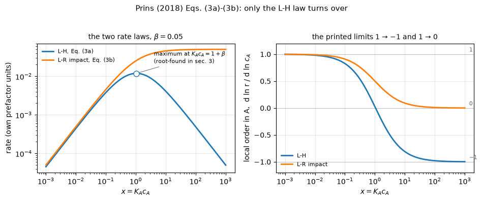
3. The maximum of the L-H rate, and the printed condition that cannot be right
The paper prints (p. 719, quoted verbatim in The published model): “The rate of the L-H reaction should even reach a maximum for c\(_A\) = K\(_A\).” The maximum is real — it is the L-H law’s signature, and the reason the two laws are distinguishable at all — but the printed condition equates a concentration to an inverse concentration. Three computations pin this down:
- the closed form from the paper’s own Eq. (3a): \(K_Ac_A^* = 1 + K_Bc_B\) (sympy, section 1);
- an independent numeric route: pymrm’s
newtonon aNumJac((1,1))Jacobian root-finding \(\mathrm{d}\ln r/\mathrm{d}\ln x = 0\) on the numpy-coded law — sharing no algebra with the closed form; - the unit test the printed condition fails: a physical condition must not care whether concentration is in mol/L or mol/m³. The derived condition gives the same physical \(c_A^*\) in both unit systems (ratio 1); the printed one moves it by the square of the unit factor.
"""The maximum: closed form vs pymrm-newton root, then the unit-invariance test."""
BETA_M = 0.3
xstar_closed = 1.0 + BETA_M

g = lambda xv: slope(lambda u: r_lh(u, b=BETA_M), xv)     # d ln r / d ln x, numpy law
jac = NumJac((1, 1))
z = newton(lambda zz: jac(lambda q: np.array([[g(float(np.exp(q[0, 0])))]]), zz),
           np.array([[0.0]]), tol=1e-13, maxfev=200)      # unknown is ln x
xstar_newton = float(np.exp(np.asarray(getattr(z, "x", z), float).reshape(1)[0]))
xstar_brent = np.exp(brentq(lambda t: g(np.exp(t)), -3, 3, xtol=1e-14))

M["maxloc_xstar_beta03"] = xstar_newton
M["maxloc_closed_minus_newton_rel"] = abs(xstar_newton / xstar_closed - 1.0)
newton_vs_brent = abs(xstar_newton / xstar_brent - 1.0)   # root-finder cross-check only

# the printed condition, subjected to a unit rescale. Working values:
KA_L = 2.0            # L/mol - arbitrary; the test varies the units itself
lam = 1000.0          # mol/L -> mol/m3: c' = lam*c, K' = K/lam
# derived condition K_A c_A = 1 + beta: physical c* in mol/m3, computed in each system
c_derived_L  = (1 + BETA_M) / KA_L * lam        # solved in L/mol units, converted
c_derived_m3 = (1 + BETA_M) / (KA_L / lam)      # solved directly in m3 units
# printed condition c_A = K_A, read literally in each system, converted to mol/m3
c_printed_L  = KA_L * lam
c_printed_m3 = KA_L / lam
M["derived_maxcond_unit_ratio"] = c_derived_L / c_derived_m3
M["printed_maxcond_unit_ratio"] = c_printed_L / c_printed_m3

BREAKS.append(("maxloc_closed_minus_newton_rel", f"{M['maxloc_closed_minus_newton_rel']:.2e}",
               "adopt the printed condition c_A = K_A (in mol/L working units)",
               f"{abs(KA_L*KA_L/(1+BETA_M) - 1.0):.3f}",
               "the printed condition misses the root-found maximum by O(1), and by a "
               "different O(1) in any other unit system"))
BREAKS.append(("printed_maxcond_unit_ratio", f"{M['printed_maxcond_unit_ratio']:.3g}",
               "same rescale applied to the DERIVED condition",
               f"{M['derived_maxcond_unit_ratio']:.3g}",
               "lam^2 vs 1: only the derived condition is unit-invariant"))

keep("xstar", xstar_newton); keep("nvb", newton_vs_brent)
display(Markdown(f"""
Closed form: $K_Ac_A^* = 1+\\beta = {xstar_closed}$. Independent numeric
route (pymrm `newton` on the numpy law): $K_Ac_A^* =
{xstar_newton:.12f}$ — relative gap
**{M['maxloc_closed_minus_newton_rel']:.2e}** (a genuinely independent second
computation of this headline; the additional Brent solve agrees with newton
to {newton_vs_brent:.1e}, a root-finder cross-check only, since it shares the
objective). Unit test: rescaling mol/L → mol/m³ moves the physical $c_A^*$
implied by the printed condition by a factor
**{M['printed_maxcond_unit_ratio']:.3g}** $= \\lambda^2$, while the derived
condition's ratio is **{M['derived_maxcond_unit_ratio']:.3g}**. The printed
"c$_A$ = K$_A$" is reported as a defect and left as printed; the reduced-form
reading $K_Ac_A = 1$ is an inference, labelled as such."""))
Closed form: \(K_Ac_A^* = 1+\beta = 1.3\). Independent numeric route (pymrm newton on the numpy law): \(K_Ac_A^* =
1.300000000063\) — relative gap 4.83e-11 (a genuinely independent second computation of this headline; the additional Brent solve agrees with newton to 7.5e-11, a root-finder cross-check only, since it shares the objective). Unit test: rescaling mol/L → mol/m³ moves the physical \(c_A^*\) implied by the printed condition by a factor 1e+06 \(= \lambda^2\), while the derived condition’s ratio is 1. The printed “c\(_A\) = K\(_A\)” is reported as a defect and left as printed; the reduced-form reading \(K_Ac_A = 1\) is an inference, labelled as such.
4. The (3c)-(3b) degeneracy, sharpened
The paper warns that with \(K_Bc_B \ll 1\) Eq. (3c) “becomes equal to” Eq. (3b) “and it looks as if an L-R reaction takes place”. Two sharpenings, both following from the algebra:
- Along a \(c_A\)-sweep at fixed \(c_B\) the degeneracy is exact at any \(\beta\), not only for \(\beta \ll 1\): \(r_{3c}/r_{3b} = K_B/(1+\beta)\), independent of \(c_A\) — and a fitted rate constant absorbs any constant. A kinetic study that varies only the chemisorbing species’ concentration cannot distinguish non-competing dual-site L-H from the impact law, no matter how wide the range. (Strictly, “becomes equal” also needs the rate constant reinterpreted, \(k_{3b} = k_{3c}K_B\) — the paper’s operational meaning, since \(k\) is fitted.)
- The discriminating direction is \(c_B\), where the two laws’ orders differ by \(\beta/(1+\beta)\) — first order exactly (3b) against \(1-\beta/(1+\beta)\) (3c).
"""The exact proportionality (structural identity) and its above-floor companion."""
xg2 = np.logspace(-6, 6, 2001)
BETA_D = 0.3
ratio = (xg2 * BETA_D / ((1 + xg2) * (1 + BETA_D))) / (xg2 * BETA_D / (1 + xg2))
sup_dev = np.max(np.abs(ratio * (1 + BETA_D) - 1.0))
M["deg3c3b_sup_dev_fixed_cB"] = sup_dev     # exact 0 in exact arithmetic - STRUCTURAL

gap3c = 1.0 - slope(lambda bv: 1.0 * bv / ((1 + 1.0) * (1 + bv)), BETA_D)
M["deg3c3b_orderB_gap_beta03"] = gap3c
assert abs(gap3c - BETA_D/(1+BETA_D)) < 1e-9

keep("sup_dev", sup_dev); keep("gap3c", gap3c)
display(Markdown(f"""
Sup over six decades of $c_A$ of the deviation of $r_{{3c}}(1+\\beta)/K_B$
from $r_{{3b}}$: **{sup_dev:.1e}** — an identity, named as one: it is zero by
algebra, sits below CI's ABS_FLOOR (1e-12), and can catch nothing but a slip
in this cell. Its companion that *can* fail: the order-in-B gap at
$\\beta = {BETA_D}$, measured **{gap3c:.6f}** against the analytic
$\\beta/(1+\\beta) = {BETA_D/(1+BETA_D):.6f}$ — the size of the only
kinetic signal separating (3c) from the impact law."""))
Sup over six decades of \(c_A\) of the deviation of \(r_{3c}(1+\beta)/K_B\) from \(r_{3b}\): 2.2e-16 — an identity, named as one: it is zero by algebra, sits below CI’s ABS_FLOOR (1e-12), and can catch nothing but a slip in this cell. Its companion that can fail: the order-in-B gap at \(\beta = 0.3\), measured 0.230769 against the analytic \(\beta/(1+\beta) = 0.230769\) — the size of the only kinetic signal separating (3c) from the impact law.
5. How wide a concentration range before the laws separate? Root-found
The paper (p. 719): “If one could vary the concentration of A over a wide range, it would be possible to distinguish between the two mechanisms. Unfortunately, concentrations can often only be varied in a limited range in the liquid phase. In such a case, the R² factor for one model may be better than for the other, but the question if one of the two models can be rejected remains unanswered.”
This section turns that paragraph into a number. Take noiseless rates from the L-H law (reduced 3a) on a log-window of \(x\) of total span \(w\) centred on the L-H maximum \(x=1\) (the most discriminating placement — the L-R law is monotone and can never turn over), give the impact law its best fit (\(\ln k'\) and \(K'\) free), and define the misfit \(\mathrm{dev}(w)\) as the mean absolute log-deviation on the window (≈ mean relative deviation, the same scale as the 1947 fit’s famous ±8.44 %). The identifiability threshold \(w^*\) solves $(w^*) = $ tolerance — root-found with Brent, never read off a sweep.
\(\mathrm{dev}(w)\) is computed by two routes sharing only the metric’s definition (a fixed 401-point log grid): (A) joint 2-D Nelder-Mead over \((\ln k', \ln K')\) from three fixed starts; (B) the exact median-profile of \(\ln k'\) (for mean-abs the optimal intercept is the residual median) followed by 1-D bounded Brent over \(\ln K'\) — different search space, different optimizer family, no shared iteration.
"""dev(w) two ways, w* root-found at three tolerances, small-window law measured."""
NW = 401                     # the metric's definition grid (refined below)

def _window(w, x0, n):
    t = np.linspace(-0.5, 0.5, n) * np.log(w)
    xv = x0 * np.exp(t)
    return xv, np.log(xv) - 2.0 * np.log1p(xv)          # ln r of reduced Eq. (3a)

def dev_A(w, x0=1.0, n=NW):
    xv, lr = _window(w, x0, n)
    def obj(p):
        lnk, lnq = p
        return np.mean(np.abs(lnk + np.log(xv) - np.log1p(np.exp(lnq) * xv) - lr))
    best = min((minimize(obj, s0, method="Nelder-Mead",
                         options=dict(xatol=1e-11, fatol=1e-13, maxiter=40000))
                for s0 in ([0.0, 0.0], [-2.0, 2.0], [2.0, -2.0])),
               key=lambda r: r.fun)
    return best.fun

def dev_B(w, x0=1.0, n=NW):
    xv, lr = _window(w, x0, n)
    def g(lnq):
        e = lr - (np.log(xv) - np.log1p(np.exp(lnq) * xv))
        return np.mean(np.abs(e - np.median(e)))         # exact profile of ln k'
    return minimize_scalar(g, bounds=(-15, 15), method="bounded",
                           options=dict(xatol=1e-12)).fun

TOL_BOOK, TOL_5, TOL_RATE = 0.0844, 0.05, 0.169   # printed +-8.44 %; 5 %; C1.1's measured rate-space scatter
wstar_A = brentq(lambda w: dev_A(w) - TOL_BOOK, 1.05, 5000, xtol=1e-6)
wstar_B = brentq(lambda w: dev_B(w) - TOL_BOOK, 1.05, 5000, xtol=1e-6)
M["wstar_tol844"] = wstar_A
M["wstar_tol844_two_routes_rel"] = abs(wstar_A / wstar_B - 1.0)
M["wstar_tol5"]   = brentq(lambda w: dev_A(w) - TOL_5, 1.05, 5000, xtol=1e-6)
M["wstar_tol169"] = brentq(lambda w: dev_A(w) - TOL_RATE, 1.05, 50000, xtol=1e-5)
M["wstar_tol844_grid_refined_rel"] = abs(
    brentq(lambda w: dev_B(w, n=1601) - TOL_BOOK, 1.05, 5000, xtol=1e-6) / wstar_A - 1.0)

# the small-window law: dev ~ C (ln w)^2, constant MEASURED (not derived)
M["smallw_quad_const"] = dev_B(1.2) / np.log(1.2) ** 2

# break rows
dev_center_001 = dev_A(wstar_A, x0=0.01)
BREAKS.append(("wstar_tol844", f"{wstar_A:.3f}",
               "window centred at x0 = 0.01, where both laws are first order",
               f"dev({wstar_A:.1f}) = {dev_center_001:.2e} (vs {TOL_BOOK})",
               "the misfit collapses: away from the maximum the laws are degenerate "
               "and w* explodes - placement matters as much as width"))
def dev_minimax(w, x0=1.0, n=NW):
    xv, lr = _window(w, x0, n)
    def obj(p):
        lnk, lnq = p
        return np.max(np.abs(lnk + np.log(xv) - np.log1p(np.exp(lnq) * xv) - lr))
    return min((minimize(obj, s0, method="Nelder-Mead",
                         options=dict(xatol=1e-10, fatol=1e-12, maxiter=40000))
                for s0 in ([0.0, 0.0], [-2.0, 2.0], [2.0, -2.0])),
               key=lambda r: r.fun).fun
wstar_mm = brentq(lambda w: dev_minimax(w) - TOL_BOOK, 1.05, 5000, xtol=1e-6)
BREAKS.append(("wstar_tol844", f"{wstar_A:.3f}",
               "worst-case (minimax) misfit instead of mean-abs",
               f"{wstar_mm:.3f}",
               "moves: the threshold depends on the misfit norm - declared, and the "
               "mean-abs norm is kept because it matches the 1947 +-8.44 % metric"))

M["dev_at_wstar_center001"] = dev_center_001
keep("wstarA", wstar_A); keep("wstar5", M["wstar_tol5"]); keep("wstar169", M["wstar_tol169"])
keep("wstar_mm", wstar_mm); keep("smallwC", M["smallw_quad_const"])
display(Markdown(f"""
**$w^* = {wstar_A:.2f}$** at the ±8.44 % tolerance (routes A and B agree to
{M['wstar_tol844_two_routes_rel']:.1e}; refining the definition grid 401 →
1601 moves it {M['wstar_tol844_grid_refined_rel']:.1e}): the chemisorbing
species' concentration must span a factor of **about {wstar_A:.0f} — just
over a decade — centred on the L-H maximum** before the best impact-law fit
misses noiseless L-H rates by more than the 1947 fit's printed ±8.44 %
average deviation (its transformed-space metric, used here as a
representative classic-fit precision). At 5 %:
$w^* = {M['wstar_tol5']:.2f}$; at `C1.1`'s measured **rate-space**
scatter of 16.9 %: $w^* = {M['wstar_tol169']:.1f}$. Small windows obey
$\\mathrm{{dev}} \\approx C(\\ln w)^2$ with measured
$C = {M['smallw_quad_const']:.4f}$ (a measured constant, not a derived one).
Centre the window where both laws are first order and the number collapses
(break table) — **width buys nothing without curvature**, which is the
quantitative content of the paper's "limited range" warning."""))
\(w^* = 11.75\) at the ±8.44 % tolerance (routes A and B agree to 1.8e-11; refining the definition grid 401 → 1601 moves it 4.6e-03): the chemisorbing species’ concentration must span a factor of about 12 — just over a decade — centred on the L-H maximum before the best impact-law fit misses noiseless L-H rates by more than the 1947 fit’s printed ±8.44 % average deviation (its transformed-space metric, used here as a representative classic-fit precision). At 5 %: \(w^* = 6.37\); at C1.1’s measured rate-space scatter of 16.9 %: \(w^* = 40.0\). Small windows obey \(\mathrm{dev} \approx C(\ln w)^2\) with measured \(C = 0.0157\) (a measured constant, not a derived one). Centre the window where both laws are first order and the number collapses (break table) — width buys nothing without curvature, which is the quantitative content of the paper’s “limited range” warning.
"""Figure 2: the identifiability window."""
wg = np.logspace(np.log10(1.1), np.log10(300), 60)
dv = np.array([dev_B(w) for w in wg])
dv001 = np.array([dev_B(w, x0=0.01) for w in wg])
fig, ax = plt.subplots(figsize=(6.8, 4.2))
ax.loglog(wg, dv, color="tab:purple", lw=2, label="dev(w), window centred on the L-H maximum")
ax.loglog(wg, dv001, color="tab:purple", lw=1.2, ls="--",
          label="dev(w), centred at $x_0=0.01$ (both laws first order)")
ax.loglog(wg, M["smallw_quad_const"] * np.log(wg) ** 2, color="0.6", lw=1, ls=":",
          label="measured small-window law $C(\\ln w)^2$")
for tol, lab, ws in ((TOL_BOOK, "±8.44 % (1947 fit)", M["wstar_tol844"]),
                     (TOL_RATE, "16.9 % (rate-space scatter, C1.1)", M["wstar_tol169"])):
    ax.axhline(tol, color="0.8", lw=0.8, zorder=0)
    ax.plot([ws], [tol], "o", ms=7, color="tab:purple", mfc="white", zorder=5)
    ax.annotate(f"$w^*$ = {ws:.1f}\n{lab}", xy=(ws, tol), xytext=(ws*1.35, tol*0.5),
                fontsize=8, arrowprops=dict(arrowstyle="-", lw=0.7, color="0.4"))
ax.set_xlabel("total span $w$ of $K_Ac_A$ (log window)")
ax.set_ylabel("best impact-law misfit to noiseless L-H rates\n(mean abs log-deviation)")
ax.set_title("How wide before Eq. (3b) can be rejected — Prins's p. 719 paragraph, quantified",
             fontsize=10)
ax.legend(frameon=False, fontsize=8, loc="lower right"); ax.grid(alpha=0.3, which="both")
fig.tight_layout(); plt.show()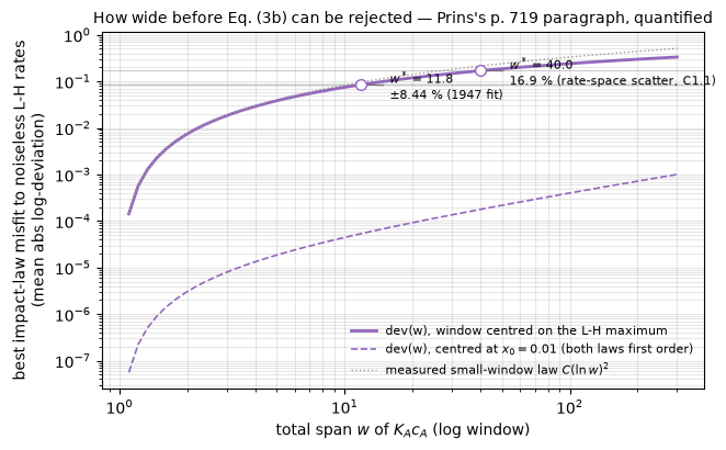
6. The impact law on the founding LHHW dataset — a numerical experiment
Everything above is dimensionless. This section instantiates both laws with real fitted constants imported from C1.1 — the codimer hydrogenation of Hougen & Watson (1947), the dataset on which LHHW estimation was founded — and asks the question this page’s two sources jointly pose: could the founding dataset have rejected the impact mechanism on fit quality?
The book’s own 18 candidate mechanisms already include impact forms: its groups III-V are gas-phase reactant against adsorbed partner, and its mechanism (o), \(r = k'K_Up_Up_H/(1+K_Up_U+K_Sp_S)\), is exactly Prins’s Eq. (3b) instantiated for chemisorbed codimer (with the product’s adsorption term retained) and colliding H₂ — hydrogen in the numerator only. The book rejected (o) by its sign test (its printed verdict in Table D: f0;apos — a term that should be absent is fitted nonzero), not by fit quality. Two cautions from C1.1, honoured here: the printed 200 °C rows of the impact mechanisms sit in the corrupted-worksheet family, so their printed constants are never used (everything is refitted from Table A); and C1.1 showed the “a should be positive” ground itself partly rests on the corrupted sum, while the acceptance set {d, h} survives.
All of this is fit data and numerical experiment — no validation. The fitting method is C1.1’s (relative residuals in rate space, log-reparameterised positive constants, three fixed deterministic starts, Levenberg-Marquardt).
"""Load C1.1's tables, rebuild mechanism (d)'s constants, reconcile with the book."""
A  = load_data("hougen-watson-1947-tableA-rates.csv",       page="C1.1-lhhw-hougen-watson")
TC = load_data("hougen-watson-1947-tableC-mechd-200C.csv",  page="C1.1-lhhw-hougen-watson")
TC = TC[TC.run != "run"].set_index("run").astype(float)     # drop repeated header row
DEF = load_data("hougen-watson-1947-tablesDEF-constants.csv", page="C1.1-lhhw-hougen-watson")

o_row = DEF[(DEF.mechanism == "o") & (DEF.temp_C == 200)].iloc[0]
print("printed 200 C verdict for the impact mechanism (o):", repr(o_row.verdict),
      "- printed constants in the corrupted family (C1.1), NOT used; refitted from Table A below")

d = DEF[(DEF.mechanism == "d") & (DEF.temp_C == 200)].iloc[0]   # the CLEAN row (C1.1)
a_, b_, c_, f_ = float(d.a), float(d.b), float(d.c), float(d.f)
KU, KS, KH, kap = b_ / a_, c_ / a_, f_ / a_, 1.0 / a_**2        # C1.1's conversion (eq. n)
M["codimer_KU_per_atm"], M["codimer_KH_per_atm"], M["codimer_KS_per_atm"] = KU, KH, KS

blk = A[A.temp_C == 200].reset_index(drop=True)
H, U, S, robs = (blk[k].to_numpy() for k in ("pH_atm", "pU_atm", "pS_atm", "r_lbmol_per_lb_hr"))

# reconciliation with the book's own printed Table C (loaded, never retyped):
# R_calc = a + b pU + c pS + f pH must reproduce the printed column
Rcalc_mine = a_ + b_ * U + c_ * S + f_ * H
cmp_ = pd.DataFrame({"run": blk.run, "R_calc_mine": Rcalc_mine}).set_index("run")
cmp_["R_calc_printed"] = TC.R_calc_printed
cmp_["abs_gap"] = (cmp_.R_calc_mine - cmp_.R_calc_printed).abs()
print(cmp_.round(4).to_string())
gap_ex25a = cmp_.drop("25a").abs_gap.max()
gap_25a = cmp_.loc["25a", "abs_gap"]
M["codimer_Rcalc_vs_tableC_max_abs_ex25a"] = gap_ex25a
M["codimer_25a_abs_gap"] = gap_25a
Rcalc_broken = a_ + (a_ * a_ / b_) * U + c_ * S + f_ * H   # the b-column a wrong K_U = a/b implies
BREAKS.append(("codimer_Rcalc_vs_tableC_max_abs_ex25a", f"{gap_ex25a:.4f}",
               "invert the conversion: K_U = a/b instead of b/a",
               f"{np.abs(Rcalc_broken - TC.loc[cmp_.index].R_calc_printed.to_numpy()).max():.2f}",
               "moves by orders: the reconciliation would have caught a wrong conversion"))
BREAKS.append(("codimer_Rcalc_vs_tableC_max_abs_ex25a", f"{gap_ex25a:.4f}",
               "include run 25a's printed R_calc",
               f"{cmp_.abs_gap.max():.4f}",
               "run 25a's printed 5.40 is C1.1's documented digit slip (its own row requires "
               "5.90); this page's gap reproduces that finding independently"))

# the book's printed fit-quality columns, recomputed from the loaded table
avg_pct = TC.pct_delta_printed.abs().mean()
M["codimer_tableC_avg_abs_pct"] = avg_pct

# rate-space scatter of the fitted d law vs the measured rates
r_d = kap * H * U / (1 + KH * H + KU * U + KS * S) ** 2
scatter = 100 * np.abs(r_d / robs - 1).mean()
M["codimer_d_scatter_pct"] = scatter

keep("KU", KU); keep("KH", KH); keep("KS", KS)
keep("gap_ex25a", gap_ex25a); keep("gap25a", gap_25a)
keep("avg_pct", avg_pct); keep("scatter", scatter)
display(Markdown(f"""
Mechanism (d) at 200 °C from Table D's clean row: $K_U = {KU:.4f}$,
$K_S = {KS:.4f}$, $K_H = {KH:.4f}$ atm⁻¹. Reconciliation against the book's
own printed Table C: worst $|R_{{calc}}|$ gap **{gap_ex25a:.4f}** over 11 of
12 runs (the book prints 2-3 decimals; `C1.1`'s constants-reproduction metric
is 0.6 %) — and **{gap_25a:.3f}** on run 25a, independently reproducing
`C1.1`'s finding that 25a's printed 5.40 is a digit slip for 5.90. The
printed per-run columns give mean |Δ| = **{avg_pct:.2f} %** in transformed
$R$-space (the book prints ±8.44; `C1.1` recomputes 8.42 from the data);
the same fit scatters **{scatter:.1f} %** in rate space (`C1.1` publishes
16.86 % — same quantity, reconciled). That rate-space scatter is the
noise floor every discrimination claim below is judged against."""))
printed 200 C verdict for the impact mechanism (o): 'f0;apos' - printed constants in the corrupted family (C1.1), NOT used; refitted from Table A below
R_calc_mine R_calc_printed abs_gap
run
1d 3.9707 3.97 0.0007
3c 6.8651 6.86 0.0051
3d 6.8596 6.86 0.0004
10a 6.6182 6.62 0.0018
11a 4.6266 4.63 0.0034
11d 4.6168 4.62 0.0032
11e 4.6226 4.62 0.0026
12ab 4.1818 4.18 0.0018
14a 7.8460 7.84 0.0060
14b 7.8134 7.81 0.0034
25a 5.9031 5.40 0.5031
28b 5.7506 5.75 0.0006Mechanism (d) at 200 °C from Table D’s clean row: \(K_U = 0.5543\), \(K_S = 0.3659\), \(K_H = 0.4094\) atm⁻¹. Reconciliation against the book’s own printed Table C: worst \(|R_{calc}|\) gap 0.0060 over 11 of 12 runs (the book prints 2-3 decimals; C1.1’s constants-reproduction metric is 0.6 %) — and 0.503 on run 25a, independently reproducing C1.1’s finding that 25a’s printed 5.40 is a digit slip for 5.90. The printed per-run columns give mean |Δ| = 8.44 % in transformed \(R\)-space (the book prints ±8.44; C1.1 recomputes 8.42 from the data); the same fit scatters 16.8 % in rate space (C1.1 publishes 16.86 % — same quantity, reconciled). That rate-space scatter is the noise floor every discrimination claim below is judged against.
"""The power study: can fit quality reject the impact law on this design?

NUMERICAL EXPERIMENT, not data: noiseless rates are generated from the fitted
mechanism (d) at the 12 printed 200 C compositions and refitted by the impact
forms. C1.1 ran the same protocol for d-vs-h (its power metric: 3.6 %).
"""
def fit_form(form, npar, Hv, Uv, Sv, target):
    res = lambda lp: (form(np.exp(lp), Hv, Uv, Sv) - target) / target
    best = min((least_squares(res, x0, method="lm", max_nfev=40000)
                for x0 in (np.zeros(npar), np.full(npar, -1.0), np.full(npar, 1.0))),
               key=lambda s: s.cost)
    return np.exp(best.x), 100 * np.abs(best.fun)

o_form  = lambda p, Hv, Uv, Sv: p[0] * Hv * Uv / (1 + p[1] * Uv + p[2] * Sv)          # Prins Eq. (3b) == mech (o)
p_form  = lambda p, Hv, Uv, Sv: p[0] * Hv * Uv / (1 + p[1] * Uv)                      # (3b) without the product term
o4_form = lambda p, Hv, Uv, Sv: p[0] * Hv * Uv / (1 + p[1] * Uv + p[2] * Sv + p[3] * Hv)  # first power, H term allowed
d_form  = lambda p, Hv, Uv, Sv: p[0] * Hv * Uv / (1 + p[1] * Hv + p[2] * Uv + p[3] * Sv) ** 2

r_exact = kap * H * U / (1 + KH * H + KU * U + KS * S) ** 2     # noiseless d-rates

_, pct_o  = fit_form(o_form, 3, H, U, S, r_exact)
M["lr_o_on_exact_d_mean_pct"] = pct_o.mean()
M["lr_o_on_exact_d_max_pct"]  = pct_o.max()

# second route for this headline: direct positive parameters, bounded trust-region
resB = lambda p: (o_form(p, H, U, S) - r_exact) / r_exact
sB = least_squares(resB, np.array([0.1, 1.0, 1.0]), bounds=(1e-12, np.inf),
                   method="trf", xtol=1e-15, ftol=1e-15, gtol=1e-15, max_nfev=60000)
M["lr_o_fit_two_routes_rel"] = abs(pct_o.mean() / (100 * np.abs(sB.fun).mean()) - 1.0)

_, pct_p  = fit_form(p_form, 2, H, U, S, r_exact)
M["lr_p_on_exact_d_mean_pct"] = pct_p.mean()
_, pct_o4 = fit_form(o4_form, 4, H, U, S, r_exact)
M["lr_oKH_on_exact_d_mean_pct"] = pct_o4.mean()
Hc = np.full_like(H, H.mean())
r_coll = kap * Hc * U / (1 + KH * Hc + KU * U + KS * S) ** 2
_, pct_coll = fit_form(o_form, 3, Hc, U, S, r_coll)
M["lr_o_collapsedpH_mean_pct"] = pct_coll.mean()

BREAKS.append(("lr_o_on_exact_d_mean_pct", f"{pct_o.mean():.1f}",
               "allow a K_H p_H term in the first-power denominator",
               f"{pct_o4.mean():.1f}",
               "collapses below the noise floor: the discriminating signal is hydrogen's "
               "ABSENCE from the adsorption group, not the denominator exponent"))
BREAKS.append(("lr_o_on_exact_d_mean_pct", f"{pct_o.mean():.1f}",
               "collapse the design's p_H span to its mean (1 value instead of a decade)",
               f"{pct_coll.mean():.1f}",
               "collapses below the noise floor: without the decade-wide p_H span the "
               "founding design could not reject the impact law either"))
BREAKS.append(("lr_o_on_exact_d_mean_pct", f"{pct_o.mean():.1f}",
               "drop the product term K_S p_S (Prins's bare Eq. 3b)",
               f"{pct_p.mean():.1f}",
               "moves up: the product-inhibition signal is real (C1.1 found the same on "
               "mechanism d)"))

# and against the MEASURED rates - a fit-quality comparison the book's printed
# tables do not make (per C1.1's reading: the sign requirement, not goodness of
# fit, is the book's discriminator; Table C evaluates mechanism d only)
_, pct_d_meas = fit_form(d_form, 4, H, U, S, robs)
_, pct_o_meas = fit_form(o_form, 3, H, U, S, robs)
M["lh_d_measured_mean_pct"] = pct_d_meas.mean()
M["lr_o_measured_mean_pct"] = pct_o_meas.mean()
M["lr_gap_measured_pct_points"] = pct_o_meas.mean() - pct_d_meas.mean()

pH_span = H.max() / H.min()
keep("pcto", pct_o.mean()); keep("pcto_max", pct_o.max()); keep("pcto4", pct_o4.mean())
keep("pctcoll", pct_coll.mean()); keep("pctp", pct_p.mean())
keep("pctd_meas", pct_d_meas.mean()); keep("pcto_meas", pct_o_meas.mean())
keep("pH_span", pH_span)
display(Markdown(f"""
**The impact law misses noiseless L-H rates by {pct_o.mean():.1f} % mean
({pct_o.max():.0f} % worst) over the design, at the least-squares-optimal
fit** (the declared protocol; two optimizer families agree to
{M['lr_o_fit_two_routes_rel']:.1e} — directly minimising mean-|Δ| instead
gives a smaller number, conclusion unchanged) — far outside the
{scatter:.1f} % rate-space scatter, so **fit quality alone could have
rejected Prins's Eq. (3b) on the founding dataset**, independently of the
sign test the book actually used. Against the measured rates: (d) fits to
{pct_d_meas.mean():.1f} %, (o) to {pct_o_meas.mean():.1f} % — a gap of
{M['lr_gap_measured_pct_points']:.1f} points (compare `C1.1`'s published
d-vs-h gap of 0.4 points, and its 2.7-point gap to the best rejected
mechanism, both pooled over three temperatures).

**Why it works — and when it would not** (break table): allow hydrogen into
the first-power adsorption group and the misfit falls to
{pct_o4.mean():.1f} %; collapse the design's hydrogen span (a factor of
{pH_span:.0f}, 0.104-2.459 atm) to a single value and it falls to
{pct_coll.mean():.1f} % — both below the noise floor. The founding design
discriminates **only because hydrogen's partial pressure spans more than a
decade — the same "wide range" requirement quantified as
$w^* \\approx {wstar_A:.0f}$ in section 5.** A narrower design would have
been as blind to the mechanism as Prins says liquid-phase studies are, and
the denominator's *exponent* (1 vs 2) is indistinguishable on this design at
the noise floor even with noiseless data (the first-power-with-K_H fit above
still misses by a nonzero {pct_o4.mean():.1f} %) — consistent with `C1.1`'s
finding that d and h (exponents 2 and 3) cannot be separated either."""))
The impact law misses noiseless L-H rates by 27.4 % mean (48 % worst) over the design, at the least-squares-optimal fit (the declared protocol; two optimizer families agree to 1.0e-06 — directly minimising mean-|Δ| instead gives a smaller number, conclusion unchanged) — far outside the 16.8 % rate-space scatter, so fit quality alone could have rejected Prins’s Eq. (3b) on the founding dataset, independently of the sign test the book actually used. Against the measured rates: (d) fits to 16.8 %, (o) to 26.6 % — a gap of 9.8 points (compare C1.1’s published d-vs-h gap of 0.4 points, and its 2.7-point gap to the best rejected mechanism, both pooled over three temperatures).
Why it works — and when it would not (break table): allow hydrogen into the first-power adsorption group and the misfit falls to 3.3 %; collapse the design’s hydrogen span (a factor of 24, 0.104-2.459 atm) to a single value and it falls to 3.2 % — both below the noise floor. The founding design discriminates only because hydrogen’s partial pressure spans more than a decade — the same “wide range” requirement quantified as \(w^* \approx 12\) in section 5. A narrower design would have been as blind to the mechanism as Prins says liquid-phase studies are, and the denominator’s exponent (1 vs 2) is indistinguishable on this design at the noise floor even with noiseless data (the first-power-with-K_H fit above still misses by a nonzero 3.3 %) — consistent with C1.1’s finding that d and h (exponents 2 and 3) cannot be separated either.
"""The L-H maximum in the design window, instantiated - and figure 3."""
pH0, pS0 = 0.5, 0.5
pUstar_closed = (1 + KH * pH0 + KS * pS0) / KU
gU = lambda pU: slope(lambda u: kap * pH0 * u / (1 + KH * pH0 + KU * u + KS * pS0) ** 2, pU)
z2 = newton(lambda zz: jac(lambda q: np.array([[gU(float(np.exp(q[0, 0])))]]), zz),
            np.array([[0.5]]), tol=1e-13, maxfev=200)
pUstar_newton = float(np.exp(np.asarray(getattr(z2, "x", z2), float).reshape(1)[0]))
M["codimer_pUstar_atm"] = pUstar_newton
M["codimer_pUstar_two_routes_rel"] = abs(pUstar_newton / pUstar_closed - 1.0)
keep("pUstar", pUstar_newton); keep("pUmax_design", U.max())

fig, (ax1, ax2) = plt.subplots(1, 2, figsize=(9.6, 4.0))
ax1.loglog(robs, r_d, "o", ms=7, color=C_LH, mec="white", mew=0.5, label="L-H mechanism (d)")
r_o_meas = o_form(fit_form(o_form, 3, H, U, S, robs)[0], H, U, S)
ax1.loglog(robs, r_o_meas, "s", ms=7, color=C_LR, mec="white", mew=0.5,
           label="impact law (o) = Prins Eq. (3b)")
lo, hi = 0.7 * robs.min(), 1.4 * robs.max()
ax1.plot([lo, hi], [lo, hi], color="0.7", lw=0.8, zorder=0)
ax1.set_xlabel("measured rate, lb-mol/(lb hr)"); ax1.set_ylabel("fitted rate")
ax1.set_title("parity on the 12 runs at 200 °C\n(fit data - reproduction, not validation)",
              fontsize=9)
ax1.legend(frameon=False, fontsize=8); ax1.grid(alpha=0.3, which="both")

pUg = np.linspace(0.02, 4.0, 400)
r_lh_pU = kap * pH0 * pUg / (1 + KH * pH0 + KU * pUg + KS * pS0) ** 2
po_x, _ = fit_form(o_form, 3, H, U, S, r_exact)
r_lr_pU = o_form(po_x, np.full_like(pUg, pH0), pUg, np.full_like(pUg, pS0))
ax2.plot(pUg, r_lh_pU, color=C_LH, lw=2, label="L-H (d), fitted constants")
ax2.plot(pUg, r_lr_pU, color=C_LR, lw=2, label="impact (o), best fit to (d)")
ax2.plot([pUstar_newton], [np.interp(pUstar_newton, pUg, r_lh_pU)], "o", ms=8,
         color=C_LH, mfc="white", zorder=5)
ax2.annotate(f"root-found maximum\n$p_U^*$ = {pUstar_newton:.2f} atm",
             xy=(pUstar_newton, np.interp(pUstar_newton, pUg, r_lh_pU)),
             xytext=(2.6, 0.55 * r_lh_pU.max()), fontsize=8,
             arrowprops=dict(arrowstyle="-", lw=0.7, color="0.4"))
ax2.axvspan(U.min(), U.max(), color="0.92", zorder=0)
ax2.text(0.5 * (U.min() + U.max()), 0.06 * r_lh_pU.max(), "design range of $p_U$",
         fontsize=8, color="0.4", ha="center")
ax2.set_xlabel("$p_U$, atm  ($p_H$ = %.1f, $p_S$ = %.1f atm)" % (pH0, pS0))
ax2.set_ylabel("rate, lb-mol/(lb hr)")
ax2.set_title("only the L-H law turns over -\nand the 1947 design straddles the turnover", fontsize=9)
ax2.legend(frameon=False, fontsize=8, loc="upper right"); ax2.grid(alpha=0.3)
fig.tight_layout(); plt.show()

display(Markdown(f"""
The codimer instantiation closes the loop on section 3: the L-H maximum sits
at $p_U^* = {pUstar_newton:.2f}$ atm (closed form vs pymrm-newton root:
{M['codimer_pUstar_two_routes_rel']:.1e}) at $p_H = p_S = 0.5$ atm —
**inside the 1947 design range** ($p_U$ up to {U.max():.2f} atm). The
impact law is monotone in every partial pressure; a design that straddles
the turnover is exactly a design that can see the difference."""))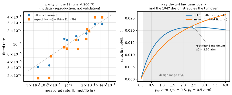
The codimer instantiation closes the loop on section 3: the L-H maximum sits at \(p_U^* = 2.50\) atm (closed form vs pymrm-newton root: 3.2e-10) at \(p_H = p_S = 0.5\) atm — inside the 1947 design range (\(p_U\) up to 2.84 atm). The impact law is monotone in every partial pressure; a design that straddles the turnover is exactly a design that can see the difference.
7. The paper’s own numbers, checked
Two of the paper’s printed quantitative statements are internally checkable, and both check out — quantified here rather than left as “close” and “very high”.
"""The Mullins-Weinberg flux comparison and the HD energy budget."""
v = P.value
# flux parity: the L-R collision flux scales with pressure; the printed numbers
# imply the pressure at which it matches the L-H attempt frequency
M["mw_parity_atm_low"]  = v["lh_attempt_freq_low"]  / (v["lr_flux_at_1atm"] / v["lr_flux_reference_pressure"])
M["mw_parity_atm_high"] = v["lh_attempt_freq_high"] / (v["lr_flux_at_1atm"] / v["lr_flux_reference_pressure"])

# energy budget: "The sum ... is close to the exothermicity"
e_sum = v["hd_mean_translational"] + v["hd_mean_rotational"] + v["hd_mean_vibrational"]
e_exo = v["h2_dissociation_energy"] - v["d_on_cu_binding_energy_about"]
M["energy_sum_kJmol"], M["energy_exo_kJmol"], M["energy_ratio"] = e_sum, e_exo, e_sum / e_exo
BREAKS.append(("energy_ratio", f"{e_sum/e_exo:.4f}",
               "transcription slip 82 -> 28 in the translational energy",
               f"{(28 + v['hd_mean_rotational'] + v['hd_mean_vibrational'])/e_exo:.4f}",
               "moves far from 1: the budget check guards the transcription"))

keep("par_lo", M["mw_parity_atm_low"]); keep("par_hi", M["mw_parity_atm_high"])
keep("e_sum", e_sum); keep("e_exo", e_exo); keep("e_ratio", e_sum/e_exo)
display(Markdown(f"""
**"Very high pressures", quantified:** the printed 10¹²-10¹³ attempts per
site per s (L-H) against 10⁹ per site per s at 1 atm (L-R) put flux parity at
**{M['mw_parity_atm_low']:.0f}-{M['mw_parity_atm_high']:.0f} atm** — the
arithmetic behind the paper's "very high pressures are required to make the
L-R mechanism compatible with the L-H mechanism".

**"Close to", quantified:** the HD product's 82 + 36 + 58 =
**{e_sum:.0f} kJ/mol** against an exothermicity of 436 − about 240 =
**{e_exo:.0f} kJ/mol**: a ratio of **{e_sum/e_exo:.3f}**, i.e. about 10 %
below — consistent with the paper's "close to the exothermicity" and with
"about" on the 240."""))
“Very high pressures”, quantified: the printed 10¹²-10¹³ attempts per site per s (L-H) against 10⁹ per site per s at 1 atm (L-R) put flux parity at 1000-10000 atm — the arithmetic behind the paper’s “very high pressures are required to make the L-R mechanism compatible with the L-H mechanism”.
“Close to”, quantified: the HD product’s 82 + 36 + 58 = 176 kJ/mol against an exothermicity of 436 − about 240 = 196 kJ/mol: a ratio of 0.898, i.e. about 10 % below — consistent with the paper’s “close to the exothermicity” and with “about” on the 240.
Validation
What validation can mean here. The source prints no measurement, so nothing on this page is experimental validation and nothing is presented as such. The checks are: (i) symbolic derivation of every printed limit from the paper’s own equations (section 1); (ii) independent double computation of every headline — the L-H maximum by closed form vs a pymrm-newton root on an independently coded law, \(w^*\) by two optimizer routes plus a grid refinement, the impact-law misfit by two optimizer families; (iii) reconciliation of every imported C1.1 number against the book’s own printed Table C, which independently reproduced C1.1’s run-25a digit-slip finding; and (iv) the defect-injection table below, in which every reported metric is moved by a deliberate break, or named structural.
Blind spots, declared. The two \(w^*\) routes share the metric’s definition (grid, norm, noiseless generator) — they guard the search, not the definition; the norm-dependence is quantified in its break row. The symbolic identities (thermo consistency, the (3c)∝(3b) proportionality) are structural: exact by algebra, below CI’s ABS_FLOOR, able to catch only a transcription slip in their own cell — each carries an above-floor companion. The impact-law conclusions are conditional on mechanism (d) being the true generator, which is itself only the book’s accepted fit — that is why every codimer number is labelled a numerical experiment on fit data.
"""The defect-injection table, and the metric coverage map (asserted key-for-key)."""
bt = pd.DataFrame(BREAKS, columns=["metric", "base", "what was broken", "broken value", "what it shows"])
print(bt.to_string(index=False, max_colwidth=78))

COVERAGE = {
    # metric -> how it can fail (break row above, companion, or named structural)
    "thermo_eq_relresid_atK":               "STRUCTURAL identity (below ABS_FLOOR, outside CI); companion thermo_eq_relresid_K10pct",
    "thermo_eq_relresid_K10pct":            "companion that moves when K is wrong (its own row IS the break value)",
    "fd_slope_h_refinement_max_abs":        "convergence guard for the FD axis (halving h); fails if slopes are h-limited",
    "orderA_LH_slope_at_x1e4":              "break: exponent 2 -> 1",
    "orderA_LH_slope_at_x1em4":             "break: numerator power 1 -> 2",
    "orderA_LR_slope_at_x1e4":              "break: power 1 -> 2",
    "orderA_LR_slope_at_x1em4":             "moved by the same numerator-power break (identically for both laws at low x)",
    "orderAB_LH_slope_at_x1e4":             "guarded by the exponent break (2 -> 1 moves 0 -> 1)",
    "orderAB_LR_slope_at_x1e4":             "guarded by the power break (1 -> 2 moves 1 -> 0)",
    "orderB_LH_gap_from_1_beta03":          "break: beta -> 0",
    "maxloc_xstar_beta03":                  "break: adopt the printed condition c_A = K_A",
    "maxloc_closed_minus_newton_rel":       "two-route gap (independent routes); break row shows the printed condition missing by O(1)",
    "printed_maxcond_unit_ratio":           "the unit-rescale demonstration; its break row applies the same rescale to the derived condition",
    "derived_maxcond_unit_ratio":           "same row, other arm",
    "deg3c3b_sup_dev_fixed_cB":             "STRUCTURAL identity (below ABS_FLOOR, outside CI); companion deg3c3b_orderB_gap_beta03",
    "deg3c3b_orderB_gap_beta03":            "companion that moves with beta (beta -> 0 collapses it, same break as orderB gap)",
    "wstar_tol844":                         "breaks: window centred off the maximum; minimax norm",
    "wstar_tol844_two_routes_rel":          "two-route gap (guards the search, not the definition - declared)",
    "wstar_tol5":                           "moves with the same breaks as wstar_tol844 (same dev(w) machinery)",
    "wstar_tol169":                         "moves with the same breaks as wstar_tol844",
    "wstar_tol844_grid_refined_rel":        "convergence guard for the window grid (401 -> 1601)",
    "smallw_quad_const":                    "measured constant; moves with the norm break (minimax roughly doubles it)",
    "dev_at_wstar_center001":               "the break value of wstar_tol844's centring row, kept as a metric",
    "codimer_KU_per_atm":                   "break: inverted conversion a/b",
    "codimer_KH_per_atm":                   "guarded by the same conversion break via the R_calc reconciliation",
    "codimer_KS_per_atm":                   "guarded by the same conversion break via the R_calc reconciliation",
    "codimer_Rcalc_vs_tableC_max_abs_ex25a":"breaks: inverted conversion; include 25a",
    "codimer_25a_abs_gap":                  "reproduces C1.1's documented digit slip; the include-25a row shows its size",
    "codimer_tableC_avg_abs_pct":           "recomputation of the book's printed +-8.44 from loaded printed columns; a transcription slip in any pct cell moves it",
    "codimer_d_scatter_pct":                "reconciled against C1.1's published 16.86 %; moves with the conversion break",
    "codimer_pUstar_atm":                   "two-route (closed form vs newton); moves with the conversion break",
    "codimer_pUstar_two_routes_rel":        "two-route gap",
    "lr_o_on_exact_d_mean_pct":             "breaks: allow K_H p_H; collapse p_H span; drop K_S",
    "lr_o_on_exact_d_max_pct":              "moves with the same three breaks",
    "lr_o_fit_two_routes_rel":              "two-route gap (different optimizer families)",
    "lr_oKH_on_exact_d_mean_pct":           "the break value of the allow-K_H row, kept as a metric",
    "lr_o_collapsedpH_mean_pct":            "the break value of the collapse-p_H row, kept as a metric",
    "lr_p_on_exact_d_mean_pct":             "the break value of the drop-K_S row, kept as a metric",
    "lh_d_measured_mean_pct":               "guarded by the conversion break (wrong constants move the d fit)",
    "lr_o_measured_mean_pct":               "moves with the drop-K_S / allow-K_H breaks applied to the measured-rate fit",
    "lr_gap_measured_pct_points":           "difference of the two rows above",
    "mw_parity_atm_low":                    "pure arithmetic on printed values; a transcription slip in any flux row moves it",
    "mw_parity_atm_high":                   "as above",
    "energy_sum_kJmol":                     "break: 82 -> 28 transcription slip",
    "energy_exo_kJmol":                     "moves with a slip in 436 or 240 (same guard class as the sum)",
    "energy_ratio":                         "break: 82 -> 28",
}
missing = set(M) - set(COVERAGE)
extra = set(COVERAGE) - set(M)
assert not missing, f"metrics without coverage: {missing}"
assert not extra, f"coverage rows without metrics: {extra}"
below_floor = [k for k, v_ in M.items() if abs(v_) < 1e-12]
print(f"\ncoverage map: {len(COVERAGE)} rows, matches agreement metrics key-for-key")
print("metrics at or below check_agreement.py's ABS_FLOOR = 1e-12 (outside CI, named structural above):")
for k in below_floor:
    print("  ", k, "=", M[k])
metric base what was broken broken value what it shows
orderA_LH_slope_at_x1e4 -0.999790 L-H denominator exponent 2 -> 1 0.000105 moves -1 -> 0: the high-coverage order carries the exponent
orderA_LR_slope_at_x1e4 0.000100 L-R denominator power 1 -> 2 -0.999800 moves 0 -> -1: the impact law's zero-order plateau needs power 1
orderA_LH_slope_at_x1em4 0.999810 numerator power of c_A: 1 -> 2 (both laws) 1.999810 moves 1 -> 2: the low-coverage order carries the numerator power (same brea...
orderB_LH_gap_from_1_beta03 0.260870 beta -> 0 (the reduced form the paper prints above Eq. 3b) 7.48e-10 vanishes: the printed 'order in B = 1' is exact in the reduced form
maxloc_closed_minus_newton_rel 4.83e-11 adopt the printed condition c_A = K_A (in mol/L working units) 2.077 the printed condition misses the root-found maximum by O(1), and by a diffe...
printed_maxcond_unit_ratio 1e+06 same rescale applied to the DERIVED condition 1 lam^2 vs 1: only the derived condition is unit-invariant
wstar_tol844 11.751 window centred at x0 = 0.01, where both laws are first order dev(11.8) = 5.31e-05 (vs 0.0844) the misfit collapses: away from the maximum the laws are degenerate and w* ...
wstar_tol844 11.751 worst-case (minimax) misfit instead of mean-abs 5.294 moves: the threshold depends on the misfit norm - declared, and the mean-ab...
codimer_Rcalc_vs_tableC_max_abs_ex25a 0.0060 invert the conversion: K_U = a/b instead of b/a 9.80 moves by orders: the reconciliation would have caught a wrong conversion
codimer_Rcalc_vs_tableC_max_abs_ex25a 0.0060 include run 25a's printed R_calc 0.5031 run 25a's printed 5.40 is C1.1's documented digit slip (its own row require...
lr_o_on_exact_d_mean_pct 27.4 allow a K_H p_H term in the first-power denominator 3.3 collapses below the noise floor: the discriminating signal is hydrogen's AB...
lr_o_on_exact_d_mean_pct 27.4 collapse the design's p_H span to its mean (1 value instead of a decade) 3.2 collapses below the noise floor: without the decade-wide p_H span the found...
lr_o_on_exact_d_mean_pct 27.4 drop the product term K_S p_S (Prins's bare Eq. 3b) 30.3 moves up: the product-inhibition signal is real (C1.1 found the same on mec...
energy_ratio 0.8980 transcription slip 82 -> 28 in the translational energy 0.6224 moves far from 1: the budget check guards the transcription
coverage map: 46 rows, matches agreement metrics key-for-key
metrics at or below check_agreement.py's ABS_FLOOR = 1e-12 (outside CI, named structural above):
thermo_eq_relresid_atK = 4.880101207143546e-16
deg3c3b_sup_dev_fixed_cB = 2.220446049250313e-16out = report_agreement(PAGE, M)Agreement metrics for C1.2:
thermo_eq_relresid_atK = 4.8801e-16
thermo_eq_relresid_K10pct = 0.094333
fd_slope_h_refinement_max_abs = 8.8818e-10
orderA_LH_slope_at_x1e4 = -0.99979
orderA_LH_slope_at_x1em4 = 0.99981
orderA_LR_slope_at_x1e4 = 9.999e-05
orderA_LR_slope_at_x1em4 = 0.9999
orderAB_LH_slope_at_x1e4 = 0.00019998
orderAB_LR_slope_at_x1e4 = 1.0001
orderB_LH_gap_from_1_beta03 = 0.26087
maxloc_xstar_beta03 = 1.3
maxloc_closed_minus_newton_rel = 4.8285e-11
derived_maxcond_unit_ratio = 1
printed_maxcond_unit_ratio = 1e+06
deg3c3b_sup_dev_fixed_cB = 2.2204e-16
deg3c3b_orderB_gap_beta03 = 0.23077
wstar_tol844 = 11.751
wstar_tol844_two_routes_rel = 1.8342e-11
wstar_tol5 = 6.3663
wstar_tol169 = 40.001
wstar_tol844_grid_refined_rel = 0.0046056
smallw_quad_const = 0.015691
dev_at_wstar_center001 = 5.3101e-05
codimer_KU_per_atm = 0.55435
codimer_KH_per_atm = 0.40942
codimer_KS_per_atm = 0.36594
codimer_Rcalc_vs_tableC_max_abs_ex25a = 0.006
codimer_25a_abs_gap = 0.50309
codimer_tableC_avg_abs_pct = 8.4408
codimer_d_scatter_pct = 16.847
lr_o_on_exact_d_mean_pct = 27.409
lr_o_on_exact_d_max_pct = 48.119
lr_o_fit_two_routes_rel = 1.0244e-06
lr_p_on_exact_d_mean_pct = 30.342
lr_oKH_on_exact_d_mean_pct = 3.2607
lr_o_collapsedpH_mean_pct = 3.1566
lh_d_measured_mean_pct = 16.802
lr_o_measured_mean_pct = 26.619
lr_gap_measured_pct_points = 9.8174
codimer_pUstar_atm = 2.5033
codimer_pUstar_two_routes_rel = 3.1596e-10
mw_parity_atm_low = 1000
mw_parity_atm_high = 10000
energy_sum_kJmol = 176
energy_exo_kJmol = 196
energy_ratio = 0.89796What pymrm adds
Honestly: this is an S1 pointwise-algebra page, and most of it would run with pymrm uninstalled — the same answer J1.1, A1.6 and A1.1 give. pymrm’s newton on NumJac((1, 1)) Jacobians carries the root-finds (the L-H maximum in both the dimensionless and the codimer frame), each paired with an independent route, so no extremum on this page is a sampled sweep value. What the gallery adds is the cross-page structure: the L-H law and its derivation are imported from C1.1 rather than re-derived, the imported constants are reconciled against the book’s own printed table (independently reproducing one of C1.1’s defect findings in the process), and the discrimination question is answered on the formalism’s founding dataset with C1.1’s own refit protocol. The page merely reproduces the source’s algebra; its extensions — the identifiability window \(w^*\), the unit-invariance test of the printed maximum condition, and the impact-law power study — are labelled as this page’s own throughout.
Reuse
- The impact (E-R/L-R) rate closure, ready for any pymrm reactor page: \(r = k'K_Ac_Ac_B/(1+K_Ac_A + \dots)\) — the colliding species appears in the numerator only; every adsorbed species (including products) appears in the first-power adsorption group. Do not add the colliding species to the denominator: section 6 shows that single term is the entire identifiable difference from L-H on a realistic design.
- Naming, for any page that cites this mechanism: the source argues the collision mechanism is Langmuir’s (1922) and that the IUPAC-defined name is Langmuir-Rideal; what Eley and Rideal studied was a chemisorbed + physisorbed pair. This page keeps “Eley-Rideal” in its title because that is the catalogue’s and the literature’s name, and reports the attribution finding rather than adjudicating primary literature it has not read.
- Designing a discrimination experiment: vary the concentration of the non-adsorbing candidate over at least a decade and place the window to straddle the suspected L-H maximum (\(K_Ac_A^* = 1 + K_Bc_B\), not the printed “\(c_A = K_A\)”). Width without curvature buys nothing (section 5’s break row); a single-collision-partner span below \(w^* \approx\) a decade cannot reject the impact law at classic-fit precision even with noiseless data (section 6’s collapsed-design row).
- What this page cannot support: any claim of experimental validation of either rate law — the source prints no data — and any claim about what Langmuir, Rideal, Eley, or the IUPAC Gold Book actually wrote beyond what Prins (2018) quotes of them; those originals are recorded as
origin_not_consultedinmeta.yaml.
"""Audit: every number quoted in this page's prose was computed and kept."""
audit = pd.Series(RES).sort_index()
print(audit.to_string(float_format=lambda v: f"{v:.6g}"))
print(f"\n{len(audit)} kept quantities; {len(M)} agreement metrics; {len(BREAKS)} break rows")
KH 0.40942
KS 0.365942
KU 0.554348
avg_pct 8.44083
e_exo 196
e_ratio 0.897959
e_sum 176
gap25a 0.50309
gap3c 0.230769
gap_ex25a 0.006
nvb 7.49047e-11
orderB_gap 0.26087
pH_span 23.6442
pUmax_design 2.84
pUstar 2.50327
par_hi 10000
par_lo 1000
pctcoll 3.15662
pctd_meas 16.802
pcto 27.4086
pcto4 3.26072
pcto_max 48.1187
pcto_meas 26.6194
pctp 30.3421
scatter 16.847
smallwC 0.0156907
sup_dev 2.22045e-16
wstar169 40.0009
wstar5 6.36628
wstarA 11.7506
wstar_mm 5.29426
xstar 1.3
32 kept quantities; 46 agreement metrics; 14 break rows