try:
    import pymrm  # noqa: F401
except ImportError:
%pip install -q pymrm pyyamlLangmuir-Hinshelwood-Hougen-Watson kinetics: the 1947 codimer estimation, re-run
sec:C
struct:S1
struct:S2
tier:T0
data:tier2
phase:gas
phase:gas-solid
The dual-site rate law from the people it is named after - all 18 rival mechanisms refitted from the book’s own printed data, a 1947 worksheet slip diagnosed, a misprint in the final equation adjudicated, and the fitted law driven through a pymrm plug-flow bed.
Langmuir-Hinshelwood-Hougen-Watson kinetics: the 1947 codimer estimation, re-run
Catalog ID: C1.1 · Structures: S1 (pointwise rate algebra), S2 (plug flow with reaction, demonstration) · Tier: T0
Every catalytic rate expression of the form kinetic term x driving force / adsorption group traces to one place: Hougen and Watson’s Chemical Process Principles, Part Three (1947), and the 1943 Ind. Eng. Chem. paper it grew from. Chapter XIX does not quote the formalism - it derives it, postulates 18 rival mechanisms for one well-measured reaction, fits all of them to the same printed data by least squares, and rejects sixteen on sign grounds alone. That worked example - the hydrogenation of codimer - became the template for every LHHW parameter estimation since.
This page re-runs the whole of that estimation from the book’s own printed numbers: the 40-run data table, the 54 rows of fitted constants, the temperature correlation, and the final recommended equation. It reproduces the book’s arithmetic where the arithmetic is right, diagnoses a 1947 worksheet slip where it is not, adjudicates a misprint between two printings of the same constant, asks the modern form of the discrimination question - can these data actually tell the mechanisms apart? - and then drives the fitted law through a pymrm plug-flow bed where the mole contraction it predicts is worth half the catalyst.
Background
The source, precisely. The document on disk is the combined volume of Chemical Process Principles - Part One Material and Energy Balances (1943), Part Two Thermodynamics and Part Three Kinetics and Catalysis (both 1947), John Wiley & Sons - 1157 PDF pages, identified from its own title page, imprint page and printed Contents (PDF page = book page + 16). The catalogue’s “(1943, 1947)” also names the paper O. A. Hougen and K. M. Watson published as Ind. Eng. Chem. 35, 529 (1943); the book cites it in a footnote on book p. 906 and then develops the same treatment at much greater length, so the paper is recorded as origin-not-consulted and everything on this page comes from the book. The experimental data themselves are from the pilot-plant study of Tschernitz, Bornstein, Beckmann and Hougen, Trans. AIChE 42, 883 (1946), which the book reprints as its Table A - that paper was not consulted either.
What the formalism is. Langmuir’s isotherm gives the surface coverage of a species adsorbing on a fixed number of active centers. Hinshelwood used it to write rates of surface reactions between adsorbed species; Hougen and Watson turned it into a complete estimation apparatus. The book’s Chapter XIX builds the machinery from scratch. For a dual-site step - a reaction needing two adjacent centers - it derives (book p. 913) the concentration of adjacent vacant pairs from a lattice argument: each center has \(s\) equidistant neighbours (\(s = 4\) for centers on the corners of squares, \(6\) for equilateral triangles), an average vacant center has \(s\,\theta_l\) vacant neighbours, and the pair concentration is \(c_{l_2} = s\,c_l^2/2L\) with the factor of one half because the product counts every pair twice. Carrying that through the Langmuir algebra, every limiting-step assumption lands on the same shape,
\[ r \;=\; \frac{(\text{kinetic term}) \times (\text{driving force})} {(\text{adsorption group})^{\,m}}, \]
with the exponent \(m\) equal to the number of centers in the controlling step and the group \(1 + \sum_i K_i p_i\) collecting every adsorbed species. Which species appear, whether hydrogen enters as \(p_H\) or \(\sqrt{p_H}\) (molecular or dissociated adsorption), and the exponent \(m\) are the mechanism’s fingerprint - and the whole point of Chapter XIX is that these fingerprints can be told apart, or not, from rate data.
The modern footnote. The adjacent-pair-site assumption at the heart of the dual-site derivation is still argued about: Kiani & Wachs, ACS Catalysis (2024), doi:10.1021/acscatal.4c02813 - read alongside this page - call it “the conundrum of pair sites”: on real oxide surfaces the isolated-site picture the algebra assumes rarely survives spectroscopic scrutiny, and the fitted \(K_i\) absorb whatever the geometry actually is. That is commentary on interpretation, not on the mathematics; the rate forms fitted here are the ones in universal use regardless.
A warning about this scan. The PDF’s native resolution is 150 ppi CCITT-G4 bilevel - the lowest of any source in this gallery - and its text layer destroys every equation and scrambles every table. The prose text layer was used only to locate material; every numeral and every equation on this page was read from cropped page-image enlargements at native resolution, and the data section below proves the transcription with the book’s own printed checksums.
The published model
The reaction (Illustration 2, book pp. 943-958): vapor-phase hydrogenation of codimer (mixed iso-octenes, “U” for unsaturate) to iso-octanes (“S” for saturate) over a supported nickel catalyst,
\[\mathrm{C_8H_{16}(g) + H_2(g) \rightarrow C_8H_{18}(g)},\]
measured in a differential fixed bed at 200, 275 and 325 C and 1-3.5 atm, with feed compositions from 10 to 90 mole per cent of each component. The book establishes from its own thermodynamic calculation (Fig. 188) that the reverse reaction is negligible below about 650 K, so all rate forms are written forward-only.
The 18 postulated mechanisms (Table B, book pp. 947-949) are organised in six groups: (I) molecularly adsorbed H2 reacting with adsorbed codimer, (II) atomically adsorbed H2 with adsorbed codimer, (III) gas-phase codimer with molecularly adsorbed H2, (IV) gas-phase codimer with atomically adsorbed H2, (V) gas-phase H2 with adsorbed codimer, and (VI) the uncatalysed gas reaction - each group split by controlling step (adsorption of either reactant, surface reaction, desorption of product), lettered (a) through (r). Each is linearised into
\[ R \;=\; a + b\,p_U + c\,p_S + f\,p_H \qquad\text{or}\qquad R \;=\; a + b\,p_U + c\,p_S + f\sqrt{p_H}, \]
where the transformed observable \(R\) depends on the mechanism: \(p_H/r\), \(p_U/r\), \(p_Hp_U/r\), \(\sqrt{p_Hp_U/r}\), \(\sqrt{p_H/r}\) or \(\sqrt[3]{p_Hp_U/r}\). The constants \(a,b,c,f\) are ratios of adsorption equilibrium constants to the lumped rate constant, so the theory requires every constant to be positive or zero - and that requirement, not goodness-of-fit, is the book’s discriminator (Tables D, E, F). Only two mechanisms survive it at all three temperatures:
- (d) surface reaction between molecularly adsorbed H2 and adsorbed codimer on dual sites, \(R = \sqrt{p_Hp_U/r} = a + fp_H + bp_U + cp_S\), i.e.
\[ r \;=\; \frac{\alpha K_H K_U\, p_H p_U}{(1 + K_Hp_H + K_Up_U + K_Sp_S)^2}, \]
- (h) the same with atomically adsorbed hydrogen, \(r = \alpha K_H K_U p_Hp_U / (1 + \sqrt{K_Hp_H} + K_Up_U + K_Sp_S)^3\).
The book chooses (d) over (h) on two grounds it states explicitly (book p. 952): “the experimental fit is better with mechanism d”, and no dissociation of H2 is chemically required. This page measures the first claim.
The estimation method (book pp. 949-952): for each mechanism, the four constants are found by unweighted linear least squares on the transformed variable - four normal equations in \(a,b,c,f\), printed in full for mechanism (d) at 200 C together with every summation (Table C), the eliminated 3x3 system, and the solution \(a = 2.764\), \(b = 1.526\), \(c = 1.010\), \(f = 1.129\). The fit quality is reported as the average percentage deviation of individual runs, printed as +-8.44 per cent.
The temperature correlation (book pp. 952-957): the per-temperature constants are smoothed by least-squares straight lines on \(\log(\text{constant})\) vs \(1/T\), corrected values are read off the lines, converted to \(K_U = b/a\), \(K_S = c/a\), \(K_H = f/a\), \(\alpha = 1/(a^2K_HK_U)\) (eq. n), and expressed as \(\ln K = -\Delta H/RT + \Delta S/R\) (Table G). The final recommended equation (q), book p. 956, is the mechanism-(d) law with
\[ \ln K_H = \tfrac{3110}{RT} - \tfrac{8.49}{R},\quad \ln K_U = \tfrac{940}{RT} - \tfrac{3.08}{R},\quad \ln K_S = \tfrac{13{,}700}{RT} - \tfrac{30.96}{R}\ (\text{sic}),\quad \ln Ek = -\tfrac{1740}{RT} + \tfrac{2.82}{R}, \]
where the sic marks a constant this page adjudicates: the foot of Table G prints \(\Delta S_S = -30.46\) for the same quantity eq. (q) prints as \(-30.96\).
Parameters and assumptions
- Units are the book’s: pressures in atm, rates in lb-mol/(lb catalyst hr), \(R = 1.987\) cal/(g-mol K), and the era’s absolute-temperature convention \(T(\mathrm{K}) = t(\mathrm{C}) + 273.16\).
- Forward-only kinetics. The book’s own equilibrium calculation (Fig. 188) makes the reverse term negligible below about 650 K; the hottest data are at 598 K. Eq. (q)’s driving force \(p_Hp_U - p_S/K\) is therefore evaluated without the \(p_S/K\) term everywhere on this page, which is exactly what the book does in Tables B-G (“the terms involving the reverse reaction drop out because of the high equilibrium constant”, book p. 947).
- Differential-bed rates. Each Table A rate is a finite-difference rate at the run’s average partial pressures; the book states the beds were operated at mass velocities where interphase gradients are negligible and the surface activities equal the bulk ones. This page takes that at face value - it is the source’s own experimental design claim.
- Unweighted least squares on the transformed variable is the book’s method and is reproduced as such. Where this page fits in rate space instead, the residual is relative (\(\Delta r / r\)), which matches the book’s own percentage-deviation metric.
- Reactor demonstration conditions are chosen inside the fitted range (200 C, 3.5 atm) with the bed properties of the book’s own specimen run 3c; the book’s Chapter XXI poses exactly this integration as its Problem 1 but at 250-350 F, outside the 200-325 C range of eq. (q)’s constants, and prints no answer - so the demonstration stays at 200 C and is labelled a demonstration, not a validation.
The data
Five datasets, all transcribed from native-resolution page renders of the book (150 ppi CCITT-G4; crops enlarged 4x nearest-neighbour; the text layer was never trusted for a single digit):
| file | book source | what it is |
|---|---|---|
tableA-rates |
Table A, pp. 944-945 | the 40 measured runs (12 at 200 C, 13 at 275, 15 at 325): average \(p_H, p_U, p_S\) and rate \(r\) |
tableC-mechd-200C |
Table C, pp. 950-951 | the book’s own per-run fit evaluation at 200 C (last five columns) |
tablesDEF-constants |
Tables D/E/F, pp. 953-955 | the book’s fitted \(a,b,c,f\) for all 18 mechanisms x 3 temperatures, with the printed verdicts |
tableG-summary |
Table G, p. 957 | experimental and corrected constants, and the derived \(K\)’s |
eqq-thermo |
eq. (q) p. 956 + Table G foot p. 957 | \(\Delta H\), \(\Delta S\), \(A\), \(B\) - both printings where they disagree |
Everything here is fit data. Every constant in the book was fitted to these same 40 runs; no held-out measurement exists anywhere in the source. What this page validates is therefore the reproduction of the estimation (and the internal consistency the book’s printed intermediates make checkable), never the predictive power of the rate law on unseen data - the fit/test labelling in meta.yaml says the same thing.
The transcription is provable for the 200 C block, because the book prints its own sums: the normal equations (f)-(i) on book p. 952 contain \(\Sigma p_H = 9.129\), \(\Sigma p_U = 12.178\), \(\Sigma p_S = 7.531\) and ten more summations. The checksum cell below reproduces every one. The 275 and 325 blocks have no printed sums; their transcription is checked instead by reproducing Tables E and F. No other page’s dataset is loaded, and no figure was digitised - the two figures of Illustration 2 (Fig. 188a and Fig. 189) plot quantities whose defining numbers are all printed, so everything figure-shaped on this page is computed from printed constants, and the figures themselves were never measured. The only content scoped out for that reason is the Johanson-Watson toluene example on book pp. 959-961, whose constants derive from conversion curves (Figs. 182-185) - figure digitisation with no maintainer review available, and a different case in any event.
"""Load the transcribed tables and show provenance."""
import sys, pathlib
if "google.colab" in sys.modules:
    import urllib.request
    base = ("https://raw.githubusercontent.com/computational-chemical-engineering/"
            "pymrm-gallery/main/shared/gallery_utils.py")
    urllib.request.urlretrieve(base, "gallery_utils.py")
else:
    for p in (pathlib.Path.cwd(), *pathlib.Path.cwd().parents):
        if (p / "shared" / "gallery_utils.py").is_file():
            sys.path.insert(0, str(p / "shared")); break

import numpy as np
import pandas as pd
import matplotlib.pyplot as plt
from IPython.display import HTML, Markdown, display
from gallery_utils import load_data, load_meta, cite_data, report_agreement

# DETERMINISM: a pandas Styler's text/plain repr carries a MEMORY ADDRESS and its
# HTML carries a RANDOM CSS id, so displaying one directly would make two runs of
# this notebook differ even with no other change. Route styled tables through
# HTML(...to_html()) with a pinned uuid, never display a Styler directly.
def show(styler):
    display(HTML(styler.to_html()))

PAGE = "C1.1-lhhw-hougen-watson"      # for cross-checkout resolution on Colab
A    = load_data("hougen-watson-1947-tableA-rates.csv", page=PAGE)
TC   = load_data("hougen-watson-1947-tableC-mechd-200C.csv", page=PAGE)
DEF  = load_data("hougen-watson-1947-tablesDEF-constants.csv", page=PAGE)
TG   = load_data("hougen-watson-1947-tableG-summary.csv", page=PAGE).set_index("quantity")
TH   = load_data("hougen-watson-1947-eqq-thermo.csv", page=PAGE).set_index("name")["value"]

META = load_meta("hougen-watson-1947-tableA-rates.csv", page=PAGE)
print(cite_data(META))
print(f"runs per temperature: " +
      ", ".join(f"{t} C: {int((A.temp_C == t).sum())}" for t in (200, 275, 325)))

M = {}          # agreement metrics, assembled across the page
BREAKS = []     # defect-injection rows, assembled across the page
A.head(4)
Hougen, O. A.; Watson, K. M. (1947) — John Wiley & Sons, New York; Chapman & Hall, London. Chap. XIX, Illustration 2, Table A, book pp. 944-945 — table
runs per temperature: 200 C: 12, 275 C: 13, 325 C: 15| run | temp_C | pi_atm | pH_atm | pU_atm | pS_atm | r_lbmol_per_lb_hr | |
|---|---|---|---|---|---|---|---|
| 0 | 1d | 200 | 1.09 | 0.482 | 0.100 | 0.508 | 0.00353 |
| 1 | 3c | 200 | 3.50 | 2.459 | 0.527 | 0.515 | 0.02500 |
| 2 | 3d | 200 | 3.49 | 2.450 | 0.530 | 0.515 | 0.03200 |
| 3 | 10a | 200 | 3.51 | 0.477 | 0.494 | 2.538 | 0.00553 |
"""Reproduce the book's specimen conversion of raw measurements into a Table A
row (run 3c, book pp. 945-946): refractometry -> conversion -> rate."""
liq_ml_hr, sg, M_avg   = 1206.0, 0.710, 112.9      # printed run data
dn, factor             = 0.00127, 5150.0           # refractive-index difference, printed factor
W_cat                  = 0.0440                    # lb catalyst

liq_lbmol_hr = liq_ml_hr * sg / (M_avg * 454.0)    # printed: 0.01671
pct_change   = factor * dn                         # printed: 6.54
conv_lbmol_hr = 0.01 * liq_lbmol_hr * pct_change   # printed: 0.001093
r_3c          = conv_lbmol_hr / W_cat              # printed: 0.02484
r_3c_tableA   = float(A.loc[A.run == "3c", "r_lbmol_per_lb_hr"].iloc[0])

display(Markdown(f"""
| step | recomputed | book prints |
|---|---|---|
| liquid leaving, lb-mol/hr | {liq_lbmol_hr:.5f} | 0.01671 |
| composition change, % | {pct_change:.2f} | 6.54 |
| conversion, lb-mol/hr | {conv_lbmol_hr:.6f} | 0.001093 |
| rate, lb-mol/(hr lb) | {r_3c:.5f} | 0.02484 |

Table A prints **{r_3c_tableA}** for run 3c against the specimen's
{r_3c:.5f} - a {100*abs(r_3c_tableA - r_3c)/r_3c_tableA:.1f} % difference the
book does not explain; the specimen is worked at the run's actual average
temperature of 200.5 C while Table A is the 200 C block, so a normalisation
of that size is plausible, but it is the book's, not ours. The blank-test
correction the book describes (1-5 % of the catalysed rate, at 325 C only)
is already in the printed rates.
"""))
M["run3c_specimen_rate_vs_tableA_rel"] = abs(r_3c_tableA - r_3c) / r_3c_tableA| step | recomputed | book prints |
|---|---|---|
| liquid leaving, lb-mol/hr | 0.01671 | 0.01671 |
| composition change, % | 6.54 | 6.54 |
| conversion, lb-mol/hr | 0.001093 | 0.001093 |
| rate, lb-mol/(hr lb) | 0.02483 | 0.02484 |
Table A prints 0.025 for run 3c against the specimen’s 0.02483 - a 0.7 % difference the book does not explain; the specimen is worked at the run’s actual average temperature of 200.5 C while Table A is the 200 C block, so a normalisation of that size is plausible, but it is the book’s, not ours. The blank-test correction the book describes (1-5 % of the catalysed rate, at 325 C only) is already in the printed rates.
"""Prove the 200 C transcription against the book's own printed sums.

Book p. 952 prints the four normal equations for mechanism (d) with every
coefficient, and Table C prints the same 14 summations column by column. The
book's sums were computed from per-run values ROUNDED AS PRINTED in Table C
(R to 2 decimals, pH*pU/r to 1 decimal); both conventions are checked."""
d200 = A[A.temp_C == 200]
pH, pU, pS, r = (d200[k].to_numpy() for k in
                 ("pH_atm", "pU_atm", "pS_atm", "r_lbmol_per_lb_hr"))
R  = np.sqrt(pH * pU / r)          # mechanism (d) transform
Rr = np.round(R, 2)                # the book's Table C rounding

printed = {  # book p. 952 eqs (f)-(i); Table C sums, book pp. 950-951
    "Sum pH": 9.129, "Sum pU": 12.178, "Sum pS": 7.531,
    "Sum pH2": 13.960, "Sum pU2": 21.682, "Sum pS2": 9.125,
    "Sum pHpU": 7.253, "Sum pHpS": 5.442, "Sum pUpS": 5.588,
    "Sum R": 69.660, "Sum RpH": 57.558, "Sum RpU": 80.566, "Sum RpS": 44.700,
}
mine_exact = {
    "Sum pH": pH.sum(), "Sum pU": pU.sum(), "Sum pS": pS.sum(),
    "Sum pH2": (pH**2).sum(), "Sum pU2": (pU**2).sum(), "Sum pS2": (pS**2).sum(),
    "Sum pHpU": (pH*pU).sum(), "Sum pHpS": (pH*pS).sum(), "Sum pUpS": (pU*pS).sum(),
    "Sum R": R.sum(), "Sum RpH": (R*pH).sum(), "Sum RpU": (R*pU).sum(),
    "Sum RpS": (R*pS).sum(),
}
mine_book_rounding = dict(mine_exact,
    **{"Sum R": Rr.sum(), "Sum RpH": (Rr*pH).sum(),
       "Sum RpU": (Rr*pU).sum(), "Sum RpS": (Rr*pS).sum()})

rows = []
for k, v in printed.items():
    rows.append((k, v, mine_exact[k], mine_book_rounding[k],
                 abs(mine_book_rounding[k] - v) / abs(v)))
df = pd.DataFrame(rows, columns=["sum", "printed", "full precision",
                                 "book's rounding", "rel dev (book rounding)"])
show(df.style.format({"printed": "{:.3f}", "full precision": "{:.4f}",
                         "book's rounding": "{:.4f}",
                         "rel dev (book rounding)": "{:.1e}"}).hide(axis="index").set_uuid("c1101"))

lin_cols  = ["Sum pH", "Sum pU", "Sum pS"]
prod_cols = ["Sum pH2", "Sum pU2", "Sum pS2", "Sum pHpU", "Sum pHpS", "Sum pUpS"]
M["tableA_linear_psum_max_abs"] = max(abs(mine_exact[k] - printed[k])
                                      for k in lin_cols)
M["tableA_product_psum_max_rel"] = max(abs(mine_exact[k] - printed[k]) / printed[k]
                                       for k in prod_cols)
r_cols = ["Sum R", "Sum RpH", "Sum RpU", "Sum RpS"]
M["tableA_Rsum_check_max_rel"] = max(
    abs(mine_book_rounding[k] - printed[k]) / printed[k] for k in r_cols)

display(Markdown(f"""
The three linear pressure sums agree with the printed normal equations to
**{M['tableA_linear_psum_max_abs']:.1e}** absolute - exactly, digit for digit:
those three are closed by the transcription alone, so the 200 C pressure
columns are proven. The six product sums agree to
**{M['tableA_product_psum_max_rel']:.1e}** relative, which is the book's own
rounding of each product sum to its printed 3-4 decimals (Table C prints
$\\Sigma p_U^2$ as 21.681 where the normal equation uses 21.682 - the book
disagrees with itself by the same amount). The four $R$-dependent sums agree
to **{M['tableA_Rsum_check_max_rel']:.1e}** relative once the book's 2-decimal
rounding of the per-run $R$ is applied.

*What this cannot catch:* a slip in the 275 or 325 blocks, which have no
printed sums - those blocks are checked instead by reproducing Tables E and F
below.
"""))

# defect injection: a single mis-transcribed digit must move both checks
pS_bad = pS.copy(); pS_bad[np.where(d200.run == "10a")[0][0]] = 2.583  # 2.538 -> 2.583
bad_psum = max(abs(pS_bad.sum() - printed["Sum pS"]),
               abs(pH.sum() - printed["Sum pH"]),
               abs(pU.sum() - printed["Sum pU"]))
bad_Rsum = abs((Rr*pS_bad).sum() - printed["Sum RpS"]) / printed["Sum RpS"]
BREAKS.append(("tableA_linear_psum_max_abs", f"{M['tableA_linear_psum_max_abs']:.1e}",
               "transcribe run 10a pS as 2.583 for 2.538",
               f"{bad_psum:.1e}", "moves"))
BREAKS.append(("tableA_Rsum_check_max_rel", f"{M['tableA_Rsum_check_max_rel']:.1e}",
"same single-digit slip", f"{bad_Rsum:.1e}", "moves"))| sum | printed | full precision | book's rounding | rel dev (book rounding) |
|---|---|---|---|---|
| Sum pH | 9.129 | 9.1290 | 9.1290 | 0.0e+00 |
| Sum pU | 12.178 | 12.1780 | 12.1780 | 1.5e-16 |
| Sum pS | 7.531 | 7.5310 | 7.5310 | 1.2e-16 |
| Sum pH2 | 13.960 | 13.9602 | 13.9602 | 1.2e-05 |
| Sum pU2 | 21.682 | 21.6816 | 21.6816 | 1.8e-05 |
| Sum pS2 | 9.125 | 9.1252 | 9.1252 | 2.6e-05 |
| Sum pHpU | 7.253 | 7.2528 | 7.2528 | 2.6e-05 |
| Sum pHpS | 5.442 | 5.4415 | 5.4415 | 8.5e-05 |
| Sum pUpS | 5.588 | 5.5881 | 5.5881 | 2.6e-05 |
| Sum R | 69.660 | 69.8252 | 69.8300 | 2.4e-03 |
| Sum RpH | 57.558 | 57.7134 | 57.7174 | 2.8e-03 |
| Sum RpU | 80.566 | 80.7346 | 80.7342 | 2.1e-03 |
| Sum RpS | 44.700 | 44.8244 | 44.8315 | 2.9e-03 |
The three linear pressure sums agree with the printed normal equations to 1.8e-15 absolute - exactly, digit for digit: those three are closed by the transcription alone, so the 200 C pressure columns are proven. The six product sums agree to 8.5e-05 relative, which is the book’s own rounding of each product sum to its printed 3-4 decimals (Table C prints \(\Sigma p_U^2\) as 21.681 where the normal equation uses 21.682 - the book disagrees with itself by the same amount). The four \(R\)-dependent sums agree to 2.9e-03 relative once the book’s 2-decimal rounding of the per-run \(R\) is applied.
What this cannot catch: a slip in the 275 or 325 blocks, which have no printed sums - those blocks are checked instead by reproducing Tables E and F below.
PyMRM implementation
The LHHW algebra itself is pointwise - no operator, no grid - so the honest pymrm content here is threefold:
- the rate-law library: all 18 mechanism forms and the linearised least-squares engine, in the shape downstream pages (
C2.3,C2.4,C2.10,C2.19- all LHHW instances) can import; - the estimation re-run, which is plain
numpy.linalg/scipy.optimizeand is labelled as such; - a plug-flow demonstration of the fitted law, which is an
S2pymrm problem: molar fluxes \(N_i(w)\) on a grid in catalyst-mass coordinate \(w = W/F_{U0}\),construct_convflux_upwind+construct_divfor \(\mathrm{d}N_i/\mathrm{d}w = \nu_i r\), aNumJac((n, 3))stencil (last axis = the three species, coupled pointwise by the rate), andnewton. The reaction removes one mole per mole converted, so the total molar flow shrinks by 42 per cent across the bed and the partial pressures must be built from the local total - the cell measures what ignoring that costs.
Boundary conditions follow the house outward-normal convention: the inlet is a Dirichlet condition {a: 0, b: 1, d: N_in} (value pinned), the outlet the outflow condition {a: 1, b: 0, d: 0} (zero outward gradient); nu=0 in construct_div because the coordinate is catalyst mass, not a curved geometry.
"""The mechanism library: transforms, linearised LS, and rate laws.

Each mechanism linearises to R = a + b pU + c pS + f h(pH) with h = identity
(molecular H2) or sqrt (atomic H). Mechanisms sharing (transform, h) share one
regression, which is why Tables D/E/F print identical rows for c=j=k=o=p (and
r, whose own transform is the reciprocal r/(pH pU) = a but which the book
evidently worked on the shared pH pU / r sheet - its rows equal the c-family's
at every temperature)."""
SQ = np.sqrt

# mechanism -> (R-transform key, H-basis key); Table B, book pp. 947-949
MECH_LIN = {
    'a': ("pH/r", "pH"),        'b': ("pU/r", "pH"),
    'c': ("pHpU/r", "pH"),      'd': ("sqrt(pHpU/r)", "pH"),
    'e': ("sqrt(pH/r)", "sqrt"),'f': ("pU/r", "sqrt"),
    'g': ("pHpU/r", "sqrt"),    'h': ("cbrt(pHpU/r)", "sqrt"),
    'i': ("pH/r", "pH"),        'j': ("pHpU/r", "pH"),
    'k': ("pHpU/r", "pH"),      'l': ("sqrt(pH/r)", "sqrt"),
    'm': ("pHpU/r", "sqrt"),    'n': ("sqrt(pHpU/r)", "sqrt"),
    'o': ("pHpU/r", "pH"),      'p': ("pHpU/r", "pH"),
    'q': ("pU/r", "pH"),        'r': ("pHpU/r", "pH"),
}
TRANSFORMS = {
    "pH/r":          lambda H, U, r: H / r,
    "pU/r":          lambda H, U, r: U / r,
    "pHpU/r":        lambda H, U, r: H * U / r,
    "sqrt(pHpU/r)":  lambda H, U, r: np.sqrt(H * U / r),
    "sqrt(pH/r)":    lambda H, U, r: np.sqrt(H / r),
    "cbrt(pHpU/r)":  lambda H, U, r: np.cbrt(H * U / r),
}
# which constants each mechanism requires to vanish (the rest must be >= 0);
# from the structure of Table B's equations
MECH_ZEROS = {'a': "f", 'b': "b", 'c': "c", 'd': "", 'e': "f", 'f': "b",
              'g': "c", 'h': "", 'i': "bf", 'j': "bc", 'k': "b", 'l': "bf",
              'm': "bc", 'n': "b", 'o': "f", 'p': "cf", 'q': "bf", 'r': "bcf"}

def lin_fit(mech, block):
    """The book's method: unweighted LS on the transformed variable."""
    H, U, S, r = (block[k].to_numpy() for k in
                  ("pH_atm", "pU_atm", "pS_atm", "r_lbmol_per_lb_hr"))
    tk, bk = MECH_LIN[mech]
    R = TRANSFORMS[tk](H, U, r)
    h = H if bk == "pH" else SQ(H)
    X = np.column_stack([np.ones_like(H), U, S, h])
    coef, *_ = np.linalg.lstsq(X, R, rcond=None)
    return coef, X, R            # coef order: a, b, c, f

# rate laws in r-space, positive parameters p (lumped prefactor first)
MECH_RATE = {
    'a': (3, lambda p, H, U, S: p[0]*H  / (1 + p[1]*U + p[2]*S)),
    'b': (3, lambda p, H, U, S: p[0]*U  / (1 + p[1]*H + p[2]*S)),
    'c': (3, lambda p, H, U, S: p[0]*H*U/ (1 + p[1]*H + p[2]*U)),
    'd': (4, lambda p, H, U, S: p[0]*H*U/ (1 + p[1]*H + p[2]*U + p[3]*S)**2),
    'e': (3, lambda p, H, U, S: p[0]*H  / (1 + p[1]*U + p[2]*S)**2),
    'f': (3, lambda p, H, U, S: p[0]*U  / (1 + SQ(p[1]*H) + p[2]*S)),
    'g': (3, lambda p, H, U, S: p[0]*H*U/ (1 + SQ(p[1]*H) + p[2]*U)),
    'h': (4, lambda p, H, U, S: p[0]*H*U/ (1 + SQ(p[1]*H) + p[2]*U + p[3]*S)**3),
    'i': (2, lambda p, H, U, S: p[0]*H  / (1 + p[1]*S)),
    'j': (2, lambda p, H, U, S: p[0]*H*U/ (1 + p[1]*H)),
    'k': (3, lambda p, H, U, S: p[0]*H*U/ (1 + p[1]*H + p[2]*S)),
    'l': (2, lambda p, H, U, S: p[0]*H  / (1 + p[1]*S)**2),
    'm': (2, lambda p, H, U, S: p[0]*H*U/ (1 + SQ(p[1]*H))),
    'n': (3, lambda p, H, U, S: p[0]*H*U/ (1 + SQ(p[1]*H) + p[2]*S)**2),
    'o': (3, lambda p, H, U, S: p[0]*H*U/ (1 + p[1]*U + p[2]*S)),
    'p': (2, lambda p, H, U, S: p[0]*H*U/ (1 + p[1]*U)),
    'q': (2, lambda p, H, U, S: p[0]*U  / (1 + p[1]*S)),
    'r': (1, lambda p, H, U, S: p[0]*H*U),
}

RGAS = 1.987                       # cal/(g-mol K), the book's value
T_OF = {200: 473.16, 275: 548.16, 325: 598.16}   # T(K) = t + 273.16

def eqq_constants(T_K, dS_S=None):
    """alpha, K_H, K_U, K_S of eq. (q) at T_K. Table G's dS_S by default."""
    dss = TH["dS_S"] if dS_S is None else dS_S
    K = lambda dH, dS: np.exp(-dH / (RGAS * T_K) + dS / RGAS)
    alpha = np.exp(-TH["A"] / (RGAS * T_K) + TH["B"] / RGAS)
    return alpha, K(TH["dH_H"], TH["dS_H"]), K(TH["dH_U"], TH["dS_U"]), K(TH["dH_S"], dss)

def rate_eqq(T_K, pH, pU, pS, dS_S=None):
    """Eq. (q), forward term (reverse negligible below ~650 K, book p. 947)."""
    al, KH, KU, KS = eqq_constants(T_K, dS_S)
    return al * KH * KU * pH * pU / (1 + KH*pH + KU*pU + KS*pS)**2

print("mechanism library loaded:", len(MECH_LIN), "linearisations,",
      len(MECH_RATE), "rate laws")
mechanism library loaded: 18 linearisations, 18 rate lawsResults
1. The book’s own estimation at 200 C, re-run two ways
Two routes to the mechanism-(d) constants, sharing no inputs beyond the model form: (i) least squares on the transcribed data; (ii) direct solution of the normal equations exactly as the book prints them (book p. 952, eqs. f-i) - the second route never touches this page’s transcription, so their agreement is a second, independent computation of the headline constants.
"""Mechanism (d) at 200 C: my-data route vs printed-normal-equations route
vs the printed solution; then the book's Table C fit-quality arithmetic."""
coef_data, X, R = lin_fit('d', A[A.temp_C == 200])

# book p. 952 eqs (f)-(i); unknown order (a, b, c, f) exactly as printed
M_printed = np.array([[12.000, 12.178, 7.531,  9.129],
                      [ 9.129,  7.253, 5.442, 13.960],
                      [12.178, 21.682, 5.588,  7.253],
                      [ 7.531,  5.588, 9.125,  5.442]])
rhs_printed = np.array([69.660, 57.558, 80.566, 44.700])
coef_sums = np.linalg.solve(M_printed, rhs_printed)
book = np.array([2.764, 1.526, 1.010, 1.129])             # printed solution

tbl = pd.DataFrame(
    {"printed (book p. 952)": book,
     "route i: from transcribed data": coef_data,
     "route ii: from printed sums": coef_sums},
    index=["a", "b", "c", "f"])
show(tbl.style.format("{:.4f}").set_uuid("c1102"))

M["mechd_200C_vs_printed_max_rel"]   = float(np.max(np.abs(coef_data - book) / book))
M["mechd_200C_two_routes_max_rel"]   = float(np.max(np.abs(coef_data - coef_sums) / coef_sums))

# Table C: the book's own fit evaluation
R_calc = X @ coef_data
delta  = R_calc - R
avg_pct_full   = float(np.mean(np.abs(100 * delta / R)))
sum_dsq_full   = float(np.sum(delta**2))
# with the book's printed per-run columns (its own rounding):
avg_pct_book   = float(np.mean(np.abs(TC.pct_delta_printed)))
sum_dsq_book   = float(np.sum(TC.delta_sq_printed))
M["tableC_sum_delta_sq_rel_dev"] = abs(sum_dsq_full - 3.002) / 3.002
M["tableC_avg_abs_pct"]          = avg_pct_full

# break test for the fit-quality metrics: the same 10a digit slip, refitted
X_bad = X.copy()
X_bad[:, 2] = np.where(A[A.temp_C == 200].run.to_numpy() == "10a", 2.583, X[:, 2])
coef_bad, *_ = np.linalg.lstsq(X_bad, R, rcond=None)
delta_bad = X_bad @ coef_bad - R
BREAKS.append(("tableC_sum_delta_sq_rel_dev",
               f"{M['tableC_sum_delta_sq_rel_dev']:.1e}",
               "10a pS digit slip, whole fit re-run",
               f"{abs(float(np.sum(delta_bad**2)) - 3.002)/3.002:.1e}", "moves"))
BREAKS.append(("tableC_avg_abs_pct", f"{avg_pct_full:.2f}",
               "same slip", f"{float(np.mean(np.abs(100*delta_bad/R))):.2f}",
               "moves"))
BREAKS.append(("mechd_200C_vs_printed_max_rel",
               f"{M['mechd_200C_vs_printed_max_rel']:.1e}",
               "same slip",
               f"{float(np.max(np.abs(coef_bad - book)/book)):.1e}", "moves"))

# the run-25a printed defect: R_calc prints 5.40, its own row says 5.90
i25 = np.where(A[A.temp_C == 200].run.to_numpy() == "25a")[0][0]
consistent_25a = float(TC.loc[TC.run == "25a", "R_exp_printed"].iloc[0]
                       + TC.loc[TC.run == "25a", "delta_printed"].iloc[0])
M["tableC_25a_printed_minus_consistent"] = abs(
    float(TC.loc[TC.run == "25a", "R_calc_printed"].iloc[0]) - consistent_25a)
worst_other = float(np.max(np.abs(
    R_calc[np.arange(12) != i25] -
    TC.R_calc_printed.to_numpy()[np.arange(12) != i25])))

display(Markdown(f"""
Both routes land on the printed constants: worst relative deviation
**{M['mechd_200C_vs_printed_max_rel']:.2%}** (route i vs printed - the book's
sums carry its 2-decimal rounding of $R$) and
**{M['mechd_200C_two_routes_max_rel']:.2%}** between the two routes. The
printed solution itself sits {np.max(np.abs(coef_sums - book)/book):.2%} from
the exact solution of its own printed system - the residue of determinant
elimination by hand.

The book's fit-quality numbers reproduce the same way: recomputed at full
precision, $\\Sigma\\delta^2$ = **{sum_dsq_full:.4f}** and the average absolute
percentage deviation is **{avg_pct_full:.2f} %** against the printed 3.002 and
+-8.44; summing the book's own printed per-run columns gives
{sum_dsq_book:.3f} and {avg_pct_book:.2f} exactly.

**One printed cell is wrong, and its own row proves it.** Run 25a's
$R_{{calc}}$ prints 5.40, but the same row's $\\delta$ = -0.40,
$\\delta^2$ = 0.160 and -6.35 % all require
$R_{{calc}}$ = {consistent_25a:.2f}, and the recomputed value is
{R_calc[i25]:.2f}. A digit slip (5.40 for 5.90) in one cell - the downstream
columns were computed from the correct value, so nothing else moves. Worst
deviation of any *other* printed $R_{{calc}}$ from recomputation:
{worst_other:.3f}. Reported, not repaired.
"""))
BREAKS.append(("mechd_200C_two_routes_max_rel",
               f"{M['mechd_200C_two_routes_max_rel']:.1e}",
               "route i run with the 10a digit slip (2.583 for 2.538)",
               f"{np.max(np.abs(np.linalg.lstsq(np.column_stack([np.ones(12), X[:,1], np.where(A[A.temp_C==200].run=='10a', 2.583, X[:,2]), X[:,3]]), R, rcond=None)[0] - coef_sums) / coef_sums):.1e}",
"moves: route ii is immune to transcription, so the routes split"))| printed (book p. 952) | route i: from transcribed data | route ii: from printed sums | |
|---|---|---|---|
| a | 2.7640 | 2.7677 | 2.7648 |
| b | 1.5260 | 1.5277 | 1.5250 |
| c | 1.0100 | 1.0158 | 1.0095 |
| f | 1.1290 | 1.1346 | 1.1292 |
Both routes land on the printed constants: worst relative deviation 0.58% (route i vs printed - the book’s sums carry its 2-decimal rounding of \(R\)) and 0.63% between the two routes. The printed solution itself sits 0.07% from the exact solution of its own printed system - the residue of determinant elimination by hand.
The book’s fit-quality numbers reproduce the same way: recomputed at full precision, \(\Sigma\delta^2\) = 3.0061 and the average absolute percentage deviation is 8.42 % against the printed 3.002 and +-8.44; summing the book’s own printed per-run columns gives 3.002 and 8.44 exactly.
One printed cell is wrong, and its own row proves it. Run 25a’s \(R_{calc}\) prints 5.40, but the same row’s \(\delta\) = -0.40, \(\delta^2\) = 0.160 and -6.35 % all require \(R_{calc}\) = 5.90, and the recomputed value is 5.92. A digit slip (5.40 for 5.90) in one cell - the downstream columns were computed from the correct value, so nothing else moves. Worst deviation of any other printed \(R_{calc}\) from recomputation: 0.026. Reported, not repaired.
2. Tables D, E, F re-fitted - and a 1947 worksheet slip
The book prints fitted constants for all 18 mechanisms at all three temperatures. Re-fitting every one from Table A and asking, for each printed row, what normal-equation right-hand side would have produced it separates three populations: rows that reproduce (hand-rounding only), rows corrupted by an identifiable single worksheet entry, and one row that stays unexplained.
"""Re-fit all 54 rows; classify each printed row by the RHS it implies.

For each printed row x_printed, rhs_needed = G @ x_printed (G = the exact
normal matrix from the transcribed data). Element-wise comparison of
rhs_needed with the exact rhs isolates WHERE the book's worksheet went wrong,
because a single corrupted summation shows as a single deviant element."""
recs, diag = [], {}
for T in (200, 275, 325):
    block = A[A.temp_C == T]
    for mech in MECH_LIN:
        coef, X, R = lin_fit(mech, block)
        G, rhs = X.T @ X, X.T @ R
        row = DEF[(DEF.mechanism == mech) & (DEF.temp_C == T)].iloc[0]
        printed = np.array([row.a, row.b, row.c, row.f])
        rel_rhs = (G @ printed - rhs) / rhs
        recs.append((mech, T, *printed, *np.round(coef, 4),
                     float(np.max(np.abs(rel_rhs)))))
        diag[(mech, T)] = (coef, rel_rhs, G, rhs)

rep = pd.DataFrame(recs, columns=["mech", "T_C", "a_print", "b_print",
    "c_print", "f_print", "a_fit", "b_fit", "c_fit", "f_fit", "max_rel_rhs"])
clean = rep[rep.max_rel_rhs < 0.03]
dirty = rep[rep.max_rel_rhs >= 0.03].drop_duplicates(subset=["T_C", "max_rel_rhs"])
display(Markdown(f"**{len(clean)} of 54 printed rows** are consistent with the "
    f"transcribed data to better than 3 % in every implied summation (worst "
    f"{clean.max_rel_rhs.max():.1%} - the book's hand rounding). The distinct "
    f"anomalous fits:"))
show(dirty[["mech", "T_C", "max_rel_rhs"]].assign(
    family=lambda d: d.mech.map({'c': "c=j=k=o=p=r", 'g': "g=m", 'h': "h",
                                 'e': "e=l", 'f': "f", 'b': "b=q"})
    ).style.format({"max_rel_rhs": "{:.2f}"}).hide(axis="index").set_uuid("c1103"))
M["DEF_clean_rows_worst_rel_rhs"] = float(clean.max_rel_rhs.max())
M["DEF_clean_row_count"] = float(len(clean))

# break test: mis-assign mechanism h's hydrogen basis (pH for sqrt(pH)) and
# ask whether its printed row still looks consistent with the data
Hb, Ub, Sb, rb = (A[A.temp_C == 275][k].to_numpy() for k in
                  ("pH_atm", "pU_atm", "pS_atm", "r_lbmol_per_lb_hr"))
Rb = np.cbrt(Hb * Ub / rb)
Xb = np.column_stack([np.ones_like(Hb), Ub, Sb, Hb])       # WRONG basis: pH
rowb = DEF[(DEF.mechanism == 'h') & (DEF.temp_C == 275)].iloc[0]
printedb = np.array([rowb.a, rowb.b, rowb.c, rowb.f])
relb = ((Xb.T @ Xb) @ printedb - Xb.T @ Rb) / (Xb.T @ Rb)
BREAKS.append(("DEF_clean_rows_worst_rel_rhs",
               f"{M['DEF_clean_rows_worst_rel_rhs']:.1e}",
               "mechanism h regressed on pH instead of sqrt(pH) (275 C)",
               f"{float(np.max(np.abs(relb))):.2f}",
               "moves: h's row (clean at 275 C) stops being explainable"))

# ---- the 200 C worksheet slip, established from two independent rows -------
# c-family (basis pH) and g/m (basis sqrt(pH)) share R = pHpU/r and pS, so
# they share the summation Sum(R pS). Solve each printed row for the value of
# that one element which reproduces it best (least squares over the 4 eqs):
def implied_SRpS(mech):
    coef_print = rep[(rep.mech == mech) & (rep.T_C == 200)]
    printed = coef_print[["a_print", "b_print", "c_print", "f_print"]].to_numpy()[0]
    _, _, G, rhs = diag[(mech, 200)]
    need = G @ printed
    return float(need[2]), float(rhs[2])   # element 2 = Sum(R pS)

s_c, s_true  = implied_SRpS('c')
s_g, _       = implied_SRpS('g')
M["DEF_corrupted_sum_two_witness_gap_rel"] = abs(s_c - s_g) / s_c

# and with that single element substituted, both printed rows come back:
out = {}
for mech, sub in (('c', s_c), ('g', s_c)):
    coef, rel_rhs, G, rhs = diag[(mech, 200)]
    rhs_bad = rhs.copy(); rhs_bad[2] = sub
    out[mech] = np.linalg.solve(G, rhs_bad)
prow = lambda m: rep[(rep.mech == m) & (rep.T_C == 200)][
    ["a_print", "b_print", "c_print", "f_print"]].to_numpy()[0]
dev_c = np.max(np.abs(out['c'] - prow('c')) / np.abs(prow('c')))
dev_g = np.max(np.abs(out['g'] - prow('g')) / np.abs(prow('g')))

# break test for the diagnosis: attributing the corruption to Sum(R pU)
# instead (element 1) cannot reproduce the g/m row from the c-row's implied value
def implied_elem(mech, el):
    printed = prow(mech); _, _, G, rhs = diag[(mech, 200)]
    return float((G @ printed)[el]), G, rhs
v_c1, G_g, rhs_g = implied_elem('c', 1)
rhs_alt = diag[('g', 200)][3].copy(); rhs_alt[1] = v_c1
alt_dev = np.max(np.abs(np.linalg.solve(diag[('g', 200)][2], rhs_alt) - prow('g'))
                 / np.abs(prow('g')))

display(Markdown(f"""
**The 200 C anomaly is one corrupted worksheet entry.** The printed c-family
row implies $\\Sigma R\\,p_S$ = **{s_c:.1f}** where the data give
**{s_true:.1f}** (every other implied summation agrees to better than 1 %).
The g/m row - a *different* regression, sharing only the $p_Hp_U/r$ transform
and the $p_S$ column - independently implies
$\\Sigma R\\,p_S$ = **{s_g:.1f}**: the same wrong number to
{M["DEF_corrupted_sum_two_witness_gap_rel"]:.1%}. Substituting that single
value reproduces the printed c-family constants to {dev_c:.1%} and the printed
g/m constants to {dev_g:.1%} - eight of Table D's eighteen rows (c, g, j, k,
m, o, p, r) trace to one mis-summed column in 1947. Mechanism h's row implies
the same column {diag[('h',200)][1][2]:+.1%} off in its own (cube-root)
worksheet; the accepted mechanism d's row is clean. (Verification tested the
single G-matrix alternative confined to the same equation, a corrupted
$\\Sigma p_S^2$: it beats this hypothesis on the two-witness gap, 0.5 % against
1.1 %, but fails forward cross-reproduction at 16 % against 2.8 % and cannot
explain mechanism h - so $\\Sigma(R\\,p_S)$ is the uniquely best
single-element hypothesis, not merely the first that fits.) Attributing the corruption
to the neighbouring $\\Sigma R\\,p_U$ instead fails the cross-check
({alt_dev:.0%} deviation on g/m), which is what makes this a diagnosis rather
than a curve fit. What produced the wrong 1947 value - which digits were
mis-added - is not identifiable from the printed record, and no repair is made.

**Residual anomalies, reported as found:** the 275 C rows of e/l and f imply a
single deviant $\\Sigma R\\,p_U$ ({diag[('e',275)][1][1]:+.1%} and
{diag[('f',275)][1][1]:+.1%} respectively), the 325 C b/q row a
{diag[('b',325)][1][3]:+.1%} deviant $\\Sigma R\\,p_H$ - same class, single
corrupted element each. The 275 C g/m row is consistent with *no* single-element
repair (every implied summation is far off, worst
{np.max(np.abs(diag[('g',275)][1])):.1f}x) and stays unexplained; its printed
a = -311 is likely unsalvageable arithmetic. Three printed *duplicate*
inconsistencies also surface: r's c prints 4.95 at 275 C where its five
identical-regression siblings print 4.45; c's a prints 9.97 at 325 C vs the
siblings' 9.96; q's a prints 53.9 at 325 C vs its sibling b's 54.0. In each
case the recomputation sides with the siblings.
"""))
BREAKS.append(("DEF_corrupted_sum_two_witness_gap_rel",
               f"{M['DEF_corrupted_sum_two_witness_gap_rel']:.1e}",
               "attribute the corruption to Sum(R pU) instead of Sum(R pS)",
               f"{alt_dev:.2f}", "cross-check fails: the two witnesses no longer agree"))
38 of 54 printed rows are consistent with the transcribed data to better than 3 % in every implied summation (worst 1.7% - the book’s hand rounding). The distinct anomalous fits:
| mech | T_C | max_rel_rhs | family |
|---|---|---|---|
| c | 200 | 1.47 | c=j=k=o=p=r |
| g | 200 | 1.44 | g=m |
| h | 200 | 0.14 | h |
| e | 275 | 0.06 | e=l |
| f | 275 | 0.20 | f |
| g | 275 | 10.18 | g=m |
| b | 325 | 0.40 | b=q |
| q | 325 | 0.40 | nan |
The 200 C anomaly is one corrupted worksheet entry. The printed c-family row implies \(\Sigma R\,p_S\) = 685.1 where the data give 277.5 (every other implied summation agrees to better than 1 %). The g/m row - a different regression, sharing only the \(p_Hp_U/r\) transform and the \(p_S\) column - independently implies \(\Sigma R\,p_S\) = 677.7: the same wrong number to 1.1%. Substituting that single value reproduces the printed c-family constants to 1.0% and the printed g/m constants to 0.7% - eight of Table D’s eighteen rows (c, g, j, k, m, o, p, r) trace to one mis-summed column in 1947. Mechanism h’s row implies the same column +14.3% off in its own (cube-root) worksheet; the accepted mechanism d’s row is clean. (Verification tested the single G-matrix alternative confined to the same equation, a corrupted \(\Sigma p_S^2\): it beats this hypothesis on the two-witness gap, 0.5 % against 1.1 %, but fails forward cross-reproduction at 16 % against 2.8 % and cannot explain mechanism h - so \(\Sigma(R\,p_S)\) is the uniquely best single-element hypothesis, not merely the first that fits.) Attributing the corruption to the neighbouring \(\Sigma R\,p_U\) instead fails the cross-check (92% deviation on g/m), which is what makes this a diagnosis rather than a curve fit. What produced the wrong 1947 value - which digits were mis-added - is not identifiable from the printed record, and no repair is made.
Residual anomalies, reported as found: the 275 C rows of e/l and f imply a single deviant \(\Sigma R\,p_U\) (-6.2% and +20.2% respectively), the 325 C b/q row a +40.1% deviant \(\Sigma R\,p_H\) - same class, single corrupted element each. The 275 C g/m row is consistent with no single-element repair (every implied summation is far off, worst 10.2x) and stays unexplained; its printed a = -311 is likely unsalvageable arithmetic. Three printed duplicate inconsistencies also surface: r’s c prints 4.95 at 275 C where its five identical-regression siblings print 4.45; c’s a prints 9.97 at 325 C vs the siblings’ 9.96; q’s a prints 53.9 at 325 C vs its sibling b’s 54.0. In each case the recomputation sides with the siblings.
"""Does any of it matter? Recompute the book's sign verdicts at full precision.

The book's "should be 0" test has no statistics in it - a constant was
eyeballed as materially nonzero or not. To reproduce it a threshold is needed:
a constant counts as nonzero when it exceeds a fraction thr of the fit's
largest coefficient. That choice is itself a knob, so it is SWEPT, not
asserted."""
def verdicts(thr):
    out = {}
    for T in (200, 275, 325):
        for mech in MECH_LIN:
            coef, *_ = diag[(mech, T)]
            vals = dict(zip("abcf", coef))
            scale = max(abs(v) for v in vals.values())
            viol  = [k for k in MECH_ZEROS[mech] if abs(vals[k]) > thr * scale]
            viol += [k for k in "abcf"
                     if k not in MECH_ZEROS[mech] and vals[k] < 0]
            out[(mech, T)] = not viol
    return out

sweep = {}
for thr in (0.01, 0.02, 0.05, 0.10):
    v = verdicts(thr)
    flips = [(m, T) for (m, T) in v
             if v[(m, T)] != (DEF[(DEF.mechanism == m) & (DEF.temp_C == T)
                                  ].verdict.iloc[0] == "acceptable")]
    joint = sorted(m for m in MECH_LIN
                   if all(v[(m, T)] for T in (200, 275, 325)))
    sweep[thr] = (flips, joint)
sw_tbl = pd.DataFrame(
    [(thr, len(fl), ", ".join(f"{m}@{T}" for m, T in fl) or "-",
      "{" + ", ".join(joint) + "}")
     for thr, (fl, joint) in sweep.items()],
    columns=["threshold", "per-table flips vs printed", "which",
             "acceptable at ALL three temperatures"])
show(sw_tbl.style.hide(axis="index").set_uuid("c1104"))

M["DEF_verdict_flips_thr5pct"] = float(len(sweep[0.05][0]))
M["DEF_joint_acceptable_set_size"] = float(len(sweep[0.05][1]))
for thr, (fl, joint) in sweep.items():
    assert joint == ["d", "h"], f"joint acceptable set changed at thr={thr}"

display(Markdown(f"""
**The decision the book actually used - acceptability at *all three*
temperatures - is robust:** the joint acceptable set is **{{d, h}}** at every
threshold swept, worksheet slip and all. The *per-table* verdicts are less
solid than Tables D-F suggest: at a 5 per cent threshold,
{len(sweep[0.05][0])} of 54 flip - both desorption-controlled forms (c and g)
become locally acceptable **at 325 C**, because the saturate barely adsorbs
there ($K_S$ = 0.0222 in Table G) and their forbidden $p_S$ coefficient falls
to 1-3 per cent of the leading one. The book rejected them at 325 C anyway;
that rejection is only compelling jointly with the colder tables. Individual
*reason strings* also change: at full precision the 200 C c-family constant
$a$ = {diag[('c',200)][0][0]:+.2f}, so the printed reason "$a$ should be +"
(an artefact of the corrupted sum that drove $a$ to -101) is void for c, j,
k, o, p and r - each still fails its "should be 0" requirements at 200 and
275 C, so the decision stands while part of the printed reasoning does not.
"""))
BREAKS.append(("DEF_joint_acceptable_set_size", "2 = {d, h}",
               "threshold swept 1-10 % (the knob the book's eyeball test hides)",
               f"unchanged; per-table flips go "
               f"{len(sweep[0.01][0])} -> {len(sweep[0.10][0])}",
"the joint decision is threshold-robust, the per-table ones are not"))| threshold | per-table flips vs printed | which | acceptable at ALL three temperatures |
|---|---|---|---|
| 0.010000 | 0 | - | {d, h} |
| 0.020000 | 1 | g@325 | {d, h} |
| 0.050000 | 2 | c@325, g@325 | {d, h} |
| 0.100000 | 2 | c@325, g@325 | {d, h} |
The decision the book actually used - acceptability at all three temperatures - is robust: the joint acceptable set is {d, h} at every threshold swept, worksheet slip and all. The per-table verdicts are less solid than Tables D-F suggest: at a 5 per cent threshold, 2 of 54 flip - both desorption-controlled forms (c and g) become locally acceptable at 325 C, because the saturate barely adsorbs there (\(K_S\) = 0.0222 in Table G) and their forbidden \(p_S\) coefficient falls to 1-3 per cent of the leading one. The book rejected them at 325 C anyway; that rejection is only compelling jointly with the colder tables. Individual reason strings also change: at full precision the 200 C c-family constant \(a\) = +1.25, so the printed reason “\(a\) should be +” (an artefact of the corrupted sum that drove \(a\) to -101) is void for c, j, k, o, p and r - each still fails its “should be 0” requirements at 200 and 275 C, so the decision stands while part of the printed reasoning does not.
3. Can the data tell the mechanisms apart? The modern refit
The standing criticism of LHHW practice - as old as the formalism - is that rival mechanisms fit narrow-range data near-identically, so a good fit selects nothing. The origin dataset is the right place to measure that. Every mechanism is refitted in rate space (relative residuals, matching the book’s own percentage metric) with all constants constrained positive - the modern equivalent of the book’s sign test - and scored on mean absolute percentage deviation.
"""Fit all 18 rate laws per temperature (positive parameters via log
reparameterisation, three fixed deterministic starts, Levenberg-Marquardt)."""
from scipy.optimize import least_squares

def fit_rate(mech, block):
    npar, fun = MECH_RATE[mech]
    H, U, S, r = (block[k].to_numpy() for k in
                  ("pH_atm", "pU_atm", "pS_atm", "r_lbmol_per_lb_hr"))
    res = lambda lp: (fun(np.exp(lp), H, U, S) - r) / r
    best = None
    for x0 in (np.zeros(npar), np.full(npar, -1.0), np.full(npar, 1.0)):
        s = least_squares(res, x0, method="lm", max_nfev=40000)
        if best is None or s.cost < best.cost:
            best = s
    return np.exp(best.x), 100 * np.abs(best.fun)

scores, params = {}, {}
for T in (200, 275, 325):
    block = A[A.temp_C == T]
    for mech in MECH_RATE:
        p, pct = fit_rate(mech, block)
        scores[(mech, T)] = pct.mean()
        params[(mech, T)] = p

disc = pd.DataFrame(
    [(m, scores[(m, 200)], scores[(m, 275)], scores[(m, 325)],
      np.mean([scores[(m, T)] for T in (200, 275, 325)]))
     for m in MECH_RATE],
    columns=["mech", "200C", "275C", "325C", "pooled"]).sort_values("pooled")
show(disc.style.format({c: "{:.1f}" for c in disc.columns[1:]}).hide(axis="index").set_uuid("c1105"))

pool = disc.set_index("mech").pooled
M["nls_d_mean_abs_pct_pooled"]  = float(pool['d'])
M["nls_h_mean_abs_pct_pooled"]  = float(pool['h'])
M["discrim_d_vs_h_gap_pct_points"] = float(abs(pool['d'] - pool['h']))
third = pool.drop(['d', 'h']).min()
M["discrim_third_best_gap_pct_points"] = float(third - min(pool['d'], pool['h']))

# does the fit even need the pS term? (the signal the sign test leans on)
H, U, S, r = (A[A.temp_C == 200][k].to_numpy() for k in
              ("pH_atm", "pU_atm", "pS_atm", "r_lbmol_per_lb_hr"))
res_noKS = lambda lp: (np.exp(lp)[0]*H*U/(1 + np.exp(lp)[1]*H + np.exp(lp)[2]*U)**2 - r)/r
best = min((least_squares(res_noKS, x0, method="lm", max_nfev=40000)
            for x0 in (np.zeros(3), np.full(3, -1.0), np.full(3, 1.0))),
           key=lambda s: s.cost)
noKS_200 = float(np.mean(100*np.abs(best.fun)))
BREAKS.append(("nls_d_mean_abs_pct_pooled", f"{pool['d']:.1f}",
               "delete the K_S pS term from mechanism d (200 C refit)",
               f"{noKS_200:.1f}", "moves: the product-inhibition signal is real"))

# power study for the d-vs-h gap: NOISELESS rates generated from the fitted h
# at 200 C, refitted by mechanism d on the same 12 compositions. This is a
# numerical experiment, not data. If even exact h-rates are nearly captured by
# d over this design, the gap metric has no power to separate them.
r_h_exact = MECH_RATE['h'][1](params[('h', 200)], H, U, S)
res_dx = lambda lp: (MECH_RATE['d'][1](np.exp(lp), H, U, S) - r_h_exact) / r_h_exact
best_dx = min((least_squares(res_dx, x0, method="lm", max_nfev=40000)
               for x0 in (np.zeros(4), np.full(4, -1.0), np.full(4, 1.0))),
              key=lambda s: s.cost)
M["discrim_power_d_fits_exact_h_pct"] = float(np.mean(100 * np.abs(best_dx.fun)))
BREAKS.append(("discrim_d_vs_h_gap_pct_points",
               f"{M['discrim_d_vs_h_gap_pct_points']:.1f}",
               "fit d to NOISELESS synthetic rates generated from the fitted h "
               "(numerical power study, clearly not data)",
               f"{M['discrim_power_d_fits_exact_h_pct']:.1f}",
               "even exact h-rates are captured by d to a few %, far below the "
               "run scatter - the non-discrimination is structural to this "
               "design, not an artefact of noise"))

display(Markdown(f"""
**The data cannot separate the two surviving mechanisms.** Pooled over the
three temperatures, mechanism d fits to **{pool['d']:.1f} %** mean absolute
deviation in rate and mechanism h to **{pool['h']:.1f} %** - a gap of
{M["discrim_d_vs_h_gap_pct_points"]:.1f} percentage points on a
run-reproducibility floor the book itself puts at the same scale as the fit
("the experimental accuracy of individual runs is no better than this"). The
sign at 200 C even favours h ({scores[('h',200)]:.1f} vs
{scores[('d',200)]:.1f} %), so the book's stated ground that "the experimental
fit is better with mechanism d" does not survive refitting in rate space - the
choice of d rests, as the book's second argument already had it, on chemistry
(no dissociation needed), not statistics. The failure is structural, not a
noise problem: *noiseless* rates generated from the fitted h are captured by
mechanism d to {M["discrim_power_d_fits_exact_h_pct"]:.1f} % over the same
12 compositions of the 200 C block - the two functional forms are too close over a
1-3.5 atm design to be told apart at any realistic precision. Kiani & Wachs
(2024) make the same point about the pair-site content of these fits from the
surface-science side.

**But the field is not flat.** The best rejected mechanism (desorption
control, c/g) sits {M["discrim_third_best_gap_pct_points"]:.1f} points behind,
mechanisms missing the product term cost real fit quality (dropping $K_Sp_S$
from d degrades 200 C from {scores[('d',200)]:.1f} to {noKS_200:.1f} %), and
the structurally wrong forms (no $p_U$, no $p_H$, or the uncatalysed
$r = kp_Hp_U$) sit at 2-4x the deviation of d. So the printed data *do*
discriminate the family shape - dual-site surface control with all three
species adsorbed - while genuinely failing to resolve molecular vs atomic
hydrogen. A well-established negative, measured on the formalism's own
founding dataset.
"""))

# figure: discrimination bar chart (single hue; the two survivors highlighted)
fig, ax = plt.subplots(figsize=(7.0, 4.6))
dd = disc.sort_values("pooled", ascending=True)
cols = ["#efb118" if m in ("d", "h") else "#4269d0" for m in dd.mech]
ax.barh(np.arange(len(dd)), dd.pooled, color=cols, height=0.62)
ax.set_yticks(np.arange(len(dd)), dd.mech)
ax.set_xlabel("mean |deviation| in rate, % (pooled over 40 runs)")
ax.set_title("18 rival LHHW mechanisms refitted to the 1947 codimer data")
for i, (m, v) in enumerate(zip(dd.mech, dd.pooled)):
    ax.text(v + 0.5, i, f"{v:.1f}", va="center", fontsize=8)
ax.spines[["top", "right"]].set_visible(False)
ax.margins(x=0.08)
fig.text(0.99, 0.01, "survivors of the book's sign test in amber",
         ha="right", fontsize=8, color="#8a6d00")
plt.tight_layout(); plt.show()| mech | 200C | 275C | 325C | pooled |
|---|---|---|---|---|
| h | 15.1 | 15.3 | 13.8 | 14.7 |
| d | 16.8 | 15.2 | 13.2 | 15.1 |
| g | 21.2 | 18.4 | 12.6 | 17.4 |
| c | 22.6 | 18.2 | 12.5 | 17.8 |
| o | 26.6 | 19.4 | 21.5 | 22.5 |
| p | 28.6 | 20.4 | 21.5 | 23.5 |
| m | 33.5 | 42.8 | 30.6 | 35.6 |
| n | 33.6 | 42.8 | 30.6 | 35.6 |
| k | 33.7 | 42.8 | 30.6 | 35.7 |
| j | 33.7 | 42.8 | 30.6 | 35.7 |
| r | 34.2 | 42.8 | 30.9 | 36.0 |
| i | 43.9 | 49.1 | 34.4 | 42.5 |
| l | 42.7 | 49.9 | 35.6 | 42.7 |
| a | 47.6 | 51.3 | 34.4 | 44.4 |
| e | 47.5 | 51.3 | 35.6 | 44.8 |
| q | 42.3 | 57.7 | 56.0 | 52.0 |
| b | 42.3 | 57.7 | 56.0 | 52.0 |
| f | 42.3 | 57.7 | 56.0 | 52.0 |
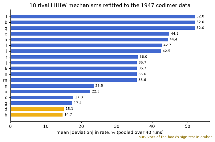
The data cannot separate the two surviving mechanisms. Pooled over the three temperatures, mechanism d fits to 15.1 % mean absolute deviation in rate and mechanism h to 14.7 % - a gap of 0.4 percentage points on a run-reproducibility floor the book itself puts at the same scale as the fit (“the experimental accuracy of individual runs is no better than this”). The sign at 200 C even favours h (15.1 vs 16.8 %), so the book’s stated ground that “the experimental fit is better with mechanism d” does not survive refitting in rate space - the choice of d rests, as the book’s second argument already had it, on chemistry (no dissociation needed), not statistics. The failure is structural, not a noise problem: noiseless rates generated from the fitted h are captured by mechanism d to 3.6 % over the same 12 compositions of the 200 C block - the two functional forms are too close over a 1-3.5 atm design to be told apart at any realistic precision. Kiani & Wachs (2024) make the same point about the pair-site content of these fits from the surface-science side.
But the field is not flat. The best rejected mechanism (desorption control, c/g) sits 2.7 points behind, mechanisms missing the product term cost real fit quality (dropping \(K_Sp_S\) from d degrades 200 C from 16.8 to 23.0 %), and the structurally wrong forms (no \(p_U\), no \(p_H\), or the uncatalysed \(r = kp_Hp_U\)) sit at 2-4x the deviation of d. So the printed data do discriminate the family shape - dual-site surface control with all three species adsorbed - while genuinely failing to resolve molecular vs atomic hydrogen. A well-established negative, measured on the formalism’s own founding dataset.
4. The temperature correlation, Table G, and the eq. (q) misprint
"""Reproduce the book's two-step temperature treatment and adjudicate dS_S."""
T3 = np.array([T_OF[t] for t in (200, 275, 325)])
exp_vals = {k: TG.loc[f"{k}_experimental"].to_numpy(float) for k in "abcf"}
corr_fit = {}
for k, v in exp_vals.items():
    slope, icept = np.polyfit(1 / T3, np.log(v), 1)
    corr_fit[k] = np.exp(icept + slope / T3)
corr_tbl = pd.DataFrame(
    {f"{k} {lab}": arr for k in "abcf"
     for lab, arr in (("(refit)", corr_fit[k]),
                      ("(printed)", TG.loc[f"{k}_corrected"].to_numpy(float)))},
    index=["200C", "275C", "325C"]).T
show(corr_tbl.style.format("{:.3f}").set_uuid("c1106"))
M["tableG_corrected_max_rel"] = float(max(
    np.max(np.abs(corr_fit[k] - TG.loc[f"{k}_corrected"].to_numpy(float))
           / TG.loc[f"{k}_corrected"].to_numpy(float)) for k in "abcf"))
# break test: regress ln(constant) against T instead of 1/T
wrongT = {}
for k, v in exp_vals.items():
    s2, i2 = np.polyfit(T3, np.log(v), 1)
    wrongT[k] = np.exp(i2 + s2 * T3)
bad_corr = float(max(
    np.max(np.abs(wrongT[k] - TG.loc[f"{k}_corrected"].to_numpy(float))
           / TG.loc[f"{k}_corrected"].to_numpy(float)) for k in "abcf"))
BREAKS.append(("tableG_corrected_max_rel", f"{M['tableG_corrected_max_rel']:.1e}",
               "lines fitted vs T instead of 1/T", f"{bad_corr:.2f}", "moves"))

# derived K rows - computed from the PRINTED corrected constants, so this
# checks the book's eq. (n) arithmetic, not our line fits
ap, bp, cp, fp = (TG.loc[f"{k}_corrected"].to_numpy(float) for k in "abcf")
derived = {"K_U": bp/ap, "K_S": cp/ap, "K_H": fp/ap,
           "alpha_Ek": 1/(ap**2*(fp/ap)*(bp/ap))}
M["tableG_derived_K_max_rel"] = float(max(
    np.max(np.abs(v - TG.loc[k].to_numpy(float)) / TG.loc[k].to_numpy(float))
    for k, v in derived.items()))
swap_dev = float(np.max(np.abs(fp/ap - TG.loc["K_U"].to_numpy(float))
                        / TG.loc["K_U"].to_numpy(float)))
BREAKS.append(("tableG_derived_K_max_rel", f"{M['tableG_derived_K_max_rel']:.1e}",
               "swap the K_U and K_H relations (K_U = f/a)",
               f"{swap_dev:.2f}", "moves; note this metric checks the book's "
               "eq. (n) arithmetic only - it shares the printed corrected "
               "constants with Table G, so it cannot fail for a bad line fit"))

# van 't Hoff constants from the PRINTED K rows (the book's own step)
vh = {}
for key in ("K_U", "K_S", "K_H", "alpha_Ek"):
    slope, icept = np.polyfit(1 / T3, np.log(TG.loc[key].to_numpy(float)), 1)
    vh[key] = (-slope * RGAS, icept * RGAS)          # (dH, dS) / (A, B)
vh_tbl = pd.DataFrame({
    "refit dH (or A)": {k: v[0] for k, v in vh.items()},
    "refit dS (or B)": {k: v[1] for k, v in vh.items()},
    "printed dH": {"K_U": TH["dH_U"], "K_S": TH["dH_S"], "K_H": TH["dH_H"],
                   "alpha_Ek": -TH["A"]},
    "printed dS": {"K_U": TH["dS_U"], "K_S": TH["dS_S"], "K_H": TH["dS_H"],
                   "alpha_Ek": TH["B"]}})
show(vh_tbl.style.format("{:.2f}").set_uuid("c1107"))

# adjudication: which printed dS_S reproduces the printed K_S row?
KS_row = TG.loc["K_S"].to_numpy(float)
KS_from = lambda dss: np.exp(-TH["dH_S"] / (RGAS * T3) + dss / RGAS)
rms = lambda dss: float(np.sqrt(np.mean(((KS_from(dss) - KS_row) / KS_row) ** 2)))
M["KS_row_rms_rel_tableG_dSS"] = rms(TH["dS_S"])       # -30.46
M["KS_row_rms_rel_eqq_dSS"]    = rms(TH["dS_S_eqq"])   # -30.96
BREAKS.append(("KS_row_rms_rel_tableG_dSS", f"{M['KS_row_rms_rel_tableG_dSS']:.1e}",
               "use eq. (q)'s dS_S = -30.96 instead of Table G's -30.46",
               f"{M['KS_row_rms_rel_eqq_dSS']:.1e}",
               "moves 10x: the adjudication is its own break test"))

display(Markdown(f"""
The corrected constants refit to within
**{M["tableG_corrected_max_rel"]:.1%}** of Table G (worst at 200 C - the
book's hand-fitted lines), and the derived $K$ rows close to
**{M["tableG_derived_K_max_rel"]:.1%}**, confirming the printed relations
$K_U = b/a$, $K_S = c/a$, $K_H = f/a$, $\\alpha = 1/(a^2K_HK_U)$.

**The misprint, adjudicated.** With the printed $\\Delta H_S = -13{{,}}700$,
Table G's $\\Delta S_S = -30.46$ reproduces the printed $K_S$ row (0.489,
0.0646, 0.0222) to **{M["KS_row_rms_rel_tableG_dSS"]:.1%}** rms; eq. (q)'s
$-30.96$ misses the same row by **{M["KS_row_rms_rel_eqq_dSS"]:.1%}** - the
final boxed equation carries the typo, the table is right. An implementation
typed from the (more convenient) eq. (q) box inherits a $K_S$ about
{100 * (1 - float(np.exp((TH["dS_S_eqq"] - TH["dS_S"]) / RGAS))):.0f} % low.
The free refit of the $K_S$ row lands at $\\Delta S_S$ = {vh["K_S"][1]:.2f} -
numerically *between* the two printed values, so the intercept alone
adjudicates nothing; what settles it is the pair test above, where Table G's
$(\\Delta H, \\Delta S)$ reproduces the printed $K_S$ row at
{M["KS_row_rms_rel_tableG_dSS"]:.1%} rms against eq. (q)'s {M["KS_row_rms_rel_eqq_dSS"]:.1%}.
"""))| 200C | 275C | 325C | |
|---|---|---|---|
| a (refit) | 2.659 | 3.176 | 3.488 |
| a (printed) | 2.640 | 3.140 | 3.430 |
| b (refit) | 1.531 | 1.584 | 1.613 |
| b (printed) | 1.530 | 1.580 | 1.610 |
| c (refit) | 1.383 | 0.199 | 0.071 |
| c (printed) | 1.290 | 0.203 | 0.076 |
| f (refit) | 1.084 | 0.772 | 0.646 |
| f (printed) | 1.010 | 0.774 | 0.653 |
| refit dH (or A) | refit dS (or B) | printed dH | printed dS | |
|---|---|---|---|---|
| K_U | -958.71 | -3.11 | -940.00 | -3.08 |
| K_S | -13911.63 | -30.82 | -13700.00 | -30.46 |
| K_H | -3139.20 | -8.53 | -3110.00 | -8.49 |
| alpha_Ek | 1764.74 | 2.85 | -1740.00 | 2.82 |
The corrected constants refit to within 7.4% of Table G (worst at 200 C - the book’s hand-fitted lines), and the derived \(K\) rows close to 1.5%, confirming the printed relations \(K_U = b/a\), \(K_S = c/a\), \(K_H = f/a\), \(\alpha = 1/(a^2K_HK_U)\).
The misprint, adjudicated. With the printed \(\Delta H_S = -13{,}700\), Table G’s \(\Delta S_S = -30.46\) reproduces the printed \(K_S\) row (0.489, 0.0646, 0.0222) to 2.5% rms; eq. (q)’s \(-30.96\) misses the same row by 23.6% - the final boxed equation carries the typo, the table is right. An implementation typed from the (more convenient) eq. (q) box inherits a \(K_S\) about 22 % low. The free refit of the \(K_S\) row lands at \(\Delta S_S\) = -30.82 - numerically between the two printed values, so the intercept alone adjudicates nothing; what settles it is the pair test above, where Table G’s \((\Delta H, \Delta S)\) reproduces the printed \(K_S\) row at 2.5% rms against eq. (q)’s 23.6%.
"""Eq. (q) against all 40 measured rates, and the rate-maximum it implies."""
TT = A.temp_C.map(T_OF).to_numpy()
H, U, S, r = (A[k].to_numpy() for k in
              ("pH_atm", "pU_atm", "pS_atm", "r_lbmol_per_lb_hr"))
r_pred = rate_eqq(TT, H, U, S)
pct = 100 * np.abs(r_pred - r) / r
M["eqq_all40_mean_abs_pct"] = float(pct.mean())
per_T = {t: float(pct[A.temp_C == t].mean()) for t in (200, 275, 325)}

# the same comparison with the per-temperature linearised constants (Table G
# experimental row) - the book's +-8.44 % was in R = sqrt(pHpU/r) space:
a2, b2, c2, f2 = (TG.loc[f"{k}_experimental", "val_200C"] for k in "abcf")
H0, U0, S0, r0 = (A[A.temp_C == 200][k].to_numpy() for k in
                  ("pH_atm", "pU_atm", "pS_atm", "r_lbmol_per_lb_hr"))
r_lin = H0 * U0 / (a2 + f2*H0 + b2*U0 + c2*S0) ** 2
pct_r_space = float(np.mean(100 * np.abs(r_lin - r0) / r0))
M["rate_space_scatter_pct_200C"] = pct_r_space
M["rate_space_over_R_space_ratio"] = pct_r_space / M["tableC_avg_abs_pct"]

# rate maximum vs temperature at the run-3c composition (Fig. 189's claim)
Ts = np.linspace(380, 750, 3000)
rT = rate_eqq(Ts, 2.459, 0.527, 0.515)
M["rate_max_T_K_run3c_composition"] = float(Ts[np.argmax(rT)])
r_noads = rate_eqq(Ts, 2.459, 0.527, 0.515) * (
    1 + eqq_constants(Ts)[1]*2.459 + eqq_constants(Ts)[2]*0.527
      + eqq_constants(Ts)[3]*0.515) ** 2          # numerator alone
assert np.all(np.diff(r_noads) < 0), "numerator alone should fall monotonically"
BREAKS.append(("rate_max_T_K_run3c_composition",
               f"{M['rate_max_T_K_run3c_composition']:.0f}",
               "delete the adsorption group (numerator alone)",
               f"monotone decreasing over {Ts[0]:.0f}-{Ts[-1]:.0f} K, no "
               "interior maximum",
               "moves off-scale: the maximum exists only through the "
               "competition of numerator and adsorption group (the combined "
               "numerator dH is -2310 cal/mol, so it falls with T)"))

# defect injection on the global comparison
r_lin1 = rate_eqq(TT, H, U, S) * (1 + eqq_constants(TT)[1]*H + eqq_constants(TT)[2]*U
                                  + eqq_constants(TT)[3]*S)   # exponent 2 -> 1
pct_exp1 = float(np.mean(100 * np.abs(r_lin1 - r) / r))
pct_eqq_dss = float(np.mean(100 * np.abs(rate_eqq(TT, H, U, S, dS_S=TH["dS_S_eqq"]) - r) / r))
BREAKS.append(("eqq_all40_mean_abs_pct", f"{M['eqqq' if False else 'eqq_all40_mean_abs_pct']:.1f}",
               "adsorption-group exponent 2 -> 1",
               f"{pct_exp1:.1f}", "moves: the dual-site exponent is load-bearing"))
BREAKS.append(("eqq_all40_mean_abs_pct", f"{M['eqq_all40_mean_abs_pct']:.1f}",
               "eq. (q)'s dS_S misprint (-30.96)",
               f"{pct_eqq_dss:.1f}",
               "barely moves: K_S p_S is a small denominator term, so THIS "
               "metric cannot adjudicate the misprint - the K_S row check above can"))

display(Markdown(f"""
**The final correlation against the data it came from:** eq. (q) (with Table
G's $\\Delta S_S$) reproduces the 40 measured rates to
**{M["eqq_all40_mean_abs_pct"]:.1f} %** mean absolute deviation
({per_T[200]:.1f} / {per_T[275]:.1f} / {per_T[325]:.1f} % at 200 / 275 /
325 C). That is *worse* than the book's famous +-8.44 % for two reasons this
page separates: the 8.44 is in the transformed variable
$R \\propto 1/\\sqrt{{r}}$, so it corresponds to about
**{M["rate_space_scatter_pct_200C"]:.1f} %** in the rate itself
({M["rate_space_over_R_space_ratio"]:.2f}x, at 200 C with the book's own
constants - the delta-method factor of 2 for a square root, measured); and
eq. (q) smooths the three per-temperature fits through the van 't Hoff lines,
paying a further few points for consistency in $T$. Both numbers are
*fit-quality on fitting data*, not validation - the source contains no
held-out measurement.

**The retardation the book makes so much of is real in its own constants:**
at run 3c's composition, eq. (q)'s rate peaks at
**{M["rate_max_T_K_run3c_composition"]:.0f} K
({M["rate_max_T_K_run3c_composition"] - 273.16:.0f} C)** - inside the
experimental window and far below the ~650 K reversibility threshold, exactly
the adsorption-starvation maximum Fig. 189 draws (computed here from printed
constants; the figure itself was never digitised).
"""))

# parity plot: fixed per-temperature colors + distinct markers (CVD-safe pairing)
fig, ax = plt.subplots(figsize=(5.4, 5.2))
style = {200: ("#4269d0", "o"), 275: ("#efb118", "s"), 325: ("#9c5bcd", "^")}
for t, (col, mk) in style.items():
    m = A.temp_C == t
    ax.plot(r[m], r_pred[m], mk, color=col, ms=6, mec="white", mew=0.5,
            label=f"{t} C")
lim = [0, 1.05 * max(r.max(), r_pred.max())]
ax.plot(lim, lim, "-", color="0.75", lw=1, zorder=0)
ax.plot(lim, [1.2 * x for x in lim], ":", color="0.85", lw=1, zorder=0)
ax.plot(lim, [x / 1.2 for x in lim], ":", color="0.85", lw=1, zorder=0)
ax.set_xlabel("measured rate, lb-mol/(hr lb cat)")
ax.set_ylabel("eq. (q) rate, lb-mol/(hr lb cat)")
ax.set_title("Final 1947 correlation vs its own 40 fitting runs\n(dotted: +-20 %)")
ax.legend(frameon=False)
ax.spines[["top", "right"]].set_visible(False)
ax.set_xlim(lim); ax.set_ylim(lim)
plt.tight_layout(); plt.show()
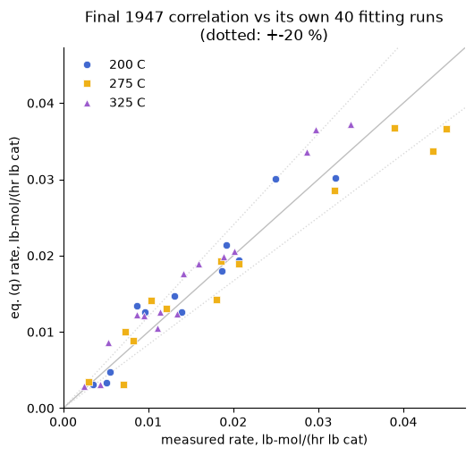
The final correlation against the data it came from: eq. (q) (with Table G’s \(\Delta S_S\)) reproduces the 40 measured rates to 19.1 % mean absolute deviation (17.8 / 19.2 / 19.9 % at 200 / 275 / 325 C). That is worse than the book’s famous +-8.44 % for two reasons this page separates: the 8.44 is in the transformed variable \(R \propto 1/\sqrt{r}\), so it corresponds to about 16.9 % in the rate itself (2.00x, at 200 C with the book’s own constants - the delta-method factor of 2 for a square root, measured); and eq. (q) smooths the three per-temperature fits through the van ’t Hoff lines, paying a further few points for consistency in \(T\). Both numbers are fit-quality on fitting data, not validation - the source contains no held-out measurement.
The retardation the book makes so much of is real in its own constants: at run 3c’s composition, eq. (q)’s rate peaks at 579 K (306 C) - inside the experimental window and far below the ~650 K reversibility threshold, exactly the adsorption-starvation maximum Fig. 189 draws (computed here from printed constants; the figure itself was never digitised).
5. The fitted law in a bed: a pymrm plug-flow demonstration
Chapter XXI poses exactly this problem (its Problem 1: isothermal bed, pure codimer feed, hydrogen 40 per cent over stoichiometric, 99.8 per cent hydrogenation, using “the nickel catalyst of Illustration 2”) but at 250-350 F - below the temperature range of the constants - and prints no answer. The demonstration therefore runs at 200 C and 3.5 atm, inside the fitted range, with the bed properties of the book’s own specimen run 3c. It is labelled a demonstration: no printed target exists.
Two independent routes: the pymrm finite-volume column (upwind convection of the three molar fluxes in catalyst-mass coordinate, Newton with a NumJac((n, 3)) pointwise-coupled stencil), and a gridless quadrature of the design equation \(\mathrm{d}X/\mathrm{d}(W/F_{U0}) = r(X)\). They share the rate function - so their agreement tests the transport discretisation and nothing about the rate law - and they share nothing else.
"""Plug-flow bed at 200 C, 3.5 atm: W/F for 99.8 % hydrogenation.

U + H2 -> S removes one mole per mole converted: total molar flow falls from
2.4 to 1.402 per mole of U fed (-42 %), and the partial pressures must follow
the LOCAL total. The naive fixed-total variant is the classic silent error
(the F2.3 lesson in mole-flow form) and is measured below."""
from scipy.integrate import solve_ivp
from scipy.interpolate import interp1d
from pymrm import construct_convflux_upwind, construct_div, NumJac, newton

T_K, PI = T_OF[200], 3.5
AL, KH, KU, KS = eqq_constants(T_K)
def rate_local(pHl, pUl, pSl):
    return AL * KH * KU * pHl * pUl / (1 + KH*pHl + KU*pUl + KS*pSl) ** 2

N_IN = np.array([1.0, 1.4, 0.0])      # U, H2, S per (lb-mol U/hr); 40 % excess H2
NU_STOICH = np.array([-1.0, -1.0, 1.0])
X_TARGET = 0.998

# ---- route 1: gridless quadrature in conversion space ----------------------
def dXdW(w, X, moving_total=True):
    nU, nH, nS = 1 - X[0], 1.4 - X[0], X[0]
    ntot = (nU + nH + nS) if moving_total else 2.4
    return [rate_local(PI*nH/ntot, PI*nU/ntot, PI*nS/ntot)]
ev = lambda w, X: X[0] - X_TARGET; ev.terminal = True
sol = solve_ivp(dXdW, [0, 5000], [0.0], rtol=1e-11, atol=1e-13, events=ev)
W_quad = float(sol.t_events[0][0])
sol0 = solve_ivp(lambda w, X: dXdW(w, X, False), [0, 5000], [0.0],
                 rtol=1e-11, atol=1e-13, events=ev)
W_naive = float(sol0.t_events[0][0])
M["reactor_WF_998_quadrature"] = W_quad
M["reactor_naive_fixed_total_bias_rel"] = (W_naive - W_quad) / W_quad

# ---- route 2: pymrm finite-volume column -----------------------------------
def pymrm_column(n, w_end, moving_total=True, nu_geom=0,
                 out_bc={"a": 1.0, "b": 0.0, "d": 0.0}):
    """Steady d(N_i)/dw = nu_i * r with unit convective velocity in w."""
    w_f = np.linspace(0.0, w_end, n + 1)
    w_c = 0.5 * (w_f[:-1] + w_f[1:])
    # inlet: N = N_IN (Dirichlet); outlet: zero outward gradient (outflow).
    bc = ({"a": 0.0, "b": 1.0, "d": N_IN[None, :]}, out_bc)
    conv, conv_bc = construct_convflux_upwind((n, 3), w_f, w_c, bc, v=1.0)
    div = construct_div((n, 3), w_f, nu=nu_geom)   # nu=0: mass coordinate, Cartesian
    L = div @ conv
    bvec = np.asarray((div @ conv_bc).todense()).ravel()
    jac = NumJac((n, 3))                            # fields on the LAST axis
    def src(Nflat):
        N = np.clip(Nflat.reshape(n, 3), 1e-14, None)
        ntot = N.sum(axis=1) if moving_total else np.full(n, N_IN.sum())
        p = PI * N / ntot[:, None]
        return NU_STOICH[None, :] * rate_local(p[:, 1], p[:, 0], p[:, 2])[:, None]
    def fun(Nflat):
        s, ds = jac(lambda x: src(x), Nflat)
        return (L @ Nflat + bvec) - s.ravel(), L - ds
    res = newton(fun, np.tile(N_IN, (n, 1)).ravel(), tol=1e-12, maxfev=50)
    assert res.success, "Newton did not converge"     # assert, never infer
    N = res.x.reshape(n, 3)
    X = 1 - N[:, 0] / N_IN[0]
    return w_c, X, N

W_grid, orders = {}, []
for n in (100, 200, 400, 800):
    w_c, X, N = pymrm_column(n, 140.0)
    W_grid[n] = float(interp1d(X, w_c)(X_TARGET))
for n0, n1 in ((100, 200), (200, 400), (400, 800)):
    e0, e1 = W_grid[n0] - W_quad, W_grid[n1] - W_quad
    orders.append(np.log2(e0 / e1))
W_rich = 2 * W_grid[800] - W_grid[400]              # Richardson, first order
M["reactor_WF_two_routes_rel_n800"]   = abs(W_grid[800] - W_quad) / W_quad
M["reactor_WF_richardson_vs_quad_rel"] = abs(W_rich - W_quad) / W_quad
M["reactor_observed_order"]            = float(np.mean(orders))

# total-flow contraction along the bed, and the profile figure
w_c, X, N = pymrm_column(400, 140.0)
contraction = N.sum(axis=1) / N_IN.sum()
M["reactor_total_flow_contraction"] = float(1 - contraction.min())

# ---- defect injections on the reactor --------------------------------------
w_cn, Xn, _ = pymrm_column(400, 250.0, moving_total=False)
W_naive_grid = float(interp1d(Xn, w_cn)(X_TARGET))
BREAKS.append(("reactor_WF_two_routes_rel_n800",
               f"{M['reactor_WF_two_routes_rel_n800']:.1e}",
               "partial pressures from the FIXED inlet total (no contraction)",
               f"{abs(W_naive_grid - W_quad)/W_quad:.2f}",
               "moves 2 orders: the mole-change term is worth half the bed"))
import warnings
try:
    with warnings.catch_warnings():
        warnings.simplefilter("ignore")
        pymrm_column(100, 140.0, out_bc={"a": 0.0, "b": 1.0, "d": 0.0})
    bad_bc = "converged (wrong answer)"
except (AssertionError, ValueError):
    bad_bc = "Jacobian exactly singular; Newton returns NaN"
BREAKS.append(("reactor_WF_two_routes_rel_n800", "-",
               "outlet forced Dirichlet N=0 instead of outflow", bad_bc,
               "the F2.3 outlet trap in reverse: with upwind convection the "
               "outlet value multiplies nothing, so pinning it removes a "
               "usable equation and the matrix goes singular - loudly here, "
               "silently when the row is merely left out"))
try:
    w_cg, Xg, _ = pymrm_column(400, 140.0, nu_geom=1)
    W_wrong_nu = float(interp1d(Xg, w_cg)(X_TARGET))
    nu_row = f"{abs(W_wrong_nu - W_quad)/W_quad:.2f}"
except (AssertionError, ValueError):
    nu_row = "Newton fails to converge (1/w singularity at the inlet face)"
BREAKS.append(("reactor_WF_two_routes_rel_n800", "-",
               "construct_div with nu=1 (cylindrical) in a mass coordinate",
               nu_row, "geometry factor is not decoration"))

display(Markdown(f"""
**W/F for 99.8 % hydrogenation at 200 C, 3.5 atm:
{W_quad:.1f} lb cat (lb-mol U/hr)^-1** by quadrature;
the pymrm column converges onto it at first order (observed
{M["reactor_observed_order"]:.2f}), {W_grid[800]:.1f} at n = 800
({M["reactor_WF_two_routes_rel_n800"]:.1e} relative) and
{W_rich:.1f} Richardson-extrapolated
({M["reactor_WF_richardson_vs_quad_rel"]:.1e}). With run 3c's bed density
(86.4 lb/ft3) and cross-section (0.00601 ft2), that is a bed of
{W_quad * 0.00904 / (86.4 * 0.00601):.2f} ft for run 3c's feed rate.

**The contraction is not a refinement.** Total molar flow falls
{M["reactor_total_flow_contraction"]:.0%} across the bed; holding the total at
its inlet value - a one-line slip that produces a perfectly smooth, plausible
profile - lengthens the required bed by
**{M["reactor_naive_fixed_total_bias_rel"]:.0%}**. The book's own Chapter XXI
material balance (Table LXI) is precisely this bookkeeping, done by hand.
"""))

fig, axes = plt.subplots(1, 2, figsize=(9.6, 4.0))
ax = axes[0]
ax.plot(w_c, X, color="#4269d0", lw=2, label="moving total (correct)")
ax.plot(w_cn[w_cn <= 250], Xn[w_cn <= 250], color="#9c5bcd", lw=2, ls="--",
        label="fixed inlet total (naive)")
ax.axhline(X_TARGET, color="0.8", lw=1, zorder=0)
ax.set_xlabel(r"$w = W/F_{U0}$, lb cat (lb-mol U/hr)$^{-1}$")
ax.set_ylabel("conversion of codimer, X")
ax.legend(frameon=False, loc="lower right")
ax.spines[["top", "right"]].set_visible(False)
ax = axes[1]
ax.plot(w_c, contraction, color="#4269d0", lw=2)
ax.set_xlabel(r"$w = W/F_{U0}$")
ax.set_ylabel("total molar flow / inlet value")
ax.spines[["top", "right"]].set_visible(False)
fig.suptitle("Eq. (q) in an isothermal bed at 200 C, 3.5 atm - a demonstration, "
             "no printed target exists", fontsize=10)
plt.tight_layout(); plt.show()
W/F for 99.8 % hydrogenation at 200 C, 3.5 atm: 106.6 lb cat (lb-mol U/hr)^-1 by quadrature; the pymrm column converges onto it at first order (observed 0.99), 107.1 at n = 800 (4.4e-03 relative) and 106.6 Richardson-extrapolated (1.6e-05). With run 3c’s bed density (86.4 lb/ft3) and cross-section (0.00601 ft2), that is a bed of 1.86 ft for run 3c’s feed rate.
The contraction is not a refinement. Total molar flow falls 42% across the bed; holding the total at its inlet value - a one-line slip that produces a perfectly smooth, plausible profile - lengthens the required bed by 51%. The book’s own Chapter XXI material balance (Table LXI) is precisely this bookkeeping, done by hand.
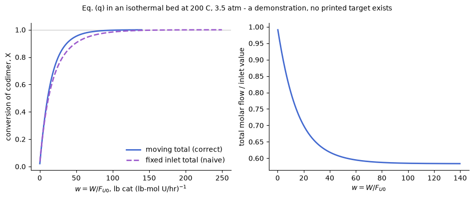
Validation
Everything numbered on this page is checked by one of four kinds of evidence, and every reported metric has a break row - a deliberate defect that moves it - or is labelled with what it cannot detect:
- printed checksums - the book’s own sums prove the 200 C transcription;
- printed intermediates - normal equations, eliminated system, solution, \(\Sigma\delta^2\), the +-8.44, Tables C-G;
- two-route computations - constants from transcribed data vs from the book’s printed sums; W/F from a pymrm grid vs a gridless quadrature; the corrupted-worksheet value from two independent printed rows;
- the adjudications - each printed inconsistency (25a, the \(\Delta S_S\) misprint, the duplicate-row disagreements) is decided by the book’s own adjacent numbers, never by preference.
What the break table cannot see, stated plainly: the two reactor routes share the rate function, so their agreement can never catch an error in eq. (q) itself (the eq. (q)-vs-data comparison and the K-row reproductions carry that load); the 275/325 transcriptions have no printed checksum, so a transcription slip there is only caught if it disturbs the Table E/F reproduction beyond the book’s own rounding; and no perturbation can detect that all comparisons stand on the same 40 runs - there is no independent measurement anywhere in this source, which is why every agreement above is labelled reproduction, not validation.
"""Break table and agreement metrics."""
bt = pd.DataFrame(BREAKS, columns=["metric", "healthy", "injected defect",
                                   "with defect", "verdict"])
show(bt.style.hide(axis="index").set_uuid("c1108"))

display(Markdown("""
**Structural / labelled rows** (kept, with what they are):

- `tableA_linear_psum_max_abs` sits at machine precision and **below
  check_agreement.py's ABS_FLOOR = 1e-12**, so CI does not regression-protect
  it; it is published as the record of an exact reproduction, and its break
  row above shows it moves under a single-digit slip.
  `tableA_product_psum_max_rel` has the book's own 3-4-decimal rounding as its
  floor and moves under the same slip.
- `DEF_verdict_flips_thr5pct` and `DEF_joint_acceptable_set_size` are counts
  from the threshold sweep; the sweep itself is their break row. The honest
  content is the pair: per-table verdicts are threshold-sensitive at 325 C,
  the joint decision is not.
- `rate_space_over_R_space_ratio` is close to 2 *by construction* for small
  errors (delta method on a square root); it is reported to quantify how far
  the printed +-8.44 % understates rate-space scatter, not as an independent
  agreement. `rate_space_scatter_pct_200C` is the fit-quality number that
  ratio is built on and inherits the Table C break rows (any refit-moving
  defect moves it).
- `run3c_specimen_rate_vs_tableA_rel` records the book's own unexplained
  0.7 % normalisation between its specimen arithmetic and its data table.
- `nls_h_mean_abs_pct_pooled` breaks the same way as the d row (its terms are
  the same three species); no separate injection is run.
- `reactor_observed_order` is the diagnostic on the grid study itself; the
  expected value for bare upwind is 1, and the naive/nu/bc rows all run
  through the same solve, so a broken discretisation shows here first.
- `reactor_total_flow_contraction` is stoichiometric arithmetic once the
  target conversion is reached (1 mole lost per mole converted from a feed of
  2.4): structural, kept as the record of the magnitude that makes the naive
  row expensive.
- `reactor_WF_998_quadrature` (the headline W/F) is covered by the naive,
  outlet-BC and nu rows and by the two-route comparison; it is a
  demonstration number with no printed target, as the section says.
- `discrim_third_best_gap_pct_points` inherits the power study and the K_S
  deletion row: both show what moves the family separation.
"""))

report_agreement("C1.1", M)| metric | healthy | injected defect | with defect | verdict |
|---|---|---|---|---|
| tableA_linear_psum_max_abs | 1.8e-15 | transcribe run 10a pS as 2.583 for 2.538 | 4.5e-02 | moves |
| tableA_Rsum_check_max_rel | 2.9e-03 | same single-digit slip | 9.5e-03 | moves |
| tableC_sum_delta_sq_rel_dev | 1.4e-03 | 10a pS digit slip, whole fit re-run | 4.8e-03 | moves |
| tableC_avg_abs_pct | 8.42 | same slip | 8.45 | moves |
| mechd_200C_vs_printed_max_rel | 5.8e-03 | same slip | 1.6e-02 | moves |
| mechd_200C_two_routes_max_rel | 6.3e-03 | route i run with the 10a digit slip (2.583 for 2.538) | 1.5e-02 | moves: route ii is immune to transcription, so the routes split |
| DEF_clean_rows_worst_rel_rhs | 1.7e-02 | mechanism h regressed on pH instead of sqrt(pH) (275 C) | 0.08 | moves: h's row (clean at 275 C) stops being explainable |
| DEF_corrupted_sum_two_witness_gap_rel | 1.1e-02 | attribute the corruption to Sum(R pU) instead of Sum(R pS) | 0.92 | cross-check fails: the two witnesses no longer agree |
| DEF_joint_acceptable_set_size | 2 = {d, h} | threshold swept 1-10 % (the knob the book's eyeball test hides) | unchanged; per-table flips go 0 -> 2 | the joint decision is threshold-robust, the per-table ones are not |
| nls_d_mean_abs_pct_pooled | 15.1 | delete the K_S pS term from mechanism d (200 C refit) | 23.0 | moves: the product-inhibition signal is real |
| discrim_d_vs_h_gap_pct_points | 0.4 | fit d to NOISELESS synthetic rates generated from the fitted h (numerical power study, clearly not data) | 3.6 | even exact h-rates are captured by d to a few %, far below the run scatter - the non-discrimination is structural to this design, not an artefact of noise |
| tableG_corrected_max_rel | 7.4e-02 | lines fitted vs T instead of 1/T | 0.16 | moves |
| tableG_derived_K_max_rel | 1.5e-02 | swap the K_U and K_H relations (K_U = f/a) | 0.59 | moves; note this metric checks the book's eq. (n) arithmetic only - it shares the printed corrected constants with Table G, so it cannot fail for a bad line fit |
| KS_row_rms_rel_tableG_dSS | 2.5e-02 | use eq. (q)'s dS_S = -30.96 instead of Table G's -30.46 | 2.4e-01 | moves 10x: the adjudication is its own break test |
| rate_max_T_K_run3c_composition | 579 | delete the adsorption group (numerator alone) | monotone decreasing over 380-750 K, no interior maximum | moves off-scale: the maximum exists only through the competition of numerator and adsorption group (the combined numerator dH is -2310 cal/mol, so it falls with T) |
| eqq_all40_mean_abs_pct | 19.1 | adsorption-group exponent 2 -> 1 | 90.2 | moves: the dual-site exponent is load-bearing |
| eqq_all40_mean_abs_pct | 19.1 | eq. (q)'s dS_S misprint (-30.96) | 19.5 | barely moves: K_S p_S is a small denominator term, so THIS metric cannot adjudicate the misprint - the K_S row check above can |
| reactor_WF_two_routes_rel_n800 | 4.4e-03 | partial pressures from the FIXED inlet total (no contraction) | 0.52 | moves 2 orders: the mole-change term is worth half the bed |
| reactor_WF_two_routes_rel_n800 | - | outlet forced Dirichlet N=0 instead of outflow | Jacobian exactly singular; Newton returns NaN | the F2.3 outlet trap in reverse: with upwind convection the outlet value multiplies nothing, so pinning it removes a usable equation and the matrix goes singular - loudly here, silently when the row is merely left out |
| reactor_WF_two_routes_rel_n800 | - | construct_div with nu=1 (cylindrical) in a mass coordinate | Newton fails to converge (1/w singularity at the inlet face) | geometry factor is not decoration |
Structural / labelled rows (kept, with what they are):
tableA_linear_psum_max_abssits at machine precision and below check_agreement.py’s ABS_FLOOR = 1e-12, so CI does not regression-protect it; it is published as the record of an exact reproduction, and its break row above shows it moves under a single-digit slip.tableA_product_psum_max_relhas the book’s own 3-4-decimal rounding as its floor and moves under the same slip.DEF_verdict_flips_thr5pctandDEF_joint_acceptable_set_sizeare counts from the threshold sweep; the sweep itself is their break row. The honest content is the pair: per-table verdicts are threshold-sensitive at 325 C, the joint decision is not.rate_space_over_R_space_ratiois close to 2 by construction for small errors (delta method on a square root); it is reported to quantify how far the printed +-8.44 % understates rate-space scatter, not as an independent agreement.rate_space_scatter_pct_200Cis the fit-quality number that ratio is built on and inherits the Table C break rows (any refit-moving defect moves it).run3c_specimen_rate_vs_tableA_relrecords the book’s own unexplained 0.7 % normalisation between its specimen arithmetic and its data table.nls_h_mean_abs_pct_pooledbreaks the same way as the d row (its terms are the same three species); no separate injection is run.reactor_observed_orderis the diagnostic on the grid study itself; the expected value for bare upwind is 1, and the naive/nu/bc rows all run through the same solve, so a broken discretisation shows here first.reactor_total_flow_contractionis stoichiometric arithmetic once the target conversion is reached (1 mole lost per mole converted from a feed of 2.4): structural, kept as the record of the magnitude that makes the naive row expensive.reactor_WF_998_quadrature(the headline W/F) is covered by the naive, outlet-BC and nu rows and by the two-route comparison; it is a demonstration number with no printed target, as the section says.discrim_third_best_gap_pct_pointsinherits the power study and the K_S deletion row: both show what moves the family separation.
Agreement metrics for C1.1:
  run3c_specimen_rate_vs_tableA_rel     = 0.0067144
  tableA_linear_psum_max_abs            = 1.7764e-15
  tableA_product_psum_max_rel           = 8.5263e-05
  tableA_Rsum_check_max_rel             = 0.0029421
  mechd_200C_vs_printed_max_rel         = 0.005764
  mechd_200C_two_routes_max_rel         = 0.0062971
  tableC_sum_delta_sq_rel_dev           = 0.0013759
  tableC_avg_abs_pct                    = 8.4239
  tableC_25a_printed_minus_consistent   = 0.5
  DEF_clean_rows_worst_rel_rhs          = 0.016889
  DEF_clean_row_count                   = 38
  DEF_corrupted_sum_two_witness_gap_rel = 0.010879
  DEF_verdict_flips_thr5pct             = 2
  DEF_joint_acceptable_set_size         = 2
  nls_d_mean_abs_pct_pooled             = 15.083
  nls_h_mean_abs_pct_pooled             = 14.72
  discrim_d_vs_h_gap_pct_points         = 0.36297
  discrim_third_best_gap_pct_points     = 2.6825
  discrim_power_d_fits_exact_h_pct      = 3.5828
  tableG_corrected_max_rel              = 0.073595
  tableG_derived_K_max_rel              = 0.014801
  KS_row_rms_rel_tableG_dSS             = 0.025087
  KS_row_rms_rel_eqq_dSS                = 0.23556
  eqq_all40_mean_abs_pct                = 19.05
  rate_space_scatter_pct_200C           = 16.856
  rate_space_over_R_space_ratio         = 2.001
  rate_max_T_K_run3c_composition        = 579.25
  reactor_WF_998_quadrature             = 106.62
  reactor_naive_fixed_total_bias_rel    = 0.50584
  reactor_WF_two_routes_rel_n800        = 0.0043721
  reactor_WF_richardson_vs_quad_rel     = 1.6482e-05
  reactor_observed_order                = 0.9945
  reactor_total_flow_contraction        = 0.41652
{'page': 'C1.1',
'metrics': {'run3c_specimen_rate_vs_tableA_rel': 0.006714429325819921,
'tableA_linear_psum_max_abs': 1.7763568394002505e-15,
'tableA_product_psum_max_rel': 8.526277104006247e-05,
'tableA_Rsum_check_max_rel': 0.002942058165548228,
'mechd_200C_vs_printed_max_rel': 0.005764036582206753,
'mechd_200C_two_routes_max_rel': 0.0062970782051921656,
'tableC_sum_delta_sq_rel_dev': 0.001375900414576228,
'tableC_avg_abs_pct': 8.423939077225173,
'tableC_25a_printed_minus_consistent': 0.4999999999999991,
'DEF_clean_rows_worst_rel_rhs': 0.016889329318868336,
'DEF_clean_row_count': 38.0,
'DEF_corrupted_sum_two_witness_gap_rel': 0.010879473723519958,
'DEF_verdict_flips_thr5pct': 2.0,
'DEF_joint_acceptable_set_size': 2.0,
'nls_d_mean_abs_pct_pooled': 15.083088647470042,
'nls_h_mean_abs_pct_pooled': 14.720120922353011,
'discrim_d_vs_h_gap_pct_points': 0.3629677251170307,
'discrim_third_best_gap_pct_points': 2.682544272759298,
'discrim_power_d_fits_exact_h_pct': 3.582793859957373,
'tableG_corrected_max_rel': 0.07359547857505681,
'tableG_derived_K_max_rel': 0.01480123220780295,
'KS_row_rms_rel_tableG_dSS': 0.02508653372684947,
'KS_row_rms_rel_eqq_dSS': 0.23556241457588617,
'eqq_all40_mean_abs_pct': 19.05029862048309,
'rate_space_scatter_pct_200C': 16.856047963757813,
'rate_space_over_R_space_ratio': 2.000969832430241,
'rate_max_T_K_run3c_composition': 579.2497499166388,
'reactor_WF_998_quadrature': 106.62273507467253,
'reactor_naive_fixed_total_bias_rel': 0.505843223787219,
'reactor_WF_two_routes_rel_n800': 0.004372059647938481,
'reactor_WF_richardson_vs_quad_rel': 1.6482052645927384e-05,
'reactor_observed_order': 0.9945029334100797,
'reactor_total_flow_contraction': 0.41652187946937747}}What pymrm adds
Honestly: the rate algebra needs no solver, and nothing in Sections 1-4 uses pymrm - that work is careful transcription, linear algebra and scipy.optimize, and its value is archival and statistical, not numerical. What this page adds over the book is (i) machine-precision proof of which printed numbers are right, (ii) the forensic identification of a single 1947 worksheet slip behind eight rows of Table D plus the misprint adjudication in eq. (q), and (iii) the modern answer to the discrimination question: the founding dataset supports the family (dual-site surface control, all three species adsorbed) but genuinely cannot resolve molecular vs atomic hydrogen - the book’s own stated fit-quality ground for choosing (d) does not survive refitting in rate space.
pymrm enters where the formalism meets a reactor: the Section 5 column is the S2 pattern every downstream LHHW page reuses - species on the last axis, NumJac((n, 3)) for a pointwise-coupled source, upwind convection with the outward-normal boundary convention, and the mole-contraction bookkeeping that the naive implementation silently drops at a measured cost of half the bed. This page is the formalism reference for C2.3 (ammonia synthesis), C2.4 (methanol), C2.10 (o-xylene) and C2.19 (ethanol dehydrogenation), each of which is an LHHW instance whose kinetic-term / driving-force / adsorption-group anatomy is defined here.
Reuse
- Take the rate law from Table G’s foot, not from eq. (q). The boxed final equation misprints \(\Delta S_S\) (\(-30.96\) for \(-30.46\)), which this page adjudicates from the book’s own \(K_S\) row; typing the box costs about 22 % of \(K_S\). The
eqq-thermodataset carries both printings, labelled. - Do not quote Tables D/E/F’s constants for the rejected mechanisms without this page’s forensics: at 200 C eight of the eighteen rows descend from one corrupted \(\Sigma R\,p_S\); three duplicate rows disagree with their printed siblings; the 275 C g/m row is unexplained arithmetic. The book’s decision survives: recomputed at full precision the joint acceptable set is still {d, h} at every threshold swept, though the per-table verdicts at 325 C are threshold-sensitive (Section 2).
- The famous +-8.44 % is in \(\sqrt{p_Hp_U/r}\), not in the rate. In rate space the same fit scatters about twice that; quote the space with the number.
- The constants are fit-range constants. 200-325 C, 1-3.5 atm, forward-only below ~650 K. Chapter XXI’s own Problem 1 asks for 250-350 F - already an extrapolation; eq. (q)’s adsorption enthalpies make the rate fall with temperature above about 580 K at mid-range compositions, so extrapolation errors are not sign-safe.
- In a bed, build partial pressures from the local total molar flow. The hydrogenation removes a mole per mole converted; holding the inlet total (a smooth, plausible-looking slip) lengthens the 99.8 %-conversion bed by half. Use the divergence form with
NumJac((n, 3))- never a bare(n,)shape, which builds a dense Jacobian. - Fit vs test: everything in the source is fitting data; there is no held-out measurement. A page that needs LHHW constants validated against independent data must look to the downstream instances (
C2.1is the model: 61 digitised held-out points), not to this book. - The two mechanism figures (Fig. 188a, Fig. 189) were never digitised; everything figure-shaped here is computed from printed constants. The Johanson-Watson toluene example (book pp. 959-961) is scoped out - its constants derive from conversion curves, a figure-digitisation route parked repo-wide.