# Bootstrap: the pymrm this page was checked with, and the gallery files it was
# published with. Works in a checkout, in CI and on a fresh Colab VM.
GALLERY_REF = "gallery-2026.11.10.3"  # replaced by the release tag at publication
PYMRM = ">=3.3.0,<4"  # equals meta.yaml pymrm_min_version, up to the next major
PAGE = "B3.1-shrinking-core"  # equals the page directory

import os, sys, urllib.request
from pathlib import Path
_shared = next((p / "shared" for p in (Path.cwd(), *Path.cwd().parents)
                if (p / "shared" / "gallery_bootstrap.py").is_file()), None)
if _shared is None:
    _shared = (Path(os.environ.get("XDG_CACHE_HOME") or Path.home() / ".cache")
               / "pymrm-gallery" / GALLERY_REF)
    _shared.mkdir(parents=True, exist_ok=True)
    urllib.request.urlretrieve(
        "https://raw.githubusercontent.com/computational-chemical-engineering/"
        f"pymrm-gallery/{GALLERY_REF}/shared/gallery_bootstrap.py",
        _shared / "gallery_bootstrap.py")
sys.path.insert(0, str(_shared))
sys.modules.pop("gallery_bootstrap", None)
from gallery_bootstrap import setup
setup(PAGE, PYMRM, GALLERY_REF); # the semicolon stops the cell echoing the pathThe shrinking core, and when its three textbook limits are safe to use
sec:B
struct:S12
tier:T0
data:tier6
phase:gas-solid
Yagi and Kunii’s one equation contains all three classical regimes. Reading it off the 1955 page and integrating the moving boundary independently gives the same thing to round-off, and then says where the simplifications may be used.
The shrinking core, and when its three textbook limits are safe to use
Catalog ID: B3.1 · Structures: S12 (moving boundary) · Tier: T0
A lump of carbon burning in air develops an ash shell. Oxygen must cross a boundary film, diffuse through that shell, and react at the surface of the shrinking unburned core. Three resistances in series, and a boundary that moves as the core is consumed.
Every textbook gives three limiting conversion-time laws for this problem, one per controlling resistance. Yagi and Kunii’s 1955 paper gives the single equation all three come from, and almost nobody quotes it.
# Imports. The page's model.py is put on sys.path by setup().
import numpy as np
import matplotlib.pyplot as plt
from IPython.display import Markdown, display
from pymrm.checks import observed_orders
from gallery_utils import Claims
from model import (LAWS, Shell, crest, eq6, flow_analytic, groups, limit_gaps, regime_map,
                   resistance_shares, theta_from_resistances)

plt.rcParams.update({"figure.dpi": 110, "axes.grid": True, "grid.alpha": 0.3})
claims = Claims(PAGE.split("-")[0])
BREAK = []   # (injected defect, claim, clean value, broken value, caught)


def brk(row, metric, broken):
    """One injected defect: ``broken`` is what claim ``metric`` becomes with it."""
    caught = claims.breaks(row, metric, broken)
    BREAK.append((row, metric, claims[metric], broken, caught))
    return caught
Background
The shrinking-core picture applies when the solid is non-porous: gas cannot penetrate the unreacted material, so reaction is confined to a sharp interface at radius \(r\) inside a particle of radius \(R\). Yagi and Kunii state the assumption directly: an ash layer “remains around the unburned core of the particle and prevents the diffusion of gas”.
The three resistances, and the three limiting laws they produce, are standard:
| controlling step | conversion-time law |
|---|---|
| gas film | \(\theta/\theta_B = X\) |
| ash-layer diffusion | \(\theta/\theta_B = 1 - 3(1-X)^{2/3} + 2(1-X)\) |
| surface reaction | \(\theta/\theta_B = 1 - (1-X)^{1/3}\) |
with \(X = 1 - (r/R)^3\) the conversion. What is not standard is that these are three corners of one expression, and that the paper prints it.
This page reproduces that expression, checks it two independent ways, and then answers the question the three-way split raises but never settles: given a real particle, which law may you actually use, and how wrong is it?
The published model
Two equations, read off 600 dpi renders of the printed page. The text layer of this scan is badly mangled (it renders \(\theta_B\) as 0B, \(\omega\) as ~, and Eq. 6’s numerator as a run of broken glyphs), so nothing here comes from OCR.
Eq. 5, the three resistances in series:
\[ \frac{1}{\bar k_1} = \frac{1}{k_{c1}} + \frac{1}{k_{d1}} + \frac{1}{3k_{f1}}, \qquad k_{d1} = \frac{12\,\mathbb{D}_{vs}}{D_p} \]
Note the factor 3 on the film term and the 12 in \(k_{d1}\). Both are easy to lose, and both are checkable; see the validation section.
Eq. 6, the position of the interface against time:
\[ \frac{\theta}{\theta_B} = 1 - \frac{\gamma\,(r/R) + 3\omega\gamma\,(r/R)^2 + \omega(1-2\gamma)\,(r/R)^3}{\omega + \omega\gamma + \gamma} \]
\[ \omega = \frac{k_{c1}}{k_{d1}},\qquad \gamma = \frac{3k_{f1}}{k_{d1}},\qquad \theta_B = \frac{D_p}{2\alpha\bar k_1 C_1} \]
\(\theta_B\) is the time for complete combustion. Two dimensionless groups \((\omega,\gamma)\) therefore fix the entire conversion history, which is why this page can be complete without a single physical property.
| symbol | code |
|---|---|
| \(\omega\), \(\gamma\) | omega, gamma of eq6; groups(kc, kf, D, R) builds them |
| \(r/R\) | x |
| \(k_{c1}\), \(k_{f1}\), \(\mathbb{D}_{vs}\), \(R = D_p/2\) | kc, kf, D, R |
Parameters and assumptions
Assumptions: non-porous solid, so a sharp interface; quasi-steady gas diffusion in the ash shell; constant particle size (ash retained, no shrinkage of the outer radius); isothermal; first-order in the gas.
What this page deliberately does not compute. The paper obtains \(k_{c1}\) in cm/s “by changing the unit of the specific combustion rate \(K_c\)” in Parker and Hottel’s correlation,
\[10^3 K_c = \frac{9.55\times10^{9}}{\sqrt{T}}\,P_o\,\exp(-44{,}000/RT),\]
but the unit conversion itself is not printed. Without it \(k_{c1}\) cannot be recovered, so no absolute burnout time is quoted anywhere below, and the paper’s Figure 6 is not reproduced. Guessing the conversion would put invented numbers on the page. Everything here is expressed in \(\omega\), \(\gamma\) and \(\theta/\theta_B\) instead, which is exactly what Eq. 6 needs and costs nothing: the physics of the regime question is entirely dimensionless.
The shell solves below need illustrative coefficients. Only their ratios matter, and the six cases span a thin and a thick shell with a slow reaction, a slow film and a slow ash layer.
R_P = 0.05    # particle radius (m), illustrative
D_G = 1e-4    # ash-layer diffusivity (m^2/s), illustrative
C_BULK = 1.0  # bulk concentration, normalised
# the six shell cases: (r_c/R, k_c, k_f) with k in m/s
CASES = [(xf, kc, kf) for xf in (0.9, 0.6, 0.3) for kc, kf in ((1e-2, 1e-2), (1.0, 1e-3))]
X_GRID = np.linspace(0, 1, 400)   # r/R for the history checks
The data
There is none, and there should not be. This page is provenance tier 6: the content is an analytic relation and its limits, and the checks below are mathematical rather than experimental. The paper’s own measurements are of fluidised-bed elutriation and particle size distributions, which belong to a different model entirely.
Recording that plainly matters more than it looks. The gallery’s rule is never to present a re-simulation as data; the honest alternative is to say that a page has no experimental content and to make its validation carry the weight instead.
PyMRM implementation
Three pieces. The first is the paper’s equation, the second is an independent route to it, and the third is the only part that needs a solver.
Eq. 6 directly. Two lines of algebra (eq6).
The moving boundary, integrated from the resistances. If Eq. 5 is right, then the instantaneous molar flow to a core at radius \(r_c\) is
\[ W = \frac{4\pi C_1}{\dfrac{1}{k_c r_c^2} + \dfrac{1}{\mathbb{D}}\left(\dfrac{1}{r_c}-\dfrac{1}{R}\right) + \dfrac{1}{k_f R^2}}, \]
and equating solid consumption to it gives \(\theta(r_c)\) by quadrature (theta_from_resistances). That route never looks at Eq. 6, so agreement between the two is a real check on having read the printed equation correctly.
The ash shell itself, with pymrm (Shell). The quasi-steady gas profile in \(r_c \le r \le R\) is a spherical diffusion problem with a Robin condition at each face, reaction at the inner one and film transfer at the outer:
\[ \nabla\!\cdot\!\left(-\mathbb{D}\nabla C\right) = 0,\qquad \left.\mathbb{D}\frac{\partial C}{\partial n} + k_c C\right|_{r_c}\!\!= 0,\qquad \left.\mathbb{D}\frac{\partial C}{\partial n} + k_f C\right|_{R}\!\!= k_f C_1 . \]
Both use the outward normal of the shell, which points inward at the core face. That is why the reaction condition has \(d = 0\) and the same sign structure as the film one. construct_div(..., nu=2) supplies the spherical geometry; the operators are assembled once in Shell.__init__.
Reading the flow. The molar flow to the core is \(4\pi r_c^2\,\mathbb{D}\,
\partial C/\partial r\) at the core face. compute_boundary_values returns that discrete gradient on the face with the shell’s own boundary dictionary, so the flow read is the one the solve conserves: each cell balances the flow through its two faces, so the flow through every face is the same number, the one the film delivers. The page states it as an identity and measures it.
shell = Shell(0.3 * R_P, R_P, D_G, 1e-2, 1e-2, n=400)
C = shell.solve()
print("shell:", shell.n, "cells,", "bc core face", shell.bc[0], "outer face", shell.bc[1])
print(f"flow to the core (face read) {shell.flow_core(C):.6e}, series resistance {flow_analytic(0.3*R_P, R_P, D_G, 1e-2, 1e-2):.6e}")
shell: 400 cells, bc core face {'a': 0.0001, 'b': 0.01, 'd': 0.0} outer face {'a': 0.0001, 'b': 0.01, 'd': 0.01}
flow to the core (face read) 1.321233e-05, series resistance 1.321231e-05Results
Eq. 6 against its own three corners, and against the independent integration.
x = X_GRID
X = 1 - x**3
BIG = 1e7    # omega of the ash limit
EPS = 1e-9   # gamma of the film limit and omega of the reaction limit
fig, ax = plt.subplots(1, 2, figsize=(12.2, 4.3))

for lab, f, col in (("film control", LAWS["film"], "tab:blue"),
                    ("ash-layer control", LAWS["ash"], "tab:green"),
                    ("reaction control", LAWS["reaction"], "tab:red")):
    ax[0].plot(X, f(X), lw=2.4, color=col, alpha=0.35, label=lab)
ax[0].plot(X, eq6(x, 1.0, EPS), "--", lw=1.4, color="tab:blue", label=r"eq. (6), $\gamma\to0$")
ax[0].plot(X, eq6(x, BIG, 3 * BIG), "--", lw=1.4, color="tab:green", label=r"eq. (6), $k_{d1}\to0$")
ax[0].plot(X, eq6(x, EPS, 1.0), "--", lw=1.4, color="tab:red", label=r"eq. (6), $\omega\to0$")
ax[0].set(xlabel="conversion $X$", ylabel=r"$\theta/\theta_B$", title="one equation, three corners")
ax[0].legend(fontsize=8, loc="lower right")

for om, ga, lab in ((0.05, 0.15, r"$\omega$=0.05, $\gamma$=0.15"),
                    (0.5, 1.0, r"$\omega$=0.5, $\gamma$=1"),
                    (5.0, 10.0, r"$\omega$=5, $\gamma$=10"),
                    (50.0, 100.0, r"$\omega$=50, $\gamma$=100")):
    ax[1].plot(X, eq6(x, om, ga), lw=1.9, label=lab)
ax[1].set(xlabel="conversion $X$", ylabel=r"$\theta/\theta_B$", title="and everything in between")
ax[1].legend(fontsize=8, loc="lower right")
fig.tight_layout(); plt.show()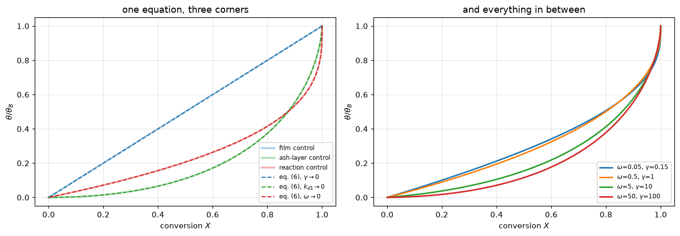
Validation
Four checks, and the first two are the ones that establish the printed equations were read correctly.
print("1. Eq. 6 is exact at both endpoints, for any (omega, gamma)")
PAIRS = [(0.3, 2.0), (5.0, 0.1), (1e3, 1e3), (1e-6, 1e6)]
for om, ga in PAIRS:
    print(f"   omega={om:9.1e} gamma={ga:9.1e}   theta(x=1) = {eq6(1.0, om, ga):+.2e}"
          f"   theta(x=0) = {eq6(0.0, om, ga):.10f}")
END_GAP = max(abs(eq6(1.0, om, ga)) for om, ga in PAIRS)
claims.bound("eq6_endpoint_x1", END_GAP, max=1e-14, basis="identity",
             note="the numerator at x = 1 equals the denominator term by term; round-off only")
brk("cubic coefficient read as omega (1 - gamma) (eq6(..., cubic='misread'))", "eq6_endpoint_x1",
    max(abs(eq6(1.0, om, ga, cubic="misread")) for om, ga in PAIRS))
print("   Nothing enforces this: the numerator at x=1 must collapse to the")
print("   denominator term by term, which it does only for the printed coefficients.\n")

print("2. Eq. 6 IS the integral of eq. 5's three resistances")
SIX = [(1e-2, 1e-2), (1e-1, 1e-3), (1e-3, 1e-1), (1.0, 1.0), (1e-4, 1e2), (1e2, 1e-4)]


def eq6_vs_integrated(**kw):
    """Largest difference of eq. 6 and the integrated resistances over the six cases."""
    worst = 0.0
    for kc, kf in SIX:
        om, ga = groups(kc, kf, D_G, R_P, **kw)
        worst = max(worst, float(np.abs(eq6(x, om, ga) - theta_from_resistances(x, kc, kf, D_G, R_P)).max()))
    return worst


print(f"   {'kc':>8}{'kf':>8}{'omega':>10}{'gamma':>10}{'max |diff|':>13}")
for kc, kf in SIX:
    om, ga = groups(kc, kf, D_G, R_P)
    d = np.abs(eq6(x, om, ga) - theta_from_resistances(x, kc, kf, D_G, R_P)).max()
    print(f"   {kc:8.0e}{kf:8.0e}{om:10.3f}{ga:10.3f}{d:13.2e}")
WORST6 = eq6_vs_integrated()
claims.bound("eq6_vs_integrated_worst", WORST6, max=1e-14, basis="identity",
             note="two closed forms of one function; round-off only")
brk("film term without the factor 3 (groups(..., film_factor=1))", "eq6_vs_integrated_worst",
    eq6_vs_integrated(film_factor=1.0))
brk("k_d1 = 6 D/D_p instead of 12 D/D_p (groups(..., kd_coef=6))", "eq6_vs_integrated_worst",
    eq6_vs_integrated(kd_coef=6.0))
_rat = [kc / kf for kc, kf in SIX]
print(f"   worst below 1e-14 (here {WORST6:.1e}) over {np.log10(max(_rat) / min(_rat)):.0f} decades of k_c/k_f.")
print("   The integration route never looks at eq. 6, and reproduces both the")
print("   factor 3 on the film term and the 12 in k_d1 = 12 D/D_p independently.\n")

print("3. Eq. 6 reduces to the three classical laws in their limits")
GAPS = limit_gaps(x, EPS, BIG, EPS)
claims.bound("eq6_to_film_limit", GAPS["film"], max=1e-9, basis="theory",
             note="the gap is proportional to gamma, with coefficient below 1")
claims.bound("eq6_to_ash_limit", GAPS["ash"], max=3e-8, basis="theory",
             note="the gap is proportional to 1/omega, with coefficient below 0.3")
claims.bound("eq6_to_reaction_limit", GAPS["reaction"], max=5e-10, basis="theory",
             note="the gap is proportional to omega, with coefficient below 0.5")
BAD = limit_gaps(x, 1e-5, 1e5, 1e-5)
for k in ("film", "ash", "reaction"):
    brk("limit parameters 1e-5 instead of 1e-9 (ash: omega = 1e5 instead of 1e7)", f"eq6_to_{k}_limit", BAD[k])


def scaling_dev(e1, e2):
    """Largest deviation of the limit gaps from proportionality to the small parameter."""
    a, b = limit_gaps(x, e1, 1 / e1, e1), limit_gaps(x, e2, 1 / e2, e2)
    return max(abs(np.log10(a[k] / b[k]) - np.log10(e1 / e2)) for k in a)


print(f"   {'small parameter':>16}{'film':>12}{'ash':>12}{'reaction':>12}")
for e in (1e-3, 1e-5, 1e-7, 1e-9):
    g = limit_gaps(x, e, 1 / e, e)
    print(f"   {e:16.0e}{g['film']:12.2e}{g['ash']:12.2e}{g['reaction']:12.2e}")
claims.bound("limit_gap_scaling_dev", scaling_dev(1e-5, 1e-9), max=1e-4, basis="theory",
             note="log10 of the gap ratio against log10 of the parameter ratio, 1e-5 against 1e-9")
brk("ladder 1e-1 and 1e-5: outside the linear range", "limit_gap_scaling_dev", scaling_dev(1e-1, 1e-5))
print("   each gap shrinks in proportion to its small parameter, so the corners are")
print("   limits of eq. (6), not approximations of it.\n")

print("4. The pymrm shell solve against the analytic series resistance")
NS = (25, 50, 100, 200, 400)


def shell_study(read="face", ns=NS, **kw):
    """Per case: error ladder of W / W_series, orders, conservation and read gaps at the finest grid."""
    out = []
    for xf, kc, kf in CASES:
        rc = xf * R_P
        Wa = flow_analytic(rc, R_P, D_G, kc, kf)

        def W(n):
            s = Shell(rc, R_P, D_G, kc, kf, n, **kw)
            return s.flow_core(s.solve(), read=read) / Wa

        o = observed_orders(W, ns)
        s = Shell(rc, R_P, D_G, kc, kf, ns[-1], **kw)
        Cf = s.solve()
        out.append({"xf": xf, "kc": kc, "kf": kf, "W": o["values"], "orders": o["orders"],
                    "err": abs(o["values"][-1] - 1.0),
                    "findiff": abs(o["values"][-1] - o["values"][-2]),
                    "cons": abs(s.flow_core(Cf) - s.flow_outer(Cf)) / Wa,
                    "face_gap": abs(s.flow_core(Cf) - s.flow_core(Cf, read="cells")) / Wa})
    return out


STUDY = shell_study()
print(f"   {'rc/R':>6}{'kc':>8}{'kf':>8}{'W pymrm':>13}{'W analytic':>13}{'rel err':>11}   orders on {NS[0]}..{NS[-1]} cells")
for r in STUDY:
    Wa = flow_analytic(r["xf"] * R_P, R_P, D_G, r["kc"], r["kf"])
    print(f"   {r['xf']:6.1f}{r['kc']:8.0e}{r['kf']:8.0e}{r['W'][-1]*Wa:13.5e}{Wa:13.5e}{r['err']:11.1e}"
          f"   {', '.join(f'{o:.2f}' for o in r['orders'])}")
WORST_ERR = max(r["err"] for r in STUDY)
claims.value("shell_solve_worst_rel_err", WORST_ERR)
claims.bound("shell_order_finest_min", min(r["orders"][-1] for r in STUDY), min=1.85, max=2.05, basis="theory",
             note="second-order scheme, approached from below on the thick shell (pre-asymptotic rungs)")
claims.bound("shell_order_finest_max", max(r["orders"][-1] for r in STUDY), min=1.85, max=2.05, basis="theory",
             note="as shell_order_finest_min")
claims.bound("shell_conservation_gap", max(r["cons"] for r in STUDY), max=1e-10, basis="identity",
             note="flow to the core against flow delivered by the film; round-off of the sparse solve, which grows with the grid")
claims.bound("shell_interior_face_gap", max(r["face_gap"] for r in STUDY), max=1e-12, basis="identity",
             note="the flow through the first interior face equals the core-face flow; round-off only")
RATIO = min(r["findiff"] / r["cons"] for r in STUDY)
claims.bound("shell_finest_over_roundoff", RATIO, min=1e3, basis="theory",
             note="finest difference of the ladder over the conservation gap, which is the round-off of the same solve")
print(f"\n   worst {WORST_ERR:.1e} at {NS[-1]} cells; the orders rise towards 2 on every case, as they should for a")
print("   second-order scheme still short of its asymptotic range on the thick shell.")
print(f"   conservation: flow to the core against the film flow, below 1e-10 (here {claims['shell_conservation_gap']:.1e});")
print(f"   first interior face against core face, below 1e-12 (here {claims['shell_interior_face_gap']:.1e}).")
print(f"   finest ladder difference over round-off: at least 1e3 (here {RATIO:.0f}).")

for label, kw in (("spherical geometry replaced by cylindrical (Shell(..., nu=1))", dict(nu=1)),
                  ("reaction condition written with the inward normal (Shell(..., inner_normal='inward'))",
                   dict(inner_normal="inward")),
                  ("film resistance dropped, bulk value at the surface (Shell(..., film=False))", dict(film=False))):
    brk(label, "shell_solve_worst_rel_err", max(r["err"] for r in shell_study(**kw)))
brk("flow read from the first two cells at the core radius (read='cells_at_core')", "shell_solve_worst_rel_err",
    max(r["err"] for r in shell_study(read="cells_at_core")))
_RC = shell_study(read="cells_at_core")
brk("flow read from the first two cells at the core radius (read='cells_at_core')", "shell_order_finest_min",
    min(r["orders"][-1] for r in _RC))
brk("flow read from the first two cells at the core radius (read='cells_at_core')", "shell_order_finest_max",
    max(r["orders"][-1] for r in _RC))


def gap_cells_at_core():
    """Largest relative difference of the core-face flow and the two-cell read at the core radius."""
    worst = 0.0
    for xf, kc, kf in CASES:
        s = Shell(xf * R_P, R_P, D_G, kc, kf, NS[-1])
        Cs = s.solve()
        worst = max(worst, abs(s.flow_core(Cs) - s.flow_core(Cs, read="cells_at_core")) / flow_analytic(xf * R_P, R_P, D_G, kc, kf))
    return worst


def gap_outer_cell():
    """Largest relative difference of the core flow and the film flow read from the last cell."""
    worst = 0.0
    for xf, kc, kf in CASES:
        s = Shell(xf * R_P, R_P, D_G, kc, kf, NS[-1])
        Cs = s.solve()
        worst = max(worst, abs(s.flow_core(Cs) - s.flow_outer(Cs, read="cell")) / flow_analytic(xf * R_P, R_P, D_G, kc, kf))
    return worst


brk("film flow from the last cell value instead of the surface value (flow_outer(read='cell'))",
    "shell_conservation_gap", gap_outer_cell())
brk("flow read from the first two cells at the core radius (read='cells_at_core')", "shell_interior_face_gap",
    gap_cells_at_core())
_late = shell_study(ns=(200, 400, 800, 1600, 3200))
brk("ladder 200 to 3200 cells, where the differences approach round-off", "shell_finest_over_roundoff",
    min(r["findiff"] / r["cons"] for r in _late))

# the same flow read from the first two cell centres at their midpoint radius
print("\n   The flow read from the first two cell centres at their midpoint radius is the flow through the first")
print("   interior face (the discrete flux there, second-order accurate): on this uniform grid the midpoint is that")
print("   face. It equals the core-face read to round-off (see above) only because cell 0 has no accumulation and")
print("   no source, so the same flow crosses both of its faces; with a source term the two reads differ at first")
print("   order. Reading the same difference at the core radius (the break row) is first order here as well.")
1. Eq. 6 is exact at both endpoints, for any (omega, gamma)
omega= 3.0e-01 gamma= 2.0e+00 theta(x=1) = +0.00e+00 theta(x=0) = 1.0000000000
omega= 5.0e+00 gamma= 1.0e-01 theta(x=1) = +0.00e+00 theta(x=0) = 1.0000000000
omega= 1.0e+03 gamma= 1.0e+03 theta(x=1) = +0.00e+00 theta(x=0) = 1.0000000000
omega= 1.0e-06 gamma= 1.0e+06 theta(x=1) = +0.00e+00 theta(x=0) = 1.0000000000
Nothing enforces this: the numerator at x=1 must collapse to the
denominator term by term, which it does only for the printed coefficients.
2. Eq. 6 IS the integral of eq. 5's three resistances
kc kf omega gamma max |diff|
1e-02 1e-02 0.833 2.500 3.61e-16
1e-01 1e-03 8.333 0.250 2.22e-16
1e-03 1e-01 0.083 25.000 3.33e-16
1e+00 1e+00 83.333 250.000 6.87e-16
1e-04 1e+02 0.008 25000.000 3.33e-16
1e+02 1e-04 8333.333 0.025 2.22e-16
worst below 1e-14 (here 6.9e-16) over 12 decades of k_c/k_f.
The integration route never looks at eq. 6, and reproduces both the
factor 3 on the film term and the 12 in k_d1 = 12 D/D_p independently.
3. Eq. 6 reduces to the three classical laws in their limits
small parameter film ash reaction
1e-03 8.19e-04 2.34e-04 3.84e-04
1e-05 8.21e-06 2.35e-06 3.85e-06
1e-07 8.21e-08 2.35e-08 3.85e-08
1e-09 8.21e-10 2.35e-10 3.85e-10
each gap shrinks in proportion to its small parameter, so the corners are
limits of eq. (6), not approximations of it.
4. The pymrm shell solve against the analytic series resistance
rc/R kc kf W pymrm W analytic rel err orders on 25..400 cells
0.9 1e-02 1e-02 1.12597e-04 1.12597e-04 3.4e-09 1.89, 1.95, 1.97
0.9 1e+00 1e-03 2.97277e-05 2.97277e-05 9.1e-10 1.89, 1.95, 1.97
0.6 1e-02 1e-02 4.41787e-05 4.41786e-05 2.1e-07 1.84, 1.92, 1.96
0.6 1e+00 1e-03 2.35130e-05 2.35130e-05 1.1e-07 1.84, 1.92, 1.96
0.3 1e-02 1e-02 1.32123e-05 1.32123e-05 1.9e-06 1.54, 1.80, 1.90
0.3 1e+00 1e-03 1.44257e-05 1.44257e-05 2.1e-06 1.54, 1.80, 1.90
worst 2.1e-06 at 400 cells; the orders rise towards 2 on every case, as they should for a
second-order scheme still short of its asymptotic range on the thick shell.
conservation: flow to the core against the film flow, below 1e-10 (here 3.3e-12);
first interior face against core face, below 1e-12 (here 2.8e-14).
finest ladder difference over round-off: at least 1e3 (here 3135).
The flow read from the first two cell centres at their midpoint radius is the flow through the first
interior face (the discrete flux there, second-order accurate): on this uniform grid the midpoint is that
face. It equals the core-face read to round-off (see above) only because cell 0 has no accumulation and
no source, so the same flow crosses both of its faces; with a source term the two reads differ at first
order. Reading the same difference at the core radius (the break row) is first order here as well.A second route to the same flow. The reaction condition fixes \(W = 4\pi r_c^2 k_c C(r_c)\) as well. The discrete solution satisfies it as the Robin condition on the core face, so it is the same discrete number again and not an independent witness; the independent witness here is the analytic series resistance above.
fig, ax = plt.subplots(figsize=(7.2, 4.2))
for xf, col in ((0.85, "tab:blue"), (0.55, "tab:orange"), (0.25, "tab:red")):
    s = Shell(xf * R_P, R_P, D_G, 1e-2, 1e-2, 400)
    Cp = s.solve()
    ax.plot(s.x_c / R_P, Cp, lw=2, color=col, label=f"$r_c/R$ = {xf}")
    ax.plot([xf], [s.faces(Cp)[0]], "o", ms=5, color=col)
ax.set(xlabel="$r/R$", ylabel="$C/C_1$", xlim=(0, 1.02), ylim=(0, 1),
       title="gas through the ash shell (pymrm, spherical)\ndots mark the reacting core face")
ax.legend(fontsize=9)
fig.tight_layout(); plt.show()
print("As the core shrinks the shell thickens, the profile steepens, and the")
print("ash resistance grows without bound, which is why ash control gives a")
print("conversion curve that flattens rather than a straight line.")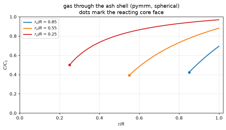
As the core shrinks the shell thickens, the profile steepens, and the
ash resistance grows without bound, which is why ash control gives a
conversion curve that flattens rather than a straight line.
What pymrm adds
Nothing to Eq. 6: it is closed-form, and the page says so. What the numerics add is an answer to the question the three-regime split creates and never resolves.
Textbooks present the three limiting laws and leave the reader to decide which applies. That decision has a quantitative answer: for each \((\omega,\gamma)\), compute the full Eq. 6 and ask how far the nearest single-resistance law is from it. The result is a map with hard boundaries. The map is a grid count, so it is computed on a ladder of grids and the finest is the one quoted.
NG = (90, 180, 360, 720)
MAPS = {}
for ng in NG:
    g = np.logspace(-3, 3, ng)
    MAPS[ng] = (g, *regime_map(g, g))
f5 = {ng: float(np.mean(MAPS[ng][2] < 0.05)) for ng in NG}
f2 = {ng: float(np.mean(MAPS[ng][2] < 0.02)) for ng in NG}
emax = {ng: float(MAPS[ng][2].max()) for ng in NG}
print(f"{'grid':>10}{'within 5 %':>12}{'within 2 %':>12}{'worst error':>13}{'at omega':>10}{'gamma':>8}")
for ng in NG:
    g, best, err = MAPS[ng]
    i, j = np.unravel_index(err.argmax(), err.shape)
    print(f"{ng:6d}^2 {100*f5[ng]:11.2f}%{100*f2[ng]:11.2f}%{100*emax[ng]:12.2f}%{g[j]:10.1f}{g[i]:8.2f}")

FIN = NG[-1]
g_fin, best_fin, err_fin = MAPS[FIN]
claims.value("frac_within_5pct", f5[FIN])
claims.value("frac_within_2pct", f2[FIN])
claims.value("worst_single_law_error", emax[FIN])
claims.bound("map_fraction_change_finest", max(abs(f5[FIN] - f5[NG[-2]]), abs(f2[FIN] - f2[NG[-2]])), max=1e-3,
             basis="chosen", note="last doubling of the grid changes the fractions by less than a tenth of a percentage point")
N5 = claims.count("map_cells_within_5pct", err_fin, 0.05, above=False, min_margin=1e-8,
                  note="no cell lies within a relative 1e-8 of the 5 % threshold, so the count is not decided by round-off")
N2 = claims.count("map_cells_within_2pct", err_fin, 0.02, above=False, min_margin=1e-8,
                  note="no cell lies within a relative 1e-8 of the 2 % threshold, so the count is not decided by round-off")

BAD_LAWS = dict(LAWS, ash=lambda X: 1 - 3 * (1 - X) ** (2 / 3) + (1 - X))
g90 = MAPS[90][0]
_, e_law = regime_map(g90, g90, laws=BAD_LAWS)
_, e_cub = regime_map(g90, g90, cubic="misread")
for lab, e in (("ash law with (1-X) in place of 2(1-X), on the 90 x 90 grid (regime_map(..., laws=...))", e_law),
               ("cubic coefficient read as omega (1 - gamma), on the 90 x 90 grid (regime_map(..., cubic='misread'))", e_cub)):
    brk(lab, "frac_within_5pct", float(np.mean(e < 0.05)))
    brk(lab, "frac_within_2pct", float(np.mean(e < 0.02)))
    if e is e_cub:   # the worst error lies far from the ash corner: only a misread of eq. (6) itself moves it
        brk(lab, "worst_single_law_error", float(e.max()))
brk("ladder stopped at 90 and 180 per decade pair", "map_fraction_change_finest",
    max(abs(f5[180] - f5[90]), abs(f2[180] - f2[90])))
brk("5 % threshold applied as 5e-3 (a factor ten off)", "map_cells_within_5pct", int(np.sum(err_fin < 5e-3)))
brk("2 % threshold applied as 2e-3 (a factor ten off)", "map_cells_within_2pct", int(np.sum(err_fin < 2e-3)))

# The crest: the grid maximum is a kink (film law and reaction law tie), so maximise over gamma directly.
CR3 = crest(1e3)
CR6 = crest(1e6)
claims.value("crest_error_omega1e3", CR3[1], rtol=1e-3)
claims.value("crest_error_omega1e6", CR6[1], rtol=1e-3)
claims.value("crest_gamma_omega1e6", CR6[0], rtol=5e-3)
SH3 = resistance_shares(1e3, CR3[0])
SH6 = resistance_shares(1e6, CR6[0])
claims.bound("crest_reaction_share_omega1e3", SH3[0], max=1e-3, basis="theory",
             note="reaction resistance over the sum of the three at the crest, at the edge of the map; it falls as 1/omega")
print(f"crest at omega = 1e3 (map edge): gamma {CR3[0]:.4f}, error {100*CR3[1]:.3f} %, "
      f"resistance shares reaction/ash/film {100*SH3[0]:.2f}/{100*SH3[1]:.1f}/{100*SH3[2]:.1f} %")
print(f"crest at omega = 1e6: gamma {CR6[0]:.4f}, error {100*CR6[1]:.3f} %, "
      f"resistance shares {100*SH6[0]:.5f}/{100*SH6[1]:.1f}/{100*SH6[2]:.1f} %")
_BAD_REACTION = dict(LAWS, reaction=lambda X: 1 - (1 - X) ** 0.5)
for _om, _name in ((1e3, "crest_error_omega1e3"), (1e6, "crest_error_omega1e6"), (1e6, "crest_gamma_omega1e6")):
    _i = 0 if "gamma" in _name else 1
    brk("gamma scan of 90 points in place of the bounded maximum (crest(..., method='grid', n_scan=90))", _name,
        crest(_om, method="grid", n_scan=90)[_i])
    brk("reaction law with exponent 1/2 in place of 1/3 (crest(..., laws=...))", _name,
        crest(_om, laws=_BAD_REACTION)[_i])
brk("crest taken at omega = 10 in place of the map edge omega = 1e3", "crest_reaction_share_omega1e3",
    resistance_shares(10.0, crest(10.0)[0])[0])

fig, ax = plt.subplots(1, 2, figsize=(12.4, 4.6))
ax[0].pcolormesh(g_fin, g_fin, best_fin, cmap=plt.get_cmap("Set2", 3), shading="auto")
ax[0].set(xscale="log", yscale="log", xlabel=r"$\omega = k_{c1}/k_{d1}$", ylabel=r"$\gamma = 3k_{f1}/k_{d1}$",
          title="which single-resistance law is closest")
for lab, (ox, oy) in (("reaction", (3e-3, 3e2)), ("ash", (3e2, 3e2)), ("film", (3e2, 3e-3))):
    ax[0].text(ox, oy, lab, fontsize=10, fontweight="bold", ha="left", va="center")
cs = ax[1].contourf(g_fin, g_fin, err_fin, levels=[0, 0.01, 0.02, 0.05, 0.10, 0.20, 1.0], cmap="YlOrRd")
ax[1].contour(g_fin, g_fin, err_fin, levels=[0.05], colors="k", linewidths=1.8)
ax[1].set(xscale="log", yscale="log", xlabel=r"$\omega = k_{c1}/k_{d1}$", ylabel=r"$\gamma = 3k_{f1}/k_{d1}$",
          title="how wrong the best single law is\n(black line = 5 %)")
fig.colorbar(cs, ax=ax[1], label=r"max error in $\theta/\theta_B$")
fig.tight_layout(); plt.show()

display(Markdown(rf"""
Over this six-decade square of $(\omega, \gamma)$ on the {FIN} x {FIN} grid, some single-resistance law is within
5 % on {100*f5[FIN]:.1f} % of it and within 2 % on {100*f2[FIN]:.1f} %. The last doubling of the grid changes the
fractions by {claims['map_fraction_change_finest']:.1e} at most (bound 1e-3). The worst error anywhere is
{100*emax[FIN]:.1f} %. The grid maximum is not the worst case: the error crests along a line in $\gamma$ near
{CR6[0]:.2f}, where the film law and the reaction law are equally far from eq. (6), a kink that a grid in $\gamma$
undersamples, so the grid argmax wanders (the table above). Maximising over $\gamma$ directly (`crest`) gives
{100*CR3[1]:.2f} % at $\omega$ = 10$^3$, the edge of the map, and {100*CR6[1]:.2f} % at $\omega$ = 10$^6$, at
$\gamma$ = {CR6[0]:.3f}. The crest rises with $\omega$ and the worst case is the limit $\omega \to \infty$, which
the map only approaches. There the reaction resistance is under
{100*claims.metrics['crest_reaction_share_omega1e3']['max']:.1f} % of the total, so along the crest only the film
({100*SH6[2]:.0f} %) and the ash layer ({100*SH6[1]:.0f} %) matter, and both must be kept.
"""))
grid within 5 % within 2 % worst error at omega gamma
90^2 71.21% 51.56% 20.31% 11.1 0.79
180^2 70.94% 51.42% 20.39% 24.6 0.82
360^2 70.85% 51.35% 20.45% 51.7 0.84
720^2 70.83% 51.30% 20.47% 128.0 0.85
crest at omega = 1e3 (map edge): gamma 0.8545, error 20.486 %, resistance shares reaction/ash/film 0.05/46.1/53.9 %
crest at omega = 1e6: gamma 0.8553, error 20.489 %, resistance shares 0.00005/46.1/53.9 %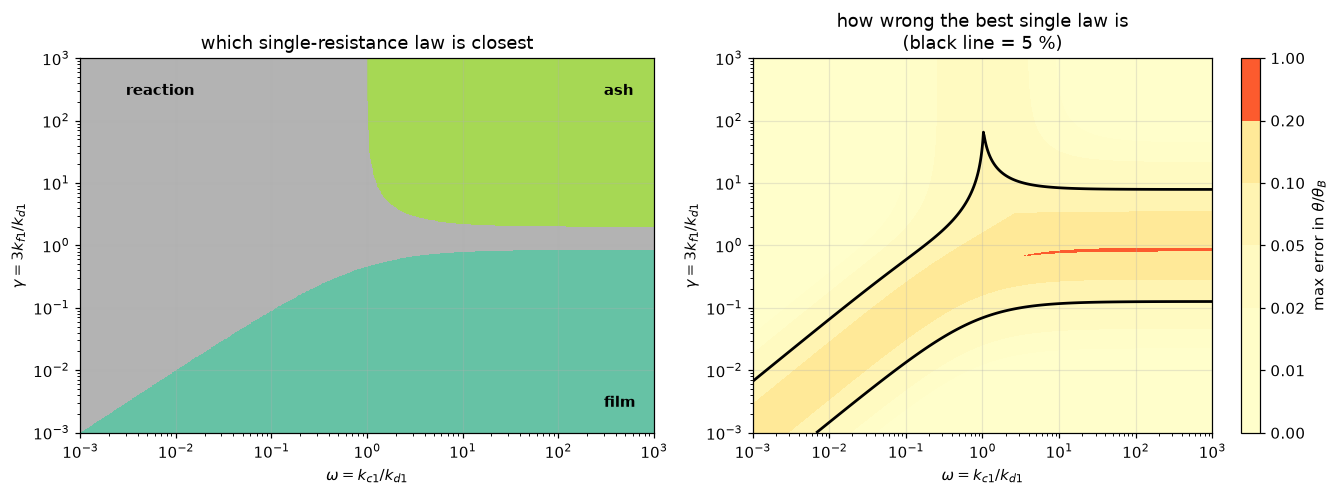
Over this six-decade square of \((\omega, \gamma)\) on the 720 x 720 grid, some single-resistance law is within 5 % on 70.8 % of it and within 2 % on 51.3 %. The last doubling of the grid changes the fractions by 5.0e-04 at most (bound 1e-3). The worst error anywhere is 20.5 %. The grid maximum is not the worst case: the error crests along a line in \(\gamma\) near 0.86, where the film law and the reaction law are equally far from eq. (6), a kink that a grid in \(\gamma\) undersamples, so the grid argmax wanders (the table above). Maximising over \(\gamma\) directly (crest) gives 20.49 % at \(\omega\) = 10\(^3\), the edge of the map, and 20.49 % at \(\omega\) = 10\(^6\), at \(\gamma\) = 0.855. The crest rises with \(\omega\) and the worst case is the limit \(\omega \to \infty\), which the map only approaches. There the reaction resistance is under 0.1 % of the total, so along the crest only the film (54 %) and the ash layer (46 %) matter, and both must be kept.
The break table
Every number above is registered as a claim; each row injects one defect through an argument or a parameter and reports what the claim becomes, and whether the claim’s own check catches it.
print(f"{'injected defect':<92} {'claim':<28} {'clean':>11} {'broken':>11}  caught")
for row, metric, clean, broken, caught in BREAK:
    is_bound = claims.metrics[metric]["kind"] == "bound"
    if is_bound:
        shown, br = f"(here {clean:.3g})", f"{float(broken):.3g}"
        if metric == "shell_finest_over_roundoff":   # round-off of the broken ladder differs per machine
            br = f"(here {float(broken):.2g})"
    else:
        shown, br = f"{float(clean):11.5g}", f"{float(broken):11.5g}"
    print(f"{row[:92]:<92} {metric[:28]:<28} {shown:>11} {br:>11}  {'yes' if caught else 'NO'}")
_caught = {m for _, m, _, _, c in BREAK if c}
_open = sorted(k for k in claims.metrics if k not in _caught)
print(f"\n{len(BREAK)} rows; {len(_caught)} of {len(claims.metrics)} claims are failed by at least one row; "
      f"open: {', '.join(_open) or 'none'}")
print("rows that do not fail their claim: "
      + ("; ".join(f"{r} -> {m}" for r, m, _, _, c in BREAK if not c) or "none"))
injected defect claim clean broken caught
cubic coefficient read as omega (1 - gamma) (eq6(..., cubic='misread')) eq6_endpoint_x1 (here 0) 0.998 yes
film term without the factor 3 (groups(..., film_factor=1)) eq6_vs_integrated_worst (here 6.87e-16) 0.0811 yes
k_d1 = 6 D/D_p instead of 12 D/D_p (groups(..., kd_coef=6)) eq6_vs_integrated_worst (here 6.87e-16) 0.057 yes
limit parameters 1e-5 instead of 1e-9 (ash: omega = 1e5 instead of 1e7) eq6_to_film_limit (here 8.21e-10) 8.21e-06 yes
limit parameters 1e-5 instead of 1e-9 (ash: omega = 1e5 instead of 1e7) eq6_to_ash_limit (here 2.35e-08) 2.35e-06 yes
limit parameters 1e-5 instead of 1e-9 (ash: omega = 1e5 instead of 1e7) eq6_to_reaction_limit (here 3.85e-10) 3.85e-06 yes
ladder 1e-1 and 1e-5: outside the linear range limit_gap_scaling_dev (here 8.72e-06) 0.0792 yes
spherical geometry replaced by cylindrical (Shell(..., nu=1)) shell_solve_worst_rel_err 2.0546e-06 0.59302 yes
reaction condition written with the inward normal (Shell(..., inner_normal='inward')) shell_solve_worst_rel_err 2.0546e-06 14.286 yes
film resistance dropped, bulk value at the surface (Shell(..., film=False)) shell_solve_worst_rel_err 2.0546e-06 17.609 yes
flow read from the first two cells at the core radius (read='cells_at_core') shell_solve_worst_rel_err 2.0546e-06 0.011564 yes
flow read from the first two cells at the core radius (read='cells_at_core') shell_order_finest_min (here 1.9) 0.962 yes
flow read from the first two cells at the core radius (read='cells_at_core') shell_order_finest_max (here 1.97) 0.998 yes
film flow from the last cell value instead of the surface value (flow_outer(read='cell')) shell_conservation_gap (here 3.26e-12) 0.00438 yes
flow read from the first two cells at the core radius (read='cells_at_core') shell_interior_face_gap (here 2.81e-14) 0.0116 yes
ladder 200 to 3200 cells, where the differences approach round-off shell_finest_over_roundoff (here 3.14e+03) (here 4) yes
ash law with (1-X) in place of 2(1-X), on the 90 x 90 grid (regime_map(..., laws=...)) frac_within_5pct 0.70832 0.54099 yes
ash law with (1-X) in place of 2(1-X), on the 90 x 90 grid (regime_map(..., laws=...)) frac_within_2pct 0.51297 0.40988 yes
cubic coefficient read as omega (1 - gamma), on the 90 x 90 grid (regime_map(..., cubic='mis frac_within_5pct 0.70832 0.41272 yes
cubic coefficient read as omega (1 - gamma), on the 90 x 90 grid (regime_map(..., cubic='mis frac_within_2pct 0.51297 0.29889 yes
cubic coefficient read as omega (1 - gamma), on the 90 x 90 grid (regime_map(..., cubic='mis worst_single_law_error 0.20471 0.998 yes
ladder stopped at 90 and 180 per decade pair map_fraction_change_finest (here 0.000502) 0.00272 yes
5 % threshold applied as 5e-3 (a factor ten off) map_cells_within_5pct 3.6719e+05 1.532e+05 yes
2 % threshold applied as 2e-3 (a factor ten off) map_cells_within_2pct 2.6592e+05 94303 yes
gamma scan of 90 points in place of the bounded maximum (crest(..., method='grid', n_scan=90 crest_error_omega1e3 0.20486 0.2026 yes
reaction law with exponent 1/2 in place of 1/3 (crest(..., laws=...)) crest_error_omega1e3 0.20486 0.12622 yes
gamma scan of 90 points in place of the bounded maximum (crest(..., method='grid', n_scan=90 crest_error_omega1e6 0.20489 0.2027 yes
reaction law with exponent 1/2 in place of 1/3 (crest(..., laws=...)) crest_error_omega1e6 0.20489 0.12623 yes
gamma scan of 90 points in place of the bounded maximum (crest(..., method='grid', n_scan=90 crest_gamma_omega1e6 0.85527 0.87866 yes
reaction law with exponent 1/2 in place of 1/3 (crest(..., laws=...)) crest_gamma_omega1e6 0.85527 0.39667 yes
crest taken at omega = 10 in place of the map edge omega = 1e3 crest_reaction_share_omega1e (here 0.000461) 0.0421 yes
31 rows; 22 of 22 claims are failed by at least one row; open: none
rows that do not fail their claim: noneWhat no row can detect. A systematic misreading of both Eq. 5 and Eq. 6 in the same way would move the two routes of check 2 together; the factor 3 and the 12 are caught only because the integration route is built from physical coefficients and not from the printed groups.
What this page does not establish. No experimental comparison, by construction: the source paper’s measurements are of a different model, and inventing agreement would be worse than admitting there is none. The regime map is a statement about Eq. 6, not about any real particle: mapping a given particle onto it requires \(k_{c1}\), which cannot be recovered from the paper as printed. Constant particle size is assumed throughout; a solid that sheds its ash is a different problem with a different exponent. And the quasi-steady assumption behind both Eq. 6 and the shell solve is not tested here. It is excellent for gas-solid systems because the gas holdup in the shell is smaller than the solid inventory by the ratio of the gas to the solid molar density, but that is an argument rather than a measurement.
Reuse
eq6(x, omega, gamma) is the whole model and needs nothing else: two dimensionless groups in, conversion history out. For a particle whose coefficients you know, groups(kc, kf, D, R) converts them, using the paper’s own \(k_{d1} = 12\mathbb{D}_{vs}/D_p\).
Shell is the reusable pymrm piece. A spherical shell with a Robin condition at each face is the geometry of every ash-layer, product-layer or shell-progressive problem, and it extends directly: make \(\mathbb{D}\) a function of radius for a sintering ash layer, or add a source term for a solid that also reacts internally. Read a boundary flux with compute_boundary_values on the boundary dictionary the solve used: that is the flux the solve conserves, and the page measures its conservation. A two-cell difference is the discrete flux through the face at its midpoint, second-order accurate and not exact; it equals the flux through a neighbouring face only while the cell between them has no accumulation and no source (here, the first cell against the core face). With a source term the two differ at first order, and so does the same difference read at any other radius.
The sign trap. Both boundary conditions use the outward normal. At the core face that normal points toward the centre, so the reacting condition reads \(\mathbb{D}\,\partial C/\partial n + k_c C = 0\) with \(d = 0\), structurally identical to the film condition, not opposite to it. Write it with the inward normal and the core will appear to emit gas (the break table keeps the row).
Reading this paper. The scan’s text layer is not usable for equations: it gives \(\theta_B\) as 0B, drops the exponents in Eq. 6’s numerator, and turns Table 1’s velocity range into 0.00 1-0.249. Render at 600 dpi. Table 2 and Table 3 transcribe cleanly if you need the elutriation data.
Related pages. B3.2, B3.3 (other gas-solid conversion models), I1.8, B1.1 (the porous-particle counterpart, where the reaction is distributed rather than at a front).
Cite the source, not this page: Yagi, S. and Kunii, D., Studies on combustion of carbon particles in flames and fluidized beds, 5th Symposium (International) on Combustion, 231-244 (1955).
# Claims: prints every registered number, writes agreement.json for CI, and
# raises when a claim fails its own check or has no break row.
claims.report();   # the semicolon keeps the notebook from echoing the payload
Claims for B3.1:
eq6_endpoint_x1 = (here 0.0e+00) bound bound <= 1e-14 [identity]
eq6_vs_integrated_worst = (here 6.9e-16) bound bound <= 1e-14 [identity]
eq6_to_film_limit = (here 8.2e-10) bound bound <= 1e-09 [theory]
eq6_to_ash_limit = (here 2.3e-08) bound bound <= 3e-08 [theory]
eq6_to_reaction_limit = (here 3.8e-10) bound bound <= 5e-10 [theory]
limit_gap_scaling_dev = (here 8.7e-06) bound bound <= 0.0001 [theory]
shell_solve_worst_rel_err = 2.0546e-06 value rtol 0.05
shell_order_finest_min = (here 1.9e+00) bound bound [1.85, 2.05] [theory]
shell_order_finest_max = (here 2.0e+00) bound bound [1.85, 2.05] [theory]
shell_conservation_gap = (here 3.3e-12) bound bound <= 1e-10 [identity]
shell_interior_face_gap = (here 2.8e-14) bound bound <= 1e-12 [identity]
shell_finest_over_roundoff = (here 3.1e+03) bound bound >= 1000 [theory]
frac_within_5pct = 0.70832 value rtol 0.05
frac_within_2pct = 0.51297 value rtol 0.05
worst_single_law_error = 0.20471 value rtol 0.05
map_fraction_change_finest = (here 5.0e-04) bound bound <= 0.001 [chosen]
map_cells_within_5pct = 367193 exact exact, margin 1.17e-07
map_cells_within_2pct = 265924 exact exact, margin 1.43e-05
crest_error_omega1e3 = 0.20486 value rtol 0.001
crest_error_omega1e6 = 0.20489 value rtol 0.001
crest_gamma_omega1e6 = 0.85527 value rtol 0.005
crest_reaction_share_omega1e3 = (here 4.6e-04) bound bound <= 0.001 [theory]