Thiele modulus and the Weisz–Hicks non-isothermal pellet

sec:B

struct:S3

struct:S10

tier:T0

data:tier6

phase:gas-solid

The effectiveness factor from Thiele’s exact isothermal solution to Weisz and Hicks’ non-isothermal pellet, where η exceeds 100 and three steady states coexist.

Published

July 25, 2026

Modified

November 3, 2026

Thiele modulus and the Weisz–Hicks non-isothermal pellet

Catalog ID: B1.1 + B1.5 · Structures: S3 (1D steady BVP), S10 (constrained/DAE continuation) · Tier: T0

How much of a catalyst pellet actually works? Thiele answered it in 1939 for the isothermal case with a formula still used daily. Weisz and Hicks showed in 1962 that once the pellet is allowed to heat up, the same question has up to three answers at once, and the pellet can run more than a hundred times faster than its own surface conditions suggest.

# Bootstrap: the pymrm this page was checked with, and the gallery files it was
# published with. Works in a checkout, in CI and on a fresh Colab VM.
GALLERY_REF = "gallery-2026.11.10.3"  # replaced by the release tag at publication
PYMRM = ">=3.3.0,<4"  # equals meta.yaml pymrm_min_version, up to the next major
PAGE = "B1.1-thiele-weisz-hicks"  # equals the page directory

import os, sys, urllib.request
from pathlib import Path
_shared = next((p / "shared" for p in (Path.cwd(), *Path.cwd().parents)
                if (p / "shared" / "gallery_bootstrap.py").is_file()), None)
if _shared is None:
    _shared = (Path(os.environ.get("XDG_CACHE_HOME") or Path.home() / ".cache")
               / "pymrm-gallery" / GALLERY_REF)
    _shared.mkdir(parents=True, exist_ok=True)
    urllib.request.urlretrieve(
        "https://raw.githubusercontent.com/computational-chemical-engineering/"
        f"pymrm-gallery/{GALLERY_REF}/shared/gallery_bootstrap.py",
        _shared / "gallery_bootstrap.py")
sys.path.insert(0, str(_shared))
sys.modules.pop("gallery_bootstrap", None)
from gallery_bootstrap import setup
setup(PAGE, PYMRM, GALLERY_REF);  # the semicolon stops the cell echoing the path

import numpy as np
import pandas as pd
import matplotlib.pyplot as plt
from IPython.display import Markdown, display
from scipy.special import iv
from gallery_utils import load_data, load_meta, cite_data, Claims
from model import (NU, Pellet, wh_rate, CentrePinned, trace_branch, trace_branch_own,
                   wh_reference, locate_folds, reference_states)

plt.rcParams.update({"figure.dpi": 110, "axes.grid": True, "grid.alpha": 0.3})
claims = Claims(PAGE.split("-")[0])

Background

A porous catalyst pellet consumes reactant faster than diffusion can resupply its interior, so the inside runs at a lower concentration than the surface. The effectiveness factor \(\eta\) is the ratio of the actual rate to the rate the pellet would achieve if its interior were all at surface conditions.

Thiele (1939) solved the isothermal first-order case exactly. The answer depends on a single dimensionless group, now called the Thiele modulus, comparing reaction rate to diffusion rate. Everything collapses onto one curve: \(\eta\to1\) for small \(\phi\) (kinetics-controlled), \(\eta\to\) (const)\(/\phi\) for large \(\phi\) (diffusion-controlled).

Weisz and Hicks (1962) removed the isothermal assumption. An exothermic reaction heats the pellet interior, the rate constant rises exponentially with temperature, and the two effects fight: depletion lowers the rate, heating raises it. Heating can win outright — \(\eta\) can exceed 1 by orders of magnitude. Worse, over a window of \(\phi\) the steady-state equation has three solutions: a cold, nearly-unused pellet; an ignited one running far above surface temperature; and an unstable state in between.

That is not a numerical artefact. It is the pellet-scale version of the ignition behaviour that makes fixed-bed reactors run away, and it is why the two papers belong on one page.

The published model

Isothermal (Thiele). For a first-order reaction in a pellet of characteristic dimension \(R\),

\[ D_{\mathrm{eff}}\,\nabla^2 c = k\,c , \qquad \left.\frac{\mathrm{d}c}{\mathrm{d}r}\right|_{r=0} = 0 , \qquad c(R) = c_s , \]

with \(\phi = R\sqrt{k/D_{\mathrm{eff}}}\). The exact solutions are

\[ \eta_{\text{slab}} = \frac{\tanh\phi}{\phi}, \qquad \eta_{\text{cyl}} = \frac{2 I_1(\phi)}{\phi\,I_0(\phi)}, \qquad \eta_{\text{sph}} = \frac{3}{\phi^2}\left(\phi\coth\phi - 1\right). \]

Non-isothermal (Weisz–Hicks). Add the energy balance. Because both balances have the same source term, temperature and concentration are linked algebraically by the Prater relation, \(\lambda_{\mathrm{eff}}(T-T_s) = (-\Delta H) D_{\mathrm{eff}}(c_s-c)\), which eliminates \(T\) entirely. With \(y = c/c_s\) and \(u = r/R\) the whole problem reduces to one equation in three dimensionless groups:

\[ \nabla^2 y \;=\; \phi^2\, y \,\exp\!\left[\frac{\gamma\beta(1-y)}{1+\beta(1-y)}\right], \qquad y(1) = 1, \qquad \left.\frac{\mathrm{d}y}{\mathrm{d}u}\right|_{0} = 0 , \]

\[ \beta = \frac{(-\Delta H)\,D_{\mathrm{eff}}\,c_s}{\lambda_{\mathrm{eff}}\,T_s} \quad\text{(Prater number, the maximum relative temperature rise)}, \qquad \gamma = \frac{E}{R_g T_s} \quad\text{(Arrhenius number)} . \]

The effectiveness factor follows from the surface flux, \(\eta = \dfrac{\nu+1}{\phi^{2}}\left.\dfrac{\mathrm{d}y}{\mathrm{d}u}\right|_{u=1}\), with \(\nu = 0,1,2\) for slab, cylinder and sphere.

Symbol	Code	Meaning
\(y\)	`y`	dimensionless concentration \(c/c_s\)
\(\phi\)	`phi`	Thiele modulus
\(\beta\)	`beta`	Prater number
\(\gamma\)	`gamma`	Arrhenius number
\(\nu\)	`nu`	geometry index passed to `construct_div`
\(\eta\)	`eta_from(...)`	effectiveness factor from the surface flux

Parameters and assumptions

Assumptions: steady state; first-order intrinsic kinetics; constant \(D_{\mathrm{eff}}\) and \(\lambda_{\mathrm{eff}}\); no external film resistance (\(y=1\) at the surface); Prater relation exact, which requires the same \(D_{\mathrm{eff}}\) for the reactant in both balances.

The problem is fully dimensionless, so there are no physical parameters to verify — only \(\phi\), \(\beta\), \(\gamma\) and the geometry. Weisz and Hicks tabulated \(\gamma = 20\), which is typical of real catalysis (\(E \approx 100\,\mathrm{kJ\,mol^{-1}}\) at 600 K), and \(\beta\) from 0 to about 0.8.

A note on what serves as “data” here. Neither source paper reports experimental measurements: Thiele (1939) is analytical and Weisz–Hicks (1962) is computational. This page is therefore validated against exact solutions rather than experiment — provenance tier 6 in docs/data-strategy.md. The isothermal comparison is against closed-form expressions; the non-isothermal one is against an independent shooting solution of the same equation. Both are genuine tests of the discretisation, but neither is a test against nature. Experimental effectiveness-factor measurements do exist elsewhere in the literature and would make a worthwhile companion page.

GEOMS = ["slab", "cylinder", "sphere"]
N_ISO = 200                         # cells for the isothermal comparison [-]
GAMMA = 20.0                        # Arrhenius number E/(R_g T_s) [-], Weisz and Hicks
BETAS = [0.0, 0.2, 0.4, 0.6, 0.8]   # Prater numbers of the diagram [-]
BETA_M, N_R = 0.6, 400              # the multiplicity case: Prater number [-], cells [-]

The data

The exact isothermal solutions, tabulated so the validation below is reproducible and checkable by CI.

ref = load_data("isothermal-exact.csv", page=PAGE)
meta = load_meta("isothermal-exact.csv", page=PAGE)
print(cite_data(meta))
print(f"\n{len(ref)} reference values, "
      f"{ref['geometry'].nunique()} geometries, "
      f"phi from {ref['phi'].min():.2f} to {ref['phi'].max():.0f}")
ref.head()

Thiele, E. W. (1939) — Industrial & Engineering Chemistry 31(7) 916-920 — doi:10.1021/ie50355a027 — analytical

180 reference values, 3 geometries, phi from 0.05 to 100

	geometry	phi	eta
0	slab	0.050000	0.999167
1	slab	0.056875	0.998923
2	slab	0.064695	0.998607
3	slab	0.073590	0.998199
4	slab	0.083708	0.997671

PyMRM implementation

The model code is in this page’s model.py, which the first cell put on the path. One class, Pellet, covers every case. The geometry is a single argument — nu=0, 1, 2 in construct_div for slab, cylinder and sphere — and the reaction is passed in, so the isothermal and Weisz–Hicks problems share all the discretisation. The boundary conditions use pymrm’s outward normal: at the centre {"a": 1, "b": 0, "d": 0} is the symmetry condition \(-\mathrm{d}y/\mathrm{d}u = 0\), at the surface {"a": 0, "b": 1, "d": 1} is \(y = 1\). The operators are assembled once; NumJac works on the shape (n_r, 1), so the Jacobian of the pointwise rate is diagonal.

The effectiveness factor is taken from the surface-flux row of the flux operator, not by re-integrating the source term. That is both cheaper and more accurate, because it is the same discrete flux the solver balanced.

For the non-isothermal case, CentrePinned makes \(\psi = \phi^2\) an unknown and adds one equation that pins the centre value, and trace_branch sweeps that centre value with pymrm.continuation. The Results explain why.

Three choices, each checked below:

The S-curve is traced by the library’s continuation. The page’s own warm-start loop, trace_branch_own, traces it a second way, and the two are compared point by point.
The rate is written without clipping at \(y = 0\) and the Newton solves pass no bounds: the Weisz–Hicks rate is smooth and first order through zero, which is what pymrm’s pitfall P9 asks for, and a bound is meant for unknowns the residual cannot accept, not for physical positivity. No solve on the page reaches a negative value.
The folds are located by refining the turning points of the reference curve, and the steady states at the probe modulus are root-found on the reference and solved by Newton on the pymrm pellet. Reading them off the sampled curves instead is computed beside them in the Results.

# Show the model the page runs (model.py next to this notebook).
import inspect, model
print(inspect.getsource(model.Pellet._build_operators))
print(inspect.getsource(model.CentrePinned.__call__))

    def _build_operators(self):
        # outward normal: -r at the centre, +r at the surface (pitfalls P1)
        bc = ({"a": 1.0, "b": 0.0, "d": 0.0},   # u = 0: -dy/du = 0, symmetry
              {"a": 0.0, "b": 1.0, "d": 1.0})   # u = 1: y = 1, surface value
        grad_mat, grad_bc = construct_grad(self.shape, self.r_f, self.r_c, bc)
        div_mat = construct_div(self.shape, self.r_f, nu=self.nu)  # 0 slab, 1 cylinder, 2 sphere
        self.flux_mat, self.flux_bc = -grad_mat, -grad_bc
        self.jac_diff = (div_mat @ self.flux_mat).tocsc()
        self.g_diff = (div_mat @ self.flux_bc).toarray().ravel()
        # the surface-flux row: eta is read from the flux the solver balanced
        self.surf = np.asarray(self.flux_mat[[-1], :].todense()).ravel()
        self.surf_bc = float(self.flux_bc.toarray().ravel()[-1])
        # The rate is pointwise in y, so its Jacobian is diagonal; the
        # tridiagonal coupling is in jac_diff, added analytically.
        self.numjac = NumJac(self.shape)

    def __call__(self, x, y_c):
        """Residual and Jacobian at centre value ``y_c``, for :func:`pymrm.continuation`."""
        p = self.pellet
        y, psi = x[:-1], x[-1]
        g_r, jac_r = p.numjac(self.rate, y.reshape(p.shape))
        g = np.vstack([
            p.jac_diff @ y.reshape((-1, 1)) + p.g_diff.reshape((-1, 1))
            + psi * g_r.reshape((-1, 1)),
            np.array([[y[0] - y_c]]),
        ])
        jac = bmat([[p.jac_diff + psi * jac_r, csc_array(g_r.reshape((-1, 1)))],
                    [self._pin, None]], format="csc")
        return g, jac

Results

Isothermal — against Thiele’s exact solution

phi_grid = np.geomspace(0.05, 100.0, 60)
COL = dict(zip(GEOMS, ["tab:blue", "tab:orange", "tab:green"]))


def eta_numeric(geom, n_r=N_ISO, nu=None, phis=phi_grid):
    """Isothermal eta of the pymrm pellet over a range of Thiele moduli."""
    pellet = Pellet(geom, n_r=n_r, nu=nu)
    return np.array([pellet.solve_linear(f)[1] for f in phis])


def eta_exact_table(geom):
    return ref[ref["geometry"] == geom].sort_values("phi")["eta"].values


def iso_errors(num, mask=None):
    """Worst relative error against the exact table, over geometries."""
    m = np.ones_like(phi_grid, bool) if mask is None else mask
    return max(np.max(np.abs(num[g] - eta_exact_table(g))[m] / eta_exact_table(g)[m])
               for g in GEOMS)


num = {g: eta_numeric(g) for g in GEOMS}

fig, axes = plt.subplots(1, 2, figsize=(11.5, 4.4))
for g in GEOMS:
    ex = ref[ref["geometry"] == g].sort_values("phi")
    axes[0].loglog(ex["phi"], ex["eta"], color=COL[g], lw=2, label=f"{g} (exact)")
    axes[0].loglog(phi_grid[::3], num[g][::3], "o", color=COL[g], ms=6,
                   mfc="white", mew=1.6, label="_nolegend_")
    rel = np.abs(num[g] - ex["eta"].values) / ex["eta"].values
    axes[1].loglog(phi_grid, rel, color=COL[g], lw=2, label=g)

axes[0].set_xlabel(r"Thiele modulus, $\phi$ [-]")
axes[0].set_ylabel(r"effectiveness factor, $\eta$ [-]")
axes[0].set_title("Lines: exact.  Markers: pymrm")
axes[0].legend(frameon=False)
axes[1].set_xlabel(r"Thiele modulus, $\phi$ [-]")
axes[1].set_ylabel("relative error [-]")
axes[1].set_title(r"pymrm vs exact, $n_r = 200$")
axes[1].legend(frameon=False)
fig.tight_layout(); plt.show()

LO = phi_grid <= 30.0
iso_err = iso_errors(num)
iso_err_lo = iso_errors(num, LO)
print(f"worst relative error, phi <= 30   : {iso_err_lo:.3e}")
print(f"worst relative error, all phi     : {iso_err:.3e}")
print("\nThe error is concentrated at large phi, where the reactant is consumed")
print("in a surface layer of thickness ~1/phi that a uniform grid cannot resolve.")

ETA_EX_100 = (3 / 100.0**2) * (100.0 / np.tanh(100.0) - 1)


def err_phi100(n_r, nu=None):
    """Relative eta error of the sphere at phi = 100 on n_r cells."""
    return abs(Pellet("sphere", n_r=n_r, nu=nu).solve_linear(100.0)[1] - ETA_EX_100) / ETA_EX_100


print("\nSame point (sphere, phi = 100) under uniform refinement:")
ERR_100 = {}
prev = None
for n in (200, 400, 800, 1600):
    ERR_100[n] = e = err_phi100(n)
    rate_txt = f"  ({prev/e:.1f}x)" if prev else ""
    print(f"   n_r = {n:5d}:  relative error {e:.3e}{rate_txt}")
    prev = e
iso_err_fine = ERR_100[1600]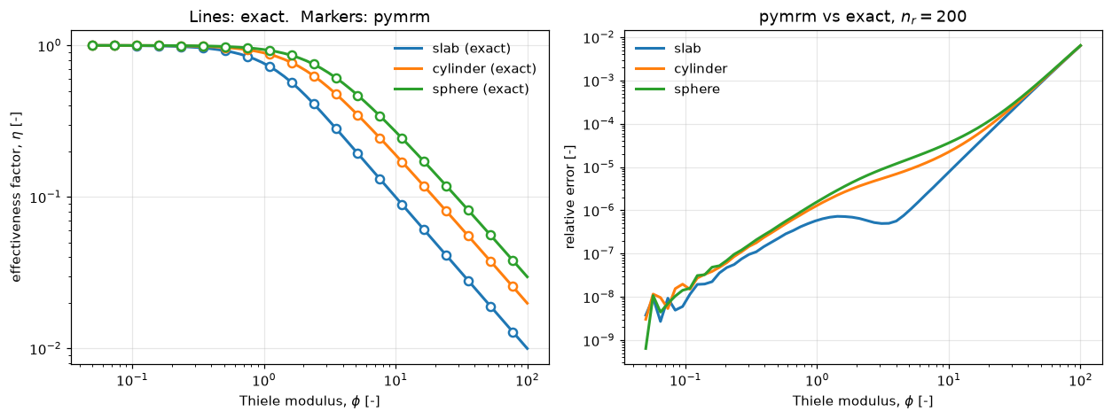

worst relative error, phi <= 30   : 2.248e-04
worst relative error, all phi     : 6.464e-03

The error is concentrated at large phi, where the reactant is consumed
in a surface layer of thickness ~1/phi that a uniform grid cannot resolve.

Same point (sphere, phi = 100) under uniform refinement:
   n_r =   200:  relative error 6.464e-03
   n_r =   400:  relative error 9.369e-04  (6.9x)
   n_r =   800:  relative error 1.324e-04  (7.1x)
   n_r =  1600:  relative error 1.933e-05  (6.8x)

The Aris collapse

Thiele’s three curves are really one. Using the generalised modulus \(\Lambda = (V_p/A_p)\sqrt{k/D_{\mathrm{eff}}}\) — Aris’s characteristic length, the volume-to-surface ratio — all geometries fall close to \(\tanh\Lambda/\Lambda\). The collapse is exact in both asymptotes and loosest in the transition region around \(\Lambda \approx 1\), where the three geometries still differ by about 15%. That is the accuracy of the “shape doesn’t matter” shortcut, and it is worth knowing the number rather than assuming it is negligible.

VA = {"slab": 1.0, "cylinder": 0.5, "sphere": 1.0 / 3.0}   # (V/A)/R

fig, ax = plt.subplots(figsize=(7.5, 4.4))
lam_ref = np.geomspace(0.02, 40, 200)
ax.loglog(lam_ref, np.tanh(lam_ref) / lam_ref, "k--", lw=1.6,
          label=r"$\tanh\Lambda/\Lambda$ (slab)")
for g in GEOMS:
    ax.loglog(phi_grid * VA[g], num[g], color=COL[g], lw=2, label=g)
ax.set_xlabel(r"generalised modulus, $\Lambda = (V_p/A_p)\sqrt{k/D_{\rm eff}}$ [-]")
ax.set_ylabel(r"$\eta$ [-]")
ax.set_title("All geometries collapse onto one curve")
ax.legend(frameon=False)
fig.tight_layout(); plt.show()


def aris_spread(va, curves=None):
    """Largest relative spread between the geometries at equal Lambda, 0.3 to 3."""
    curves = num if curves is None else curves
    spread = []
    for L in np.geomspace(0.3, 3.0, 25):
        vals = [np.interp(L, phi_grid * va[g], curves[g]) for g in GEOMS]
        spread.append((max(vals) - min(vals)) / np.mean(vals))
    return max(spread)


ARIS_SPREAD = aris_spread(VA)
print(f"max spread between geometries at equal Lambda (0.3-3): {ARIS_SPREAD:.1%}")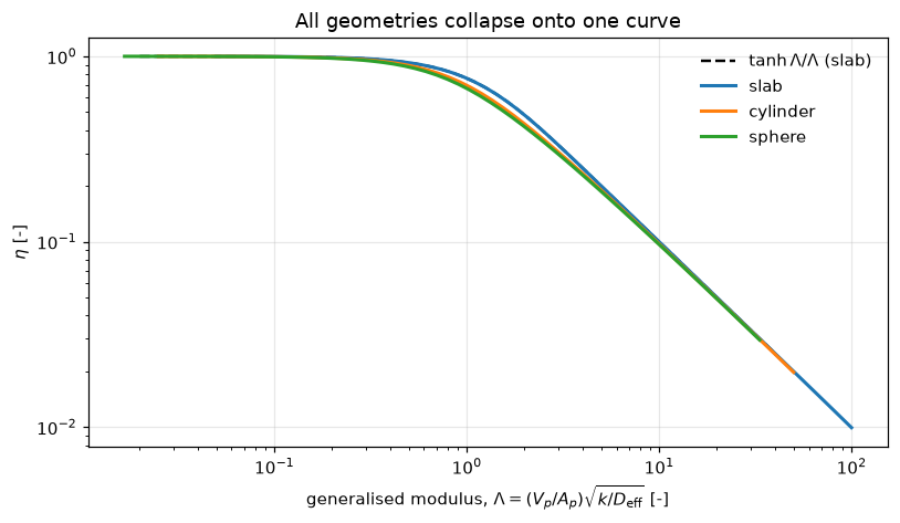

max spread between geometries at equal Lambda (0.3-3): 15.4%

Non-isothermal — the Weisz–Hicks diagram

Now switch on the heat. Each curve is one Prater number \(\beta\) at \(\gamma = 20\). \(\beta\) is the maximum relative temperature rise the pellet can generate, so \(\beta = 0.6\) means the centre can run 60% above surface temperature in absolute terms — enough to swamp the depletion effect entirely.

The curves come from the independent shooting reference wh_reference: with \(s = \phi u\) the equation no longer contains \(\phi\), so integrating outward from a chosen centre value until \(y = 1\) gives \(\phi\), and the curve is a single-valued function of the centre value.

Y_DIAGRAM = np.geomspace(1e-6, 0.9995, 170)


def wh_curve(beta, gamma=GAMMA, y_scan=Y_DIAGRAM):
    """Reference (phi, eta) along increasing centre values."""
    return np.array([q for v in y_scan for q in [wh_reference(beta, gamma, v)] if q])


def fold_depth(curve):
    """How far phi falls back while the centre value decreases, relative to its
    running maximum: 0 for a curve that is a function of phi."""
    phi = curve[::-1, 0]
    run_max = np.maximum.accumulate(phi)
    return float(np.max((run_max - phi) / run_max))


cmap = plt.cm.viridis(np.linspace(0.05, 0.85, len(BETAS)))
fig, ax = plt.subplots(figsize=(8, 5))
wh_curves = {}
for beta, c in zip(BETAS, cmap):
    wh_curves[beta] = pts = wh_curve(beta)
    ax.loglog(pts[:, 0], pts[:, 1], color=c, lw=2, label=rf"$\beta$ = {beta}")

ax.axhline(1.0, color="k", lw=0.8, ls=":")
ax.set_xlabel(r"Thiele modulus, $\phi$ [-]")
ax.set_ylabel(r"effectiveness factor, $\eta$ [-]")
ax.set_title(rf"Weisz–Hicks diagram, $\gamma$ = {GAMMA:.0f} (sphere)")
ax.legend(frameon=False, title="Prater number")
fig.tight_layout(); plt.show()

FOLD_DEPTH = {beta: fold_depth(wh_curves[beta]) for beta in BETAS}
ETA_MAX = {beta: float(wh_curves[beta][:, 1].max()) for beta in BETAS}
for beta in BETAS:
    print(f"beta={beta:.1f}:  eta_max = {ETA_MAX[beta]:8.2f}   "
          f"multivalued in phi: {FOLD_DEPTH[beta] > 1e-3}")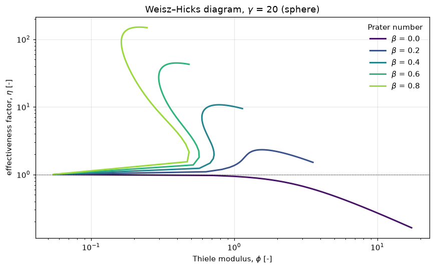

beta=0.0:  eta_max =     1.00   multivalued in phi: False
beta=0.2:  eta_max =     2.32   multivalued in phi: False
beta=0.4:  eta_max =    10.73   multivalued in phi: True
beta=0.6:  eta_max =    44.55   multivalued in phi: True
beta=0.8:  eta_max =   151.22   multivalued in phi: True

Two things to notice. The \(\beta = 0\) curve is Thiele’s isothermal result. Every other curve rises above \(\eta = 1\) — the pellet outperforms its own surface conditions, because its interior is hotter; at \(\beta = 0.8\) the effectiveness factor reaches 151. And from \(\beta = 0.4\) upward the curve folds back on itself: it is no longer a function of \(\phi\).

Three steady states at one Thiele modulus

Where the curve folds, a single \(\phi\) admits three solutions. Continuation in \(\phi\) cannot pass a fold: the branch turns there, and the corrector either fails or jumps to another branch. Newton at a fixed \(\phi\) finds the middle, unstable state only from a guess already close to it, and a pseudo-time march never settles on it.

The fix costs four lines: make \(\phi^2\) an unknown, and add one algebraic equation pinning the centre concentration. Along the centre value the curve is single valued, so continuation in that parameter traces the whole S-curve, unstable branch included. This is structure S10 — a constrained/DAE system — assembled with scipy.sparse.bmat around the same pymrm operators (CentrePinned in model.py), and swept with pymrm.continuation, which predicts each point from the previous two (a secant) and checks that the corrector did not jump branches.

pellet = Pellet("sphere", n_r=N_R)
rate_m = wh_rate(BETA_M, GAMMA)
problem = CentrePinned(pellet, rate_m)

# Sweep the centre concentration from ~1 (uniform pellet) down to 1e-7 (fully
# ignited); the ignited branch lives at very small centre values. The two
# segments meet at 0.1; the second starts one point later, so that no value is
# visited twice.
YC = np.concatenate([1.0 - np.geomspace(1e-6, 0.9, 120),
                     np.geomspace(0.1, 1e-7, 200)[1:]])

branch, branch_x, cont = trace_branch(problem, YC)
print(f"pymrm.continuation: {cont.message}")
print(f"traced {len(branch)} points, y_centre from {branch[:,2].max():.3f}"
      f" down to {branch[:,2].min():.1e}")
y_min_ignited = float(branch_x[-1][:-1].min())

pymrm.continuation: Reached every parameter value
traced 319 points, y_centre from 1.000 down to 1.0e-07

The reference locates the folds: the scan brackets each turning point of \(\phi\) along the centre value and a bounded scalar minimisation refines it, so the result does not depend on the scan spacing. The probe modulus \(\phi^\ast\) is the geometric mean of the two folds. At \(\phi^\ast\) the reference states are root-found along the centre value, and the pymrm states are solved by Newton at fixed \(\phi^\ast\), each starting from the nearest point of the traced branch, the middle one included.

Y_SCAN = np.geomspace(1e-8, 0.9995, 120)
folds = locate_folds(BETA_M, GAMMA, Y_SCAN)
(phi_lo, yc_lo, _), (phi_hi, yc_hi, _) = folds
phi_star = float(np.sqrt(phi_lo * phi_hi))
roots = reference_states(BETA_M, GAMMA, phi_star, Y_SCAN)


def pymrm_states(pel, rate, phi, branch, branch_x, centres, **newton_kwargs):
    """Newton at fixed phi from the branch point nearest to each centre value."""
    out = []
    for y_c in centres:
        k = int(np.argmin(np.abs(branch[:, 2] - y_c)))
        y, eta, res = pel.solve_nonlinear(phi, rate, y_init=branch_x[k][:-1],
                                          **newton_kwargs)
        out.append((eta, float(y[0]), bool(res.success), int(res.nit)))
    return out


states = pymrm_states(pellet, rate_m, phi_star, branch, branch_x, [r[1] for r in roots])
eta_ignited = roots[-1][0]
probe_dev = max(abs(s[0] - r[0]) / r[0] for s, r in zip(states, roots))

# the 900-point reference curve of the figure, and the sampled reading compared
# below: folds read off its samples, states interpolated linearly
ref_m = np.array([(q[0], q[1], v) for v in np.geomspace(1e-8, 0.9995, 900)
                  for q in [wh_reference(BETA_M, GAMMA, v)] if q])


def sampled_folds(curve):
    """Turning points of phi at the sample points, the two most prominent."""
    phi = curve[:, 0]
    turn = np.where(np.diff(np.sign(np.diff(phi))) != 0)[0] + 1
    prom = [min(abs(phi[i] - phi[:i].min()), abs(phi[i] - phi[i:].max())) for i in turn]
    turn = [t for _, t in sorted(zip(prom, turn), reverse=True)[:2]]
    return sorted(phi[turn])


def crossings(curve, phi_target):
    """Linearly interpolated eta wherever the curve crosses phi_target."""
    out = []
    for i in np.where(np.diff(np.sign(curve[:, 0] - phi_target)))[0]:
        f = (phi_target - curve[i, 0]) / (curve[i + 1, 0] - curve[i, 0])
        out.append(curve[i, 1] + f * (curve[i + 1, 1] - curve[i, 1]))
    return sorted(out)


smp_lo, smp_hi = sampled_folds(ref_m)
smp_star = float(np.sqrt(smp_lo * smp_hi))
smp_ref, smp_pym = crossings(ref_m, smp_star), crossings(branch, smp_star)
interp_dev = max(abs(a - b) / b for a, b in zip(smp_ref, smp_pym))

fig, ax = plt.subplots(figsize=(8, 5))
ax.loglog(ref_m[:, 0], ref_m[:, 1], "-", color="0.7", lw=4,
          label="shooting reference")
ax.loglog(branch[:, 0], branch[:, 1], color="tab:red", lw=2,
          label="pymrm continuation")
ax.axvspan(phi_lo, phi_hi, color="tab:orange", alpha=0.13, lw=0,
           label="three steady states")
ax.axvline(phi_star, color="k", lw=0.9, ls="--")
for e, _ in roots:
    ax.plot(phi_star, e, "o", color="k", ms=8, mfc="white", mew=2, zorder=6)
ax.set_xlabel(r"Thiele modulus, $\phi$ [-]")
ax.set_ylabel(r"effectiveness factor, $\eta$ [-]")
ax.set_title(rf"$\beta$ = {BETA_M}, $\gamma$ = {GAMMA:.0f}: the fold")
ax.legend(frameon=False, loc="upper left")
fig.tight_layout(); plt.show()

print(f"multiplicity window: {phi_lo:.4f} < phi < {phi_hi:.4f}")
print(f"\nat phi = {phi_star:.4f}, steady states found by each method:")
print(f"   {'reference':>12} {'pymrm':>12}   pymrm Newton at fixed phi")
for (e_r, _), (e_p, _, ok, nit) in zip(roots, states):
    print(f"   {e_r:12.3f} {e_p:12.3f}   converged {ok} in {nit} iterations")
print(f"largest relative difference: {probe_dev:.1e}")
print(f"\nratio of the ignited to the extinguished branch: "
      f"{eta_ignited/roots[0][0]:.0f}x")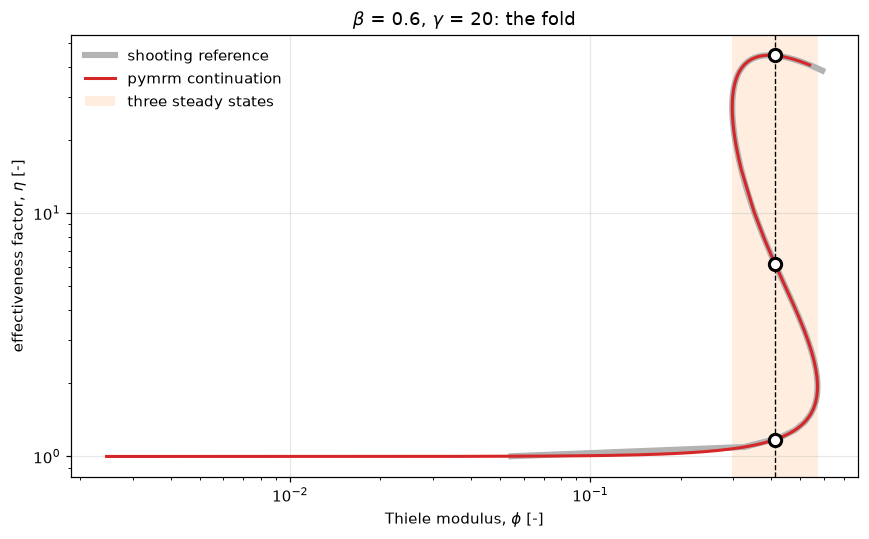

multiplicity window: 0.2973 < phi < 0.5719

at phi = 0.4123, steady states found by each method:
      reference        pymrm   pymrm Newton at fixed phi
          1.173        1.173   converged True in 4 iterations
          6.205        6.205   converged True in 4 iterations
         44.450       44.450   converged True in 4 iterations
largest relative difference: 1.4e-05

ratio of the ignited to the extinguished branch: 38x

Why the folds are refined and the states root-found. The cell below reads the folds off the 900 sample points of the reference curve and interpolates both curves linearly at \(\phi^\ast\). The upper fold sits where the samples are sparse, so its sampled value is off by about 1e-4, and the interpolated states differ from each other by up to 3e-3 (6.207 on the reference against 6.225 on pymrm, on the middle branch), which looks like a discretisation error of that size. It is interpolation: at equal centre value, and at fixed \(\phi^\ast\) above, pymrm and the reference agree to about 1e-5.

display(pd.DataFrame({
    "sampled, interpolated": [smp_lo, smp_hi, smp_star, *smp_ref, *smp_pym],
    "refined, root-found, Newton": [phi_lo, phi_hi, phi_star,
                                          *[r[0] for r in roots], *[s[0] for s in states]],
}, index=["lower fold", "upper fold", "probe phi*", "reference: extinguished",
          "reference: unstable", "reference: ignited", "pymrm: extinguished",
          "pymrm: unstable", "pymrm: ignited"]).round(6))

	sampled, interpolated	refined, root-found, Newton
lower fold	0.297321	0.297321
upper fold	0.571789	0.571859
probe phi*	0.412317	0.412342
reference: extinguished	1.176668	1.173073
reference: unstable	6.206816	6.205482
reference: ignited	44.450209	44.449920
pymrm: extinguished	1.173360	1.173074
pymrm: unstable	6.225159	6.205397
pymrm: ignited	44.450334	44.450208

A second route: the page’s own warm-start loop

trace_branch_own traces the branch with a plain loop: each centre value starts Newton from the previous solution, and a solve that fails is skipped while the march goes on. pymrm.continuation adds a secant predictor, halves the step when a solve fails, refuses a corrector that jumps to another branch, and stops with a message instead of skipping. Here every point converges with both, and the two branches agree to the Newton tolerance.

own, own_failed = trace_branch_own(problem, YC)
own_gap_psi = float(np.max(np.abs(own[:, 0] ** 2 - branch[:, 0] ** 2)))


def branch_folds(br):
    """Turning points of phi at the traced points."""
    phi = br[:, 0]
    turn = np.where(np.diff(np.sign(np.diff(phi))) != 0)[0] + 1
    return sorted(phi[turn])


lib_lo, lib_hi = branch_folds(branch)
own_lo, own_hi = branch_folds(own)
own_fold_gap = max(abs(own_lo - lib_lo) / lib_lo, abs(own_hi - lib_hi) / lib_hi)
print(f"own loop: {len(own)} points converged, {own_failed} failed")
print(f"largest |phi^2 (own) - phi^2 (library)| over the branch: below 1e-9 "
      f"(here {own_gap_psi:.1e})")
print(f"folds at the traced points, library: {lib_lo:.6f}  {lib_hi:.6f}")
print(f"folds at the traced points, own    : {own_lo:.6f}  {own_hi:.6f}")
print(f"folds of the reference, refined    : {phi_lo:.6f}  {phi_hi:.6f}")

own loop: 319 points converged, 0 failed
largest |phi^2 (own) - phi^2 (library)| over the branch: below 1e-9 (here 4.0e-12)
folds at the traced points, library: 0.297321  0.571732
folds at the traced points, own    : 0.297321  0.571732
folds of the reference, refined    : 0.297321  0.571859

The folds read at the traced points are the extremes of a sampled curve, like the sampled reading above, so the upper one is again low by a similar amount: the sweep’s points are sparse there too. The refined reference value is the one the page reports.

Validation

Four checks, then the register of every number the page states and the defect-injection table.

# 1. Isothermal, against the exact closed form (all three geometries).
print(f"1. worst relative eta error vs exact       : {iso_err:.3e}")

# 2. Grid convergence at phi = 5: second order for the scheme.
ETA5 = {"slab": np.tanh(5.0) / 5.0,
        "cylinder": 2 * iv(1, 5.0) / (5.0 * iv(0, 5.0)),
        "sphere": (3 / 25.0) * (5.0 / np.tanh(5.0) - 1)}
EPS = np.finfo(float).eps


def grid_order(geom, ns=(50, 100, 200, 400), nu=None, phi=5.0):
    """Observed order between the two finest grids, and the finest error over its
    round-off estimate n^2 eps (the condition number of the operator times eps)."""
    exact = ETA5[geom] if phi == 5.0 else {"slab": np.tanh(phi) / phi}[geom]
    e = [abs(Pellet(geom, n_r=n, nu=nu).solve_linear(phi)[1] - exact) / exact
         for n in ns]
    return float(np.log2(e[-2] / e[-1])), e[-1] / (ns[-1] ** 2 * EPS)


ORDERS, ROUNDOFF = {}, {}
for g in GEOMS:
    ORDERS[g], ROUNDOFF[g] = grid_order(g)
order_mean = float(np.mean([ORDERS[g] for g in GEOMS]))
print("2. observed order of convergence at phi=5  : "
      + ", ".join(f"{g} {ORDERS[g]:.2f}" for g in GEOMS) + f"   (mean {order_mean:.2f})")
ORDER_SLAB_PHI1 = grid_order("slab", phi=1.0)[0]
print(f"   slab at phi = 1                         : {ORDER_SLAB_PHI1:.2f}")
print(f"   finest error over its round-off estimate: at least 1000 "
      f"(here {min(ROUNDOFF.values()):.1e})")

# 3. Non-isothermal: compare at EQUAL centre concentration, which is the
#    parameter both methods share, so no interpolation is involved.


def vs_reference(br, beta=BETA_M):
    dev_eta, dev_phi = [], []
    for phi_b, eta_b, y_c in br[::7]:
        q = wh_reference(beta, GAMMA, y_c)
        if q:
            dev_phi.append(abs(phi_b - q[0]) / q[0])
            dev_eta.append(abs(eta_b - q[1]) / q[1])
    return float(np.median(dev_eta)), float(np.median(dev_phi)), len(dev_eta)


med_eta, med_phi, n_cmp = vs_reference(branch)
print(f"3. vs shooting at equal y_centre, median |d.eta|/eta : {med_eta:.3e}")
print(f"                                 median |d.phi|/phi : "
      f"{med_phi:.3e}   ({n_cmp} points)")

# 4. Prater relation: the ignited branch should approach the bound beta.
dT_max = BETA_M * (1.0 - y_min_ignited)
print(f"4. relative temperature rise on the ignited branch   : {dT_max:.4f}"
      f"   (bound is beta = {BETA_M})")

1. worst relative eta error vs exact       : 6.464e-03
2. observed order of convergence at phi=5  : slab 2.96, cylinder 2.06, sphere 2.03   (mean 2.35)
   slab at phi = 1                         : 2.01
   finest error over its round-off estimate: at least 1000 (here 3.6e+03)
3. vs shooting at equal y_centre, median |d.eta|/eta : 1.007e-05
                                 median |d.phi|/phi : 7.623e-06   (46 points)
4. relative temperature rise on the ignited branch   : 0.6000   (bound is beta = 0.6)

All three geometries are second order. The slab’s 2.96 at \(\phi = 5\) is pre-asymptotic: there its \(h^2\) error coefficient happens to be small, so the \(h^3\) term dominates on every grid used here (an independent solve of the same stencil in 34-digit arithmetic shows the observed order falling towards 2 as the grid is refined further). The order depends on \(\phi\): at \(\phi = 1\) the slab gives the second order printed above. The mean of the three geometries, 2.35, mixes the two orders; it is registered as a claim with the range that mixture implies.

Claims: what each number is, and how it is checked

Every number the page stands behind is registered once, in the cell below (docs/claims-design.md in the gallery repository):

a value is a result whose size is set by physics or by the discretisation. CI holds it to a relative tolerance of the committed baseline, 5 % unless the cell says otherwise;
a bound is a quantity whose size is not physics: a solver-tolerance gap, a convergence order, a physical limit. It is checked against its stated limits on every run, on every machine, and states its basis;
an exact result is a count or a label, with its distance to the threshold that decided it where there is one.

Fold locations carry a relative tolerance of 1e-5 and the reference states at the probe one of 1e-3: they are refined extremes and roots of a smooth function integrated to a relative accuracy of 1e-10, identical under three BLAS kernels, and the tolerances have to be that tight for the sampled-fold row and the Arrhenius row to fail them (the extinguished state moves by only 0.5 % when the Arrhenius number rises by 2 %).

# --- isothermal --------------------------------------------------------------
claims.value("isothermal_max_rel_error_phi_le_30", iso_err_lo)
claims.value("isothermal_max_rel_error_all_phi", iso_err)
claims.value("isothermal_err_phi100_n400", ERR_100[400])
claims.value("isothermal_err_phi100_n800", ERR_100[800])
claims.value("isothermal_err_phi100_n1600", iso_err_fine)
claims.value("aris_max_spread", ARIS_SPREAD)
for g, lo_, hi_ in (("slab", 2.7, 3.1), ("cylinder", 1.9, 2.2), ("sphere", 1.9, 2.2)):
    claims.bound(f"convergence_order_{g}", ORDERS[g], min=lo_, max=hi_,
                 basis="theory" if g != "slab" else "chosen",
                 note=None if g != "slab" else
                 "pre-asymptotic at phi = 5 (small h^2 coefficient, h^3 dominates on "
                 "these grids); the scheme is second order")
claims.bound("convergence_order_slab_phi1", ORDER_SLAB_PHI1, min=1.9, max=2.2,
             basis="theory")
claims.bound("convergence_order", order_mean, min=2.2, max=2.5, basis="chosen",
             note="mean of the slab (about 3) and cylinder and sphere (2)")
claims.bound("convergence_finest_over_roundoff", min(ROUNDOFF.values()), min=1e3,
             basis="theory", note="claims-design section 3: the order is not fitted to noise")
# --- the Weisz-Hicks diagram --------------------------------------------------
claims.bound("eta_max_beta0", ETA_MAX[0.0], min=0.99, max=1.0, basis="theory",
             note="isothermal first order: eta < 1, approached as phi -> 0")
for beta in BETAS[1:]:
    claims.value(f"eta_max_beta{beta:.1f}".replace(".", ""), ETA_MAX[beta])
claims.count("n_multivalued_curves", [FOLD_DEPTH[b] for b in BETAS], threshold=1e-3,
             min_margin=0.5, note="curves whose phi falls back by more than 0.1 %")
# --- the fold and the three steady states -------------------------------------
claims.value("phi_fold_lower", phi_lo, rtol=1e-5)
claims.value("phi_fold_upper", phi_hi, rtol=1e-5)
claims.value("phi_probe", phi_star, rtol=1e-5)
claims.exact("n_steady_states_at_probe", len(roots),
             margin=min(phi_star / phi_lo - 1, 1 - phi_star / phi_hi), min_margin=0.05)
claims.exact("n_pymrm_states_converged", sum(s[2] for s in states))
for (e_r, _), (e_p, *_), name in zip(roots, states, ("extinguished", "unstable", "ignited")):
    if name != "ignited":
        claims.value(f"eta_{name}", e_r, rtol=1e-3)
    claims.value(f"eta_{name}_pymrm", e_p)
claims.value("eta_ignited", eta_ignited, rtol=1e-3)
claims.value("ignited_over_extinguished", eta_ignited / roots[0][0])
claims.value("probe_pymrm_vs_reference_max_rel", probe_dev)
claims.value("interpolated_states_max_rel_gap", interp_dev)
claims.value("eta_unstable_interpolated_ref", smp_ref[1], rtol=1e-3)
claims.value("eta_unstable_interpolated_pymrm", smp_pym[1], rtol=1e-3)
claims.value("fold_upper_sampled_rel_error", abs(smp_hi - phi_hi) / phi_hi)
# --- continuation: library and the page's own loop ----------------------------
claims.exact("branch_points", len(branch))
claims.value("branch_fold_lower", lib_lo, rtol=1e-6)
claims.value("branch_fold_upper", lib_hi, rtol=1e-6)
claims.bound("own_vs_library_psi_gap", own_gap_psi, max=1e-9, basis="tolerance",
             note="both converge each point to a Newton step below 1e-11")
claims.bound("own_vs_library_fold_gap", own_fold_gap, max=1e-8, basis="tolerance",
             note="the folds at the traced points, relative")
claims.exact("own_loop_failed_points", own_failed)
# --- validation against the shooting reference ---------------------------------
claims.value("nonisothermal_median_dev", med_eta)
claims.value("nonisothermal_median_dev_phi", med_phi)
claims.exact("nonisothermal_points_compared", n_cmp)
claims.bound("prater_rise_gap", BETA_M - dT_max, min=0.0, max=1e-5, basis="chosen",
             note="beta - rise = beta * y_min; the sweep ends at y_centre = 1e-7")

# --- numbers written in the Markdown above ------------------------------------
claims.says("15%", "aris_max_spread")                    # "differ by about 15%"
claims.says("151", "eta_max_beta08")                     # "reaches 151"
claims.says("above 100", "eta_max_beta08")               # description: "eta exceeds 100"
claims.says("2.35", "convergence_order")                 # "the mean ..., 2.35"
claims.says("2.96", "convergence_order_slab")           # "the slab's 2.96"
claims.says("6.225", "eta_unstable_interpolated_pymrm")  # "6.207 ... against 6.225"
claims.says("6.207", "eta_unstable_interpolated_ref")    # "6.207 ... against 6.225"
claims.says("2.2e-4", "isothermal_max_rel_error_phi_le_30")   # What pymrm adds
claims.says("1e-4", "fold_upper_sampled_rel_error")      # "off by about 10^-4"
claims.says("1e-5", "probe_pymrm_vs_reference_max_rel")  # "agree to about 10^-5"
claims.says("1e-5", "nonisothermal_median_dev")          # "agree to about 10^-5"
claims.says("3e-3", "interpolated_states_max_rel_gap")   # "up to 3e-3"
print(f"{len(claims.metrics)} claims registered")

45 claims registered

The defect-injection table

Each row breaks one thing on purpose, re-runs the computation behind one claim with the defect in place, and hands the result to claims.breaks, which records whether the claim’s own check (its tolerance or its bound) catches it. A row that moves its claim by less than the claim’s tolerance is kept, marked as not caught, when what it shows is itself a finding. Every claim must be failed by at least one row, and the last cell of the page raises otherwise.

BREAK = []


def brk(name, metric, value, note=""):
    """One injected defect: ``value`` is what claim ``metric`` becomes with it."""
    caught = claims.breaks(name, metric, value)
    BREAK.append(dict(defect=name, metric=metric, clean=claims[metric], broken=value,
                      caught=caught, note=note))


# --- isothermal: geometry and grid ------------------------------------------
num_bad = dict(num, cylinder=eta_numeric("cylinder", nu=2))
brk("cylinder assembled with nu = 2", "isothermal_max_rel_error_phi_le_30",
    iso_errors(num_bad, LO))
brk("cylinder assembled with nu = 2", "isothermal_max_rel_error_all_phi", iso_errors(num_bad))
num_coarse = {g: eta_numeric(g, n_r=N_ISO // 2) for g in GEOMS}
brk("n_r halved to 100", "isothermal_max_rel_error_phi_le_30", iso_errors(num_coarse, LO))
brk("n_r halved to 100", "isothermal_max_rel_error_all_phi", iso_errors(num_coarse))
for n in (400, 800, 1600):
    brk(f"phi = 100 on n_r = {n // 2} instead of {n}", f"isothermal_err_phi100_n{n}",
        err_phi100(n // 2))
brk("sphere assembled with nu = 1 at phi = 100", "isothermal_err_phi100_n1600",
    err_phi100(1600, nu=1))
brk("cylinder V/A taken as R/3 (the sphere's)", "aris_max_spread",
    aris_spread(dict(VA, cylinder=1.0 / 3.0)))
brk("cylinder curve from nu = 2", "aris_max_spread", aris_spread(VA, num_bad))

# --- convergence orders ---------------------------------------------------------
_wrong = {"slab": 1, "cylinder": 2, "sphere": 1}
_bad_orders = {g: grid_order(g, nu=_wrong[g])[0] for g in GEOMS}
for g in GEOMS:
    brk(f"{g} assembled with nu = {_wrong[g]}", f"convergence_order_{g}", _bad_orders[g],
        "converges to the wrong geometry: the error stops falling")
brk("slab assembled with nu = 1, at phi = 1", "convergence_order_slab_phi1",
    grid_order("slab", nu=1, phi=1.0)[0])
brk("every geometry assembled with the wrong nu", "convergence_order",
    float(np.mean(list(_bad_orders.values()))))
brk("orders fitted on n_r = 3200, 6400", "convergence_finest_over_roundoff",
    min(grid_order(g, ns=(3200, 6400))[1] for g in GEOMS),
    "the slab's finest error is at round-off there")

# --- the Weisz-Hicks diagram ----------------------------------------------------
brk("Prater number 0.1 instead of 0", "eta_max_beta0", float(wh_curve(0.1)[:, 1].max()))
for beta in BETAS[1:]:
    brk("Arrhenius number 5 % low", f"eta_max_beta{beta:.1f}".replace(".", ""),
        float(wh_curve(beta, 0.95 * GAMMA)[:, 1].max()))
_depth_bad = {**FOLD_DEPTH, 0.4: fold_depth(wh_curve(0.4, gamma=12.0))}
brk("Arrhenius number 12 for the beta = 0.4 curve", "n_multivalued_curves",
    int(sum(d > 1e-3 for d in _depth_bad.values())), "gamma*beta = 4.8: unique")

# --- the folds and the steady states ------------------------------------------------
_f_bad = locate_folds(BETA_M * 1.02, GAMMA, Y_SCAN)
brk("Prater number 2 % high", "phi_fold_lower", _f_bad[0][0])
brk("Prater number 2 % high", "phi_fold_upper", _f_bad[1][0])
brk("Prater number 2 % high", "phi_probe", np.sqrt(_f_bad[0][0] * _f_bad[1][0]))
brk("fold read off the 900 samples, not refined", "phi_fold_lower", smp_lo,
    "the lower fold sits where the samples are dense")
brk("fold read off the 900 samples, not refined", "phi_fold_upper", smp_hi)
brk("probe at phi = 0.25, below the lower fold", "n_steady_states_at_probe",
    len(reference_states(BETA_M, GAMMA, 0.25, Y_SCAN)))
_roots_bad = reference_states(BETA_M, GAMMA * 1.02, phi_star, Y_SCAN)
for (e_b, _), name in zip(_roots_bad, ("extinguished", "unstable", "ignited")):
    brk("Arrhenius number 2 % high in the reference", f"eta_{name}", e_b)
brk("Arrhenius number 2 % high in the reference", "ignited_over_extinguished",
    _roots_bad[-1][0] / _roots_bad[0][0])
brk("Arrhenius number 2 % high in the reference", "probe_pymrm_vs_reference_max_rel",
    max(abs(s[0] - r[0]) / r[0] for s, r in zip(states, _roots_bad)))
_pel_bad = Pellet("sphere", n_r=N_R, nu=1)
_states_bad = pymrm_states(_pel_bad, rate_m, phi_star, branch, branch_x,
                           [r[1] for r in roots])
for (e_b, *_), name in zip(_states_bad, ("extinguished", "unstable", "ignited")):
    brk("pymrm pellet assembled with nu = 1", f"eta_{name}_pymrm", e_b)
brk("Newton at fixed phi with maxfev = 2", "n_pymrm_states_converged",
    sum(s[2] for s in pymrm_states(pellet, rate_m, phi_star, branch, branch_x,
                                   [r[1] for r in roots], maxfev=2)))
_pel_25 = Pellet("sphere", n_r=25)
_br_25, _x_25, _ = trace_branch(CentrePinned(_pel_25, rate_m), YC)
_states_25 = pymrm_states(_pel_25, rate_m, phi_star, _br_25, _x_25, [r[1] for r in roots])
brk("pymrm pellet on n_r = 25", "probe_pymrm_vs_reference_max_rel",
    max(abs(s[0] - r[0]) / r[0] for s, r in zip(_states_25, roots)))
_ll_ref = np.exp(crossings(np.log(ref_m[:, :2]), np.log(smp_star)))
_ll_pym = np.exp(crossings(np.log(branch[:, :2]), np.log(smp_star)))
brk("interpolation in log-log coordinates", "interpolated_states_max_rel_gap",
    max(abs(a - b) / b for a, b in zip(_ll_ref, _ll_pym)))
brk("reference interpolated on every tenth sample", "eta_unstable_interpolated_ref",
    min(crossings(ref_m[::10], smp_star), key=lambda e: abs(e - smp_ref[1])),
    "the nearest crossing: so coarse a sample also loses one of the three")
brk("interpolation in log-log coordinates", "eta_unstable_interpolated_pymrm", _ll_pym[1])
brk("upper fold from a 300-point sample", "fold_upper_sampled_rel_error",
    abs(sampled_folds(ref_m[::3])[1] - phi_hi) / phi_hi)

# --- continuation ----------------------------------------------------------------
_br_short, _x_short, _ = trace_branch(problem, YC[YC >= 1e-3])
brk("sweep stopped at y_centre = 1e-3", "branch_points", len(_br_short))
brk("sweep stopped at y_centre = 1e-3", "nonisothermal_points_compared",
    vs_reference(_br_short)[2])
brk("sweep stopped at y_centre = 1e-3", "prater_rise_gap",
    BETA_M * float(_x_short[-1][:-1].min()))
_problem_b = CentrePinned(pellet, wh_rate(BETA_M + 0.01, GAMMA))
_br_b, _, _ = trace_branch(_problem_b, YC)
_dev_b = vs_reference(_br_b)
brk("Prater number 0.61 in the pymrm pellet only", "nonisothermal_median_dev", _dev_b[0])
brk("Prater number 0.61 in the pymrm pellet only", "nonisothermal_median_dev_phi", _dev_b[1])
_bf_b = branch_folds(_br_b)
brk("Prater number 0.61 in the pymrm pellet only", "branch_fold_lower", _bf_b[0])
brk("Prater number 0.61 in the pymrm pellet only", "branch_fold_upper", _bf_b[1])
_own_loose, _ = trace_branch_own(problem, YC, tol=1e-4)
brk("own loop with Newton tol = 1e-4", "own_vs_library_psi_gap",
    float(np.max(np.abs(_own_loose[:, 0] ** 2 - branch[:, 0] ** 2))))
_ol = branch_folds(_own_loose)
brk("own loop with Newton tol = 1e-4", "own_vs_library_fold_gap",
    max(abs(_ol[0] - lib_lo) / lib_lo, abs(_ol[1] - lib_hi) / lib_hi),
    "not caught: tol 1e-4 moves phi^2 by about 1e-8 (row above), too little to "
    "shift which traced point is the extreme")
_ol2 = branch_folds(trace_branch_own(problem, YC[::2])[0])
brk("own loop on every second centre value", "own_vs_library_fold_gap",
    max(abs(_ol2[0] - lib_lo) / lib_lo, abs(_ol2[1] - lib_hi) / lib_hi),
    "the folds at traced points depend on which points are traced")
brk("own loop with maxfev = 2", "own_loop_failed_points",
    trace_branch_own(problem, YC, maxfev=2)[1])

BT = pd.DataFrame(BREAK)


def _shown(metric, v):
    # a bound's digits are this run's and differ between machines: shown as such
    if claims.metrics[metric]["kind"] == "bound":
        return f"(here {float(v):.1e})"
    return f"{v:.4g}" if isinstance(v, float) else str(v)


_table = BT.assign(clean=[_shown(m, v) for m, v in zip(BT.metric, BT.clean)],
                   broken=[_shown(m, v) for m, v in zip(BT.metric, BT.broken)])
with pd.option_context("display.max_colwidth", 70, "display.width", 250,
                       "display.max_rows", 200):
    display(_table[["defect", "metric", "clean", "broken", "caught", "note"]])
_caught = set(BT[BT.caught].metric)
_open = sorted(k for k in claims.metrics if k not in _caught)
print(f"{len(BT)} rows; {int(BT.caught.sum())} fail the claim they target, "
      f"{len(BT) - int(BT.caught.sum())} do not (each says why in its note).")
print(f"{len(_caught)} of {len(claims.metrics)} claims are failed by at least one row.")
print("claims with no failing row:", ", ".join(_open) or "none")

	defect	metric	clean	broken	caught	note
0	cylinder assembled with nu = 2	isothermal_max_rel_error_phi_le_30	0.0002248	0.3332	True
1	cylinder assembled with nu = 2	isothermal_max_rel_error_all_phi	0.006464	0.3332	True
2	n_r halved to 100	isothermal_max_rel_error_phi_le_30	0.0002248	0.001397	True
3	n_r halved to 100	isothermal_max_rel_error_all_phi	0.006464	0.03926	True
4	phi = 100 on n_r = 200 instead of 400	isothermal_err_phi100_n400	0.0009369	0.006464	True
5	phi = 100 on n_r = 400 instead of 800	isothermal_err_phi100_n800	0.0001324	0.0009369	True
6	phi = 100 on n_r = 800 instead of 1600	isothermal_err_phi100_n1600	1.933e-05	0.0001324	True
7	sphere assembled with nu = 1 at phi = 100	isothermal_err_phi100_n1600	1.933e-05	0.005021	True
8	cylinder V/A taken as R/3 (the sphere's)	aris_max_spread	0.1539	0.4473	True
9	cylinder curve from nu = 2	aris_max_spread	0.1539	0.3731	True
10	slab assembled with nu = 1	convergence_order_slab	(here 3.0e+00)	(here 8.1e-05)	True	converges to the wrong geometry: the error stops falling
11	cylinder assembled with nu = 2	convergence_order_cylinder	(here 2.1e+00)	(here 1.4e-04)	True	converges to the wrong geometry: the error stops falling
12	sphere assembled with nu = 1	convergence_order_sphere	(here 2.0e+00)	(here -9.2e-05)	True	converges to the wrong geometry: the error stops falling
13	slab assembled with nu = 1, at phi = 1	convergence_order_slab_phi1	(here 2.0e+00)	(here 2.0e-06)	True
14	every geometry assembled with the wrong nu	convergence_order	(here 2.3e+00)	(here 4.4e-05)	True
15	orders fitted on n_r = 3200, 6400	convergence_finest_over_roundoff	(here 3.6e+03)	(here 3.6e-03)	True	the slab's finest error is at round-off there
16	Prater number 0.1 instead of 0	eta_max_beta0	(here 1.0e+00)	(here 1.2e+00)	True
17	Arrhenius number 5 % low	eta_max_beta02	2.323	2.143	True
18	Arrhenius number 5 % low	eta_max_beta04	10.73	8.883	True
19	Arrhenius number 5 % low	eta_max_beta06	44.55	33.68	True
20	Arrhenius number 5 % low	eta_max_beta08	151.2	106.4	True
21	Arrhenius number 12 for the beta = 0.4 curve	n_multivalued_curves	3	2	True	gamma*beta = 4.8: unique
22	Prater number 2 % high	phi_fold_lower	0.2973	0.286	True
23	Prater number 2 % high	phi_fold_upper	0.5719	0.5655	True
24	Prater number 2 % high	phi_probe	0.4123	0.4022	True
25	fold read off the 900 samples, not refined	phi_fold_lower	0.2973	0.2973	False	the lower fold sits where the samples are dense
26	fold read off the 900 samples, not refined	phi_fold_upper	0.5719	0.5718	True
27	probe at phi = 0.25, below the lower fold	n_steady_states_at_probe	3	1	True
28	Arrhenius number 2 % high in the reference	eta_extinguished	1.173	1.179	True
29	Arrhenius number 2 % high in the reference	eta_unstable	6.205	5.893	True
30	Arrhenius number 2 % high in the reference	eta_ignited	44.45	49.31	True
31	Arrhenius number 2 % high in the reference	ignited_over_extinguished	37.89	41.84	True
32	Arrhenius number 2 % high in the reference	probe_pymrm_vs_reference_max_rel	1.372e-05	0.09864	True
33	pymrm pellet assembled with nu = 1	eta_extinguished_pymrm	1.173	2.275	True
34	pymrm pellet assembled with nu = 1	eta_unstable_pymrm	6.205	5.442	True
35	pymrm pellet assembled with nu = 1	eta_ignited_pymrm	44.45	60.66	True
36	Newton at fixed phi with maxfev = 2	n_pymrm_states_converged	3	0	True
37	pymrm pellet on n_r = 25	probe_pymrm_vs_reference_max_rel	1.372e-05	0.003512	True
38	interpolation in log-log coordinates	interpolated_states_max_rel_gap	0.002947	0.003514	True
39	reference interpolated on every tenth sample	eta_unstable_interpolated_ref	6.207	6.224	True	the nearest crossing: so coarse a sample also loses one of the three
40	interpolation in log-log coordinates	eta_unstable_interpolated_pymrm	6.225	6.209	True
41	upper fold from a 300-point sample	fold_upper_sampled_rel_error	0.0001212	0.003165	True
42	sweep stopped at y_centre = 1e-3	branch_points	319	186	True
43	sweep stopped at y_centre = 1e-3	nonisothermal_points_compared	46	27	True
44	sweep stopped at y_centre = 1e-3	prater_rise_gap	(here 6.0e-08)	(here 6.1e-04)	True
45	Prater number 0.61 in the pymrm pellet only	nonisothermal_median_dev	1.007e-05	0.05855	True
46	Prater number 0.61 in the pymrm pellet only	nonisothermal_median_dev_phi	7.623e-06	0.0336	True
47	Prater number 0.61 in the pymrm pellet only	branch_fold_lower	0.2973	0.2879	True
48	Prater number 0.61 in the pymrm pellet only	branch_fold_upper	0.5717	0.5663	True
49	own loop with Newton tol = 1e-4	own_vs_library_psi_gap	(here 4.0e-12)	(here 2.4e-08)	True
50	own loop with Newton tol = 1e-4	own_vs_library_fold_gap	(here 2.1e-12)	(here 3.3e-12)	False	not caught: tol 1e-4 moves phi^2 by about 1e-8 (row above), too li...
51	own loop on every second centre value	own_vs_library_fold_gap	(here 2.1e-12)	(here 9.4e-04)	True	the folds at traced points depend on which points are traced
52	own loop with maxfev = 2	own_loop_failed_points	0	319	True

53 rows; 51 fail the claim they target, 2 do not (each says why in its note).
45 of 45 claims are failed by at least one row.
claims with no failing row: none

What the checks can and cannot do

The isothermal claims test the operators against an exact solution, so every assembly defect that matters (wrong nu, a coarse grid) moves them. They cannot see an error shared by the solver and the exact table, and there is none to share: the table is evaluated from the closed forms.
The non-isothermal claims compare pymrm with a shooting integration of the same equation. A defect in the model that both share (the wrong rate expression, a wrong Prater relation) would pass them; the Arrhenius and Prater rows show that the claims do move when only one side changes.
prater_rise_gap is close to an identity: once the Prater relation is substituted, the temperature rise is \(\beta(1 - y)\), so the check only says that the sweep reached the ignited branch. The row that stops the sweep early is the defect it catches.
The comparison of the library continuation with the page’s own loop is held at the Newton tolerance; it cannot tell which of the two is right, only that they agree. The reference comparison does that.

What pymrm adds

Nothing, for the isothermal case — and that is the point. Thiele’s formula is exact; the value of reproducing it is that it pins the discretisation to 2.2e-4 for \(\phi \le 30\) and confirms second-order convergence. A page that agrees with an exact solution has earned the right to be believed where no exact solution exists.

For the non-isothermal case, the whole solution branch. Weisz and Hicks could report points; the fold between them had to be inferred. Making \(\phi^2\) an unknown and pinning the centre concentration turns the multivalued curve into a single-valued one, and pymrm.continuation traces it in one sweep, unstable branch included, using the same operators as the isothermal solve. Continuation in \(\phi\) cannot get past the folds, and a pseudo-time march never settles on the unstable branch; Newton at fixed \(\phi\) reaches it from a guess close to it, here one taken off the traced branch, as the table above does.

And geometry is a parameter, not a rewrite. nu=0,1,2 covers slab, cylinder and sphere, and nu also accepts a callable for an arbitrary area profile — which is how non-standard pellet shapes are handled without leaving the 1D formulation.

Reuse

Change	Where
Different geometry	`Pellet(geom=...)`, or pass a callable `nu` to `construct_div` for an arbitrary area profile
Non-first-order kinetics	replace `wh_rate`; keep the rate smooth and first order through zero (pymrm pitfall P9); `NumJac` picks up the new derivative automatically
External film resistance	change the surface boundary condition from `{"a":0,"b":1,"d":1}` to a Robin condition
Multiple reactants	give the field shape `(n_r, n_c)`; `NumJac` couples the last (field) axis in full by default
Another multiplicity problem	pin a quantity along which the branch is single-valued, make the parameter an unknown (`CentrePinned`), and sweep with `pymrm.continuation`
Couple to a reactor	this is the inner problem of `D1.4`; export `eta` or the surface flux

Related pages: B1.2 Aris generalised modulus · B1.4 Weisz–Prater criterion · D1.4 fixed bed with resolved pellets · J4.7 immobilised enzyme particle (same equation, Michaelis–Menten kinetics) · A4.9 Duncan–Toor (shares S3).

References

Thiele, E. W. (1939). Relation between catalytic activity and size of particle. Industrial & Engineering Chemistry 31(7), 916–920. doi:10.1021/ie50355a027

Weisz, P. B. and Hicks, J. S. (1962). The behaviour of porous catalyst particles in view of internal mass and heat diffusion effects. Chemical Engineering Science 17(4), 265–275. doi:10.1016/0009-2509(62)85005-2

Aris, R. (1957). On shape factors for irregular particles. Chemical Engineering Science 6(6), 262–268.

Prater, C. D. (1958). The temperature produced by heat of reaction in the interior of porous particles. Chemical Engineering Science 8(3–4), 284–286.

# Claims: prints every registered number, writes agreement.json for CI, and
# raises when a claim fails its own check or has no break row.
claims.report();   # the semicolon keeps the notebook from echoing the payload

Claims for B1.1:
  isothermal_max_rel_error_phi_le_30 = 0.00022483       value  rtol 0.05
  isothermal_max_rel_error_all_phi   = 0.006464         value  rtol 0.05
  isothermal_err_phi100_n400         = 0.00093686       value  rtol 0.05
  isothermal_err_phi100_n800         = 0.00013241       value  rtol 0.05
  isothermal_err_phi100_n1600        = 1.9331e-05       value  rtol 0.05
  aris_max_spread                    = 0.15394          value  rtol 0.05
  convergence_order_slab             = (here 3.0e+00)   bound  bound [2.7, 3.1] [chosen]
  convergence_order_cylinder         = (here 2.1e+00)   bound  bound [1.9, 2.2] [theory]
  convergence_order_sphere           = (here 2.0e+00)   bound  bound [1.9, 2.2] [theory]
  convergence_order_slab_phi1        = (here 2.0e+00)   bound  bound [1.9, 2.2] [theory]
  convergence_order                  = (here 2.3e+00)   bound  bound [2.2, 2.5] [chosen]
  convergence_finest_over_roundoff   = (here 3.6e+03)   bound  bound >= 1000 [theory]
  eta_max_beta0                      = (here 1.0e+00)   bound  bound [0.99, 1] [theory]
  eta_max_beta02                     = 2.3234           value  rtol 0.05
  eta_max_beta04                     = 10.733           value  rtol 0.05
  eta_max_beta06                     = 44.555           value  rtol 0.05
  eta_max_beta08                     = 151.22           value  rtol 0.05
  n_multivalued_curves               = 3                exact  exact, margin 1
  phi_fold_lower                     = 0.29732          value  rtol 1e-05
  phi_fold_upper                     = 0.57186          value  rtol 1e-05
  phi_probe                          = 0.41234          value  rtol 1e-05
  n_steady_states_at_probe           = 3                exact  exact, margin 0.279
  n_pymrm_states_converged           = 3                exact  exact
  eta_extinguished                   = 1.1731           value  rtol 0.001
  eta_extinguished_pymrm             = 1.1731           value  rtol 0.05
  eta_unstable                       = 6.2055           value  rtol 0.001
  eta_unstable_pymrm                 = 6.2054           value  rtol 0.05
  eta_ignited_pymrm                  = 44.45            value  rtol 0.05
  eta_ignited                        = 44.45            value  rtol 0.001
  ignited_over_extinguished          = 37.892           value  rtol 0.05
  probe_pymrm_vs_reference_max_rel   = 1.3718e-05       value  rtol 0.05
  interpolated_states_max_rel_gap    = 0.0029466        value  rtol 0.05
  eta_unstable_interpolated_ref      = 6.2068           value  rtol 0.001
  eta_unstable_interpolated_pymrm    = 6.2252           value  rtol 0.001
  fold_upper_sampled_rel_error       = 0.00012125       value  rtol 0.05
  branch_points                      = 319              exact  exact
  branch_fold_lower                  = 0.29732          value  rtol 1e-06
  branch_fold_upper                  = 0.57173          value  rtol 1e-06
  own_vs_library_psi_gap             = (here 4.0e-12)   bound  bound <= 1e-09 [tolerance]
  own_vs_library_fold_gap            = (here 2.1e-12)   bound  bound <= 1e-08 [tolerance]
  own_loop_failed_points             = 0                exact  exact
  nonisothermal_median_dev           = 1.0072e-05       value  rtol 0.05
  nonisothermal_median_dev_phi       = 7.6232e-06       value  rtol 0.05
  nonisothermal_points_compared      = 46               exact  exact
  prater_rise_gap                    = (here 6.0e-08)   bound  bound [0, 1e-05] [chosen]